biomass burning and urban air pollution over the central ... · atmos. chem. phys. discuss., 9,...

ACPD9, 2699–2734, 2009

Biomass burningpollution over Central

Mexico

J. D. Crounse et al.

Title Page

Abstract Introduction

Conclusions References

Tables Figures

J I

J I

Back Close

Full Screen / Esc

Printer-friendly Version

Interactive Discussion

Atmos. Chem. Phys. Discuss., 9, 2699–2734, 2009www.atmos-chem-phys-discuss.net/9/2699/2009/© Author(s) 2009. This work is distributed underthe Creative Commons Attribution 3.0 License.

AtmosphericChemistry

and PhysicsDiscussions

This discussion paper is/has been under review for the journal Atmospheric Chemistryand Physics (ACP). Please refer to the corresponding final paper in ACP if available.

Biomass burning and urban air pollutionover the Central Mexican PlateauJ. D. Crounse1, P. F. DeCarlo2,*, D. R. Blake3, L. K. Emmons4, T. L. Campos4,E. C. Apel4, A. D. Clarke5, A. J. Weinheimer4, D. C. McCabe7,**, R. J. Yokelson6,J. L. Jimenez2, and P. O. Wennberg7,8

1Division of Chemistry and Chemical Engineering, California Institute of Technology,Pasadena, CA 91125, USA2University of Colorado, Boulder, CO, USA3Department of Chemistry, University of California at Irvine, Irvine, CA, USA4National Center for Atmospheric Research, Boulder, CO, USA5Department of Oceanography, University of Hawaii, USA6Department of Chemistry, University of Montana, Missoula, MT, USA7Division of Geology and Planetary Sciences, California Institute of Technology, Pasadena,CA, USA8Division of Environmental Science and Engineering, California Institute of Technology,Pasadena, CA, USA

2699

http://www.atmos-chem-phys-discuss.net

http://www.atmos-chem-phys-discuss.net/9/2699/2009/acpd-9-2699-2009-print.pdf

http://www.atmos-chem-phys-discuss.net/9/2699/2009/acpd-9-2699-2009-discussion.html

http://creativecommons.org/licenses/by/3.0/

ACPD9, 2699–2734, 2009


Mexico


Title Page



Tables Figures

J I

J I

Back Close

Full Screen / Esc



* now at: Laboratory of Atmospheric Chemistry, Paul Scherrer Institute, Switzerland** now at: AAAS Science and Technology Policy Fellow, United States Environmental Protec-tion Agency, Washington, DC, USA

Received: 18 November 2008 – Accepted: 25 November 2008 – Published: 28 January 2009

Correspondence to: J. D. Crounse ([email protected])

Published by Copernicus Publications on behalf of the European Geosciences Union.

2700





ACPD9, 2699–2734, 2009


Mexico


Title Page



Tables Figures

J I

J I

Back Close

Full Screen / Esc



Abstract

Observations during the 2006 dry season of highly elevated concentrations of cyanidesin the atmosphere above Mexico City (MC) and the surrounding plains, demonstratethat biomass burning (BB) significantly impacted air quality in the region. We find thatduring the period of our measurements, fires contribute more than half of the organic5

aerosol mass and submicron aerosol scattering, and one third of the enhancementin benzene, reactive nitrogen, and carbon monoxide in the outflow from the plateau.The combination of biomass burning and anthropogenic emissions will affect ozonechemistry in the MC outflow.

1 Introduction10

The 20 Million (2005) inhabitants of Mexico City experience some of the worst air qual-ity in the world. The high population density coupled with the topography of the city(2200 m, surrounded on three sides by mountains) leads to the daily buildup of pollu-tants in the region (Molina and Molina, 2002). Despite growing population and greatlyincreased automobile use, air quality has improved measurably in the last decade as15

the federal and city governments implemented a series of air quality regulations broadlysimilar to those that have been effective in, for example, Los Angeles (Lloyd, 1992).Nevertheless, ozone and particulate matter (PM) in the city often exceed internationalstandards (WHO, 2008) and the city is consistently enveloped in a pall by the largeamount of aerosol present.20

The pollution from the city has impacts beyond the basin. Aerosols and ozone pro-duce important forcing on regional climate through their interaction with both thermalinfrared and visible radiation (Solomon et al., 2007). Indeed, the effluents from megac-ities, such as Mexico City, are now seen as globally important sources of pollution.

In the last decade, there have been several intensive studies of the air quality in the25

Mexico City basin. A major study undertaken in the Mexico City Metropolitan Area

2701





ACPD9, 2699–2734, 2009


Mexico


Title Page



Tables Figures

J I

J I

Back Close

Full Screen / Esc



in spring of 2003 (MCMA-2003) included significant international cooperation (Molinaet al., 2007). In the spring of 2006, a consortium of atmospheric scientists expandedsignificantly on this study, obtaining a large suite of measurements in and around Mex-ico City in an effort to understand both the controlling chemistry in the basin and theimpacts of the outflow pollution on the broader region. Named, Megacity Initiative:5

Local and Global Research Observations (MILAGRO), this campaign involved mea-surements at several ground sites along the most common outflow trajectory, and fromseveral aircraft. The National Science Foundation (NSF) C-130 (operated by the Na-tional Center for Atmospheric Research (NCAR)), and the US Forest Service TwinOtter, along with several other aircraft operated from Veracruz, Mexico. Here, we focus10

on observations made from the C-130 aircraft on seven flights above the Central Mex-ican Plateau. Details about the broader MILAGRO study are reviewed by Fast et al.(2007).

Most efforts to engineer improvements in Mexico City air quality have logically fo-cused on reducing emissions from the transportation and power generation sectors15

(McKinley et al., 2005) and on new liquefied petroleum gas (LPG) regulations. How-ever, as in Los Angeles, as the emissions from transportation and industrial sectorsdecline, continued improvement in air quality will require addressing additional sources.

Biomass burning can be a significant contributor to poor air quality in many regions ofthe world, including southern California (Muhle et al., 2007). Several previous studies20

have suggested that fires in and around the Mexico City basin can impact air quality(Molina et al., 2007; Bravo et al., 2002; Salcedo et al., 2006). During the springtime(March–May), many fires occur in the pine forests on the mountains surrounding thecity, both inside and outside the basin. Typically, the biomass burning season intensifiesin late March, reaching a maximum in May (Fast et al., 2007; Bravo et al., 2002).25

The heat from these fires is observable from space by the infrared channels of themoderate resolution imaging spectroradiometer (MODIS) instruments operated fromNASA’s Aqua and Terra platforms (Giglio et al., 2003). Figure 1, for example, showstwo visible images from MODIS taken on 5 March (panel a) and 10 March (panel b)

2702





ACPD9, 2699–2734, 2009


Mexico


Title Page



Tables Figures

J I

J I

Back Close

Full Screen / Esc



2006. The locations of the detected thermal anomalies are shown as red boxes. Theaerosol haze from the fires can be seen covering large areas of land around and aboveMC, particularly on 5 March. MODIS imagery suggests that the total biomass burningaround MC in March 2006 was greater than climatological amounts, and closer to whatis normally observed during the month of April.5

Using tracers of pollution from biomass burning and urban emissions, we show thatfires significantly impacted air quality above and downwind of Mexico City in March2006. We use aircraft measurements of hydrogen cyanide (HCN) to estimate the con-tribution of biomass burning to the regional air quality. HCN is produced in the pyrolysisof amino acids (Ratcliff et al., 1974) and has been widely used as an atmospheric tracer10

of biomass burning emissions (e.g., Li et al., 2003). We use simultaneous observationsof acetylene (C2H2) to characterize the contribution of urban emissions. We show thata simple two end-member mixing model (biomass burning and urban emissions) de-veloped from these tracers can explain most of the observed variability in several pol-lutants including carbon monoxide, benzene, organic aerosol, reactive nitrogen oxides15

(NOy), and the amount of submicron aerosol particles.

2 Observations

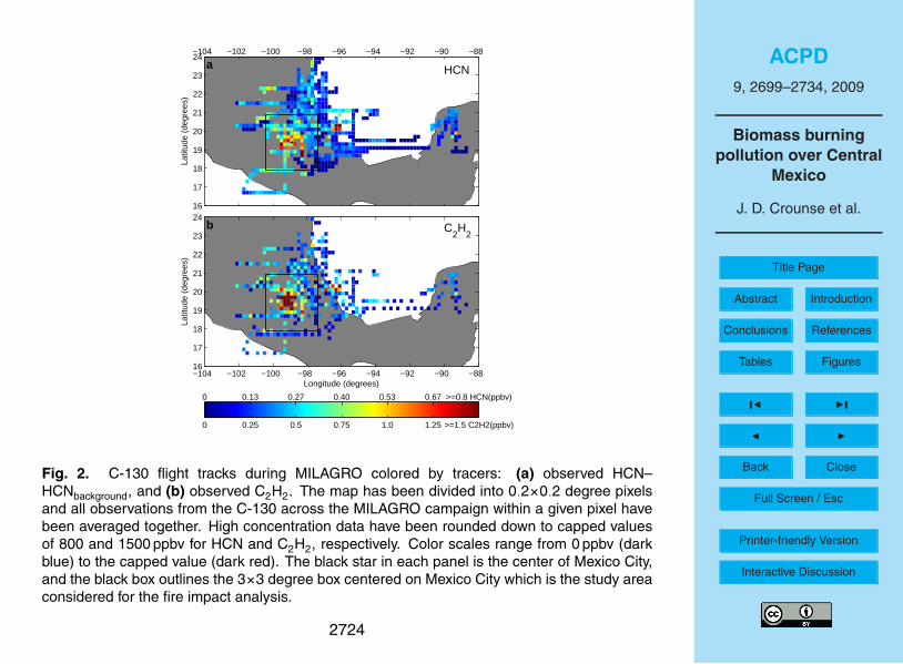
The NSF C-130 flew through the Mexico City region on eleven flights in March 2006(Fig. 2). Of these flights, three had fewer than ten samples of C2H2 within our studyarea (3×3 degree box centered on MC, and termed Central Mexican Plateau) and one20

flight did not have HCN observations. These flights are excluded from the calculationof the overall fire impact (4, 12, 26, and 28 March). In Fig. 2a, the aircraft flight tracksare colored by the average amount of HCN measured in the air. Acetonitrile (CH3CN)mixing ratios, which also have been used extensively as a biomass burning tracer, werehighly correlated (r2=0.78) with overall regression slope of 0.39 (∆CH3CN/∆HCN)25

(Fig. 6), similar to several previous measurements of biomass burning emission ratios(Yokelson et al., 2007a; Singh et al., 2003). The mean mixing ratio of HCN in the

2703





ACPD9, 2699–2734, 2009


Mexico


Title Page



Tables Figures

J I

J I

Back Close

Full Screen / Esc



study was measured to be 530 pptv, about 390 pptv higher than the background valuesobserved in clean air encountered above the plateau pollution.

Figure 2c shows the C-130 flight tracks colored by the mixing ratio of C2H2. C2H2is produced in the combustion of both gasoline and diesel fuels. We chose C2H2as our urban tracer because its atmospheric lifetime is quite long. We calculate that5

with respect to its major loss mechanism (reaction with the hydroxyl radical, OH), theatmospheric lifetime is ten days to two weeks in the Mexico City region. We did notuse other tracers of city emissions such as toluene or methyl tert-butyl ether (MTBE)because their shorter atmospheric lifetimes complicate the regional analysis. In freshcity plumes (as determined by the ratio of toluene to C2H2), all the urban tracers (e.g.10

C2H2, MTBE, toluene) are highly correlated.Although the regions of enhanced C2H2 and HCN appear geographically coincident

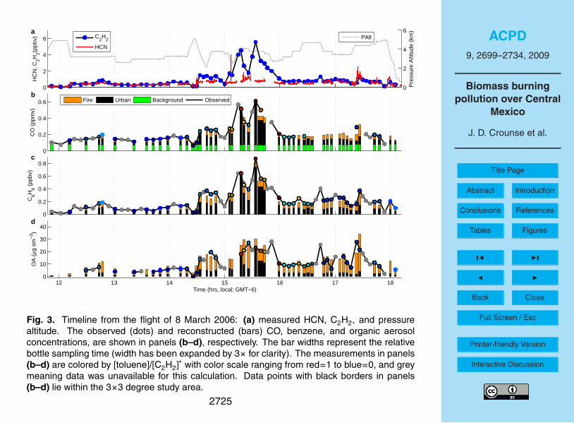
in Fig. 2, the sources of these gases within the basin are geographically (and tempo-rally) distinct and significant differences in their distribution can be observed on smallerspatial scales. This is illustrated in Fig. 3a. On 8 March 2006, the C-130 flew into15

the Mexico City basin and over a short period encountered air masses significantlyenhanced in either HCN, C2H2, or both (panel a).

To quantify the contribution of both fire and urban emissions to the distribution ofa trace gas (or aerosol), Y , we implement a simple two end-member model using themeasured excess HCN, [HCN]∗, and measured excess C2H2, [C2H2]∗, as tracers:20

Y = FY (fire) × [HCN]∗ + FY (urban) × [C2H2]∗ (1)

where,

[HCN]∗=[HCN]−SHCN(urban) × [C2H2]∗−[HCN]background (2)

[C2H2]∗=[C2H2]−SC2H2(fire) × [HCN]∗−[C2H2]background (3)

FY are scalars that relate the emission of Y from fire and urban sources to the emis-25

sions of HCN and C2H2, respectively (Table 1). SHCN and SC2H2are the emission ratios

2704





ACPD9, 2699–2734, 2009


Mexico


Title Page



Tables Figures

J I

J I

Back Close

Full Screen / Esc



of HCN to C2H2 and C2H2 to HCN for urban and fire emissions, respectively. Thesecross terms account for the contribution of urban and fire emissions to the excess HCNand C2H2, respectively. We also account for the amounts of these tracers advectedinto the region from afar (backgrounds).

Gasoline and diesel engine exhaust contain HCN, though previous measurements5

of the emissions vary by orders of magnitude (Baum et al., 2007). Automobiles lackingcatalytic converters can produce 100 times more HCN than automobiles with func-tional catalysts (Baum et al., 2007; Harvey et al., 1983). To estimate the appropriateemission ratio for Mexico City, SHCN, we use observations made from the C-130 on 29March when the C-130 sampled city emissions with what appears to be minimal fire10

influence (Fast et al., 2007). The measured slope of HCN to C2H2 in the city plumesencountered on this day is 0.054 (mol/mol). The ratio of CH3CN to HCN in the cityemissions is 0.5, similar to the ratio measured in both fire plumes and in the regionas a whole. This is in contrast to observations from Asia where urban emissions hada much lower ratio CH3CN to HCN (Li et al., 2003). Thus it is possible that even on15

the 29th, some of the HCN is from burning. Given our cross term corrections, andassuming urban fire sources such as garbage, coal, and biofuel burning was no dif-ferent on 29 March than on other days, emissions from these urban fire sources arecounted as urban emissions and not as fire emissions. Using the 0.054 (mol/mol) asan upper limit for the HCN/C2H2 emission ratio from urban emissions, we estimate that20

all urban emissions of HCN account for no more than 15% of the total emissions in thebasin during March 2006. Other sources of HCN from, for example, coal burning andpetrochemical industries are also estimated to be small (see Appendix A2).

We use measurements of C2H2 and HCN observed in forest fires in and aroundMexico City to estimate SC2H2

(Yokelson et al., 2007b). The emission of C2H2 from25

these forest fires was near the low end of the range typically observed for extratropicalforest fires (Yokelson et al., 2007b; Andreae and Merlet, 2001). We estimate that thecontribution of biomass burning to C2H2 accounts for less than 10% of the C2H2 in andaround Mexico City (see Table 1).

2705





ACPD9, 2699–2734, 2009


Mexico


Title Page



Tables Figures

J I

J I

Back Close

Full Screen / Esc



To account for the background amounts of C2H2 and HCN advected into to the re-gion, we use our observations in air sampled aloft, away from the Mexico City basin.We use separate HCN and C2H2 backgrounds for the gas phase species and for or-ganic aerosol/scattering, as aerosols have a more variable atmospheric lifetime. Forthe gas phase species (CO, benzene, and NOy), we use a constant value of 140 pptv for5

the background values of HCN for flights before 21 March. Following a shift in weatheron 21–22 March (Fast et al., 2007) (see also Figs. 10–12), we find higher backgroundconcentrations for HCN (220 pptv). C2H2 backgrounds are quite small (0–30 pptv), sowe have used a constant background value of 0 pptv for the analysis of the gas phasespecies. For organic aerosol and scattering, we have used a flight-by-flight analysis of10

the correlation of organic aerosol mass and scattering with HCN and C2H2 to definethe background HCN and C2H2. For flights in early March, the implied background ofHCN and C2H2 for organic aerosol (the abundance of these gases when the amountof organic aerosol is zero) is very close to the global backgrounds used in the analysisof the gases, but following the rainy period, 20–26 March, the apparent backgrounds15

for both HCN and C2H2 increased more drastically than for the gas phase pollutants;organic aerosol concentrations were near zero at significantly higher concentrations ofHCN and C2H2 (300 and 150 pptv, respectively). This difference is likely due to removalof aerosol (but not insoluble gases such as HCN, CO, C2H2, etc.) in the region duringthe rain storms.20

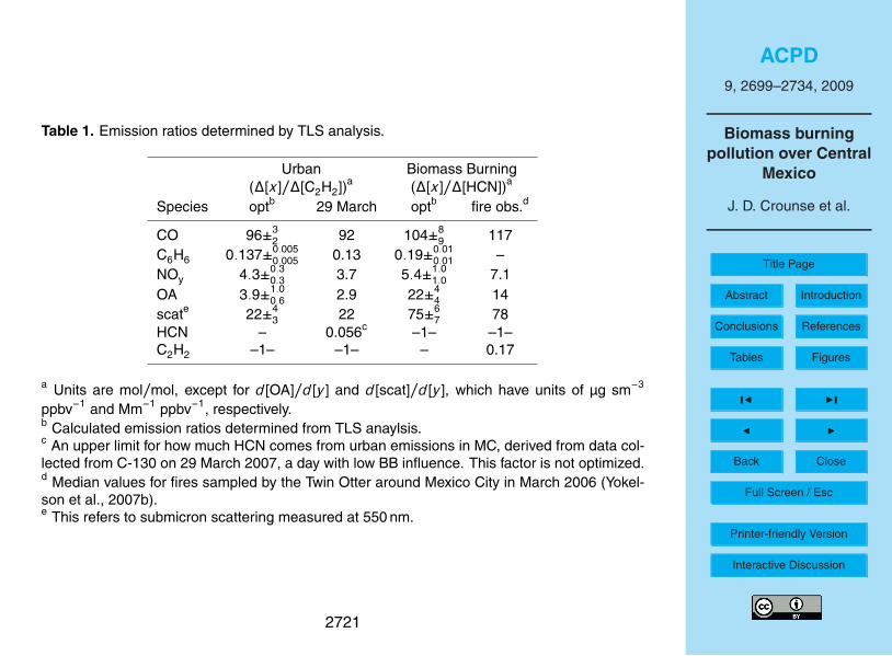
We derive a set of emission ratios, FY , for the pollutants using total least squares(TLS) analysis (Table 1). We weight [HCN]∗ and [C2H2]∗ by estimates of their errordetermined primarily from uncertainties in the backgrounds and in the variability ofthe emission ratios. We estimate the uncertainty in the derived emission ratios usinga bootstrap method (Efron and Tibshirani, 1993). The bootstrap method creates x25

alternate data sets by picking n random samples with replacement from the originaldata set, where n equals the number of samples in the original data set. The TLSanalysis is then performed across all alternate data sets, and statistics are computedon the results of all analyses. For this analysis we used x=1000. In Table 1, we also

2706





ACPD9, 2699–2734, 2009


Mexico


Title Page



Tables Figures

J I

J I

Back Close

Full Screen / Esc



summarize the emission factors determined independently from measurements madedirectly in biomass burning plumes measured in the basin during MILAGRO.

The variance in the abundance of our fire and urban tracers (HCN and C2H2) ex-plains most of the variability in CO and other pollutants. For example, in panels b,c, and d of Fig. 3, we show the observations (circles) for CO, benzene, and organic5

aerosol mass along the C-130 flight track. The observations are averaged to the sam-pling time of the whole air samples used to determine C2H2. The bars show the contri-butions from fire and urban emissions, estimated from [HCN]∗ (orange) and acetylene,[C2H2]∗ (black) using the emission ratios described in Table 1 and the mixing modeldescribed by Eq. (1).10

Figure 4a shows a scatter plot of the predictions from the two component modeland all observations made from the C-130 during MILAGRO for CO. The observationsmade within the 3×3 degree box surrounding MC are highlighted with a black border.CO has a relatively long lifetime in the atmosphere and there is a persistent north-ern hemispheric background of between 60 and 150 ppb that varies with season and15

latitude. To estimate the regional increase in [CO], we assume that the background[CO] is equal to the simulation of background CO taken from the Model for OZone AndRelated chemical Tracers (MOZART) chemical transport model (Horowitz et al., 2003),plus a constant 34 ppbv offset (see Fig. 3b, green bars). The offset was determinedfrom the bias between MOZART simulations and the observed CO in the cleanest air20

encountered during MILAGRO – typically aloft and outside the Mexico City basin. Fig-ure 4d shows the comparison for benzene. From the tracer analysis, we estimate thatbiomass burning accounts for (31±3)%, (36±3)%, and (34±7)% of the CO, benzene,and reactive nitrogen (NOy). These estimates are the mean of the mass-weighted,daily-averaged fire/excess fractions for observations made within the 3×3 degree box25

centered on MC, for the seven flights considered in this analysis. The sensitivity ofthese ratios to the size of the box is described in Table 2. Consistent with expectation,the fraction of pollution from biomass burning is lower for a smaller box centered overthe city.

2707





ACPD9, 2699–2734, 2009


Mexico


Title Page



Tables Figures

J I

J I

Back Close

Full Screen / Esc



Figure 5a shows a scatter plot of the predictions from the two component model fororganic aerosol. The data are colored by the ratio of toluene to acetylene. High ratios(red colors) are indicative of very fresh emissions with little photochemical processing.A similar figure for submicron aerosol scattering is shown as Fig. 8. From the traceranalysis, we estimate that biomass burning accounts for (66±11)%, and (57±5)% of5

the organic aerosol mass and total submicron scattering (which determines visibility).These estimates are the mean of the mass-weighted, daily-averaged fire/excess frac-tions for observations made within the 3×3 degree box centered on MC for the sevenflights considered in this analysis.

3 Discussion10

In Table 1, we compare the emission ratios estimated from the TLS analysis with ob-servations made in the city plume encountered on 29 March (little BB influence) andin fresh fire plumes sampled within the study area by the Twin Otter (Yokelson et al.,2007b). The derived emission ratios do not change when we exclude the data from the29th from the least-squares analysis.15

The urban ratio of CO to C2H2 measured on 29 March, 92 (mol/mol), is very closeto the emission ratio estimate from the total least squares (TLS) analysis, 96 (mol/mol)(Table 1). This ratio is lower than typically observed in US (300–500 mol/mol), andAsian cities (220 mol/mol) (Xiao et al., 2007), but comparable to the value observedby Grosjean et al. (1998) in urban air in Brazil. The lower emission ratios in Mexico20

and Brazil may reflect differences in fuel composition or catalytic converter function-ality (Sigsby et al., 1987). The relatively high concentration of C2H2 in traffic exhaustcombined with the emissions of C2H2 from fires near the low end of the typical rangemakes C2H2 a good tracer for the Mexican urban emissions.

The median ratio of CO to HCN observed in biomass burning plumes within the25

study area, 117 mol/mol (Yokelson et al., 2007b), is close to that derived in the totalleast-squares analysis, 104 mol/mol. As noted by Yokelson et al. (2007b), this ratio is

2708





ACPD9, 2699–2734, 2009


Mexico


Title Page



Tables Figures

J I

J I

Back Close

Full Screen / Esc



at the low end of the range typically observed for biomass burning. The relatively highemissions of HCN in biomass burning plumes combined with the low emission ratiosfrom urban sources makes HCN a very good tracer for biomass burning in Mexico City.

Biomass burning is a significant global source of benzene and the impact of thissource in and around the Mexico City basin is quite apparent in the correlations of5

benzene with the tracers (Fig. 4d–f). From the least squares analysis, we estimatethat fires contributed 36% of this pollutant to the atmosphere above the central Mex-ican Plateau in March 2006. Relative to CO, the benzene emission ratio for biomassburning derived here is similar to those reported in other studies (Andreae and Merlet,2001). As an aside, measurements of the ratio of benzene and toluene have been10

used in many previous studies to estimate the aging of an urban airmass as the at-mospheric oxidation of toluene occurs much more rapidly than benzene (e.g., Cubisonet al., 2006). Because the benzene/toluene emission ratio from fires (∼1–3) is muchgreater than the same emission ratio from urban emissions (0.2), this method is not ap-propriate for cities – such as Mexico City during the biomass burning season – which15

have significant contributions of benzene from fire emissions.Organic aerosol generally accounts for more than half the mass of fine particulate

matter (PM2.5) in (Salcedo et al., 2006) and around (DeCarlo et al., 2008) Mexico City.As shown in Fig. 5b–c, the amount of organic aerosol is highly correlated with [HCN]∗

and [C2H2]∗, suggestive of large fire and urban emission influences. Using the emission20

ratios described in Table 1, we estimate that biomass burning contributes 66% of theorganic aerosol to the study area in March 2006. These estimates are quite uncertain,however, due to complex aerosol chemistry.

Organic aerosol is both formed in and lost from the atmosphere on relatively fasttimescales. Although direct (or primary) emissions of organic aerosol from automobiles25

are quite small (∼5–10 µg per standard (T=273 K, P=1 atm) cubic meter of air (sm3)per ppmv CO), subsequent atmospheric oxidation of co-emitted hydrocarbons such astoluene and other aromatics, as well as biogenic and biomass burning hydrocarbonemissions, can yield low vapor pressure compounds that condense on the existing

2709





ACPD9, 2699–2734, 2009


Mexico


Title Page



Tables Figures

J I

J I

Back Close

Full Screen / Esc



particulate forming secondary organic aerosol (SOA) (Kroll and Seinfeld, 2008). Theamount of SOA produced from these gas-phase sources over the period of a day sub-stantially exceeds the primary emissions from urban sources (de Gouw et al., 2005;Kleinman et al., 2008; Robinson et al., 2007; Volkamer et al., 2006). The influence ofthis process is apparent in the aircraft data. In Fig. 5a, the organic aerosol data is col-5

ored by the ratio of toluene to acetylene. Toluene is co-emitted with acetylene in urbanemissions, but is oxidized in the atmosphere with a lifetime of approximately 12 daylighthours. In samples containing very high toluene (less oxidized), the total least-squaresanalysis tends to over-predict the amount of organic aerosol. For example, the urbanemission ratio derived from the least-squares analysis (∼39 µg per sm3 per ppmv CO10

or ∼3.9 µg per sm3 per ppbv of C2H2) is greater than the factor derived from the slopeof the correlations in the fresh plumes encountered on 29 March.

In addition to aerosol growth, aerosol mass can be lost through several mechanisms.As aerosol is transported away from its source and diluted with clean air, semi-volatilecompounds evaporate to the gas phase (Robinson et al., 2007). Dry and wet depo-15

sition also remove aerosol from the atmosphere. As mentioned earlier, the changingbackgrounds for aerosol relative to insoluble gases observed during late March is likelyexplained by aerosol loss via wet deposition.

Despite the complexity of the aerosol chemistry, the simple two end-member mixingmodel does describe much of the variability of organic aerosol mass observed from20

the C-130. This result may be related to our sampling – most of the observations weremade in the afternoon when the city and fire emissions had experienced some aging.The apparent organic aerosol emission ratio for urban emissions derived from the 29March plume, 32 µg OA per sm3 per ppmv CO, is not inconsistent with other estimatesfor organic aerosol from urban emissions aged 3–6 h (de Gouw et al., 2005; Volkamer25

et al., 2006). The aerosol burden continues to increase as the air masses are furtheroxidized in the MC outflow (Kleinman et al., 2008); similar to what has been observedin the New York City (de Gouw et al., 2005) and Atlanta plumes (Weber et al., 2007).

The complexity of the mixing of the urban-core aerosol emissions with the regional

2710





ACPD9, 2699–2734, 2009


Mexico


Title Page



Tables Figures

J I

J I

Back Close

Full Screen / Esc



aerosol emissions (often dominated by fire emissions) as well as mixing with the cleanfree troposphere precludes strong statements on the aerosol dynamics of these differ-ent sources.

The average NOx/VOC emission ratio for the fires surrounding Mexico City is similarto the urban NOx/VOC emission ratio for Mexico City. This is due in part to the higher5

than expected NOx emission from the fires, which is significantly (2–4 times) larger thantypical for fires (Yokelson et al., 2007b). As the fire and urban NOx/VOC emissions aresimilar, the fire emissions will significantly impact the ozone production in the MexicoCity outflow. Modeling of the transport and aging of the MC plume using a 3-D chem-ical transport model with full chemistry and accurate urban and fire emissions will be10

required to quantify the full impact of the fire emissions on ozone concentrations.

4 Implications for air quality improvement

The implications of this study for air quality engineering in Mexico City are not straightforward. Although visibility within the city and the export of aerosol, ozone, and othertrace gases is significantly impacted by biomass burning during the period of our ob-15

servations, it is not possible to estimate from this data set the long-term impact ofsuch burning on the urban dwellers of Mexico City. Biomass burning in March 2006was significantly higher than typical for March, though not unlike the amount of burn-ing usually observed in the height of the biomass burning in April/May. During mostof the year (June–February), however, these sources are negligible. Thus, annually-20

averaged, the impact of biomass burning will certainly be much smaller. In addition,because our sampling was from aircraft and primarily in the afternoon, and becausethe biomass burning was primarily in the forest above the city (Yokelson et al., 2007b),the impact of fire on the air breathed by people within Mexico City will be smaller thanthe regional impact estimated here. Indeed, we observe that even in the relatively well25

mixed afternoon planetary boundary layer, the impact of fire increases with altitude(Fig. 9). Consistent with this finding, estimates of the impact of fire on air quality at

2711





ACPD9, 2699–2734, 2009


Mexico


Title Page



Tables Figures

J I

J I

Back Close

Full Screen / Esc



the ground stations within the city suggest a smaller fire influence (Molina et al., 2007;Bravo et al., 2002; Salcedo et al., 2006; Yokelson et al., 2007b; Stone et al., 2008;Moffet et al., 2008). Finally, unlike reducing emissions from the urban sources, reduc-ing fire emissions through fire suppression efforts may have environmental costs aswell as benefits; although forest fire suppression in and around the basin would yield5

improvement in visibility, such fire suppression actions may be inconsistent with properforest management practices.

Appendix A

Additional information10

A1 Data sources

HCN was measured on the NCAR C-130 as discrete 0.5 s samples obtained every 5 s.The analysis was performed by chemical ionization mass spectrometry (Crounse et al.,2006). CH3CN was measured by a cryotrap concentrator coupled to a gas chromato-graph mass spectrometer (cryo-GCMS), an instrument similar to the one described by15

Apel et al. (2003). The cryo-GCMS instrument concentrated ambient air in the cryotrapfor 45 s prior to a 125 s analysis, yielding one data point every 170 s. C2H2, benzene,and toluene were recovered from 2 L canister samples that were periodically filled (ap-proximately 12 samples per hour for the flights into the city). Each canister is filledover a period of 30–120 s. These samples were analyzed by gas chromatography at20

UC-Irvine (Blake et al., 1997). NOy was measured by a chemiluminescence instrumentoperated by NCAR. Carbon monoxide was measured continuously with a vacuum ul-traviolet (VUV) fluorescence instrument similar to the one developed by Gerbig et al.(1999) with a precision of 3 ppbv and a typical accuracy of ±10% at 100 ppbv CO lev-els. On several flights, the VUV fluorescence CO measurements were not available25

and CO concentrations were determined from the canister samples. Aerosol composi-

2712





ACPD9, 2699–2734, 2009


Mexico


Title Page



Tables Figures

J I

J I

Back Close

Full Screen / Esc



tion (organic, sulfate, nitrate, ammonium, and chloride) and mass was determined witha high resolution aerosol mass spectrometer (DeCarlo et al., 2006, 2008). Aerosolscattering coefficients were measured at 450, 550, and 700 nm wavelengths using twoTSI-3563 nephelometers. One nephelometer measured submicron scattering employ-ing a 1 m aerodynamic impactor, and the other measured total scattering (Anderson5

et al., 2003).

A2 Alternative HCN sources

In addition to biomass burning and gasoline/diesel combustion, other sources of HCNmay contribute to the enhanced HCN in the basin. For example, HCN has also beenshown to be produced in the pyrolysis of coal from the breakdown of pyrrolic and pyri-10

dinic nitrogen (Leppalahti and Koljonen, 1995). Coal burning, however, is minimal in thebasin. According to the 1999 Mexico National Emissions Inventory (NEI), 88% of theCO produced in Mexico City, and surrounding states (summing over Distrito-Federal,Mexico, and Morales) comes from mobile sources (NEI, 2008).

We did observe elevated HCN in the plumes from the power plants (fuel-oil fired)15

and petrochemical complex in Tula, north of Mexico City. The ratio of HCN to CO in theTula plume is similar to that from fire. The Tula CO emissions are, however, significantlysmaller than the CO emissions from fire in the MC basin suggesting these emissionshave minimal influence on the regional HCN budget.

A3 HCN and acetonitrile correlation20

A reasonable correlation (r2=0.78, n=835) exists between HCN and CH3CN observa-tions, suggesting similar sources (Fig. 6). However, on multiple occasions, directly overMexico City, enhanced CH3CN was observed without accompanying enhancements inHCN (see Fig. 6, data excursions well above the best fit line). Explanations for theseCH3CN plumes could include industrial, non-combustion, sources, or possibly a differ-25

ent compound interfering with the GC-MS CH3CN measurement. Overall, ∆CH3CN is

2713





ACPD9, 2699–2734, 2009


Mexico


Title Page



Tables Figures

J I

J I

Back Close

Full Screen / Esc



39% of ∆HCN (Fig. 6). On 29 March, a day with little fire influence according to HCNlevels relative to CO, the slope of CH3CN to HCN is similar to the overall relationship,indicating that these compounds are emitted from urban sources in about the sameratio as from fire, or that fire is still the dominating source of these compounds even fordays without large fires.5

A4 NOy and submicron scattering

Analogous to Figs. 4 and 5, NOy (Fig. 7), and submicron scattering at 550 nm (Fig. 8)reconstructions are shown. The two component fit for total scattering yielded very sim-ilar results as the one for submicron scattering (e.g. fire fraction also equal to 57%),with similar correlation coefficients. Significant amounts of aerosol nitrate were mea-10

sured in and around Mexico City, so total NOy was taken as the sum of measuredNOy and aerosol nitrate. At this time it is not known what fraction of aerosol nitratewas sampled by the NOy instrument. To whatever extent aerosol nitrate is sampled bythe NOy instrument, we are double counting this aerosol nitrate. The correlation withthe 2-component model is significantly better if the aerosol nitrate is added to the NOy15

measurement to give total NOy.

A5 Altitude dependence of fire impact

As observed from the C-130, and inferred by comparing the C-130 data with observa-tions on the ground in Mexico City, the impact of the fires surrounding Mexico City isnot as severe on the ground, as it is above the City. This is due in part to the location20

of the fires, elevated above the city on the mountainsides surrounding the city. Theimpact of fire increases with altitude above Mexico City (Fig. 9), suggesting that thesmoke from the fires does not fully impact the ground.

2714





ACPD9, 2699–2734, 2009


Mexico


Title Page



Tables Figures

J I

J I

Back Close

Full Screen / Esc



A6 Box size for study area

For the ratios of fire impact reported in the body of the main work a rectangular studyarea of 3×3 degrees, centered on MC, was considered. As one focuses more on MCby decreasing the box size, the urban emissions become relatively more important (Ta-ble 2). This makes sense considering the fires emissions originate from many diffuse5

sources (individual fires) scattered across the plateau, while the urban emissions aremore centrally located in and around the MC basin. Table 2 compares the results forthe 2-component model using three different box sizes. Box 1 is the smallest, encom-passing the populated area of Mexico City and some adjacent terrain. Box 2 is largerand includes the ring of mountains around MC. Box 3 is the largest box, equating to10

the 3×3 degree box used for the results presented in the main body of this work.

A7 MODIS AQUA satellite image time line

A daily timeline of true color satellite images of the Mexico City area, collected from theMODIS instrument aboard the AQUA satellite, for the Month of March 2006 are shownin Figs. 10–12. The images were taken at approximately 1:30 p.m. local time each day.15

The red boxes on each satellite image represent detected thermal anomalies. One canobserve from inspection of the images that many fires are not detected due to a numberof reasons, including cloud cover, smoke cover, low fire temperature, or simply lack ofsatellite coverage. Also, the number of detected fires does not necessarily correlatewith the impact of fires on the visibility as observed from the satellite pictures.20

Acknowledgements. The MIRAGE-mex campaign was a cooperative project of NASA andNSF. Funding for Caltech was provided through NASA (NAG: NNG06GB32B). We thankS. Madonich, F. Flocke, and NCAR’s Research Aviation Facility (RAF) for mission design andsupport with instrument integration onto the aircraft. The National Center for AtmosphericResearch is sponsored by the National Science Foundation. C. Wiedinmyer provided clima-25

tological fire data from the MODIS instrumentation. We thank J. Fast for comments on thiswork. We thank U. Steiner, J. Oliver, and N. Allen for technical support of the CIMS instru-

2715





ACPD9, 2699–2734, 2009


Mexico


Title Page



Tables Figures

J I

J I

Back Close

Full Screen / Esc



ments whose development was generously supported by William and Sonja Davidow. J.D.C.and P.F.D. acknowledge support from the EPA-STAR Fellowship Program (FP916334012 andFP91650801). Funding for J.L.J. and P.D.F was provided though NSF (ATM-0513116) andNASA grants (NNG06GB03G). D.R.B. acknowledges NSF’s Atmospheric Chemistry Division(ACD) for support. This work has not been formally reviewed by the EPA. The views expressed5

in this document are solely those of the authors and the EPA does not endorse any products orcommercial services mentioned in this publication.

References

Anderson, T., Masonis, S., Covert, D., Ahlquist, N., Howell, S., Clarke, A., and McNaughton, C.:Variability of aerosol optical properties derived from in situ aircraft measurements during10

ACE-Asia, J. Geophys. Res.-Atmos., 108, 8647, doi:10.1029/2002JD003247, 2003. 2713Andreae, M. and Merlet, P.: Emission of trace gases and aerosols from biomass burning, Global

Biogeochem. Cy., 15, 955–966, 2001. 2705, 2709Apel, E., Hills, A., Lueb, R., Zindel, S., Eisele, S., and Riemer, D.: A fast-GC/MS system to

measure C-2 to C-4 carbonyls and methanol aboard aircraft, J. Geophys. Res.-Atmos., 108,15

8794, doi:10.1029/2002JD003199, 2003. 2712Baum, M. M., Moss, J. A., Pastel, S. H., and Poskrebyshev, G. A.: Hydrogen cyanide

exhaust emissions from in-use motor vehicles, Environ. Sci. Technol., 41, 857–862,doi:10.1021/es061402v, 2007. 2705

Blake, N., Blake, D., Chen, T., Collins, J., Sachse, G., Anderson, B., and Rowland, F.: Distri-20

bution and seasonality of selected hydrocarbons and halocarbons over the western Pacificbasin during PEM-West A and PEM-West B, J. Geophys. Res.-Atmos., 102, 28 315–28 331,1997. 2712

Bravo, A., Sosa, E., Sanchez, A., Jaimes, P., and Saavedra, R.: Impact of wildfires on the airquality of Mexico City, 1992–1999, Environ. Pollut., 117, 243–253, 2002. 2702, 271225

Crounse, J. D., McKinney, K. A., Kwan, A. J., and Wennberg, P. O.: Measurement of gas-phasehydroperoxides by chemical ionization mass spectrometry, Anal. Chem., 78, 6726–6732,doi:10.1021/ac0604235, 2006. 2712

Cubison, M. J., Alfarra, M. R., Allan, J., Bower, K. N., Coe, H., McFiggans, G. B., White-head, J. D., Williams, P. I., Zhang, Q., Jimenez, J. L., Hopkins, J., and Lee, J.: The char-30

2716





ACPD9, 2699–2734, 2009


Mexico


Title Page



Tables Figures

J I

J I

Back Close

Full Screen / Esc



acterisation of pollution aerosol in a changing photochemical environment, Atmos. Chem.Phys., 6, 5573–5588, 2006,http://www.atmos-chem-phys.net/6/5573/2006/. 2709

de Gouw, J., Middlebrook, A., Warneke, C., Goldan, P., Kuster, W., Roberts, J., Fehsen-feld, F., Worsnop, D., Canagaratna, M., Pszenny, A., Keene, W., Marchewka, M., Bert-5

man, S., and Bates, T.: Budget of organic carbon in a polluted atmosphere: Resultsfrom the New England Air Quality Study in 2002, J. Geophys. Res.-Atmos., 110, D16305,doi:10.1029/2004JD005623, 2005. 2710

DeCarlo, P. F., Kimmel, J. R., Trimborn, A., Northway, M. J., Jayne, J. T., Aiken, A. C., Go-nin, M., Fuhrer, K., Horvath, T., Docherty, K. S., Worsnop, D. R., and Jimenez, J. L.:10

Field-deployable, high-resolution, time-of-flight aerosol mass spectrometer, Anal. Chem., 78,8281–8289, doi:10.1021/ac061249n, 2006. 2713

DeCarlo, P. F., Dunlea, E. J., Kimmel, J. R., Aiken, A. C., Sueper, D., Crounse, J.,Wennberg, P. O., Emmons, L., Shinozuka, Y., Clarke, A., Zhou, J., Tomlinson, J.,Collins, D. R., Knapp, D., Weinheimer, A. J., Montzka, D. D., Campos, T., and Jimenez, J. L.:15

Fast airborne aerosol size and chemistry measurements above Mexico City and CentralMexico during the MILAGRO campaign, Atmos. Chem. Phys., 8, 4027–4048, 2008,http://www.atmos-chem-phys.net/8/4027/2008/. 2709, 2713

Efron, B. and Tibshirani, R.: An Introduction to the Bootstrap, Monogr. Stat. Appl. Probab., 57,1–177, 1993. 270620

Fast, J. D., de Foy, B., Acevedo Rosas, F., Caetano, E., Carmichael, G., Emmons, L.,McKenna, D., Mena, M., Skamarock, W., Tie, X., Coulter, R. L., Barnard, J. C., Wiedin-myer, C., and Madronich, S.: A meteorological overview of the MILAGRO field campaigns,Atmos. Chem. Phys., 7, 2233–2257, 2007,http://www.atmos-chem-phys.net/7/2233/2007/. 2702, 2705, 270625

Gerbig, C., Schmitgen, S., Kley, D., Volz-Thomas, A., Dewey, K., and Haaks, D.: An improvedfast-response vacuum-UV resonance fluorescence CO instrument, J. Geophys. Res.-Atmos.,104, 1699–1704, 1999. 2712

Giglio, L., Descloitres, J., Justice, C., and Kaufman, Y.: An enhanced contextual fire de-tection algorithm for MODIS, Remote Sens. Environ., 87, 273–282, doi:10.1016/S0034-30

4257(03)00184-6, 2003. 2702Grosjean, E., Grosjean, D., and Rasmussen, R.: Ambient concentrations, sources, emission

rates, and photochemical reactivity of C-2-C-10 hydrocarbons in Porto Alegre, Brazil, Envi-

2717





http://www.atmos-chem-phys.net/6/5573/2006/



ACPD9, 2699–2734, 2009


Mexico


Title Page



Tables Figures

J I

J I

Back Close

Full Screen / Esc



ron. Sci. Technol., 32, 2061–2069, 1998. 2708Harvey, C., Garbe, R., Baines, T., Somers, J., Hellman, K., and Carey, P.: A study of the

potential impact of some unregulated motor vehicle emissions, SAE Transactions, 92, 3–3,1983. 2705

Horowitz, L., Walters, S., Mauzerall, D., Emmons, L., Rasch, P., Granier, C., Tie, X., Lamar-5

que, J., Schultz, M., Tyndall, G., Orlando, J., and Brasseur, G.: A global simulation of tro-pospheric ozone and related tracers: Description and evaluation of MOZART, version 2, J.Geophys. Res.-Atmos., 108, 4784, doi:10.1029/2002JD002853, 2003. 2707

Kleinman, L. I., Springston, S. R., Daum, P. H., Lee, Y.-N., Nunnermacker, L. J., Senum, G. I.,Wang, J., Weinstein-Lloyd, J., Alexander, M. L., Hubbe, J., Ortega, J., Canagaratna, M. R.,10

and Jayne, J.: The time evolution of aerosol composition over the Mexico City plateau, At-mos. Chem. Phys., 8, 1559–1575, 2008,http://www.atmos-chem-phys.net/8/1559/2008/. 2710

Kroll, J. H. and Seinfeld, J. H.: Chemistry of secondary organic aerosol: Formation andevolution of low-volatility organics in the atmosphere, Atmos. Environ., 42, 3593–3624,15

doi:10.1016/j.atmosenv.2008.01.003, 2008. 2710Leppalahti, J. and Koljonen, T.: Nitrogen evolution from coal, peat and wood during gasification

– Literature-review, Fuel Process. Technol., 43, 1–45, 1995. 2713Li, Q., Jacob, D., Yantosca, R., Heald, C., Singh, H., Koike, M., Zhao, Y., Sachse, G., and

Streets, D.: A global three-dimensional model analysis of the atmospheric budgets of HCN20

and CH3CN: Constraints from aircraft and ground measurements, J. Geophys. Res.-Atmos.,108, 8827, doi:10.1029/2002JD003075, 2003. 2703, 2705

Lloyd, A.: California clean-air initiatives – The role of fuel cells, J. Power Sources, 37, 241–253,1992. 2701

McKinley, G., Zuk, M., Hojer, M., Avalos, M., Gonzalez, I., Iniestra, R., Laguna, I., Martinez, M.,25

Osnaya, P., Reynales, L., Valdes, R., and Martinez, J.: Quantification of local and globalbenefits from air pollution control in Mexico City, Environ. Sci. Technol., 39, 1954–1961,doi:10.1021/es035183e, 2005. 2702

Moffet, R. C., de Foy, B., Molina, L. T., Molina, M. J., and Prather, K. A.: Measurement of am-bient aerosols in northern Mexico City by single particle mass spectrometry, Atmos. Chem.30

Phys., 8, 4499–4516, 2008,http://www.atmos-chem-phys.net/8/4499/2008/. 2712

Molina, L. and Molina, M.: Air Quality in the Mexico Megacity: An Integrated Assessment,

2718







ACPD9, 2699–2734, 2009


Mexico


Title Page



Tables Figures

J I

J I

Back Close

Full Screen / Esc



Kluwer Academic Publishers, 2002. 2701Molina, L. T., Kolb, C. E., de Foy, B., Lamb, B. K., Brune, W. H., Jimenez, J. L., Ramos-

Villegas, R., Sarmiento, J., Paramo-Figueroa, V. H., Cardenas, B., Gutierrez-Avedoy, V., andMolina, M. J.: Air quality in North America’s most populous city – overview of the MCMA-2003 campaign, Atmos. Chem. Phys., 7, 2447–2473, 2007,5

http://www.atmos-chem-phys.net/7/2447/2007/. 2702, 2712Muhle, J., Lueker, T. J., Su, Y., Miller, B. R., Prather, K. A., and Weiss, R. F.: Trace gas and

particulate emissions from the 2003 southern California wildfires, J. Geophys. Res.-Atmos.,112, D03307, doi:10.1029/2006JD007350, 2007. 2702

NEI: Mexico National Emissions Inventory, 1999, http://www.epa.gov/ttn/chief/net/mexico/10

1999 mexico nei final report.pdf, 2008. 2713Ratcliff, M., Medley, E., and Simmonds, P.: Pyrolysis of amino-acids – Mechanistic considera-

tions, J. Org. Chem., 39, 1481–1490, 1974. 2703Robinson, A. L., Donahue, N. M., Shrivastava, M. K., Weitkamp, E. A., Sage, A. M.,

Grieshop, A. P., Lane, T. E., Pierce, J. R., and Pandis, S. N.: Rethinking organic15

aerosols: Semivolatile emissions and photochemical aging, Science, 315, 1259–1262,doi:10.1126/science.1133061, 2007. 2710

Salcedo, D., Onasch, T. B., Dzepina, K., Canagaratna, M. R., Zhang, Q., Huffman, J. A., De-Carlo, P. F., Jayne, J. T., Mortimer, P., Worsnop, D. R., Kolb, C. E., Johnson, K. S., Zu-beri, B., Marr, L. C., Volkamer, R., Molina, L. T., Molina, M. J., Cardenas, B., Bernabe, R. M.,20

Marquez, C., Gaffney, J. S., Marley, N. A., Laskin, A., Shutthanandan, V., Xie, Y., Brune, W.,Lesher, R., Shirley, T., and Jimenez, J. L.: Characterization of ambient aerosols in MexicoCity during the MCMA-2003 campaign with Aerosol Mass Spectrometry: results from theCENICA Supersite, Atmos. Chem. Phys., 6, 925–946, 2006,http://www.atmos-chem-phys.net/6/925/2006/. 2702, 2709, 271225

Sigsby, J., Tejada, S., Ray, W., Lang, J., and Duncan, J.: Volitile organic-compound emissionsfrom 46 in-use passenger cars, Environ. Sci. Technol., 21, 466–475, 1987. 2708

Singh, H., Salas, L., Herlth, D., Kolyer, R., Czech, E., Viezee, W., Li, Q., Jacob, D., Blake, D.,Sachse, G., Harward, C., Fuelberg, H., Kiley, C., Zhao, Y., and Kondo, Y.: In situ measure-ments of HCN and CH3CN over the Pacific Ocean: Sources, sinks, and budgets, J. Geophys.30

Res.-Atmos., 108, 8795, doi:10.1029/2002JD003006, 2003. 2703Solomon, S., Qin, D., Manning, M., Chen, Z., Marquis, M., Averyt, K., Tignor, M., and Miller, H.:

IPCC, 2007: Climate Change 2007: The Physical Science Basis. Contribution of Work-

2719






http://www.epa.gov/ttn/chief/net/mexico/1999_mexico_nei_final_report.pdf




ACPD9, 2699–2734, 2009


Mexico


Title Page



Tables Figures

J I

J I

Back Close

Full Screen / Esc



ing Group I to the Fourth Assessment Report of the Intergovernmental Panel on ClimateChange, 2007. 2701

Stone, E. A., Snyder, D. C., Sheesley, R. J., Sullivan, A. P., Weber, R. J., and Schauer, J. J.:Source apportionment of fine organic aerosol in Mexico City during the MILAGRO experi-ment 2006, Atmos. Chem. Phys., 8, 1249–1259, 2008,5

http://www.atmos-chem-phys.net/8/1249/2008/. 2712Volkamer, R., Jimenez, J. L., San Martini, F., Dzepina, K., Zhang, Q., Salcedo, D., Molina, L. T.,

Worsnop, D. R., and Molina, M. J.: Secondary organic aerosol formation from anthro-pogenic air pollution: Rapid and higher than expected, Geophys. Res. Lett., 33, L17811,doi:10.1029/2006GL026899, 2006. 271010

Weber, R. J., Sullivan, A. P., Peltier, R. E., Russell, A., Yan, B., Zheng, M., de Gouw, J.,Warneke, C., Brock, C., Holloway, J. S., Atlas, E. L., and Edgerton, E.: A study of secondaryorganic aerosol formation in the anthropogenic-influenced southeastern United States, J.Geophys. Res.-Atmos., 112, D13302, doi:10.1029/2007JD008408, 2007. 2710

WHO: Air Quality and Health, http://www.who.int/mediacentre/factsheets/fs313/en/index.html,15

2008. 2701Xiao, Y., Jacob, D. J., and Turquety, S.: Atmospheric acetylene and its relationship

with CO as an indicator of air mass age, J. Geophys. Res.-Atmos., 112, D12305,doi:10.1029/2006JD008268, 2007. 2708

Yokelson, R. J., Karl, T., Artaxo, P., Blake, D. R., Christian, T. J., Griffith, D. W. T., Guenther, A.,20

and Hao, W. M.: The Tropical Forest and Fire Emissions Experiment: overview and airbornefire emission factor measurements, Atmos. Chem. Phys., 7, 5175–5196, 2007a,http://www.atmos-chem-phys.net/7/5175/2007/. 2703

Yokelson, R. J., Urbanski, S. P., Atlas, E. L., Toohey, D. W., Alvarado, E. C., Crounse, J. D.,Wennberg, P. O., Fisher, M. E., Wold, C. E., Campos, T. L., Adachi, K., Buseck, P. R., and25

Hao, W. M.: Emissions from forest fires near Mexico City, Atmos. Chem. Phys., 7, 5569–5584, 2007b,http://www.atmos-chem-phys.net/7/5569/2007/. 2705, 2708, 2711, 2712, 2721

2720






http://www.who.int/mediacentre/factsheets/fs313/en/index.html



ACPD9, 2699–2734, 2009


Mexico


Title Page



Tables Figures

J I

J I

Back Close

Full Screen / Esc



Table 1. Emission ratios determined by TLS analysis.

Urban Biomass Burning(∆[x]/∆[C2H2])a (∆[x]/∆[HCN])a

Species optb 29 March optb fire obs.d

CO 96±32 92 104±8

9 117C6H6 0.137±0.005

0.005 0.13 0.19±0.010.01 –

NOy 4.3±0.30.3 3.7 5.4±1.0

1.0 7.1OA 3.9±1.0

0.6 2.9 22±44 14

scate 22±43 22 75±6

7 78HCN – 0.056c –1– –1–C2H2 –1– –1– – 0.17

a Units are mol/mol, except for d [OA]/d [y ] and d [scat]/d [y ], which have units of µg sm−3

ppbv−1 and Mm−1 ppbv−1, respectively.b Calculated emission ratios determined from TLS anaylsis.c An upper limit for how much HCN comes from urban emissions in MC, derived from data col-lected from C-130 on 29 March 2007, a day with low BB influence. This factor is not optimized.d Median values for fires sampled by the Twin Otter around Mexico City in March 2006 (Yokel-son et al., 2007b).e This refers to submicron scattering measured at 550 nm.

2721





ACPD9, 2699–2734, 2009


Mexico


Title Page



Tables Figures

J I

J I

Back Close

Full Screen / Esc



Table 2. Fire impact for pollutants considering several box sizes.

Species Box 1a (%) Box 2b (%) Box 3c (%)

CO 21 28 31C6H6 25 33 36NOy 24 31 34OA 52 61 66scat 43 52 57

a Box defined by latitude: [19.269 to 19.867] and longitude: [−99.300 to −98.867].b Box defined by latitude: [19.067 to 20.033] and longitude: [−99.433 to −98.667].c Box defined by latitude: [17.900 to 20.900] and longitude: [−100.400 to −97.400].

2722





ACPD9, 2699–2734, 2009


Mexico


Title Page



Tables Figures

J I

J I

Back Close

Full Screen / Esc



05−Mar−2006

Longitude (degrees)

Latit

ude

(deg

rees

)

a

−99.8 −99.6 −99.4 −99.2 −99 −98.8 −98.6 −98.418.5

19

19.5

20

10−Mar−2006

Longitude (degrees)

b

−99.8 −99.6 −99.4 −99.2 −99 −98.8 −98.6 −98.418.5

19

19.5

20

Fig. 1. MODIS-Aqua images of the Mexico City basin on (a) 5 March 2006 at 13:35 CSTand (b) 10 March 2006 at 13:55 CST, illustrate how large fires in the hillsides surrounding thecity can impact visibility. Red boxes are thermal anomalies detected by MODIS. Black linesrepresent Mexican state boundaries. Images courtesy of MODIS Rapid Response Project atNASA/GSFC.

2723





ACPD9, 2699–2734, 2009


Mexico


Title Page



Tables Figures

J I

J I

Back Close

Full Screen / Esc



Latit

ude

(deg

rees

)

HCNa−104 −102 −100 −98 −96 −94 −92 −90 −88

16

17

18

19

20

21

22

23

24

Latit

ude

(deg

rees

)

Longitude (degrees)

C2H

2b

−104 −102 −100 −98 −96 −94 −92 −90 −8816

17

18

19

20

21

22

23

24

0 0.25 0.5 0.75 1.0 1.25 >=1.5 C2H2(ppbv)

0 0.13 0.27 0.40 0.53 0.67 >=0.8 HCN(ppbv)

Fig. 2. C-130 flight tracks during MILAGRO colored by tracers: (a) observed HCN–HCNbackground, and (b) observed C2H2. The map has been divided into 0.2×0.2 degree pixelsand all observations from the C-130 across the MILAGRO campaign within a given pixel havebeen averaged together. High concentration data have been rounded down to capped valuesof 800 and 1500 ppbv for HCN and C2H2, respectively. Color scales range from 0 ppbv (darkblue) to the capped value (dark red). The black star in each panel is the center of Mexico City,and the black box outlines the 3×3 degree box centered on Mexico City which is the study areaconsidered for the fire impact analysis.

2724





ACPD9, 2699–2734, 2009


Mexico


Title Page



Tables Figures

J I

J I

Back Close

Full Screen / Esc



0

2

4

6H

CN

, C2H

2(ppb

v)

0

2

4

6

Pre

ssur

e A

ltitu

de (

km)

C2H

2

HCN

PAlt

0

0.2

0.4

0.6

CO

(pp

mv)

Fire Urban Background Observed

0

0.2

0.4

0.6

0.8

C6H

6 (pp

bv)

12 13 14 15 16 17 180

10

20

30

40

OA

(μg

sm

−3)

Time (hrs, local: GMT−6)

a

b

c

d

Fig. 3. Timeline from the flight of 8 March 2006: (a) measured HCN, C2H2, and pressurealtitude. The observed (dots) and reconstructed (bars) CO, benzene, and organic aerosolconcentrations, are shown in panels (b–d), respectively. The bar widths represent the relativebottle sampling time (width has been expanded by 3× for clarity). The measurements in panels(b–d) are colored by [toluene]/[C2H2]∗ with color scale ranging from red=1 to blue=0, and greymeaning data was unavailable for this calculation. Data points with black borders in panels(b–d) lie within the 3×3 degree study area.

2725





ACPD9, 2699–2734, 2009


Mexico


Title Page



Tables Figures

J I

J I

Back Close

Full Screen / Esc



0 0.1 0.2 0.3 0.4 0.5 0.6 0.7 0.80

0.1

0.2

0.3

0.4

0.5

0.6

0.7

0.8

0.9a

r2 = 0.98n = 497

Observed CO (ppmv)

Cal

cula

ted

CO

(pp

mv)

0

2

4

6

8b slope = 8.1

r2 = 0.94n = 497

Obs

erve

d C

2H2 (

ppbv

)

0 0.2 0.4 0.6 0.80

0.5

1

1.5c slope = 1.9

r2 = 0.25n = 497

Observed CO (ppmv)

Obs

erve

d H

CN

(pp

bv)

0 0.1 0.2 0.3 0.4 0.5 0.6 0.7 0.80

0.1

0.2

0.3

0.4

0.5

0.6

0.7

0.8

0.9d

r2 = 0.97n = 550

Observed benzene (ppbv)

Cal

cula

ted

benz

ene

(ppb

v)

0

2

4

6

8e slope = 4.7

r2 = 0.91n = 550

Obs

erve

d C

2H2 (

ppbv

)

0 0.2 0.4 0.6 0.80

0.5

1

1.5f slope = 1.4

r2 = 0.34n = 550

Observed benzene (ppbv)

Obs

erve

d H

CN

(pp

bv)

Fig. 4. Scatter plots for observed vs. reconstructed CO (a) and benzene (d). Associated scatterplots for CO vs. each tracer, [C2H2]∗ (b) and [HCN]∗ (c) and for benzene vs. each tracer, [C2H2]∗

(e) and [HCN]∗ (f). Lines are best fit to all data using total least squares (TLS) regression. Pointsare colored by [toluene]/[C2H2]∗, where red=1 and blue=0. Points with black border lie withinthe 3×3 degree study area.

2726





ACPD9, 2699–2734, 2009


Mexico


Title Page



Tables Figures

J I

J I

Back Close

Full Screen / Esc



0

5

10

15

20

25

30

35

Observed OA (μg sm−3)

Cal

cula

ted

OA

(μg

sm

−3)

ar2 = 0.89n = 270

0 10 20 30

0

2

4

6

8

Obs

erve

d C

2H2 (

ppbv

)

b slope = 0.08r2 = 0.54n = 270

0 10 20 300

0.5

1

1.5

Observed OA (μg sm−3)

Obs

erve

d H

CN

(pp

bv)

cslope = 0.026r2 = 0.67n = 270

Fig. 5. Scatter plot for observed vs. reconstructed OA (a). Associated scatter plots for OA vs.each tracer, [C2H2]∗ (b) and [HCN]∗ (c). Lines are best fit to all data using total least squares(TLS) regression. Points are colored by [toluene]/[C2H2]∗, where red=1 and blue=0. Pointswith black border lie within the 3×3 degree study area.

2727





ACPD9, 2699–2734, 2009


Mexico


Title Page



Tables Figures

J I

J I

Back Close

Full Screen / Esc



0 0.5 1 1.5 20

0.2

0.4

0.6

0.8

1

HCN (ppbv)

CH

3CN

(pp

bv)

Observations: n = 835; r2 = 0.78Least squares: slope = 0.45; int = 0.039Robust total least squares: slope = 0.39; int = 0.054

Fig. 6. Scatter plot of the HCN and the CH3CN observations made aboard the C-130 duringthe MILAGRO experiment (r2=0.78). The data (black x symbols) were fit using least squares(red: slope=0.45, intercept=0.039 ppbv), and robust total least squares (blue: slope=0.39,intercept=0.054) regression techniques.

2728





ACPD9, 2699–2734, 2009


Mexico


Title Page



Tables Figures

J I

J I

Back Close

Full Screen / Esc



0

10

20

30

40

50

Observed NOy (ppbv)

Cal

cula

ted

NO

y (p

pbv)

ar2 = 0.84n = 488

0 20 40

0

2

4

6

8

Obs

erve

d C

2H2 (

ppbv

)

b

slope = 0.15r2 = 0.81n = 488

0 20 400

0.5

1

1.5

Observed NOy (ppbv)

Obs

erve

d H

CN

(pp

bv)

c slope = 0.026r2 = 0.27n = 488

Fig. 7. Scatter plot for observed vs. reconstructed NOy (a). Associated scatter plots for NOy vs.each tracer, [C2H2]∗ (b) and [HCN]∗ (b). Lines are best fit to all data using total least squares(TLS) regression. Points are colored by [toluene]/[C2H2]∗, where red=1 and blue=0. Pointswith black border lie within the 3×3 degree study area.

2729





ACPD9, 2699–2734, 2009


Mexico


Title Page



Tables Figures

J I

J I

Back Close

Full Screen / Esc



0 0.05 0.1 0.15 0.20

0.05

0.1

0.15

0.2

ar2 = 0.88n = 526

Observed scattering (km−1)

Cal

cula

ted

scat

terin

g (k

m−1

)

0

2

4

6

8b

slope = 17.0r2 = 0.69n = 526

Obs

erve

d C

2H2 (

ppbv

)

0 0.05 0.1 0.150

0.5

1

1.5c slope = 6.9r2 = 0.54n = 526

Observed scattering (km−1)

Obs

erve

d H

CN

(pp

bv)

Fig. 8. Scatter plot for observed vs. reconstructed submicron scattering (a). Associated scatterplots for submicron scattering vs. each tracer, [C2H2]∗ (b) and [HCN]∗ (b). Lines are best fitto all data using total least squares (TLS) regression. Points are colored by [toluene]/[C2H2]∗,where red=1 and blue=0. Points with black border lie within the 3×3 degree study area.

2730





ACPD9, 2699–2734, 2009


Mexico


Title Page



Tables Figures

J I

J I

Back Close

Full Screen / Esc



0.1 0.2 0.3 0.4 0.5 0.61.5

2

2.5

3

3.5

4

4.5

5

5.5

FireCO

/(FireCO

+ UrbanCO

)

Pre

ssur

e al

titud

e (k

m)

Fig. 9. Altitude dependence of fire CO over Mexico City. The fraction of excess CO (CO-background) which according to the two component analysis comes from biomass burning vs.pressure altitude for observations (black x symbols) made within the 3×3 degree study areaaround Mexico City. Note the ground level in MC is at 2.2 km pressure altitude. The meanvalues of data for 1 km bins are shown as black circles connected by the red line.

2731





ACPD9, 2699–2734, 2009


Mexico


Title Page



Tables Figures

J I

J I

Back Close

Full Screen / Esc



05−Mar−2006

Latit

ude

−99.5 −99 −98.518.5

19

19.5

20

06−Mar−2006

−99.5 −99 −98.518.5

19

19.5

20

07−Mar−2006

−99.5 −99 −98.518.5

19

19.5

20

08−Mar−2006

Latit

ude

−99.5 −99 −98.518.5

19

19.5

20

09−Mar−2006

−99.5 −99 −98.518.5

19

19.5

20

10−Mar−2006

−99.5 −99 −98.518.5

19

19.5

20

11−Mar−2006

Longitude

Latit

ude

−99.5 −99 −98.518.5

19

19.5

20

12−Mar−2006

Longitude−99.5 −99 −98.5

18.5

19

19.5

20

13−Mar−2006

Longitude−99.5 −99 −98.5

18.5

19

19.5

20

Fig. 10. MODIS-Aqua images around Mexico City for 5 March through 13 March 2006. Redboxes represent detected fires. Black lines are state boundaries. Blank areas represent missingdata. Images courtesy of MODIS Rapid Response Project at NASA/GSFC.

2732





ACPD9, 2699–2734, 2009


Mexico


Title Page



Tables Figures

J I

J I

Back Close

Full Screen / Esc



14−Mar−2006

Latit

ude

−99.5 −99 −98.518.5

19

19.5

20

15−Mar−2006

−99.5 −99 −98.518.5

19

19.5

20

16−Mar−2006

−99.5 −99 −98.518.5

19

19.5

20

17−Mar−2006

Latit

ude

−99.5 −99 −98.518.5

19

19.5

20

18−Mar−2006

−99.5 −99 −98.518.5

19

19.5

20

19−Mar−2006

−99.5 −99 −98.518.5

19

19.5

20

20−Mar−2006

Longitude

Latit

ude

−99.5 −99 −98.518.5

19

19.5

20

21−Mar−2006

Longitude−99.5 −99 −98.5

18.5

19

19.5

20

22−Mar−2006

Longitude−99.5 −99 −98.5

18.5

19

19.5

20


2733





ACPD9, 2699–2734, 2009


Mexico


Title Page



Tables Figures

J I

J I

Back Close

Full Screen / Esc



23−Mar−2006

Latit

ude

−99.5 −99 −98.518.5

19

19.5

20

24−Mar−2006

−99.5 −99 −98.518.5

19

19.5

20

25−Mar−2006

−99.5 −99 −98.518.5

19

19.5

20

26−Mar−2006

Latit

ude

−99.5 −99 −98.518.5

19

19.5

20

27−Mar−2006

−99.5 −99 −98.518.5

19

19.5

20

28−Mar−2006

−99.5 −99 −98.518.5

19

19.5

20

29−Mar−2006

Longitude

Latit

ude

−99.5 −99 −98.518.5

19

19.5

20

30−Mar−2006

Longitude−99.5 −99 −98.5

18.5

19

19.5

20

31−Mar−2006

Longitude−99.5 −99 −98.5

18.5

19

19.5

20


2734





biomass burning and urban air pollution over the central ... · atmos. chem. phys. discuss., 9,...

Documents