Biological and physical controls on N2, O2 and CO2 distributions in 1

contrasting Southern Ocean surface waters 2

3

Philippe D. Tortell1,2, Henry C. Bittig3, Arne Körtzinger3, Elizabeth M. Jones4, 4

and Mario Hoppema4 5

6 1Department of Earth, Ocean and Atmospheric Sciences, University of British Columbia, 7

2207 Main Mall, Vancouver BC, Canada, V6T 1Z4. ptortell@eos.ubc.ca 8

2Department of Botany, University of British Columbia, 6270 University Blvd., 9

Vancouver BC, Canada, V6T 1Z4 10

3Marine Biogeochemistry, GEOMAR Helmholtz Centre for Ocean Research Kiel, 11

Düsternbrooker Weg 20, 24105 Kiel, Germany 12

4Alfred Wegener Institute, Helmholtz Centre for Polar and Marine Research, 13

Postfach 120161, 27515 Bremerhaven, Germany 14

15

16

Corresponding Author: Philippe D. Tortell, Dept. of Earth, Ocean and Atmospheric Sciences, 17

University of British Columbia, 2207 Main Mall, Vancouver BC, Canada, V6T 1Z4. 18

(ptortell@eos.ubc.ca) 19

20

21

22

Key Points: 23

Biological and physical controls on Southern Ocean gases are quantified 24

Sea-air CO2 fluxes significantly exceed regional climatological values 25

Net community production estimates are corrected for physical processes 26

Abstract: 27

We present measurements of pCO2, O2 concentration, biological oxygen saturation 28

(ΔO2/Ar) and N2 saturation (N2) in Southern Ocean surface waters during austral summer, 29

2010–2011. Phytoplankton biomass varied strongly across distinct hydrographic zones, with 30

high chlorophyll a (Chla) concentrations in regions of frontal mixing and sea-ice melt. pCO2 and 31

O2 /Ar exhibited large spatial gradients (range 90 to 450 atm and -10 to 60%, respectively) 32

and co-varied strongly with Chla. However, the ratio of biological O2 accumulation to dissolved 33

inorganic carbon (DIC) drawdown was significantly lower than expected from photosynthetic 34

stoichiometry, reflecting the differential time-scales of O2 and CO2 air-sea equilibration. We 35

measured significant oceanic CO2 uptake, with a mean air-sea flux (~ -10 mmol m-2 d-1) that 36

significantly exceeded regional climatological values. N2 was mostly supersaturated in surface 37

waters (mean N2 of +2.5 %), while physical processes resulted in both supersaturation and 38

undersaturation of mixed layer O2 (mean ΔO2phys = 2.1 %). Box model calculations were able to 39

reproduce much of the spatial variability of N2 and O2phys along the cruise track, 40

demonstrating significant effects of air-sea exchange processes (e.g. atmospheric pressure 41

changes and bubble injection) and mixed layer entrainment on surface gas disequilibria. Net 42

community production (NCP) derived from entrainment-corrected surface O2 /Ar data, ranged 43

from ~ -40 to > 300 mmol O2 m-2 d-1 and showed good coherence with independent NCP 44

estimates based on seasonal mixed layer DIC deficits. Elevated NCP was observed in 45

hydrographic frontal zones and stratified regions of sea-ice melt, reflecting physical controls on 46

surface water light fields and nutrient availability. 47

48

1. Introduction: 49 50

The Southern Ocean plays a key role in global nutrient and carbon cycles [Sarmiento et al., 51

2004; Schlitzer, 2002]. This vast region contributes significantly to oceanic CO2 uptake through 52

the vertical export of particulate organic carbon [Honjo et al., 2008; Schlitzer, 2002; Trull et al., 53

2001], and the subduction of CO2-rich polar water masses into the ocean interior [Caldeira and 54

Duffy, 2000; Sarmiento and Toggweiler, 1984]. These biological and physical carbon pumps 55

also transport oxygen and macro-nutrients into the low latitudes, where they influence biological 56

productivity over large spatial scales [Marinov et al., 2006; Sarmiento et al., 2004]. In the off-57

shore pelagic realm, Southern Ocean primary production and biological CO2 uptake appear to be 58

controlled by a combination of light and iron limitation [Boyd, 2002]. Large scale patterns of 59

aeolian iron deposition have been linked to spatial gradients in surface water productivity 60

[Cassar et al., 2007], while vertical mixing at frontal zones has been shown to drive mesoscale 61

and sub-mesoscale biological gradients [Sokolov and Rintoul, 2007]. Relative to the open ocean, 62

field data are sparse over much of the Antarctic continental shelf and marginal ice zone (MIZ), 63

where productivity is influenced by iron input from sediments [Coale et al., 2005; Planquette et 64

al., 2013] and melting ice [Gerringa et al., 2012; Sedwick and DiTullio, 1997], and by large 65

seasonal cycles in solar irradiance, mixed layer depth and sea ice cover [Arrigo and van Dijken, 66

2003]. Although these high latitude regions contribute disproportionately (on an areal basis) to 67

Southern Ocean nutrient and carbon cycles [Arrigo et al., 2008], their biological and physical 68

dynamics remain poorly described. 69

Here we present new results from a two-month survey of surface hydrography and dissolved 70

gas concentrations across the Atlantic sector of the Southern Ocean and the region west of the 71

Antarctic Peninsula. We use our observations to characterize the spatial variability of surface 72

gases in contrasting Southern Ocean regions (offshore pelagic, continental shelf and MIZ), and 73

to examine the relative influence of physical vs. biological controls on biogeochemical processes. 74

The interplay of physical and biological forcing is particularly important in determining surface 75

water pCO2 and O2 distributions. Net community production (NCP, i.e. gross photosynthesis 76

minus community respiration) leads to CO2 drawdown (i.e. decreased pCO2) in the mixed layer, 77

coupled with biologically-induced O2 supersaturation [Carrillo et al., 2004]. NCP is sensitive to 78

physical factors (e.g. wind speed, solar irradiance and ice cover) that control nutrient supply and 79

mixed layer light intensity. Physical processes also influence surface O2 and CO2 by modulating 80

the strength of diffusive air-sea exchange, which acts to restore gas concentrations back to 81

atmospheric equilibrium, and bubble processes, which lead to supersaturation of surface water 82

gases [Keeling, 1993]. Due to chemical buffering of the inorganic C system in seawater, the 83

diffusive air-sea equilibration time scale is typically ~ 10-fold slower for CO2 than for O2 84

[Sarmiento and Gruber, 2006], and gas exchange can thus overprint the biological production 85

signal, shifting the pCO2 – O2 relationship away from photosynthetic stoichiometry [Körtzinger 86

et al., 2008]. 87

Changes in surface water temperature and salinity can also influence O2 and CO2 88

distributions through their effect on gas solubility. For O2, these thermodynamic effects can be 89

removed by normalization to argon, a biologically inert gas with solubility properties that are 90

virtually identical to O2. The O2 /Ar ratio thus serves as a specific tracer for biological O2 cycling 91

[Craig and Hayward, 1987], and recent field measurements of O2/Ar disequilibrium (O2/Ar) 92

have been used to map the large-scale spatial distribution of NCP in Southern Ocean surface 93

waters [Cassar et al., 2011; Castro-Morales et al., 2013; Reuer et al., 2007; Shadwick et al., 94

2014; Tortell and Long, 2009]. NCP estimates derived from O2/Ar measurements are based on 95

a steady-state mixed layer model [Kaiser et al., 2005; Reuer et al., 2007], where vertical and 96

lateral exchange of O2 into the mixed layer is assumed to be negligible and NCP can thus be 97

equated to the biologically induced sea-air flux of O2 (O2-bioflux). These assumptions are likely 98

invalid over significant portions of the Southern Ocean, where vertical entrainment of 99

biologically modified sub-surface waters leads to significant uncertainty in derived mixed layer 100

NCP values [Jonsson et al., 2013]. Better constraints on the physical contributions to mixed 101

layer O2 mass balance are thus needed to improve the use of O2/Ar as a productivity tracer. 102

Like Ar, N2 is biologically inert in the Southern Ocean, where nitrogen fixation and 103

denitrification are inhibited by high NO3- and O2 concentrations, respectively. Given the high 104

atmospheric concentrations of N2 and its relatively low solubility in seawater, this gas provides a 105

useful tracer for air-sea exchange processes, including bubble injection [Schudlich and Emerson, 106

1996]. A number of studies have used surface ocean N2 disequilibrium measurements (N2) to 107

examine air-sea exchange [Emerson et al., 2002; Hamme and Emerson, 2006; Vagle et al., 108

2010], and a mechanistic framework has recently been developed to quantitatively interpret 109

surface N2 data [Liang et al., 2013; Nicholson et al., 2008; Nicholson et al., 2011; Stanley et al., 110

2009]. At present, we are aware of only one published N2 data set from Southern Ocean waters 111

[Weeding and Trull, 2014]. Additional N2 measurements from this region are thus needed to 112

validate the model-based calculations under conditions of high wind-speeds, strong gradients in 113

atmospheric pressure and significant bubble injection fluxes. 114

Using simultaneous measurements of N2, O2, O2/Ar and CO2, in combination with 115

ancillary data and box model calculations, we examined the dominant controls on surface gas 116

saturation states in contrasting Southern Ocean surface waters. Our results provide insight into 117

the factors driving gas dynamics in various sub-regions of the Southern Ocean, demonstrating 118

clear regional differences in the relative importance of physical and biological forcing. Our 119

observations reveal strong biological controls on surface CO2 and O2 distributions, with a 120

significant imprint of air-sea exchange. Using box model calculations, we show that the 121

formulation of Nicholson et al. [2011] is able to provide reasonable estimates of physically-122

induced changes in O2 and N2 saturation states, and we derive NCP estimates that are corrected 123

for entrainment of biologically modified sub-surface waters into the mixed layer. Our work 124

builds on the recent study of Shadwick et al. [2014] examining CO2, O2 and O2 /Ar along a 125

transect south of Australia, and Weeding and Trull [2014], who present a mooring-based O2 and 126

N2 time-series for the Subantarctic region south of Tasmania. To our knowledge, our work 127

represents the first simultaneous measurements of pCO2, O2, O2 /Ar and N2 for the Southern 128

Ocean, and we show how these combined observations can provide powerful insights into 129

surface water biogeochemical processes across a range of hydrographic regimes. 130

131

2. Methods: 132

133

2.1 Study site and hydrographic measurements 134

We conducted a 10-week survey of Southern Ocean waters from Nov. 29, 2010 to Feb. 3, 135

2011 on board the research vessel Polarstern (cruise ANT-XXVII/2; [Rohardt, 2011]). Our 136

cruise track from Cape Town, South Africa, to Punta Arenas, Chile (Figure 1) encompassed a 137

number of distinct hydrographic regimes. For the purposes of our analysis, we separate the 138

cruise track into three sub-regions. We first sampled a N-S transect ~ 40˚S to 70˚S, crossing a 139

number of prominent hydrographic fronts [Orsi et al., 1995], including the Subtropical Front 140

(STF), Sub-Antarctic Front (SAF), Polar Front (PF), Southern Antarctic Circumpolar Current 141

Front (SACCF) and Southern Boundary of the Antarctic Circumpolar Current (SBdy). We then 142

followed an E-W transect along the outer edge of the Weddell Sea MIZ, and conducted an 143

intensive survey of the West Antarctic Peninsula (WAP) along the Palmer Long Term Ecological 144

Research (LTER) sampling grid [Waters and Smith, 1992]. 145

Sea surface temperature (SST) and salinity (SSS) were measured continuously along the 146

cruise track using an on-board thermosalinograph (TSG; Sea-Bird Electronics, model SBE-21) 147

sampling from an uncontaminated seawater supply with a nominal intake depth of 11 m. Daily 148

calibrations of the TSG salinity measurements were conducted using discrete samples analyzed 149

on a salinometer (Optimare GmbH, Precision Salinometer). Sea surface Chla fluorescence, used 150

as a proxy for bulk phytoplankton biomass, was continuously measured by the ship’s underway 151

fluorometer (WET labs, ECO). The fluorometer data were not calibrated to absolute Chla 152

concentrations and are thus used here only as a relative measure of total phytoplankton 153

abundance. Some day-time non-photochemical quenching of Chla fluorescence is expected, 154

independent of changes in phytoplankton biomass. 155

Depth profiles of seawater potential temperature, salinity and Chla fluorescence were 156

obtained from CTD casts at 188 stations along the cruise track. Temperature and conductivity 157

were measured with Sea-Bird SBE3plus and SBE4 sensors, respectively, while Chla 158

fluorescence was measured with a WET labs ECO fluorometer. Temperature and salinity profiles 159

were used to define the mixed layer depth for each station based on the curvature of near surface 160

layer density or temperature profiles as described by Lorbacher et al. [2006]. Mixed layer 161

temperature and salinity data derived from CTD casts showed very good agreement with surface 162

TSG data (mean offset of −0.078 ˚C and −0.01, respectively). The concentration of O2 in depth 163

profiles was measured using a CTD-mounted Sea-Bird SBE43 sensor. The CTD O2 sensor was 164

calibrated using Winkler titrations of discrete samples, with visual endpoint determination using 165

a starch indicator (precision of 0.3 μmol L-1) and KIO3 standardization of the thiosulfate titration 166

solutions [Dickson, 1994]. All of the CTD sensors were sent to the manufacturer for calibration 167

prior to and immediately after the cruise. Full quality-controlled hydrographic data from the 168

cruise are available in the Pangaea database (www.pangaea.de). 169

170

2.2 Surface water gas measurements 171

Surface pCO2 and O2 /Ar ratios were measured every ~ 30 s from the keel intake supply 172

using membrane inlet mass spectrometry (MIMS), following the protocols described by Tortell 173

et al. [2011]. At typical cruising speeds of 8–10 knots, this sampling frequency translates into 174

one measurement every ~ 200 m along the cruise track. The pCO2 measurements were 175

calibrated using temperature-controlled seawater standards [Tortell et al., 2011], and the 176

resulting pCO2 data were corrected to in situ SST following [Takahashi et al., 2002]. Note that 177

pCO2 data are not available for much of the N-S transect due to instrument problems. O2 /Ar 178

measurements in the flow-through seawater, (O2 /Ar)meas, were normalized to values measured 179

every few hours in air-equilibrated, temperature-controlled seawater standards, (O2 /Ar)sat. 180

[Tortell et al., 2011], to derive a biological O2 saturation term, O2 /Ar, expressed in % deviation 181

from equilibrium. 182

This term was calculated as [Craig and Hayward, 1987]: 183

O2 /Ar = [(O2 /Ar)meas / (O2 /Ar)sat -1] * 100 (1) 184

185

Surface O2 concentration measurements were made using an optode (Aanderaa Data 186

Instruments, model 3830), while total gas pressure (mbar) was measured using a gas tension 187

device (Pro-Oceanus, model HGTD). The gas tension device was not functional during the latter 188

half of the cruise. Both the optode and HGTD were submerged in a thermally insulated flow-189

through box connected to the keel seawater intake supply, and set to acquire data with a 1 min 190

resolution (close to the response time of the HGTD). The optode O2 measurements were 191

calibrated against CTD-O2 data, and cross validated against discrete Winkler titrations. The O2 192

saturation state (O2; % deviation from equilibrium) was derived from measured O2 193

concentrations and an equilibrium O2 concentration computed from surface water temperature, 194

salinity and atmospheric pressure with the solubility function of Garcia & Gordon [1992]. Using 195

our optode and MIMS data, we derived an estimate of the physical contribution to O2 196

disequilibria in surface waters, O2phys. 197

198

O2phys = O2optode – O2 /ArMIMS (2) 199

The rationale for this approach is that optode-based O2 is sensitive to both physical and 200

biological influences, whereas MIMS-based O2 /Ar reflects only the biological contribution to 201

O2 disequilibria [Craig and Hayward, 1987], after normalizing for physical effects using the 202

biologically inert analog, argon. As calculated here (2), O2phys is thus functionally equivalent to 203

the physically-induced changes in Argon saturation, Ar. 204

Following the approach of McNeil et al. [McNeil et al., 2005; McNeil et al., 1995], we 205

derived estimates of N2 partial pressure from GTD total gas pressure by subtracting the partial 206

pressures of O2 (derived from optode measurements), water vapour (calculated from SST and 207

SSS) and Ar. 208

209

pN2 pTotal – pO2

– pH2O – pAr (3)

210

211

In previous studies, seawater Ar concentrations have been assumed to be at atmospheric 212

equilibrium values. This assumption contributes only a small uncertainty (< 0.1%) to the 213

calculation of N2 concentrations [McNeil et al., 1995], since Ar is a minor constituent of total 214

partial pressure and varies by only a few percent. Indeed, we observed a negligible difference 215

between pN2 calculated assuming 100% Ar saturation and calculations that included a specific 216

Ar term (derived from O2phys). Similarly, the inclusion of pCO2 into the calculation did not 217

have a significant effect on the resulting pN2. The N2 saturation state (N2) was calculated from 218

GTD-derived N2 concentrations and observed atmospheric pressure using the SST and salinity-219

dependent N2 solubility constant of Hamme and Emmerson [2004]. 220

221

2.3 Ancillary data 222

Ancillary meteorological and oceanographic data from a number of sources were used to 223

provide a broader environmental context for our observations, and input data for model 224

calculations (see below). Instantaneous measurements of sea level atmospheric pressure, wind 225

speed (corrected to 10 m above sea level) and solar irradiance were obtained from weather 226

station sensors on board the research vessel. Additional synoptic data on wind speed, sea level 227

atmospheric pressure and humidity were obtained from the NCEP reanalysis 228

(http://www.esrl.noaa.gov/psd/data/reanalysis/reanalysis.shtml) at 2.5˚ and 6 h resolution, while 229

regional SST information was derived from NOAA OISST (http://www.ncdc.noaa.gov/sst/) at 230

0.25˚ and 24 h resolution. The NCEP wind speed data showed reasonably good agreement with 231

the instantaneous ship-board measurements (r = 0.78, RMSE = 2.9 m s-1). Although there was a 232

slight offset towards lower wind speeds in the NCEP data, the mean difference (-0.94 m s-1 ± 233

3.11) was not significantly different from zero. Sea ice data (% cover) at 3 km and 24 h 234

resolution were derived from AMSR-E satellite imagery using the ASI re-processing algorithm 235

provided by the Institute of Environmental Physics at the University of Bremen, Germany 236

[Spreen et al., 2008]. Regional sea surface salinity was obtained from the Mercator global 237

operational system PSY3V3 model at 0.25˚ and 24 h resolution (http://www.mercator-238

ocean.fr/eng/produits-services/Reference-products#tps_differe). Surface Chla concentrations 239

were obtained from Level 3 AquaModis satellite data (http://oceancolor.gsfc.nasa.gov/cgi/l3). 240

We used 9 km resolution imagery, with 8-day composite data linearly interpolated to daily 241

values. 242

243

2.4 CO2 flux calculations 244

Surface gas measurements and wind-speed data were used to derive sea-air flux estimates 245

for CO2. The CO2 fluxes were calculated as: 246

247

FCO2 = kCO2

αCO2

pCO2sw − pCO2atm) (1 − A)0.4 (4) 248

249

where kCO2 is the gas transfer velocity (m d−1), calculated from wind speed data and the 250

temperature-dependent Schmidt number using the parameterization of Sweeney et al. [2007], 251

αCO2

is the temperature and salinity-dependent solubility of CO2 [Weiss, 1974] and A is the 252

fraction of sea surface covered by ice. The exponential term used to scale gas exchange as a 253

function of ice cover is derived from Loose et al. [2009]. For these flux calculations, we used an 254

atmospheric CO2 mole fraction of 396 ppmv, derived from the GlobalView pCO2 data 255

(www.esrl.noaa.gov/gmd/ccgg/globalview/; 60˚S to 70˚S, Dec. 2010 - Feb. 2011), corrected to 256

100% humidity at SST and SSS and the atmospheric pressure derived from ship-based sensors. 257

Wind speeds used for the flux calculations were derived from one week averages of the NCEP 258

reanalysis product, matched to the ship's position along the cruise track. 259

260

2.5 Carbonate system measurements and calculations 261

Discrete samples for carbonate system measurements were collected at selected stations 262

along the cruise track using 12 L Niskin bottles mounted on the CTD rosette. Total alkalinity 263

was measured using potentiometric gran titration [Brewer et al., 1986], calibrated against 264

certified reference material (batches 100 and 105) supplied by Dr. Andrew Dickson, Scripps 265

Institution of Oceanography [Dickson et al., 2007]. The precision of the alkalinity measurements 266

was 1.5 mol kg-1. Seawater (500 mL) for DIC analysis was collected in borosilicate glass 267

bottles and analysed within 20 hours using a VINDTA 3C instrument (Versatile INstrument for 268

the Determination of Total Alkalinity, Marianda, Kiel). The DIC concentration was determined 269

by coulometric analysis [Johnson et al., 1987], with calibration against certified reference 270

materials (CRM, batches 100 and 105) performed at the start and end of each measurement 271

cycle. The precision of the DIC measurements was 1.0 μmol kg-1, based on the average 272

difference between all CRM in-bottle duplicate analyses (n 87), and the accuracy was 273

estimated as 2.0 μmol kg-1. 274

Depth-integrated DIC deficits were calculated from vertical profiles relative to the 275

concentration at the depth of the potential temperature minimum, representing the Winter Water. 276

The depth of the potential temperature minimum was determined from the CTD profiles. Vertical 277

integration to the potential temperature minimum was used to derive the chemical deficits in the 278

summer surface layer. DIC data were normalized to average Winter Water salinity (34.2, n 279

105) to account for dilution through addition of sea ice melt water. The chemical deficits, 280

calculated in this way, represent the time-integrated change of the surface ocean since the end of 281

the winter. This technique assumes that DIC concentrations at the potential temperature 282

minimum represent the winter reference with no significant lateral or vertical exchange. This 283

assumption has been used in prior studies [Hoppema et al., 2007; Jennings et al., 1984; Rubin et 284

al., 1998] and appears to be reasonably robust for the Weddell Sea [Hoppema et al., 2000b]. 285

In order to obtain high spatial resolution surface carbonate system data along the cruise 286

track, we derived an empirical linear relationship between salinity and alkalinity along the E-W 287

and WAP transects (n = 2098, r2 > 0.85, root mean square error = 6.1 mol kg-1), and used this 288

relationship to compute alkalinity from thermosalinograph salinity measurements. Total 289

dissolved inorganic carbon (DIC) along the cruise track was then computed from measured pCO2 290

and the derived alkalinity using CO2SYS [Pierrot et al., 2006], with the equilibrium constants of 291

Mehrbach et al., [1973] refit by Dickson and Millero [1987]. For the WAP and Weddell regions, 292

the root mean square error of the DIC estimates derived from this analysis was 7.1 and 3.8 mol 293

kg-1, respectively. This error term was based on a comparison of DIC values obtained using 294

measured vs. empirically-derived alkalinity. 295

296

2.6 Box model calculations 297

Following the work of Emerson et al. [2008] and Nicholson et al. [2011], we used a simple 298

box model to assess the physical contributions to N2 and O2 disequilibria in the mixed layer. The 299

1-D model includes an air-sea gas exchange term, Fas and a sub-surface water entrainment term, 300

Fentr, associated with mixed layer deepening events. Lateral and vertical advection, and vertical 301

diffusive mixing were assumed to be negligible, and no biological production / consumption 302

term was included in order to isolate physical forcing. For a given gas, x, the change in mixed 303

layer concentrations, dcx, was computed as: 304

305

mld dcx / dt = Fas,x + Fentr,x (5) 306

307

where mld is mixed layer depth. The air-sea flux term, Fas, was separated into several 308

components; diffusive gas exchange, Fdif, injection of small bubbles, Finj, and air-water interface 309

exchange across larger bubble surfaces, Fex. These gas exchange terms were all scaled to the 310

fraction of open water, A, following Loose et al. (2009), as described in section 2.4. The total 311

air-sea flux term (Fas) for gas x was thus computed as: 312

313

Fas,x = (Fdif,x + Finj,x + Fex,x ) (1 – A)0.4 (6) 314

315

Fdif,x = −kx (cx – αx px) (7) 316

317

Finj,x = Ainj px (u10 – 2.27)3 (8) 318

319

Fex,x = Aex px (Dx / 1 m2 s-1)0.5 (αx / 1 mol m-3 atm-1) (u10 – 2.27)3 (9) 320

321

where kx is the gas transfer velocity (m s-1) calculated following Sweeney et al. [2007], αx 322

the solubility (mol m-3 atm-1), px the partial pressure calculated from the mole fraction in dry air 323

and the dry atmospheric pressure (px = χx patm,dry), and Dx the diffusion coefficient (m2 s-1). The 324

injection and exchange rates Ainj and Aex (mol s2 m−5 atm−1) given in Nicholson et al. [2011] were 325

derived for average wind speeds. For our calculations based on short-term wind-speeds, we use 326

a flux enhancement factor, R, of 1.5 as discussed in Nicholson et al. [2011]. The bubble fluxes 327

Finj and Fex scale with whitecap coverage (0 for u10 < 2.27). 328

The entrainment term is governed by the change in mixed layer depth (only deepening of 329

the mixed layer impacts the surface water budget), and by difference between mixed layer 330

concentration cx and the concentration in the sub-surface layer cx,sub: 331

332

Fentr = (cx,sub – cx) d(mld) / dt (10) 333

334

The changes in mixed layer depth used to quantify the physical entrainment term were 335

obtained from temperature and salinity profiles of the Mercator global operational system 336

PSY3V3. These model-derived mixed layer depths, which assimilate all available measurements 337

in a given study region, showed reasonable agreement with values obtained from our actual CTD 338

observations (r = 0.61), and were able to reproduce the spatial patterns in mixing depths across 339

our cruise track (Fig. S1). Moreover, comparison of the time-dependent model MLD history, 340

with observations derived from Argo float data showed that the model output was able to 341

reproduce the significant changes in MLD (including a number of pronounced deepening events) 342

observed across our study region (Fig. S2). 343

For N2, the choice of the sub-mixed layer concentration cN2,sub has a minor influence on the 344

calculation given the weak vertical gradients of this gas in the absence of a sub-surface 345

biological production or consumption term. We thus chose a uniform value of 100 % surface 346

saturation for cN2,sub. In the case of O2, however, strong vertical gradients and variable saturation 347

levels have a significant influence on the entrainment term, and the choice of cO2,sub values can 348

thus exert a significant influence on the model calculations under conditions of mixed layer 349

deepening. Given our interest in comparing physical and biological processes affecting the 350

surface water O2 balance, we computed two different O2 entrainment terms. The first term, 351

O2pe, reflects the entrainment of sub-surface waters in the absence of a biological signature. 352

For this calculations the sub-surface O2 end-member (cO2,sub) was set to 100 %, as in the N2 353

calculations. We also computed a total O2 entrainment term, O2te, which reflects the bulk 354

transport of O2 into the mixed layer, based on the observed difference in O2 concentrations 355

between surface and sub-surface waters. For these calculations, we used the average O2 356

concentration 20 – 25 m below the mixed layer depth to define the end member concentration 357

(cO2,sub) for entrained waters. This depth was chosen based on examination of mixed layer depth 358

history from the PSY3V3 output during a number of modelled entrainment events. The mean 359

cO2,sub end member values were calculated from CTD data for each sampling station, and 360

interpolated to the full resolution of our cruise track for use in the entrainment calculations. 361

The model mixed layer concentrations of O2 and N2 were initialized at 100 % saturation 362

starting 30 d prior to the underway measurements. The ancillary data (e.g. wind speed, 363

atmospheric pressure, mixed layer depth etc.) were interpolated to the cruise track position and 364

time, and used to force the model calculations for 30 d with time-steps of 6 h. 365

366

2.7 Net community production estimates 367

We used the approach of Reuer et al. [2007] to estimate net community production (NCP, 368

i.e. gross photosynthesis minus community respiration) from our mixed layer O2 /Ar 369

measurements. The calculations presented by Reuer et al. [2007] are based on a steady-state 370

model, where lateral advection and vertical entrainment are assumed to be negligible, and the 371

mixed layer O2 mass balance is influenced solely by NCP and gas exchange. Under these 372

conditions, steady-state NCP is equivalent to the air-sea flux of biogenic O2 (obtained from O2 373

/Ar and the air-equilibrium O2 concentration, αO2

* patm). The gas exchange term, k, is derived 374

using a weighting function to account for variability in wind speed history over the residence 375

time of O2 in the mixed layer (see Reuer et al. [2007] for details). 376

377

NCP = O2 /Ar * αO2

* patm * k (11) 378

379

For consistency with our box model calculations, we used the gas exchange parameterization (k) 380

of Sweeney et al. [2007], and the ice-dependent scaling factor of Loose et al. [2009] to derived 381

NCP estimates. 382

We recognize that the assumptions required for the O2 /Ar-based NCP calculations are 383

unrealistic for at least some portions of our cruise track where entrainment of sub-surface waters 384

into the mixed layer is likely non-negligible. To examine the influence of mixed layer 385

entrainment on NCP, we used the output from our box model calculations (see above) to estimate 386

the O2 flux associated with changes in mixed layer depth. Based on our calculation of O2pe and 387

O2te, we derived a specific biological entrainment term, O2be, for use in the correction of O2 388

/Ar for NCP calculations. 389

390

O2be = O2te - O2pe (12) 391

392

This term reflects the entrainment of biologically-modified O2 signatures from sub-surface 393

waters. The purely physical entrainment term, O2pe, affects O2 and Ar in a nearly identical 394

manner, and thus has a negligible influence on the measured O2 /Ar ratio. In contrast, O2be 395

specifically affects O2, and thus modifies O2 /Ar. Our approach, based on the separation of 396

biogenic and non-biogenic entrainment fluxes thus allows us to correct the observed O2 /Ar 397

values for entrainment of biologically-modified sub-surface waters, after removing the non-398

biological entrainment signature. We used the corrected O2 /Ar data as input to equation 11. 399

Given the physical complexity of our study region, and its high degree of temporal variability, 400

we treat our NCP calculations as a first order estimate of biological O2 production rates in the 401

mixed layer, recognizing the quantitative limitations of this approach. 402

Additional NCP estimates were derived from an analysis of seasonal mixed layer DIC 403

deficits as described in section 2.5. In order to estimate a mean daily NCP rate from these 404

seasonal deficits, it is necessary to choose an integration time-scale (i.e. the length of time over 405

which the DIC deficit has accrued). We obtained an estimate of the integration time-scale using 406

an analysis of 8-day AquaModis Chla imagery provided by Oregon State University, with a 407

cloud filling algorithm (http://www.science.oregonstate.edu/ocean.productivity/). We computed 408

mean Chla concentrations in three geographic regions centered around the N-S, E-W and WAP 409

sections of our cruise track, and used these values to reconstruct the history of surface Chla 410

concentrations in each sub-region (Fig. S3). The approximate initiation date of positive NCP 411

was then derived as the first significant increase in Chl a concentrations over winter-time values, 412

and the NCP integration times for DIC deficits were obtained from the difference between the 413

mean sampling date and the calculated bloom initiation date in each of the three regions. We 414

obtained integration times of 69, 50 and 98 days for the N-S, E-W and WAP regions, 415

respectively. We used a photosynthetic quotient of 1.4 mol O2 : mol DIC [Laws, 1991] to 416

convert DIC-based NCP to O2 units for comparison with our O2 /Ar-based NCP estimates. 417

418

3. Results and Discussion 419

420

3.1 Surface water hydrography and Chla 421

Sea surface temperature (SST) exhibited a strong latitudinal gradient along the northern 422

portion of the N-S transect, across the transition from sub-tropical to Antarctic waters (Figures 423

2a, 3d). In contrast, the ice covered waters south of the SBdy frontal zone were characterized by 424

near homogeneous SST (± 0.3˚C) close to the freezing point of seawater. Along the E-W and 425

WAP transects, SST ranged from -1.8 to 3 ˚C, and exhibited significant spatial heterogeneity 426

(Figures 2a, 3d). The relatively warm SST of the WAP region reflects the influence of surface 427

warming in shallow near-shore waters, and/or the signature of modified circumpolar deep water 428

(MCDW) flowing onto the continental shelf [Martinson and McKee, 2012]. Salinity also 429

showed significant spatial variability across the E-W and WAP regions. Relatively fresh waters 430

(salinity ~ 33.2), indicative of local sea ice melt, were observed along the Weddell Sea MIZ at ~ 431

42˚W and along the WAP in the near shore waters adjacent to Marguerite Bay (Figure 2b). 432

Mixed layer depths, computed from CTD profile data, ranged from < 10 m to ~ 100 m, with an 433

overall mean of 26 m (± 20 m std. dev.). The shallowest mixed layer depths were observed in 434

low salinity regions along the western portion of the Weddell Sea MIZ and in near shore waters 435

of the WAP. 436

Strong gradients in surface hydrography were associated with significant variability in 437

phytoplankton Chla fluorescence. Pelagic waters of the N-S transect were generally 438

characterized by relatively low Chla fluorescence, although elevated values were observed along 439

frontal zones of the SAF, PF, SACCF and SBdy (Fig. 2d, 3c). Increased Chla concentrations 440

along frontal zones are a well known feature of the Southern Ocean that has been attributed to 441

the supply of nutrients through enhanced vertical mixing [Laubscher et al., 1993; Sokolov and 442

Rintoul, 2007; Sokolov, 2008]. The intensity of this mixing is particularly strong in the polar 443

frontal region, where we observed the greatest enhancement of surface Chla fluorescence. 444

Relative to the N-S transect, waters of the Weddell Sea MIZ and near shore regions of the WAP 445

showed extreme variability in Chla fluorescence. Values ranged by more than two orders of 446

magnitude, and exhibited sharp gradients over small spatial scales, often in regions of local sea-447

ice melt (Fig. 3c). Previous studies have demonstrated a strong influence of sea-ice processes on 448

phytoplankton growth in surface waters [Arrigo and van Dijken, 2004; Smith and Nelson, 1985]. 449

Melting ice can stimulate phytoplankton growth through the release of Fe [Gerringa et al., 2012; 450

Sedwick and DiTullio, 1997] and/or decreasing surface salinity, which acts to stabilize the mixed 451

layer. Indeed, we observed a negative relationship between Chla fluorescence and salinity in the 452

WAP (r = -0.42) and, to a lesser extent, along the E-W transit. (r = -0.17). The relationship 453

between biological productivity and mixed layer depth is addressed in section 3.6. 454

455

3.2 O2 /Ar and pCO2 distributions 456

Along the N-S transect, O2 /Ar was generally within a few percent of atmospheric 457

equilibrium, with slightly positive values north of 55˚S (< 2000 km along the cruise track) and 458

negative values in ice-covered waters of the Weddell Sea MIZ (Figure 2f, Figure 3b). Negative 459

O2 /Ar values are indicative of net heterotrophic conditions under the sea ice and/or the 460

presence of deep mixed layers bearing a remnant heterotrophic signature. Although relatively 461

few pCO2 data are available for the N-S transect, we observed a sharp pCO2 gradient (from 450 462

to 330 µatm) on the southern edge of the MIZ (Figure 2e, 3a). Surface water pCO2 and O2 /Ar 463

showed high variability in the Weddell Sea MIZ (E-W transect) and WAP region. In these areas, 464

pCO2 reached minimum values of ~ 100 µatm, while O2 /Ar in excess of 50% was observed 465

(Figure 3a,b). The lowest pCO2 and highest O2 /Ar occurred in near shore waters of Marguerite 466

Bay (WAP; Figure 2e,f) at ~11,000 km along our cruise track. 467

The pCO2 and O2 /Ar disequilibria we observed are substantially higher than values 468

previously reported for the offshore pelagic Southern Ocean [Cassar et al., 2011; Reuer et al., 469

2007; Shadwick et al., 2014], but they are consistent with recent observations from the highly 470

productive waters of the Ross Sea and Amundsen Sea polynyas [Smith and Gordon, 1997; 471

Tortell et al., 2011; Tortell et al., 2012]. In sections 3.5 and 3.6, we discuss the relative 472

contributions of physical and biological processes to O2 supersaturation. Here, we note only that 473

O2/Ar was positively correlated with Chla (r = 0.66 and 0.43 along the E-W and WAP 474

transects, respectively), and showed enhancements in frontal zones along the N-S transect. 475

Unlike O2 /Ar, pCO2 is sensitive to temperature-dependent solubility changes. During the 30 476

days prior to our sampling, the NOAA OISST data show an average surface water warming of ~ 477

1 ˚C along our cruise track. This warming would lead to a 4% (~ 15 atm) increase in pCO2 478

[Takahashi et al., 2002], which is small compared to the observed pCO2 variability along the 479

cruise track. This result indicates that biological uptake exhibited a first order control on pCO2 480

distributions. 481

As expected, pCO2 exhibited a strong negative correlation with O2 /Ar along our cruise 482

track (Pearson’s correlation coefficient, r = -0.85 and -0.91 for the E-W and WAP regions, 483

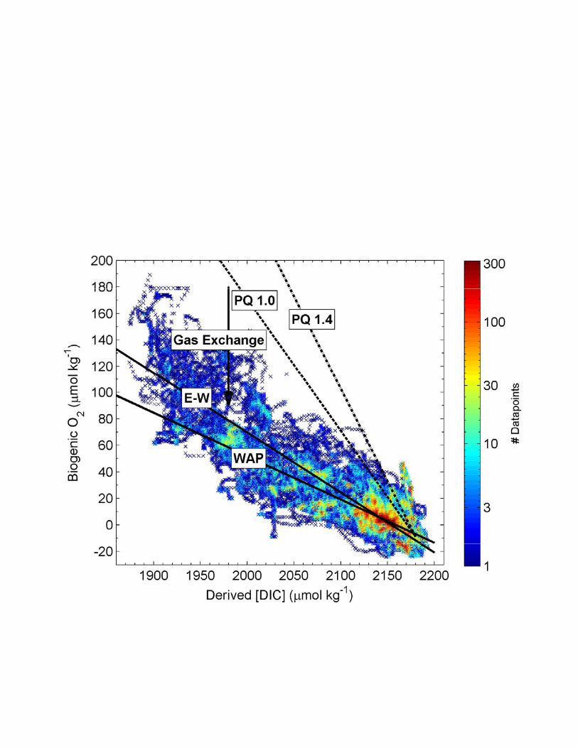
respectively). Figure 4 shows the corresponding relationship between O2 and total dissolved 484

inorganic carbon (DIC) concentrations derived from pCO2 and O2 /Ar data. For both the WAP 485

and E-W regions, the slope of the O2 : DIC relationship was significantly lower than the 486

expected photosynthetic stoichiometry (photosynthetic quotient, PQ, 1.0 - 1.4 mol O2 : mol DIC; 487

[Laws, 1991]). This discrepancy can be explained by the differential rate of sea-air O2 and CO2 488

exchange. Faster air-sea equilibration of O2 results in a shorter residence time of this gas in the 489

mixed layer, and a more rapid ventilation of photosynthetically-derived O2. During our cruise, 490

the average residence time of O2 in the mixed layer was < 1 week, given the mean wind speed 491

(9.2 m s-1) and MLD (26 m) observed across the survey region. In contrast, disequilibria in 492

pCO2, which is buffered by the seawater carbonate system, can persist for many weeks and even 493

months in the surface mixed layer [Takahashi et al., 2009]. The degree of uncoupling between 494

CO2 and O2 in the mixed layer should thus provide insight into temporal evolution of biological 495

productivity in surface waters. Regions where the biological production signal is ‘older’ should 496

exhibit a higher degree of CO2 – O2 uncoupling. In our data set, the lower O2-DIC slope in the 497

WAP region (0.33 vs. 0.45 for the E-W transect; Fig. 4) suggests that the production signal was 498

integrated over a longer time interval. Indeed, remote sensing data show the presence of 499

phytoplankton blooms in the WAP for over two months prior to our sampling (see Fig. 8b and 500

section 3.6). In contrast, much of the biological production along the E-W region occurred 501

following recent ice retreat, with shorter time interval for gas exchange to uncouple O2 and DIC. 502

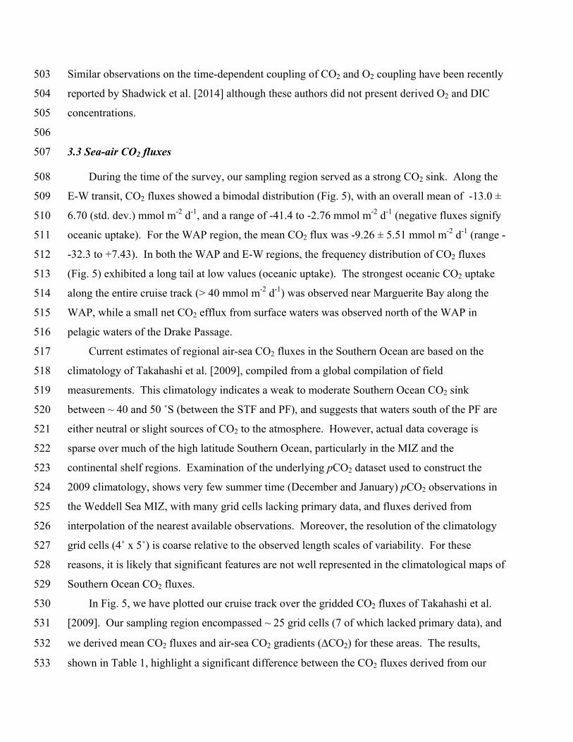
Similar observations on the time-dependent coupling of CO2 and O2 coupling have been recently 503

reported by Shadwick et al. [2014] although these authors did not present derived O2 and DIC 504

concentrations. 505

506

3.3 Sea-air CO2 fluxes 507

During the time of the survey, our sampling region served as a strong CO2 sink. Along the 508

E-W transit, CO2 fluxes showed a bimodal distribution (Fig. 5), with an overall mean of -13.0 ± 509

6.70 (std. dev.) mmol m-2 d-1, and a range of -41.4 to -2.76 mmol m-2 d-1 (negative fluxes signify 510

oceanic uptake). For the WAP region, the mean CO2 flux was -9.26 ± 5.51 mmol m-2 d-1 (range -511

-32.3 to +7.43). In both the WAP and E-W regions, the frequency distribution of CO2 fluxes 512

(Fig. 5) exhibited a long tail at low values (oceanic uptake). The strongest oceanic CO2 uptake 513

along the entire cruise track (> 40 mmol m-2 d-1) was observed near Marguerite Bay along the 514

WAP, while a small net CO2 efflux from surface waters was observed north of the WAP in 515

pelagic waters of the Drake Passage. 516

Current estimates of regional air-sea CO2 fluxes in the Southern Ocean are based on the 517

climatology of Takahashi et al. [2009], compiled from a global compilation of field 518

measurements. This climatology indicates a weak to moderate Southern Ocean CO2 sink 519

between ~ 40 and 50 ˚S (between the STF and PF), and suggests that waters south of the PF are 520

either neutral or slight sources of CO2 to the atmosphere. However, actual data coverage is 521

sparse over much of the high latitude Southern Ocean, particularly in the MIZ and the 522

continental shelf regions. Examination of the underlying pCO2 dataset used to construct the 523

2009 climatology, shows very few summer time (December and January) pCO2 observations in 524

the Weddell Sea MIZ, with many grid cells lacking primary data, and fluxes derived from 525

interpolation of the nearest available observations. Moreover, the resolution of the climatology 526

grid cells (4˚ x 5˚) is coarse relative to the observed length scales of variability. For these 527

reasons, it is likely that significant features are not well represented in the climatological maps of 528

Southern Ocean CO2 fluxes. 529

In Fig. 5, we have plotted our cruise track over the gridded CO2 fluxes of Takahashi et al. 530

[2009]. Our sampling region encompassed ~ 25 grid cells (7 of which lacked primary data), and 531

we derived mean CO2 fluxes and air-sea CO2 gradients (CO2) for these areas. The results, 532

shown in Table 1, highlight a significant difference between the CO2 fluxes derived from our 533

MIMS data, and those from the climatology. In December, the climatology shows our sampling 534

region to be near neutral with respect to air-sea CO2 fluxes (1.4 ± 0.90 mmol m-2 d-1), whereas 535

our measurements show mean oceanic uptake of 10 (± 5.8) mmol m-2 d-1. In January, the 536

climatological CO2 flux is -2.4 ± 0.92 mmol m-2 d-1, compared to -9.9 ± 4.2 mmol m-2 d-1 derived 537

from our measurements. The climatology represents a mean value derived from many years of 538

observations, and some inter-annual variability is expected. During our survey, we measured 539

significantly higher air-sea CO2 disequilibria than are present in the climatology; for December 540

and January, respectively, we observed an average CO2 of -91 and -108 atm, compared to the 541

climatological values of ~ +17 and -39 atm. These differences are likely too large to represent 542

simple inter-annual variability, and likely reflect real differences in the underlying distribution of 543

data. Our results thus suggest significantly higher oceanic CO2 uptake in high latitude Antarctic 544

waters than is represented by the global climatology. Similar observations have been reported in 545

previous studies [Arrigo et al., 2008; Bellerby et al., 2004; Hoppema et al., 2000a]. Note that the 546

apparent difference in sea-air CO2 fluxes between our observations and the climatology is ~ 2-547

fold larger if we compute the fluxes using ship-based winds as opposed to the weekly averaged 548

NCEP reanalysis product. 549

High latitude Antarctic waters, and the MIZ in particular, should be effective at sequestering 550

CO2 from the atmosphere due to the coupling of biological productivity with sea ice dynamics. 551

As observed in our study and that of previous authors [Bakker et al., 2008; Jones et al., 2010], 552

ice retreat leads to enhanced phytoplankton biomass and strong CO2 uptake. Previous studies 553

have shown that much of the CO2 taken up by spring phytoplankton growth can effectively be 554

sequestered into sub-surface layers during late summer cooling and the return of ice cover at the 555

end of the growing season [Sweeney, 2003]. Late season sea ice cover acts to limit outgassing of 556

high CO2 during the net heterotrophic period of the annual growing season, enhancing the CO2 557

sequestration efficiency of surface waters. For this reason, Antarctic continental shelf waters are 558

likely to contribute disproportionately to Southern Ocean CO2 uptake [Arrigo et al., 2008]. 559

Inclusion of more data from these regions into updated climatologies (with finer-scale grid cell 560

resolution, and greater seasonal data coverage) could lead to revised estimates of Southern Ocean 561

CO2 uptake, with significant implications for the global C budget. 562

563

3.4 N2 distribution 564

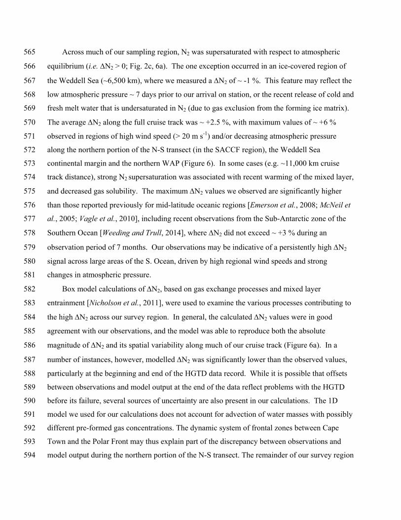
Across much of our sampling region, N2 was supersaturated with respect to atmospheric 565

equilibrium (i.e. N2 > 0; Fig. 2c, 6a). The one exception occurred in an ice-covered region of 566

the Weddell Sea (~6,500 km), where we measured a N2 of ~ -1 %. This feature may reflect the 567

low atmospheric pressure ~ 7 days prior to our arrival on station, or the recent release of cold and 568

fresh melt water that is undersaturated in N2 (due to gas exclusion from the forming ice matrix). 569

The average N2 along the full cruise track was ~ +2.5 %, with maximum values of ~ +6 % 570

observed in regions of high wind speed (> 20 m s-1) and/or decreasing atmospheric pressure 571

along the northern portion of the N-S transect (in the SACCF region), the Weddell Sea 572

continental margin and the northern WAP (Figure 6). In some cases (e.g. ~11,000 km cruise 573

track distance), strong N2 supersaturation was associated with recent warming of the mixed layer, 574

and decreased gas solubility. The maximum N2 values we observed are significantly higher 575

than those reported previously for mid-latitude oceanic regions [Emerson et al., 2008; McNeil et 576

al., 2005; Vagle et al., 2010], including recent observations from the Sub-Antarctic zone of the 577

Southern Ocean [Weeding and Trull, 2014], where N2 did not exceed ~ +3 % during an 578

observation period of 7 months. Our observations may be indicative of a persistently high N2 579

signal across large areas of the S. Ocean, driven by high regional wind speeds and strong 580

changes in atmospheric pressure. 581

Box model calculations of N2, based on gas exchange processes and mixed layer 582

entrainment [Nicholson et al., 2011], were used to examine the various processes contributing to 583

the high N2 across our survey region. In general, the calculated N2 values were in good 584

agreement with our observations, and the model was able to reproduce both the absolute 585

magnitude of N2 and its spatial variability along much of our cruise track (Figure 6a). In a 586

number of instances, however, modelled N2 was significantly lower than the observed values, 587

particularly at the beginning and end of the HGTD data record. While it is possible that offsets 588

between observations and model output at the end of the data reflect problems with the HGTD 589

before its failure, several sources of uncertainty are also present in our calculations. The 1D 590

model we used for our calculations does not account for advection of water masses with possibly 591

different pre-formed gas concentrations. The dynamic system of frontal zones between Cape 592

Town and the Polar Front may thus explain part of the discrepancy between observations and 593

model output during the northern portion of the N-S transect. The remainder of our survey region 594

is less prone to advection, owing to a (zonally) more homogeneous water mass structure. In the 595

MIZ, uncertainty in the model calculations may result from sea-ice dependent processes. The 596

sea ice history used in the model was derived from reprocessed satellite data with a relatively 597

coarse spatial resolution. Sea ice cover exerts a significant influence on the strength of air-sea 598

exchange, and errors in the representation of sea ice cover or in the parameterization of ice 599

effects on gas exchange coefficients [Loose et al., 2009] would lead to uncertainty in the N2 600

calculation. Notwithstanding these sources of uncertainty, we conclude that our observations 601

provide a reasonable validation of the Nicholson et al. [2011] model in various Southern Ocean 602

regions with high wind speeds and strong temporal changes in atmospheric pressure. Additional 603

GTD data and higher resolution physical models will be needed to further examine the 604

distribution of N2 across various Southern Ocean regions. Inclusion of GTD sensors on new 605

biogeochemical ocean floats and gliders [Emerson et al., 2002; Nicholson et al., 2008] will be 606

particularly useful in this respect. 607

608

3.5 Physical vs. biological controls on O2 saturation states 609

Unlike N2, oxygen saturation states are strongly influenced by both physical and biological 610

processes. We quantified the physical effects on O2 saturation state (O2phys), using 611

simultaneous MIMS and optode measurements (see methods). Measured values of O2phys (i.e. 612

optode O2 – MIMS O2 /Ar) showed significant variability along our cruise track (Fig. 7a), 613

with values ranging from ~ -5% (undersaturation) to > +10% (supersaturation). This range of 614

values is significantly larger than that reported recently by Shadwick et al. [2014], who measured 615

± 3% O2phys along a transect from Australia to the Antarctic MIZ. In our study, maximum O2 616

supersaturation was observed in the WAP region (~ 11,000 km cruise track), whereas 617

undersaturation was largely confined to several regions of local sea-ice cover (Fig. 7a). Box 618

model calculations of O2pe (i.e. the entrainment of non-biologically modified sub-surface 619

waters) showed reasonably good agreement with observations, and were able to reproduce the 620

spatial pattern of O2phys along much of the cruise track (Fig. 7a). There were, however, notable 621

offsets between the modelled and observed values in some areas, with the model tending to 622

under-predict the observations, as seen for N2 (Fig. 6). The largest discrepancies between the 623

model and observations occurred along the N-S transect, and in the WAP region. As discussed 624

above for N2, the discrepancy between modelled and observed O2 along the N-S transect may 625

have resulted from the lateral advection of heterogeneous waters masses. By comparison, the 626

high apparent values of O2phys measured in the WAP (in excess of +10%) are more difficult to 627

reconcile with known physical processes driving O2 supersaturation in the mixed layer. Given 628

the extremely high O2 concentrations in this region (> 60% O2 supersaturation), the optode was 629

measuring at the outer limit of its calibration range, and we cannot exclude measurement errors 630

leading to an overestimation of O2phys. Moreover, the shallow mixed layers and bottom depths 631

in the coastal WAP make this region susceptible to physically induced O2 super-saturation 632

resulting from bubble injection under high wind speeds. Under these conditions, our 633

calculations, which assume 100% O2 saturation in sub-surface waters, would underestimate 634

O2pe. 635

In addition to our calculations of O2pe, we used the box model to derive an O2 entrainment 636

term associated with the transport of biologically-modified waters into the mixed layer. This 637

entrainment term, O2be, can be used to correct O2/Ar-derived NCP estimates, neglecting the 638

contribution of purely physical entrainment processes (O2pe) that have no significant effect on 639

O2 /Ar. The distribution of modelled O2be along the cruise track is shown in Fig. 7b, along 640

with our O2 /Ar observations. For much of our survey region, the magnitude of the 641

biologically-modified entrainment flux was small compared to the mixed layer O2 /Ar signal. 642

There were, however, a number of areas (particularly along the N-S transect), where the two O2 643

fluxes were similar in magnitude. The variability in modelled O2be results from differences in 644

O2 depth profiles and mixed layer depth history along the cruise track. Under conditions where 645

sub-surface O2 is lower than mixed layer values, due to net heterotrophy in the sub-euphotic 646

zone, entrainment of biologically-modified sub-surface waters acts to decrease the O2 saturation 647

in the mixed layer (i.e. O2be < 0). This phenomenon was clearly observed in the ice-covered 648

waters of the N-S and E-W transects (Fig. 7b) where O2be showed a clear negative signature. In 649

contrast, we observed a number of regions, mostly in the WAP, where O2be was positive, 650

reflecting the entrainment of a remnant productivity signal prior to mixed layer shoaling. 651

Jonsson et al. [2013] have also noted the importance of entrainment as a potential source of O2 652

into the mixed layer. Quantification of this O2 source depends on an understanding of mixed 653

layer depth history and the choice of an appropriate sub-surface O2 end-member (cO2,sub). Based 654

on an analysis of the mixed layer time-series produced by the PSY3V3 model output, we chose a 655

subsurface O2 end-member (cO2,sub) 20 - 25 m below the mixed layer. We note, however, that 656

these end-member O2 values, and the corresponding mixed layer histories are subject to 657

potentially significant uncertainty. Nonetheless, as discussed below, we found that the derived 658

O2be term was able to produce entrainment-corrected O2 /Ar-NCP values that showed good 659

agreement with independent estimates based on DIC deficit calculations. It is also important to 660

note that the entrainment term was generally small compared to the biological O2 production 661

signal (i.e. O2/Ar) in the mixed layer for much of our survey region. 662

663

3.6 Net Community Production 664

In recent years, a number of studies have examined Southern Ocean NCP using mixed layer 665

O2 /Ar measurements, both from discrete samples and continuous underway analysis. This 666

work has been largely based on the approach developed by Kaiser et al. [2005] and Reuer et al. 667

[2007], where the mixed layer O2 budget is assumed to be in a steady-state, with negligible 668

vertical or lateral fluxes. Under these conditions, the biologically-induced flux of O2 to the 669

atmosphere (O2-bioflux, as defined by Eq. 11) provides a measure of NCP. The assumptions 670

used in these calculations are problematic in weakly stratified and highly dynamic waters 671

encountered over large portions of the Southern Ocean. Jonsson et al. [2013] have shown that 672

O2-bioflux provides good regional estimates of Southern Ocean NCP (± ~ 25%), but significant 673

offsets can exist at smaller scales due to a temporal decoupling between O2 production and air-674

sea exchange, and to vertical O2 fluxes across the base of the mixed layer. Using our box model 675

results (section 3.5), we were able to estimate the contribution of entrainment fluxes to the 676

surface biological O2 budget, and we used this information to correct NCP estimates derived 677

from surface O2/Ar data. However, our calculations do not include other physical processes 678

such as upwelling and diapycnal mixing that can also influence NCP derived from O2/Ar 679

measurements [Jonsson et al., 2013]. 680

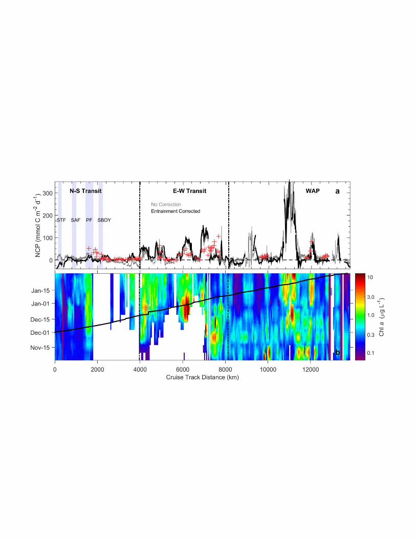
Figure 8 presents NCP estimates along our cruise track derived from O2/Ar, with and 681

without a correction for biologically-modified entrainment fluxes (O2be). The figure also shows 682

satellite-derived Chla observations, which provide information on the temporal evolution of 683

phytoplankton biomass prior to our sampling. Across the full survey region, O2 /Ar-derived 684

NCP ranged from ~ -40 to > 300 mmol O2 m-2 d-1. The lowest NCP values were found along the 685

N-S transect (maximum ~ 20 mmol O2 m-2 d-1). Despite the low overall productivity observed 686

along much of this transect, there were localized regions of elevated NCP associated with 687

regional frontal features - most notably in the vicinity of the Polar Front zone where vertical 688

mixing can supply Fe to iron-limited surface waters [Debaar et al., 1995]. Without a correction 689

for entrainment, waters of the Weddell Sea MIZ (both along the N-S and E-W transects) 690

appeared to be net heterotrophic (i.e. NCP <0). However, this apparent net heterotrophic 691

signature was eliminated after accounting for the entrainment fluxes (O2be). In contrast, the 692

entrainment-corrected NCP remained below zero in the STF zone, and in several other localized 693

regions along the cruise track. Net heterotrophy in the STF zone seems unlikely, given the 694

enhanced Chla concentrations in this region (Fig. 3c). Rather, we suggest that an overestimation 695

of the O2 entrainment term (O2be), resulting from errors in the selection of a sub-MLD end-696

member or in the derived mixed layer depth history, is a more likely explanation for this feature. 697

Regions of net heterotrophy observed along other portions of our cruise track (e.g. between 8000 698

- 9000 km) were largely confined to waters with very low (< 0.3 g L-1) Chla concentrations. In 699

contrast, the most productive waters, with NCP in excess of 300 mmol O2 m-2 d-1 were observed 700

in the central WAP region, where high phytoplankton biomass was detected for over two months 701

prior to our sampling. In these high NCP waters, the entrainment correction term was generally 702

small compared to the biological production term. 703

The variability of our O2/Ar-derived NCP values is somewhat higher than previous 704

observations for the Southern Ocean, but the mean values for each of survey regions are within 705

the range of recently published estimates. Excluding the negative NCP values in the STF zone, 706

the average NCP for the N-S, E-W and WAP transects was 9.3, 31 and 14 mmol O2 m-2 d-1, 707

respectively. The low mean NCP value for the WAP region seems initially surprising, given the 708

extremely elevated NCP observed at ~ 11,000 km along the cruise track. Outside of this one 709

productivity hot-spot, however, much of the WAP region had relatively low (and in some cases 710

even negative) NCP. Excluding the negative values, the mean NCP value in the WAP is 48 711

mmol O2 m-2 d-1. By comparison, exclusion of negative NCP values from the E-W transect only 712

increased the mean NCP by ~ 10%. These results suggest that localized net heterotrophy was 713

more significant to regional NCP budgets in the WAP region. 714

Based on discrete sampling of surface O2/Ar, Reuer et al. [2007] reported mean NCP 715

estimates ranging from 20 – 36 mmol O2 m-2 d-1 for the Subantarctic Zone, Polar Frontal Zone 716

and Antarctic Zone. More recently, Shadwick et al. [2014] have reported a range of NCP 717

estimates from 15 – 75 mmol O2 m-2 d-1 (assuming a photosynthetic quotient of 1.4) along a 718

transect from Australia to the Antarctic continent, while Cassar et al. [2011] report NCP of ~ up 719

to 150 mmol O2 m-2 d-1 for sub-Antarctic waters south of Australia. The maximum NCP values 720

measured along our cruise track (> 300 mmol O2 m-2 d-1) are among the highest reported for the 721

Southern Ocean, yet these values are not without precedent. Recent time-series work at the 722

Palmer Station LTER site along the WAP [Tortell et al., 2014], show maximum NCP values 723

similar to the highest values we observed along the WAP region of our cruise track. 724

Independent NCP estimates, based on calculated seasonal DIC deficits at discrete sampling 725

stations, showed good general coherence with our O2 /Ar-derived values. Both the spatial 726

distribution and range of NCP values were similar for the two methods. The agreement between 727

the two estimates was particularly good in the WAP region (unfortunately, DIC samples were 728

not collected in the vicinity of Marguerite Bay, where the highest NCP values were observed), 729

and also south of the SBdy frontal zone along the N-S transect. In contrast, there were apparent 730

offsets between the two NCP estimates in the vicinity of the PF and in the highest productivity 731

regions of the E-W transit. In addition to the uncertainties discussed above for O2 /Ar-derived 732

NCP, NCP estimates from DIC deficits are also subject to potential errors. The most significant 733

source of uncertainty in these calculations relates to the time-period over which DIC uptake is 734

normalized. In our analysis, we assumed that DIC deficits began to accumulate following the 735

initiation of the spring phytoplankton blooms (as judged by satellite-based chlorophyll 736

measurements; Fig. S3). This approach does not account for potential productivity under sea-ice 737

[Arrigo et al., 2012], which is not visible by remote sensing. Although our approach is, by 738

necessity, somewhat simplistic, we are encouraged by the good correspondence of DIC and 739

O2/Ar-derived estimates of surface water productivity. Our results suggest that mixed layer 740

O2 /Ar measurements have the capacity to provide meaningful NCP estimates with high spatial 741

resolution. 742

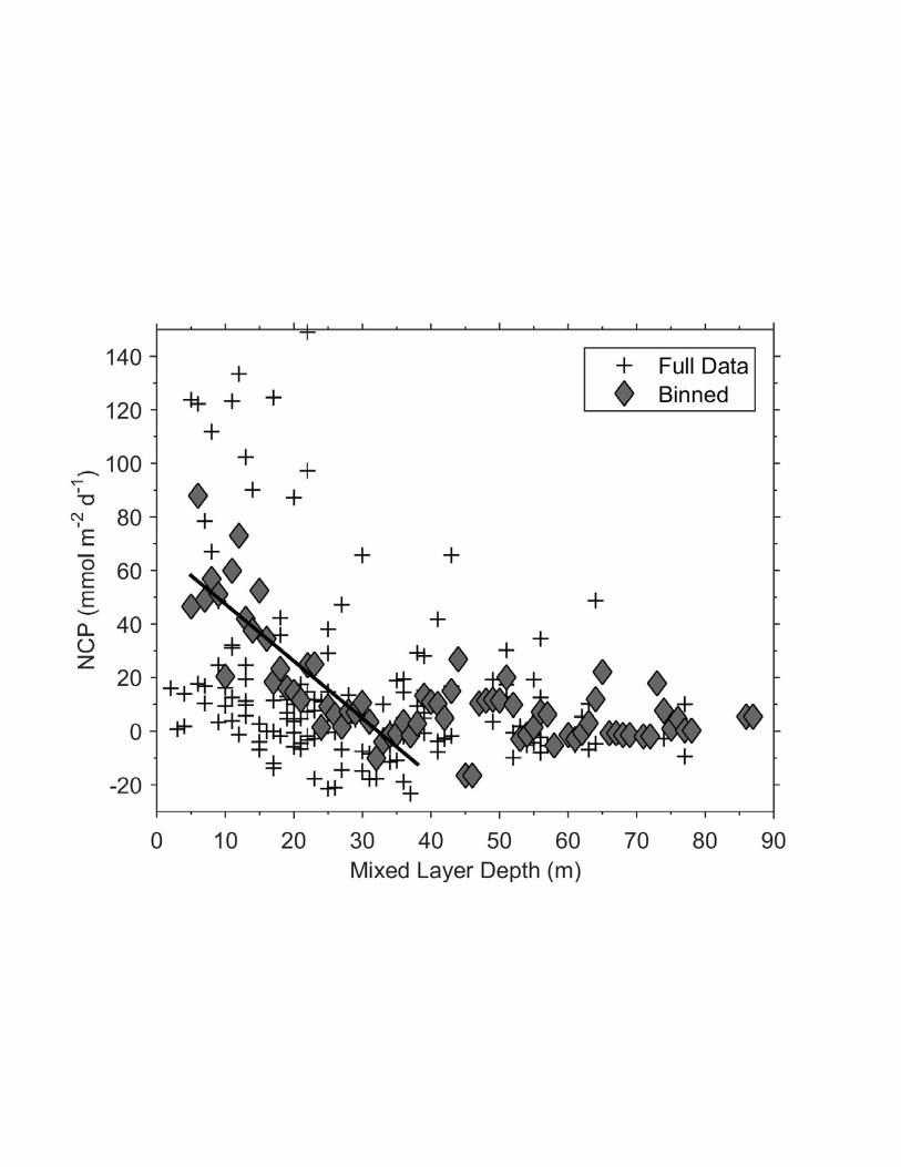
Beyond the absolute value of our derived NCP estimates, the spatial distribution of 743

biological productivity across our survey region is of interest. Since macro-nutrients were 744

plentiful across our entire survey region (minimum NO3- > 8 M), light and/or iron availability 745

are the most likely bottom-up controls on phytoplankton productivity. Although no iron data are 746

available for our cruise, we assume, based on previous studies, that Fe availability was highest in 747

regions of sea ice melt along the continental shelf [Gerringa et al., 2012; Klunder et al., 2011], 748

where high NCP was observed. To examine the influence of light availability on surface water 749

productivity, we derived NCP estimates for the regions surrounding each of our hydrographic 750

stations (within 5 km), and correlated these values to the mixed layer depths obtained from CTD 751

data. As shown in Fig. 9, we observed a weak negative trend between NCP and MLD, 752

particularly for stations with mixed layer depths less than 40 m. Taking only stations with MLD 753

< 40 m, the correlation between MLD and NCP was statistically significant (for 1 m binned data, 754

r = -0.86, p < .001). This relationship provides some evidence for light-dependent productivity, 755

as suggested previously [Cassar et al., 2011; Huang et al., 2012; Shadwick et al., 2014]). We 756

note, however, that instantaneous MLD estimates do not necessarily provide a good indication of 757

light availability over time scales relevant to our NCP calculations. A more refined analysis 758

could be used, taking into account the time-dependent history of MLD, surface irradiance and 759

water column light extinction (based on Chla concentrations). Even without this added 760

complexity, our derived NCP estimates likely reflect the dominant influence of light, nutrient 761

supply and sea ice cover on biological productivity across strongly distinct regions of the 762

Southern Ocean. 763

764

4. Conclusions and Future Directions 765

766

Our results provide new information on the distribution of pCO2, O2, and N2 in contrasting 767

Southern Ocean regions, and insight into the underlying factors driving these distributions. 768

Across our survey region, strong hydrographic variability led to large gradients in phytoplankton 769

biomass, which, in turn, exerted a significant influence on surface water pCO2 and O2/Ar 770

distributions. This biological signature was modified by physical processes including sea-air 771

exchange, and mixed layer entrainment. Using our observations and box model calculations, we 772

were able to quantify the physical contributions to surface water O2 and N2 disequilibria, and we 773

used this information to refine our estimates of NCP from surface O2/Ar observations. The 774

NCP rates derived in this manner were consistent with independent measurements based on 775

surface DIC deficits, providing a high spatial resolution description of biological productivity 776

across the cruise track. Our surface water pCO2 observations suggest that the high latitude 777

Southern Ocean may be a stronger sink for atmospheric CO2 than is currently represented in the 778

global climatology [Takahashi et al., 2009]. To the extent that our results are applicable on a 779

broad regional scale, there may thus be a need to critically re-evaluate current estimates of 780

Southern Ocean CO2 uptake. 781

The increasing availability of autonomous ship-board instruments for surface gas measurements 782

(e.g. optodes, GTDs and sea-going mass spectrometers) has significantly expanded the spatial 783

and temporal coverage of oceanic dissolved gas observations. In the future, continued 784

deployments of these autonomous instruments, along with instrumented floats, gliders and 785

moorings [Emerson et al., 2008; Nicholson et al., 2008], will allow us to assemble a more robust 786

database of Southern Ocean N2, O2, O2 /Ar to help constrain NCP and air-sea exchange 787

processes. Moreover, additional pCO2 measurements in poorly sampled regions will help to 788

refine mean climatological CO2 fluxes for the Southern Ocean. In conjunction with increased 789

data coverage, more sophisticated modelling approaches could be used to interpret surface gas 790

distributions, taking into account smaller-scale physical processes that act to perturb the mixed 791

layer mass balance. Improved datasets and models will facilitate more robust NCP and CO2 flux 792

estimates, and increase our understanding of the Southern Ocean’s role in global biogeochemical 793

cycles. 794

795

5. Acknowledgements 796

797

Data are freely available upon request from the corresponding author (ptortell@eos.ubc.ca). 798

Support for this work was provided from the Natural Sciences and Engineering Council of 799

Canada (P. Tortell), the Von Humboldt Foundation (P. Tortell), the UBC Peter Wall Institute for 800

Advanced Studies (P. Tortell), the OCEANET project of the WGL Leibniz Association (A. 801

Körtzinger), the German Science Foundation’s O2-Floats project (grant KO 1717/3-1; H. Bittig), 802

and from the EU project CARBOCHANGE (grant no. 264879; M. Hoppema). We acknowledge 803

the tremendous leadership of the late Eberhard Fahrbach (AWI) as chief scientist for our cruise, 804

and the efforts of Gerd Rohardt (AWI) in the compilation and quality control of all hydrographic 805

data. Christopher Payne and Constance Couture (UBC) provided ship-board technical assistance 806

with the mass spectrometer. 807

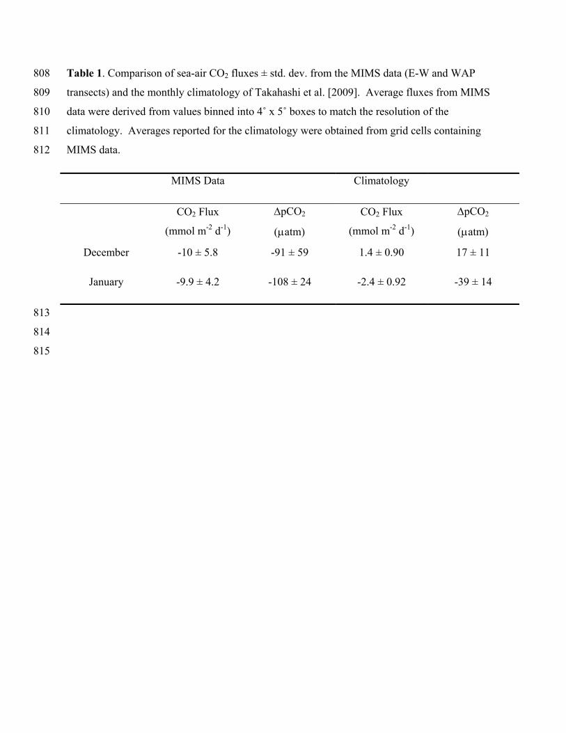
Table 1. Comparison of sea-air CO2 fluxes ± std. dev. from the MIMS data (E-W and WAP 808

transects) and the monthly climatology of Takahashi et al. [2009]. Average fluxes from MIMS 809

data were derived from values binned into 4˚ x 5˚ boxes to match the resolution of the 810

climatology. Averages reported for the climatology were obtained from grid cells containing 811

MIMS data. 812

MIMS Data Climatology

CO2 Flux

(mmol m-2 d-1)

pCO2

atm)

CO2 Flux

(mmol m-2 d-1)

pCO2

atm)

December -10 ± 5.8 -91 ± 59 1.4 ± 0.90 17 ± 11

January -9.9 ± 4.2 -108 ± 24 -2.4 ± 0.92 -39 ± 14

813

814

815

Figure Legends 816

817

Figure 1. Map of the sampling area showing the cruise track (solid red line) and the 818

position of various hydrographic fronts (dotted lines). From north to south, the fronts are: 819

Subtropical Front (STF), Sub-Antarctic Front (SAF), Polar Front (PF), Southern Antarctic 820

Circumpolar Current Front (SACCF) and Southern Boundary of the Antarctic Circumpolar 821

Current (SBdy). The location of mean frontal positions was derived from Orsi et al. [1995]. N-822

S, E-W and WAP denote different portions of our sampling region, as described in the text. 823

Grey / black shading around the Antarctic continent represents the mean sea ice cover during the 824

period of our survey, derived from the AMSR-E satellite product. 825

826

Figure 2. Spatial distribution of sea-surface temperature, SST (a), salinity (b), N2 827

saturation, N2 (c), Chla fluorescence (d), pCO2 (e), and biological O2 saturation, O2 /Ar (f) 828

along the cruise track. Inset figures show a detailed view of the property distributions along the 829

WAP transect. Note that pCO2 and N2 data are not available for the full cruise track due to 830

instrument problems. 831

832

Figure 3. Distribution of pCO2 (a), biological O2 saturation, O2 /Ar (b), Chla 833

fluorescence (c) and sea surface temperature (d) along the cruise track. Black vertical lines show 834

the demarcation between the different portions of the cruise track, vertical grey shaded bars show 835

regions with more than 50% ice cover and blue shaded areas with dotted lines show the position 836

of different frontal regions. 837

838

Figure 4. Relationship between dissolved inorganic carbon (DIC) concentrations and 839

biogenic O2. DIC values were obtained from MIMS pCO2 data, using empirically-derived 840

alkalinity values (based on surface salinity). Biogenic O2 (i.e. the amount of excess O2 in the 841

mixed layer derived from biological production) was computed from O2/Ar data using a 842

temperature and salinity-dependent O2 solubility function. Solid lines show the DIC-O2 843

relationship for the E-W and WAP portions of the ship track derived from a Type II regression 844

analysis, while dashed lines show the expected DIC-O2 relationship for a photosynthetic quotient 845

(PQ) of 1 or 1.4 mol O2 produced per mol DIC consumed. The slope of the O2-DIC relationship 846

is 0.45 and 0.33 for the E-W and WAP regions, respectively. 847

848

Figure 5. Frequency distribution of air-sea CO2 fluxes along the E-W and WAP regions 849

of the cruise track (a). Panels (b) and (c) show the ship-track plotted over the monthly 850

climatological CO2 flux derived from the global climatology of Takahashi et al. [2009]. 851

Negative fluxes imply oceanic uptake of CO2. 852

853

Figure 6. Nitrogen saturation, N2 (a), atmospheric pressure history (b) and wind speed 854

history (c) along the cruise track. The black line in panel (a) shows the N2 value derived from 855

GTD measurements, while the red line shows the results of box model calculations (see text for a 856

full description). Grey vertical patches in panel (a) show regions with greater than 50% ice 857

cover. Atmospheric pressure and wind speed data shown in panels (b) and (c) were derived from 858

NCEP re-analysis. The y axis in panels (b) and (c) represents the number of days prior to the 859

ship’s arrival at a location along the cruise track. 860

861

Figure 7. Effects of physical and biological processes on mixed layer O2 saturation state. 862

The black line in panel (a) shows observed values of O2phys, derived from MIMS O2/Ar and 863

optode O2, while the red line shows the results of box model calculations, including physical 864

terms in the O2 budget (i.e. air-sea processes and entrainment of non-biologically modified sub-865

surface waters, O2pe). Panel (b) shows biological effects on the surface O2 budget resulting 866

from in situ NCP (as reflected by surface O2/Ar measurements) and modelled entrainment of 867

biologically-modified sub-surface waters (O2be). Panel (c) shows O2 depth profiles along the 868

cruise track derived from CTD observations. The thin black line and crosses represent the 869

computed mixed layer depth, while the thicker line represents a 5 point running mean. 870

871

Figure 8. Distribution of net community production (NCP) along the cruise track (a), and 872

the time-history of Chla concentrations derived from the Aqua-Modis remote sensing product 873

(b). Black and grey lines in (a) represent NCP estimates derived from O2/Ar data, with and 874

without a correction for biologically-modified O2 entrainment fluxes (O2be). The red crosses in 875

(a) represent NCP estimated from seasonal DIC deficits in the mixed layer. Vertical blue patches 876

in (a) show frontal regions. The black line in (b) shows the location of the research vessel, while 877

white patches denote sea-ice cover. Note the logarithmic scaling of the Chla axis. 878

879

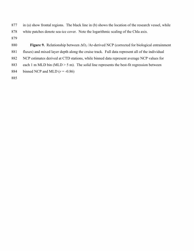
Figure 9. Relationship between O2 /Ar-derived NCP (corrected for biological entrainment 880

fluxes) and mixed layer depth along the cruise track. Full data represent all of the individual 881

NCP estimates derived at CTD stations, while binned data represent average NCP values for 882

each 1 m MLD bin (MLD > 5 m). The solid line represents the best-fit regression between 883

binned NCP and MLD (r = -0.86) 884

885

References 886

887

Arrigo, K. R., and G. L. van Dijken (2003), Phytoplankton dynamics within 37 Antarctic coastal 888

polynya systems, Journal of Geophysical Research-Oceans, 108(C8). 889

Arrigo, K. R., and G. L. van Dijken (2004), Annual changes in sea-ice, chlorophyll a, and 890

primary production in the Ross Sea, Antarctica, Deep-Sea Research Part II, 51(1-3), 117-891

138. 892

Arrigo, K. R., G. van Dijken, and M. Long (2008), Coastal Southern Ocean: A strong 893

anthropogenic CO2 sink, Geophysical Research Letters, 35(21). doi L21602 894

10.1029/2008gl035624 895

Arrigo, K. R., D. K. Perovich, R. S. Pickart, Z. W. Brown, G. L. van Dijken, K. E. Lowry, M. M. 896

Mills, M. A. Palmer, W. M. Balch, and F. Bahr (2012), Massive phytoplankton blooms 897

under Arctic sea ice, Science, 336(6087), 1408-1408. 898

Bakker, D. C. E., M. Hoppema, M. Schroder, W. Geibert, and H. J. W. De Baar (2008), A rapid 899

transition from ice covered CO2-rich waters to a biologically mediated CO2 sink in the 900

eastern Weddell Gyre, Biogeosciences, 5(5), 1373-1386. 901

Bellerby, R. G. J., M. Hoppema, E. Fahrbach, H. J. W. de Baar, and M. H. C. Stoll (2004), 902

Interannual controls on Weddell Sea surface water fCO2 during the autumn-winter 903

transition phase, Deep Sea Research Part I: Oceanographic Research Papers, 51(6), 793-904

808. 905

Boyd, P. W. (2002), Environmental factors controlling phytoplankton processes in the Southern 906

Ocean, Journal of Phycology, 38(5), 844-861. 907

Brewer, P. G., A. L. Bradshaw, and R. T. Williams (1986), Measurements of total carbon 908

dioxide and alkalinity in the North Atlantic Ocean in 1981, in The Changing Carbon Cycle, 909

edited, pp. 348-370, Springer. 910

Caldeira, K., and P. B. Duffy (2000), The role of the Southern Ocean in uptake and storage of 911

anthropogenic carbon dioxide, Science, 287(5453), 620-622. 912

Carrillo, C. J., R. C. Smith, and D. M. Karl (2004), Processes regulating oxygen and carbon 913

dioxide in surface waters west of the Antarctic Peninsula, Marine Chemistry, 84(3-4), 161-914

179. 915

916

Cassar, N., M. L. Bender, B. A. Barnett, S. Fan, W. J. Moxim, H. Levy, and B. Tilbrook (2007), 917

The Southern Ocean biological response to Aeolian iron deposition, Science, 317(5841), 918

1067-1070. 919

Cassar, N., P. J. DiFiore, B. A. Barnett, M. L. Bender, A. R. Bowie, B. Tilbrook, K. Petrou, K. J. 920

Westwood, S. W. Wright, and D. Lefevre (2011), The influence of iron and light on net 921

community production in the Subantarctic and Polar Frontal Zones, Biogeosciences, 8(2), 922

227-237. 923

Castro-Morales, K., N. Cassar, D. R. Shoosmith, and J. Kaiser (2013), Biological production in 924

the Bellingshausen Sea from oxygen-to-argon ratios and oxygen triple isotopes, 925

Biogeosciences, 10(4), 2273-2291. 926

Coale, K. H., R. M. Gordon, and X. J. Wang (2005), The distribution and behavior of dissolved 927

and particulate iron and zinc in the Ross Sea and Antarctic circumpolar current along 170 928

degrees W, Deep-Sea Research Part I-Oceanographic Research Papers, 52(2), 295-318. 929

Craig, H., and T. Hayward (1987), Oxygen supersaturation in the ocean - biological versus 930

physical contributions, Science, 235(4785), 199-202. 931

Debaar, H. J. W., J. T. M. Dejong, D. C. E. Bakker, B. M. Loscher, C. Veth, U. Bathmann, and 932

V. Smetacek (1995), Importance of iron for phytoplankton blooms and carbon dioxide 933

drawdown in the Southern Ocean, Nature, 373(6513), 412-415. 934

Dickson, A. G., and F. J. Millero (1987), A comparison of the equilibrium constants for the 935

dissociation of carbonic acid in seawater media, Deep-Sea Research Part a-Oceanographic 936

Research Papers, 34(10), 1733-1743. 937

Dickson, A. G. (1994), Determination of dissolved oxygen in sea water by Winkler titration, 938

WHP Operations and Methods, 1-14. 939

Dickson, A. G., C. L. Sabine, and J. R. Christian (2007), Guide to best practices for ocean CO2 940

measurements. 941

Emerson, S., C. Stump, B. Johnson, and D. M. Karl (2002), In situ determination of oxygen and 942

nitrogen dynamics in the upper ocean, Deep Sea Research Part I: Oceanographic 943

Research Papers, 49(5), 941-952. 944

Emerson, S., C. Stump, and D. Nicholson (2008), Net biological oxygen production in the ocean: 945

Remote in situ measurements of O2 and N2 in surface waters, Global Biogeochemical 946

Cycles, 22(3). 947

Garcia, H. E., and L. I. Gordon (1992), Oyxygen solubility in seawater - better fitting equations, 948

Limnology and Oceanography, 37(6), 1307-1312. 949

Gerringa, L. J. A., A. C. Alderkamp, P. Laan, C. E. Thuroczy, H. J. W. De Baar, M. M. Mills, G. 950

L. van Dijken, H. van Haren, and K. R. Arrigo (2012), Iron from melting glaciers fuels the 951

phytoplankton blooms in Amundsen Sea (Southern Ocean): Iron biogeochemistry, Deep 952

Sea Research Part II: Topical Studies in Oceanography. 953

Hamme, R. C., and S. R. Emerson (2004), The solubility of neon, nitrogen and argon in distilled 954

water and seawater, Deep-Sea Research Part I, 51(11), 1517-1528. 955

Hamme, R. C., and S. R. Emerson (2006), Constraining bubble dynamics and mixing with 956

dissolved gases: Implications for productivity measurements by oxygen mass balance, 957

Journal of Marine Research, 64(1), 73-95. 958

Honjo, S., S. J. Manganini, R. A. Krishfield, and R. Francois (2008), Particulate organic carbon 959

fluxes to the ocean interior and factors controlling the biological pump: A synthesis of 960

global sediment trap programs since 1983, Progress in Oceanography, 76(3), 217-285. 961

Hoppema, M., L. Goeyens, and E. Fahrbach (2000a), Intense nutrient removal in the remote area 962

off Larsen Ice Shelf (Weddell Sea), Polar Biology, 23(2), 85-94. 963

Hoppema, M., M. H. C. Stoll, and H. J. W. de Baar (2000b), CO2 in the Weddell Gyre and 964

Antarctic Circumpolar Current: austral autumn and early winter, Marine Chemistry, 72(2), 965

203-220. 966

Hoppema, M., R. Middag, H. J. W. de Baar, E. Fahrbach, E. M. van Weerlee, and H. Thomas 967

(2007), Whole season net community production in the Weddell Sea, Polar Biology, 31(1), 968

101-111. 969

Huang, K., H. Ducklow, M. Vernet, N. Cassar, and M. L. Bender (2012), Export production and 970

its regulating factors in the West Antarctica Peninsula region of the Southern Ocean, 971

Global Biogeochemical Cycles, 26, 13. 972

Jennings, J. C., L. I. Gordon, and D. M. Nelson (1984), Nutrient depletion indicates high primary 973

productivity in the Weddell Sea. 974

Johnson, K. M., J. M. Sieburth, P. J. L. Williams, and L. Brandstrom (1987), Coulometric Total 975

Carbon-Dioxide Analysis for Marine Studies - Automation and Calibration, Marine 976

Chemistry, 21(2), 117-133. 977

Jones, E. M., D. C. E. Bakker, H. J. Venables, M. J. Whitehouse, R. E. Korb, and A. J. Watson 978

(2010), Rapid changes in surface water carbonate chemistry during Antarctic sea ice melt, 979

Tellus B. 980

Jonsson, B. F., S. C. Doney, J. Dunne, and M. Bender (2013), Evaluation of the Southern Ocean 981

O2/Arâ € based NCP estimates in a model framework, Journal of Geophysical Research: 982

Biogeosciences, 118(2), 385-399. 983

Kaiser, J., M. K. Reuer, B. Barnett, and M. L. Bender (2005), Marine productivity estimates 984

from continuous O2/Ar ratio measurements by membrane inlet mass spectrometry, 985

Geophysical Research Letters, 32(19). 986

Keeling, R. F. (1993), On the role of large bubbles in air-sea gas exchange and supersaturation in 987

the ocean, Journal of Marine Research, 51(2), 237-271. 988

Klunder, M. B., P. Laan, R. Middag, H. J. W. De Baar, and J. C. Van Ooijen (2011), Dissolved 989

iron in the Southern Ocean (Atlantic sector), Deep Sea Research Part II: Topical Studies in 990

Oceanography, 58(25), 2678-2694. 991

Kortzinger, A., et al. (2008), Seasonal cycle of O2 and pCO2 in the central Labrador Sea: 992

Atmospheric, biological, and physical implications, Global Biogeochemical Cycles, 22(1). 993

doi. 10.1029/2007GB003029 994

Laubscher, R. K., R. Perissinotto, and C. D. McQuaid (1993), Phytoplankton production and 995

biomass at frontal zones in the atlantic sector of the Southern Ocean, Polar Biology, 13(7), 996

471-481. 997

Laws, E. A. (1991), Photosynthetic quotients, new production and net community production in 998

the open ocean, Deep-Sea Res, 38(1), 143-167. 999

Liang, J. H., C. Deutsch, J. C. McWilliams, B. Baschek, P. P. Sullivan, and D. Chiba (2013), 1000

Parameterizing bubble-mediated air-sea gas exchange and its effect on ocean ventilation, 1001

Global Biogeochemical Cycles, 27(3), 894-905. 1002

Loose, B., W. R. McGillis, P. Schlosser, D. Perovich, and T. Takahashi (2009), Effects of 1003

freezing, growth, and ice cover on gas transport processes in laboratory seawater 1004

experiments, Geophysical Research Letters, 36(5). 1005

Lorbacher, K., D. Dommernget, P.P. Niiler, Köhl A. (2006), Ocean mixed layer depth: A 1006

subsurface proxy of ocean-atmosphere variability, Journal of Geophysical Research: 1007

Oceans, 111(C7). 1008

Marinov, I., A. Gnanadesikan, J. R. Toggweiler, and J. L. Sarmiento (2006), The Southern 1009

Ocean biogeochemical divide, Nature, 441(7096), 964-967. 1010

Martinson, D. G., and D. C. McKee (2012), Transport of warm Upper Circumpolar Deep Water 1011

onto the western Antarctic Peninsula continental shelf, Ocean Sci., 8(4), 433. 1012

McNeil, C., D. Katz, R. Wanninkhof, and B. Johnson (2005), Continuous shipboard sampling of 1013

gas tension, oxygen and nitrogen, Deep Sea Research Part I: Oceanographic Research 1014

Papers, 52(9), 1767-1785. 1015

McNeil, C. L., B. D. Johnson, and D. M. Farmer (1995), In situ measurement of dissolved 1016

nitrogen and oxygen in the ocean, Deep Sea Research Part I: Oceanographic Research 1017

Papers, 42(5), 819-826. 1018

Mehrbach, C., Culberso.Ch, J. E. Hawley, and R.M. Pytkowic (1973), Measurement of apparent 1019

dissociation constants of carbonic acid in seawater at atmospheric pressure, Limnology and 1020

Oceanography, 18(6), 897-907. 1021

Nicholson, D., S. Emerson, and C. C. Eriksen (2008), Net community production in the deep 1022

euphotic zone of the subtropical North Pacific gyre from glider surveys, Limnology and 1023

Oceanography, 53(5), 2226. 1024

Nicholson, D., S. Emerson, and C. C. Eriksen (2011), An inverse approach to estimate bubble-1025

mediated air-sea gas flux from inert gas measurements, Proceedings on the 6th 1026

International Symposium on Gas Transfer at Water Surfaces, Kyoto University Press. 1027

Orsi, A. H., H., T. Whitworth Iii, and W. D. Nowlin Jr (1995), On the meridional extent and 1028

fronts of the Antarctic Circumpolar Current, Deep Sea Research Part I: Oceanographic 1029

Research Papers, 42(5), 641-673. 1030

Pierrot, D., E. Lewis, and D. W. R. Wallace (2006), MS Excel program developed for CO2 1031

system calculations, ORNL/CDIAC-105. Carbon Dioxide Information Analysis Center, 1032

Oak Ridge National Laboratory, US Department of Energy, Oak Ridge, Tennessee. 1033

Planquette, H., R. M. Sherrell, S. Stammerjohn, and M. P. Field (2013), Particulate iron delivery 1034

to the water column of the Amundsen Sea, Antarctica, Marine Chemistry, 153, 15-30. 1035

Reuer, M. K., R. M. Sherrell, S. Stammerjohn, and M. P. Field (2007), New estimates of 1036

Southern Ocean biological production rates from O2/Ar ratios and the triple isotope 1037

composition of O-2, Deep-Sea Research Part I-Oceanographic Research Papers, 54(6), 1038

951-974. 1039

Rohardt, G., E. Fahrbach, and A. Wisotzki. (2011), Physical oceanography during 1040

POLARSTERN cruise ANT-XXVII/2, Alfred Wegener Institute, Helmholtz Center for 1041

Polar andMarine Research., Pangaea. 1042

Rubin, S. I., T. Takahashi, D. W. Chipman, and J. G. Goddard (1998), Primary productivity and 1043

nutrient utilization ratios in the Pacific sector of the Southern Ocean based on seasonal 1044

changes in seawater chemistry, Deep Sea Research Part I: Oceanographic Research 1045

Papers, 45(8), 1211-1234. 1046

Sarmiento, J. L., and J. R. Toggweiler (1984), A new model for the role of the oceans in 1047

determining atmospheric PCO2, Nature, 308(5960), 621-624. 1048

Sarmiento, J. L., N. Gruber, M. A. Brzezinski, and J. P. Dunne (2004), High-latitude controls of 1049

thermocline nutrients and low latitude biological productivity, Nature, 427(6969), 56-60. 1050

Sarmiento, J. L., and N. Gruber (2006), Ocean Biogeochemical Dynamics, Princeton University 1051

Press. 1052

Schlitzer, R. (2002), Carbon export fluxes in the Southern Ocean: results from inverse modeling 1053

and comparison with satellite-based estimates, Deep-Sea Research Part Ii-Topical Studies 1054

in Oceanography, 49(9-10), 1623-1644. 1055

Schudlich, R., and S. Emerson (1996), Gas supersaturation in the surface ocean: The roles of 1056

heat flux, gas exchange, and bubbles, Deep Sea Research Part II: Topical Studies in 1057

Oceanography, 43(2), 569-589. 1058

Sedwick, P. N., and G. R. DiTullio (1997), Regulation of algal blooms in Antarctic shelf waters 1059

by the release of iron from melting sea ice, Geophysical Research Letters, 24(20), 2515-1060

2518. 1061

Shadwick, E. H., B. Tilbrook, N. Cassar, T. W. Trull, and S. R. Rintoul (2014), Summertime 1062

physical and biological controls on O2 and CO2 in the Australian Sector of the Southern 1063

Ocean, Journal of Marine Systems. 1064

Smith, W. O., and D. M. Nelson (1985), Phytoplankton bloom produced by a receding ice edge 1065

in the Ross Sea - spatial coherence with the density field., Science, 227(4683), 163-166. 1066

Smith, W. O., and L. I. Gordon (1997), Hyperproductivity of the Ross Sea(Antarctica) polynya 1067

during austral spring, Geophy. Res. Lett., 24(3), 233-236. 1068

Sokolov, S., and S. R. Rintoul (2007), On the relationship between fronts of the Antarctic 1069

Circumpolar Current and surface chlorophyll concentrations in the Southern Ocean, 1070

Journal of Geophysical Research-Oceans, 112(C7). 1071

Sokolov, S. (2008), Chlorophyll blooms in the Antarctic Zone south of Australia and New 1072

Zealand in reference to the Antarctic Circumpolar Current fronts and sea ice forcing, 1073

Journal of Geophysical Research-Oceans, 113(C3). 1074

Spreen, G., L. Kaleschke, and G. Heygster (2008), Sea ice remote sensing using AMSRE 89 1075

GHz channels, Journal of Geophysical Research: Oceans, 113(C2). 1076

Stanley, R. H. R., W. J. Jenkins, D. E. Lott, and S. C. Doney (2009), Noble gas constraints on 1077

air-sea gas exchange and bubble fluxes, Journal of Geophysical Research-Oceans, 114. 1078

Sweeney, C. (2003), The annual cycle of surface CO 2 and O 2 in the Ross Sea: A model for gas 1079

exchange on the continental shelves of Antarctica, Biogeochemistry of the Ross Sea, 1080

Antarctic Research Series (78), edited GR DiTullio and RB Dunbar, 295-312. 1081

Sweeney, C., E. Gloor, A. R. Jacobson, R. M. Key, G. McKinley, J. L. Sarmiento, and R. 1082

Wanninkhof (2007), Constraining global air-sea gas exchange for CO2 with recent bomb 1083

C-14 measurements, Global Biogeochemical Cycles, 21(2). 1084

Takahashi, T., S. C. Sutherland, C. Sweeney, A. Poisson, N. Metzl, B. Tilbrook, N. Bates, R. 1085

Wanninkhof, R. A. Feely, C. Sabine, J. Olafsson, and Y. Nojiri (2002), Global sea-air CO2 1086

flux based on climatological surface ocean pCO2, and seasonal biological and temperature 1087

effects, Deep-Sea Research Part II-Topical Studies in Oceanography, 49(9-10), 1601-1088

1622. 1089

Takahashi, T., S. C. Sutherland, R. Wanninkhof, C. Sweeney, R. A. Feely, D. W. Chipman, B. 1090

Hales, G. Friederich, F. Chavez, and C. Sabine (2009), Climatological mean and decadal 1091

change in surface ocean pCO2 , and net sea-air CO2 flux over the global oceans, Deep Sea 1092

Research Part II: Topical Studies in Oceanography, 56(8-10), 554-577. 1093

Tortell, P. D., and M. C. Long (2009), Spatial and temporal variability of biogenic gases during 1094

the Southern Ocean spring bloom, Geophysical Research Letters, 36. 1095

Tortell, P. D., C. Guéguen, M. C. Long, C. D. Payne, P. Lee, and G. R. DiTullio (2011), Spatial 1096

variability and temporal dynamics of surface water pCO2, DO2/Ar and dimethylsulfide in 1097

the Ross Sea, Antarctica, Deep Sea Research Part I: Oceanographic Research Papers, 1098

58(3), 241-259. 1099

Tortell, P. D., M. C. Long, C. D. Payne, A. C. Alderkamp, P. Dutrieux, and K. R. Arrigo (2012), 1100

Spatial distribution of pCO2, O2/Ar and dimethylsulfide (DMS) in polynya waters and the 1101

sea ice zone of the Amundsen Sea, Antarctica, Deep Sea Research Part II: Topical Studies 1102

in Oceanography. 1103

Tortell, P. D., E. C. Asher, H. Ducklow, J. A. L. Goldman, J. W. H. Dacey, J. J. Grzymski, J. N. 1104

Young, S. A. Kranz, K. S. Bernard, and F. M. M. Morel (2014), Metabolic balance of 1105

coastal Antarctic waters revealed by autonomous pCO2 and O2/Ar measurements., 1106

Geophysical Research Letters. 1107

Trull, T. W., S. G. Bray, S. J. Manganini, S. Honjo, and R. Francois (2001), Moored sediment 1108

trap measurements of carbon export in the Subantarctic and Polar Frontal Zones of the 1109

Southern Ocean, south of Australia, Journal of Geophysical Research: Oceans 106 (C12), 1110

31489-31509. 1111

Vagle, S., C. McNeil, and N. Steiner (2010), Upper ocean bubble measurements from the NE 1112

Pacific and estimates of their role in air-sea gas transfer of the weakly soluble gases 1113

nitrogen and oxygen, Journal of Geophysical Research: Oceans (1978–2012), 1114

115(C12). 1115

Waters, K. J., and R. C. Smith (1992), Palmer LTER: A sampling grid for the Palmer LTER 1116

program, Antarctic Journal of the United States, 27(5), 236-239. 1117

Weeding, B., and T. W. Trull (2014), Hourly oxygen and total gas tension measurements at the 1118

Southern Ocean Time Series site reveal winter ventilation and spring net community 1119

production, Journal of Geophysical Research: Oceans, 119(1), 348-358. 1120

Weiss, R. F. (1974), Carbon dioxide in water and seawater: the solubility of a non-ideal gas, 1121

Marine Chemistry, 2(3), 203-215. 1122