bioinformatics: an overview and its applications - … · still, in bioinformatics, development of...

Genetics and Molecular Research 16 (1): gmr16019645

Review

Bioinformatics: an overview and its applicationsW.J.S. Diniz1 and F. Canduri2

1Departamento de Genética e Evolução, Universidade Federal de São Carlos, São Carlos, SP, Brasil2Departamento de Química e Física Molecular, Instituto de Química de São Carlos, Universidade de São Paulo, São Carlos, SP, Brasil

Corresponding author: F. CanduriE-mail: [email protected]

Genet. Mol. Res. 16 (1): gmr16019645Received February 16, 2017Accepted March 2, 2017Published March 15, 2017DOI http://dx.doi.org/10.4238/gmr16019645

Copyright © 2017 The Authors. This is an open-access article distributed under the terms of the Creative Commons Attribution ShareAlike (CC BY-SA) 4.0 License.

ABSTRACT. Technological advancements in recent years have promoted a marked progress in understanding the genetic basis of phenotypes. In line with these advances, genomics has changed the paradigm of biological questions in full genome-wide scale (genome-wide), revealing an explosion of data and opening up many possibilities. On the other hand, the vast amount of information that has been generated points the challenges that must be overcome for storage (Moore’s law) and processing of biological information. In this context, bioinformatics and computational biology have sought to overcome such challenges. This review presents an overview of bioinformatics and its use in the analysis of biological data, exploring approaches, emerging methodologies, and tools that can give biological meaning to the data generated.

Key words: Data analysis; Databases; Genomics; Systems biology

2W.J.S. Diniz and F. Canduri


INTRODUCTION

An unprecedented (r)evolution has been observed in science with recent technological advances, which have provided a large amount of “omic” data. The crescent generation and availability of this information available in public databases were, and still are, a challenge for professionals from different areas (Ritchie et al., 2015). However, what is the challenge? In biology, the main challenge is to make sense of the enormous amount of structural data and sequences that have been generated at multiple levels of biological systems (Pevsner, 2015). Still, in bioinformatics, development of tools is necessary (statistical and computational) capable of assisting in understanding the mechanisms underlying biological questions in the study (Pevsner, 2015). Besides, if we consider the complexity of science, this is a highly reductionist view.

The era of a “new biology” emerges accompanied by the birth/development of other sciences, such as bioinformatics and computational biology, which have an integrated interface of molecular biology. Although considered recently, bioinformatics and genomics have evolved interdependently and promoted a historical impact on the available knowledge. Therefore, this review aims to present a brief overview of these sciences and provide principles that support bioinformatics addressing the following aspects: i) types of biological information and databases; ii) sequence analysis and molecular modeling; iii) genomic analysis, and iv) systems biology. So these are broad areas, we seek to highlight key points in the use of new techniques, as well as provide tools that can be used in data analysis and interpretation of the results generated by these technologies.

BIO WHAT? A HISTORICAL AND CONCEPTUAL VISION OF BIOINFORMATICS

Bioinformatics has its origins a decade before DNA sequencing became feasible (Hagen, 2000). Historical moments that can be highlighted for its development are the publication of the structure of DNA by Watson and Crick in 1953 besides the accumulation of data and knowledge of biochemistry and protein structure with the studies of Pauling, Coren, and Ramachandran in the 1960s (Verli, 2014).

Pioneer in the systematization of knowledge of the protein three-dimensional (3-D) structure, Margaret O. Dayhoff is considered the mother of bioinformatics (Hunt, 1984). This fact is due to its role in the development of computers able to determine the peptide sequence, programs to recognize and display structures for use in X-ray crystallography and computational methods for protein sequence comparison, allowing us to infer the evolutionary connections among kingdoms (Hagen, 2000; Verli, 2014). Amongst others authors, Dr. Dayhoff published a little book, “Atlas of Protein Sequence and Structure”, considered a milestone in the systematization and sharing of information.

Besides these, many other researchers have contributed to the development of bioinformatics until now, which would not have been possible without the evolution of the computer. Thus, the significant advances made today are due mainly to advances in computing power and the genome projects (sequencing, annotation, processing and analysis of data) (Verli, 2014). The development of large-scale capillary DNA sequencers and marking of dideoxynucleotides with fluorescence in the 90s allowed obtaining a large amount of data (Prosdocimi, 2010). However, with the advent of next-generation sequencing technologies (NGS) the list of complete genomes is growing, as well as the volume of data. As a result, it becomes

3Bioinformatics: an overview


necessary the use of computers in research to understand the genetic variation and evolutionary and functional mechanisms underlying the genetic architecture (Ritchie et al., 2015).

Due to the multidisciplinary character of bioinformatics, this can be defined as “the application of computational tools to organize, analyze, understand, visualize and store information associated with biological macromolecules” (Luscombe et al., 2001; Pevsner, 2015). Pevsner (2015) summarizes the field of bioinformatics and genomics from three perspectives: i) the cell and the central dogma of molecular biology. From this focus is ii) the organism, which shows changes between the different stages of development and regions of the body. Finally, the author emphasizes a global perspective: iii) the tree of life, in which millions of species are grouped into three evolutionary branches.

A computational view is presented by Luscombe et al. (2001). These authors highlight as goals of bioinformatics: i) to organize the data so that researchers can access the information and create new entries; ii) to develop tools and resources that help in the data analysis; and iii) to use these tools to analyze the data and interpret them significantly. Regarding the issues involved in bioinformatics, we can classify them into two classes: the first related to the sequence and the second related to the biomolecular structure (Figure 1).

Figure 1. Some of the bioinformatics applications. Figure modified from Verli (2014).

The development of NGS technologies associated with bioinformatics has opened a range of new possibilities, such as global gene expression studies, methylation patterns, epigenetic markers, and others (Ritchie et al., 2015). There are, gathered in the Nature journal, a series of publications that highlight these applications and its evolution since 2009 (http://www.nature.com/nrg/series/nextgeneration/index.html?WT.ec_id=NRG-201403).



ORGANIZATION OF INFORMATION: TYPES OF INFORMATION AND DATABASES

Due to the large volume of data that has been generated, its organization and storage become necessary. Therefore, databases were created, which constitute a large number of biological information stored and processed to allow the scientific community access (Luscombe et al., 2001; Prosdocimi, 2010). The increasing amount of data has been accompanied by an increase in the number of biological databases, whose compilation, updating and dissemination have been carried out by the Nucleic Acids Research journal. According to the latest update, published in January 2017, there are 1739 biological databases. The information sources used by bioinformatics can be divided into i) raw DNA sequences, ii) protein sequences, iii) macromolecular structures, iv) genome sequencing, among others.

Public databases store big amounts of information, and they are classified into primary and secondary databases. The primary databases are composed of results of experimental data that are published without careful analysis related to previous publications. On the other hand, in the secondary databases, there is a compilation and interpretation of data, called content curation process (Prosdocimi, 2010). Besides these, there are functional databases such as the Kyoto Encyclopedia of Genes and Genomes (KEGG) and Reactome that allow analysis and interpretation of metabolic maps (Prosdocimi et al., 2002).

Classified as primary databases, GenBank at the National Center for Biotechnology Information (NCBI), DNA Database of Japan (DDBJ), and European Molecular Biology Laboratory (EMBL) stand out as the main databases of nucleotide sequences and proteins (Pevsner, 2015). These databases are members of the International Nucleotide Sequence Database Collaboration (INSDC) and share among each other the deposited information daily (Prosdocimi et al., 2002).

As examples of secondary databases, we can point Protein Information Resource (PIR), UniProtKB/Swiss-Prot, Protein Data Bank (PDB), Structural Classification of Proteins 2 (SCOP), and Prosite. These databases are curated and present only information related to proteins, describing aspects of its structure, domains, function, and classification.

To standardization, the INSDC adopted some identification systems of the sequences deposited that bring relevant information about the origin and nature of the data (Amaral et al., 2007). Some of these identifiers are the accession number (AN) represented by the combination of one to three letters and five or six digits, depending on the data type. The sequence identifier (GI GenInfo Identifier) corresponds to a simple number assigned to every nucleotide or protein sequence (Protein ID) (Prosdocimi, 2010). The GI is individual, non-transferable and non-modifiable (Amaral et al., 2007). About the origin of the sequence, it can be represented by codes or prefixes, for example, GB (GenBank), emb (EMBL). As an example, human beta hemoglobin has the following GI origin and AN: 455025 | gb | U01317.1.

GenBank is the most accessed and known throughout the world public database (Pevsner, 2015), with over 198,565,475 million sequences deposited (release 217, December 2016). Given the enormous amount of molecular data, they are categorized according to their nature (DNA, RNA, protein...) and are used, among other applications, in the analysis of sequence comparison (Amaral et al., 2007). Amaral et al. (2007) present some databases to nucleotide and protein analyses that belong to GenBank.

Luscombe et al. (2001) summarize the organization and understanding of biological data from the bioinformatics in two dimensions: i) depth and ii) breadth. Firstly, for example, regarding the protein, we seek to maximize the understanding of its function, from the gene sequence to its final structure and its ligands. Like the second, the aim is to compare a gene to another, and determine protein structures related and evolutionary mechanisms between species.



ANALYSIS OF BIOLOGICAL SEQUENCES

Widely used and essential for biological sequence comparison, alignment has been processed by the increase in availability of data generated by NGS technologies (Daugelaite et al., 2013). This process consists of comparing two or more nucleotide sequences (DNA or RNA) or amino acids (peptides or proteins) by seeking a series of individual characters or patterns that are also arranged in the sequences (Manohar and Shailendra, 2012; Junqueira et al., 2014).

However, why compare sequences? There are some applications for this procedure that allow information of the evolutionary relationship between organisms, individuals, genes, prediction functions and structures, among others (Junqueira et al., 2014) (Figure 2). Furthermore, alignment techniques are necessary to whole genome analysis, in which the comparison between different genomes or from the same species allows us to identify variations in the sequences and associate them with specific phenotypes.

Figure 2. Sequence alignment and some of its applications. Figure modified from Junqueira et al. (2014).

Key concepts

Algorithm: A logical sequence of instructions needed to execute a task.

Gaps: Regions identified by “-” that represent indels.

Indels: Insertions and deletions of character.

Matches: Corresponding regions between two different sequences.

Mismatches: Regions with non-identical characters in different sequences.

Gap penalty (GP): Parameter needed to assign a score to a gap.

Identity: Percentage of similar characters between two sequences.

Similarity: Degree of resemblance between sequences based on identity.

Homology: Evolutionary hypothesis between two sequences that can be derived from a common ancestor.

Paralogs: Genes that diverged by duplication in the genome of the same species.

Orthologs: Genes from a common ancestor that diverged by speciation.



Regarding proteins, the alignment of structures also stands out as an important bioinformatics tool. While the comparison of structures refers to the analysis of similarities and differences between two or more structures, alignment refers to the determination of what amino acids would be equivalent between such structures (Junqueira et al., 2014). Although apparently trivial, sequence similarity analysis is complex since the algorithm used calculates a “cost” to the alignment of such sequences to minimize the differences and obtain the “best possible result” (Manohar and Shailendra, 2012).

The sequence alignment is arranged in rows and the characters in columns (Figure 2). It is up to the algorithm used to search for the best match for the sequences, sometimes inserting gaps (“-”) representing one or more nucleotide indel events (Prosdocimi, 2010). However, for the same sequences “n” alignments are possible.

Therefore, to solve this question a scoring system, in which the matches are positively and the mismatches are negatively punctuated, was created. The most widely used punctuation/substitution matrices are those belonging to the PAM (Point Accepted Mutation) (Dayhoff et al., 1978; Pevsner, 2009; Sung, 2010) and BLOSUM (Blocks Substitution Matrix) families that relate the probability of substitution of one amino acid or nucleotide for another (Prosdocimi et al., 2002; Prosdocimi, 2010). Therefore, the best possible alignment will be one that maximizes the overall score (Junqueira et al., 2014).

Alignment can be categorized by type according to the number of sequences that are compared, which can be: i) simple and ii) multiple. By definition, the simple alignment specifically depicts the similarity relation between two sequences, while the multiple considers a value greater than three sequences. Concerning the extent of alignment, these can still be classified as global (consider the full extent of the sequence) or local (seek only small regions of similarity) (Junqueira et al., 2014) (Figure 3). About the algorithm used, it may be classified as optimal or heuristic (Prosdocimi, 2010). The optimum result is the best alignment possible, while the heuristic, although not presenting an optimal result, presents the best alignment for a given period of analysis.

Figure 3. Global and local alignment of amino acid sequences. Figure modified from Prosdocimi et al. (2002).

Figure 4 presents an overview of the alignment methods and the main algorithms used. About these, Table 1 presents the main alignment programs and their characteristics.



Simple alignment

In this approach, the dynamic programming algorithms, dot matrix analysis, and k-tuple method are highlighted. The dynamic programming method is based on the Bellman’s optimality principle that proposes that the solution to complex problems is solved by its various subproblems (Junqueira et al., 2014). This methodology can be applied to produce global and local alignments through Needleman-Wunsch and Smith-Waterman algorithms, respectively (Manohar and Shailendra, 2012). To alignment, a scoring scheme is required for matches and mismatches, for amino acids or nucleotides, and a penalty value for gaps. In this way, the algorithm will calculate the optimum alignment between the sequences.

The dot matrix approach is conceptually simple and efficient in the detection of indels and repetitions (Manohar and Shailendra, 2012). Through of an identity matrix, it is possible to graphically visualize the regions of similarity (Junqueira et al., 2014) (Figure 5). In this method, the sequences are arranged one vertically and the other horizontally, and regions with the same characters are signaled, representing the corresponding possible matches (Junqueira et al., 2014). A line on the diagonal will represent the regions of similarity, while the other points represent random correspondences (Junqueira et al., 2014).

Table 1. Main alignment programs and their characteristics.

Program Type of alignment Accuracy of alignment Sequence number BLAST2 Sequences Local Heuristic 2 Smith-Waterman Local Optimum 2 ClustalW Global Heuristic N Multalin Global Heuristic N Needleman-Wunsch Global Optimum 2

Source: Prosdocimi (2010).

Figure 4. Alignment types and adopted algorithms. Figure modified from Junqueira et al. (2014).



The k-tuple alignment method, or words, is a heuristic method that is significantly more efficient than dynamic programming (Manohar and Shailendra, 2012). This method is implemented in database search tools, such as FASTA and BLAST (Basic Local Alignment Search Tool). This approach identifies a series of subsequences (“words”) of two to six characters. Likewise, the database sequences will also be subdivided, with the comparison being made. After the identity search, the algorithm will align the two complete sequences and extend the similarity analysis to neighboring regions. The highest score value will be determined for each alignment using a penalty matrix (Junqueira et al., 2014). A more detailed view of this approach will be presented when discussing the methodology adopted by BLAST.

Multiple alignments

Similar to simple alignments, the dynamic programming method is usually employed in global alignment. However, each possible pair formed is punctuated by a weighted sum of pairs, with the addition of similarity values (Junqueira et al., 2014). Besides that, alternative methods were developed to accelerate the calculations, among which we can highlight: progressive, iterative methods and hidden Markov models (Manohar and Shailendra, 2012).

BLAST

BLAST is a specific local alignment algorithm derived from the Smith-Waterman algorithm that presents a maximum alignment score of two sequences (Amaral et al., 2007). In addition to the dynamic programming arising from the algorithm mentioned above, BLAST employs a heuristic based on the k-tuple method to search the sequences in the database (Junqueira et al., 2014). The k-tuple method limits the search to those words that are more significant, being the size of 3 and 11 characters for amino acids and nucleotides, respectively (Amaral et al., 2007).

Figure 5. Dot matrix method of two DNA sequences. Figure modified from Junqueira et al. (2014).



Table 2. Description of BLAST family programs.

Program Query Subject BLASTn nt nt BLASTp aa aa BLASTx nt* aa tBLASTx nt* nt* tBLASTn aa nt*

nt: nucleotide; aa: amino acid. *Translated for all possible sequences (frames). Source: Amaral et al. (2007).

The execution of BLAST is fast and reliable, whose search from the query sequence (Query) is compared to the database to be used. In a simplified way, the BLAST may be divided into four stages (Figure 6). i) Compiling the word list (k-tuples); ii) searching for correspondence in the database; iii) extending alignments from the identified words, and iv) assembling the spaced alignments according to high-score segment pairs (HSP) (Amaral et al., 2007).

Figure 6. Process of BLAST operation. Figure modified from (http://steipe.biochemistry.utoronto.ca/abc/index.php/BLAST).

BLAST is a family of programs used for different purposes according to the type of sequence of interest and the database to be searched (Prosdocimi, 2010). Several applications available by BLAST include those listed in Table 2. Although less common, there is megablast and PSI-BLAST (Position Specific Iterative BLAST).

The BLAST results are presented according to two parameters: the value of the score (Score bits) and the E-value. The E-value represents the statistical value that indicates the probability that the alignment did not occur at random, considering the alignment score and the database size (Prosdocimi et al., 2002; Amaral et al., 2007). On the other hand, the score is attributed by the algorithm based on the matches and mismatches between the input sequences and database (Amaral et al., 2007).



Comparative molecular modeling

Homology modeling refers to the modeling of the 3-D structure of a protein from the structure of another homologous protein whose structure has already been previously determined (Capriles et al., 2014). This approach is based on the fact that evolutionarily related sequences share the same folding pattern of the tertiary structure (Calixto, 2013). The determination of the 3-D structure helps in the understanding of the function, in the dynamics and interaction of the proteins as well as in the functional prediction and identification of therapeutic targets (Madhusudhan et al., 2005).

Although methodologies such as X-ray diffraction crystallography and nuclear magnetic resonance (NMR) may be applied in the determination of the structure, there are limitations to its use. Thus, experimental methods can be implemented, such as ab initio modeling or by homology (Madhusudhan et al., 2005). Ab initio protein modeling uses physical and chemical principles to calculate the most favorable conformation. On the other hand, homology modeling presents more accurate results (Wang, 2009). However, its accuracy is closely related to the degree of similarity between target and template structures (Capriles et al., 2014). Minimum identity values of 25 to 30% are acceptable, but the higher values present better predicted model quality (Calixto, 2013; Capriles et al., 2014).

The prediction process consists of five main steps (Figure 7): 1) reference identification; 2) selection of templates; 3) alignment; 4) construction, and 5) model validation (Capriles et al., 2014).

Figure 7. Prediction stage of 3-D structures by comparative modeling. Figure modified from Capriles et al. (2014).



The first step is identifying amino acid sequences of proteins whose structure has already been resolved and which have similarity to the target sequence (Capriles et al., 2014). This comparison can be performed using the BLAST, for which references with higher indexes of similarity and identity should be chosen (Calixto, 2013). The selection of templates is necessary to choose one or more structures, considering some criteria, such as if they belong to the same family or if they perform the same function (Capriles et al., 2014).

Once the template structure is chosen, global alignment between the target and template sequences is carried out so that the identity is greater than 40%. However, it is worth noting that the final model is dependent on the quality of this alignment (Capriles et al., 2014). From this alignment the model will be constructed using one of the following methods: rigid body assembly, corresponding segment or spatial constraint (Madhusudhan et al., 2005), being the first and last most commonly used (Capriles et al., 2014). Softwares such as Modeller and SWISS-MODEL may be utilized for the construction of the models. Alignment functions as an input file for modeling that results in a set of atomic coordinates for n 3-D models for the target protein, containing the atoms of the major and side chains of the amino acid residues. For this, the software calculates several chemical and spatial constraints, which are parameters added to the force field to tend the calculations in a certain direction (Silva and Silva, 2007).

The model validation consists in the verification of possible errors related to the methodology adopted. Therefore, evaluation of the model quality by factors, such as bonding lengths, the planarity of peptide bonds, ring planarity and torsion angles in the main and lateral chains, chirality, steric hindrance, and energy functional, is necessary (Capriles et al., 2014). The Ramachandran plot is a valuable tool for determining the quality of the protein structure since it points out the existence of stereochemical impediments in the main chain of amino acids (Calixto, 2013). Other software such as ProSA and Verify_3D also help validate the structure. If the analysis of the model was not satisfactory, it is possible to refine the model or start its prediction again (See Figure 7) (Capriles et al., 2014).

GENOME-WIDE ANALYZES - FROM GENOME TO PROTEOME

DNA sequencing plays a central role in the advancement of molecular biology, not only changing the landscape of genome designs but also opening up new opportunities and applications (Zhou et al., 2010). As already mentioned, there are several applications of NGS technologies. Facing this infinity, the next approaches in bioinformatics will focus on the genome, transcriptome and proteome analyze.

Genome

Many genomes have been published because of reduced cost in sequencing. However, the new methodologies share the size and quality of the reads (150 to 300 bp) as a limitation, which represents a challenge for assembly software (Miller et al., 2010). On the other hand, they produce much more sequences (Altmann et al., 2012).

Making sense of the millions of base pairs sequenced it is necessary to assemble the genome. The assembly consists of a hierarchical data structure that maps the sequence data to a supposed target reconstruction (Miller et al., 2010). When a genome is sequenced, two approaches may be adopted: If the species’ genome was previously assembled (reference) mapping with the reference genome is done. However, if a new genome is not previously characterized (de novo) assembly is required (Pevsner, 2015). Figure 8 shows the steps for assembling the genome.



Figure 8. Flowchart of genome assembly: de novo and based on the reference genome.

The sequencer records sequencing data as luminance images that are captured during DNA synthesis. Therefore, the calling base refers to the acquisition of the image data and its conversion into a DNA sequence (FASTA). Also, the value of quality of each base, called Phred score (Altmann et al., 2012), is obtained. Quality control refers to the quality evaluation of the sequenced reads (Phred value), accompanied by filtering low-quality bases and adapter sequences. Assembling each of the reads is mapped to each other in the search for identity or overlapping regions to construct contiguous fragments that correspond to the overlap of two or more reads (Staats et al., 2014).

The supercontigs, also called scaffolds, define the order, orientation, and sizes of gaps between contigs (Miller et al., 2010). The overlay regions can be determined using algorithms with two approaches: Overlap/Layout/Consensus (OLC) or Bruijn’’s graphs (Miller et al., 2010) (Figure 9). These graphs employ an approach based on the alignment of seeds, and only seeds that share reads are subsequently evaluated (Staats et al., 2014).

The overlapping graph represents the sequenced reads and their overlaps, which must be pre-computed by a pairwise series of alignments. Conceptually, the nodes represent the reads, and the edges represent the overlays (Miller et al., 2010). The overlapping graph is then used to compute the reading layout and the contig consensus sequence. On the other hand, Bruijn’s graph reduces computational effort by breaking the reads into small DNA sequences, called k-mers (Staats et al., 2014). The parameter k denotes the length of bases of the sequence, which are always superimposed k -1 between k-mers (Miller et al., 2010).

The assembly quality is evaluated by some indices, such as the coverage that refers to the number of reads associated with a particular DNA fragment. The N50 reveals how much of the genome is covered by large contigs. An N50 of value n means that 50% of reads are in contigs of size n or greater (Staats et al., 2014).



The following step to the genome assembly corresponds to its annotation, which is the extraction of the biological information contained in the sequences (Prosdocimi, 2010). Different strategies to search for genes in genomes were developed because of the differences between prokaryotes and eukaryotes. In the first step, the work is to identify genes based on sequence similarity. Next, the gene function is annotated by comparison with protein databases, such as NCBI and UniProt (Staats et al., 2014). Functional annotation, which consists in relating genes to biological processes through Gene Ontology (GO) terms, is performed as well. These terms describe the function of genes in three classes: molecular function, biological processes, and cellular components (Prosdocimi, 2010).

Transcriptomics

DNA sequencing or hybridization technologies have been developed to infer and quantify the transcriptome (Wang et al., 2009). Approaches based on real-time PCR (qPCR) and DNA microarray, although they have allowed great advances, present limitations (Marioni et al., 2008; Wang et al., 2009). On the other hand, NGS platforms have emerged as an alternative to these technologies for evaluation of the global expression (Montgomery et al., 2010).

Sequencing of the cDNA, RNA-seq, allows mapping reads and transcript-level quantifying with high-throughput, quantitatively and more accurately, with lower cost when compared to other technologies (Wang et al., 2009). Other applications of RNA-seq include

Figure 9. Strategies for assembling genomes. I. Bruijn’s graph. The reads are decomposed into k-mers, with k = 3; II. overlap-layout-consensus: all pairwise alignments (arrows) between reads (bars) are detected. Figure modified from Chaisson et al. (2015).



differential expression analysis and identification of isoforms resulting from splicing and the discovery of new transcripts, such as long non-coding RNAs (lncRNAs), microRNAs, and allele-specific expression (Marioni et al., 2008; Wang et al., 2009; Montgomery et al., 2010). All these possibilities have allowed us to understand the organization of the genome, to reveal the molecular constituents of cells and tissues, and to generate insight into the complexity of regulatory mechanisms (Zhou et al., 2010; Sims et al., 2014). Among the methodologies of mRNA analysis, the differential expression approach has been highlighted. In this, it is possible to identify genes that have significantly changed their abundance between experimental conditions (Trapnell et al., 2012).

To generate an RNA-seq dataset, the mRNA for the conditions to be tested must be extracted, purified, broken into short fragments, and converted to cDNA by reverse transcriptase. The adapters are then attached and the fragments selected by size. Finally, the cDNAs are sequenced using the NGS technology (Figure 10).

Figure 10. Steps to data generation for RNA-seq. Figure modified from Malone and Oliver (2011).

Several data analysis tools are available. Analyzes are classified into three categories: i) read mapping; ii) transcript assembly, and iii) quantification of genes/transcripts (Trapnell et al., 2012). Tuxedo Suite protocol (Tophat/Cufflinks) (Trapnell et al., 2012) has been one of the most widely used tools (Figure 11).



In general, these analyses are performed as follows: Tophat performs the read mapping to the reference genome and identifies the splicing junctions. These alignments are then used by the Cufflinks that assemble the transcripts, estimate their abundance and determine, under the conditions tested, the genes and differentially expressed transcripts (Cuffdiff) (Trapnell et al., 2009, 2012), which may be visualized by CummeRbund (Goff et al., 2012). From the list of genes obtained by differential expression analysis, it is possible to perform functional enrichment analysis and annotation of biological processes. Also, it is possible to identify biological pathways in which these genes participate, for example, in KEGG and Reactome databases.

Proteomics

The identification, quantification, and characterization of all proteins of the cell are important to understanding the molecular processes that mediate cellular physiology (Schmidt et al., 2014). In this context, proteomics appears to have expanded rapidly in the search to systematize the study of structure, function, interactions, and dynamics of proteins in space and time (Jensen, 2006). Some proteomic applications are shown in Figure 12.

Three main approaches can be used for protein identification: i) direct protein sequencing; ii) electrophoresis gel; iii) mass spectrometry (MS). The MS has revolutionized proteomics by the identification, with high sensitivity, of proteins in complex mixtures, allowing both quantification of expression and characterization of post-translational modifications (Pevsner, 2015). Given this technology, a new term was created: “next-generation proteomics” (Altelaar et al., 2013) and for its importance, we will highlight here how to generate and analyze the data.

The determination of the proteome is carried out by equipment called a mass spectrometer. This comprises i) an electrospray ionization (ESI) or matrix-assisted laser desorption/ionization (MALDI); ii) one or more Time-of-Flight (TOF; Ion Trap), and iii) one detector. The first component is used to generate peptide or protein ions that are accelerated by an electric field, and separated by mass/charge (m/z) in the mass analyzer, or is selected according to a predetermined m/z and fragmented in a process called tandem (MS/MS). Finally, the ions pass through the detector, which is connected to a computer with programs for data analysis (Pevsner, 2015).

Figure 11. Tuxedo Suite protocol for differential expression analysis.



Figure 12. Scenario to determine the global expression profile. I. dynamics of the proteome over time; II. estimative of the abundance of proteins; III. differential expression of proteomes; IV. cell fractionation and determining the spatial localization of proteins; V. combining the sequencing DNA/RNA/protein to gene annotation and identification of splicing variants. Figure modified from Altelaar et al. (2013).

Figure 13 shows a generalized flowchart for proteomic analysis by MS. According to Altelaar et al. (2013), the steps required to determine the proteome are as follows. The first step consists in extracting proteins from the tissue of interest, followed by digestion with a protease to obtain the peptides. These are fractionated to reduce the complexity of the sample, using techniques such as liquid chromatography, or enriched, identifying subsets of the sample with affinity to resins or immunoprecipitation of antibodies (sample preparation). After ionization, the spectrometer records the m/z of the intact peptide. The most abundant peptides are then selected, fragmented by collision and submitted to the tandem process (MS/MS). This process generates the ions y and b, which are equivalent to the fragments of the C- and N-terminal regions, respectively.

Figure 13. Generalized approach of proteomics based on mass spectrometry. Figure modified from Altelaar et al. (2013).



The resulting spectrum corresponds to a list of m/z ratios for distinct fragments whose mass differences correspond to a single amino acid. This list is then compared to MS databases, such as MASCOT. Finally, the data are quantified for the different experimental conditions and proteins, and these are interpreted regarding the biological question under study (Altelaar et al., 2013).

The list of proteins identified may be associated with GO terms as well as in the construction of biological pathways. Another approach is the analysis of protein-protein interaction by coexpression or using databases such as MINT and BioGRID (Schmidt et al., 2014).

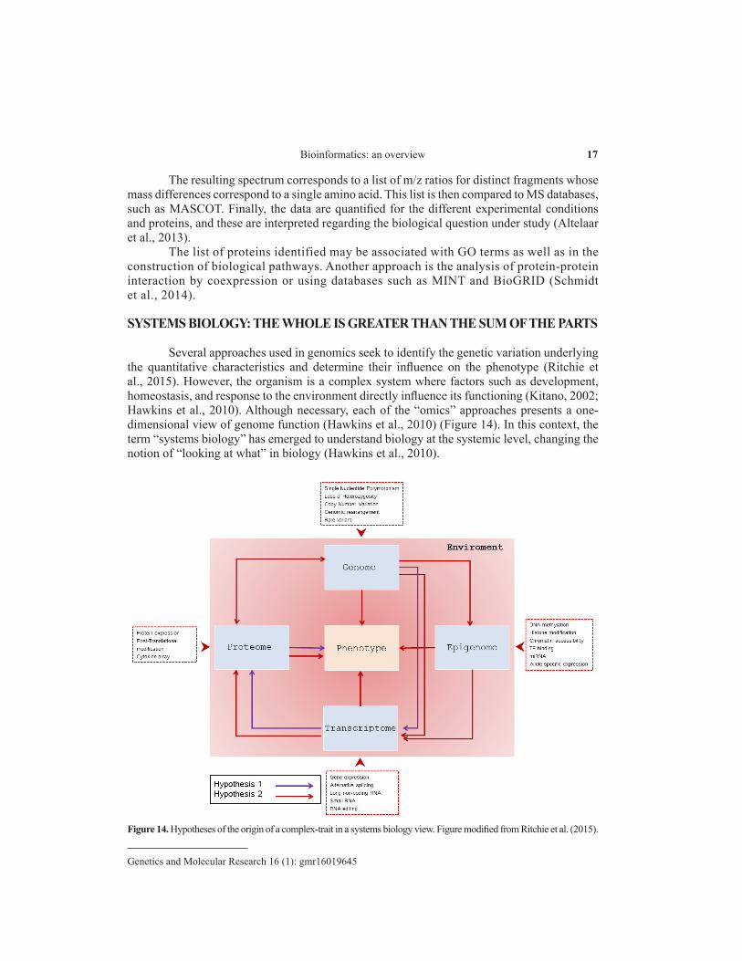
SYSTEMS BIOLOGY: THE WHOLE IS GREATER THAN THE SUM OF THE PARTS

Several approaches used in genomics seek to identify the genetic variation underlying the quantitative characteristics and determine their influence on the phenotype (Ritchie et al., 2015). However, the organism is a complex system where factors such as development, homeostasis, and response to the environment directly influence its functioning (Kitano, 2002; Hawkins et al., 2010). Although necessary, each of the “omics” approaches presents a one-dimensional view of genome function (Hawkins et al., 2010) (Figure 14). In this context, the term “systems biology” has emerged to understand biology at the systemic level, changing the notion of “looking at what” in biology (Hawkins et al., 2010).

Figure 14. Hypotheses of the origin of a complex-trait in a systems biology view. Figure modified from Ritchie et al. (2015).



Systems biology presents a holistic approach to deciphering the complexity of the system, in which “the whole is greater than the sum of its parts” (Institute for Systems Biology, 2016). This is a multidisciplinary science to develop new technologies, to explore the new dimension of data, to generate new discoveries and hypotheses, creating a cycle of innovation (Figure 15).

The systems approach at the genomic level makes it possible to reach complete and informative questions about genotype-phenotype associations when compared to a single data analysis (Ritchie et al., 2015). Identifying genes and proteins is important, although it is not enough to understand the complexity of the system. The comprehension of the system can be derived from the understanding of four key properties: the structure, the dynamics, the method of control, and the design of the method (Kitano, 2002).

Figure 15. Systems biology as a multidisciplinary science. Figure modified from Institute for Systems Biology (2016).

Faced with an explosion of available data, combining them can compensate the missing or unreliable information so that many evidence with the same targeting will be less susceptible to false positives. Besides, understanding a particular biological model is only possible if the different levels of regulation (genetics, genomics, and proteomics) are considered concomitantly in the analysis (Ritchie et al., 2015). Thus, data integration emerges to link our ability to generate large amounts of data to our understanding of biology, making it possible to identify key genomic factors and their interactions that explain the biological result.



Ritchie et al. (2015) classify data integration methods under two approaches: i) multistage analysis where only two different scales are used at a time to construct the models, considering a hierarchical or linear mode (e.g., SNPs and gene expression). Moreover, ii) multidimensional analyses in which all data sets are combined simultaneously to determine complex models. Still, the choice of method depends on two primary molecular hypotheses (Figure 14). The standard model is that changes in DNA will cause changes in gene expression and consequently in protein and phenotype (hypothesis 1). Otherwise, hypothesis 2 indicates that molecular variations at multiple levels contribute to the determination of the phenotype (Ritchie et al., 2015).

An overview of data integration: the use of networks

Differential expression studies have been widely adopted as a method to investigate the functions of genes on a global scale. In this approach, the genes are treated individually, without considering the interactions between them (Hong et al., 2013). However, biological functions exhibit a complex behavior, resulting from a set of genes interacting with each other (Zhao et al., 2010). In this context, the integrated biological systems approach using gene networks of coexpression has been widely used to understand the genetic architecture of complex phenotypes (Xu et al., 2014).

Different levels of information can be integrated with networks. For example, the body is made of multiple networks (genes, molecular, cellular, and organ networks) that are incorporated and communicate at multiple scales (Institute for Systems Biology, 2016). Among the multiple approaches that can be used in the identification of biological networks, the use of genetic coexpression networks as multistage analysis method will be highlighted.

In this analysis, it is assumed that all genes (nodes) are connected, and their connection strength (connectivity) is quantified by the correlation of the expression between them (Zhao et al., 2010). Thus, it is possible to detect groups of highly coexpressed genes (modules) that share a common function for which they are believed to act cooperatively (guilt by association) in a metabolic pathway (Kogelman et al., 2014). The connectivity of the gene (ki) describes the relative importance of the gene in the network. Genes with high ki are biologically relevant and reflect heavily regulated processes (Kogelman et al., 2014). Since the modules may correspond to biological pathways, it is possible to investigate whether the modules identified are associated with certain phenotypes as well as the significance of the gene on the traits under analysis (Zhao et al., 2010). This analysis is an assumption of the WGCNA software (Weighted Gene Co-expression Network Analysis). The detailed description of other methods of data analysis can be obtained in Ritchie et al. (2015).

CONSIDERATIONS AND PERSPECTIVES

Advances in the capabilities of data generation and analysis, as well as in the interpretation of results, have pointed to a promising future. However, wide progress in all areas of science highlights the emergence of new analytical strategies. While expanding our understanding of how the body works, the use of information at the molecular level should move to systemic approaches, promising to transform our understanding of the regulation of complex biological systems. On the other hand, data integration is not the end. It is the beginning of new discoveries and hypotheses, generating a feedback system. Moreover, major advances in health will be obtained, such as the use of genomic technologies in gene therapy and



personalized medicine. This prospect points out the need for scientists with mastery in multiple areas of knowledge, as well as the performance of multidisciplinary research groups, in which the complementarity of the different abilities will allow remarkable advances in science.

Conflicts of interest

The authors declare no conflict of interest.

REFERENCES

Altelaar AFM, Munoz J and Heck AJR (2013). Next-generation proteomics: towards an integrative view of proteome dynamics. Nat. Rev. Genet. 14: 35-48 http://dx.doi.org/10.1038/nrg3356.

Altmann A, Weber P, Bader D, Preuss M, et al. (2012). A beginners guide to SNP calling from high-throughput DNA-sequencing data. Hum. Genet. 131: 1541-1554 http://dx.doi.org/10.1007/s00439-012-1213-z.

Amaral AM, Reis MS and Silva FR (2007). O programa BLAST: guia prático de utilização. 1st edn. Embrapa Recursos Genéticos e Biotecnologia. EMBRAPA, Brasília.

Calixto PHM (2013). Aspectos gerais sobre a modelagem comparativa de proteínas. Cienc. Equat. 3: 10-16.Capriles PVSZ, Trevizani R, Rocha GK and Dardenne LE (2014). Modelos tridimensionais. In: Bioinformática da biologia

à flexibilidade molecular (Verli H, ed.). SBBq, São Paulo, 147-171.Chaisson MJP, Wilson RK and Eichler EE (2015). Genetic variation and the de novo assembly of human genomes. Nat.

Rev. Genet. 16: 627-640 http://dx.doi.org/10.1038/nrg3933.Daugelaite J, O’ Driscoll A and Sleator RD (2013). An overview of multiple sequence alignments and cloud computing in

bioinformatics. Int. Sch. Res. Not. e615630. doi:10.1155/2013/615630.Dayhoff MO, Schwartz R and Orcutt BC (1978). A model of evolutionary change in proteins. Atlas of Protein Sequence

and Structure (volume 5, supplement 3 ed.). Nat. Biomed. Res. Found., Washington, D.C.Goff LA, Trapnell C and Kelley D (2012). CummeRbund : visualization and exploration of Cufflinks high-throughput

sequencing data. R package version 2.16.0.Hagen JB (2000). The origins of bioinformatics. Nat. Rev. Genet. 1: 231-236 http://dx.doi.org/10.1038/35042090.Hawkins RD, Hon GC and Ren B (2010). Next-generation genomics: an integrative approach. Nat. Rev. Genet. 11: 476-

486 10.1038/nrg2795.Hong S, Chen X, Jin L and Xiong M (2013). Canonical correlation analysis for RNA-seq co-expression networks. Nucleic

Acids Res. 41: e95 http://dx.doi.org/10.1093/nar/gkt145.Hunt LT (1984). Margaret Oakley Dayhoff 1925-1983. Bull. Math. Biol. 46: 467-472 http://dx.doi.org/10.1007/

BF02459497.Institute for Systems Biology (2016). What is a systems biology. institute for systems biology. Available at [https://www.

systemsbiology.org/about/what-is-systems-biology/].Jensen ON (2006). Interpreting the protein language using proteomics. Nat. Rev. Mol. Cell Biol. 7: 391-403 http://dx.doi.

org/10.1038/nrm1939.Junqueira DM, Braun RL and Verli H (2014). Alinhamentos. In: Bioinformática da biologia à flexibilidade molecular

(Verli H, ed.). SBBq, São Paulo, 38-61.Kitano H (2002). Systems biology: a brief overview. Science 295: 1662-1664 http://dx.doi.org/10.1126/science.1069492.Kogelman LJA, Cirera S, Zhernakova DV, Fredholm M, et al. (2014). Identification of co-expression gene networks,

regulatory genes and pathways for obesity based on adipose tissue RNA Sequencing in a porcine model. BMC Med. Genomics 7: 57 http://dx.doi.org/10.1186/1755-8794-7-57.

Luscombe NM, Greenbaum D and Gerstein M (2001). What is bioinformatics? A proposed definition and overview of the field. Methods Inf. Med. 40: 346-358 10.1053/j.ro.2009.03.010.

Madhusudhan MS, Marti-Renom MA and Eswar N (2005). Comparative protein structure modeling. In: The proteomics protocols handbook (Walker, J.M., ed.). Human Press, New Jersey, 831-860.

Malone JH and Oliver B (2011). Microarrays, deep sequencing and the true measure of the transcriptome. BMC Biol. 9: 34 http://dx.doi.org/10.1186/1741-7007-9-34.

Manohar P and Shailendra S (2012). Protein sequence alignment: A review. World Appl. Program. 2: 141-145.Marioni JC, Mason CE, Mane SM, Stephens M, et al. (2008). RNA-seq: an assessment of technical reproducibility and

comparison with gene expression arrays. Genome Res. 18: 1509-1517 http://dx.doi.org/10.1101/gr.079558.108.



Miller JR, Koren S and Sutton G (2010). Assembly algorithms for next-generation sequencing data. Genomics 95: 315-327 http://dx.doi.org/10.1016/j.ygeno.2010.03.001.

Montgomery SB, Sammeth M, Gutierrez-Arcelus M, Lach RP, et al. (2010). Transcriptome genetics using second generation sequencing in a Caucasian population. Nature 464: 773-777 http://dx.doi.org/10.1038/nature08903.

Pevsner J (2009). Pairwise sequence alignment. Bioinformatics and Functional Genomics (2nd edn). Wiley-Blackwell.Pevsner J (2015). Bioinformatics and functional genomics, 3rd ed. John Wiley & Sons Inc, Chichester.Prosdocimi F (2010). Introdução à bioinformática. Curso Online. Available at [http://www2.bioqmed.ufrj.br/prosdocimi/

FProsdocimi07_CursoBioinfo.pdf].Prosdocimi F, Cerqueira GC, Binneck E and Silva AF (2002). Bioinformática: Manual do usuário. Biotec. Cienc. Des.

12-25.Ritchie MD, Holzinger ER, Li R, Pendergrass SA, et al. (2015). Methods of integrating data to uncover genotype-

phenotype interactions. Nat. Rev. Genet. 16: 85-97 http://dx.doi.org/10.1038/nrg3868.Schmidt A, Forne I and Imhof A (2014). Bioinformatic analysis of proteomics data. BMC Syst. Biol. 8: 2, S3.

doi:10.1186/1752-0509-8-S2-S3.Silva VB and Silva CHT (2007). Modelagem molecular de proteínas-alvo por homologia estrutural. Rev. Elet. Farm. 4:

15-26.Sims D, Sudbery I, Ilott NE, Heger A, et al. (2014). Sequencing depth and coverage: key considerations in genomic

analyses. Nat. Rev. Genet. 15: 121-132 http://dx.doi.org/10.1038/nrg3642.Sung WK (2010). Algorithms in Bioinformatics: a practical introduction. CRC Press.Staats CC, Morais GL de and Margis R (2014). Projetos genoma. In: Bioinformática da biologia à flexibilidade molecular

(Verli H, ed.). SBBq, São Paulo, 62-79.Trapnell C, Pachter L and Salzberg SL (2009). TopHat: discovering splice junctions with RNA-Seq. Bioinformatics 25:

1105-1111 http://dx.doi.org/10.1093/bioinformatics/btp120.Trapnell C, Roberts A, Goff L, Pertea G, et al. (2012). Differential gene and transcript expression analysis of RNA-seq

experiments with TopHat and Cufflinks. Nat. Protoc. 7: 562-578 http://dx.doi.org/10.1038/nprot.2012.016.Verli H (2014). O que é Bioinformática? In: Bioinformática da biologia à flexibilidade molecular (Verli H ed.). SBBq,

São Paulo, 1-12.Wang J (2009). Protein structure prediction by comparative modeling: an analysis of methodology. Comp. Gen. Pharmacol.

218: 1-13.Wang Z, Gerstein M and Snyder M (2009). RNA-Seq: a revolutionary tool for transcriptomics. Nat. Rev. Genet. 10: 57-63

http://dx.doi.org/10.1038/nrg2484.Xu L, Zhao F, Ren H, Li L, et al. (2014). Co-expression analysis of fetal weight-related genes in ovine skeletal muscle

during mid and late fetal development stages. Int. J. Biol. Sci. 10: 1039-1050 http://dx.doi.org/10.7150/ijbs.9737.Zhao W, Langfelder P, Fuller T, Dong J, et al. (2010). Weighted gene coexpression network analysis: state of the art. J.

Biopharm. Stat. 20: 281-300 http://dx.doi.org/10.1080/10543400903572753.Zhou X, Ren L, Meng Q, Li Y, et al. (2010). The next-generation sequencing technology and application. Protein Cell 1:

520-536 http://dx.doi.org/10.1007/s13238-010-0065-3.

bioinformatics: an overview and its applications - … · still, in bioinformatics, development of...

Documents