biogeosciences evaluating the agreement between …faculty.geog.utoronto.ca/chen/chen's...

Biogeosciences, 10, 6893–6909, 2013www.biogeosciences.net/10/6893/2013/doi:10.5194/bg-10-6893-2013© Author(s) 2013. CC Attribution 3.0 License.

Biogeosciences

Open A

ccess

Evaluating the agreement between measurements and models of netecosystem exchange at different times and timescales using waveletcoherence: an example using data from the North American CarbonProgram Site-Level Interim Synthesis

P. C. Stoy1, M. C. Dietze2, A. D. Richardson3, R. Vargas4, A. G. Barr 5, R. S. Anderson6, M. A. Arain 7, I. T. Baker8,T. A. Black9, J. M. Chen10, R. B. Cook11, C. M. Gough12, R. F. Grant13, D. Y. Hollinger14, R. C. Izaurralde15,C. J. Kucharik 16, P. Lafleur17, B. E. Law18, S. Liu19, E. Lokupitiya 20, Y. Luo21, J. W. Munger22, C. Peng23,B. Poulter24, D. T. Price25, D. M. Ricciuto11, W. J. Riley26, A. K. Sahoo27, K. Schaefer28, C. R. Schwalm29, H. Tian30,H. Verbeeck31, and E. Weng32

1Department of Land Resources and Environmental Sciences, Bozeman, MT 59717, USA2Department of Earth and Environment, Boston University, Boston, MA 02215, USA3Department of Organismic & Evolutionary Biology, Harvard University, Cambridge, MA 02138, USA4Department of Plant and Soil Sciences, Delaware Environmental Institute, University of Delaware, Newark, DE 19717, USA5Climate Research Division, Atmospheric Science and Technology Directorate, Saskatoon, SK S7N 3H5, Canada6Numerical Terradynamic Simulation Group, University of Montana, Missoula, MT 59812, USA7School of Geography and Earth Sciences and McMaster Centre for Climate Change, McMaster University, Hamilton, ONL8S 4K1, Canada8Department of Atmospheric Science, Colorado State University, Fort Collins, CO 80523, USA9Faculty of Land and Food Systems, University of British Columbia, Vancouver, BC V6T 1Z4, Canada10Department of Geography and Program in Planning, University of Toronto, Toronto, ON M5S 3G3, Canada11Environmental Sciences Division, Oak Ridge National Laboratory, Oak Ridge, TN 37831, USA12Department of Biology, Virginia Commonwealth University, Richmond, VA 23284, USA13Department of Renewable Resources, University of Alberta, Edmonton, AB T6G 2E3, Canada14Northern Research Station, USDA Forest Service, Durham, NH 03824, USA15Pacific Northwest National Laboratory and University of Maryland, College Park, MD 20740, USA16Department of Agronomy & Nelson Institute Center for Sustainability and the Global Environment, University ofWisconsin – Madison, Madison, WI 53706, USA17Department of Geography, Trent University, Peterborough, ON K9J 7B8, Canada18Department of Forest Ecosystems and Society, Oregon State University, Corvallis, OR 97331, USA19US Geological Survey (USGS) Earth Resources Observation and Science (EROS) Center, Sioux Falls, SD 57198, USA20Department of Zoology, POB 1490, University of Colombo, Colombo 03, Sri Lanka21Department of Botany and Microbiology, University of Oklahoma, Norman, OK 73019, USA22School of Engineering and Applied Sciences and Department of Earth and Planetary Sciences, Harvard University,Cambridge, MA 02138, USA23Department of Biology Sciences, University of Quebec at Montreal, Montreal, QC H3C 3P8, Canada24Laboratoire des Sciences du Climat et de l’Environnement, Gif-sur-Yvette, France25Northern Forestry Centre, Canadian Forest Service, Edmonton, AB T6H 3S5, Canada26Climate and Carbon Sciences, Earth Sciences Division, Lawrence Berkeley National Laboratory, Berkeley, CA 94720, USA27Department of Civil and Environmental Engineering, Princeton University, Princeton, NJ 08544, USA28National Snow and Ice Data Center (NSIDC), University of Colorado, Boulder, CO 80309, USA29School of Earth Science and Environmental Sustainability, Northern Arizona University, Flagstaff, AZ 86001, USA30School of Forestry and Wildlife Sciences, Auburn University, Auburn, AL 36849, USA

Published by Copernicus Publications on behalf of the European Geosciences Union.

6894 P. C. Stoy et al.: Wavelet coherence for multiple models

31Laboratory of Plant Ecology, Ghent University, 9000 Ghent, Belgium32Department of Ecology and Evolutionary Biology, Princeton University, Princeton, NJ 08544, USA

Correspondence to: P. C. Stoy ([email protected])

Received: 16 January 2013 – Published in Biogeosciences Discuss.: 19 February 2013Revised: 24 September 2013 – Accepted: 29 September 2013 – Published: 4 November 2013

Abstract. Earth system processes exhibit complex patternsacross time, as do the models that seek to replicate theseprocesses. Model output may or may not be significantly re-lated to observations at different times and on different fre-quencies. Conventional model diagnostics provide an aggre-gate view of model–data agreement, but usually do not iden-tify the time and frequency patterns of model–data disagree-ment, leaving unclear the steps required to improve modelresponse to environmental drivers that vary on characteristicfrequencies. Wavelet coherence can quantify the times andtimescales at which two time series, for example time se-ries of models and measurements, are significantly different.We applied wavelet coherence to interpret the predictionsof 20 ecosystem models from the North American CarbonProgram (NACP) Site-Level Interim Synthesis when con-fronted with eddy-covariance-measured net ecosystem ex-change (NEE) from 10 ecosystems with multiple years ofavailable data. Models were grouped into classes with simi-lar approaches for incorporating phenology, the calculationof NEE, the inclusion of foliar nitrogen (N), and the useof model–data fusion. Models with prescribed, rather thanprognostic, phenology often fit NEE observations better onannual to interannual timescales in grassland, wetland andagricultural ecosystems. Models that calculated NEE as netprimary productivity (NPP) minus heterotrophic respiration(HR) rather than gross ecosystem productivity (GPP) minusecosystem respiration (ER) fit better on annual timescalesin grassland and wetland ecosystems, but models that cal-culated NEE as GPP minus ER were superior on monthlyto seasonal timescales in two coniferous forests. Modelsthat incorporated foliar nitrogen (N) data were successfulat capturing NEE variability on interannual (multiple year)timescales at Howland Forest, Maine. The model that em-ployed a model–data fusion approach often, but not always,resulted in improved fit to data, suggesting that improvingmodel parameterization is important but not the only stepfor improving model performance. Combined with previ-ous findings, our results suggest that the mechanisms drivingdaily and annual NEE variability tend to be correctly simu-lated, but the magnitude of these fluxes is often erroneous,suggesting that model parameterization must be improved.Few NACP models correctly predicted fluxes on seasonaland interannual timescales where spectral energy in NEE ob-servations tends to be low, but where phenological events,

multi-year oscillations in climatological drivers, and ecosys-tem succession are known to be important for determiningecosystem function. Mechanistic improvements to modelsmust be made to replicate observed NEE variability on sea-sonal and interannual timescales.

1 Introduction

Land surface models represent our understanding of howterrestrial ecosystems function in the climate system. It iscritical to test, compare, and improve these models as newinformation and methods become available, especially be-cause numerous recent syntheses have demonstrated a con-siderable lack of model skill when confronted with observa-tions (Schwalm et al., 2010; Wang et al., 2010; Schaefer etal., 2012). Models are commonly diagnosed using statisti-cal metrics that can be combined for a more complete viewof model performance (Taylor, 2001). Such model diagnos-tics are able to identify whether a different model, differentmodel parameterization, or different subroutine represents animprovement (Akaike, 1974), but are not intended to iden-tify the symptoms of model–data disagreement across timeand scales in time in order to identify the conditions that re-sult in discrepancies. Residual analyses and detailed inves-tigations of model performance during different time peri-ods give important insight into the mechanisms underlyingmodel failure, but are rarely interpreted with respect to pat-terns of model/measurement mismatch in the frequency (ortimescale) domain (see howeverDietze et al., 2011; Mahechaet al., 2010; Vargas et al., 2010, andVargas et al., 2013). Inthis paper, we quantify periods in time and scales in timewhen ecosystem models are not significantly related to eddycovariance measurements of net ecosystem exchange (NEE)to identify periods in which models can and should be im-proved (Williams et al., 2009).

Improving individual models is a noteworthy goal, butmodern studies often combine multiple observations andmultiple model simulations (i.e., multiple databases) to ar-rive at a synthesis (Friedlingstein et al., 2006; Schwalm etal., 2010). In other words, such studies adopt a data-intensiveapproach to scientific inference (Gray, 2009), and techniquesfrom nonlinear time-series analysis and knowledge discov-ery in databases (i.e., “data mining”) may provide important

Biogeosciences, 10, 6893–6909, 2013 www.biogeosciences.net/10/6893/2013/

P. C. Stoy et al.: Wavelet coherence for multiple models 6895

insights into the aggregate or divergent behavior of thesemodel and observational databases. In this study, we quan-tify significant relationships among 20 ecosystem modelsand 10 multi-year time series of NEE measurements from theNorth American Carbon Program (NACP) Site-Level InterimSynthesis (Schwalm et al., 2010) using a technique calledwavelet coherence (Grinsted et al., 2004; Torrence and Web-ster, 1999). Wavelet coherence is conceptually similar to ameasure of correlation between data series across time andtimescale (related to frequency). Like correlation, significantvalues of wavelet coherence can be quantified, in this case bycomparison against appropriate synthetic null spectra. Un-like simple correlation, statistical significance can be quan-tified across both time and timescales simultaneously. Weuse wavelet coherence to determine the times and timescaleswhen NACP models and measurements are significantly re-lated and, more importantly, when they are not. Notably,wavelet coherence can quantify significance in the time andtimescale domains even when common power (i.e., sharedvariability) among time series on these scales is low (Grin-sted et al., 2004), and may offer an improvement over resid-ual analyses for this reason. Wavelet coherence has foundapplications in comparing ecological models and measure-ments for the goal of model improvement (Williams et al.,2009; Wang et al., 2011), but not across multiple model andobservational time series to date.

Previous studies of ecosystem models in the timescale do-main have demonstrated that models tend to miss patterns influx observations on intermediate (i.e., weekly to monthly)and interannual timescales (Siqueira et al., 2006; Stoy et al.,2005). Biological responses to variability in climate oftendominates flux variability on these timescales (Richardson etal., 2007), and models tend to replicate this biological func-tioning poorly. Such responses include weekly to monthlyshifts in leaf-out/leaf-drop phenology and the multitude offactors, including lagged responses, known to contribute tointerannual carbon flux variability (Richardson et al., 2013).With respect to the NACP, findings to date have identifiedsuperior model fit when phenology is prescribed by remotesensing observations as opposed to prognostic via a phenol-ogy model, when a sub-daily (i.e., half hourly or hourly)rather than a daily time step is used, and when net ecosys-tem exchange (NEE) is calculated as the difference betweengross primary productivity (GPP) and ecosystem respiration(ER) rather than the difference between net primary produc-tivity (NPP) and heterotrophic respiration (HR) (Schwalm etal., 2010; Richardson et al., 2012). Schwalm et al.(2010)also found that model performance was poorer during springand fall when phenological events dominate surface flux andduring dry periods within the growing season. Less certain ishow models match measurements on multiple timescales asthey respond to climatic and biological forcings that act onmultiple timescales (Dietze et al., 2011). Quantifying suchmodel–measurement relationships contributes to the NACPobjective to measure and understand the sources and sinks

of CO2 in North America. Following previous studies, wehypothesize that models will tend to match flux patterns ondaily and annual timescales, and we focus our investigationon timescales between weeks and multiple months as well asinterannual timescales, where we postulate that models willreplicate observations more poorly.

2 Methods

2.1 Eddy covariance data and ecosystem models

Half hourly (or hourly) micrometeorological and eddy co-variance measurements were collected by site principalinvestigators and research teams and were provided tothe AmeriFlux and Fluxnet-Canada consortia to create theNACP Site Level Interim Synthesis product (Schwalm et al.,2010). For this analysis we examine 20 ecosystem modelsagainst measurements of the net ecosystem exchange of CO2(NEE) from the 10 eddy covariance research sites investi-gated byDietze et al.(2011) (Table1). These sites were cho-sen because the length of the observation period tended to belonger and more continuous, allowing us to investigate inter-annual (multiple year) variability, and because more modelstended to be run for these ecosystems (Schwalm et al., 2010;Schaefer et al., 2012). Missing meteorological data were gap-filled using National Oceanic and Atmospheric Administra-tion (NOAA) meteorological station data and Daymet reanal-ysis products (Ricciuto et al., 2009). Half-hourly (or hourly)NEE values were filtered to remove periods of insufficientturbulence determined using friction velocity (u∗) thresh-olds, and despiked to remove outliers (Papale et al., 2006;Reichstein et al., 2005). Missing NEE data were then gap-filled following Barr et al.(2009). We note that gap-fillingmodels tend to match closely the orthonormal wavelet coef-ficients of NEE measurements at timescales longer than oneday (Stoy et al., 2006), and thus gap-filling artifacts shouldhave minimal impact on our results. Model runs at each sitefollowed a prescribed protocol for intercomparison describedby Schwalm et al.(2010). Ancillary biological, disturbance,edaphic, and management data used by model runs for eachsite were given by the AmeriFlux BADM templates (Law etal., 2008). The ecosystem models explored here are listed inTable2 and described in more detail inSchwalm et al.(2010)and the original publications. Likewise, information regard-ing the study sites is best found in the original publications(Table1).

2.2 Wavelet coherence

The times and timescales at which two corresponding dataseries (here time series) have high common power can bequantified using the wavelet cospectrum. Wavelet coherenceuses wavelet spectral and cospectral calculations to quan-tify correlations in the time and timescale domains (Grin-sted et al., 2004; Torrence and Webster, 1999), and we refer

www.biogeosciences.net/10/6893/2013/ Biogeosciences, 10, 6893–6909, 2013


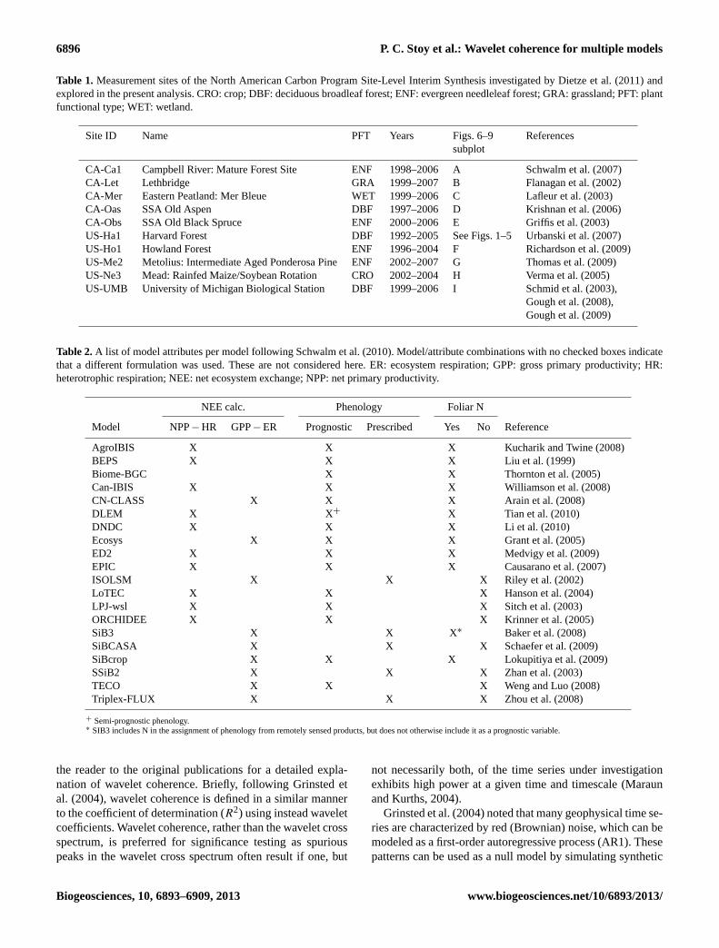
Table 1. Measurement sites of the North American Carbon Program Site-Level Interim Synthesis investigated byDietze et al.(2011) andexplored in the present analysis. CRO: crop; DBF: deciduous broadleaf forest; ENF: evergreen needleleaf forest; GRA: grassland; PFT: plantfunctional type; WET: wetland.

Site ID Name PFT Years Figs. 6–9 Referencessubplot

CA-Ca1 Campbell River: Mature Forest Site ENF 1998–2006 A Schwalm et al.(2007)CA-Let Lethbridge GRA 1999–2007 B Flanagan et al.(2002)CA-Mer Eastern Peatland: Mer Bleue WET 1999–2006 C Lafleur et al.(2003)CA-Oas SSA Old Aspen DBF 1997–2006 D Krishnan et al.(2006)CA-Obs SSA Old Black Spruce ENF 2000–2006 E Griffis et al.(2003)US-Ha1 Harvard Forest DBF 1992–2005 See Figs. 1–5Urbanski et al.(2007)US-Ho1 Howland Forest ENF 1996–2004 F Richardson et al.(2009)US-Me2 Metolius: Intermediate Aged Ponderosa Pine ENF 2002–2007 G Thomas et al.(2009)US-Ne3 Mead: Rainfed Maize/Soybean Rotation CRO 2002–2004 H Verma et al.(2005)US-UMB University of Michigan Biological Station DBF 1999–2006 I Schmid et al.(2003),

Gough et al.(2008),Gough et al.(2009)

Table 2.A list of model attributes per model followingSchwalm et al.(2010). Model/attribute combinations with no checked boxes indicatethat a different formulation was used. These are not considered here. ER: ecosystem respiration; GPP: gross primary productivity; HR:heterotrophic respiration; NEE: net ecosystem exchange; NPP: net primary productivity.

NEE calc. Phenology Foliar N

Model NPP− HR GPP− ER Prognostic Prescribed Yes No Reference

AgroIBIS X X X Kucharik and Twine(2008)BEPS X X X Liu et al. (1999)Biome-BGC X X Thornton et al.(2005)Can-IBIS X X X Williamson et al.(2008)CN-CLASS X X X Arain et al.(2008)DLEM X X + X Tian et al.(2010)DNDC X X X Li et al. (2010)Ecosys X X X Grant et al.(2005)ED2 X X X Medvigy et al.(2009)EPIC X X X Causarano et al.(2007)ISOLSM X X X Riley et al.(2002)LoTEC X X X Hanson et al.(2004)LPJ-wsl X X X Sitch et al.(2003)ORCHIDEE X X X Krinner et al.(2005)SiB3 X X X∗ Baker et al.(2008)SiBCASA X X X Schaefer et al.(2009)SiBcrop X X X Lokupitiya et al.(2009)SSiB2 X X X Zhan et al.(2003)TECO X X X Weng and Luo(2008)Triplex-FLUX X X X Zhou et al.(2008)

+ Semi-prognostic phenology.∗ SIB3 includes N in the assignment of phenology from remotely sensed products, but does not otherwise include it as a prognostic variable.

the reader to the original publications for a detailed expla-nation of wavelet coherence. Briefly, followingGrinsted etal. (2004), wavelet coherence is defined in a similar mannerto the coefficient of determination (R2) using instead waveletcoefficients. Wavelet coherence, rather than the wavelet crossspectrum, is preferred for significance testing as spuriouspeaks in the wavelet cross spectrum often result if one, but

not necessarily both, of the time series under investigationexhibits high power at a given time and timescale (Maraunand Kurths, 2004).

Grinsted et al.(2004) noted that many geophysical time se-ries are characterized by red (Brownian) noise, which can bemodeled as a first-order autoregressive process (AR1). Thesepatterns can be used as a null model by simulating synthetic



data that were simulated with AR1 coefficients to quantifysignificant wavelet coherence at the 95 % confidence level.Eddy covariance time series approximate pink noise (1/f

noise) (Richardson et al., 2008), which is likewise a classof autoregressive noise, andGrinsted et al.(2004) demon-strated that the color of noise has little impact on the deter-mination of the significance level. Wavelet coherence valuesabove 0.7 were found byGrinsted et al.(2004) to be signifi-cant against synthetic data sets across a wide range of scaleswhen ten scales per octave (i.e., per a doubling or halvingof frequency) were chosen in the scale-wise smoothing, al-though higher coherence values (ca. 0.8 or higher) shouldbe chosen at very high and low frequencies. We used tenscales per octave and also chose the commonly used 0.7wavelet coherence threshold for determining significance.We de-emphasize the interpretation of high-frequency co-herence (e.g., on hourly and sub-daily timescales) to focuson the longer timescales (i.e.,> one day) where models of-ten fail. Wavelet coefficients on very long timescales (yearsto multiple years) often exceed the so-called cone of influ-ence beyond which the coherence calculation is dominatedby edge effects because of incomplete time locality acrossfrequencies (Torrence and Compo, 1998). Wavelet coeffi-cients outside the cone of influence are unreliable and willnot be interpreted here. Also for consistency withGrinsted etal. (2004), we chose the Morlet wavelet basis function with awave number of six. Time series were truncated to powers oftwo for spectral calculations. Further, it is common to presentwavelet coefficients as the absolute value of their real andimaginary components along time and frequency axes: theso-called wavelet half-plane. Here, we present wavelet coher-ence values in a similar manner along the time and timescaleaxes.

The dimensions of time and timescale (subsequentlycalled “regions”) adjudged to be significant may occasionallybe larger than uncertainty bounds on account of autocorrela-tion in time and timescale (Maraun et al., 2007). As a conse-quence, we advocate a conservative analysis of the precise di-mensions of regions adjudged to have significant coherence,and we do not seek here to interpret the dimensions of allregions here, rather the existence of significant wavelet co-herence. We also note that, following the Monte Carlo analy-sis, significant wavelet coherence may occur by chance. Ouranalysis focuses on regions where models and measurementsdo not exhibit significant coherence under the expectationthat models should match measurements, and with the un-derstanding that one learns more about a given system whenmodels fail.

Results are presented with two different representations oftimescale in mind. For the demonstration of the wavelet co-herence technique, we interpret all relevant scales from twicethe observation time step (usually 1 to 2 hours) to half thelength of the truncated time series. For the comparison ofmodel output against flux observations, we interpret waveletcoherence on timescales longer than one day to enable a com-

parison among models that operate on daily and sub-dailytime steps and to focus our analysis on the longer timescales(e.g., seasonal or interannual timescales) on which modelsoften fail.

2.2.1 Combined wavelet coherence significance analysis

A time–timescale graph of wavelet coherence significancevalues can be created for each model–measurement combi-nation for each site. As such, significance values from dif-ferent models run for a single site that lie upon identicalaxes can be combined for an aggregate view of model perfor-mance. The approach that we explore is to sum wavelet co-efficients that represent significance values at different timesand timescales (i) for models that possess a given attributeA (Ai), divide by the number of models withA (NA), thensubtract the sum of the wavelet coherence significance valuesfor models that possess the opposing model attributeB (Bi)divided by the number of models withB (NB ):

1

NA

NA∑i=1

Ai −1

NB

NB∑i=1

Bi . (1)

The purpose of this calculation is to provide a simple met-ric between−1 and 1 for cases whereNA andNB may be dif-ferent but are weighted equally to simplify comparison. Thegoal is to identify regions in time and timescale at differentsites where a certain model attribute outperforms the other(or others) across all models investigated here, with the goalof interpreting the success or failure of different model for-mulations across time and timescale for different ecosystemtypes. An infinite number of alternate approaches to comparemultiple models exists. To avoid over-interpreting results andto simplify the visual display, we only plot absolute valuesof Eq. (1) that exceed 0.33 to focus our study on times andtimescales where the first and second terms of Eq. (1) differby at least one-third.

3 Results and discussion

3.1 Wavelet coherence

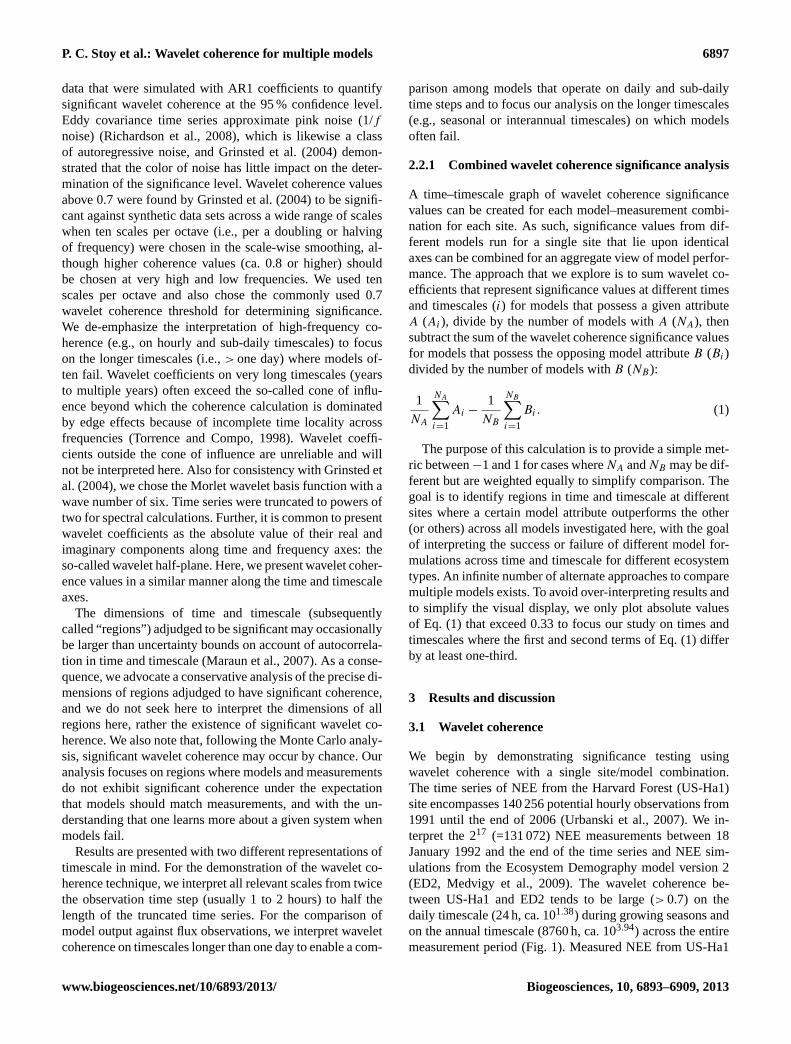
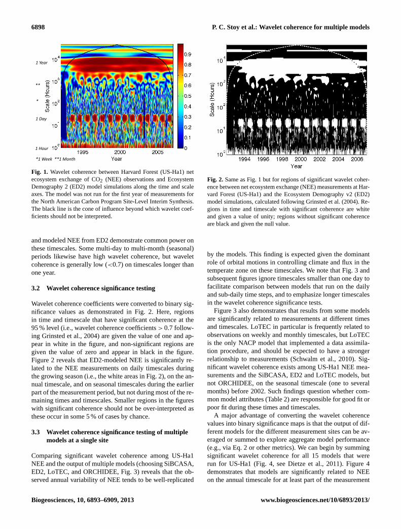
We begin by demonstrating significance testing usingwavelet coherence with a single site/model combination.The time series of NEE from the Harvard Forest (US-Ha1)site encompasses 140 256 potential hourly observations from1991 until the end of 2006 (Urbanski et al., 2007). We in-terpret the 217 (=131 072) NEE measurements between 18January 1992 and the end of the time series and NEE sim-ulations from the Ecosystem Demography model version 2(ED2, Medvigy et al., 2009). The wavelet coherence be-tween US-Ha1 and ED2 tends to be large (> 0.7) on thedaily timescale (24 h, ca. 101.38) during growing seasons andon the annual timescale (8760 h, ca. 103.94) across the entiremeasurement period (Fig.1). Measured NEE from US-Ha1



1 Hour

1 Day

*1 Week **1 Month

*

**

1 Year

Fig. 1. Wavelet coherence between Harvard Forest (US-Ha1) netecosystem exchange of CO2 (NEE) observations and EcosystemDemography 2 (ED2) model simulations along the time and scaleaxes. The model was not run for the first year of measurements forthe North American Carbon Program Site-Level Interim Synthesis.The black line is the cone of influence beyond which wavelet coef-ficients should not be interpreted.

and modeled NEE from ED2 demonstrate common power onthese timescales. Some multi-day to multi-month (seasonal)periods likewise have high wavelet coherence, but waveletcoherence is generally low (<0.7) on timescales longer thanone year.

3.2 Wavelet coherence significance testing

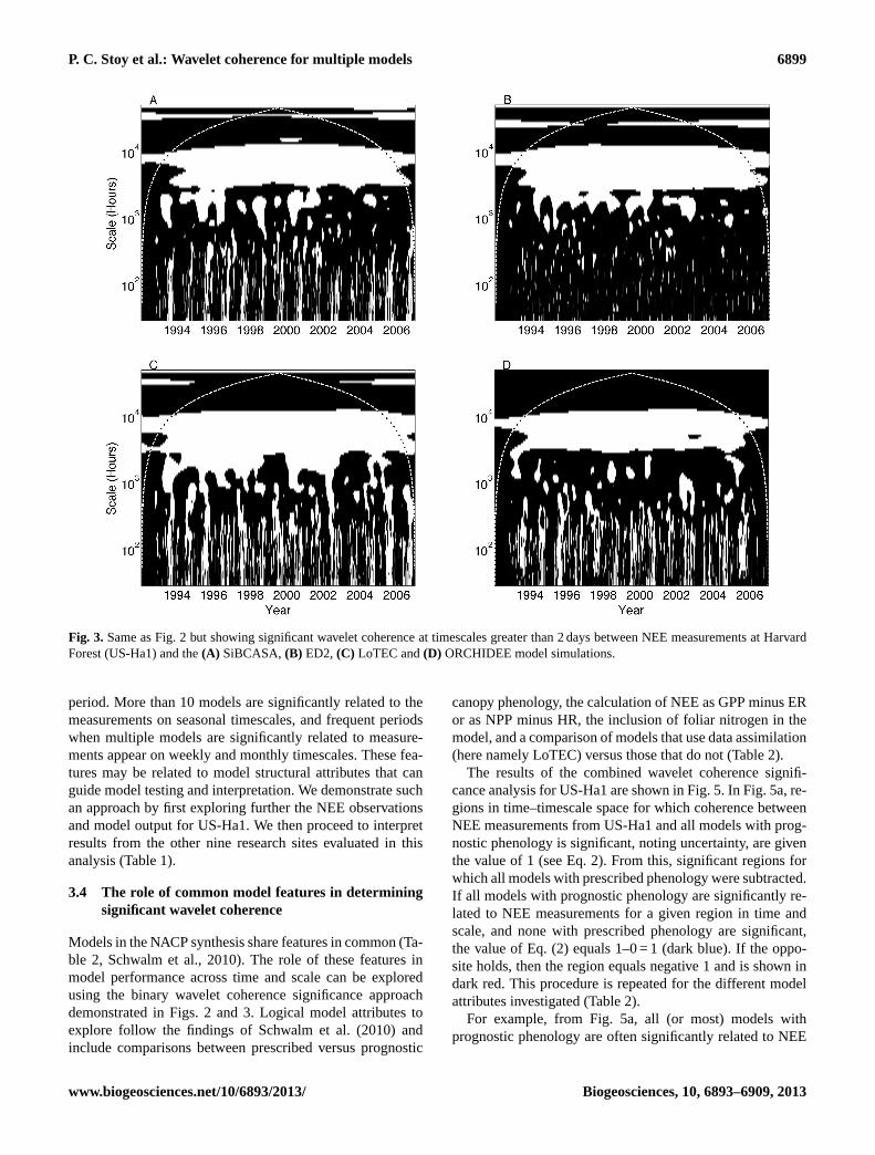
Wavelet coherence coefficients were converted to binary sig-nificance values as demonstrated in Fig.2. Here, regionsin time and timescale that have significant coherence at the95 % level (i.e., wavelet coherence coefficients> 0.7 follow-ing Grinsted et al., 2004) are given the value of one and ap-pear in white in the figure, and non-significant regions aregiven the value of zero and appear in black in the figure.Figure2 reveals that ED2-modeled NEE is significantly re-lated to the NEE measurements on daily timescales duringthe growing season (i.e., the white areas in Fig.2), on the an-nual timescale, and on seasonal timescales during the earlierpart of the measurement period, but not during most of the re-maining times and timescales. Smaller regions in the figureswith significant coherence should not be over-interpreted asthese occur in some 5 % of cases by chance.

3.3 Wavelet coherence significance testing of multiplemodels at a single site

Comparing significant wavelet coherence among US-Ha1NEE and the output of multiple models (choosing SiBCASA,ED2, LoTEC, and ORCHIDEE, Fig.3) reveals that the ob-served annual variability of NEE tends to be well-replicated

Fig. 2. Same as Fig. 1 but for regions of significant wavelet coher-ence between net ecosystem exchange (NEE) measurements at Har-vard Forest (US-Ha1) and the Ecosystem Demography v2 (ED2)model simulations, calculated followingGrinsted et al.(2004). Re-gions in time and timescale with significant coherence are whiteand given a value of unity; regions without significant coherenceare black and given the null value.

by the models. This finding is expected given the dominantrole of orbital motions in controlling climate and flux in thetemperate zone on these timescales. We note that Fig.3 andsubsequent figures ignore timescales smaller than one day tofacilitate comparison between models that run on the dailyand sub-daily time steps, and to emphasize longer timescalesin the wavelet coherence significance tests.

Figure3 also demonstrates that results from some modelsare significantly related to measurements at different timesand timescales. LoTEC in particular is frequently related toobservations on weekly and monthly timescales, but LoTECis the only NACP model that implemented a data assimila-tion procedure, and should be expected to have a strongerrelationship to measurements (Schwalm et al., 2010). Sig-nificant wavelet coherence exists among US-Ha1 NEE mea-surements and the SiBCASA, ED2 and LoTEC models, butnot ORCHIDEE, on the seasonal timescale (one to severalmonths) before 2002. Such findings question whether com-mon model attributes (Table2) are responsible for good fit orpoor fit during these times and timescales.

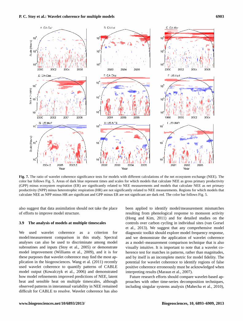
A major advantage of converting the wavelet coherencevalues into binary significance maps is that the output of dif-ferent models for the different measurement sites can be av-eraged or summed to explore aggregate model performance(e.g., via Eq. 2 or other metrics). We can begin by summingsignificant wavelet coherence for all 15 models that wererun for US-Ha1 (Fig.4, seeDietze et al., 2011). Figure4demonstrates that models are significantly related to NEEon the annual timescale for at least part of the measurement



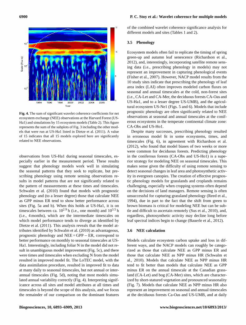
Fig. 3. Same as Fig. 2 but showing significant wavelet coherence at timescales greater than 2 days between NEE measurements at HarvardForest (US-Ha1) and the(A) SiBCASA, (B) ED2, (C) LoTEC and(D) ORCHIDEE model simulations.

period. More than 10 models are significantly related to themeasurements on seasonal timescales, and frequent periodswhen multiple models are significantly related to measure-ments appear on weekly and monthly timescales. These fea-tures may be related to model structural attributes that canguide model testing and interpretation. We demonstrate suchan approach by first exploring further the NEE observationsand model output for US-Ha1. We then proceed to interpretresults from the other nine research sites evaluated in thisanalysis (Table1).

3.4 The role of common model features in determiningsignificant wavelet coherence

Models in the NACP synthesis share features in common (Ta-ble 2, Schwalm et al., 2010). The role of these features inmodel performance across time and scale can be exploredusing the binary wavelet coherence significance approachdemonstrated in Figs. 2 and 3. Logical model attributes toexplore follow the findings ofSchwalm et al.(2010) andinclude comparisons between prescribed versus prognostic

canopy phenology, the calculation of NEE as GPP minus ERor as NPP minus HR, the inclusion of foliar nitrogen in themodel, and a comparison of models that use data assimilation(here namely LoTEC) versus those that do not (Table2).

The results of the combined wavelet coherence signifi-cance analysis for US-Ha1 are shown in Fig. 5. In Fig. 5a, re-gions in time–timescale space for which coherence betweenNEE measurements from US-Ha1 and all models with prog-nostic phenology is significant, noting uncertainty, are giventhe value of 1 (see Eq. 2). From this, significant regions forwhich all models with prescribed phenology were subtracted.If all models with prognostic phenology are significantly re-lated to NEE measurements for a given region in time andscale, and none with prescribed phenology are significant,the value of Eq. (2) equals 1–0 = 1 (dark blue). If the oppo-site holds, then the region equals negative 1 and is shown indark red. This procedure is repeated for the different modelattributes investigated (Table2).

For example, from Fig.5a, all (or most) models withprognostic phenology are often significantly related to NEE



Fig. 4.The sum of significant wavelet coherence coefficients for netecosystem exchange (NEE) observations at the Harvard Forest (US-Ha1) and simulations by 15 ecosystem models (Table2). This figurerepresents the sum of the subplots of Fig. 3 including the other mod-els that were run at US-Ha1 listed inDietze et al.(2011). A valueof 15 indicates that all 15 models explored here are significantlyrelated to NEE observations.

observations from US-Ha1 during seasonal timescales, es-pecially earlier in the measurement period. These resultssuggest that phenology models work well in simulatingthe seasonal patterns that they seek to replicate, but pre-scribing phenology using remote sensing observations re-sults in model patterns that are not significantly related tothe pattern of measurements at these times and timescales.Schwalm et al.(2010) found that models with prognosticphenology and (to a lesser degree) those that calculate NEEas GPP minus ER tend to show better performance acrosssites (Fig.5a and b). When this holds at US-Ha1, it is ontimescales between ca. 102.9 h (i.e., one month) and 103.5 h(i.e., 4 months), which are the intermediate timescales onwhich model performance tends to diverge as identified byDietze et al.(2011). This analysis reveals that the model at-tributes identified bySchwalm et al.(2010) as advantageous,prognostic phenology and NEE = GPP− ER, correspond tobetter performance on monthly to seasonal timescales at US-Ha1. Interestingly, including foliar N in the model did not re-sult in unambiguous model improvement (Fig.5c), and therewere times and timescales when excluding N from the modelresulted in improved model fit. The LoTEC model, with thedata assimilation procedure, resulted in improved fit to dataat many daily to seasonal timescales, but not annual or inter-annual timescales (Fig.5d), noting that most models simu-lated annual variability correctly (Fig.4). Interpreting signif-icance across all sites and model attributes at all times andtimescales is beyond the scope of this analysis, and we focusthe remainder of our comparison on the dominant features

of the combined wavelet coherence significance analysis fordifferent models and sites (Tables1 and2).

3.5 Phenology

Ecosystem models often fail to replicate the timing of springgreen-up and autumn leaf senescence (Richardson et al.,2012), and, interestingly, incorporating satellite remote sens-ing data (i.e., prescribing phenology in models) may notrepresent an improvement in capturing phenological events(Fisher et al., 2007). However, NACP model results from the10 study sites indicate that prescribing the phenology of leafarea index (LAI) often improves modeled carbon fluxes onseasonal and annual timescales at the cold, non-forest sites(i.e., CA-Let and CA-Mer, the deciduous forests CA-Oas andUS-Ha1, and to a lesser degree US-UMB), and the agricul-tural ecosystem US-Ne1 (Figs.5 and6). Models that includeprognostic phenology are often significantly related to NEEobservations at seasonal and annual timescales at the conif-erous ecosystems in the temperate continental climate zone:CA-Obs and US-Ho1.

Despite many successes, prescribing phenology resultedin erroneous model fit in some ecosystems, times, andtimescales (Fig. 6), in agreement withRichardson et al.(2012), who found that model biases of two weeks or morewere common for deciduous forests. Predicting phenologyin the coniferous forests (CA-Obs and US-Ho1) is a supe-rior strategy for modeling NEE on seasonal timescales. Thismakes sense given the difficulty of using remote sensing todetect seasonal changes in leaf area and photosynthetic activ-ity in evergreen canopies. The creation of effective prognos-tic phenology models for grasslands and croplands remainschallenging, especially when cropping systems often dependon the decisions of land managers. Remote sensing is oftenunsuccessful for capturing grassland phenology (Reed et al.,1994), due in part to the fact that the shift from green tobrown biomass is critical for modeling NEE but can be sub-tle and difficult to ascertain remotely (Sus et al., 2010), and,regardless, photosynthetic activity may decline long beforeleaf spectral indices begin to change (Bauerle et al., 2012).

3.6 NEE calculation

Models calculate ecosystem carbon uptake and loss in dif-ferent ways, and the NACP models can roughly be catego-rized as those that calculate NEE as GPP minus ER andthose that calculate NEE as NPP minus HR (Schwalm etal., 2010). Models that calculate NEE as NPP minus HRtend to fit better than models that calculate NEE as GPPminus ER on the annual timescale at the Canadian grass-land (CA-Let) and bog (CA-Mer) sites, which are character-ized by short-statured vegetation and pronounced seasonality(Fig. 7). Models that calculate NEE as NPP minus HR alsorepresent an improvement on seasonal and annual timescalesat the deciduous forests Ca-Oas and US-UMB, and at daily



A! B!

D!C!

! ! Year ! ! ! ! ! ! Year !

!!

Scal

e (H

ours

)!!

!

!

Sc

ale

(Hou

rs)!

Fig. 5. The ratio of significant wavelet coherence for different model attributes for the net ecosystem exchange (NEE) observations atthe Harvard Forest (US-Ha1) following Eq. (1). Areas of dark blue represent times and scales where all models that include prognosticphenology(A), the NEE calculation as GPP minus ER(B), the inclusion of nitrogen(C), and a model that used data assimilation (LoTEC,D) are significantly related to NEE observations, and when none of the opposing model strategy listed in Table 2 is significant. Areas of darkred represent periods when the opposite holds.

to weekly timescales at the coniferous forests Ca-Obs, US-Ho1, and US-Me2. Models that calculate NEE as GPP minusER tend to fit better on monthly to seasonal timescales at theconiferous forests CA-Obs and US-Ho1. In general, simulat-ing NEE and HR results in poorer NEE model fit at seasonaland annual timescales in coniferous stands, and simulatingGPP and ER presents more of a challenge in grasslands, wet-lands, and deciduous forests (Vargas et al., 2013). Many ofthe subplots in Fig.7 show a scale-wise shift (from red toblue or vice versa) as one moves to longer scales in time,suggesting that the responses of GPP, NPP, ER and HR toenvironmental drivers that act on different timescales need tobe examined carefully for proper frequency response.

3.7 Nitrogen

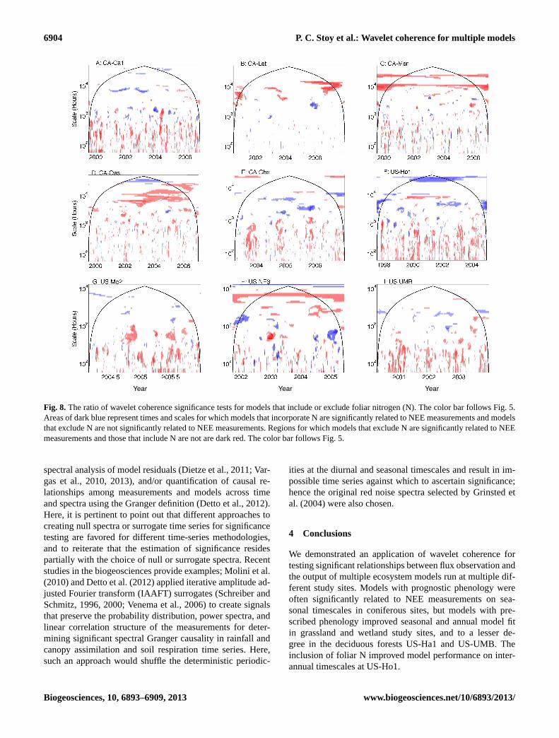
Models utilizing measurements of foliar N show improvedfits on interannual timescales compared models that excludeN at a coniferous forest (US-Ho1; Fig.8f) and to a lesserdegree at a deciduous forest (CA-Oas, Fig.8d). This findingsupports the incorporation of canopy N as an important com-ponent for accurately modeling spatial and temporal patternsin NEE (Hollinger et al., 2009; Ollinger and Smith, 2005;

Ollinger et al., 2008). However, it is discouraging that incor-porating N improves interannual model fit for only a coupleof sites rather than for all sites; note for example the poor fitof models that include N on timescales shorter than the inter-annual timescale at Ca-Oas (Fig.8d). Climatic variables tendto be unrelated or weakly related to observed NEE on inter-annual timescales (Stoy et al., 2009), and variability in bio-logical drivers like canopy N is thought to be a principle con-trol over NEE variability on interannual timescales (Richard-son et al., 2007). The role of biological lags (e.g., growth andNPP lagging behind C uptake) tends to be poorly representedin the current generation of ecosystem models (Keenan etal., 2012), as are the dynamics of the non-structural carbo-hydrates that can contribute to such lags (Gough et al., 2009,2010; Richardson et al., 2013). Modeling the biological re-sponses to interannual climatic variability continues to be amajor research challenge (Richardson et al., 2007; Siqueiraet al., 2006), and it appears that modeling N improves mod-els of NEE, but only in certain instances. Including foliar Nimproves model fit on certain timescales for different sites;for example including N appears to improve models in CA-Let, CA-Oas and CA-Obs, during summer months in 2006.The summer of 2006 was at the time the second warmest on



! ! Year ! ! ! ! ! Year ! ! ! ! ! ! Year!

Fig. 6.The ratio of wavelet coherence significance tests for models with prognostic prescribed phenology for nine sites in the North AmericanCarbon Program Interim Synthesis. The color bar follows Fig. 5. Areas of dark blue represent times and scales for which models that useprognostic leaf area index (LAI) are significantly related to NEE measurements and those that use prescribed LAI are not significantly relatedto NEE measurements. Regions for which models that use prescribed LAI are significant and those that use prognostic LAI are not significantare shown as dark red. The color bar follows Fig.5.

record in Canada, but the role of N in improving modeledNEE during these conditions is difficult to interpret and maybe due to correct hydrological response regardless of the Nsubroutine in the models.

3.8 Data assimilation

Data assimilation for formally fusing observations and mod-els has gained increased attention in the biogeosciences (Di-etze et al., 2013; Hill et al., 2011; Rastetter et al., 2010;Raupach et al., 2005; Williams et al., 2005). LoTEC ap-plied a data assimilation procedure in the NACP modelingexercise, and output in many instances represented a strik-ing improvement against the aggregate output of other mod-els (Fig.9). Namely, LoTEC output is significantly relatedto NEE measurements across many timescales at the decid-uous forests CA-Oas and US-UMB. LoTEC also demon-

strated improved fit compared to other models at seasonaland/or annual timescales at the coniferous forests CA-Obsand US-Ho1 and the crop US-Ne1. LoTEC was not signif-icantly related to NEE measurements (and the average ofother models were) across most sites with the exception ofCA-Oas and US-UMB. Results suggest that the optimizedparameters computed in the LoTEC data assimilation proce-dure can improve fit across times and timescales, especiallyfor some of the ecosystems that exhibit pronounced seasonal-ity in canopy dynamics (i.e., some deciduous forests, and theagricultural ecosystem). Results also demonstrate that dataassimilation does not always result in significant relation-ships between measurements and models; there are many pe-riods, often timescales between a day and about a month anda half (103 h) and at interannual timescales, where LoTECis not significantly related to measurements. Such findingsdemonstrate the importance of model parameterization, and



! ! Year ! ! ! ! ! Year ! ! ! ! ! Year!

Fig. 7. The ratio of wavelet coherence significance tests for models with different calculations of the net ecosystem exchange (NEE). Thecolor bar follows Fig. 5. Areas of dark blue represent times and scales for which models that calculate NEE as gross primary productivity(GPP) minus ecosystem respiration (ER) are significantly related to NEE measurements and models that calculate NEE as net primaryproductivity (NPP) minus heterotrophic respiration (HR) are not significantly related to NEE measurements. Regions for which models thatcalculate NEE as NPP minus HR are significant and GPP minus ER are not significant are dark red. The color bar follows Fig.5.

also suggest that data assimilation should not take the placeof efforts to improve model structure.

3.9 The analysis of models at multiple timescales

We used wavelet coherence as a criterion formodel/measurement comparison in this study. Spectralanalyses can also be used to discriminate among modelsubroutines and inputs (Stoy et al., 2005) or demonstratemodel improvement (Williams et al., 2009), and it is forthese purposes that wavelet coherence may find the most ap-plication in the biogeosciences.Wang et al.(2011) recentlyused wavelet coherence to quantify patterns of CABLEmodel output (Kowalczyk et al., 2006) and demonstratedhow model refinements improved predictions of NEE, latentheat and sensible heat on multiple timescales, althoughobserved patterns in interannual variability in NEE remaineddifficult for CABLE to resolve. Wavelet coherence has also

been applied to identify model/measurement mismatchesresulting from phenological response to monsoon activity(Hong and Kim, 2011) and for detailed studies on thecontrols over carbon cycling in individual sites (van Gorselet al., 2013). We suggest that any comprehensive modeldiagnostic toolkit should explore model frequency response,and we demonstrate the application of wavelet coherenceas a model–measurement comparison technique that is alsovisually intuitive. It is important to note that a wavelet co-herence test for matches in patterns, rather than magnitudes,and by itself is an incomplete metric for model fidelity. Thepotential for wavelet coherence to identify regions of falsepositive coherence erroneously must be acknowledged wheninterpreting results (Maraun et al., 2007).

Future research efforts should compare wavelet-based ap-proaches with other time-series decomposition techniques,including singular systems analysis (Mahecha et al., 2010),



! ! Year ! ! ! ! ! Year ! ! ! ! ! Year!

Fig. 8. The ratio of wavelet coherence significance tests for models that include or exclude foliar nitrogen (N). The color bar follows Fig.5.Areas of dark blue represent times and scales for which models that incorporate N are significantly related to NEE measurements and modelsthat exclude N are not significantly related to NEE measurements. Regions for which models that exclude N are significantly related to NEEmeasurements and those that include N are not are dark red. The color bar follows Fig.5.

spectral analysis of model residuals (Dietze et al., 2011; Var-gas et al., 2010, 2013), and/or quantification of causal re-lationships among measurements and models across timeand spectra using the Granger definition (Detto et al., 2012).Here, it is pertinent to point out that different approaches tocreating null spectra or surrogate time series for significancetesting are favored for different time-series methodologies,and to reiterate that the estimation of significance residespartially with the choice of null or surrogate spectra. Recentstudies in the biogeosciences provide examples;Molini et al.(2010) andDetto et al.(2012) applied iterative amplitude ad-justed Fourier transform (IAAFT) surrogates (Schreiber andSchmitz, 1996, 2000; Venema et al., 2006) to create signalsthat preserve the probability distribution, power spectra, andlinear correlation structure of the measurements for deter-mining significant spectral Granger causality in rainfall andcanopy assimilation and soil respiration time series. Here,such an approach would shuffle the deterministic periodic-

ities at the diurnal and seasonal timescales and result in im-possible time series against which to ascertain significance;hence the original red noise spectra selected byGrinsted etal. (2004) were also chosen.

4 Conclusions

We demonstrated an application of wavelet coherence fortesting significant relationships between flux observation andthe output of multiple ecosystem models run at multiple dif-ferent study sites. Models with prognostic phenology wereoften significantly related to NEE measurements on sea-sonal timescales in coniferous sites, but models with pre-scribed phenology improved seasonal and annual model fitin grassland and wetland study sites, and to a lesser de-gree in the deciduous forests US-Ha1 and US-UMB. Theinclusion of foliar N improved model performance on inter-annual timescales at US-Ho1.



! ! Year ! ! ! ! ! Year ! ! ! ! ! Year!

Fig. 9. The ratio of wavelet coherence significance tests for the model using a data assimilation procedure (LoTEC) versus other modelsthat do not use data assimilation. The color bar follows Fig. 5. Periods and scales in time for which LoTEC is significantly related to NEEmeasurements and other models are not significantly related to NEE measurements (on average) are shown as dark blue. Regions for whichmodels other than LoTEC are significantly related to NEE measurements and LoTEC is not significantly related to NEE measurements areshown as dark red. The color bar follows Fig.5.

Model pattern tended to match observed NEE on diur-nal timescales during the growing season and on annualtimescales (e.g., Figs. 1 and 2), but previous analyses indi-cate that models often misrepresent the magnitude of fluxeson these highly energetic timescales (Dietze et al., 2011). De-spite correct frequency responses on growing-season diurnaland annual timescales as we find here,Dietze et al.(2011)demonstrated that proper parameterization of flux magnitudeon these scales should remain a focus of modeling efforts.LoTEC results (Figs.3 and9) hint that data assimilation canimprove model fit on the intermediate weekly to seasonaltimescales during many periods, but modeled flux variabil-ity on diurnal and interannual timescales was often not sig-nificantly related to measurements, suggesting that modelsstill require mechanistic improvements even under parametersets optimized by the data assimilation routine. Mechanisticexplanations for describing interannual NEE variability still

elude most models, although correctly modeling N dynamicsmay be a strategy for progressing on this problem in someecosystems (Fig.8).

Wavelet coherence adds an additional diagnostic tool toa modeler’s conceptual toolbox for evaluating the perfor-mance of single models or suites of models (Grinsted et al.,2004; Torrence and Compo, 1998; Williams et al., 2009). Fu-ture efforts should determine the benefits and drawbacks ofwavelet, Fourier, and singular systems analysis approachesfor model/measurement comparisons (Katul et al., 2001; Ma-hecha et al., 2010; Siqueira et al., 2006; Maraun et al., 2007;Vargas et al., 2010), use the outcomes of multiple spectralanalyses to provide insight into how and why models fail,and use this information to improve model performance atthe multiple times and timescales at which biogeochemicalfluxes vary.



Acknowledgements.First and foremost, we wish to thank all ofthe researchers involved in eddy covariance data collection andcuration, and in model development and testing. P. C. Stoy thanksMatteo Detto and Aslak Grinsted for helpful discussions and codeexamples regarding wavelet coherence and the National ScienceFoundation (Scaling ecosystem function: Novel Approaches fromMaxEnt and Multiresolution, DBI #1021095). We would like tothank the North American Carbon Program Site-Level InterimSynthesis team, the Modeling and Synthesis Thematic DataCenter, and the Oak Ridge National Laboratory Distributed ActiveArchive Center, and Larry Flanagan for collecting, organizing, anddistributing the model output and flux observations required for thisanalysis. We also thank Robert Bemis for creating the MATLABcode that followed the suggestions ofLight and Bartlein(2004) forimproved use of color in images. This study was in part supportedby the US National Aeronautics and Space Administration (NASA)grant NNX06AE65G, the US National Oceanic and AtmosphericAdministration (NOAA) grant NA07OAR4310115, and the USNational Science Foundation (NSF) grant OPP-0352957 to theUniversity of Colorado at Boulder. This study was part of the NorthAmerican Carbon Program.

Edited by: M. Bahn

References

Akaike, H.: A new look at the statistical model identification, IEEET. Automat. Contr., 19, 716–723, 1974.

Arain, M. A., Yaun, F., and Black, T. A.: Soil-plant nitrogen cyclingmodulated carbon exchanges in a western temperate conifer for-est in Canada, Agr. Forest Meteorol., 140, 171–192, 2006.

Baker, I. T., Prihodko, L., Denning, A. S., Goulden, M., Miller, S.,and da Rocha, H. R.: Seasonal drought stress in the Amazon:Reconciling models and observations, J. Geophys. Res., 113,G00B01, doi:10.1029/2007JG000644, 2008.

Barr, A. G., Hollinger, D. Y., Richardson, A. D.: CO2 flux measure-ment uncertainty estimates for NACP, Eos Trans. AGU, 90, FallMeet. Suppl., Abstract B54A-04.

Bauerle, W. L., Oren, R., Way, D. A, Qian, S. S., Stoy, P.C., Thornton, P. E., Bowden, J. D., Hoffman, F. M., andReynolds, R. F.: Photoperiodic regulation of the seasonalpattern of photosynthetic capacity and the implications forcarbon cycling, P. Natl. Acad. Sci. USA, 109, 8612–8617.doi:10.1073/pnas.1119131109, 2012.

Causarano, H. J., Shaw, J. M., Franzluebbers, A. J., Reeves, D. W.,Raper, R. L., Balkcom, K. S., Norfleet, M. L., and Izaurralde,R. C.: Simulating field-scale soil organic carbon dynamics usingEPIC, Soil Sci. Soc. Am. J., 71, 1174–1185, 2007.

Detto, M., Molini, A., Katul, G. G., Stoy, P. C., Palmroth, S., andBaldocchi, D. D.: Causality and persistence in ecological sys-tems: a nonparametric spectral Granger causality approach, Am.Nat., 179, 524–535, 2012.

Dietze, M. C, Vargas, R., Richardson, A. D., Stoy, P. C., Barr,A. G., Anderson, R. S., Arain, A., Baker, I. T., Black, T. A.,Chen, J. M., Ciais, P., Flanagan, L. B., Gough, C. M., Grant,R. F., Hollinger, D. Y., Izaurralde, C., Kucharik, C. J., Lafleur,P. M., Liu, S., Lokupitiya, E., Luo, Y., Munger, J. W., Peng,C., Poulter, B., Price, D. T., Ricciuto, D. M., Riley, W. J., Sa-hoo, A. K., Schaefer, K., Tian, H., Verbeeck, H., and Verma, S.

B.: Characterizing the performance of ecosystem models acrosstime scales: A spectral analysis of the North American CarbonProgram site-level synthesis, J. Geophys. Res., 116, G04029,doi:10.1029/2011JG001661, 2011.

Dietze, M. C., LeBauer, D. S., and Kooper, R.: On improving thecommunication between models and data, Plant Cell Environ.,36, 1575–1585, doi:10.1111/pce.12043, 2013.

Fisher, J. I., Richardson, A. D., and Mustard, J. F.: Phenologymodel from surface meteorology does not capture satellite-based greenup estimations, Glob. Change Biol., 13, 707–721,doi:10.1111/j.1365-2486.2006.01311.x, 2007.

Flanagan, L. B., Wever, L. A., and Carlson, P. J.: Seasonal and inter-annual variation in carbon dioxide exchange and carbon balancein a northern temperate grassland, Glob. Change Biol., 8, 599–615, 2002.

Friedlingstein, P., Cox, P., Betts, R. A., Bopp, L., von Blow, W.,Brovkin, V., Cadule, P., Doney, S. C., Eby, M., Fung, I. Y., Bala,G., John, J., Jones, C. D., Joos, F., Kato, T., Kawamiya, M.,Knorr, W., Lindsay, K., Matthews, H. D., Raddatz, T., Rayner, P.J., Reick, C., Roeckner, E., Schnitzler, K.-G., Schnur, R., Strass-mann, K., Weaver, A. J., Yoshikawa, C., and Zeng, N.: Climate-carbon cycle feedback analysis: results from the C4MIP modelintercomparison, J. Climate, 19, 3337–3353, 2006.

Gough, C. M., Vogel, C. S., Schmid, H. P., Su, H.-B., and Curtis,P. S.: Multi-year convergence of biometric and meteorologicalestimates of forest carbon storage, Agr. Forest Meteorol., 148,158–170, 2008.

Gough, C. M., Flower, C. E., Vogel, C. S., Dragoni, D., and Curtis,P. S.: Whole-ecosystem labile carbon production in a north tem-perate deciduous forest, Agr. Forest Meteorol., 149, 1531–1540,2009.

Gough, C. M., Flower, C. E., Vogel, C. S., and Curtis, P. S.: Pheno-logical and temperature controls on the temporal non-structuralcarbohydrate dynamics ofPopulus grandidentataand Quercusrubra, Forests, 1, 65–81, 2010.

Grant, R. F., Arain, A., Arora, V., Barr, A., Black, T. A., Chen, J.,Wang, S., Yuan, F., and Zhang, Y.: Intercomparison of techniquesto model high temperature effects on CO2 and energy exchangein temperate and boreal coniferous forests, Ecol. Model., 188,217–252, 2005.

Gray, J.: Jim Gray on eScience: A transformed scientific method, in:The fourth paradigm: Data-intensive scientific discovery, editedby: Hey, T., Tansley, S., and Tolle, K., Microsoft Research, 284,2009.

Griffis, T. J., Black, T. A., Morgenstern, K., Barr, A. G., Nesic, Z.,Drewitt, G. B., Guamont-Guay, D., and McCaughey, J. H.: Eco-physiological controls on the carbon balances of three southernboreal forests, Agr. Forest Meteorol., 117, 53–71, 2003.

Grinsted, A., Moore, J. C., and Jevrejeva, S.: Application of thecross wavelet transform and wavelet coherence to geophysicaltime series, Nonlinear Proc. Geoph., 11, 561–566, 2004.

Hanson, P. J., Amthor, J. S., Wullschleger, S. D., Wilson, K. F.,Grant, R. F., Hartley, A., Hui, D. F., Hunt, E. R. J., Johnson,D. W., Kimball, J. S., King, A. W., Y., L., McNulty, S. G.,Sun, G., Thornton, P. E., S., W., Williams, M., Baldocchi, D.D., and Cushman, R. M.: Oak forest carbon and water simula-tions: model intercomparisons and evaluations against indepen-dent data., Ecol. Monogr., 74, 443–489, 2004.


http://dx.doi.org/10.1029/2007JG000644

http://dx.doi.org/10.1073/pnas.1119131109

http://dx.doi.org/10.1029/2011JG001661

http://dx.doi.org/10.1111/pce.12043

http://dx.doi.org/10.1111/j.1365-2486.2006.01311.x


Hill, T. C., Quaife, T., and Williams, M.: A data assimila-tion method for using low-resolution Earth observation datain heterogeneous ecosystems, J. Geophys. Res., 116, D08117,doi:10.1029/2010jd015268, 2011.

Hollinger, D. Y., Ollinger, S. V., Richardson, A. D., Meyers, T.,Dail, D. B., Martin, M. E., Scott, N. A., Arkebauer, T. J., Bal-docchi, D. D., Clark, K. L., Curtis, P. S., Davis, K. J., Desai, A.R., Dragoni, D., Goulden, M. L., Gu, L., Katul, G. G., Pallardy,S. G., Paw U, K. T., Schmid, H. P., Stoy, P. C., Suyker, A. E., andVerma, S. B.: Albedo estimates for land surface models and sup-port for a new paradigm based on foliage nitrogen concentration.,Glob. Change Biol., 16, 696–710, 2009.

Hong, J. and Kim, J.: Impact of the Asian monsoon climate onecosystem carbon and water exchanges: a wavelet analysis andits ecosystem modeling implications, Glob. Change Biol., 17,1900–1916, 2011.

Katul, G. G., Lai, C.-T., Schäfer, K. V. R., Vidakovic, B., Albertson,J. D., Ellsworth, D. S., and Oren, R.: Multiscale analysis of vege-tation surface fluxes: from seconds to years, Adv. Water Resour.,24, 1119–1132, 2001.

Keenan, T. F., Baker, I., Barr, A., Ciais, P., Davis, K., Dietze, M.,Dragoni, D., Gough, C. M., Grant, R., Hollinger, D., Hufkens,K., Poulter, B., McCaughey, H., Raczka, B., Ryu, Y., Schaefer,K., Tian, H., Verbeeck, H., Zhao, M., and Richardson, A. D.:Terrestrial biosphere model performance for inter-annual vari-ability of land-atmosphere CO2 exchange, Glob. Change Biol.,18, 1971–1987, 2012.

Kowalczyk, E. A., Wang, Y. P., Law, R. M., Davies, H. L., Mc-Gregor, J. L., and Abramowitz, G.: The CSIRO atmosphere bio-sphere land exchange (CABLE) model for use in climate modelsand as an offline model, CSIRO Marine and Atmospheric Re-search, ISBN 1 921232 39 0, 2006.

Krinner, G., Viovy, N., de Noblet-Ducoudré, N., Ogée, J., Polcher,J., Friedlingstein, P., Ciais, P., Sitch, S., and Prentice, I. C.:A dynamic global vegetation model for studies of the cou-pled atmosphere-biosphere system, Global Biogeochem. Cy., 19,GB1015, doi:10.1029/2003GB002199, 2005.

Krishnan, P., Black, T. A., Grant, N. J., Barr, A. G., Hogg, E. H.,Jassal, R. S., Morgenstern, K.: Impact of changing soil moisturedistribution on net ecosystem productivity of a boreal aspen for-est during and following drought, Agr. For. Meteorol. 139, 208–223, 2006.

Kucharik, C. J. and Twine, T. E.: Residue, respiration and residuals:Evaluation of a dynamic agroecosystem model using eddy fluxmeasurements and biometric data, Agr. Forest Meteorol., 146,134–158, 2007.

Lafleur, P. M., Roulet, N. T., Bubier, J. L., Moore, T. R., and Frolk-ing, S.: Interannual variability in the peatland-atmosphere carbondioxide exchange at an ombrotrophic bog, Global Biogeochem.Cy., 17, 1036, doi:10.1029/2002GB001983, 2003.

Law, B. E., Arkebauer, T. J., Campbell, J. L., Chen, J., Sun, O.,Schwartz, M., van Ingen, C., and Verma, S.: Terrestrial carbonobservations: Protocols for vegetation sampling and data submis-sion, Report 55, FAO, Rome, 87, 2008.

Li, H., Qiu, J., Wang, L., Tang, H., Li, C., and Van Ranst, E.: Mod-elling impacts of alternative farming management practices ongreenhouse gas emissions from a winter wheat-maize rotationsystem in China, Agr. Ecosyst. Environ., 135, 24–33, 2010.

Light, A. and Bartlein, P. J.: The end of the rainbow? Color schemesfor improved data graphics, Eos Trans. AGU, 85, 385–391, 2004.

Liu, J., Chen, J. M., Cihlar, J., and Chen, W.: Net primary produc-tivity distribution in the BOREAS region from a process modelusing satellite and surface data, J. Geophys. Res., 104, 27735–27754, 1999.

Lokupitiya, E., Denning, S., Paustian, K., Baker, I., Schaefer, K.,Verma, S., Meyers, T., Bernacchi, C. J., Suyker, A., and Fischer,M.: Incorporation of crop phenology in Simple Biosphere Model(SiBcrop) to improve land-atmosphere carbon exchanges fromcroplands, Biogeosciences, 6, 969–986, doi:10.5194/bg-6-969-2009, 2009.

Mahecha, M. D., Reichstein, M., Jung, M., Senevirante, S. I., Za-ehle, S., Beer, C., Braakhekke, M. C., Carvalhais, N., Lange,H., Le Maire, G., and Moors, E.: Comparing observationsand process-based simulations of biosphere-atmosphere ex-changes on multiple timescales, J. Geophys. Res., 115, G02003,doi:10.1029/2009JG001016, 2010.

Maraun, D. and Kurths, J.: Cross wavelet analysis: significance test-ing and pitfalls, Nonlinear Proc. Geoph., 11, 505–514, 2004.

Maraun, D., Kurths, J., and Holschneider, M.: Nonstationary Gaus-sian processes in wavelet domain: Synthesis, estimation, and sig-nificance testing, Physical Review E, 75, 16707, 2007.

Medvigy, D., Wofsy, S. C., Munger, J. W., Hollinger, D. Y.,and Moorcroft, P. R.: Mechanistic scaling of ecosystem func-tion and dynamics in space and time: Ecosystem Demo-raphy model version 2, J. Geophys. Res., 114, G01002,doi:10.1029/2008JG000812, 2009.

Molini, A., Katul, G. G., and Porporato, A.: Causality across rainfalltime scales revealed by continuous wavelet transforms, JournalGeophys. Res., 115, D14123, doi:10.1029/2009JD013016, 2010.

Ollinger, S. V. and Smith, M.-L.: Net primary production andcanopy nitrogen in a temperate forest landscape: an analysis us-ing imaging spectroscopy, modeling and field data, Ecosystems,8, 760–778, 2005.

Ollinger, S. V., Richardson, A. D., Martin, M. E., Hollinger, D. Y.,Frolking, S., Reich, P. B., Plourde, L. C., Katul, G. G., Munger,J. W., Oren, R., Smith, M.-L., Paw U, K. T., Bolstad, P. V., Cook,B. D., Day, M. C., Martin, T. A., Monson, R. K., and Schmid,H. P.: Canopy nitrogen, carbon assimilation, and albedo in tem-perate and boreal forests: functional relations and potential cli-mate feedbacks, P. Natl. Acad. Sci. USA, 105, 19336–19341,doi:10.1073/pnas.0810021105, 2008.

Papale, D., Reichstein, M., Aubinet, M., Canfora, E., Bernhofer, C.,Kutsch, W., Longdoz, B., Rambal, S., Valentini, R., Vesala, T.,and Yakir, D.: Towards a standardized processing of Net Ecosys-tem Exchange measured with eddy covariance technique: algo-rithms and uncertainty estimation, Biogeosciences, 3, 571–583,doi:10.5194/bg-3-571-2006, 2006.

Rastetter, E. B., Williams, M., Griffin, K. L., Kwiatkowski, B.L., Tomasky, G., Potosnak, M. J., Stoy, P. C., Shaver, G. R.,Stieglitz, M., Hobbie, J. E., and Kling, G. W.: Processing arcticeddy-flux data using a simple carbon-exchange model embed-ded in the ensemble Kalman filter, Ecol. Appl., 20, 1285–1301,doi:10.1890/09-0876.1, 2010.

Raupach, M. R., Rayner, P. J., Barrett, D. J., DeFries, R. S.,Heimann, M., Ojima, D., Quegan, S., and Schmullius, C. C.:Model-data synthesis in terrestrial carbon observation: meth-


http://dx.doi.org/10.1029/2010jd015268

http://dx.doi.org/10.1029/2003GB002199

http://dx.doi.org/10.1029/2002GB001983

http://dx.doi.org/10.5194/bg-6-969-2009

http://dx.doi.org/10.5194/bg-6-969-2009

http://dx.doi.org/10.1029/2009JG001016

http://dx.doi.org/10.1029/2008JG000812

http://dx.doi.org/10.1029/2009JD013016

http://dx.doi.org/10.1073/pnas.0810021105

http://dx.doi.org/10.5194/bg-3-571-2006

http://dx.doi.org/10.1890/09-0876.1


ods, data requirements and data uncertainty specifications, Glob.Change Biol., 11, 378–397, 2005.

Reed, B. C., Brown, J. F., VanderZee, D., Loveland, T. R.,Merchant, J. W., and Ohlen, D. O.: Measuring phenologicalvariability from satellite imagery, J. Veg. Sci., 5, 703–714,doi:10.2307/3235884, 1994.

Reichstein, M., Falge, E., Baldocchi, D., Papale, D., Aubinet,M., Berbigier, P., Bernhofer, C., Buchmann, N., Gilmanov, T.G., Granier, A., Grünwald, T., Havránková, K., Ilvesniemi, H.,Janous, D., Knohl, A., Laurila, T., Lohila, A., Loustau, D., Mat-teucci, G., Meyers, T., Miglietta, F., Ourcival, J.-M., Pumpanen,J., Rambal, S., Rotenberg, E., Sanz, M., Tenhunen, J., Seufert, G.,Vaccari, F., Vesala, T., Yakier, D., and Valentini, R.: On the sep-aration of net ecosystem exchange into assimilation and ecosys-tem respiration: Review and improved algorithm, Glob. ChangeBiol., 11, 1424–1439, 2005.

Ricciuto, D. M., Thornton, P. E., Schaefer, K., Cook, R. B., andDavis, K. J.: How uncertainty in gap-filled meteorological inputforcing at eddy covariance towers impacts modeled carbon andenergy flux, Eos Trans. AGU, 90, Fall Meet. Suppl., AbstractB54A-03, 2009.

Richardson, A. D., Hollinger, D. Y., Aber, J. D., Ollinger, S. V., andBraswell, B. H.: Environmental variation is directly responsiblefor short- but not long-term variation in forest-atmosphere carbonexchange, Glob. Change Biol., 13, 788–803, 2007.

Richardson, A. D., Mahecha, M. D., Falge, E., Kattge, J., Moffat,A. M., Papale, D., Reichstein, M., Stauch, V. J., Braswell, B. H.,Churkina, G., Kruijt, B., and Hollinger, D. Y.: Statistical proper-ties of random CO2 flux measurement uncertainty inferred frommodel residuals, Agr. Forest Meteorol., 148, 38–50, 2008.

Richardson, A. D., Hollinger, D. Y., Dail, D. B., Lee, J. T., Munger,J. W., and O’Keefe, J.: Influence of spring phenology on sea-sonal and annual carbon balance in two contrasting New Englandforests, Tree Physiol., 29, 321–331, 2009.

Richardson, A. D., Anderson, R. S., Arain, M. A., Barr, A. G.,Bohrer, G., Chen, G., Chen, J. M., Ciais, P., Davis, K. J., De-sai, A. R., Dietze, M. C., Dragoni, D., Garrity, S. R., Gough, C.M., Grant, R., Hollinger, D. Y., Margolis, H. A., McCaughey,H., Migliavacca, M., Monson, R. K., Munger, J. W., Poulter, B.,Raczka, B. M., Ricciuto, D. M., Sahoo, A. K., Schaefer, K., Tian,H., Vargas, R., Verbeeck, H., Xiao, J., and Xue, Y.: Terrestrialbiosphere models need better representation of vegetation phe-nology: results from the North American Carbon Program SiteSynthesis, Glob. Change Biol., 18, 566–584, doi:10.1111/j.1365-2486.2011.02562.x, 2012.

Richardson, A. D., Carbone, M. S., Keenan, T. F. , Czimczik, C.I., Hollinger, D. Y., Murakami, P., Schaberg, P. G., and Xu, X.:Seasonal dynamics and age of stemwood nonstructural carbo-hydrates in temperate forest trees, New Phytol., 197, 850–861,doi:10.1111/nph.12042, 2013.

Riley, W. J., Still, C. J., Torn, M. S., and Berry, J. A.: A mechanisticmodel of H2

18O and C18OO fluxes between ecosystems and theatmosphere: Model description and sensitivity analyses, GlobalBiogeochem. Cy., 16, 1095, doi:10.1029/2002GB001878, 2002.

Schaefer, K., Zhang, T., Slater, A. G., Lu, L., Etringer,A., and Baker, I.: Improving simulated soil temperaturesand soil freeze/thaw at high-latitude regions in the SimpleBiosphere/Carnegie-Ames-Stanford Approach model, J. Geo-phys. Res., 114, F02021, doi:10.1029/2008JF001125, 2009.

Schaefer, K., Schwalm, C. R., Williams, C., Arain, M. A., Barr, A.,Chen, J. M., Davis, K. J., Dimitrov, D., Hilton, T. W., Hollinger,D. Y., Humphreys, E., Poulter, B., Raczka, B. M., Richardson,A. D., Sahoo, A., Thornton, P., Vargas, R., Verbeeck, H., An-derson, R., Baker, I., Black, T. A., Bolstad, P., Chen, J., Cur-tis, P. S., Desai, A. R., Dietze, M., Dragoni, D., Gough, C.,Grant, R. F., Gu, L., Jain, A., Kucharik, C., Law, B., Liu, S.,Lokipitiya, E., Margolis, H. A., Matamala, R., McCaughey, J.H., Monson, R., Munger, J. W., Oechel, W., Peng, C., Price, D.T., Ricciuto, D., Riley, W. J., Roulet, N., Tian, H., Tonitto, C.,Torn, M., Weng, E., and Zhou, X.: A model-data comparisonof gross primary productivity: Results from the North AmericanCarbon Program site synthesis, J. Geophys. Res., 117, G03010,doi:10.1029/2012jg001960, 2012.

Schmid, H. P., Su, H. B., Vogel, C. S., and Curtis, P. S.: Ecosystem-atmosphere exchange of carbon dioxide over a mixed hardwoodforest in northern lower Michigan, J. Geophys. Res.-Atmos., 108,4417, doi:10.1029/2002JD003011, 2003.

Schreiber, T. and Schmitz, A.: Improved surrogate data for nonlin-earity tests, Phys. Rev. Lett., 77, 635–638, 1996.

Schreiber, T. and Schmitz, A.: Surrogate time series, Physica D,142, 346–382, 2000.

Schwalm, C. R., Black, T. A., Morgenstern, K., and Humphreys, E.R.: A method for deriving net primary productivity and compo-nent respiratory fluxes from tower-based eddy covariance data:a case study using a 17-year data record from a Douglas-firchronosequence, Glob. Change Biol., 13, 370–385, 2007.

Schwalm, C. R., Williams, C. A., Schaefer, K., Anderson, R., Arain,M. A., Baker, I., Barr, A. G., Black, T. A., Chen, G., Chen, J.M., Ciais, P., Davis, K. J., Desai, A. R., Dietze, M., Dragoni,D., Fischer, M. L., Flanagan, L. B., Grant, R., Gu, L., Hollinger,D., Izaurralde, R. C., Kucharik, C. J., Lafleur, P. M., Law, B. E.,Li, L., Li, Z., Liu, S., Lokupitiya, E., Luo, Y., Ma, S., Margolis,H., Matamala, R., McCaughey, J. H., Monson, R. K., Oechel,W., Peng, C., Poulter, B., Price, D. T., Riciutto, D. M., Riley,W., Sahoo, A. K., Sprintsin, M., Sun, J., Tian, H., Tonitto, C.,Verbeeck, H., and Verma, S. B.: A model-data intercomparisonof CO2 exchange across North America: Results from the NorthAmerican Carbon Program Site Synthesis, J. Geophys. Res, 115,G00H05, doi:10.1029/2009JG001229, 2010.

Siqueira, M. B. S., Katul, G. G., Sampson, D. A., Stoy, P. C.,Juang, J.-Y., McCarthy, H. R., and Oren, R.: Multi-scale modelinter-comparisons of CO2 and H2O exchange rates in a matur-ing southeastern U.S. pine forest, Glob. Change Biol., 12, 1189–1207, 2006.

Sitch, S., Smith, B., Prentice, I. C., Arneth, A., Bondeau, A.,Cramer, W., Kaplan, J. O., Levis, S., Lucht, W., Sykes, M., Thon-icke, K., and Venevsky, S.: Evaluation of ecosystem dynamics,plant geography and terrestrial carbon cycling in the LPJ dy-namic global vegetation model, Glob. Change Biol., 9, 161–185,2003.

Stoy, P. C., Katul, G. G., Siqueira, M. B. S., Juang, J.-Y., McCarthy,H. R., Kim, H.-S., Oishi, A. C., and Oren, R.: Variability innet ecosystem exchange from hourly to inter-annual time scalesat adjacent pine and hardwood forests: a wavelet analysis, TreePhysiol., 25, 887–902, 2005.

Stoy, P. C., Katul, G. G., Siqueira, M. B. S., Juang, J.-Y., Novick, K.A., Uebelherr, J. M. and Oren, R.: An evaluation of models forpartitioning eddy covariance-measured net ecosystem exchange


http://dx.doi.org/10.2307/3235884

http://dx.doi.org/10.1111/j.1365-2486.2011.02562.x

http://dx.doi.org/10.1111/j.1365-2486.2011.02562.x

http://dx.doi.org/10.1111/nph.12042

http://dx.doi.org/10.1029/2002GB001878

http://dx.doi.org/10.1029/2008JF001125

http://dx.doi.org/10.1029/2012jg001960

http://dx.doi.org/10.1029/2002JD003011

http://dx.doi.org/10.1029/2009JG001229


into photosynthesis and respiration, Agr. Forest Meteorol., 141,2–18, doi:10.1016/j.agrformet.2006.09.001, 2006.

Stoy, P. C., Richardson, A. D., Baldocchi, D. D., Katul, G. G.,Stanovick, J., Mahecha, M. D., Reichstein, M., Detto, M., Law,B. E., Wohlfahrt, G., Arriga, N., Campos, J., McCaughey, J.H., Montagnani, L., Paw U, K. T., Sevanto, S., and Williams,M.: Biosphere-atmosphere exchange of CO2 in relation to cli-mate: a cross-biome analysis across multiple time scales, Bio-geosciences, 6, 2297–2312, doi:10.5194/bg-6-2297-2009, 2009.

Sus, O., Williams, M., Bernhofer, C., Béziat, P., Buchmann, N.,Ceschia, E., Doherty, R., Eugster, W., Grünwald, T., Kutsch, W.,Smith, P., and Wattenbach, M.: A linked carbon cycle and cropdevelopmental model: Description and evaluation against mea-surements of carbon fluxes and carbon stocks at several Europeanagricultural sites, Agr. Ecosyst. Environ., 139, 402–418, 2010.

Taylor, K. E.: Summarizing multiple aspects of model performancein a single diagram, J. Geophys. Res, 106, 7183–7192, 2001.

Thomas, C. K., Law, B. E., Irvine, J., Martin, J. G., Pettijohn, J.C., and Davis, K. J.: Seasonal hydrology explains interannualand seasonal variation in carbon and water exchange in a semi-arid mature ponderosa pine forest in central Oregon, J. Geophys.Res., 114, G04006, doi:10.1029/2009JG001010, 2009.

Thornton, P. E., Running, S. W., and Hunt, E. R.: Biome-BGC:Terrestrial Ecosystem Processes Model, Version 4.1.1, OakRidge National Laboratory Distributed Active Archive Center,doi:10.3334/ORNLDAAC/805, 2005.

Tian, H. Q., Chen, G., Liu, M., Zhang, C., Sun, G., Lu, C., Xu, X.,Ren, W., Pan, P., and Chappelka, A.: Model estimates of ecosys-tem net primary productivity, evapotranspiration and water useefficiency in the Southern United States during 1895–2007, For-est Ecol. Manag., 259, 1311–1327, 2010.

Torrence, C. and Compo, G. P.: A practical guide to wavelet analy-sis, B. Am. Meteorol. Soc., 79, 61–78, 1998.

Torrence, C. and Webster, P.: Interdecadal changes in the ENSO-Monsoon system, J. Climate, 12, 2679–2690, 1999.

Urbanski, S. P., Barford, C., Wofsy, S., Kucharik, C. J., Pyle, E. H.,Budney, J., McKain, K., Fitzjarrald, D., Czikowsky, M. J., andMunger, J. W.: Factors controlling CO2 exchange on timescalesfrom hourly to decadal at Harvard Forest, J. Geophys. Res., 112,G02020, doi:10.1029/2006JG000293, 2007.

Van Gorsel, E., Berni, J. A. J., Briggs, P., Cabello-Leblic, A.,Chasmer, L., Cleugh, H. A., Hacker, J., Hantson, S., Haverd,V., Hughes, D., Hopkinson, C., Keith, H., Kljun, N., Leun-ing, R., Yebra, M., and Zegelin, S.: Primary and secondaryeffects of climate variability on net ecosystem carbon ex-change in an evergreen Eucalyptus forest, Agr. Forest Meteorol.,doi:10.1016/j.agrformet.2013.04.027, 2013.

Vargas, R., Detto, M., Baldocchi, D. D., and Allen, M. F.: Multi-scale analysis of temporal variability of soil CO2 production asinfluenced by weather and vegetation, Glob. Change Biol., 16,1589–1605, doi:10.1111/j.1365-2486.2009.02111.x, 2010.

Vargas, R., Sonnentag, O., Abramowitz, G., Carrara, A., Chen, J.M., Ciais, P., Correira, A., Keenan, T., Kobayashi, H., Ourci-val, J–M., Papale, D., Pearson, D., Pereira, J. S., Piao, S. L.,Rambal, S., and Baldocchi, D. D.: Drought influences the accu-racy of simulated ecosystem fluxes: a model–data meta–analysisfor Mediterranean oak woodlands, Ecosystems, 16, 749–764,doi:10.1007/s10021-013-9648-1, 2013.

Venema, V., Ament, F., and Simmer, C.: A stochastic iterative am-plitude adjusted Fourier transform algorithm with improved ac-curacy, Nonlinear Proc. Geoph., 13, 321–328, 2006.

Verma, S. B., Dobermann, A., and Cassman, K. G.: Annual carbondioxide exchange in irrigated and rainfed maize-based agroe-cosystems, Agr. Forest Meteorol., 131, 77–96, 2005.

Wang, W., Dungan, J., Hashimoto, H., Michaelis, A. R., Milesi,C., Ichii, K., and Nemani, R. R.: Diagnosing and assessing un-certainties of terrestrial ecosystem models in a multi-model en-semble experiment: 2. Carbon balance, Glob. Change Biol., 17,1367–1378, doi:10.1111/j.1365-2486.2010.02315.x, 2010.

Wang, Y. P., Kowalczyk, E. A., Leuning, R., Abramowitz, G.,Raupach, M., Pak, B. C., van Gorsel, E., and Luhar, A.:Diagnosing errors in a land surface model (CABLE) in thetime and frequency domains, J. Geophys. Res., 116, G01034,doi:10.1029/2010JG001385, 2011.

Weng, E. and Luo, Y.: Soil hydrological properties regu-late grassland ecosystem responses to multifactor globalchange: A modeling analysis, J. Geophys. Res., 113, G03003,doi:10.1029/2007JG000539, 2008.

Williams, M., Schwarz, P. A., Law, B., Irvine, J., and Kurpius, M.R.: An improved analysis of forest carbon dynamics using dataassimilation, Glob. Change Biol., 11, 89–105, 2005.

Williams, M., Richardson, A. D., Reichstein, M., Stoy, P. C.,Peylin, P., Verbeeck, H., Carvalhais, N., Jung, M., Hollinger,D. Y., Kattge, J., Leuning, R., Luo, Y., Tomelleri, E.,Trudinger, C. M., and Wang, Y. -P.: Improving land surfacemodels with FLUXNET data, Biogeosciences, 6, 1341–1359,doi:10.5194/bg-6-1341-2009, 2009.

Williamson, T. B., Price, D. T., Beverley, J. L., Bothwell, P. M.,Frenkel, B., Park, J., and Patriquin, M. N.: Assessing potentialbiophysical and socioeconomic impacts of climate change onforest-based communities: a methodological case study, NaturalResources Canada, Canadian Forest Service, Edmonton, ABInf.Rep. NOR-X-415E, 2008.

Zhan, X. W., Xue, Y. K., and Collatz, G. J.: An analytical approachfor estimating CO2 and heat fluxes over the Amazonian region,Ecol. Model., 162, 97–117, 2003.

Zhou, X. L., Peng, C. H., Dang, Q. L., Sun, J. F., Wu, H. B.,and Hua, D.: Simulating carbon exchange in Canadian borealforests I: model structure, validation, and sensitivity analysis,Ecol. Model., 219, 287–299, 2008.


http://dx.doi.org/10.1016/j.agrformet.2006.09.001

http://dx.doi.org/10.5194/bg-6-2297-2009

http://dx.doi.org/10.1029/2009JG001010

http://dx.doi.org/10.3334/ORNLDAAC/805

http://dx.doi.org/10.1029/2006JG000293

http://dx.doi.org/10.1016/j.agrformet.2013.04.027

http://dx.doi.org/10.1111/j.1365-2486.2009.02111.x

http://dx.doi.org/10.1007/s10021-013-9648-1

http://dx.doi.org/10.1111/j.1365-2486.2010.02315.x

http://dx.doi.org/10.1029/2010JG001385

http://dx.doi.org/10.1029/2007JG000539

http://dx.doi.org/10.5194/bg-6-1341-2009

biogeosciences evaluating the agreement between …faculty.geog.utoronto.ca/chen/chen's...

Documents