biogeography and speciation of southwestern australian frogs · biogeography and speciation of a...
TRANSCRIPT

1
Biogeography andspeciation of
southwestern Australianfrogs
Danielle L. EdwardsB. Env. Sc. (Hons)
Supervisor: Prof. J. Dale Roberts
This thesis is presented for the degree of Doctor of Philosophy of The University ofWestern Australia, School of Animal Biology
2007

2

3
Thesis Declaration
This thesis contains published work and work prepared for publication, some of whichhas been co-authored. The bibliographic details of the works and where they appear inthe thesis are set out below.
Edwards, DL. Biogeography and speciation of a direct developing frog from thecoastal arid zone of Western Australia. In Review with Molecular Phylogenetics andEvolution. (Data Chapter 1).
Edwards, DL, Roberts, JD and Keogh, SK (In Press). Impact of Plio-Pleistocene aridcycling on the population history of a southwestern Australian frog. Molecular Ecology.(Data Chapter 2).
(This work was primarily conducted by DLE (~90%), JDR provided assistance with projectdesign, and editing and advice on field collection (~5%), JSK provided access to his molecularlab, assistance with editing and advice on analysis techniques (~5%)).
Edwards, DL, Roberts, JD and Keogh, SK. Climatic fluctuations shape thephylogeography of a mesic adapted direct developing frog from the southwesternAustralian biodiversity hotpot. In Prep for Journal of Biogeography. (Data Chapter 3).
(This work was primarily conducted by DLE (~90%), JDR provided assistance with projectdesign, and editing and advice on field collection (~5%), JSK provided access to his molecularlab, assistance with editing and advice on analysis techniques (~5%)).
The fourth data chapter is also to be published; the manuscript is still in preparation.
Signatures…………………………………………………………………………………

4

5
Summary
Southwestern Australia is a global biodiversity hotspot. The region contains a high
number of endemic species, ranging from Gondwanan relicts to more recently evolved
plant and animal species. Biogeographic models developed primarily for plants suggest
a prominent role of Quaternary climatic fluctuations in the rampant speciation of
endemic plants. Those models were not based on explicit spatial analysis of genetic
structure, did not estimate divergence dates and may be a poor predictor of patterns in
endemic vertebrates. Myobatrachid frogs have featured heavily in the limited
investigations of the biogeography of the regions fauna. Myobatrachid frogs are diverse
in southwestern Australia, and while we know they have speciated in situ, we know
little about the temporal and spatial patterning of speciation events.
In order to gain insight into the biogeographic history and potential speciation patterns
of Myobatrachid frogs in the southwest I conducted a comparative phylogeography of
four frog species spanning three life history strategies. I aimed to:
1) assess the biogeographic history of individual species,
2) determine where patterns of regional diversity exist using a comparative framework,
3) determine whether congruent patterns across species enable the development of
explicit biogeographic hypotheses for frogs, and
4) compare patterns of diversity in plants with the models I developed for frogs.
I conducted fine-scale intraspecific phylogeographies on four species. Species were
selected to cover the major biogeographic regions within the southwest, a range of
development modes and potential sensitivities to climatic and associated rainfall
changes.
1) Arenophryne rotunda – a direct developing species endemic to the semi-arid Shark
Bay region covered the plant diversity hotspot on the northwestern coast of
southwestern Australia,
2) Crinia georgiana – an aquatic breeder reliant on predictable seasonal rainfall covered
the forest system (HRZ) into the hotspot region on the southeast coast (SECZ),
3) Metacrina nichollsi – a direct developer endemic to the wettest part of the forest
system, overlapped with C. georgiana and provided a comparison with the habitat
specialists from the Geocrinia rosea species complex, and

6
4) Geocrinia leai – a terrestrial ovipositor with an obligate aquatic and free-swimming
tadpole whose distribution overlaps with that of C. georgiana, M. nichollsi and with the
habitat specialists from the Geocrinia rosea species complex.
Deep intraspecific divergences and marked phylogeographic structure were detected in
all four species with many congruent patterns across species.
Arenophryne rotunda: a deep north-south division was associated with the Late
Miocene uplift of the Victoria Plateau. There was an additional split within the southern
lineage linked to the final incision of the Murchison Gorge during the Pliocene.
Phylogeographic structure within each lineage was shaped by coastal landscape
development and sea level change.
Crinia georgiana: two lineages were identified which largely corresponded to the High
Rainfall and Southeast Coastal Provinces defined by Hopper and Gioia (2004). Lineage
divergence and within lineage phylogeographic structure was been shaped by
Quaternary climate and associated rainfall oscillations.
Metacrinia nichollsi: late Miocene to present climate changes are linked with
divergence and phylogeographic processes in this species. A lineage corresponding to
the isolated Stirling Ranges populations is identified. A second lineage covers the
majority of the remaining range, and shows evidence of recent range expansion. The
third lineage has a disjunct distribution across the southern coast with strong catchment
based patterns of genetic structure.
Geocrinia leai: deep divergences, coincident with late Miocene arid onset, divide this
species into western and southeast coastal lineages, with a third only found within the
Shannon-Gardner River catchments. Phylogeographic history within each lineage has
been shaped by climatic fluctuations from the Pliocene through to the present.
Arenophryne shows the first evidence of geological activity in speciation of a Shark
Bay endemic. Divergence patterns between the High Rainfall and Southeast Coastal
Provinces within C. georgiana are consistent with patterns between Litoria moorei and
L. cyclorhynchus and plant biogeographic regions. Subdivision between drainage
systems along the southern coast (in M. nichollsi, G. leai and the G. rosea species
complex) reflect the relative importance of distinct catchments as refuges during arid
maxima, similarly the northern Darling Escarpment is identified as a potential refugium
(C. georgiana and G. leai).

7
Divergences in Myobatrachid frogs are far older than those inferred for plants with the
late Miocene apparently an important time for speciation of southwestern frogs.
Speciation of Myobatrachids broadly relates to the onset of aridity in Australia in the
late Miocene, with the exception of earlier/contemporaneous geological activity in
Arenophryne. The origins of subsequent intraspecific phylogeographic structure are
coincident with subsequent climatic fluctuations and correlated landscape evolution.
Divergence within frogs in the forest system may be far older than the Pleistocene
models developed for plants because of the heavy reliance on wet systems by relictual
frog species persisting in the southwestern corner of Australia.

8

9
Table of Contents
Summary ……………………………………………………………………….5Table of Contents ……………………………………………………………… 9List of Tables …………………………………………………….………...12List of Figures ………………………………………………………………13Acknowledgements ………………………………………………………………15
Chapter 1: General Introduction ………………………………………………19
1.1 Phylogeography, comparative phylogeography and conservationapplications ………………………………………………………19
1.2 Genetic markers used in phylogeography ………………………201.3 Measures of population structure to infer patterns of gene flow ………211.4 Coalescent theory and Nested Clade Phylogeographic Analysis: A break
through in analytical phylogeography ………………………………211.5 A global view of phylogeography ………………………………221.6 An Australian view of phylogeography ………………………………231.7 Southwestern Australia as a biodiversity hotspot ………………231.8 Speciation and biogeographic hypotheses for southwestern
Australian frogs ………………………………………………………261.9 Climatic and geological history of southwestern Australia ………271.10 Comparative phylogeography of southwestern Australian
frogs ……………………………………………………………....281.11 Study species: Selection rationale and life history ………………29
1.11.1 Arenophryne rotunda ………………………………………291.11.2 Crinia georgiana ………………………………………301.11.3 Metacrinia nichollsi ………………………………………311.11.4 Geocrinia leai ………………………………………32
1.12 Aims and objectives ………………………………………………33
Chapter 2: Phylogeography of Arenophryne rotunda (The Sandhill Frog) ………37
2.1 Abstract ………………………………………………………………372.2 Introduction ………………………………………………………382.3 Materials & Methods ………………………………………………40
2.3.1 Tissue samples ………………………………………………402.3.2 Molecular genetic methods ………………………………422.3.3 Phylogenetic analysis ………………………………………432.3.4 Phylogeographic analysis ………………………………442.3.5 Population genetic analysis ………………………………46
2.4 Results ………………………………………………………………462.4.1 Phylogenetic analysis ………………………………………462.4.2 Phylogeographic analysis ………………………………472.4.3 Population genetic analysis ………………………………51
2.5 Discussion ………………………………………………………532.5.1 Biogeography and speciation in Arenophryne ………………532.5.2 Phylogeography and population structure – Southern Lineage ………………………………………55
10
2.5.3 Phylogeography and population structure – Northern Lineage ………………………………………552.5.4 Conclusions ………………………………………………56
Chapter 3: Phylogeography of Crinia georgiana (The Quacking Frog) ………61
3.1 Abstract ………………………………………………………………613.2 Introduction ………………………………………………………623.3 Materials & Methods ………………………………………………64
2.3.1 Tissue samples ………………………………………………642.3.2 Molecular genetic methods ………………………………662.3.3 Phylogenetic analysis ………………………………………672.3.4 Phylogeographic analysis ………………………………682.3.5 Population genetic analysis ………………………………70
2.4 Results ………………………………………………………………702.4.1 Phylogenetic analysis ………………………………………702.4.2 Phylogeographic analysis ………………………………732.4.3 Population genetic analysis ………………………………77
2.5 Discussion ………………………………………………………782.5.1 Biogeography of C. georgiana and southwestern
Australia ………………………………………………812.5.2 Phylogeographic and population genetic patterns ………832.5.3 Conclusions ………………………………………………85
Chapter 4: Phylogeography of Metacrinia nichollsi (Nicholl’s Toadlet) ………89
4.1 Abstract ………………………………………………………………894.2 Introduction ………………………………………………………904.3 Materials & Methods ………………………………………………92
4.3.1 Tissue samples ………………………………………………924.3.2 Molecular genetic methods ………………………………944.3.3 Phylogenetic analysis ………………………………………954.3.4 Phylogeographic analysis ………………………………964.3.5 Population genetic analysis ………………………………98
4.4 Results ………………………………………………………………984.4.1 Phylogenetic analysis ………………………………………984.4.2 Phylogeographic analysis ……………………………..1014.4.3 Population genetic analysis ……………………………..104
4.5 Discussion ……………………………………………………..1064.5.1 Isolation of the Stirling Ranges Populations ……………..1074.5.2 Biogeography within the southwestern clades of
M. nichollsi ……………………………………………..1084.5.3 Conclusions ……………………………………………..111
Chapter 5: Phylogeography of Geocrinia leai (Lea’s Frog) ……………………..115
5.1 Abstract ……………………………………………………………..1155.2 Introduction ……………………………………………………..1165.3 Materials & Methods ……………………………………………..118
5.3.1 Tissue samples ……………………………………………..1185.3.2 Molecular genetic methods ……………………………..1205.3.3 Phylogenetic analysis ……………………………………..121

11
5.3.4 Phylogeographic analysis ……………………………..1225.3.5 Population genetic analysis ……………………………..123
5.4 Results ……………………………………………………………..1245.4.1 Phylogenetic analysis ……………………………………..1245.4.2 Phylogeographic analysis ……………………………..1265.4.3 Population genetic analysis ……………………………..130
5.5 Discussion ……………………………………………………..1315.5.1 Broader phylogenetic pattern within G. leai ……………..1345.5.2 Phylogeographic pattern within G. leai ……………..1355.5.3 Geocrinia leai and the biogeography of southwestern
Australia ……………………………………………..1365.5.4 Conclusions ……………………………………………..137
Chapter 6: General Discussion and Future Directions ……………………..141
6.1 The late Miocene as a time of speciation for southwesternAustralian frogs ……………………………………………………..141
6.2 Plio-Pleistocene climatic fluctuations shape the biogeographyof southwestern Australian frogs ……………………………..145
6.3 Catchments and upland forests as refuges for frogs duringaridity ……………………………………………………………..149
6.4 Biogeography within southwestern Australia ……………………..1506.5 Conservation and Climate – what to expect for the future ……..1516.6 Future Directions ……………………………………………………..151
References ……………………………………………………………………..155
Appendix 1: Polymorphic sites ……………………………………………..171Appendix 1a: Arenophryne rotunda ……………………………………..173Appendix 1b: Crinia georgiana ……………………………………..177Appendix 1c: Metacrinia nichollsi ……………………………………..179Appendix 1d: Geocrinia leai ……………………………………………..183
Appendix 2: Pairwise Genetic Distances ……………………………………..189Appendix 2a: Arenophryne rotunda ……………………………………..191Appendix 2b: Crinia georgiana ……………………………………..193Appendix 2c: Metacrinia nichollsi ……………………………………..197Appendix 2d: Geocrinia leai ……………………………………………..199
Appendix 3: GeoDis Nested Clade Output ……………………………………..203Appendix 3a: Arenophryne rotunda ……………………………………..205Appendix 3b: Crinia georgiana ……………………………………..209Appendix 3c: Metacrinia nichollsi ……………………………………..211Appendix 3d: Geocrinia leai ……………………………………………..213
Appendix 4: Supplementary NCA testing for Secondary Contact ……………..215Appendix 4a: Arenophryne rotunda ……………………………………..217Appendix 4b: Crinia georgiana ……………………………………..219Appendix 4c: Metacrinia nichollsi ……………………………………..221Appendix 4d: Geocrinia leai …………………………………………….223

12
List of Tables
Chapter 2:
2.1 Arenophryne rotunda sample sites, sizes and locations ………………………412.2 Biogeographical inferences for A. rotunda ………………………………492.3 Summary of population genetic analyses on A. rotunda lineages ………52
Chapter 3:
3.1 Crinia georgiana sample sites, sizes and locations ………………………653.2 Crinia georgiana ND2 haplotypes ………………………………………723.3 Biogeographical inferences for C. georgiana ………………………………753.4 Summary of population genetic analyses on C. georgiana ………………78
Chapter 4:
4.1 Metacrinia nichollsi sample sites, sizes and locations ………………………934.2 Metacrinia nichollsi ND2 haplotypes ……………………………………..1004.3 Biogeographical inferences for M. nichollsi from NCA ……………………..1034.4 Summary of population genetic analyses on M. nichollsi lineages ……..105
Chapter 5:
5.1 Geocrinia leai sample sites, sizes and locations ……………………………..1195.2 Biogeographical inferences for G. leai from NCA ……………………..1305.3 Summary of population genetic analyses on G. leai lineages ……………..131

13
List of Figures
Chapter 1:
1.1 Southwestern Australian biogeographical provinces ………………………241.2 Distribution of Arenophryne rotunda ………………………………………291.3 Distribution of Crinia georgiana ………………………………………………301.4 Distribution of Metacrinia nichollsi ………………………………………311.5 Distribution of Geocrinia leai ………………………………………………32
Chapter 2:
2.1 Map of A. rotunda sampling locations and phylogenetic results ………………422.2 Haplotype network constructed for the northern A. rotunda lineage ………………………………………………………………………502.3 Haplotype network constructed for the southern A. rotunda lineage ………………………………………………………………………512.4 Biogeographic hypotheses relating to the history of A. rotunda ………………53
Chapter 3:
3.1 Map of C. georgiana sampling locations ………………………………………663.2 Phylogenetic results: phylogram and distribution of major clades within C. georgiana ………………………………………………………733.3 Haplotype network constructed for C. georgiana ………………………763.4 Biogeographic hypotheses relating to the history of C. georgiana ………80
Chapter 4:
4.1 Map of M. nichollsi sampling locations ………………………………………944.2 Phylogenetic results: phylogram and distribution of major clades within M. nichollsi ……………………………………………………..1014.3 Haplotype networks constructed for M. nichollsi ……………………..1044.4 Biogeographic hypotheses relating to the history of M. nichollsi ……..106
Chapter 5:
5.1 Map of G. leai sampling locations ……………………………………..1195.2 Phylogenetic results: phylogram and distribution of major clades within G. leai ……………………………………………………………..1255.3 Haplotype network constructed for a portion of the western G. leai lineage ……………………………………………………………………..1275.4 Haplotype network constructed for remainder of the western G. leai lineage ……………………………………………………………………..1285.5 Overall nesting design for the separate G. leai western lineage haplotypes ……………………………………………………………..1295.6 Biogeographic hypotheses relating to the history of G. leai ……………..133

14
Chapter 6:
6.1 Late Miocene divergence of Arenophryne rotunda lineages ……………...1416.2 Late Miocene divergence of Metacrinia nichollsi lineages ……………...1436.3 Late Miocene divergence of Geocrinia leai lineages ……………………...1446.4 Divergence of Crinia georgiana lineages during the Plio-Pleistocene ……...1466.5 Divergence of Geocrinia leai clades during the Plio-Pleistocene ……...1476.6 Distribution of the Geocrinia rosea species complex ……………………...149

15
Acknowledgements
There are many people, without whom I would never have made it to where I am now.
Dale, you were one of the best supervisors I could ever have asked for. You gave meguidance, overwhelming support, a mentor to look up to and a great colleague to sitaround the joint and chat to over a coffee talking wild and crazy shit about frogs. Yourunwavering faith kept me going and got me out of many the low times. I will alwaysremember my PhD experience with fondness, I didn’t crack no matter what happenedand I largely have you to thank for that.
Scott, even though never official you have been there as a supervisor for me when Ineeded you. I thank you for all the support you have given me throughout the writingprocess and for making me apart of your lab the whole time I was at ANU. You havebeen integral in helping me get the confidence to finally publish some of my work afterso long and get the damn thesis finished.
My Family, well what can I say. Thanks for trying to understand, putting up with my‘occasional’ moods and infrequent visits. You have always provided me with lovingsupport and advice, despite not having a clue what I was doing. I love you all. I shouldalso pay homage to my own matrilineal heritage and environmental conditioning Iguess. I come from a long line of strong, independent women and a family where“tellin’ it like it is barbs ‘n all” is a way of life. I don’t think I would have got throughthings like near death car accidents in the field and debilitating illness to hand this thingin if I hadn’t acquired those qualities from my loving family.
Jane – Thanks for believing in me (that goes for Di and Martin too), I enjoyed my timeat Museum Victoria immensely and hope that we get the opportunity to do lots morework together in future.
There are many more people at both UWA and at the ANU and in Canberra in generalthat have provided drinking partners, councillors and friends.
UWA Crew
Martin – always entertaining, if at times annoying. I don’t think I will ever be the sameafter trying to go shot for shot with you, thanks for being a great mate; Nèe – you arethe biggest bogan I know, make a fine drinking partner and I love you dearly; Vixen –my froggy sister, we should definitely have more jamming in the future, love your way;Kerry – you were always lovely and so friendly; the rest of Happy Hour – thank you.
ANU (and wider Canberra crew)
Dave Rowell – Thanks for reading so many chapter drafts for me and being aninspirational academic; Stu and Jess – you guys are awesome and some of the bestfriends I have ever made, and no body knows how to bring out Drunken Dan like youdo; Matt – I thank you for always challenging me and making a fine coffee partner totalk shit with…when you have finished I expect to celebrate over a beer or three withyou; Mitzy – your bubbly nature is always a pick me up, even if a little loud. Kate &Mel – What can I say!!! Always good for sound advice, sisterhood and crankin jammin’
16
partners; Suzie (Q) – what would I have done without those office beers???; Si – if onlyI looked that good in a skirt and played cranking rock ‘n roll like you do!; Miss Kristy –you have been a wonderful supportive friend; Chris – I would not have been able to dohalf the things in the lab I did, thankyou for being a wonderful teacher and showing methe world of molecular genetics; thanks to all the miscellaneous ANU Happy Hour folk,and finally thanks to the Canberra punks (most of all Christie, Klaus, Laura, Kath,Katie, Ilonka) – Thanks for being mates, drinking partners and opening up a world ofextra-curricular fun for me to enjoy and use as a distraction from things like a thesis.
For funding I would like to thank:
Australian Federal Government – Agriculture, Forestry and Fisheries Australia (AFFA)Awards for Young Scientists 2002, The Western Australian State Government -Department of Conservation and Land Management (C.A.L.M) and The School ofAnimal Biology, The University of Western Australia for funding to DE. Samplecollections and tissue collection procedures were approved by The Department ofConservation and Land Management, Western Australia (Permit No.’s CE000405;SF004276; SF004246) and The University of Western Australia Animal EthicsCommittee (Approval No. 03/100/241).
Acknowledgements for specific chapters:
Chapter 2:Jane Melville, Dave Rowell, Mark True (C.A.L.M - Denham), The Kalbarri C.A.L.Mstaff, The Wardle Family (Dirk Hartog Island), Pam and Paul Dickinson (Steep Point),Lisa Myers, Dr Jane Prince (UWA), Lawrie Poole and Bryan Cane (Shark Bay Salt) forhelp with field collections.
Chapter 3:Beckie Symula, Rachael Heaton and Martin Dziminski for assistance with fieldwork.Thanks also to Ian Scott, Mike Double, Mark Blacket and Michael Kearney for adviceon data analysis, and Dave Rowell for comments on the manuscript. Thanks to PaulDoughty and Brad Maryan from The Western Australian Museum for access to tissues.
Chapter 4:Thanks to Dr. Barbara York Main and Prof. Bert Main for much useful discussion onthe biogeographic history of the southwest and the biology of Metacrinia. Much thanksalso to Jim Lane (C.A.L.M Bunbury), Karlene Bain (C.A.L.M Walpole) and all theC.A.L.M Walpole Staff, Mirelle Edwards, and botany Prof. John Pate for assistancewith field.
Chapter 5:Martin Dziminski and Beckie Symula for assistance with field collections.

17
The story begins…..

18

19
Chapter 1:
Introduction
1.1 Phylogeography, comparative phylogeography and conservation
applications
“Phylogeography”, a term originally coined by Avise et al. (1987), describes the
genealogical relationships between populations within a species in relation to the
landscape. Phylogeographic studies can provide a means to understand the evolutionary
processes shaping the history of species and regions, and a framework for conserving
those evolutionary processes. Phylogeographic studies have also been important in
identifying cryptic species, particularly in continental and morphologically variable taxa
(Riddle et al. 2000; Arbogast, Kenagy 2001), and they have application in species
delimitation (Wiens, Penkrot 2002; Sites Jr, Marshall 2004).
Comparative phylogeography studies assess the genetic patterns displayed by and
compared between many species occupying the same or similar ranges. Comparative
phylogeographic studies can reveal common patterns in the biogeographical history of
an area and long standing geographical association between species (Bermingham,
Moritz 1998; Arbogast, Kenagy 2001). Biogeographic studies traditionally sought to
explain the evolution of biota by assessing current distributions of species, but advances
in molecular approaches have in recent times changed the face of this discipline
(Posadas et al. 2006). Comparative phylogeographic studies can further the
understanding of biogeographical processes by examining the association between the
configuration of regional diversity, geography and population processes thereby
revealing details of patterns of dispersal, speciation, extinction and landscape evolution
(Bermingham, Moritz 1998).
Comparative phylogeographic studies considering taxa with varied ecologies and life
histories also can provide a holistic framework for the conservation of regional diversity
and maintenance of the ability of species to evolve (Moritz, Faith 1998; Moritz 2002).
Comparative phylogeographies across a biotic province of concern can point to distinct

20
evolutionary significant units (ESUs) within individual species, as well as regions of
general importance with regards to genetic diversity (Moritz 1994). To maintain
evolutionary processes, commonly viewed as most important for conservation,
evolutionary lineages of significance must be maintained and conservation programs
should be designed with an understanding of the evolutionary history of these lineages
(Moritz, Faith 1998; Moritz 2002). This is particularly important when considering
future climate change (Hughes 2003). If we can understand what has happened to
species in the past, we may understand how the species might react to future change and
how to manage the evolutionary trajectories of species in the face of such change
(Parmesan 2006).
1.2 Genetic markers used in phylogeography
Mitochondrial DNA (mtDNA) molecular techniques, primarily single gene studies
tracing the matrilineal history of species (genealogy), have been integral to the
development of phylogeography as an academic discipline (Avise 1998). There has, in
recent times, been increasing conjecture about the use of single gene genealogies,
giving rise to the argument about “gene trees” versus “species trees” and promoting the
use of multiple unlinked genes for phylogeographic studies (Sunnucks 2000;
Rosenberg, Nordborg 2002; Ballard, Whitlock 2004; Templeton 2004). This critique
argues that the history of a particular gene on its own may not necessarily be the same
as the history of the species, thus inferences based on a single gene may give a
misleading view of biogeographical history (Sunnucks 2000; Rosenberg, Nordborg
2002; Ballard, Whitlock 2004; Templeton 2004). While researchers have sought to
avoid the problem by developing nuclear techniques, to be used in conjunction with
mtDNA techniques (Brumfield et al. 2003; Nybom 2004; Garrick, Sunnucks 2006; Ray
2007), nuclear markers can be time consuming and expensive to develop (Morin et al.
2004), and generally have very low mutation rates (Hey et al. 2004). There are other
methods which can provide evidence of concordance, and which can therefore provide
support for phylogeographic pattern given in a single gene mtDNA genealogy.
Common genealogical breaks across co-distributed taxa, and concordance of mtDNA
genealogical and morphological partitions across the boundaries of biogeographic
provinces can be seen as support for a close link between the gene tree and the species
tree (Avise 2004).

21
1.3 Measures of population structure to infer patterns of gene flow
Population geneticists began exploring the evolutionary and demographic history of
species by considering genetic structure within or between populations, in order to
describe gene flow and dispersal patterns. Initial indirect methods assessed gene flow
by analysing population genetic structure estimated from the distribution of allelic
variants in different allozyme systems. The method was originally developed from
Wright’s model of island population structure (Wright 1931) to describe effective
population size and the proportion of migrants in a population (Neigel 1997). These
traditional analyses such as FST and parameters modified from FST (Excoffier et al. 1992;
Hudson et al. 1992; Nei, Takahata 1993), are termed collectively F statistics (Neigel
1997; Balloux, Lugon-Moulin 2002). Over time questions were raised about the
reliability of F statistics in predicting the correct number of effective migrants in a
population (Whitlock, McCauley 1999; Balloux, Lugon-Moulin 2002). Whitlock and
McCauley (1999) argue that while FST measures provide optimal estimates of
population differentiation from population genetic structuring, the estimates of
migration based on these statistics are subject to error. Error is thought to be due to
unrealistic assumptions, on which Wright’s Island Model are based, which are unlikely
to be met in natural populations. Another criticism of F statistics was that there was no
temporal context with which to distinguish current population structure from population
history when assessing allelic variation (Templeton et al. 1995; Templeton 1998).
1.4 Coalescent theory and Nested Clade Phylogeographic Analysis:
A break through in analytical phylogeography
Coalescent theory allows current allelic sequence variants from various populations to
be traced backwards through time to where they coalesce into an individual sequence.
The advent of coalescent theory, and mtDNA sequencing, provided an important tool
for investigating the evolutionary and demographic history of species’ (Slatkin,
Maddison 1989; 1990; Templeton, Sing 1993). This means that a specific genetic
variant can be traced through time to reveal information about migration, effective
population size, natural selection, reproductive success, biodiversity and other historic
influences on populations (Sunnucks 2000). One of the most prolifically used

22
techniques developed for phylogeographic analysis over the last 15 years, as a result of
the developments in coalescent theory, has been Nested Clade Phylogeographic
Analysis (NCPA). NCPA can allow for the separation of population structure (gene
flow) from historic influences (i.e. fragmentation or expansion), to allow increased
accuracy of gene flow estimates through the generation of matrilineal (mtDNA)
genealogies (Templeton et al. 1995; Templeton 1998).
NCPA is a cladistic approach that uses a mitochondrial gene genealogy to generate a
haplotype network (Templeton et al. 1987; Crandall 1994; Templeton et al. 1995) that
can be statistically tested against geographical pattern (Posada et al. 2000) to create an
intraspecific phylogeography and inferences of historical biogeography (Templeton et
al. 1995; Templeton 1998). Recent advocates of statistical phylogeography have
criticised NCPA, based on the method’s ability to discriminate between the processes
responsible for genetic patterns and stochastic error in reconstructing species history
(Irwin 2002; Knowles, Maddison 2002; Knowles 2004). Templeton (2004) rigorously
defended the use of NCPA for phylogeographic data, and with the introduction of
various cross validation techniques (Masta et al. 2003; Templeton 2004) many of these
concerns have been addressed. NCPA remains an important technique in
phylogeography, particularly where poor prior knowledge of the history of species and
regions limits the development of a priori hypotheses, inherent in the development of a
priori hypothesis testing under a statistical phylogeography framework (Knowles 2004).
1.5 A global view of phylogeography
Most phylogeographic studies have focussed on northern hemisphere systems, which
have been heavily affected by Pleistocene glaciation events followed by post-glacial
range expansion. The sheer number of these studies has allowed the synthesis of many
comparative phylogeographic datasets covering entire taxon groups (Zink 1996; Davis,
Shaw 2001; Weir, Schluter 2004; Smith et al. 2005; Macey et al. 2006) and
biogeographic regions, such as Europe, the Americas and various islands (Riddle 1996;
Hewitt 2000; Zink 2002; Lindell et al. 2006; Soltis et al. 2006; Yoder, Nowack 2006).
These studies, combined with the vast body of knowledge on geological and climatic
history, have led to the development of clear biogeographic hypotheses regarding the
history of biota across these specific bioregions. The majority of these studies concern
the effects of Northern Hemisphere glacial cycles. Australia has experienced little or no

23
glaciation but a pattern of arid and mesic conditions coincident with Northern
Hemisphere glacial and interglacial cycles (Galloway, Kemp 1981). Of the
biogeographical studies conducted within Australia, almost all have been conducted in
eastern Australia, with particular focus on the Wet Tropics region (Schneider et al.
1998) and some studies have dealt with continental biogeography of specific taxon
groups (Unmack 2001; Jennings et al. 2003; Baker et al. 2004; Crisp et al. 2004;
Munasinghe et al. 2004; Wuster et al. 2005).
1.6 An Australian view of phylogeography
Many single species phylogeographies have focussed on broadly distributed species that
cover the majority of eastern Australia (James, Moritz 2000; Schäuble, Moritz 2001;
Donnellan, Mahony 2004; Garrick et al. 2004; Wong et al. 2004; Cook et al. 2006;
Sunnucks et al. 2006) and the Wet Tropics (Hughes et al. 1996; McGuigan et al. 1998;
Pope et al. 2000; Hurwood, Hughes 2001; Stuart-Fox et al. 2001; Carini, Hughes 2006;
Dolman, Moritz 2006; Ozeki et al. 2007), with some further studies covering the arid
zone (Strasburg, Kearney 2005; Kearney et al. 2006; Pepper et al. 2006). Studies
focussing on eastern Australia, and the Wet Tropics in particular, have allowed the
development of clear biogeographic hypotheses (Schneider et al. 1998; Moritz et al.
2001) in line with models of climate induced habitat fluctuations (Moussalli et al.
2005). The Wet Tropics region is considered an important region of biodiversity within
Australia (Cincotta et al. 2000; Myers et al. 2000). Southwestern Australia on the other
hand has been described as one of the world’s biodiversity hotspots (Myers et al. 2000),
yet remains severely understudied, with only a rudimentary understanding of the
processes generating its vast diversity.
1.7 Southwestern Australia as a biodiversity hotspotSouthwestern Australia is an iconic region known for its extreme endemicity, high
species diversity and its threatened environments (Cincotta et al. 2000; Myers et al.
2000). According to Hopper (1979) and Hopper & Gioia (2004) the region contains
three rainfall-vegetation zones (Figure 1.1).
1) High Rainfall Zone (800-1400mm/yr) - encompasses the jarrah, marri and karri
forests and woodlands also identified as a distinct biogeographic province of the
same name

24
2) Transitional-rainfall zone 300-800mm/yr) - contains woodland, mallee and
heathland, and covers the Transitional and, Southeast Coastal, biogeographic
provinces:
3) Arid zone (<300mm/yr) – consists of Eucalypt woodland, shrubland and hummock
grassland (Hopper 1979) also identified as a distinct biogeographic province of
the same name.
Figure 1.1: Southwestern Australian biogeographical provinces, as determined by theendemic flora, and rainfall levels. The High Rainfall Province encompasses the forestsystem with rainfall between 800-1400mm/yr. The Transitional Rainfall Zonecollectively includes the Transitional and Southeast Coastal Provinces with rainfallbetween 300-800mm/yr. The Arid Zone is where rainfall falls below 300mm/yr.Adapted from Hopper & Goia (2004).
Southwestern Australia is widely recognised for its extreme diversity and high level of
endemism of plant species (Hopper 1979; Hopper, Gioia 2004). Less known, but
equally spectacular is the high level of faunal diversity, particularly invertebrates (Main
1996), mammals, reptiles (Hopper et al. 1996) and amphibians (Roberts 1993; Slatyer

25
et al. 2007). The region has long been a biogeographical enigma. It lacks obvious
historical geographical barriers arising from events such as glaciation and mountain
building, events that are common in many vicariant speciation models (Hopper, Gioia
2004). Botanical studies have sought to clarify the processes leading to the high levels
of both endemicity and diversity within the southwestern Australian flora.
The late Tertiary and Quaternary have been identified as periods of intense speciation in
southwestern Australian flora (Hopper 1979; Hopper, Gioia 2004). Climatic
fluctuations led to landscape evolution, through differential soil erosional/depositional
histories and coastal dune and sandplain development, which contributed to the high
levels of diversity and endemicity observed in southwestern flora. Extreme levels of
plant diversity are found particularly in the northwestern and southeastern coastal areas
of the region, areas that are more complex topographically than the wider southwestern
forest system (high rainfall zone - HRZ) (Hopper, Gioia 2004). The processes acting on
terrestrial vertebrates might be quite different from those involved in the speciation of
southwestern Australian plants: e.g. range sizes are often higher, and habitat
specializations less marked, so the potential for specialization and isolation on novel
soil types is lower. Comparatively little work has been done to investigate the processes
involved in generating diversity both within and between species of endemic
southwestern Australian fauna, and in the forest system in general.
A research focus on the more climatically transitional areas has created the view that the
forest system (high rainfall province) is comparatively species depauperate (Hopper,
Gioia 2004). Others have suggested that diversity of the relictual forest flora may be
severely underestimated (Wardell-Johnson, Coates 1996; Gioia, Piggott 2000; Dirnböck
et al. 2002) yet few have utilised genetic data and those that have are generally based on
allozyme markers. Despite the relatively ancient age inferred for the high rainfall
province, Pleistocene models of speciation often are invoked to explain diversity
amongst these relict species (Coates, Sokolowski 1989; Wardell-Johnson, Coates 1996;
Coates, Hamley 1999; Coates et al. 2003; Linda, David 2004). The relative age of the
high rainfall province is evidenced by the many ancient wetland monocotyledon, wet
eucalypt and mycorrhizal species (Wardell-Johnson, Coates 1996), as well as
myglamorph spiders (Main 1996) and onychophorans (Hopper et al. 1996) that all
survive in perched swamps, aquifer fed springs and permanently wet riverine areas

26
along the southern coast. Many relictual (Roberts et al. 1997) and wet restricted frogs
(Driscoll 1998a; b) are also found in the forested region of southwestern Australia,
which have been identified as a hotspot for a diverse and highly endemic amphibian
fauna (Roberts 1993; Slatyer et al. 2007).
1.8 Speciation and biogeographic hypotheses for southwestern
Australian frogs
The Myobatrachidae are an ancient anuran family endemic to Australia that show high
levels of diversity and endemism in southwestern Australia (Roberts, Maxson 1985a; b;
Roberts, Watson 1993). There are also a number of endemic, monotypic genera and
relictual anuran species found in the southwest, particularly in the southern forests,
reflecting the ancient history of the region (Roberts et al. 1997). Due to the geological
stability of southwestern Australia, multiple invasion models from east to west were
hypothesised to explain the relatively high diversity of frog species, especially in the
Crinia, Geocrinia, Neobatrachus, and Heleioporus genera, in the 1950s (Main et al.,
1958). These models were based on the premise that during the Pleistocene glaciation
periods in the Northern Hemisphere Australia experienced increased rainfall and lower
sea levels, making migration of amphibians possible across the Nullarbor Plain from
east to west (Main et al. 1958). It was later shown that Australia experienced an
increase in aridity during glaciation in the north, making this hypothesis less likely
(Roberts and Maxson, 1984). Phylogenetic analyses have shown that speciation within
the southwestern endemic members genera Crinia, Geocrinia and Heleioporus genera
has occurred in situ (Barendse 1984; Roberts, Maxson 1985a; Read et al. 2001; Morgan
et al. 2006), but little is known about the mechanisms driving speciation across most of
these genera.
Speciation via polyploidy is known to have occurred in Neobatrachus species (Mahony,
Robinson 1980; Mable, Roberts 1997; Roberts 1997), however polyploidy does not
occur in other myobatrachid genera (Mahony, Robinson 1986). The fragmentation of
populations into drainage systems (or groundwater outflows), associated with periods of
drying, may have led to allopatric speciation in the highly specialised and
geographically restricted Geocrinia rosea species complex (Wardell-Johnson, Roberts
1993; Driscoll 1998a; b). These species all show strong signatures of range shifts,
expansion and contraction, thought to be in response to fluctuating climates (Driscoll

27
1998a; b). However, the same processes seem less likely to have generated the observed
diversity in Crinia or Heleioporus as many species within these genera have broad
distributions that cover semi-arid areas and many congeneric species are broadly
sympatric (Read et al. 2001; Morgan et al. 2006). Some population genetic studies also
have suggested that species within the genera Crinia and Heleioporus are more highly
dispersive (McDonald 1998; Davis, Roberts 2005), with some suggestion that
geological features may play a role in determining intraspecific structuring (Berry
2001).
1.9 Climatic and geological history of southwestern Australia
Climatic fluctuations have been implicated as a speciation mechanism in both the
endemic southwestern Australian plants, and the specialised G. rosea group of species.
Since the Mid-Miocene the climate in southwestern Australia has shifted from a
tropical/subtropical climate to one of aridity and winter seasonal rainfall (Hocking et al.
1987), and the majority of the lower southwest has remained tectonically inactive since
the Tertiary (Hopper 1979). The onset of aridity in Australia became entrenched in the
southwest during the Late Miocene and was associated with a general drying of the
continent (Macphail 1997; Dodson, Macphail 2004). The Late Pliocene – Early
Pleistocene saw a brief retreat of arid conditions, with wet and humid condition
predominating (Dodson, Macphail 2004), followed by a general trend of increasing
fluctuation between wet to arid climates throughout the Pleistocene, with arid pulses
gradually increasing in intensity to the present (Bowler 1976; Kendrick et al. 1991;
Kershaw et al. 1991; Macphail 1997).
Pleistocene climatic fluctuations also were associated with eustatically controlled sea
level transgression/regression cycles (Galloway, Kemp 1981), leading to massive
changes in the occurrence and area of coastal sandplain and sand-dune habitats in the
Shark Bay region (Hocking et al. 1987; Mory et al. 2003), and along the Swan Coastal
Plain (Sircombe, Freeman 1999). Even though the majority of the southwest has been
considered tectonically quiescent since the Tertiary, geological activity has been
significant in the Shark Bay region. From the Miocene to Pleistocene faults were
reactivated and most notably generated the uplift of the Victoria Plateau and incision of
the Murchison Gorge (Hocking et al. 1982; Hocking et al. 1987).

28
1.10 Comparative phylogeography of frogs from southwestern
Australia
To understand the interacting roles of climatic fluctuations, tectonic and marine
transgression cycles, and to contrast with models developed for plant speciation, this
thesis compares the phylogeography of four frog species from southwestern Australia.
The frog fauna of southwestern Australia has three defined life history strategies:
1) Direct development of endotrophic eggs, either deposited in shallow
depressions in very wet soils, or, deposited underground in moist but
otherwise water free habitats. The former may be dependent on wet
refuges, the latter less so.
2) Terrestrial egg deposition in burrows, or, in the open on vegetation above
water bodies but later with a free-swimming tadpole. Non-burrow breeders
with less protection for eggs may be more closely tied to reliable, available
water during breeding periods.
3) Conventional aquatic eggs and tadpoles but with some species exploiting
unpredictable, shallow water breeding habitats (Dziminski, Roberts 2006).
My analysis had two critical inclusions: a comparison across life history strategies as
defined above, to maximise potential diversity of response, and inclusion of some old
lineages which show little evidence of speciation, in contrast to their sister lineages in
the same region and in south-eastern Australia. By compiling phylogeographic studies
on co-distributed species with different ecological and life history attributes, I sought to
develop broad hypotheses on the biogeographical history of southwestern Australia. In
doing this I aimed to generate hypotheses on the types of processes that may have led to
speciation and the current diversity of southwestern myobatrachids. I also anticipated
that this information would identify genetic diversity hotspots within the region for
future conservation. Due to the subdued topographical relief, lack of glaciation and in
the most part tectonic activity, with the exception of the Shark Bay region, I predicted
that climate change in the southwest has had the biggest influence on the biogeography

29
of the southwestern Australian frogs. Therefore, species were chosen to represent a
variety of sensitivities to changing rainfall patterns and a range of different life history
strategies to best represent the biogeographic history of frogs in the region. A brief
description of the biology and life history of each species, including a diagram of the
species distribution and the selection rationale used to justify species choice, is outlined
below.
1.11 Study species: Selection rationale and life history
1.11.1 Arenophryne rotunda
Figure 1.2: Distribution of Arenophryne rotunda
Arenophryne rotunda is a direct-developing species endemic to the semi arid region
from Kalbarri through to Shark Bay. Biogeographic hypotheses developed for the Shark
Bay region centre around Pleistocene climatically induced sea level fluctuations,
leading to high levels of endemism and diversity of plants (Hopper, Gioia 2004) and
reptiles in the region (Storr, Harold 1978; 1980; Rabosky et al. 2004). However, these
studies have ignored the fact that unlike the remainder of the southwest, the Shark Bay
and greater Carnarvon Basin area has experienced tectonic activity from the Miocene-
Pleistocene. Arenophryne rotunda is a relatively old lineage (Read et al. 2001), and an
abundant, fossorial and psammophillic species (Roberts 1985; 1990). Thus

30
phylogeographic studies on this species provide an ideal model to develop explicit
hypotheses regarding the impact of older fundamental geological change, as well as the
Plio-Pleistocene climate/sea level fluctuations and associated coastal landscape
development in the Shark Bay region. A phylogeographic study on A. rotunda will
provide the first comprehensive study specific for the region, and allows a comparison
with biogeographic hypotheses already developed for other components of the region’s
fauna.
1.11.2 Crinia georgiana
Figure 1.3: Distribution of Crinia georgiana
Crinia georgiana is an old southwestern lineage (Read et al. 2001), that occurs
throughout the southwestern Australian forest system. The range of C. georgiana
directly overlaps with that of all the remaining species selected for study here and
several others for which allozyme population genetic studies already exist. In fact, an
allozyme study conducted on the species between Perth and southern coastal
populations showed low subdivision, consistent with high dispersal (McDonald 1998).
This will provide a direct comparison with the highly restricted and specialised
Geocrinia rosea complex species, for which extensive data already exist (Driscoll
1998a; b). Specific predictable, seasonal rainfall is generally required for successful
recruitment in the species (Dziminski, Roberts 2006), suggesting it may be sensitive to

31
changes in rainfall. Crinia georgiana’s range does extend into semi-arid regions, and
there is an apparently disjunct population along the southeastern coast (Figure 1.3),
suggesting that the species may be tolerant to more marginal rainfall if it is predictable.
The range of C. georgiana also crosses the border between the high rainfall zone and
the southeast coastal zone (Figure 1.1). Given the age, broader distribution and relative
sensitivity to rainfall fluctuations of C. georgiana, a phylogeographic study of this
species provide explicit data on the biogeographic history of the southwest in general
and allow for testing the congruence of floral biogeographic regions within a frog
species.
1.11.3 Metacrinia nichollsi
Figure 1.4: Distribution of Metacrinia nichollsi
Metacrinia nichollsi is a direct-developing species confined to the wet forest system
along the southern coast of southwestern Australia, with a disjunct population in the
Stirling Ranges to the east-north-east (Figure 1.4). This distribution overlaps with two
of the other species studied, C. georgiana and G. leai . Metacrinia nichollsi’s
distribution also overlaps with that of the entire G. rosea species group studied by
Driscoll (1998a; b). Contrasts are provided with C. georgiana and G. leai, which are
much more broadly distributed throughout the forest system, in that M. nichollsi is a
direct-developing species more confined to the wetter forest. However, unlike species in

32
the G. rosea species group, M. nichollsi is not tied to specific drainage systems, and
appears to be continuously distributed throughout its range. Therefore, the
biogeographic history of M. nichollsi may be much more representative of the species
reliant on the wetter forest as a whole, as well as providing a valuable ecological and
life history strategy comparison.
1.11.4 Geocrinia leai
Figure 1.5: Distribution of Geocrinia leai
Geocrinia leai is a small, common species that occupies and is restricted to the
southwestern Australian forest system. Development in this species begins with
terrestrial oviposition and an obligate, aquatic tadpole, where eggs hatch and tadpoles
drop into a stream or pond (Main 1965). This species was selected to provide a direct
contrast with the heavily studied G. rosea species complex, as well as both C.
georgiana and M. nichollsi (Tyler et al. 2000). Its broad distribution throughout the
forest system suggests a species that may disperse more through the forest than species
in the G. rosea complex. Geocrinia leai is an old lineage within the southwest (Read et
al. 2001), whose range covers the entire forest system, thus overlapping with that of the
other species used in this study. Given the age of the lineage, G. leai is likely to have
experienced multiple climatic changes occurring from the Miocene to present. Also
within G. leai there is great potential for downstream tadpole dispersal, which contrasts

33
with other catchment based species with no opportunity for pre-metamorphic dispersal
(e.g. G. rosea complex). Movement between catchments on the other hand may be
limited in G. leai, as breeding tends to occur naturally in streams and ephemeral
wetlands at the tops of catchment systems. Therefore catchment-based patterns of
population genetic structure are likely to be more prominent in this species compared to
other species with aquatic larvae already studied (C. georgiana) and not specifically
tied to catchment areas (M. nichollsi).
1.12 Aims and objectives
The major aim of this study was to investigate the biogeography of southwestern
Australian frogs by comparing the phylogeography of several species. The specific
objectives of this study were:
(i) Assess the processes affecting the evolutionary and biogeographic
history of individual species studied.
(ii) Compare the phylogeographies of phylogenetically independent species,
to develop clear and explicit biogeographic hypotheses about the
biogeographic history, possible speciation mechanisms and genetic
diversity hotspots of frogs in this region.
(iii) Determine whether hypothesised speciation mechanisms, primarily
developed for endemic plants, but also available for reptiles on the mid-
western coast, match with those acting within frogs.
(iv) Assess the capacity of plant biogeographic regions and patterns of
diversity within those regions to explain areas of biogeographic
importance and hubs of genetic diversity in frogs.

34

35
Sand, Sunsets & Speciation inidyllic Shark Bay….

36

37
Chapter 2:
The Phylogeography of Arenophryne rotunda
(The Sandhill Frog)
2.1 Abstract
Within the southwestern Australian biodiversity hotspot, the Shark Bay region displays
high levels of plant and animal endemism, particularly in the herpetofauna. The region
has been subjected to dramatic climatic fluctuations and been geologically active from
the Late Miocene to the present. The myobatrachid frog Arenophryne rotunda, a Shark
Bay endemic, provides an ideal species to examine the relative effects of fluctuating
climates and geological activity on the biota of Shark Bay. A comprehensive
phylogeographic analysis of A. rotunda, based on data comprising 1154bp of the
mitochondrial gene ND2, is presented. My results demonstrate a major genetic break
that divides this species into northern and southern lineages, dating to the Late Miocene,
with a further division within the southern lineage, dating to the Plio-Pleistocene border.
Both these periods are related to prominent geological activity and climatic shifts in the
Shark Bay region. Interpretation of phylogeographic results point to the prominent role
of fluctuating Pleistocene climates and associated coastal landscape evolution in the
generation of phylogeographic structure within the within distinct A. rotunda lineages.
Similar processes have been elevated to explain the diversity of other Shark Bay biota.

38
2.2 Introduction
Southwestern Australia, which includes the Shark Bay region at its northern end, has
been identified as one of 25 of the world’s “biodiversity hotspots”, based on both high
levels of endemism and conservation concern (Cincotta et al. 2000; 2000). The region is
well known for extreme plant diversity and endemism (Hopper 1979; Hopper, Gioia
2004), but less well known for its fauna, which also show high levels of endemism. For
example, the southwest has a large number of endemic invertebrate (Main 1996),
mammal, reptile and amphibian species (Hopper et al. 1996). Climatic fluctuations of
the late-Tertiary and Quaternary have been implicated in explaining the extreme
diversity of southwestern Australian endemic flora (Hopper 1979; Hopper, Gioia 2004).
Studies conducted on myobatrachid frogs endemic to southwestern Australia also have
suggested that climatic fluctuations have played a role in speciation within several
genera, some of which are particularly diverse in the region (Morgan et al.; Wardell-
Johnson, Roberts 1993; Roberts 1997). Also, from the limited phylogeographic studies
conducted on southwestern Australian frogs, climate (Driscoll 1998a; b; Davis, Roberts
2005); Edwards et al., submitted ms) and to a certain extent geological features (Berry
2001) have influenced the current genetic architecture of endemic species.
The Shark Bay and surrounding region also has undergone some of the most dramatic
climatic fluctuations of the entire southwest, as it is the border area between Hopper’s
Transitional Rainfall Province and the arid zone (Hopper 1979; Hopper, Gioia 2004).
Climate has shifted from a tropical/subtropical climate to one of aridity and winter
seasonal rainfall (Hocking et al. 1987). The onset of aridity in Australia became
entrenched in the southwest during the Late Miocene and was associated with an overall
drop in sea levels as well as a general drying of the continent (Macphail 1997; Dodson,
Macphail 2004). Consequently vast new areas of coastal sand habitats opened up and
dune-building processes began (Hocking et al. 1987). The Pliocene saw a brief retreat
of arid conditions (Dodson, Macphail 2004) then a general trend of increasing
fluctuation between wet to arid climates, with arid pulses gradually increasing in
intensity (Bowler 1976; Kershaw et al. 1991; Macphail 1997). Pleistocene climate
fluctuations also were associated with eustatically controlled sea level
transgression/regression cycles, leading to massive changes in the occurrence and area
of coastal sandplain and sand-dune habitats (Hocking et al. 1987; Mory et al. 2003).
Dune building episodes occurred during arid (glacial) cycles intersected with

39
transgressive episodes during interglacial wet periods (240,000yrs ago and 120,000-
130,000yrs ago)(Van de Graaff et al. 1980; Hocking et al. 1987). The most recent
transgressive cycle occurred at the height of the last interglacial and resulted in the final
flooding of Shark Bay, beginning ~10,000yrs ago and reaching its peak ~6,000yrs ago
(Butcher et al. 1984; Hocking et al. 1987).
Pleistocene coastal landscape evolution, driven by climatic fluctuations, has been used
to explain diversity and recent speciation in a number of Shark Bay biota (Storr, Harold
1980; Hopper, Gioia 2004; Rabosky et al. 2004). However older and more fundamental
geological evolution also may play a part in shaping current genetic architecture,
particularly fossorial anurans and reptiles common in the area. While southwestern
Australia in general is considered to have been geologically stable since the Tertiary
(Hopper 1979; Hopper, Gioia 2004), coastal areas of the Shark Bay region have
undergone a complex series of geological processes leading to the evolution of the
current landscape (Van de Graaff et al. 1980; Hocking et al. 1982; Butcher et al. 1984;
Hocking et al. 1987; Mory et al. 2003). After a period of long stability reactivation of
pre-existing faults in the area began in the Miocene and a period of tectonic instability
continued through to the Pleistocene. This tectonic instability has been linked to the
formation and dissection of the Victoria Plateau, the incision of the Murchison Gorge
(Hocking et al. 1982; Hocking et al. 1987), general uplift (Haig, Mory 2003; Mory et
al. 2003) and the gentle folding of anticlines, which are now a controlling factor in
shaping the coastline of the Shark Bay area (Hocking et al. 1987).
Arenophryne rotunda, a highly arid-adapted and fossorial direct-developing frog
endemic to Shark Bay, provides an ideal model species to investigate directly the
influences of both geology and climate change/sea level fluctuations on Shark Bay
fauna. While nothing is known about the history of this species, given the relative age
of the Arenophryne lineage compared to sister taxa, Myobatrachus gouldii and
Metacrinia nichollsi (Read et al. 2001), older climatic and geological events may have
impacted the current genetic architecture of A. rotunda. The distribution of A. rotunda
crosses many significant geological entities within the Shark Bay region, namely the
northern border of the Victoria Plateau and the Murchison Gorge (Fig. 1). The species
also occupies much of the coastal Shark Bay region and Dirk Hartog Island, which
allows for an assessment of the impacts of coastal landscape evolution and the flooding
of Shark Bay. Additionally, given the fossorial habit of the species and its preference

40
for sandplain and dune habitats, Pleistocene dune building episodes may well have
influenced population structure within A. rotunda. Also. I compiled sequence data from
an 1154bp fragment of the mitochondrial gene ND2 from 47 individuals, across 19
localities and covering the whole known range of the species. This study provides the
first comprehensive dataset specific to the Shark Bay region and a comparison for
biogeographic hypotheses developed for plants and herpetofauna of the Shark Bay
region.
2.3 Materials and Methods
2.3.1 Tissue samples
Arenophryne rotunda is a small, fossorial, direct-developing frog endemic to the
southwest (Roberts 1990), from Shark Bay south to Kalbarri – inset Figure 2.1. It
occupies sand dune and sandplain habitats, encompassing several different substrate
types and crossing several climate zones. Its distribution is thought to be continuous
across its range, with some of the highest levels of anuran abundance ever recorded
(Roberts 1985). Forty-seven individuals were sampled (toe-clips) from 13 sites across
the entire species distribution, with 3-4 animals per site (Figure 2.1, Table 2.1). Samples
from EL1, ZU2 and ZU5 were taken from the WA Museum Tissue Collection, WAM
collection numbers 122520-122522, 123493-123495 and 123523-123526 respectively.
Outgroup sequences used in the study were: Metacrinia nichollsi (34°59´38˝
116°39´22˝) and Myobatrachus gouldii (30°01´57˝ 115°49´06˝).

41
Table 2.1: Arenophryne rotunda sampling site location names, abbreviations,sample sizes and GPS co-ordinates in degrees, minutes, seconds. All points are ingeodetic WGS84.
Site Abbrev. Sample Size Latitude Longitude
Dirk Hartog Island Nth DHN 4 25° 31' 21'' 112° 55' 49''Dirk Hartog Island Mid DHM 4 25° 48' 29'' 113° 05' 58''Dirk Hartog Island Sth DHS 4 26° 07' 12'' 113° 13' 55''Steep Point SP 4 26° 09' 21'' 113° 10' 00''False Entrance #2 FE2 3 26° 22' 16'' 113° 18' 36''Pearler's Camp PC 3 26° 03' 45'' 113° 21' 46''Edel Land #1 EL1 3 26° 31' 32'' 113° 30' 07''Whale Well WW 4 26° 47' 41'' 113° 42' 45''Cooloomia Nature Reserve COOL 3 27° 03' 59'' 114° 07' 39''Zyutdorp Cliffs #2 ZU2 3 27° 15' 36'' 114° 01' 53''Zyutdorp Cliffs #5 ZU5 4 27° 15' 20'' 114° 11' 26''Murchison House Station MHS 4 27° 36' 22'' 114° 09' 27''Kalbarri National Park KNP 4 27° 49' 59'' 114° 21' 53''

42
Figure 2.1: Maximum likelihood phylogram of 31 Arenophryne rotunda ND2haplotypes, showing two major lineages, with Metacrinia nichollsi and Myobatrachusgouldii as outgroups. Haplotype numbers are displayed with the sample site fromwhich they came and their frequency in brackets. Bootstrap values for clades above 70are represented by * and were calculated from 100 replicates. The TrN + I model ofDNA evolution was enforced in maximum likelihood analyses as suggested by AICtests in Model Test 3.7. Map of the mid-western Australian coast is shown with mapof the Australian continent inset and with shaded areas representing the distribution ofboth the northern and southern lineages. Tissue collection locations [•] for theArenophryne rotunda phylogeographic study cover the entire known distribution ofthe species.
2.3.2 Molecular genetic methods
Template DNA was extracted from toe samples using a modified CTAB method,
suspended in TE and stored at 0°C. Targeted DNA was amplified using a touch-down
PCR profile (94°C for 5min - 1×; 94°C for 30sec, 70-45°C (decreasing in 5°C
increments) for 20sec, 72°C for 90sec – each of these cycles were repeated 2× for each
extension temperature; 94°C for 30sec, 40°C for 30sec, 72°C for 45sec - 40×; 72°C for
4min - 1× ; 4°C held. Primers used to amplify N D 2 were L4221 (5'-
AAGGRCCTCCTTGATAGGGA-3', modified from (Macey et al. 1998))) & tRNA-
Asn (5'-CTAAAATRTTRCGGGATCGAGGCC-3', (Read et al. 2001))) or Myo tRNA-

43
trp (5'-GGGGTAGYATHCCACAAGTC-3', this paper). Targeted fragments were
amplified in 40µl reactions comprising ~100ng template DNA, 4µl of 10× reaction
buffer, 3 mM MgCl2, 0.5 mM dNTPs, 10 pmol of each primer and 2 units of Platinum
Taq polymerase (Life Technologies, Gaithersburg, MD).
Samples were run out on a 2% Agarose gel, targeted fragments were then excised and
cleaned up using a Mo Bio UltraClean DNA Purification Kit (Mo Bio Laboratories,
Inc). Approximately 100ng of PCR product was added to sequence reactions, using
either DYEnamic ET Terminator (Amersham Pharmica Biotech) or Big Dye Terminator
3.1 (Applied Biosystems) sequence mix and run according to manufacturer’s
specifications. Internal primers, L4437 (5'-AAGCTTTCGGGGCCCATACC-3', Macey
et al. (1998)) and Myo-L4882 (5'-CMACVTGRCAAAAAYTHGCCCC-3', modified
from Melville et al. (2004) for use in myobatrachid frogs), were used in addition to
PCR primers to obtain reliable sequence across the entire gene. Cleaned reactions were
then resuspended in a loading dye/formamide mix. Sequences were visualised on an
ABI 3010 Capillary sequencer (Applied Biosystems). DNA sequence data were then
edited using Sequencher 3.0 (Gene Codes Corporation).
Sequences were aligned using ClustalX (Thompson et al. 1997). Alignments were then
checked by eye. Sequences were translated using the mammalian mitochondrial genetic
code option in Sequencher 3.0, and an open reading frame was observed in all
sequences. Thus sequences were assumed to be genuine mitochondrial copies and not
nuclear paralogues (Sunnucks, Hales 1996).
2.3.3 Phylogenetic analysis
Phylogenetic techniques were employed to describe major phylogenetic structure within
the A. rotunda ND2 dataset. Maximum likelihood (ML) analyses of haplotype
sequences was used to assess overall phylogenetic structure and support for major
clades in PAUP*4.0b10 (Swofford 2002). Akaike Information Criterion (AIC) tests,
carried out in Modeltest 3.7 (Posada, Crandall 1998), was employed to select the best-fit
model of evolution from the data. The model selected was then applied to calculate the
nucleotide frequencies, substitution rates, gamma distribution and proportion of
invariant sites for the ML analysis. To resolve and assess branch support for
relationships in the trees, bootstrap values were calculated from 100 replicates. Starting
44
trees were obtained by step-wise addition and the TBR method of branch swapping was
employed in a heuristic search.
A molecular clock estimate was used to calculate approximate timing of major
divergence events. Divergence between major clades was calculated using the formula
of Nei and Li for dA (the average number of nucleotide substitutions per site between
clades/lineages) (Nei 1987). The dA parameter estimates and their standard errors were
calculated using DnaSP v4.10.8 (Rozas, Rozas 1999). There are no appropriate external
calibration points or fossils which can be used to calibrate a molecular clock rate for any
southwestern frog genera, despite the existence of some fossils found in recent to
Pleistocene cave deposits (Roberts, Watson 1993; Price et al. 2005). Therefore, I
adopted the molecular clock rate of 0.957%/lineage/million years, model-corrected by
Crawford (2003) from the uncorrected genetic distances of Macey et al. (Macey et al.
1998). To test the hypothesis of clock-like evolution in the A. rotunda ND2 sequences, a
maximum likelihood search was conducted in PAUP*4.0b10 (Swofford 2002)
enforcing a molecular clock. A likelihood ratio test was then performed to assess
whether there were any significant differences between the likelihood scores of trees
with and without a molecular clock enforced (Felsenstein 1981) in Modeltest 3.7
(Posada, Crandall 1998).
2.3.4 Phylogeographic analysis
The aims of phylogeographic analysis techniques were to provide a measure of
geographical significance of phylogenetic pattern and to gain inferences about the
evolutionary history of A. rotunda. These analyses sought to identify important events
leading to the development of genetic structure within this species. Nested Clade
Phylogeographic Analysis (NCPA) provides a test of the non-random geographic
distribution of haplotype variation and a method of inference to distinguish between
current population structure versus historical processes leading to an association
between the gene tree and geography (Templeton 1998). The use of NCPA has been
criticized (Knowles, Maddison 2002), but remains a powerful phylogeographic
technique particularly when all events and processes affecting a species evolutionary
history are not known a priori (Templeton 2004). This was the case for A. rotunda, as
there was no prior knowledge of the species history.

45
Unrooted statistical parsimony haplotype networks were created using TCS 1.21
(Clement et al. 2000). The separate networks, where connections between divergent
haplotypes could not be made under the 95% probability criterion, were nested
according to the nesting rules outlined in Templeton & Sing (1993), Templeton et al.
(1995) and Crandall et al. (1994). Where interior/tip status was ambiguous, particularly
at the final nesting level, clade outgroup probability (Castelloe, Templeton 1994) and
position in relation to outgroups in the phylogenetic tree (Figure 2.1) were used to
determine the interior clade. Tests for geographical association were carried out on the
nested haplotype networks in GeoDis v2.4 (Posada et al. 2000) using the latitude and
longitude coordinates for each sampling location. Clades with significant
phylogeographic structure, determined by χ2 contingency tests after 1000 random
permutations, were identified and the significant DC & DN values within these clades
were then used in conjunction with the November 2005 NCPA inference key
(http://darwin.uvigo.es/software/geodis.html) to reconstruct population histories.
Various analytical techniques have been used to complement the results of the NCPA
inference key. Tajima’s D (DT) was calculated to test the hypothesis of neutrality
(Tajima 1989). Where NCPA requires confirmation of recent population expansion in
certain clades (e.g step 21 of the key), R2 tests (Ramos-Onsins, Rozas 2002) were
calculated to test the hypothesis of population growth under the neutral model using
coalescent simulations permuted 1000 times. The R2 test for population growth is based
on the difference between the number of singleton mutations and the average number of
nucleotide differences amongst sequences, and is a powerful test, especially with
limited sample sizes compared to other measures such as mismatch distributions and
Fu’s FS (Ramos-Onsins, Rozas 2002). Both DT and R2 were calculated in DnaSP v4.10.8
(Rozas, Rozas 1999). Where secondary contact between distinct haplotype lineages was
suspected, the supplementary test described in (Templeton 2001) was carried out. This
test requires the calculation of average pairwise distances (km) between geographical
centres of clades (provided by the GeoDis 2.4 output) found at each sampling location,
which is calculated for every nesting level of the network. Sites where geographically
divergent clades (i.e. high distance values) are present relative to the distribution of the
lineage represent sites of secondary contact between divergent lineages. For principles
and methodology underlying this test for NCPA refer to Templeton (2001; Templeton
2004).

46
2.3.5 Population genetic analysis
Population genetic analysis techniques were used to test the relative contribution of
known potential geographic barriers to population genetic structure within each of the
major Arenophryne rotunda lineages identified in phylogenetic analyses and to
complement the results of phylogeographic analyses. DnaSP v4.10.3 was used to
calculate Hudson’s ‘nearest neighbour’ statistic (Snn) with 1000 permutations via the
coalescent, to provide a measure of population differentiation within each major
lineage, as well as for populations north of the Murchison Gorge within the southern
lineage. Hudson’s Snn is specifically designed for haplotype sequence data and has
been shown to outperform a range of other statistics used to estimate genetic
differentiation (Hudson 2000). Values of Snn are expected to be close to 0.5 if
populations are panmictic, and closer to 1 if populations are highly differentiated
(Hudson 2000). An Analysis of Molecular Variance (AMOVA) was calculated in
GenAlEx v6 (Peakall, Smouse 2004) with 100 permutations. AMOVA analyses within
the northern A. rotunda lineage were used to assess the proportion of genetic variability
explained by Island versus Mainland populations. AMOVA analyses were carried out
on the southern A. rotunda lineage to quantify the amount of genetic variation that
could be accounted for by the separation of populations either side of the Murchison
Gorge.
2.4 Results
2.4.1 Phylogenetic analysis
Complete sequences of the mitochondrial ND2 gene are reported for all 47 individuals
sampled (1154 base pairs), yielding 31 haplotypes. Within the sequences recovered
there were a total of 113 variable sites, 87 of which were parsimony informative
(complete table of variable sites – refer to Appendix 1a). Strong anti-G bias (11.8% G)
suggested the fragment was a genuine mitochondrial sequence and not a nuclear
paralogue (Zhang, Hewitt 2003). Using the Modeltest AIC output, the TrN + I model
was chosen as the model of best fit. Base frequencies (0.2862, 0.3526, 0.1179), Rmat =
(1.0000, 24.0631, 1.0000, 1.0000, 10.4843), and Pinvar = 0.7723. The parameters from
this model were enforced in likelihood analyses with 100 bootstrap replicates to assess
branch support for major clades. The maximum likelihood tree (Figure 2.1) shows a

47
strongly supported divergence between northern and southern populations of A.
rotunda. Within the southern lineage there is a strongly supported clade comprising all
populations south of the Murchison Gorge, which is nested within the greater southern
lineage. Within the northern lineage 17 haplotypes were recovered from 29 individuals.
Twenty-seven sites from these northern lineage haplotype sequences were variable, with
total a haplotype diversity (Hd) of 0.946 ± 0.0005 and nucleotide diversity (π) of
0.00374 ± 0.0000001. For the southern lineage 14 haplotypes were recovered from 18
individuals with 53 variable sites and Hd = 0.974 ± 0.00064 and π = 0.01131 ±
0.0000042.
Pairwise genetic distances between the northern and southern lineages range from 5.5-
6.4% sequence divergence (uncorrected p – for complete table refer to Appendix 2a).
Sequence divergences within the northern lineage were between 0.09 and 0.78% and
between 0.09 and 2.9% within the southern lineage. Within the southern lineage the two
distinct clades, corresponding to populations either side of the Murchison River differed
by 1.9-2.9%. Divergences between haplotypes within northern Murchison Gorge clade
(NMG) of the southern lineage were between 0.09 and 1.5%, and within southern
Murchison Gorge clade (SMG) were between 0.09 and 0.26%. The score of the
likelihood tree, without enforcing a molecular clock, was –InL = 3346.4254. The score
for the likelihood tree enforcing a molecular clock was –InL = 3368.8046. Likelihood
ratio tests suggested that sequences did not depart from a clock like model of evolution
(n.s; P=0.0524). The proportion of nucleotide substitutions (dA) between the northern
and southern lineage was 0.05390 ± 0.00392. The dA between the NMG and SMG
clades of the southern lineage was 0.01965 ± 0.00406. This provides divergence
estimates of ~5.63 million years ago (MYA) ± 410 000 years (yrs) and ~2.05MYA
(±424 000yrs) for the split between the northern and southern lineage and between
clades of the southern lineage either side of the Murchison Gorge respectively.
2.4.2 Phylogeographic analysis
Tajima’s D showed that neutrality could not be rejected for either lineage in the A.
rotunda dataset (DT = -1.428 & -0.633 for the northern and southern lineages
respectively). Over all the data three separate networks were formed at the 95%
probability of parsimonious connection, the first coinciding with the northern lineage
(Figure 2.2). The remaining two networks corresponded to the two major clades (NMG

48
and SMG) within the southern lineage (Figure 2.3). Networks from the distinct northern
and southern lineages differed by an estimated 63 mutational steps.
Significant phylogeographic structure was detected in several clades within the northern
lineage (significant χ2 P-value: Table 2.2 – for complete GeoDis output refer to
Appendix 3a). Inferences for the northern lineage network suggest allopatric
fragmentation within clade 2.1, or between several of the mainland (PC & SP/FE2) and
all island populations. In clade 3.1 (all populations excluding EL1 and 1 haplotype from
FE2) there is an inference of either long distance colonisation with subsequent
fragmentation or past fragmentation with range expansion. Demographic expansion,
which can be indicative of range expansion, is detected from R2 values calculated for
clade 2.4 (WW only), (R2 = 0.0866; P≤0.01), but not for clade 2.1, (R2 = 0.1065; P-n.s).
Using the supplementary tests outlined in Templeton (2001) there is strong evidence for
secondary contact between lineages at the FE2 site (a distance of 54km relative to the
~140km distribution of the northern lineage – Appendix 4a). With estimated dispersal
distances of up to 14.8m per night (Tyler et al. 1980), movement is generally not in a
straight line and populations are generally patchy across the landscape (pers. obs.).
Therefore, it is unlikely that an individual would move over 40km within its lifetime.
The most likely inference is past fragmentation of WW & EL1 from northern
populations, followed by gradual range expansion north with secondary contact at the
FE2 site. An overall inference of restricted gene flow is attained at the total network
level for the northern lineage of A. rotunda.
Haplotypes within each of the two southern haplotype networks were connected by a
maximum of 14 mutational steps at the 95% probability level (Figure 2.3). These two
separate networks were joined at the final nesting level and differed by an estimated 22
mutational steps. There is evidence for significant phylogeographic structure within the
southern lineage networks (Table 2.2). Restricted gene flow is inferred amongst
populations north of the Murchison Gorge (Clades 2.1 and 4.1) suggesting limited
dispersal amongst these populations. There is also an inference of allopatric
fragmentation between populations either side of the Murchison Gorge, between the
Clades 4.1 & 4.2, when both networks are joined at the final nesting level.

49
Table 2.2: Biogeographical inferences for nested Arenophryne rotunda clades fromboth the northern and southern lineages with significant phylogeographic structure,specified by a χ2 nested contingency test. P-values are calculated from 10000 randompermutations and are considered significant if permuted expected χ2 values are greaterthan or equal to the observed.
AF – Allopatric Fragmentation; PF – Past Fragmentation; GRE – Gradual Range Expansion; RGF –Restricted Gene Flow; IBD – Isolation by Distance; w/ - with.
Nested χ2 Permuted Inferred Clade P -value Process
1.2 0.024 Int/tip status not determined N/A2.1 <0.001 1-2-3-4-9 AF3.1 <0.001 1-19-20-2-11-12-13-LDC PF w/ GRE
Total Cladogram <0.001 1-2-3-4 RGF w/ IBD
2.1 0.238 1-2-3-4 RGF w/ IBD4.1 <0.001 1-2-3-4 RGF w/ IBD
Total Cladogram <0.001 1-19 AFSout
hern
Nor
ther
n
Lineage Chain of Inference

50
Figure 2.2: Haplotype network for 17 Arenophryne rotunda ND2 haplotypes (includingsite references) from the northern lineage created in TCS 1.21. Each line represents asingle mutational change. Ellipse size is proportional to haplotype frequency with smallopen circles representing missing haplotypes and the square representing the ancestralhaplotype as inferred by TCS using outgroup weights. All connections, up to 11 steps,are within the 95% confidence limits of a parsimonious connection. Clades are nestedaccording to the rules outlined in (Templeton et al. 1987; Crandall 1994; Templeton etal. 1995).

51
Figure 2.3: Haplotype network for 14 Arenophryne rotunda ND2 haplotypes (includingsite references) from the southern lineage created in TCS 1.21. Each line represents asingle mutational change. Ellipse size is proportional to haplotype frequency with smallopen circles representing missing haplotypes and the square representing the ancestralhaplotype as inferred by TCS using outgroup weights. Connections, up to 17 steps, arewithin the 95% confidence limits of a parsimonious connection. A connection betweenclades 4.1 and 4.2 are not within the 95% confidence limits, but are joined by 22mutational steps. Clades are nested according to the rules outlined in (Templeton et al.1987; Crandall 1994; Templeton et al. 1995).
2.4.3 Population genetic analysis
Table 2.3 is a summary of population genetic analyses carried out on the two main
lineages found within the A. rotunda dataset. AMOVA results from the northern A.
rotunda lineage show very little genetic variation (4%) accounted for by the separation
of Dirk Hartog Island populations from the mainland and the majority of genetic
variability distributed amongst populations (68%) with high levels of population
structure (øPT=0.717;P≤0.001). High levels of population divergence amongst
populations of the northern lineage are also indicated by the highly significant Snn

52
value (0.887;P≤0.001). Within the southern A. rotunda lineage most genetic variation is
accounted for by the separation of populations either side of the Murchison Gorge
(78%). Snn (0.648 all populations; 0.548 populations north of the Murchison Gorge)
results also suggest little population divergence, verging on panmixia, within the
southern lineage and particularly in the populations north of the Murchison Gorge.
Table 2.3: Evidence for high levels of population genetic structure and differentiationwithin both the northern and southern Arenophryne lineages. Analyses assessed thepartitioning of variation attributed to the flooding of Shark Bay isolating populations onDirk Hartog Island from mainland populations (Northern Lineage), and the incision ofMurchison Gorge isolating populations to the north and south of this barrier (SouthernLineage). Variation distributed amongst populations within each of these regions andover the whole range of each lineage was also assessed, as was the variation due toindividuals within each population. Hudson’s ‘nearest neighbour’ statistic (Snn)measures the population divergence within each lineage as a whole, and between thepopulations north of the Murchison Gorge only within the southern lineage. P-valueswere calculated via 1000 permutations.
n.s = P >0.05; * = P≤0.05; ** = P≤0.01; *** = P≤0.001
Source df SS MS Est. Var. % Stat ValueIsland Vs Mainland 1 7.899 7.899 0.083 4% φRT 0.035n.s
Among Pops./Regions 6 38.515 6.419 1.603 68% φPR 0.706***Indiv./Within Pops. 21 14.000 0.667 0.667 28% φPT 0.717***Total Northern Lineage Snn 0.887***
Source df SS MS Est. Var. % Stat ValueNorth Vs South Murchison 1 70.567 70.567 10.411 78% φRT 0.784** Among Pops./Regions 3 16.071 5.357 1.004 8% φPR 0.350* Indiv./Within Pops. 13 24.250 1.865 1.865 14% φPT 0.860***Total Southern Lineage Snn 0.648***North of Murchison Pops. Snn 0.548**
Northern Lineage Population Genetics Analysis
Southern Lineage Population Genetics Analysis

53
2.5 Discussion
I have inferred a molecular phylogeny for a fossorial frog that sheds light on the factors
that have generated population level diversity in this taxon. A major divergence event
has occurred between northern and southern lineages of Arenophryne rotunda (Figures
2.1 & 2.4) approximately ~5.63MYA (±410,000yrs), or in the Late Miocene period.
Within the southern A. rotunda lineage (Figures 2.1, 2.3 & 2.4) divergence of clades has
occurred across the Murchison Gorge ~2.05MYA (± 424,000yrs), or the Late Pliocene
period. Here I first consider the biogeography and speciation of A. rotunda at a broad
level, and then turn to each of the two lineages, with particular reference to examining
how geological and climatic history have influenced current genetic structure.
Figure 2.4: Biogeographic hypotheses regarding the history of the northern andsouthern lineages within Arenophryne rotunda. Hypotheses are synthesized by acombination of phylogenetic, phylogeographic and populations genetic analysistechniques, which were interpreted with the aid of the known geological and climatichistory of the region. PF – Past Fragmentation; IBD – Isolation by Distance; • - sampledpopulations.
2.5.1 Biogeography and speciation in Arenophryne
The major genetic break between the northern and southern Arenophryne lineages is
consistent with the genetic differences observed between sister species in other groups

54
within the Myobatrachidae (Morgan et al.; Read et al. 2001). As a result of this work
clear morphological differences have been measured and a new species description
corresponding to the southern mitochondrial lineage is forthcoming (Doughty et al., in
prep). There has been much discussion of the importance of sea level and climate
fluctuations, predominately occurring during the Plio-Pleistocene, acting as speciation
mechanisms within herpetofauna in the Shark Bay and wider Carnarvon Basin region.
Fluctuating climates and sea levels seem plausible explanations for vicariance in many
of the species with separate populations that have split in the northern Carnarvon Basin,
such as Rankinia adelaidensis (Melville and Doughty, submitted ms) and several other
skink and gecko species (Storr, Harold 1978; 1980). However, divergence estimates
suggest that the major split within Arenophryne predates many of the Plio-Pleistocene
sea level fluctuations resulting in coastal dune evolution in the region (Hocking et al.
1987). While molecular clock estimates are fraught with difficulties (Rambaut,
Bromham 1998), the date obtained in this instance provides an estimate that tightly
links with known climatic and geological changes.
The formation of the Victoria Plateau, in combination with sweeping aridity, is likely to
have led to the Late Miocene divergence between the northern and southern A. rotunda
lineages. Tectonic instability resulted in the reactivation of pre-existing faults and the
uplift and formation of the Victoria Plateau, with in the Kalbarri region the Victoria
Plateau uplifted by as much as 60m (Haig, Mory 2003). The northern border of the
Victoria Plateau roughly corresponds to the position of the genetic break between the
two Arenophryne lineages, and without the presence of the thick coastal sand deposits
of the Edel group (not formed until the Plio-Pleistocene (Hocking et al. 1987)) an
alternative avenue for dispersal was not available. The role of tectonic instability in
inducing vicariance, particularly in fossorial psammophillic species, has largely been
ignored in treatments of the region’s diversity to date in favour of hypotheses relating to
fluctuating sea levels resulting in coastal dune and sandplain development (Hopper,
Gioia 2004; Rabosky et al. 2004); Melville and Doughty, submitted ms).
I hypothesize a scenario that takes into account both geological activity and climatic
shifts (Figure 2.5): I suggest that Arenophryne, a formerly widespread taxon, was split
by geological activity disrupting effective dispersal through sand habitat, a break that
was compounded and reinforced by range contraction westwards with increasingly arid
conditions (Figure 2.4). The onset of aridity also intensified in the Late Miocene,

55
causing a change from a subtropical climate to one that oscillated between arid and
temperate conditions (Dodson, Macphail 2004). Hopper & Gioia (2004) point out that
throughout these climatic fluctuations the Shark Bay region has suffered the most
severe climate change due to the massive differences in rainfall experienced in these
regions during glacial maxima and minima. Arenophryne rotunda is heavily reliant on
soil moisture for dermal rehydration (Cartledge et al. 2006), limited rainfall may have
led to a drop in soil moisture which resulted in a contraction of populations to coastal
areas in the west and reinforcing fragmentation via uplift of the Victoria Plateau.
2.5.2 Phylogeography and population structure – Southern Lineage
Divergence estimates infer a split between the major clades within the southern A.
rotunda lineage (NMG & SMG – Figure 2.1) occurred across the Murchison Gorge
~2.05MYA (Figure 2.4). The Murchison Gorge is the overriding biogeographic feature
within the range of the southern A. rotunda lineage. The final incision of the deep
sandstone gorge in the lower Murchison River is estimated to have occurred between
the late Pliocene and early Pleistocene (Hocking et al. 1987). North of the Murchison
River/Gorge remaining populations in the southern lineage show consistent evidence for
restricted gene flow with isolation by distance, which is suggestive of a species with
limited dispersal over relatively short distances (~50km).
2.5.3 Phylogeography and population structure – Northern Lineage
Allopatric fragmentation was shown (NCPA results) between different prongs (the
north-south oriented finger-like projections seen throughout the Shark Bay coastline)
and between these populations and those on Dirk Hartog Island (Figure 2.4). This
suggests that fragmentation is associated with the flooding of the region and formation
of Shark Bay, as the prong regions and the Island would have been interconnected prior
to Holocene sea level rises, rather than just simply separation of Dirk Hartog Island
from the mainland. Results also suggest that due to the relatively recent flooding of
Shark Bay and subsequent separation of Island vs. Mainland populations, comparatively
little of the genetic variation within this lineage is accounted for by the geographical
separation of Dirk Hartog Island from the Mainland (Table 2.4). The sea level in Shark
Bay is known to have reached its present day levels ~5-6000 years ago (Playford 1990).
This rise led to the separation of Dirk Hartog Island and the formation gulfs between the

56
anticlinal dune ridges which are now the various prongs in the western Shark Bay
region (Butcher et al. 1984).
An overall inference restricted gene flow for the northern lineage (Figure 2.4) is likely
to be the result of a combination of sea level rises, causing both the flooding of Shark
Bay and, when higher than present, isolation of the prong areas along the Shark Bay
coast. Sea level rises, associated with interglacial periods, are likely to be involved in
fragmentation event separating the population around the bay area from those further
south along the coast in the northern lineage (Figure 2.4). Repeated episodes of higher
sea levels than present during the Pleistocene have been shown to have practically
isolated the anticlinal ridges (underlying the several prominent prongs along the coast)
during interglacial maxima. Two specific events during the Pleistocene have been noted
to have dissected the prongs around 240,000yrs and 130-120,000yrs ago, evidenced by
the deposition of distinct limestone formations (Van de Graaff et al. 1980). An
inference of population expansion from coastal sites northwards is likely to have
occurred in response to newly available habitat during the Pleistocene arid maxima
(Figure 2.4). Extensive dune systems formed on the coast during periods of severe
aridity (Hocking et al. 1987). Climatic fluctuations associated with glacial maxima,
which were frequent in the Pleistocene (Dodson, Macphail 2004), also are known to
have resulted in a lowering of sea levels and hence the expansion of coastal dune
complexes in the Shark Bay region (Hocking et al. 1987; Playford 1990).
2.5.4 Conclusions
Historical phylogeography suggests that sea level fluctuations, Pleistocene dune
building episodes and the incision of the Murchison Gorge have led to the development
of major population genetic structure within the northern and southern A. rotunda
lineages. Geological activity during the Miocene resulted in the uplift of the Victoria
Plateau and the reactivation of faults in the area. This geological activity coupled with
the onset of aridity (intensifying ~6MYA) in Australia is likely to have led to the most
prominent phylogenetic break observed within A. rotunda. Additional to the major
mitochondrial lineage split within A. rotunda, morphological evidence suggests species
level differences between the northern and southern lineages and a new species
description for the southern lineage is forthcoming. Overall there seems to be a complex
interaction between geology and climate fluctuations leading to coastal landscape

57
evolution involved in the phylogeographic history of Arenophryne. Such coastal
landscape evolution and climate change have been well recognised in the development
of diversity in the plants and herpetofauna of Shark Bay, however the data from this
study shows that the involvement of geology should not be ignored as a possible
influence in speciation and evolution of the regions biota.

58

59
Group sex is not all its quackedup to be during arid cycles….

60

61
Chapter 3:
The Phylogeography of Crinia georgiana
(The Quacking Frog)
3.1 Abstract
Southwestern Australia is regarded as a global biodiversity hotspot. The region contains
a high number of endemic species, ranging from Gondwanan relicts to much more
recently evolved plant and animal species. Myobatrachid frogs are diverse in
southwestern Australia, and while we know they have speciated in situ in the southwest,
we know little about the temporal and geographic patterning of speciation events.
Crinia georgiana is an ideal subject to test hypotheses concerning the effect of climatic
history on southwestern Australian anurans, as it is an old lineage with a broad
distribution, covering the entire region. I compiled an extensive phylogeographic
dataset based on 1085bp of the mitochondrial gene ND2 for 68 individuals from 18 sites
across the species’ range. Two major genetic clades were identified which were largely
confined to the high rainfall and southeast coastal biogeographic zones respectively.
The clades appear to have diverged around the Plio-Pleistocene border (1.26-
1.72MYA), concordant with increasing intensity and frequency of arid climate cycles.
Subsequent phylogeographic structure appears to have developed primarily during the
Pleistocene climatic fluctuations that also have been integral in generating species
diversity in the endemic southwestern Australian flora. Phylogeographic analyses
identified several dispersal routes, possible refugial areas within the range of the species
and also regions of secondary contact. Dispersal routes identified may now be closed to
the species due to habitat destruction and salinity problems in inland regions, posing
concerns about the evolutionary potential of the species in light of predicted climate
change.

62
3.2 Introduction
Southwestern Australia is an iconic region known for its extreme endemicity, high
species diversity and its threatened environments (Cincotta et al. 2000; Myers et al.
2000). It is widely recognized for its extreme diversity and high level of endemism of
plant species (Hopper 1979; Hopper, Gioia 2004). Less known but equally spectacular
is the high level of faunal diversity, particularly invertebrates (York Main 1996),
mammals, reptiles and amphibians (Hopper et al. 1996). The region has long been a
biogeographical enigma. It lacks obvious historical geographical barriers arising from
events such as glaciation and mountain building, events that are common in many
vicariant speciation models. It has been geologically stable since the Tertiary (Hopper,
Gioia 2004). For animals particularly, our understanding of the processes leading to
speciation and endemism in southwestern Australian fauna is poor. Understanding the
processes generating diversity, both between and within species, is important to the
long-term conservation of conditions that might promote future diversification and
preserve the evolutionary potential of existing species (Moritz 2002).
Processes generating botanical diversity in the southwest are reasonably well
understood. The late Tertiary and Quaternary have been identified as periods of intense
speciation in southwestern Australian flora (Hopper 1979; Hopper, Gioia 2004). During
northern hemisphere glacial cycles of the Quaternary southern Australia experienced
expanding semi-arid conditions with corresponding humid periods during inter-glacial
cycles (Dodson, Ramrath 2001). Studies along the southern margin of Australia also
have shown sea level fluctuations that correspond to interglacial wet and glacial arid
cycling respectively (Galloway, Kemp 1981). Climatic fluctuations led to landscape
evolution, through differential soil erosional/depositional histories and coastal dune and
sandplain development, which contributed to the high levels of diversity and endemicity
observed in southwestern flora (Hopper, Gioia 2004). Extreme levels of plant diversity
are found particularly in the northwestern and southeastern coastal areas of the region,
areas that are more complex topographically than the wider southwestern forest system
(high rainfall zone - HRZ) (Hopper, Gioia 2004). Comparatively little work has been
done to investigate the processes involved in generating diversity both within and
between species of endemic southwestern Australian fauna. The processes acting on
terrestrial vertebrates might be quite different from those involved in the speciation of

63
southwestern Australian plants: e.g. range sizes are often higher, habitat specializations
less marked.
The Myobatrachidae, an ancient anuran family endemic to Australia, show high levels
of diversity and endemism in southwestern Australia (Roberts, Maxson 1985b; a).
There are a number of endemic and relictual anuran species found in the southwest,
particularly in the southern forests, reflecting the ancient history of the region. The
genera Heleioporus, Crinia, Geocrinia and Neobatrachus are highly speciose within
southwestern Australia and this diversity is known to have evolved in situ (Barendse
1984; Roberts, Maxson 1985a; Read et al. 2001; Morgan et al. 2006), but little is
known about the specific speciation mechanisms in most of these genera. Speciation via
polyploidy is known to have occurred within Neobatrachus (Mahony, Robinson 1980;
Mable, Roberts 1997; Roberts 1997), however polyploidy does not occur in other
Myobatrachid genera (Mahony, Robinson 1986). The fragmentation of populations into
drainage systems, associated with periods of drying, may have led to allopatric
speciation in the highly specialized and geographically restricted Geocrinia rosea
species complex (Driscoll 1998a; b). However the same processes seem less likely to
have generated the observed diversity in Crinia or Heleioporus as many species within
these genera have broad distributions that cover semi-arid areas and many congeneric
species are broadly sympatric (Read et al. 2001; Morgan et al. 2006). Thus, it is
important that biogeographic history is assessed in a diversity of species: in particular
those that are widespread across a bioregion (Cracraft 1988; Avise et al. 1998; Riddle et
al. 2000; Zink 2002).
I extend the limited data on processes generating intraspecific diversity in frogs from
southwestern Australia with a comprehensive phylogeographic dataset for Crinia
georgiana (The Quacking Frog). This species has been the subject of numerous sexual
selection and sperm competition studies (e.g. see (Byrne 2004; Byrne, Roberts 2004;
Hettyey, Roberts 2006)) and its breeding success is highly dependent on a predictable
hydrological regime (Dziminski, Roberts 2006). The distribution of C. georgiana
covers the entire southwest forest system (or the HRZ) and extends into the
topographically complex transitional rainfall zone on the southeastern coast
(southeastern coastal zone - SECZ). This distribution thus covers two botanical
provinces and an important biogeographic track described in Hopper & Gioia (2004) as
a path “along which congruent patterns of speciation have occurred within the

64
southwest”. Crinia georgiana is the sister taxon to four other endemic Crinia species
from southwestern Australia and one from eastern Australia (Read et al. 2001),
suggesting it is an old lineage.
Given the antiquity of this lineage, C. georgiana is likely to have experienced multiple
climate fluctuations during the Miocene and Plio-Pleistocene eras, and given its
geographic range and sensitivity to changes in rainfall, the impacts of past climate
change should be reflected in the phylogeography of this species. Also considering the
sensitivity of this species to predictable hydrological regimes (Dziminski, Roberts
2006) this species also serves as an excellent model for investigating the potential
effects of future climate change (Hughes 2003) on widespread generalist species. These
data will be the first comprehensive data set for fauna to contrast with patterns in
southwestern Australian plants which show higher genetic structure and diversity in the
SECZ compared to the HRZ (Hopper, Gioia, 2004).
3.3 Materials and Methods
3.3.1 Tissue samples
Sixty-eight frogs (toe-clips) were sampled from 18 sites across the species distribution,
2-4 animals per site (Figure 3.1, Table 3.1). There is a large gap in our sampling
between Bremer Bay and Cape Le Grand on the southeastern coast. Despite extensive
fieldwork in the area, I found neither animals nor suitable habitat, so I conclude that this
reflects a real gap in the species’ distribution. Furthermore, there are no historical
records (over the last 150yrs) of the species in this region (WA Museum records), with
far eastern populations apparently disjunct from the main range (Tyler et al. 2000). MIS
samples were from the W.A. Museum Tissue Collection (151200-151201-WAM). The
C. pseudinsignifera outgroup used in phylogenetic analyses was collected as part of
another study (32°43´58˝ 116°6´17˝).

65
Table 3.1: Summary of Crinia georgiana tissue collection sites, sample sizesand locations in degrees, minutes, seconds. All points were geodetic WGS84.
Site Abbrev. Sample Size Latitude Longitude
Moore MO 4 31º 19' 32'' 115º 58' 59''Swan-Avon SA 4 32º 07' 57'' 116º 11' 51''Serpentine SP 4 32º 20' 40'' 116º 05' 07''Murray MUR 4 32º 35' 36'' 116º 00' 33''Harvey-Waroona HW 4 32º 57' 36'' 116º 03' 32''Collie COL 4 33º 31' 07'' 115º 34' 27''Naturaliste Ridge NR 4 33º 57' 38'' 115º 03' 21''Blackwood West BW 4 34º 09' 31'' 115º 17' 31''Blackwood East BE 3 33º 56' 57'' 116º 09' 08''Donnelly-Warren DW 4 34º 22' 28'' 116º 09' 08''Shannon-Gardner SG 4 34º 48' 23'' 116º 18' 23''Deep-Frankland DF 4 34º 58' 19'' 116º 43' 31''Kent-Hay KH 4 34º 35' 25'' 117º 18' 24''Kalgan KAL 3 34º 23' 59'' 118º 06' 11''Bremer Bay BB 4 34º 23' 55'' 119º 21' 41''Cape Le Grand NP CLG 4 33º 57' 03'' 122º 09' 10''Mondrain Island MIS 2 34º 07' 05'' 122º 14' 35''Cape Arid NP CANP 4 33º 50' 18'' 122º 59' 31''

66
Figure 3.1: Map of southwestern Australia showing all major southwestern drainagesystems with map of the Australian continent inset. Tissue collection locations [•] forthe Crinia georgiana phylogeographic study cover the entire known range of thespecies. The gap between the Bremer Bay (BB) and Cape Le Grand (CLG) sites is aknown gap in the species distribution from both current and historical records. SeeTable 3.1 for details on sample sizes, abbreviations and exact locations.
3.3.2 Molecular genetic methods
Template DNA was extracted from samples using a modified CTAB method, suspended
in TE and stored at 0°C. Targeted DNA was amplified using a touchdown PCR profile
(94°C-5min-1×; followed by a series of touchdown cycles of 94°C-30sec, 70-45°C-
20sec (decreasing in 5°increments) and 72°C-90sec - each of these cycles were repeated
2×; followed by a final cycle-94°C-30sec, 40°C-30sec, 72°C45sec, repeated 40×; then
held at 72°C-4min-1×, finishing at 4°-1min). Primers used to amplify ND2 were L4221
(5'-AAGGRCCTCCTTGATAGGGA-3', modified Macey et al., (1998)) & tRNA-trp
(5'-CTCCTGCTTAGGGSTTTGAAGGC-3' modified Read et al. (2001)). Targeted
fragments were amplified in 40µl reactions comprising of ~100ng template DNA, 4µl
10× reaction buffer, 3 mM MgCl2, 0.5 mM dNTPs, 10 pmol primer and 2units of
Platinum Taq polymerase (Life Technologies, Gaithersburg, MD).

67
Samples were run out on a 2% Agarose gel and cleaned up using a Mo Bio UltraClean
DNA Purification Kit (Mo Bio Laboratories, Inc). PCR (~100ng) product was added to
sequence reactions using either DYEnamic ET Terminator (Amersham Pharmica
Biotech) or Big Dye Terminator 3.1 (Applied Biosystems) sequence mix and run
according to manufacturers specifications. Internal primers, L4437 (5'-
AAGCTTTCGGGGCCCATACC-3', Macey et al., (1998)), H4980 (5'-
ATTTTTCGTAGTTGGGTTTGRTT-3' Macey et al. (1998)) and Myo-L4882 (5'-
CMACVTGRCAAAAAYTHGCCCC-3', modified Melville et al., (2004)) were used
for sequencing. Cleaned reactions were resuspended in a loading dye/formamide mix.
Sequences were visualized on an ABI 377 Automated Sequencer or an ABI 3010
Capillary sequencer (Applied Biosystems). DNA sequence data were then edited using
Sequencher 3.0 (Gene Codes Corporation). Sequences were aligned individually using
ClustalX (Thompson et al. 1997). Sequences were translated using the mammalian
genetic code option in Sequencher 3.0, and an open reading frame was observed in all
sequences. Thus sequences were assumed to be genuine mitochondrial copies and not
nuclear paralogues. Distinct haplotype sequences have been lodged on GENBANK
(Table 2).
3.3.3 Phylogenetic analysis
I used phylogenetic analysis techniques in conjunction with sequence divergence
estimates and a molecular clock to assess overall phylogenetic structure and timing of
major splits. To resolve and assess support for relationships between the major clades
and overall phylogenetic structure maximum likelihood (ML) analyses of haplotypes
were conducted with PAUP*4.0b10 (Swofford 2002). Bayesian Markov-chain Monte
Carlo (MCMC) phylogenetic analyses were implemented in MrBayes v3.1.2
(Huelsenbeck & Ronquist 2001; Ronquist & Huelsenbeck 2003). For ML analyses AIC
(Akaike Information Criterion) tests were used to select the best-fit model of evolution
from the data and to calculate the nucleotide frequencies, substitution rates, gamma
distribution and proportion of invariant sites for the data under the selected model using
Modeltest 3.7 (Posada, Crandall 1998). Branch support for ML trees is provided in the
form of bootstrap values calculated from 100 replicates. Starting trees were obtained by
step-wise addition and the TBR method of branch swapping was employed in heuristic
searches. Bayesian analyses were conducted using the GTR model with a proportion of
invariable sites and the remaining variable sites having a gamma distribution using

68
default priors for MCMC analyses in MrBayes v3.1.2. Four independent runs of 4
chains each were run for 4×10⁶ generations sampling every 100 generations, burnin was
set at 40,000 generations. Convergence of posterior probabilities and stationarity of
likelihood scores between the two runs was assessed in Tracer v1.3 (Rambaut &
Drummond 2005). Other descriptive statistics, such as haplotype diversity (Hd) and
nucleotide diversity (π), were calculated in DnaSP v4.10.3 (Rozas, Rozas 1999).
The estimate of divergence time between the major C. georgiana lineages was
calculated using the methods outlined in Masta et al. (2003). Divergence between major
clades was calculated using the formula of Nei and Li for dA (Nei 1987). The dA
parameter estimates (and SE) were calculated with a Jukes Cantor correction using
DnaSP v4.10.8 (Rozas, Rozas 1999). There are no appropriate external calibration
points/fossils with which to calibrate a molecular clock rate for any southwestern frog
genera, despite the existence of some fossils found in recent to Pleistocene cave
deposits (Roberts, Watson 1993; Price et al. 2005). Therefore, I adopted the molecular
clock rate of 0.957%/million years, calibrated for ND2 in Eleutherodactylid frogs
(Crawford 2003). To ensure that the C. georgiana ND2 sequences were evolving in a
clock like manner, a maximum likelihood search was conducted in PAUP*4.0b10
(Swofford 2002) enforcing a molecular clock. A likelihood ratio test was then
performed to assess if there was any significant difference between the likelihood scores
of trees with and without a molecular clock enforced (Felsenstein 1981) in Modeltest
3.7 (Posada, Crandall 1998).
3.3.4 Phylogeographic analysis
Phylogeographic analysis was used to assess the geographical distribution of genetic
structure and to reconstruct the evolutionary history of C. georgiana, to identify the
impacts, if any, of past climate change. Nested Clade Phylogeographic Analysis
(NCPA) provides a test for non-random geographic scattering of haplotype groups and a
method of inference to distinguish between various historical factors responsible for the
associations between gene trees and geography (Templeton 1998). While NCPA has
been criticized (Knowles, Maddison 2002), Templeton (2004) defended the use of
NCPA as a powerful phylogeographic analysis technique, particularly when all events
and processes affecting a species evolutionary history are not known a priori. So NCPA
continues to be the most commonly used method for interpreting phylogeographic data.

69
Unrooted statistical parsimony haplotype networks were created using TCS 1.21
(Clement et al. 2000). This network was nested according to the rules outlined in
Templeton & Sing (1993), Templeton et al. (1995) and Crandall et al. (1994). Where
interior/tip status was ambiguous the clade/haplotype with the greater outgroup
probability was deemed interior (Castelloe, Templeton 1994). Tests for geographical
association were carried out on the nested haplotype network in GeoDis v2.4 (Posada et
al. 2000). Clades with significant phylogeographic structure, determined by χ2
contingency tests after 10000 random permutations, were identified and the significant
DC & DN values within these clades were then used in conjunction with the latest NCPA
inference key (http://darwin.uvigo.es/software/geodis.html) to reconstruct population
histories.
Various techniques were used to complement the NCPA analyses. Initially Tajima’s D
(DT) was calculated to ensure sequence data fit the assumption of neutral evolution
(Tajima 1989), using DnaSP v4.10.8 (Rozas, Rozas 1999). Where NCPA requires
confirmation of recent population expansion (e.g. step 21 of the current key), R2 tests
(Ramos-Onsins, Rozas 2002) were conducted to test the hypothesis of constant
population size versus population growth under the neutral model using the coalescent
simulations permuted 1000 times in DnaSP v4.10.8 (Rozas, Rozas 1999). R2 tests for
population growth based on the difference between the number of singleton mutations
and the average number of nucleotide differences amongst sequences and is a powerful
test, especially with limited sample sizes (Ramos-Onsins, Rozas 2002). Where
secondary contact between distinct haplotype lineages was suspected, the
supplementary tests described in Templeton (2001) were carried out. These tests require
the calculation of average pairwise distances between the geographical centres of each
haplotype/clade found at each sampling site, which is calculated for every nesting level
of the cladogram. Secondary contact of divergent lineages can be inferred if
haplotypes/clades with divergent geographical centres are found together at one location
(Templeton 2001; 2004).
3.3.5 Population genetic analysis
Population genetic statistics were used to investigate and describe genetic structure
between the two major biogeographic regions within the range of C. georgiana, and

70
among populations within major phylogenetic lineages identified by phylogeographic
and phylogenetic analysis techniques. DnaSP v4.10.8 (Rozas, Rozas 1999) was used to
calculate Hudson’s Snn ‘nearest neighbour’ statistic with 1000 permutations via the
coalescent, to provide a quantitative measure of population genetic structure both for
the entire species data and within each major lineage. Hudson’s Snn ‘nearest neighbour’
statistic is specifically designed for haplotype sequence data and has been shown to
outperform a range of other statistics used to estimate genetic differentiation (Hudson
2000). Values of Snn are expected to be close to 0.5 if populations are panmictic, and
closer to 1 if populations are highly differentiated (Hudson 2000). Analysis of
Molecular Variance (AMOVA) was calculated in GenAlEx v6 (Peakall, Smouse 2004)
with 1000 permutations. Initial AMOVA analyses, using the entire dataset, were used to
assess the proportion of genetic variation explained by biogeographic regions, within
the range of C. georgiana, i.e. HRZ vs. SECZ (sensu Hopper & Gioia, 2004).
AMOVA’s were also calculated between and among populations across each major
lineage to assess genetic variation amongst populations within each mitochondrial
lineage.
3.4 Results
3.4.1 Phylogenetic Analysis
A 1085bp fragment of ND2 from 68 individuals revealed 48 haplotypes (Table 3.2)
based on 70 variable sites of which 38 were parsimony informative (for complete table
of variable sites refer to Appendix 1b). Haplotype diversity (Hd) was 0.986±0.00003
and nucleotide diversity (π) was 0.00967±0.000001. For phylogenetic analysis the
TrN + I model of DNA evolution was selected using AIC (Akaike Information
Criterion) tests in ModelTest. The following parameters were enforced in a likelihood
analysis with 100 replicates to assess branch support: Base=(0.2995,0.3139,0.1073),
Nst=6, Rmat=(1.0000,38.0853,1.0000, 1.0000,12.6278), Rates=equal, Pinvar=0.8487.
The phylogenetic tree (showing the ML phylogram topology - Figure 3.2) shows two
lineages. Lineage 2 has strong support (Bayesian Posterior Probabilities/ML bootstraps
= 100/94) as a monophyletic clade, as do several minor clades within this lineage
(Clade 1.37-99/85; Clade 3.5-100/88 – refer to Figure 3 for Clade names). Lineage 2 is
largely confined to the southeast coastal zone with only one population further west in

71
the HRZ at the Harvey-Waroona population (HW). Lineage 1 occupies the HRZ. In the
Kalgan River population (KAL), a southeast coastal site, 2 of 3 frogs also belonged to
lineage 1. Lineage 1 lacks bootstrap support as a reciprocally monophyletic clade from
Lineage 2 (<50/<50); nevertheless separation of the two lineages is supported in a
network (see below - Figure 3), which is generally a more appropriate way to represent
intraspecific data with low levels of divergence (Templeton et al. 1992). Other clades
which receive strong support within lineage 1 coincide with Clades 2 (100/95), 2.4
(98/88) and 2.8 (97/81) in Figure 3.3.
Pairwise differences in haplotypes between the two major lineages ranged from 1.29%
and 2.49% (uncorrected p – refer to Appendix 2b for complete table). The score of the
likelihood tree without enforcing a molecular clock was –InL=2090.89, the score of the
tree with a molecular clock enforced was –InL=2116.49. The likelihood ratio test
showed that sequences did not depart from a clock-like model of evolution
(n.s;P=0.276). The number of nucleotide substitutions (dA) between Lineages 1 & 2 was
0.01426, giving a divergence time of ~1.49MBP (±2SE of 226,000Y). The first lineage
encompasses the majority of the species range, covering the western and southwestern
populations and encompassing the entire southwest forest system. Sequence
divergences range from 0.09%-1.01% within the southwest forest clade. The second
lineage comprises all populations on the south coast east of Albany. The HW and KAL
populations had only one individual of 4 and 3 respectively from this second lineage.
Sequence divergences within the southeast coastal clade ranged from 0.09%-0.92%.

72
Table 3.2: ND2 haplotypes within the Crinia georgiana phylogeographicdataset. The frequency of haplotypes at each collection location are alsoshown, refer to Table 3.1 for site name abbreviations.
Hap. # Freq. Site Hap. # Freq. Site
1 2 SA 24 1 KH2 MO 25 1 SG1 SP 26 1 HW
2 2 MO 1 KAL1 MUR 27 1 KH1 SP 28 1 DF
3 1 SP 1 BE4 1 SA 29 1 BE5 1 MUR 30 1 KH6 1 MUR 31 1 DF7 1 HW 32 1 DF8 1 HW 33 1 SG9 1 SG 34 1 KH
10 1 BW 35 1 DW11 1 NR 36 1 SG12 1 NR 37 1 NR13 1 SA 38 1 NR14 1 BE 39 1 DW15 1 BW 40 2 BB16 1 MUR 41 2 BB17 1 SP 42 1 KAL18 1 DW 43 1 HW
1 BW 44 2 CLG19 1 DW 45 1 CLG20 1 BW 1 CANP21 4 COL 46 3 CANP22 1 KAL 47 1 CLG23 1 DF 48 1 MIS

73
Figure 3.2: Maximum likelihood phylogram of 48 Crinia georgiana ND2 haplotypesshowing two major lineages with Crinia pseudinsignifera as an outgroup. Bootstrapswere calculated from 100 replicates and Bayesian posterior probabilities from 4 millionMCMC generations. ML bootstrap values for clades above 70 are represented by *(refer to text for exact values). TrN + I + G model of DNA evolution was enforced inmaximum likelihood analyses as suggested by AIC tests in Model Test 3.7. Map ofsouthwestern Australia is inset with shaded areas representing the range of the twomajor lineages, for site name references see Table 3.1. Map also shows the distributionof the two biogeographical zones in the range of C. georgiana: the High Rainfall Zoneand the Southeast Coastal Zone (cf. Hopper & Gioia 2004).
3.4.2 Phylogeographic analysis
Tajima’s D showed that the C. georgiana mtDNA dataset was consistent with neutral
evolution (DT=-1.119;P>0.05–n.s). All 48 haplotypes were joined with a 95%
probability of parsimonious connection in TCS 1.21. The total cladogram was nested at
the 5-step level, with a maximum of 14 mutation steps between any two haplotypes
(Figure 3.3). The GeoDis output showed several clades within the nested C. georgiana
haplotype network with significant phylogeographic structure from which
biogeographical inferences could be made (significant χ2 P-value: Table 3.3 – for
complete output refer to Appendix 3b). For clade 2.2, we inferred past gradual range
expansion followed by fragmentation from the northwestern HRZ (MO, SA, SP, MUR

74
& HW) to some south coast forest populations (DF, KH & KAL). Independent tests for
demographic expansion show evidence for range expansion in clade 1.10
(R2=0.1241;P≤0.05), but not for any other clade within the nested group
(R2=0.364;P>0.05-1.22 and R2=0.379-1.11;P>0.05–n.s, R2 could not be calculated for
other clades in the nested group as there were only single haplotypes in these clades).
There is a significant geographic signal within clade 2.6 but inadequate geographic
sampling prevents any viable inference of history.
Significant phylogeographic structure was detected within clade 3.1. Clades 2.1 (SG,
BW & NR), 2.5 (BE & BW) and 2.6 (DW, BW & COL) have ranges that mostly do not
overlap with the rest of the clades in the nested group. Clades 2.1, 2.5 and 2.6 are also
separated from the central ancestral clade by a series of missing haplotypes. Range
expansion was detected in clades 2.2 (R2=0.0707;P<0.001) and 2.9
(R2=0.0843;P<0.001), but not other clades. This suggests gradual range expansion into
southwest coastal areas from the northern high rainfall region, followed by
fragmentation. The supplementary testing for secondary contact shows moderate
distance values for the HW, DF, KH and KAL sites at the 2-step level probably
reflecting the presence of both clades 2.2 and 2.9 at these sites (Figure 3.4). Whilst
clades 3.2 and 2.8 show no significant phylogeographic structure using NCPA, the high
support for clade 2.8 would further add to this inference of range expansion into
southwest coastal areas followed by fragmentation.
Lineage 2 (Clade 4.2), or the SECZ lineage, is characterized by local population
structure and several allopatric fragmentation events. We inferred fragmentation
amongst far southeast coastal zone populations (CLG + CANP & MIS) associated with
the separation of Mondrain Island from the coast by rising sea levels (clade 3.5 – Table
3.3). Fragmentation is also inferred in clade 4.2 between the far southeast coastal
populations from the Esperance region (CLG, CANP & MIS) and the haplotypes from
the western portion of the range of lineage 2 (BB, KAL and HW populations). At the
total cladogram level we made an overall inference of contiguous range expansion.
There is evidence for secondary contact between these two discrete mitochondrial
lineages in the HW and KAL populations (Appendix 4b). Clade 4.1 shows evidence of
range expansion (R2=0.0408;P<0.01). Clade 4.2 does not show evidence of range
expansion (n.s;P>0.05).

75
Table 3.3: Biogeographical inferences for nested Crinia georgiana clades withsignificant phylogeographic structure, specified by a χ2 nested contingency test. P-values are calculated from 10000 random permutations and are considered significant ifpermuted expected χ2 values greater than or equal to the observed.
PF – Past Fragmentation; LDC – Long Distance Colonization; RE – Range Expansion; CRE –Contiguous Range Expansion; PGRE – Past Gradual Range Expansion; AF – Allopatric Fragmentation; F– Fragmentation; IGS – Inadequate Geographic Sampling; w/ - with.* Inference of PF w/ CRE is adopted as the appropriate inference despite simple CRE being inferred bythe NCPA inference key.
Nested χ2 Permuted InferredClade P -value Process
2.2 <0.001 1-2-3-5-15-PF &/or LDC-21 PGRE w/ F2.6 0.029 1-19-20 IGS3.1 <0.001 1-2-11-RE-12-13-LDC w/ PF or PF w/ RE-21 PGRE w/ F3.5 0.022 1-19 AF4.2 <0.001 1-19 AF
Total Cladogram <0.001 1-2-11-RE-12 CRE or PF w/ CRE*
Chain of Inference

76
Figure 3.3: Haplotype network for all 48 Crinia georgiana ND2 haplotypes created inTCS 1.21. Each line represents a single mutational change. Ellipse size is proportionalto haplotype frequency with small open circles representing missing haplotypes and thesquare representing the ancestral haplotype as inferred by TCS using outgroup weights.All connections, up to 14 steps, are within the 95% confidence limits of a parsimoniousconnection. Clades were nested using rules outlined in (Templeton et al. 1987; Crandall1994; Templeton et al. 1995).

77
3.4.3 Population genetic analysis
Analyses of molecular variance across the entire C. georgiana dataset sought to
determine the proportion of genetic variance attributed to Hopper & Gioia’s (2004)
HRZ & SECZ biogeographic regions. Further AMOVA analyses assessed the amount
of genetic variance amongst and within the populations within each of the discrete
lineages (Figure 3.2) within the C. georgiana dataset. As populations of single
individuals cannot be incorporated, for these population analyses the single individuals
from populations KAL & HW that fell out with Lineage 2 were grouped as a single
genetic population unit. This was justified by Principal Components Analysis,
performed in GenAlEx v6 with 1000 permutational steps (Peakall, Smouse 2004),
which indicated that these individuals were from the same genetic population (results
not shown). The network created for NCPA also supports this. Table 3.4 is a summary
table of population genetic analyses. AMOVA results across the entire species range
show that 64% of the genetic variation is accounted for by differences between the HRZ
& SECZ. When calculated for the entire C. georgiana ND2 dataset Snn
(0.322;P>0.001) suggests that total population differentiation is extremely low.
AMOVA concurs with low overall levels of population structure, with more genetic
variation accounted for by individuals within populations (22%) than between (14%).
Low differentiation levels overall are probably reflective of the high levels of dispersal
within the majority of the species range, covered by Lineage 1. Lineage 1, mainly
confined to the HRZ, also exhibits extremely low population differentiation
(Snn=0.120;P>0.001), and this is reflected in the AMOVA results, which show that the
majority of genetic variation is among individuals within populations (76%) rather than
between populations (24%). Lineage 2 on the other hand displays the opposite trend
with highly differentiated populations (Snn=0.844;P>0.001), which also accounts for
85% of the genetic variation within this lineage.

78
Table 3.4: Summary table of population genetic statistics for Crinia georgiana as awhole in addition to results from the two major mitochondrial lineages identified inphylogenetic and phylogeographic analysis. Analysis of Molecular Variance(AMOVA) results are presented for the whole species dividing up the distributioninto two regions (High Rainfall (HR) Zone and Southeastern Coastal (SEC) Zone –sensu Hopper, Gioia, 2004) and amongst populations within each major lineage.Hudson’s Snn ‘nearest neighbour’ statistic is also presented as a measure of geneticdifferentiation amongst populations across the species and within major lineages. P-values for each of these analyses were calculated via 1000 permutations.
*** = P≤0.001
3.5 Discussion
The mtDNA sequence data show two major haplotype lineages within C. georgiana
(Figure 3.2) with between 1.29% and 2.49% sequence divergence with strong bootstrap
support and an estimated divergence date of 1.49MYA (±226,000yrs), or around the
Plio-Pleistocene border (~1.64MYA). Given an initial lineage split at the Plio-
Pleistocene border and the minimum age of isolation of offshore Islands throughout the
southwest ~5000yrs ago, subsequent phylogeographic structure within each lineage
appears to primarily be related to climatic fluctuations throughout the Pleistocene.
Following initial fragmentation both lineages have expanded through inland regions,
coming into secondary contact at two sites, in the central western forest (Harvey-
Waroona) and at the meeting of the high rainfall and southeast coastal zones (Kalgan
River, Figures 3.2 ,3.4 & 3.5A). There is evidence of repeated cycles of fragmentation
followed by range expansion within Lineage 1, the haplotype lineage largely confined
to the HRZ (Figures 3. 2 & 3.5B). Higher levels of genetic structure and signals of
Source df SS MS Est. Var. % Stat Value Hudson's SnnWhole Species 0.322***
HR Zone Vs SEC Zone 1 150.853 150.853 5.666 64% φRT 0.643***Pop's / region 16 104.088 6.506 1.211 14% φPR 0.385***Indiv. / Within Pop's 50 96.500 1.930 1.930 22% φPT 0.781***
Lineage 1 0.120***
Among Pops. 13 52.090 4.007 0.580 24%Within Pops. 38 70.583 1.857 1.857 76% φPT 0.238***
Lineage 2 0.844***
Among Pops. 4 34.813 8.703 2.640 85%Within Pops. 11 5.000 0.455 0.455 15% φPT 0.853***
Population Genetics Analysis Summary Results Table

79
allopatric fragmentation characterize lineage 2 (Figures 3.5B & 3.5C), which is largely
confined to the more arid SECZ with some obvious patterns of differentiation on
offshore island populations isolated by sea level rises most recently after the last glacial
maximum (Mondrain Island, Figure 3.5C)

80
Figure 3.4: Biogeographic hypotheses regarding the two major lineages within Criniageorgiana and their responses to Plio-Pleistocene climatic fluctuations. Figure 3.5Apresents the biogeographic hypothesis of initial fragmentation of the two major C.georgiana lineages caused by arid conditions followed by recent dispersal across inlandregions during wetter interglacial periods. Figure 3.5B Shows fragmentation ofsoutheast coastal populations and a restriction of dispersal from the north into southwestcoastal populations effected by increasing aridity (the latter may also be compoundedby increasing salinity of coastal wetlands during interglacials). Figure 3.5C showsphylogeographic hypothesis regarding the response of the two major C. georgianalineages to interglacial wet periods, where dispersal is likely to be established acrossinland areas (followed fragmentation by aridity) and populations become isolated onoffshore islands by rising sea levels. - Sampled Populations.

81
3.5.1 Biogeography of Crinia georgiana and southwestern Australia
The main biogeographic hypothesis adopted for Crinia georgiana is that the species
appears to be a formerly widespread lineage fragmented into two lineages, between the
HRZ and SECZ biogeographical regions, each of which then expanded to come into
secondary contact at several sites. Divergence estimates suggest the separation of the
two lineages occurred around the beginning of the Plio-Pleistocene border glacial
cycles, with each lineage subsequently expanding through inland areas during wetter
interglacial periods. An inference of contiguous range expansion was originally given
by NCPA, with no inference of fragmentation despite 14 mutational steps separating the
two major lineages. Additionally range expansion is not detected for Lineage 2, but is
for Lineage 1. Subsequent contraction and fragmentation within lineages may account
for the incorrect inference, alternatively expansion may have been very recent and rapid
leading to a lack of signal may explain both these phenomena (Masta et al. 2003). The
occurrence of divergent lineages with different geographical centres and largely non-
overlapping distributions at the Harvey/Waroona and at the Kalgan sampling sites is
consistent with fragmentation followed by range expansion and subsequent population
mixing. Sampling from populations in intermediate inland areas between the KAL and
HW sites and larger sample sizes, may have yielded more accurate inferences.
Additionally, molecular clock estimates are fraught with difficulties (Rambaut,
Bromham 1998; Gillooly et al. 2004), the date obtained of ~1.49MYA provides an
estimate that is consistent estimated climate change in Australia (Galloway, Kemp
1981; Kendrick et al. 1991) and tightly links with the onset of 100,000 year glacial
cycling at 1.5MYA (Rutherford, D’Hondt 2000), and with dramatic changes seen in
other southwestern Australian biota (Hopper 1979; Rabosky et al. 2004).
The Plio-Pleistocene border (1.64MYA) was a time of immense climatic change in
Australia followed by arid pulses increasing in frequency and intensity during glacial
maxima (Bowler 1976; Kershaw et al. 1991; Macphail 1997). High seas and wet humid
conditions are indicated at the Plio-Pleistocene border, followed by a rapid regression
and reversion back to arid conditions first seen in the late Miocene (Galloway, Kemp
1981; Kendrick et al. 1991). A significant drop in rainfall has been inferred for the
southwest at the Plio-Pleistocene border, falling to below 600mm for the first time on
the southeastern edge of the southwest land division (Macphail 1997). Palynological
evidence also shows rainfall decreasing at both the northwest (<200mm) and
82
southeastern margins (200-400mm) of the higher rainfall zone (Macphail 1997;
Dodson, Macphail 2004) (cf. a current level of 300+mm, up to 600mm in the Esperance
region; Bureau of Meteorology - http://www.bom.gov.au/). Divergence estimates
suggest the separation between C. georgiana lineages occurred around the Plio-
Pleistocene border. Climates today are similar to interglacial wet periods throughout the
Quaternary, however currently it is still slightly drier and less humid than many of the
‘wetter’ interglacial periods (Dodson, Ramrath 2001). Hypotheses closely linking the
historical biogeography of C. georgiana with climate and associated rainfall
fluctuations are plausible as the species relies on seasonably predictable rainfall for
successful recruitment (Dziminski, Roberts 2006). Therefore, any significant change in
rainfall levels and predictability, as has been the case with severe arid pulses, are certain
to disrupt the breeding cycle of this species.
Complex interactions between a changing climate and sea levels has lead to the
diversity observed within the southwestern Australian plant communities, primarily in
the changeable Plio-Pleistocene era. Dramatic fluctuations in rainfall within Hopper’s
(1979) transitional rainfall zone have not only shaped to biogeography of endemic
plants, but have also impacted on endemic fauna. Plant distributions show a similar
pattern to that seen within C. georgiana, with sister species affiliations or disjunct
distributions between the HRZ and scattered throughout the wetter pockets along the
SECZ (Hopper 1979; Hopper, Gioia 2004). The HRZ and SECZ also distinguish much
of the genetic diversity within C. georgiana (Table 4). A scenario where populations are
fragmented into high rainfall and southeast coast lineages followed by expansion during
inter-glacial periods may also explain the distribution patterns of Litoria moorei and L.
cyclorhynchus; a pair of recently diverged anuran species (Roberts, Maxson 1988; Cale
1991; Burns, Crayn 2006) which hybridise in this border region (Cale 1991). With
climate change rainfall patterns within the southwest are beginning to shift and will get
more extreme in the future, a trend of less rainfall during the formerly predictably wet
Autumn/Winter period to more rain in the formerly dry Summer period is predicted to
continue and intensify (Hughes 2003). Given a history so closely tied to climate there is
concern for the ability of C. georgiana and other southwestern Australian endemics to
cope with future climate change. Furthermore, should species be able to cope with the
change in rainfall seasonality and rainfall levels return to normal, the combined effects
of salinity and habitat destruction may alter the ability of biota to move through
historical inland dispersal tracks.

83
3.5.2 Phylogeographic and population genetic patterns
The phylogeographic histories of the two major C. georgiana lineages differ markedly,
with lineage 1, which is largely confined to the HRZ, showing repeated episodes of
range expansion, with subsequent fragmentation in southwest coastal and inland areas.
Range expansion followed by fragmentation occurred between northern and southwest
coastal areas and between the southeastern and northern-forested areas of the HRZ
within this lineage (Figure 3.5B & 3.5C). Population structure within the forest system
(lineage 1) was low, which is also consistent with the repeated dispersal inferences of
NCPA and confirms the results of the only previously available genetic data (from
allozyme studies) for C. georgiana (FST=0.066-over 237km) (McDonald 1998). Similar
levels of population structure are seen in other widespread southwestern amphibian taxa
(FST=0.087 over 100km-Heleioporus albopunctatus (Davis, Roberts 2005); FST=0.088
over 80km-H. psammophilus (Berry 2001). Lineage 2, occupying the arid SECZ,
appears to be characterized by several instances of allopatric fragmentation. This is
reflected in the results of population genetic analyses on this lineage confirming higher
levels of population genetic structure in the southeast coastal zone.
Biogeographic hypotheses within each lineage, following a split around the Plio-
Pleistocene border, are consistent with a fluctuating climate throughout the Pleistocene.
Arid maxima are associated with significant drops in rainfall (Macphail 1997), and
climatic fluctuations in general have been associated with dramatic changes in rainfall
throughout the more inland regions of the southwest (Hopper, Gioia 2004). Arid pulses
are likely to have led to restricted dispersal between the wetter northern and
southeastern coastal regions of the HRZ within lineage 1. Aridity would cause this
primarily by leading to a contraction of the species range to coastal areas and further by
restricting dispersal between the wetter refugial areas along the coast. Strong signatures
of range expansion from the northern and southeastern coastal regions of the HRZ
indicate that these regions have acted as primary refugial areas for C. georgiana lineage
1 haplotypes during arid maxima (Lessa et al. 2003). Northern and southern refugial
areas are also suggested for plant taxa, with a common congruent biogeographic track
observed between northern and southern regions of the HRZ (Hopper, Gioia 2004).
Palynological evidence shows northern highland regions remaining relatively wet even
during arid maxima due to the relief of the Darling Ranges (Macphail 1997). A southern

84
forest refugial area is also well corroborated by the presence of several relictual plants
and animals with Gondwanan affinities (Hopper et al. 1996; Roberts et al. 1997).
Interglacial wet periods appear to have allowed repeated range expansion throughout
the interior regions of the southwest. Wet inter-glacial periods have been noted as times
when the HRZ extended far into the currently semi-arid regions (Hopper, Gioia 2004)
and this would have allowed C. georgiana’s range to expand into inland areas, where
the combined effects of adult movement between catchments during rain and tadpole
movement across catchments during flooding may have resulted in the current dispersal
patterns observed (Figure 3.5C). In inland regions of the southwest many of the upper
catchments of rivers draining towards the coast come into close contact (Figure 3.1).
Whilst these upper regions of catchments are currently thought of as more
palaeodrainage systems (Beard 1999), significant increases in rainfall during wetter
interglacials would have expanded suitable available breeding habitat for the species
throughout inland reaches of the southwest.
Dramatic sea level fluctuations were also associated with climatic fluctuations of the
Pleistocene; high sea levels stands correspond to interglacial maxima and low sea level
stands correspond to glacial/arid maxima (Galloway, Kemp 1981). Cenozoic
transgressions during high sea level stands have been shown to have consistently
affected the area east of Augusta and Geographe Bay areas in the extreme southwest, in
addition to vast sections of the western coastline (Sircombe, Freeman 1999).
Subsequently, southwestern coastal plain vegetation communities did not fully develop
to their current positions until the mid-late Pleistocene (Kendrick et al. 1991). During
lower sea levels the species could move into and occupy newly available coastal
habitats on the Swan Coastal Plain and extreme southwest corner. Higher sea levels
than present are known to have lead to severe and rapid change in coastal plant
communities (Sircombe, Freeman 1999; Hageman et al. 2003) and coastal wetlands and
estuarine systems (Hodgkin, Hesp 1998). These processes are very likely to have lead to
the restricted gene flow between coastal populations (lineage 1-Figure 3.5B) and
isolated populations on offshore Islands (lineage 2-Figure 3.5C). Arid cycles were also
noted to impact on the extreme southwestern flora and fauna (Dortch 2004), therefore
the combined effects of dramatic sea level and salinity changes and pulses of aridity are
likely to be responsible for the signal of restricted gene flow among coastal populations
and between coastal populations and those in more stable refugial areas (Figure 3.5B).

85
Predominant inferences within lineage 2 are of fragmentation of populations in the
Esperance region from populations further west within the range of lineage 2. This is
most likely to be due to the increasingly frequent and intense arid pulses of the
Pleistocene (Figure 3.5B). Crinia georgiana has never been collected in the area
between these two regions, and has been noted as extremely rare in the Fitzgerald
region (Chapman, Newbey 1995), 30-40km east of Bremer Bay. Rainfall maps
(Hopper, Gioia 2004) show that between these regions rainfall declines to below
600mm, which appears to be the limit of the species’ distribution from known records.
Dispersal may have occurred through-now flooded coastal habitats during low sea
levels along the southeastern coastline, to be fragmented by rapidly rising seas
throughout the late Pleistocene (Hageman et al. 2003), as has been the case with
populations known from offshore Islands. Alternatively, the area between Esperance
and Bremer Bay may still have been extremely arid during recent interglacials. Ever
increasing aridity would therefore prevent significant dispersal of C. georgiana through
newly created coastal habitats, resulting in a pattern of isolated refugial populations
often seen in the plants of this region (Wright, Ladiges 1997; Hopper, Gioia 2004).
Hence it is likely that the combined influence of sea level and climatic fluctuations have
contributed to the fragmentation of the Esperance populations from the rest of lineage 2.
3.5.3 Conclusions
On the basis of this study, I propose the following scenario to explain the current
haplotype distributions of C. georgiana. The clear phylogenetic break within C.
georgiana, which separates lineages from the HRZ (lineage 1) & SECZ (lineage 2),
resulted from aridification around the Plio-Pleistocene border. This fragmented
populations from the HRZ and those from the southeastern coast, isolating the latter into
more mesic pockets along the predominately arid and hostile southeastern coast. With
ameliorating conditions during Pleistocene interglacials the two now-divergent lineages
expanded through inland areas to reclaim much of the species’ former range.
Subsequent intense Pleistocene aridification cycling would then have resulted in
repeated fragmentation within both lineages. Refugia existed in the northern and
southeastern portions of the HRZ (lineage 1) and the species has persisted in the Bremer
Bay-Fitzgerald River, and Esperance regions along the semi-arid southeast coast
(lineage 2). Wetter interglacial climates during the Quaternary allowed for repeated

86
dispersal through inland areas between refugial areas within the HRZ. The compounded
effects of high seas, leading to isolation of C. georgiana populations on offshore Islands
off the southeastern coast, and arid conditions probably effected fragmentation of
southwest coastal populations of the HRZ lineage. Together these results imply a
remarkably similar biogeographical history to that seen in relictual plants and other
endemic frogs of southwestern Australia, confirming the biogeographical zones outlined
by Hopper & Gioia (2004). Given these historical patterns and the human mediated
modification of habitats throughout inland regions, there is some concern for the
evolutionary potential of the species in light of predicted climate change.

87
The elusive Nicholl’s Toadlet….
I am here, you can hear me, butcan you find me?!!!

88

89
Chapter 4:
The Phylogeography of Metacrinia nichollsi
(Nicholl’s Toadlet)
4.1 Abstract
Southwestern Australia is a biodiversity hotspot of intense evolutionary interest due to
the large number of endemic and relictual plant and animal species, long-term
geological stability and what appears to be rampant in situ speciation. Southwestern
Australian distributed myobatrachid frogs have featured heavily in the testing of
biogeographic hypotheses for the region. Increasing evidence suggests that historical
arid periods have played a critical role in initiating divergence of the group in the
southwest, with isolation on major drainage systems a recurring pattern along the
southern coast. Metacrinia nichollsi provides an excellent contrast to other frogs in the
region because it is an abundant, continuously distributed species with direct developing
eggs deposited on land not necessarily associated with drainage systems. We have
compiled an extensive phylogeographic dataset comprising sequences of ND2 for 69
animals from 16 sites, representing the entire distribution of the species. Late Miocene-
Pliocene aridity appears to have isolated the Stirling Ranges populations, which are of
serious conservation concern due to impending climate change. Similarly this period of
aridity is also likely to have resulted in the formation of two major lineages within the
remaining range of the species in a primarily north-south orientation. One of these
lineages has strong levels of drainage-based population structure, while the other shows
a strong signature of recent expansion. Our results confirm that climatic fluctuations in
the region have impacted this species, further adding to the increasing body of
knowledge on the impacts of climate change on the biogeographic history of the poorly
studied southwestern Australian fauna.

90
4.2 Introduction
The southwestern corner of Australia provides an interesting biogeographical and
evolutionary conundrum. The region is a centre of endemism and a biodiversity hotspot
of global significance due to its high species diversity and highly threatened
environments (Cincotta et al. 2000; Myers et al. 2000). Yet the southwest of Australia
has lacked obvious vicariant forces typically involved in speciation, such as glaciation
or major tectonic or volcanic activity, as the extreme southwest has been geologically
stable since the Tertiary (Hopper, Gioia 2004). Southwestern Australia is world-famous
for its extreme diversity of plant species (Hopper 1979; Hopper, Gioia 2004), but it is
also home to a great diversity of endemic invertebrates (Main 1996), mammals, reptiles
and amphibians (Hopper et al. 1996). While phylogenetic and phylogeographic
investigations into speciation mechanisms in the plants of the southwest have rapidly
accumulated over the last 30 years (Hopper, Gioia 2004), our understanding of the
processes resulting in speciation and genetic diversity within southwestern faunal
assemblages remains comparatively poor. Given the levels of human habitat
modification in the region, understanding speciation processes and the distribution of
genetic diversity is paramount for competent conservation efforts, in addition to their
inherent evolutionary interests (Moritz, Faith 1998; Moritz et al. 2001; Moritz 2002).
Hopper & Gioia (2004) have analysed patterns/mechanisms of speciation in
southwestern Australian flora, providing a significant foundation for investigations into
faunal speciation. They focussed on processes and diversity in the transitional climatic
zone between the wet and arid zones. The flora forest system and wet rainfall areas on
the south and lower western coasts are less rich floristically and more relictual in nature.
Concurrent with the increased climatic fluctuations of the late Tertiary and Quaternary
(Dodson, Ramrath 2001) are periods of intense speciation in southwestern flora,
primarily in Hopper’s Transitional Rainfall Zone (Hopper 1979; Hopper, Gioia 2004).
Climatic fluctuations lead to landscape evolution, primarily due to soil erosion and
deposition processes, and cyclical population fragmentation and expansion that resulted
in explosive speciation (Hopper, Gioia 2004). Disjunct distributions within the
southwestern flora are also more the rule rather than the exception due to fragmentation
of environments during long-term geological stability (Dirnböck et al. 2002). However,
relative to plants, our understanding of speciation processes has been limited in endemic

91
southwestern Australian fauna, which must have been subject to many of the same
climatic and geological processes.
The Myobatrachidae are an ancient anuran family endemic to Australia and Papua and
have long been recognised as being particularly diverse in the southwest (Roberts,
Maxson 1985b; a). There are a number of endemic, monotypic and relictual
Myobatrachids in the southwest (Roberts et al. 1997), particularly in the more mesic
southern forest, signalling the ancient history of the region. The genera Heleioporus,
Crinia, Geocrinia and Neobatrachus are of particular note with a diversity of endemics
known to have speciated in situ in the southwest (Morgan et al.; Barendse 1984;
Roberts, Maxson 1985a; Read et al. 2001). Some Neobatrachus species have speciated
via polyploidy (Mahony, Robinson 1980; Mable, Roberts 1997; Roberts 1997), but
polyploid evolution has not occurred in other Myobatrachid genera (Mahony, Robinson
1986).
While broader mechanisms of speciation in southwestern myobatrachids are yet to be
clarified, there is increasing evidence that climatic fluctuations, such as those acting to
generate diversity in the plants, may have been particularly important in shaping the
distributions of southwestern Australian frogs. Peripheral isolation and fragmentation of
populations via fluctuating climate is thought to be involved in speciation within the
Geocrinia rosea species complex, a series of allopatric, highly restricted and specialised
species across the relictual wet forested southern coast of Western Australia (Wardell-
Johnson, Roberts 1993; Driscoll 1998a; b). Pleistocene climatic fluctuations appear to
have been important in shaping the historical and current distribution in the widespread
frog Crinia georgiana (Edwards et al., submitted ms). Generation of a comprehensive
view of the historical biogeography of frogs in the region requires data from multiple
species with varying life histories and habitat relationships (Cracraft 1988; Avise et al.
1998; Riddle et al. 2000; Moritz et al. 2001; Zink 2002). Data so far are from
conventional aquatic breeders (Edwards et al. submitted ms) or direct developers with
very specialised wet forest requirements for spring and summer breeding (Driscoll
1998a; b).
To compile a phylogeographic dataset for Metacrinia nichollsi we sequenced a 1125bp
fragment of the mitochondrial ND2 gene from sixty-nine individuals from 16 sites
across the entire species range. Metacrinia nichollsi is a direct developer with non-
92
specific breeding site requirements which occurs widely across a range of landscapes
from relatively dry coastal heaths to the wettest karri and tingle forest systems in the
high rainfall zone of southwestern Australia. There are also populations in the eastern
Stirling Range, which are geographically isolated from the forest systems to the
southwest (Tyler et al. 2000). The distribution of M. nichollsi is not obviously tied to
drainage systems and therefore may not show the same extreme fragmenting effects of
climate as seen in the G. rosea species complex (Driscoll 1998a; b). However, M.
nichollsi is also an old lineage (Read et al. 2001), which still retains a summer breeding
regime. Given its apparent abundance, continuous distribution and relictual
characteristics the species is likely to display the general effects of long-term climate
change across the ‘relictual’ wet forests along the southwestern Australian coast
providing a contrast to studies so far conducted on restricted specialist species.
4.3 Materials and Methods
4.3.1 Tissue samples
Sixty-nine individuals were sampled (toe-clips) from 16 sites across the entire species
distribution with 2-10 animals per site (Figure 4.1, Table 4.1). The gap that exists
between the Stirling Ranges population and the main range of the species is real; both
current and historical surveys have failed to find the species in intervening areas. Past
and present surveys in The Porongurup Mountains (34°40'46" 117°52'23") have
recovered no records of the species (Past 50 years of trapping - B. York-Main, pers.
comm.; Current surveys – D. Edwards pers. obs.), despite what is apparently ideal
habitat for the species. Two sites, approximately 15km apart, were sampled within the
Stirling Ranges, with 5 animals from each. Due to lack of genetic diversity they are
considered together below. Arenophryne rotunda (27°49'59" 114°21'53") and
Myobatrachus gouldii (30°01'57" 115º49'06") sequences were used as outgroups for
this study.

93
Table 4.1: Metacrinia nichollsi sampling site location names, abbreviations, samplesizes and exact GPS coordinates in degrees, minutes, seconds. All points are inGeodetic WGS 84.
Site Abbreviation Sample Size Latitude Longitude
Deep-Frankland Sth DFS 5 116° 39' 22'' 34° 59' 38''Kalgan Nth KALN 10 118° 14' 37" 34° 22' 15"Kalgan Sth KALS 5 117° 53' 43'' 35° 01' 48''Kent-Hay Sth KHS 5 117° 17' 25'' 34° 57' 55''Deep-Frankland Nth DFN 5 116° 42' 06'' 34° 41' 47''Kent-Hay Nth KHN 3 117° 14' 04'' 34° 40' 41''Donnelly-Warren Nth DWN 4 116° 08' 46'' 34° 19' 08''Donnelly-Warren Sth DWS 4 115° 55' 24'' 34° 28' 04''Blackwood Sth BS 4 115° 21' 27'' 34° 10' 42''Naturaliste Ridge Sth NRS 4 115° 06' 39'' 34° 16' 53''Shannon-Gardner Sth SGS 3 116° 22' 13'' 34° 50' 20''Shannon-Gardner Nth SGN 2 116° 24' 13'' 34° 35' 39''Sabina SAB 3 115° 29' 33'' 33° 44' 54''Blackwood Nth BN 4 115° 42' 53'' 34° 01' 33''Naturaliste Ridge Mid NRM 4 115° 01' 32'' 33° 53' 35''Naturaliste Ridge Nth NRN 3 115° 04' 57'' 33° 35' 12''

94
Figure 4.1: Map of the southwestern Australian coastline with map of the Australiancontinent inset. Tissue collection locations [•] for the Metacrinia nichollsiphylogeographic study cover the entire known distribution of the species. Refer toTable 1 for further information on sample sizes, abbreviations and exact locations.
4.3.2 Molecular genetic methods
Template DNA was extracted from toe samples using a modified CTAB method,
suspended in TE and stored at 0°C. Targeted DNA fragments were amplified using a
touch-down PCR profile (94°C for 5min - 1×; 94°C for 30sec, 70-45°C (decreasing in
5°C increments) for 20sec, 72°C for 90sec - 2×; 94°C for 30sec, 40°C for 30sec, 72°C
for 45sec - 40× ; 72°C for 4min - 1× ; 4°C held. Primers used to amplify the
mitochondrial gene ND2 were L4221 (5'-AAGGRCCTCCTTGATAGGGA-3', modified
from Macey et al., 1998) & tRNA-trp (5'-CTCCTGCTTAGGGSTTTGAAGGC-3'
modified from Read et al. (2001)). Targeted fragments were amplified in 40µl reactions
comprising of ~100ng template DNA, 4µl of 10× reaction buffer, 3 mM MgCl2, 0.5 mM
dNTPs, 10 pmol of each primer and 2 units of Platinum Taq polymerase (Life
Technologies, Gaithersburg, MD).

95
Samples were run out on a 2% Agarose gel and cleaned up using a Mo Bio UltraClean
DNA Purification Kit (Mo Bio Laboratories, Inc). Approximately 100ng of PCR
product was added to sequence reactions using either DYEnamic ET Terminator
(Amersham Pharmica Biotech) or Big Dye Terminator 3.1 (Applied Biosystems)
sequence mix and run according to manufacturers specifications. Internal primers,
L4437 (5'-AAGCTTTCGGGGCCCATACC-3', Macey et al., 1998) and H4980 (5'-
ATTTTTCGTAGTTGGGTTTGRTT-3' Macey et al. (1998)), were used for sequencing
in addition to PCR primers to obtain reliable sequence across the entire gene. Cleaned
reactions were then resuspended in a loading dye/formamide mix. Sequences were
visualised on an ABI 377 Automated Sequencer or an ABI 3010 Capillary sequencer
(Applied Biosystems). DNA sequence data were then edited using Sequencher 3.0
(Gene Codes Corporation).
Sequences were aligned individually using ClustalX (Thompson et al., 1997).
Alignments were then checked by eye. Sequences were translated using the mammalian
genetic code option in Sequencher 3.0, and a clear reading frame was observed in all
sequences. Thus sequences were assumed to be genuine mitochondrial copies and not
nuclear paralogues.
4.3.3 Phylogenetic analysis
We have used phylogenetic analysis techniques in conjunction with sequence
divergence estimates and a rough molecular clock to assess overall phylogenetic
structure and approximate timing of major splits within M. nichollsi. Maximum
likelihood (ML), Maximum Parsimony (MP) analyses (both using PAUP*4.0b10
(Swofford 2002)) and Bayesian MCMC analyses (using MrBayes v3.1.2 (Huelsenbeck,
Ronquist 2001; Ronquist, Huelsenbeck 2003)) of haplotypes were carried out to resolve
and assess support for relationships between the major clades and overall phylogenetic
structure. Akaike Information Criteria (AIC) were used to select the best-fit model of
evolution from the data for ML analyses using Modeltest 3.7 (Posada, Crandall 1998),
and to calculate the nucleotide frequencies, substitution rates, gamma distribution and
proportion of invariant sites for the data under the selected model. Branch support for
the ML and MP trees is provided in the form of likelihood bootstrap values calculated
from 100 bootstrap replicates. For ML and MP analyses starting trees were obtained by
step-wise addition and the TBR method of branch swapping was employed in each

96
heuristic search. Bayesian analyses were conducted using the GTR model with a
proportion of invariable sites and the remaining variable sites having a gamma
distribution using default priors for MCMC analyses in MrBayes v3.1.2. Four
independent runs of 4 chains each were run for 4×10⁶ generations sampling every 100
generations, burnin was set at 400,000 generations. Convergence of posterior
probabilities and stationarity of likelihood scores between the two runs was assessed in
Tracer v1.3 (Rambaut, Drummond 2005). Other descriptive statistics such as haplotype
diversity (Hd) and nucleotide diversity (π) were calculated in DnaSP v4.10.3 (Rozas,
Rozas 1999).
Divergence between major M. nichollsi lineages was calculated using the formula of
Nei and Li for dA (the average number of nucleotide substitutions per site between
clades/lineages (Nei 1987). The dA parameter estimates and their standard errors were
calculated using DnaSP v4.10.8 (Rozas, Rozas 1999). There are no appropriate external
calibration points/fossils with which to calibrate a molecular clock rate for any
southwestern frog genera, despite the existence of some fossils found in recent to
Pleistocene cave deposits (Roberts, Watson 1993; Price et al. 2005). Therefore, we
adopted the molecular clock rate of 0.957%/million years, calibrated for ND2 in
Eleutherodactylid frogs (Crawford 2003). To ensure that the M. nichollsi ND2
sequences were evolving in a clock like manner, a maximum likelihood search was
conducted in PAUP*4.0b10 (Swofford 2002) enforcing a molecular clock. A likelihood
ratio test was then performed to assess if there was any significant difference between
the likelihood scores of trees with and without a molecular clock enforced (Felsenstein
1981) in Modeltest 3.7 (Posada, Crandall 1998).
4.3.4 Phylogeographic analysis
Aims of the phylogeographic and intraspecific analyses were to provide a measure of
geographical significance of genetic pattern and to attain an inference of the
evolutionary history of M. nichollsi. These results were then directly compared to the
known climatic history to determine the impact, if any, of climate fluctuations on M.
nichollsi and as a direct comparison to other species studied across the southern
Western Australian coast. Nested Clade Phylogeographic Analysis (NCPA) tests for
significant geographic clustering of haplotype variation and is one method of
97
distinguishing between the historical factors responsible for the associations between
gene trees and geography (Templeton 1998).
Unrooted statistical parsimony haplotype networks or gene trees were created using
TCS 1.21 (Clement et al. 2000), the network was then nested according to the nesting
rules outlined in Templeton & Sing (1993), Templeton et al. (1995) and (Crandall et al.
1994). Where interior/tip status was ambiguous, particularly at the final nesting level of
the separate networks, clade outgroup probability (Castelloe, Templeton 1994) and
position in relation to outgroups in the phylogenetic tree (Figure 4.2) were used to
determine the interior clade. Tests for geographical association were carried out on the
nested haplotype network in GeoDis v2.4 (Posada et al. 2000) using the latitude and
longitude coordinates for each sampling location. Clades with significant
phylogeographic structure were specified by a significant χ2 value from contingency
tests calculated over 1000 random permutations. The distance values (DC & DN) from
the clades with significant phylogeographic structure were then used in conjunction
with the NCPA inference key (http://darwin.uvigo.es/software/geodis.html) to
reconstruct population histories.
Recent criticism of NCPA, based on the lack of separation of biological interpretation
from statistical testing (Knowles, Maddison 2002), was successfully defended by
(Templeton 2004). Therefore, NCPA remains a powerful phylogeographic analysis
technique, particularly where the events and processes affecting species evolutionary
histories are not known a priori (Templeton 2004). We employed several analytical
techniques to complement the NCPA analyses. Initially Tajima’s D (DT) was calculated
to ensure sequence data fitted the assumption of neutral evolution (Tajima 1989), using
DnaSP v4.10.8 (Rozas, Rozas 1999). Where NCPA requires confirmation of recent
population expansion in certain clades (e.g. step 21 of the current key) R2 tests (Ramos-
Onsins, Rozas 2002) were conducted to test the hypothesis of constant population size
versus population growth using the coalescent simulations and permuted 1000 times in
DnaSP v4.10.3 (Rozas, Rozas 1999). R2 tests for population growth based on the
difference between the number of singleton mutations and the average number of
nucleotide differences between sequences and is a powerful test, especially with limited
sample sizes (Ramos-Onsins, Rozas 2002). Where secondary contact between distinct
haplotype lineages was suspected the supplementary tests described in Templeton
(2001) were carried out. This involves the calculation of pairwise distances between the

98
geographical centres of each haplotype/clade (provided by the GeoDis v2.4 output)
found at each sampling site, this is calculated for every nesting level of the cladogram.
Secondary contact can be inferred if haplotypes/clades with divergent geographical
centres are found at the one location (Templeton 2001; 2004).
4.3.5 Population genetic analysis
Population genetic statistics were used to investigate and describe genetic structure
within the southcoastal and main range lineages of M. nichollsi. DnaSP v4.10.8 (Rozas,
Rozas 1999) was used to calculate Hudson’s Snn ‘nearest neighbour’ statistic with 1000
permutations via the coalescent, to provide a quantitative measure of population genetic
structure both for the entire species data and the major lineages specified above.
Hudson’s Snn ‘nearest neighbour’ statistic is specifically designed for haplotype
sequence data and has been shown to outperform a range of other statistics used to
estimate genetic differentiation (Hudson 2000). Values of Snn are expected to be close
to 0.5 if populations are panmictic, and closer to 1 if populations are highly
differentiated (Hudson 2000). Analysis of Molecular Variance (AMOVA) was
calculated in GenAlEx v6 (Peakall, Smouse 2004) with 1000 permutations. AMOVA’s
were calculated between and among populations across the major lineages specified to
assess genetic variation amongst populations.
4.4 Results
4.4.1 Phylogenetic Analysis
The 1125bp sequence fragment of ND2 from 69 individuals recovered 26 haplotypes
(Table 2) with 93 variable sites, 49 of which were parsimony informative (Appendix
1c). Total haplotype diversity (Hd) was 0.861 ± 0.034 and total nucleotide diversity (π)
was 0.02316 ± 0.0021. For phylogenetic analysis the TIM + I + G model of DNA
evolution was selected using AIC tests in Modeltest. The following parameters, Base =
(0.2825; 0.3564; 0.1272), Nst = 6, Rmat = (1.0000; 23.0322; 0.3433; 0.3433; 5.8514),
Rates = gamma, Shape = 0.7316 & Pinvar = 0.6805 were enforced in a likelihood
analysis with 100 bootstrap replicates to assess branch support. The phylogram
presented in Figure 2 shows 3 main lineages. The Major lineages correspond to

99
haplotypes with a disjunct distribution from some south coastal catchments (South
Coastal Lineage - SCL), a lineage from the Stirling Ranges (Stirling Ranges Lineage -
SRL) and the remainder of the species main range (Main Range Lineage - MRL). The
SRL had no genetic diversity, despite samples coming from two sites across the range
of the species in that region, therefore was considered as one site/population in further
analysis. There was no sharing of haplotypes at any of the sampling sites. Branches
lacking support in the various phylogenetic analyses were collapsed, thus relationships
amongst the distinct lineages could not be resolved. Several minor clades within these
lineages obtained high levels of support but were omitted from Figure 2 for ease of
presentation (Clade 1.11 – 99/100/100; Clade 2.6 – 85/93/100; Clades 2.6+2.5 –
87/92/100; Clade 3.2 – 69/70/99; 2.3 – 84/80/97; see Figure 4.3 for reference clade
names).
Pairwise differences in haplotypes between the SRL and MRL range from 4.36% to
4.71% sequence divergence (uncorrected p), and between the SRL and SCL from
4.62% to 5.42% sequence divergence. Differences between haplotypes between the two
lineages present in the bulk of the M. nichollsi range, MRL and SCL, range between
2.76% to 3.56% sequence divergence (Appendix 2c). The Hd for the SCL was 0.906 ±
0.04 and π = 0.00654 ± 0.00067. All haplotypes from the SRL were the same (Hd & π =
0). The remaining MRL had Hd = 0.655 ± 0.088 & π = 0.00179 ± 0.0004. Divergences
within the MRL vary between 0.09-0.8%, with divergences within the SCL ranging
from 0.09-1.33%. The score of the likelihood tree without enforcing a molecular clock
was –InL = 2200.1561, the score for the tree enforcing a molecular clock was –InL =
2180.8659. The likelihood ratio tests showed that sequences did not depart from a clock
like model of evolution (P=0.03021; n.s using default and conservative α=0.01). When
this same test is run on all samples excluding the SRL haplotype, the molecular clock
assumption is accepted much more strongly (P=0.07771; -InL[clock]=2010.1618; -
InL[no clock]=1993.5639). The average number of nucleotide substitutions per site (dA)
between SRL and MRL was 0.0454 ± 0.00322, providing a divergence estimate of
4.74MYA ± 330,000yrs between these two lineages. Between SRL and SCL was dA =
0.04963 ± 0.00527 and therefore divergence between these two lineages is estimated at
5.19MYA ± 551,000yrs. The estimates of divergence placed on the separation of the
SRL clade are taken more as a guide rather than an exact measure due to potential
confounding factors associated with this clade. Finally a more recent divergence is
obtained between SCL and MRL of 2.89MYA ± 177,000yrs (dA=0.02764±0.00169).

100
Table 4.2: ND2 haplotypes within Metacrinia nichollsi. The frequencyof haplotypes at each location within each lineage are also shown, referto Table 1 for site name abbreviations.
Hap # Site Freq. Hap # Site Freq.
1 DWN 12 DWN 1
16 KALN 103 SAB 2
BN 2BS 3
DWN 1 17 DFS 2DWS 3 18 DFS 3SGN 1 19 KALS 4SGS 3 20 KALS 1DFN 5 21 KHS 4KHN 3 22 KHS 1
23 NRS 14 DWN 1 24 NRS 15 DWS 1 25 NRS 16 SGN 1 26 NRS 17 SAB 18 BN 19 BN 110 NRM 311 BS 112 NRM 113 NRN 114 NRN 115 NRN 1
NW
B
NW
AN
W C

101
Figure 4.2: Maximum Likelihood phylogram of 26 Metacrinia nichollsi ND2haplotypes showing three major lineages with Arenophryne rotunda and Myobatrachusgould i i as outgroups. Clade support is provided by MP bootstrap/MLbootstrap/Bayesian Posterior Probabilities. The TIM + I + G model of DNA evolutionwas enforced in ML analyses selected by AIC tests in Model Test 3.7. Map of thesouthwestern Australian coastline is shown inset with shaded areas representing thedistribution of the main range, southcoastal and Stirling Ranges lineages, for site namereferences see Table 1.
4.4.2 Phylogeographic Analysis
Intraspecific analysis techniques were used to provide information on the biogeographic
and historical inferences contained within the data. Tajima’s D for the M. nichollsi
dataset showed that sequences were evolving neutrally (DT=1.02547;n.s-P>0.1). Three
separate networks were joined at the 95% probability of a parsimonious connection.
The first contained the haplotypes from the Stirling Ranges Lineage (SRL - Figure 3A).
The second contained haplotypes from the majority of the species range, excluding
some of the southern catchment areas and termed the Main Range Lineage (MRL),
haplotypes in this network were connected by a maximum of 10 mutational steps
(Figure 4.3B). Lastly haplotypes from the NRS, DFS, KHS & KALS sites were all

102
joined in the South Coastal Range Lineage network (SCL - Figure 4.3) by up to 16
mutational steps. The SCL network differs from the MRL and SCL networks by 49 and
52 mutational steps respectively. The MRL and SCL networks differ by 31 mutational
steps. Due to the large divergence between each of the separate networks they were not
joined for nested clade analyses.
The GeoDis 2.4 output showed several clades with significant distance values (for
complete GeoDis output refer to Appendix 3c). A summary of the clades with
significant phylogeographic signal and the subsequent biological inferences obtained is
outlined in Table 4.4. Clade 2.1 shows evidence of restricted gene flow with isolation
by distance amongst all sites represented by the MRL network, except the NRM and
NRN sites. Also in the MRL network an inference of either long distance colonisation
with fragmentation or fragmentation followed by range expansion in Clade 3.1 is
obtained. Clades 2.1 and 2.3 show evidence of range expansion using independent tests
(R2 = 0.13531; P≤0.01 and R2 = 0.30728; P≤0.05 respectively), where clade 2.2 does
not (R2 = 0.34418; n.s). Using the tests for secondary contact outlined in Templeton
(2001) the BS site shows strong evidence of contact between divergent clades, with
some slight signal for the NRM site (Appendix 4c). Long distance colonisation is not a
realistic expectation for an animal of this size (up to 25mm); contiguous range
expansion is a more biologically realistic conclusion. Therefore the most likely
inference is past fragmentation across the Naturaliste Ridge and southern Blackwood
area followed by range expansion with secondary contact at BS and NRM.
Inferences for the SCL network include evidence for contiguous range expansion from
DF across the southern coast to KALS in clade 3.2. At the final nesting level for the
SCL network is an inference of either long distance colonisation with fragmentation or
past fragmentation with range expansion. Using independent tests for demographic
expansion clade 3.3 shows evidence for range expansion (R2 = 0.2662; P≤0.05) whereas
clade 3.2 does not (R2 = 0.14472; n.s), there is also no evidence for secondary contact
(Appendix 4c). Long distance colonisation is not considered feasible the inference due
to reasons outlined above; therefore past gradual expansion across the southern coast
followed by fragmentation is adopted as the appropriate biological inference.

103
Table 4.3: Biogeographical inferences for nested Metacrinia nichollsi clades from themain range and south coastal lineages with significant phylogeographic structure,specified by a χ2 nested contingency test. P-values are calculated from 1000 randompermutations and are considered significant if permuted expected χ2 values are greaterthan or equal to the observed. RGF – Restricted Gene Flow; IBD – Isolation byDistance; PF – Past Fragmentation; RE – Range Expansion; CRE – Contiguous RangeExpansion; PGRE – Past Gradual Range Expansion; F – Fragmentation; w/ - with.
Nested χ2 Permuted InferredClade P - value Process
2.1 0.0044 1-2-3-4 RGF w/ IBDTotal Cladogram <0.001 1-2-11-12-13-21 PF w/ RE
3.2 <0.001 1-2-11-12 CRETotal Cladogram <0.001 1-19-20-2-11-12-13-21 PGRE w/ F
MR
LSC
L
Lineage Chain of Inference

104
Figure 4.3: Haplotype networks for 26 Metacrinia nichollsi ND2 haplotypes, created inTCS 1.21. Three distinct networks were created corresponding to the Stirling RangesLineage – SRL (A), the Main Range Lineage – MRL (B), and the South CoastalLineage – SCL (C). Each line represents a single mutational change. Ellipse size isproportional to haplotypes frequency with small open circles representing missinghaplotypes and the square representing the ancestral haplotype as inferred by TCS usingoutgroup weights. Connections up to 10 and 16 steps are within the 95% confidencelimits of a parsimonious connection for the SCL and MRL networks respectively. TheSRL differs from the MCL and SCL by 49 & 52 mutational steps respectively, while theMRL and SCL differ by 31 mutational steps. Clades are nested according to the rulesoutlined in (Templeton et al. 1987; Crandall 1994; Templeton et al. 1995).
4.4.3 Population genetic analysis
Table 4 is a summary of the population genetic analyses carried out on the MRL and
SCL within M. nichollsi separately, SRL data was not analysed in this manner due to a
lack of polymorphism. AMOVA results from the SCL of M. nichollsi show extremely
high levels of population structure, with 86% of genetic variation accounted for
between populations/catchments (each population of this lineage is in a different
catchment). Hudson’s Snn also corroborate these results, suggesting
populations/catchments are completely differentiated (Snn=1.000). The AMOVA
results for the MR Lineage of M. nichollsi show lower levels of population genetic
structure (accounting for 56% of the variation), with Snn suggesting populations are
panmictic (Snn=0.238). AMOVA analyses considering catchment groups within the

105
MRL show that there is much more variation among populations within catchments
(34%) compared to between catchment groups (10%).
Table 4.4: Summary table of population genetic statistics for the south coastal and mainrange Metacrinia nichollsi lineages observed in phylogenetic and phylogeographicanalyses. Analysis of Molecular Variance (AMOVA) results for each lineage arepresented separately. Within the main range lineage the distribution is divided up intocatchment regions, within the south coastal lineage discrete populations are in separatecatchment regions already. Hudson’s ‘nearest neighbour’ statistic (Snn) is also shownfor each lineage as a whole. P-values were calculated via 1000 permutations.
n.s = P>0.05; *** = P≤0.001
Source df SS MS Est. Var. % Stat ValueAmong Pops. 3 56.861 18.954 3.870 86%Within Pops. 15 9.350 0.623 0.623 14% φPT 0.861***Total South Coastal Lineage Snn 1.000***
Source df SS MS Est. Var. % Stat ValueAmong Catchments 6 14.472 2.412 0.103 10% φRT 0.099n.s
Among Pops./Catchment 4 7.233 1.808 0.353 34% φPR 0.374***Indiv./Within Pops. 28 16.500 0.589 0.589 56% φPT 0.436***Total Main Range Lineage Snn 0.238***
Main Range Lineage Population Genetic Analysis
South Coastal Lineage Population Genetics Analysis

106
4.5 Discussion
My study has clarified the historical factors that have lead to population diversity in this
mesic-adapted direct-developing frog. There are two major phylogenetic divergence
events within the M. nichollsi lineage that account for the majority of genetic diversity
observed. The first is the separation of the relictual Stirling Ranges populations (SRL)
from the remainder of the species range during the Late Miocene – Pliocene (Figure 2
& 4). The second splits the remainder of the species distribution into a lineage covering
the majority of the species range (MRL) and another with a disjunct distribution across
the south coast (SCL), with divergence estimates dating this split during the mid-late
Pliocene (Figure 4.2 & 4.4). The biogeographic history of these major divergence
events, followed by the phylogeographic history within the various lineages, is
examined with reference to how the climatic history of the southwest corner has
impacted on the current genetic structure of this species.
Figure 4.4: Biogeographic hypotheses relating to the Metacrinia nichollsiphylogeographic dataset. Hypotheses are generated from both the nested cladephylogeographic analysis results and the known geological and climatic history of theregion. MRL – Main Range Lineage; SRL – Stirling Ranges Lineage; SCL – SouthCoastal Lineage; PF – Past Fragmentation; RE – Range Expansion; • - sampledpopulations.

107
4.5.1 Isolation of the Stirling Ranges Populations
The isolated Stirling Ranges M. nichollsi population appears to have been separated
from the main range of the species in the Late Miocene – Pliocene, based on divergence
estimates. However, such estimates may be confounded by the lack of resolution within
the phylogenetic tree and the probable repeated bottlenecking of this population over
time, possibly leading to genetic drift and an overestimate in divergence and mutation
rates (Bromham, Penny 2003; Welch, Bromham 2005). A past severe bottlenecking
event is indicated by the complete lack of genetic diversity in the two Stirling Ranges
populations sampled (Nei et al. 1975). Despite these difficulties, a divergence beginning
around the late Miocene for separation of the Stirling Ranges lineage fits well with a
shift from a subtropical climate to one of semi-arid conditions throughout many inland
regions in the southwest at this time (Hopper, Gioia 2004). Arid conditions on the
Australian continent began approximately 10MYA in the northwest increasing in
intensity over time and reaching the southwest approximately 6MYA (Macphail 1997;
Dodson, Macphail 2004).
The Stirling Ranges is a subregion within southwestern Australia, with an extreme
diversity of plant species, many recently evolved (Dirnböck et al. 2002; Hopper, Gioia
2004). However, the Stirling Ranges is also home to many ancient species, as the high
topographical relief and ‘wet, moist’ upland regions and creek/gully systems provide an
island refuge of microhabitats for formerly widespread Gondwanan relicts (Main 1999;
2001). The distribution of one such Gondwanan relict group, myglamorph spiders,
exactly matches the distribution of M. nichollsi, with many species found in the Stirling
Ranges and others isolated on the extreme southwestern coast (Main 1999). The two
taxa are also often found in the same microhabitats (Main, B.Y. – pers. comm.). Such
persistence in these habitats in the southwest has been suggested to be a result of
contraction of higher rainfall to the southwestern coast, leading to a loss of rainforest
taxa, from the Late Miocene onwards (Archer 1996; Main 1999; 2001).
Given the history of the area, the distribution of M. nichollsi and associations with other
‘relictual’ taxa, we suggest that M. nichollsi was a formerly widespread species, with
isolation of the Stirling Ranges populations during the late Miocene-Early Pliocene
onset of aridity on the Australian continent. Today the species survives in a few gully
systems and mountaintops on the eastern side of the range (pers. obs.). The Stirling

108
Ranges lineage should be recognized as a distinct Evolutionary Significant Unit (ESU)
for conservation purposes because these populations are genetically distinct and
geographically isolated (which fits the definition of an ESU - (Moritz 2002)), and there
is also no genetic diversity within the Stirling Ranges lineage. Forecast climate change
predicts higher temperatures similar to those seen at the Plio-Pleistocene border
(Cronin, Dowsett 1993). However current trends suggest that warmer temperatures will
be associated with reduced rainfall (Bureau of Meteorology - http://www.bom.gov.au/),
which is likely to lead to increased fire frequency and intensity in the Stirling Ranges.
Such increases in fire frequency and intensity in the area, primarily human-induced,
have already been linked to population bottlenecks and local extinctions in other
relictual taxa occupying the same microhabitats as M. nichollsi (Main 1999). Therefore,
impending climate change is likely to seriously threaten the viability of not only this
relictual and distinct population of M. nichollsi, but also many of the other relictual
species currently found in the Stirling Ranges today.
4.5.2 Biogeography within the southwestern clades of M. nichollsi
Within the southwestern clades of M. nichollsi, our data reveal a complex distribution
of two relatively divergent haplotype lineages (2.64-3.41MY separation). The first
lineage covers the majority of the species main range, the second has a disjunct
distribution along the southern coast with the disjunct southern populations separated by
the Main Range lineage. No sharing of haplotypes from the two divergent lineages was
observed at any of the sampling locations in this study. There are no obvious
morphological differences between the two groups. There are several known significant
arid pulses from the mid-late Pliocene period in southwestern climate history, notably
palynological evidence points to two specific events at 2.6 and 2.9 MYA (Dodson,
Ramrath 2001; Dodson, Macphail 2004). These dates match our divergence estimates
for the two clades within the southwestern range of M. nichollsi closely, however there
are several scenario’s that are consistent with the biogeographic history and current
distribution of the SCL and MRL clades.
Pliocene arid events are likely to have led to isolated populations in the north and south
of the species range. In the south (SCL) the species is likely to have contracted towards
the coast, where rainfall remained high, albeit reduced, during arid cycles, as indicated
by a large number of relictual animals and plants (Hopper et al. 1996). The northern

109
(MRL) clade may have had individuals persisting in a variety of sites, namely Lake
Muir or parts of the upper Blackwood catchment (see Figure 4.1), which may have
remained wet enough during severe arid pulses in the Pliocene to preserve this northern
clade. The biogeographic pattern observed in each of these clades appears to be vastly
different. Within the SCL a pattern of restricted dispersal between catchment groups
exists and fragmentation between the Blackwood and Deep Rivers is inferred. Animals
in the MRL, on the other hand, show evidence of recent widespread dispersal across its
range with some restriction of gene flow across the Naturaliste Ridge and more
currently across the extent of the species range. A biogeographic interpretation of the
history of these two lineages is dealt with in turn.
Along the southern coast the SCL haplotypes are restricted to discrete groups based on
catchment, highlighting a probable role for catchments as important refugial areas
during periods of reduced rainfall. Finer-scale genetic studies within this region support
this showing localised genetic groups within catchments with limited dispersal between
groups (D. Edwards unpubl. data). Phylogeographic analyses suggest that there was
initial expansion from west to east in this lineage, initially from NRS east and then more
recently from DFS and KHS east to KALS, followed by fragmentation across the area
between the Scott River Coastal Plain (east of the Blackwood River) and the Pingerup
Plains (west of the Deep River). The Pingerup Plains also define the geographic break
between the ranges of Geocrinia rosea and G. lutea. It is thought that the Pingerup
Plains, with extremely waterlogged, swampy ground during winter drying rapidly in
spring into summer is incompatible with survival and reproductive success in these
wetter adapted species (Wardell-Johnson, Roberts 1993). The Scott Coastal Plain also
has a similar pattern of surface water levels in relation to seasonal rainfall (Strategen –
Information Series Report No. 1 2005) and intrudes between the ranges of G. alba / G.
vitellina and G. rosea (Wardell-Johnson, Roberts 1993). Metacrinia nichollsi is a direct
developer with less reliance on moisture in drainage systems than species in the G.
rosea complex but is dependant on available soil moisture in autumn, the driest season,
for breeding. Metacrinia nichollsi is more widespread in the forest system that species
in the G. rosea complex but is likely to be affected by similar soil moisture conditions.
One scenario that may explain the current distribution within the main range of M.
nichollsi is that SCL populations became extinct between the Naturaliste Ridge and the
Deep River during a climatic extreme, with expanding northern populations then

110
quickly moving to occupy available habitat. Extinction of the southern coastal
haplotype lineage may have been caused by severe arid pulses during the Pleistocene
(Galloway, Kemp 1981), or been caused by flooding by rising water table during high
sea level stands during the interglacials of this period (Sircombe, Freeman 1999).
Alternatively the northern haplotype group may have a selective advantage with
hybridisation only occurring between the northern females and southern males.
Regardless of the mechanism the MRL has a strong signal of recent expansion across all
of its current range. Assessing the extent of the species’ distribution and genetic testing
using both mitochondrial and nuclear markers in the potential ‘hybrid zone’ areas
should be done to rule out selective forces before any conclusions can be drawn about
the historical reasons for the current distribution of these two divergent lineages.
Phylogeographic inferences within the MRL suggest that dispersal is restricted between
Naturaliste Ridge Populations and those within the remaining range of the MRL, with
some secondary contact mainly at the BS site, and a smaller signal at the NRM site. It is
most likely that wetter periods throughout the Quaternary have lead to this trend
through higher rainfall and higher sea levels (Hodgkin, Hesp 1998; Sircombe, Freeman
1999), with dispersal and secondary contact occurring during drier times. The lower
Blackwood River and Scott River Plain swamps would have been unfavourable for the
species isolating the BS site from the Naturaliste Ridge Populations in the southern part
of the MRL range. These barriers may have also contributed to the long break between
the MRL and SCL in this region discussed above. In the north-western range of the
MRL Naturaliste Ridge populations were most likely isolated from the remainder of the
range of this lineage by higher sea levels are known to have lead to dramatic changes in
the coastline between these two areas (Sircombe, Freeman 1999; Hageman et al. 2003).
This dispersal route is unlikely to be open to the species regardless of climatic
conditions in the future due to the vast amount of agricultural clearing that has been
conducted in the area between these sites (Wardell-Johnson, Roberts 1993). The most
recent phylogeographic inference for this lineage is of restricted dispersal with isolation
by distance across the majority of the range of the MRL (excluding the Naturalist Ridge
sites). An inference of restricted dispersal, suggests that despite a relatively recent
dramatic expansion of the range of this lineage, that a trend of more restricted dispersal
in current times. This may also suggest that once established there is little impetus for
movement and that restricted dispersal may be more the rule than extensive movement.

111
4.5.3 Conclusions
Metacrinia nichollsi presents an important case study of the biogeography of the
southwestern Australian wet forest system. As expected the Stirling Ranges populations
appear to be relicts from a formerly widespread range, which has been dramatically
altered by climatic shifts from a tropical to more temperate/semi-arid climate in the late
Miocene-Pliocene. Arid pulses from the Pliocene to present are most likely associated
with the separation of the two lineages within the main range of M. nichollsi, a
contraction of the southern lineage to the coast, and a restriction of dispersal within and
between catchments. Potential refugial areas available to preserve the species in the
north are likely to have been in the vicinity of Lake Muir or along the Blackwood River
catchment. The processes that have led to the current distribution of these two disparate
lineages is less clear as a strong signature of extensive range expansion within MRL is
indicated and a distinction between a hypothesis of extinction (of SCL) followed by
colonisation (of MRL) vs. competitive exclusion, or one-way hybridisation requires
more extensive sampling and analysis using mitochondrial and nuclear markers
combined. Despite appearing to have disparate biogeographical histories, restricted
dispersal appears to be more the rule in this direct developing species, a phenomenon
common in other direct developers in the southwest (Driscoll 1997; 1998a; b) and
abroad (Crawford 2003). Metacrinia nichollsi appears to be dramatically affected by
climate, in particular rainfall levels, and the importance of drainage systems (and other
wet areas) as refugia along the southern coast of southwestern Australia. This is in spite
of the view that climate has not varied as much in coastal regions, as has been suggested
for the transitional rainfall areas to the north and east.

112

113
Lea’s Frog
Small frog with a big past….

114
115
Chapter 5:
The Phylogeography of Geocrinia leai
(Lea’s Frog)
5.1 Abstract
The diverse, endemic southwestern Australian biota, combined with high levels of
human disturbance, have made southwestern Australia a biodiversity hotspot of global
importance. To conserve this regional diversity, there needs to be an understanding of
how it has evolved and consequently how it might react to future pressures.
Phylogeographic studies on endemic myobatrachid frogs with direct and conventional
aquatic development have shown that arid periods are critical drivers of divergence,
with isolation on major drainage systems a recurring pattern along the southern coast of
Western Australia. Geocrinia leai deposits eggs on land above water, but has an aquatic
free-swimming tadpole: the third life history pattern for frogs in this region. A
comprehensive phylogeographic dataset comprising 50 ND2 sequences across the range
of the species uncovered three deeply divergent lineages (3.8-5.3MYA), one large
lineage along the western coast and two others along the southern coast. Divergences
are consistent with species-level breaks seen in other endemic myobatrachids, and
estimates suggest that lineage separation may be associated with the Late Miocene onset
of aridity in Australia. Subsequent within-lineage structure appears to have developed
from the Plio-Pleistocene to present, and is likely to be associated with intense climatic
fluctuations between arid and mesic climates during this time. There is consistent
evidence of dispersal between northern Darling Escarpment and southern coastal
refugia, and strong catchment based genetic structure along the southern coast. These
data suggest that diversity within southwestern Australian forests may be severely
underestimated, and in view of habitat destruction levels and predicted climate change,
there is a need to conduct more research into the biogeographic history of the forest
biota of southwestern Australia.

116
5.2 Introduction
Southwestern Australia provides an important system for the study of speciation and
biogeography. It is unusual because it has been geologically stable since the Tertiary,
and it has limited topographical relief (Hopper et al. 1996; Hopper, Gioia 2004).
Despite the subdued topography and geological stability, the region is a hotspot of
biodiversity and endemism of global significance due to the extreme diversity of plants
and highly threatened ecosystems (Cincotta et al. 2000; Myers et al. 2000). Regional
patterns of diversity and species richness of southwestern Australian plants have, to a
certain extent, been described (Gioia, Piggott 2000; Dirnböck et al. 2002). However, it
is essential to understand processes that have generated diversity and endemicity, to
ensure ongoing conservation of pattern as well as process (Moritz, Faith 1998; Moritz et
al. 2001; Moritz 2002). Hypotheses regarding the speciation of the highly diverse
endemic flora have focussed on more transitional climatic zones, in inland and
northwetern and southeast coastal regions, rather than on the forested areas of
southwestern Australia (Hopper 1979; Hopper, Gioia 2004). A complex interaction
between Pleistocene climatic fluctuations and landscape evolution is thought to have led
to the explosive speciation of southwestern Australian endemic plant species in these
regions (Hopper 1979; Hopper, Gioia 2004). However, little work has been conducted
on the processes generating diversity and endemicity in the fauna of the southwest, and
studies of plant and animal taxa covering the forest system in the southwest are in
general lacking.
The Myobatrachidae, an Australo-Papuan endemic frog family, are particularly diverse
in the southwest, and some species have featured heavily in the generation of
biogeographic hypotheses between the east and west of Australia (Roberts, Maxson
1985b; a). There are many endemic, monotypic and relictual myobatrachids within the
southwest (Roberts et al. 1997), largely concentrated along the mesic southwestern
coast and reflecting the ancient history of this area in particular. Investigations generally
have focussed on the large amount of diversity and endemicity observed in the
Heleioporus, Crinia, Geocrinia and Neobatrachus genera. Speciation within most of
these genera is thought to have occurred in situ (Morgan et al.; Main et al. 1958;
Barendse 1984; Roberts, Maxson 1985a; Read et al. 2001), excluding Neobatrachus
where polyploidy has played a role in speciation of southwestern Australian endemics
(Roberts 1997).

117
Geocrinia comprises seven species, five of which are endemic to southwestern
Australia, with another two species in southeastern Australia. Systematic studies on
most of the species in the genus have shown two sister lineages, which vary in life
history strategy. The G. rosea species complex comprises four allopatric, direct
developing species distributed across the extreme southwestern Australian coast all of
which are geographically restricted and have highly specialised habitat preferences
(Wardell-Johnson, Roberts 1993). The sister lineage comprises species with terrestrial
oviposition, with an obligate free-swimming aquatic tadpole. Species in this lineage
include G. leai, a southwestern endemic, and the G. victoriana/G. laevis complex,
which is endemic to southeastern Australia (Read et al. 2001). Geocrinia is the only
genus to have received any comprehensive treatment to clarify speciation mechanisms
within southwestern Australia, and only species within the Geocrinia rosea species
complex have been considered.
Species in the G. rosea complex are thought to have formed through peripheral isolation
of allopatric populations over a 200km range across the mesic, relictual southwest
coastal forest system (Wardell-Johnson, Roberts 1993; Roberts, Wardell-Johnson
1995). Allozyme studies show genetic groups within each species are associated with
drainage systems, these data also provide evidence for multiple range expansions,
contractions and shifts possibly in response to historic climatic fluctuations (Driscoll
1998a; b). Species in the G. rosea complex have direct-developing eggs and very
restricted dispersal (Driscoll 1997; 1998a; b), contrasting with other southwest frog
species with aquatic tadpoles and much more extensive dispersal capabilities (Berry
2001; Davis, Roberts 2005). The majority of the genetic studies on southwestern
Australian frogs point to climatic change as an important factor in shaping the
biogeographic history of the region and genetic diversity within each of these species.
Biogeographic history and mechanisms of speciation should be assessed in a diversity
of species with varying life history strategies and habitat requirements, so general rather
than species-specific patterns emerge (Cracraft 1988{Riddle, 2000 #491; Moritz et al.
2001; Zink 2002; Wiens, Donoghue 2004).
Most southwestern endemic myobatrachid species are heavily reliant on seasonal
rainfall regimes, yet are varied in the ecological and life history strategies that have
developed in response to this rainfall regime. There are three life history strategies

118
within the endemic southwestern Australian myobatrachid fauna: direct development
with endotrophic eggs, terrestrial oviposition with an obligate free-swimming tadpole
and conventional aquatic oviposition and tadpole development (Roberts, Watson 1993).
Biogeographic studies on southwestern Australian endemic myobatrachid species with
both direct and aquatic development have shown varied responses to primarily climatic
and associated rainfall fluctuations. Geocrinia leai is an old lineage within the
southwest (Read et al. 2001) whose range covers the entire forest system, thus
overlapping with that of most of the species already studied. Given the age of the
lineage, G. leai is likely to have experienced multiple climatic changes occurring from
the Miocene to present. Also within G. leai there is great potential for downstream
tadpole dispersal, which contrasts with other catchment-based species with little
dispersal (e.g. G. rosea complex). Movement between catchments may be limited in G.
leai, therefore catchment based patterns of population genetic structure are likely to be
more prominent in this species compared to other species with aquatic larvae already
studied. In order to allow for a potential diversity of responses related to life history and
sensitivity to climatic change I compiled a phylogeographic dataset for Geocrinia leai.
For this study I sequenced a 1120bp fragment of the mitochondrial ND2 gene from 50
animals from fourteen sites across the range of the species.
5.3 Materials and Methods
5.3.1 Tissue samples
A total of 50 individuals were sampled (toe-clips) from 14 sites across the entire species
distribution with 3-4 animals per site (Figure 5.1, Table 5.1). Geocrinia victoriana
(37°49´ 146°10´) and G. laevis (37º36´ 140º28´) were used as outgroup taxa for the
intraspecific phylogenetic analysis of G. leai, as previous phylogenetic studies have
suggested these two species are the sister group to G. leai (Read et al. 2001).

119
Table 5.1: Geocrinia leai phylogeography sampling location names, abbreviations andexact GPS coordinates in degrees minutes, seconds. All points are in Geodetic WGS 84.
Figure 5.1: Map of the southwestern Australian coastline with map of Australia inset.Tissue collection locations [•] for the Geocrinia leai phylogeographic study cover theentire known distribution of the species. Refer to Table 5.1 for further information onsample sizes, abbreviations and exact locations.
Site Abbrev. Sample Size Latitude Longitude
Swan-Avon SA 4 32° 07' 26'' 116° 09' 03''Serpentine SP 3 32° 20' 04'' 116° 03' 25''Murray MUR 3 32° 32' 52'' 116° 00' 48''Harvey-Waroona HW 3 33° 01' 05'' 116° 05' 41''Collie COL 4 33° 32' 05'' 115° 34' 46''Naturaliste Ridge NR 4 33° 57' 15'' 115° 04' 01''Blackwood Sth BS 4 34° 09' 35'' 115° 10' 58''Blackwood Mid BM 4 34° 02' 31'' 115° 39' 38''Blackwood Nth BN 4 33° 59' 30'' 116° 08' 20''Donnelly-Warren DW 4 34° 29' 47'' 116° 00' 02''Shannon-Gardner SG 3 34° 49' 06'' 116° 18' 15''Deep-Frankland DF 3 34° 57' 27'' 116° 43' 32''Kent-Hay KH 3 34° 59' 03'' 117° 15' 54''Kalgan KAL 4 34° 58' 11'' 117° 59' 47''

120
5.3.2 Molecular genetic methods
Template DNA was extracted from toe samples using a modified CTAB method,
suspended in TE and stored at 0°C. Targeted DNA fragments were amplified using a
touch-down PCR profile (94°C for 5min - 1×; 94°C for 30sec, 70-45°C (decreasing in
5°C increments) for 20sec, 72°C for 90sec - 2×; 94°C for 30sec, 40°C for 30sec, 72°C
for 45sec - 40× ; 72°C for 4min - 1× ; 4°C held. Primers used to amplify the
mitochondrial gene ND2 were L4221 (5'-AAGGRCCTCCTTGATAGGGA-3', modified
from Macey et al. (1998) and tRNA-trp (5'-CTCCTGCTTAGGGSTTTGAAGGC-3'
m o d i f i e d f r o m R e a d et a l . (2001)) or tRNA-Asn (5 ' -
CTAAAATRTTRCGGGATCGAGGCC-3', Read et al. (2001). Targeted fragments
were amplified in 40µl reactions comprising of ~100ng template DNA, 4µl of 10×
reaction buffer, 3 mM MgCl2, 0.5 mM dNTPs, 10 pmol of each primer and 2 units of
Platinum Taq polymerase (Life Technologies, Gaithersburg, MD).
Samples were run out on a 2% Agarose gel and cleaned up using a Mo Bio UltraClean
DNA Purification Kit (Mo Bio Laboratories, Inc). Approximately 100ng of PCR
product was added to sequence reactions using either DYEnamic ET Terminator
(Amersham Pharmica Biotech) or Big Dye Terminator 3.1 (Applied Biosystems)
sequence mix and run according to manufacturers specifications. Internal primers,
L4437 (5'-AAGCTTTCGGGGCCCATACC-3', Macey et al. (1998) and Myo-L4882
(5'-CMACVTGRCAAAAAYTHGCCCC-3', modified from Melville et al. (2004) for
use in myobatrachid frogs), were used for sequencing in addition to PCR primers to
obtain reliable sequence across the entire gene. Cleaned reactions were then
resuspended in a loading dye/formamide mix. Sequences were visualised on an ABI
377 Automated Sequencer or an ABI 3010 Capillary sequencer (Applied Biosystems).
DNA sequence data were then edited using Sequencher 3.0 (Gene Codes Corporation).
Sequences were aligned individually using ClustalX (Thompson et al. 1997).
Alignments were then checked by eye. Sequences were translated using the mammalian
genetic code option in Sequencher 3.0, and a clear reading frame was observed in all
sequences. Thus sequences were assumed to be genuine mitochondrial copies and not
nuclear paralogues.

121
5.3.3 Phylogenetic analysis
Maximum likelihood (ML) analyses (using PAUP*4.0b10 (Swofford 2002)) and
Bayesian MCMC analyses (using MrBayes v3.1.2 (Huelsenbeck, Ronquist 2001)) of
haplotypes were carried out to resolve and assess support for relationships between the
major clades and overall phylogenetic structure. For the ML analyses Akaike
Information Criteria (AIC) were used to select the best-fit model of evolution from the
data for ML analyses using Modeltest 3.7 (Posada, Crandall 1998), and to calculate the
nucleotide frequencies, substitution rates, gamma distribution and proportion of
invariant sites for the data under the selected model. Branch support for the ML trees
was provided in the form of bootstrap values calculated from 100 bootstrap replicates.
For all ML analyses starting trees were obtained by step-wise addition and the TBR
method of branch swapping was employed in each heuristic search. Bayesian analyses
were conducted using the GTR model with a proportion of invariable sites and the
remaining variable sites having a gamma distribution using default priors for MCMC
analyses in MrBayes v3.1.2. Four independent runs of 4 chains each were run for 4×10⁶
generations sampling every 100 generations, burnin was set at 400,000 generations.
Convergence of posterior probabilities and stationarity of likelihood scores between the
two runs was assessed in Tracer v1.3 (Rambaut, Drummond 2005). Other descriptive
statistics such as haplotype diversity (Hd) and nucleotide diversity (π) for each major
lineage were calculated in DnaSP v4.10.3 (Rozas, Rozas 1999).
Divergence between major clades was calculated using the formula of Nei and Li for dA
(the average number of nucleotide substitutions per site between clades/lineages (Nei
1987). The dA parameter estimates and their standard errors were calculated using
DnaSP v4.10.8 (Rozas, Rozas 1999). There are no appropriate external calibration
points/fossils with which to calibrate a molecular clock rate for any southwestern frog
genera, despite the existence of some fossils found in recent to Pleistocene cave
deposits (Roberts, Watson 1993; Price et al. 2005). Therefore, I adopted the molecular
clock rate of 0.957%/million years, calibrated for ND2 in Eleutherodactylid frogs
(Crawford 2003). To ensure that the G. leai ND2 sequences were evolving in a clock
like manner, a maximum likelihood search was conducted in PAUP*4.0b10 (Swofford
2002) enforcing a molecular clock. A likelihood ratio test was then performed to assess
if there was any significant difference between the likelihood scores of trees with and

122
without a molecular clock enforced (Felsenstein 1981) in Modeltest 3.7 (Posada,
Crandall 1998).
5.3.4 Phylogeographic analysis
Nested Clade Phylogeographic Analysis (NCPA) tests for significant geographic
clustering of haplotype variation and is one very useful method of reconstructing the
historical processes populations have undergone from gene trees and their relationship
to geography (Templeton 1998). Recent criticism of NCPA and the lack of separation of
biological interpretation from statistical testing (Knowles, Maddison 2002), was
successfully defended by (Templeton 2004). Therefore, NCPA remains a powerful
phylogeographic analysis technique, particularly where the events and processes
affecting species evolutionary histories are not known a priori (Templeton 2004).
Unrooted statistical parsimony haplotype networks or gene trees were created using
TCS 1.21 (Clement et al. 2000), the networks were then nested according to the nesting
rules outlined in Templeton & Sing (1993), Templeton et al. (1995) and (Crandall et al.
1994). Where divergences >3% were measured separate networks were not joined and
treated as separate entities. For separate networks with <3% sequence divergence,
networks were joined according to the nearest neighbour found using the ML tree and
lowering the probability of parsimonious connection to see where networks should be
joined. Tests for geographical association were carried out on the nested haplotype
network in GeoDis v2.4 (Posada et al. 2000) using the latitude and longitude
coordinates for each sampling location. Clades with significant phylogeographic
structure were specified by a significant χ2 value from contingency tests calculated over
1000 random permutations. The distance values (DC & DN) from the clades with
significant phylogeographic structure were then used in conjunction with the NCPA
inference key (http://darwin.uvigo.es/software/geodis.html) to reconstruct population
histories.
Various analysis techniques were used to complement the NCPA analyses. Initially
Tajima’s D (DT) was calculated to ensure sequence data fitted the assumption of neutral
evolution (Tajima 1989), using DnaSP v4.10.8 (Rozas, Rozas 1999). Where NCPA
requires confirmation of recent population expansion in certain clades (e.g. step 21 of
the current key) R2 tests (Ramos-Onsins, Rozas 2002) were conducted to test the

123
hypothesis of constant population size versus using the coalescent simulations and
permuted 1000 times in DnaSP v4.10.3 (Rozas, Rozas 1999). R2 tests for population
growth based on the difference between the number of singleton mutations and the
average number of nucleotide differences between sequences and is a powerful test,
especially with limited sample sizes (Ramos-Onsins, Rozas 2002). Where secondary
contact between distinct haplotype lineages was suspected, the supplementary tests
described in Templeton (2001) were carried out. This involves the calculation of
pairwise distances between the geographical centres of each haplotype/clade (provided
by the GeoDis v2.4 output) found at each sampling site, this is calculated for every
nesting level of the cladogram. Secondary contact can be inferred if haplotypes/clades
with divergent geographical centres are found at the one location (Templeton 2001;
2004).
5.3.5 Population genetic analysis
Population genetic statistics were used to investigate and describe genetic structure
within the western and southeast coastal lineages of G. leai. DnaSP v4.10.8 (Rozas,
Rozas 1999) was used to calculate Hudson’s Snn ‘nearest neighbour’ statistic with 1000
permutations via the coalescent, to provide a quantitative measure of population genetic
structure both for the entire species data and the major lineages specified above.
Hudson’s Snn ‘nearest neighbour’ statistic is specifically designed for haplotype
sequence data and has been shown to outperform a range of other statistics used to
estimate genetic differentiation (Hudson 2000). Values of Snn are expected to be close
to 0.5 if populations are panmictic, and closer to 1 if populations are highly
differentiated (Hudson 2000). Analysis of Molecular Variance (AMOVA) was
calculated in GenAlEx v6 (Peakall, Smouse 2004) with 1000 permutations. AMOVAs
were calculated between and among populations across the two lineages specified, to
assess genetic variation amongst populations. In addition regions were defined as the
Darling Escarpment (SA, SP, MUR, HW), then further broken up into all the individual
catchments in the southwest corner - COL; NR; Blackwood Catchment (BS, BM, BN);
DW. Previous work has shown that the Darling Scarp region may be important as a
refugial area (C. georgiana – Edwards et al. in press), and others have shown different
catchment areas along the southern coast as discrete units (M. nichollsi – Chapter 4 &
species in the G. rosea species complex – Driscoll 1997; Driscoll 1998a; b).

124
5.4 Results
5.4.1 Phylogenetic analyses
A 1120bp fragment of ND2 sequenced from 50 individuals yielded 48 haplotypes, with
161 variable sites, 136 of which were parsimony informative (for complete table of
variable sites see Appendix 1d). Overall haplotype diversity (Hd) Hd = 0.998 ± 0.004)
and nucleotide diversity (π) = 0.0308 ± 0.00267 were both high. For phylogenetic
analysis the GTR+I+G model of DNA evolution was selected in ModelTest 3.7. The
following parameters: base frequencies = (0.02825 0.3429 0.1174), Nst=6, Rmat =
(0.2329 13.0551 0.0186 0.4722 4.8780) Rates = gamma, Shape=1.2814 & Pinvar =
0.6679, were enforced in a likelihood analysis with 100 bootstrap replicates to assess
branch support. The maximum likelihood tree (Figure 5.2) shows three major lineages
within G. leai corresponding to a western lineage (WL), a lineage isolated to the
Shannon-Gardner catchment group (SGL) and a southeastern coastal lineage (SGL)
(Figure 5.2).

125
Figure 5.2: Maximum likelihood phylogram of Geocrinia leai ND2 haplotypesshowing three major lineages and with G. victoriana and G. laevis as outgroup taxa.The sites each haplotype was found at are indicated, # indicated a haplotype with afrequency of two. Support for clades is given by ML bootstrap/Bayesian PosteriorProbability values. Map of southwestern Australia is shown with shaded areasrepresenting the distribution of the Western, Southeast Coastal and Shannon/GardnerLineages, for site name references refer to Table 1. * support values = 86/100, yet forpresentation reasons values are not shown. // indicates that branch lengths have beenshortened for presentation purposes.
Pairwise sequence divergences between the WCL and SGL ranged from 5.36-6.25%
and between the WL and SCL ranged from 4.46-5.53% (for complete uncorrected p
sequence divergence table see Appendix 2d). Similarly sequence divergence estimates
between the SGL and SCL ranged from 4.82-6.34%. Pairwise sequence divergence
between the outgroup taxa, G. laevis and G. victoriana, are 4.4-4.5% (Figure 5.2). The
WL includes all populations from the southwest corner (west of DW – Figure 5.2) and
all populations from the Darling Escarpment, within this lineage sequence divergences
ranged from 0.09-2.68%. The WL contained 36 haplotypes, with Hd = 0.998 ± 0.007
and π = 0.01601 ± 0.00081. The SGL is represented only by the individuals sampled

126
from that site with low sequence divergence, between 0.18-0.36%. The SGL contained
3 haplotypes and Hd = 1 ± 0.272 and π = 0.00238 ± 0.00079. The SGL includes
populations from DF east to KAL and contains haplotypes that have divergences
between 0.09-1.07%. The SCL contained 9 haplotypes, Hd = 0.978 ± 0.054 and π =
0.03121 ± 0.00137.
The score of the likelihood tree without enforcing a molecular clock was –InL =
2968.3700, the score for the tree enforcing a molecular clock was –InL = 2995.8845.
The likelihood ratio tests showed that sequences did not depart from a clock like model
of evolution (P=0.169927; n.s). The average number of nucleotide substitutions per site
(dA) between WL and SGL was 0.05104 ± 0.00739, providing a divergence estimate of
5.3MYA ± 772,000yrs between these two lineages. Between SCL and SGL was dA =
0.04977 ± 0.01336 and therefore divergence between these two lineages is estimated at
5.2MYA ± 1.4MYA. Divergence between the WL and SCL was estimated to have
occurred 3.8MYA ± 393,000yrs (dA=0.03658±0.00377). Divergences between several
minor clades within the WL several also had strong support corresponding to distinct
haplotype networks - WL main (Figure 5.3) vs. DW/BN (Figure 5.4A) = 1.11MYA ±
270,000yrs (dA=0.01064±0.00258); WL main vs. BS (Figure 5.4B) = 1.41MYA ±
304,000yrs (dA=0.01349±0.00291); DW/BN vs. BS = 1.51MYA ± 503,000yrs
(dA=0.01442±0.00507). As did the minor clades within the SCL – DF/KH vs. KAL =
1.73MYA ± 560,000yrs (dA=0.01656±0.00536); DF vs. KH = 784,000yrs ± 395,000yrs
(dA=0.0075±0.00378).
5.4.2 Phylogeographic analysis
Intraspecific analysis techniques were used to provide further detailed information on
the biogeographic and historical inferences contained in the data. The TCS 1.21 output
for the whole G. leai dataset showed 6 separate networks at the 95% probability of
parsimonious connection. One network corresponded to the SGL and two networks
were specific to the SCL, biogeographic interpretations were not assessed due to lack of
geographical variation for the SGL network and inadequate sampling for the SCL
networks. Within the WL there were three separate networks, the first corresponded to
the majority of the range of the WL lineage (Figure 5.3) and the two others were
specific to catchments along the extreme southwestern coast (Figures 5.4A and 5.4B).
The three networks were joined at the highest nesting level (Figure 5.5) to attain overall

127
biogeographic inferences for the whole WL. Several significant inferences were
identified using the Templeton (2004) inference key, for significant geographic analysis
results and the chain of inference for each of these clades see Table 5.2 (for complete
GeoDis output refer to Appendix 3d).
Figure 5.3: Haplotype network for the majority of the Western Lineage Geocrinia leaiND2 haplotypes. Twenty-six haplotypes (comprising clade 6.1) and the site they weresampled from are included. See Figure 4 for remaining haplotype networks and Figure 5for overall nesting design of all G. leai WL haplotype networks. Each line represents asingle mutational change. Ellipse size is proportional to haplotype frequency; with smallopen circles representing missing haplotypes and the square representing the ancestralhaplotype inferred by TCS using outgroup weights. Connections up to 17 steps arewithin the 95% confidence limits of a parsimonious connection. Clades are nestedaccording to the rules outlined in (Templeton et al. 1987; Crandall 1994; Templeton etal. 1995).

128
Figure 5.4: Remaining haplotype networks for the Western Geocrinia leai Lineage. SeeFigure 5 for overall nesting design for the entire WL. Haplotypes are shown along withthe site they were sampled from; Figure 4a includes the network of 6 haplotypes forclade 6.2 and Figure 4b includes the network of 4 haplotypes for clade 6.3. Connectionsup to 17 steps are within the 95% confidence limits of a parsimonious connection. Eachline represents a single mutational change. Ellipse size is proportional to haplotypefrequency; with small open circles representing missing haplotypes and the squarerepresenting the ancestral haplotype inferred by TCS using outgroup weights. Cladesare nested according to the rules outlined in (Templeton et al. 1987; Crandall 1994;Templeton et al. 1995).

129
Figure 5.5: General overview of the nested design for the three individual haplotypenetworks created for all 36 haplotypes from the Geocrinia leai Western Lineage. Clade6.1 differs from clades 6.2 and 6.3 by 15 and 17 mutational steps respectively. Cladesare nested according to the rules outlined in (Templeton et al. 1987; Crandall 1994;Templeton et al. 1995).
Despite relatively fine-scale sampling within G. leai, several inferences could not be
resolved for clades (Clades 4.1 and 5.2 – refer to Figures 5.3 and 5.5 respectively) due
to inadequate geographical sampling to differentiate between allopatric fragmentation
and other biogeographic scenarios. Clade 5.1 shows evidence for either past
fragmentation or long distance colonisation. Supplementary testing shows evidence for
demographic range expansion of clade 4.1 (R2=0.16052; P≤0.05), but not for clade 4.2
(R2–n.s; P>0.05). Long distance movement of up to 200km is unlikely for this small and
presumably short-lived species, other Geocrinia species are also short-lived (Conroy,
Brook 2003). A more biologically realistic inference is gradual range expansion from
the northern Darling Escarpment (SA, SP & MUR) region into the southwestern coastal
catchments (Upper Blackwood & Collie systems) with subsequent fragmentation.

130
Table 5.2: Biogeographic inferences for Geocrinia leai western lineage clades fromthe Western G. leai Lineage (WL) with significant phylogeographic structure,specified by a χ2 nested contingency test. P-values are calculated from 1000 randompermutations and are considered significant if permuted χ2 values are greater than orequal to the observed.
IGS – Inadequate Geographic Sampling; GRE – Gradual Range Expansion; F – Fragmentation;
AF – Allopatric Fragmentation; w/ - with
Clade 6.1 (Figure 5.5 & 5.6), containing haplotypes from the majority of the WL range,
shows evidence of either long distance colonisation with fragmentation or past
fragmentation followed by range expansion. Using the tests for secondary contact
outlined in Templeton (2001), large clade distances within the SA, COL, BM and to a
lesser extent BN can be observed, suggesting secondary contact of divergent lineages
within these sites (refer to Appendix 4d). The entire clade itself does not show any
independent evidence of demographic range expansion (R2–n.s), and neither clade 5.1
nor clade 5.2 show significant expansion (R2–n.s). As argued above an individual long
distance movement of this species is unlikely. Therefore, gradual range expansion from
the northern Darling Escarpment into southwestern catchment areas (including further
expansion into the Naturaliste Ridge (NR) area on the Margaret River) is inferred with
subsequent fragmentation. At the total cladogram level there is evidence of allopatric
fragmentation between all the separate networks within the western lineage of G. leai
and a very strong signature of secondary contact in the Upper Blackwood (BN site).
5.4.3 Population genetic analysis
Table 5.3 presents a summary of population genetic analyses carried out on two of the
three lineages within the G. leai dataset. AMOVA results in the western lineage show
that dividing up the range of this lineage into a Darling Escarpment region and distinct
Nested Permutation Chain of InferredClade P -value Inference Process
4.1 <0.05 1-19-20 IGS5.1 <0.05 1-2-3-5-15-21 GRE w/ F5.2 <0.01 1-19-20 IGS6.1 <0.01 1-2-11-12-13-21 GRE w/ F
Total Cladogram <0.001 1-2-3-4-9 AF

131
southern coastal catchment regions accounts for a moderate amount (30%) of the
genetic variation within this lineage. Estimates suggest that population divergence
within this lineage is relatively high, but suggestive of some dispersal among sites
(Snn=0.743). AMOVA results for the SCL shows much more marked patterns of
catchment based population genetic structure (89% of genetic variation) with high
levels of population divergence (Snn=1). Individuals within populations of the SCL
account for very little of the genetic variation within this lineage (11%).
Table 5.3: Summary table of population genetic statistics for the western and southeastcoastal Geocrinia leai lineages observed in phylogenetic and phylogeographic analyses.Analysis of Molecular Variance (AMOVA) results for the western lineage are dividedup into the following regions: the Darling Escarpment (SA, SP, MUR & HW), and theninto each of the separate catchments of the southwestern coast (COL, NR, Blackwood(BS, BM, BN) & DW) within the western lineage. AMOVA analyses of the southeastcoastal lineage were already sampled from each individual catchment therefore regionswere not defined. Hudson’s ‘nearest neighbour’ statistic (Snn) is also shown from eachlineage as a whole. P-values were calculated via 1000 permutations.
n.s = P>0.05; * = P≤0.05; ** = P≤0.01; *** = P≤0.001
5.5 Discussion
Three deeply divergent lineages were uncovered, one broadly distributed throughout the
western portion of the species’ range (WL) and another two along the southern coast
(SGL & SCL) (Figure 5.2). Divergence estimates place the separation of these three
major lineages in the Late Miocene Early Pliocene (3.8-5.3MYA), while structure
Source df SS MS Est. Var. % Stat ValueAmong Regions 4 154.939 38.735 2.996 30% φRT 0.300***Among Pops./Regions 5 84.788 16.958 3.923 39% φPR 0.560***Indiv./Within Pops. 27 83.083 3.077 3.077 31% φPT 0.692***Total Western Lineage Snn 0.743***
Source df SS MS Est. Var. % Stat ValueAmong Pops./Regions 2 59.433 29.717 8.695 89%Indiv./Within Pops. 7 7.167 1.024 1.024 11% φPT 0.895***Total Southeast Coastal Lineage Snn 1.000***
Southeast Coastal Lineage Analysis of Molecular Variance
Western Lineage Analysis of Molecular Variance

132
within lineages appears to have developed throughout the Plio-Pleistocene period (1.1-
1.73MYA). These periods are characterised by an initial onset of aridity and climatic
fluctuations between arid and mesic condition in the southwest respectively (Figure
5.6A). Phylogeographic analyses, able to be conducted only on the WL, suggest a series
of fragmentation and range expansion events have occurred within this lineage,
particularly between the upper Darling Escarpment and southern catchment regions
(Figure 5.6B). The results of various analysis techniques suggest there is a pattern of
catchment based genetic structure along the southern coast across the whole range of G.
leai. The biogeographic history of major divergence events and phylogeographic
structure within lineages is examined below with reference to the known climatic
history of southwestern Australia and the reconstructed biogeographic history of other
taxa endemic to the region.

133
Figure 5.6: Biogeographic hypotheses relating to the Geocrinia leai phylogeographicdataset. Figure 6A present specific hypotheses relating to the processes leading to thedevelopment of the major G. leai lineages and several minor clades within theselineages from the Late Miocene through to the Plio-Pleistocene Border. Figure 6Bpresents specific biogeographical hypotheses relating to the phylogeographic structuredevelopment within G. leai during the Pleistocene. Hypotheses are generated from boththe nested clade phylogeographic analysis and the known geological history of theregion. WL – Western Lineage; SGL – Shannon/Gardner Lineage; SCL – SoutheastCoastal Lineage; 2º - Secondary. • - sampled populations.

134
5.5.1 Broader phylogenetic pattern within G. leai
The three major and apparently allopatric lineages within the range of G. leai differ by
between 4.5 and 6.3% uncorrected p sequence divergence. This level of sequence
divergence is the same as between other sister species of endemic southwestern
Australian myobatrachids in both the Heleioporus genus (Morgan et al.) and the G.
rosea species complex (Read et al. 2001). Geocrinia laevis and G. victoriana, the
outgroup taxa used in this study, also show divergences just below those observed
between the G. leai lineages and are known to hybridise (Gollmann 1991; Scroggie,
Littlejohn 2005). There are currently no known morphological differences between the
G. leai lineages and nothing is known about whether the distinct lineages overlap
geographically or whether they hybridise. Geographically the split between the WL and
SGL matches up with a known dichotomy between specific genetic groups within G.
rosea from the Shannon/Gardner and Warren/Dombakup/Donnelly catchment areas’,
characterised by fixed differences in many allozyme loci (Driscoll 1998b). Divergence
between the SCL and the SGL also corresponds geographically to a species level split
between G. rosea and G. lutea, which are thought to be sister species (Wardell-Johnson,
Roberts 1993).
Divergence estimates suggest that the three-way spilt within G. leai occurred during the
Late Miocene-Early Pliocene period, which is considerably earlier than major
divergences estimated within M. nichollsi (Chapter 4) and C. georgiana (Chapter 3).
While there are issues with molecular clock estimates (Rambaut, Bromham 1998),
evidence suggests that the gene region used in the current study evolves in a clock-like
manner. The dates obtained for divergence between the major G. leai lineages also link
to known climatic changes within southwestern Australia. The late Miocene / early
Pliocene was a period of dramatic climate change throughout the Australian continent.
During the late Miocene arid condition intensified and rapid drying occurred throughout
the southwest between 3 and 5MYA (Dodson, Macphail 2004). Geocrinia leai is a
relatively old lineage (Read et al. 2001), which today is generally associated with wet
drainage system areas during breeding (Tyler et al. 2000) and non-breeding times (D.
Edwards, pers. obs). A shift towards an increasingly arid climate in the region is likely
to have isolated and fragmented populations of G. leai to refugial wetter riverine
catchments and aquifer fed springs along the southern coast, similar to those still

135
housing many Gondwanan plant and animal species (Wardell-Johnson, Roberts 1993;
Hopper et al. 1996; Wardell-Johnson, Coates 1996).
Allozyme data were used to assess the within G. rosea split (Driscoll 1998b), and G.
lutea was not included in the taxonomic assessment of the Geocrinia genus (Read et al.
2001), making comparable timing estimates of congruent splits seen in G. leai
impossible. However, investigations within the G. rosea complex have identified
processes that may be relevant in explaining the biogeographic history of G. leai.
Potential edaphic barriers were identified between both genetic groups within G. rosea
and between G. rosea and G. lutea, in the form of swampy soils that have great fluxes
in soil moisture in association with seasonal rainfall and fluctuating climates (Wardell-
Johnson, Roberts 1993). Dramatic fluxes in the moisture levels of these soils are not
congruent with successful recruitment in direct developing Geocrinia species (Wardell-
Johnson, Roberts 1993) and may also play a role in fragmenting G. leai. Models
developed to explain speciation within the G. rosea complex suggest allopatric
speciation has occurred through climatic peripheral isolation of populations across
edaphic barriers (Wardell-Johnson, Roberts 1993). The biogeographic histories of
individual species also show evidence of climatic induced range expansion/contraction
and range shifts (Driscoll 1998a; b). The same processes are likely to be involved in the
development and maintenance of major phylogenetic structure within the G. leai
lineage.
5.5.2 Phylogeographic pattern within G. leai
Across the range of G. leai catchments along the southern coast are in general discrete
genetic entities, there is strong catchment based genetic structure in the SCL and
allopatric fragmentation of southern catchment regions within the WL (Figure 5.6A).
Divergence estimates suggest Plio-Pleistocene timing for many of these fragmentation
events. Repeated episodes of range expansion between the northern Darling Escarpment
(SA, SP & MUR) region and the southwestern catchments (Upper Blackwood (BN &
BM), Collie (COL) & Margaret (NR) River systems) with subsequent fragmentation
were inferred within the WL also. A similar pattern of range expansion and subsequent
fragmentation between the northern Darling Escarpment and the southwestern rivers has
been observed within Crinia georgiana (Chapter 3). Such tracks of dispersal and
patterns of fragmentation are most likely related to the severe fluctuating climates of the

136
Plio-Pleistocene to present leading to dramatic changes in rainfall, particularly through
inland regions (Macphail 1997; Hopper, Gioia 2004). Palynological studies have shown
that even during arid maxima mesic plants were able to survive in the northern Darling
Escarpment area, supporting the notion that this area is an ideal refuge area during dry
climates (Macphail 1997).
The Plio-Pleistocene period was characterized by the commencement of increasing
frequency and intensity of arid pulses separated by mesic interglacial periods, and
associated rainfall fluctuations in Australia (Bowler 1976; Kershaw et al. 1991;
Macphail 1997). The divergences between clades within the Western and Southeast
Coastal G. leai lineages fall within this Plio-Pleistocene period, and are consistent with
dramatic changes seen in other southwestern Australian biota (Hopper 1979; Rabosky et
al. 2004), including frogs (M. nichollsi – Chapter 4; C. georgiana – Chapter 3), and
may be linked to known climatic changes (Galloway, Kemp 1981). Arid periods are
likely to have fragmented populations of G. leai into more mesic pockets both along the
southern coast and upper Darling Escarpment. During interglacial periods increases in
rainfall levels shifted the inland border of Hopper & Gioia’s (2004) High Rainfall Zone
far into currently semi-arid parts of the southwest. More mesic interglacial conditions
have probably allowed for the repeated episodes of dispersal between northern and
southwestern refugium. Wetter climates would have allowed G. leai to extend its
distribution inland to where the upper reaches of southwestern catchments (see Figure
5.1) meet (Beard 1999). Adult movement across catchments and tadpole movement
within catchments during interglacials could easily have been responsible for the
dispersal patterns observed.
5.5.3 Geocrinia leai and the biogeography of southwestern Australia
The results of this study suggest that climate driven processes throughout the Late
Miocene and Plio-Pleistocene may be heavily involved in the phylogeographic history
of G. leai. Biogeographic studies on the endemic flora have mainly focussed more on
the Pleistocene explosive speciation in more marginal climatic zones in response to
climatic fluctuations (Hopper 1979; Hopper, Gioia 2004). However, minimal
investigation within the high rainfall zone on the southern coast of Western Australia
has shown that many Gondwanan relict species still persist (Hopper et al. 1996). Many
ancient wetland monocotyledon, wet Eucalypt and mycorrhizal species (Wardell-

137
Johnson, Coates 1996), Myglamorph spiders (Main 1996), Onychophorans (Hopper et
al. 1996) as well as relictual (Roberts et al. 1997) and wet restricted frogs (Driscoll
1998a; b) survive in perched swamps, aquifer fed springs and permanently wet riverine
areas along the southern coast. Yet few have utilised genetic data. Those that have are
generally based on allozyme markers, and Pleistocene models of speciation often are
invoked to explain diversity amongst these relict species (Wardell-Johnson, Coates
1996; Coates, Hamley 1999). The data in this chapter suggest that divergence may be
considerably earlier in many of these species, and they also highlights the importance of
obtaining divergence estimates to consider approximate timing of events.
5.5.4 Conclusions
Climatic cycles appear to have played an important role in shaping the biogeography of
G. leai and other southwestern Australian endemic amphibians. The age of the G. leai
lineage and heavy reliance on sufficient rainfall for adult and juvenile survival success
lends support to the notion of biogeographic structure developing in response to
climatic change from the Late Miocene to the present. Divergence estimates for G. leai
are considerably earlier than for other amphibians for which data exist, highlighting the
potential sensitivity of G. leai to changes in rainfall. More extensive sampling is
required to uncover the exact details of the complex biogeographic history of G. leai,
however evidence does point to the northern Darling Escarpment and individual
southern catchment areas as important refugia for G. leai, and other taxa, during the arid
maxima of the Late Miocene - Pliocene and Quaternary. While biogeographic studies to
date have focused on the more transitional climatic zones in the southwest, diversity
both within and between taxa in the higher rainfall areas may be severely
underestimated. The impacts of future climate change (Hughes 2003) also may be felt
more keenly within these taxa. This, combined with high levels of habitat destruction
limiting the ability of species to shift ranges in response to such change (Wardell-
Johnson, Roberts 1993), creates concern for the persistence of the higher rainfall
regions taxa. The sensitivity to changing climates, combined with the impact of human
occupancy and habitat destruction in the southwest, highlights the need for greater
understanding of the historical responses of many more species in the southwestern
Australian forests and highlights the extreme southwestern coast as a biodiversity
hotspot for endemic amphibians.

138

139
A few closing remarks….

140

141
Chapter 6:
General Discussion & Future Directions
6.1 The late Miocene as a time of speciation for southwesternAustralian frogs
Three out of the four species studied showed significant phylogenetic breaks with
divergence estimates dated to the Late Miocene period. The locations of these breaks
and their divergences are outlined below, with a brief description of the biogeographic
hypothesis generated to explain them. The use of molecular clock rates can be
controversial (Rambaut, Bromham 1998; Pulquerio, Nichols 2007), however each
individual dataset was shown to be evolving in a clock-like manner.
1) Arenophryne rotunda has diverged into a northern and a southern lineage
(Figure 6.1), which subsequent morphological analysis has shown is a
species-level split, and descriptions are forthcoming. The geographic
position of the break between the two species corresponds to the northern
border of the Victoria Plateau. The divergence between the two (~5.63MYA
± 0.41MYA) is most probably due to a combination of increasing aridity and
tectonic activity resulting in uplift of the Victoria Plateau (Hocking et al.
1987), forcing a distributional contraction westwards and disrupting
sandplain habitats respectively.

142
Figure 6.1: Late Miocene divergence of Arenophryne rotunda northern andsouthern lineages.
2) Metacrinia nichollsi has diverged into the three major lineages, the main
range lineage (MRL), southeast coastal lineage (SCL), and Stirling Ranges
lineage (SRL). Divergences between the SRL and the MRL (4.74MYA ±
0.33MYA) and SCL (5.19MYA ± 0.55MYA) were dated to the late Miocene
– early Pliocene period (Figure 6.2). Stirling Ranges populations (SRL) are
likely to have been isolated from the remainder of the species range by the
onset of aridity sweeping in from the northwest and beginning ~6MYA
(Dodson, Macphail 2004).

143
Figure 6.2: Late Miocene isolation of Stirling Ranges Metacrinia nichollsipopulations from the remainder of the species range.
3) Geocrinia leai has diverged into three major lineages, along the western
coast (WL), in the Shannon/Gardner catchment (SGL) and along the rest of
the southeast coast (SCL). Divergences between the SGL and the WL
(5.3MYA ± 0.77MYA) and SCL (5.2MYA ± 1.4MYA), are dated to the late
Miocene period (Figure 6.3). Divergence between the WL and SCL is dated
a little later in the early Pliocene (3.8MYA ± 0.39MYA). Lineages probably
were initially fragmented by the onset of aridity. Later divergence estimates
between the WL and SCL may be accounted for by reestablishment of
dispersal during the mid-Pliocene mesic period between the upper
Blackwood and Frankland river catchments (Dodson, Macphail 2004) as the
tops of these catchments are relatively close together (Figure 6.3).

144
Figure 6.3: Fragmentation of Geocrinia leai lineages during the lateMiocene - early Pliocene.
The Late Miocene was a period of climatic change in southwestern Australia, with an
initial onset of aridity and an associated decline in rainfall levels and predictability
(Galloway, Kemp 1981; Macphail 1997; Dodson, Macphail 2004). This change began
in the northwestern region of Western Australia and then swept southwards,
intensifying in the upper southwest ~6MYA. The relative timing of each of these
divergences could be accounted for easily, given that aridity was moving in a
southwards direction (Dodson, Macphail 2004). Furthermore, G. leai is likely to be
more sensitive to changes in rainfall levels and predictability than M. nichollsi, due to
its requirements for wet egg deposition sites associated with surface water for tadpole
development. Later divergence estimates between the WL and SCL within G. leai may
be accounted for by re-establishment of dispersal between the two clades on the upper
Blackwood and Frankland River catchments during the mid-Pliocene mesic period
(Dodson, Macphail 2004) as the tops of these catchments are relatively close together
(Figure 6.3). The relative order of events is necessarily speculative. Without accurate
calibration of a molecular clock, we may never know the exact timing of divergences
within these taxa.
My preferred interpretation of the data in this thesis is that the Late Miocene was
probably a key period for the divergence of major changes within southwestern
Australian frog genera. My data are consistent with estimated divergence dates in the

145
genus Heleioporus (Morgan et al.), but contrary to some of those patterns in that the
species studied here show local divergence has not led to overt speciation and sympatry
of lineages.
6.2 Plio-Pleistocene climatic fluctuations shape the biogeography ofsouthwestern Australian frogs
There are a number of divergences either within or between the major lineages of each
of the species used in this study that occur during the Pliocene (~5-1.65MYA) and after
the Plio-Pleistocene border (~1.64MYA).
1) Divergence between the southern Arenophryne lineage clades (2.05MYA ±
0.42MYA) either side of the Murchison Gorge (North Murchison Gorge –
NMG & South Murchison Gorge – SMG – Figure 6.1) is probably more
related to tectonic activity and the finial incision of the Murchison Gorge
(Hocking et al. 1987), than any arid pulses. Phylogeographic analysis of the
northern lineage data does show evidence of range expansion and
fragmentation events, which are most likely related to coastal dune building
and sea level transgressions coincident with climatic fluctuations of the
Pleistocene (Hocking et al. 1987).
2) Divergences between major lineages within C. georgiana (1.49MYA ±
0.23MYA – see Figure 6.4) are largely congruent with Hopper and Gioia’s
(2004) distinction between the High Rainfall Zone (HRZ) and the Southeast
Coastal Zone (SECZ). Lineages are likely to have been fragmented across
the southeast coast during a particularly intense arid pulse just after the Plio-
Pleistocene border (Galloway, Kemp 1981; Kendrick et al. 1991) and the
beginning of 100,000 year arid cycles (Rutherford, D'Hondt 2000), with
subsequent range expansion through inland areas during interglacial wet
periods thereafter. Repeated fragmentation and dispersal events are indicated
between populations from the upper Darling Escarpment (MO, SA, SP &
MUR – Figure 6.4) and populations on the southern coast within Lineage 1.
Restricted dispersal amongst southern populations may be associated with
fluctuating climate/sea levels and associated landscape changes.

146
Figure 6.4: Divergence of Crinia georgiana lineages during the Plio-Pleistocene.
3) The estimated divergence between the two lineages (MRL & SCL see Figure
6.2 for geographic location) within the southwestern range of M. nichollsi
(2.89MYA ± 0.18MYA) tightly links it with a known and particularly severe
arid pulse ~2.9MYA (Dodson, Macphail 2004). The Pliocene arid pulse is
likely to have led to the separation of the MRL and SCL to the northern and
southern parts of the southern coast, with the former populations likely to
have found refuge in the wetter Lake Muir or upper Blackwood regions.
Phylogeographic analyses show high levels of genetic structure between
distinct catchment areas along the southern coast within the SCL, with a
strong signal of recent range expansion through western and southern
regions occupied by the MRL (see Figure 6.2). Data analyses could not
distinguish between hypotheses regarding the biogeographic history of the
MRL and SCL. One hypothesis is extinction of the SCL in catchments
between the Blackwood and Deep Rivers (associated with changing climates
and water tables), followed by range expansion of the MRL into these areas.
Alternatively, competitive exclusion/one way hybridisation between the
MRL & SCL may be responsible.
4) Divergences between clades within the WL and SCL G. leai lineages (Figure
6.5) occur from the Plio-Pleistocene border (~1.64MYA) up until ~1MYA
(Main WL clade & DW/BN-1.11MYA±0.27MYA; Main WL & BS-

147
1.41MYA±0.3MYA; DW/BN & BS-1.51MYA±0.5MYA; DF/KH & KAL-
1.73MYA±0.56MYA). Climatic fluctuations throughout the Plio-Pleistocene
are likely to be responsible for fragmentation between populations in
discrete catchment areas along the southern coast (Galloway, Kemp 1981;
Kendrick et al. 1991; Rutherford, D'Hondt 2000). There is also some range
expansion with secondary contact between clades at the BN site (Figure 6.5),
which has probably occurred during wet interglacial periods during this
time. Phylogeographic analyses also suggest that repeated fragmentation and
dispersal events have occurred between the upper Darling Escarpment
region (SA, SERP, MUR – Figure 6.5) and areas further south within the
clade covering the majority of the WL range. These events are also likely to
be associated with Quaternary climatic fluctuations (Galloway, Kemp 1981;
Kendrick et al. 1991; Rutherford, D'Hondt 2000).
Figure 6.5: Divergence between clades within the G. leai lineages, WL and SCL,associated with Plio-Pleistocene climatic fluctuations.
With the exception of the role of tectonic activity in separating the NMG and SMG
clades within the southern Arenophryne lineage, divergences from the Pliocene to the
present are most likely to be related to pulses of aridity throughout the Pliocene and
Quaternary periods. Many plant studies have invoked similar hypotheses to explain the
rampant speciation of endemic southwestern Australian flora in the more climatically
variable transitional rainfall zone (Hopper, Gioia 2004) and some divergences within
plants of the forest system (Wardell-Johnson, Coates 1996). Speciation in plants has

148
mostly occurred through the processes of aridity isolating populations. Aridity has also
caused the development of novel coastal landscapes on the southeastern and
northwestern coasts of the southwest allowing local adaptation (Hopper 1979; Hopper,
Gioia 2004).
The impacts of Pleistocene climatic fluctuations are evident in all species. These
impacts involve the contraction of species into wetter refugia, namely the northern
Darling Escarpment (C. georgiana & G. leai) and the individual southern catchment
areas (M. nichollsi & G. leai). In addition, the impacts of sea level fluctuations are seen
in all species studied (A. rotunda, C. georgiana, M. nichollsi & G. leai). Arid cycles
were associated with the development of coastal sand dune systems in the Shark Bay
region, which were probably responsible for providing new and available habitat for A.
rotunda. Higher sea levels can be used to explain patterns of restricted gene flow within
southern coastal populations within lineage 1 of C. georgiana and possibly the
extinction of southern coastal M. nichollsi populations between the Blackwood and
Deep Rivers. The same phenomenon may be involved in the maintenance of the break
between G. leai lineages. Interglacials were warm, wet periods where dispersal occurred
through areas further inland for all southwestern forest species (C. georgiana, M.
nichollsi and G. leai).
After the initial onset of aridity conditions, briefly reverted to relatively mesic
conditions throughout most of the Pliocene, with the exception of a few known severe
arid events (Dodson, Macphail 2004). Just after the Plio-Pleistocene border (1.64MYA)
arid pulses are known to have increased both in frequency and intensity (Bowler 1976;
Kershaw et al. 1991; Macphail 1997) during the increased glacial fluctuations and the
inception of the 100,000 year glacial cycles (Rutherford, D'Hondt 2000). There was a
significant drop in rainfall in the southwest at the Plio-Pleistocene border, falling to
below 600mm for the first time on the southeastern edge of the southwest land division
(Macphail 1997). Palynological evidence also shows rainfall decreasing at both the
northwest (<200mm) and southeastern margins (200-400mm) of the higher rainfall zone
(Macphail 1997; Dodson, Macphail 2004) (cf. a current level of 300+mm, up to 600mm
in the Esperance region; Bureau of Meteorology - http://www.bom.gov.au/).

149
6.3 Catchments and upland forests as refuges for frogs during aridity
Arid cycling in particular has been a major influence on southern forest species, with
species able to persist in several refugial wetter regions within the forest system. A
refugial area in the upland regions of the northern Darling Escarpment was suggested in
both the G. leai and C. georgiana phylogeographic studies. Palynological evidence
corroborates this suggestion, showing mesophilic species persisting in this region
during arid pulses (Macphail 1997), as well as being a region of current plant diversity
(Gioia, Piggott 2000). More important refugia for wet restricted frogs are shown to exist
along the southern coast clustered into catchment groups: G. leai, M. nichollsi, species
in the G. rosea species group (Driscoll 1998a; b), and Spicospina flammocaerulea
(Roberts et al. 1997). Catchment groups along the southern coast also appear to be
important refugial areas for wet restricted species. The geographic position of breaks
between the SCL & SGL and between the SGL and WL are congruent with breaks
between G. lutea and G. rosea (Wardell-Johnson, Roberts 1993) and between
morphologically distinctive groups within G. rosea (Driscoll 1998b) respectively
(Figure 6.6). Studies on the G. rosea group in particular suggested a pattern of
expansion and contraction around catchment areas (Driscoll 1998a; b). Data collected
on M. nichollsi and S. flammocaerulea (Edwards, D, unpubl) also corroborate these
trends. Therefore, the southern coast appears to be an important relictual area and may
also represent the hub of genetic diversity for myobatrachids in southwestern Australia.
Figure 6.6: Geocrinia rosea species complex distributions. Taken from Driscoll(1998b)

150
6.4 Biogeography within southwestern Australia
The data presented in this thesis introduce some new, and reinforce some already
established, hypotheses regarding the biogeography of southwestern Australia.
Catchments as refugia, while not necessarily explicitly stated, are in fact evidenced by
distributional patterns in several other taxon groups in addition to the myobatrachids
(outlined above). Many relictual plants (Wardell-Johnson, Coates 1996; Coates, Hamley
1999) and spider species occur in disjunct distributions across the southern coast
(Hopper et al. 1996); onychophorans also show genetically distinct groups between
catchments (Sunnucks, P, pers. comm.). Species richness plots also confirm the refugial
areas on the southern coast and northern Darling Escarpment regions (Gioia, Piggott
2000; Dirnböck et al. 2002), and palynological evidence for the northern Darling
Escarpment (Macphail 1997). Plant studies have generally invoked Pleistocene models
of divergence within the forest system (Wardell-Johnson, Coates 1996; Coates, Hamley
1999). Alternatively my data suggest that divergences due the late Miocene arid onset
also should be considered.
In addition to inferences specific to the forest system of southwestern Australia, my data
also provide some inferences on the importance of the transitional and semi-arid
interfaces with the southwest region on the western and southern coast. The C.
georgiana dataset showed divergence between major lineages, which were largely
accounted for by distinction between Hopper & Gioia’s (2004) HRZ and SECZ. A
scenario where populations are fragmented into high rainfall and southeast coast
lineages followed by expansion during inter-glacial periods also may explain the
distribution patterns of Litoria moorei and L. cyclorhynchus, a pair of recently diverged
anuran species (Roberts, Maxson 1988; Cale 1991; Burns, Crayn 2006) which hybridise
in the border region between the HRZ and SECZ (Cale 1991). The A. rotunda study
shows major divergences primarily related to geological activity in the northwestern
coastal region of the southwest with subsequent structure developing in association with
Quaternary arid cycling and associated coastal landscape development.
Hypotheses used to explain the explosive speciation of plants in both the southeast and
northwestern coastal areas revolve around the intense arid cycling of the Quaternary,
associated coastal landscape development, and the fact that fluctuations in rainfall in
these areas have been much more amplified than those seen in the lower southwest

151
(Hopper 1979; Hopper, Gioia 2004). These hypotheses are similar to those suggested
for the diversity of reptiles in the Shark Bay region, on the northwest coast. My data
confirm the impact of Quaternary fluctuation in both these areas, however the impact of
geological events from the Miocene to Pleistocene within the Shark Bay region also
should be considered, particularly for fossorial reptile species.
6.5 Conservation and climatic change – what to expect for the future
All species used in the current study have in some way been affected by the climatic
changes and fluctuations over the last 6 million years, evidenced by repeated expansion
and fragmentation events in all species. With climatic change, rainfall patterns within
the southwest are beginning to shift and will become less predictable in the future
(Hughes 2003). A trend of less rainfall during the expected wet Autumn/Winter period
to more rain in the formerly dry summer period is predicted to continue and intensify
(Hughes 2003). Given that many southwestern Australian endemic amphibians and
other wet restricted have displayed biogeographic histories so closely tied to climate,
there is concern for the ability, particularly along the southern coast, to cope with future
climate change. Species that are now in land-locked situations due to increasing levels
of development will be unable to shift their ranges in response to climate change.
Further more, should species be able to cope with increasing fragmentation and the
change in rainfall seasonality and rainfall levels return to normal, the combined effects
of salinity and habitat destruction may alter the ability of biota to move through
historical dispersal tracks. This includes dispersal both through inland regions, heavily
impacted by agricultural development, and the increasingly urbanised coastal regions.
6.6 Future Directions
My data show that speciation over very short distances (~40km in Arenophryne and
~30km within G. leai) is not peculiar to the highly specialised G. rosea complex. A
biogeographic interpretation based on the distribution of the G. rosea species group was
that restricted dispersal may account for patterns of local difference (Wardell-Johnson,
Roberts 1993). Genetic diversity across the southern coast demonstrated in Geocrinia,
Metacrinia, and Crinia has not been reported previously but indicates the critical need
to understand patterns across multiple groups in the biota. This is particularly the case
as plant biogeographic models created for southwestern Australian plants have led to
152
the prevailing view that the forest system is comparatively species depauperate when
compared to the more climatically transitional regions. My data also suggest that the
Late Miocene arid onset may have been more important for divergences of the more wet
restricted taxa surviving in the southwestern Australian forests. This seems almost
intuitive considering that the forest system itself has continuously been referenced to as
a haven for surviving Gondwanan relicts (Main 1996; Wardell-Johnson, Coates 1996),
and catchments have been regarded as important as relictual in other eastern coast
systems (Garrick et al. 2007). However a clearer picture will be obtained by answering
several key questions:
1) Do other forest taxa, including plants, show the same geographic patterns of
divergence between catchments across the southern coast and the northern
Darling Escarpment?
2) Is there congruence amongst the relative divergence estimates obtained for
other forest taxa, and if so do these estimates point to fundamental changes
primarily occurring in the late Miocene, as they are in frogs, or Pleistocene
in origin as plant models would suggest?
3) If there is no congruence in divergence estimates, could this be related to
physiological tolerances of species to cope with water stress?
4) What is the true diversity of species within the forest system? Is it as
underestimated as my work suggests, and if so is this more likely due to a
pattern of sustained allopatry working in an ancient system relieving the
necessity for morphological differentiation, mating system (e.g. plants) or
call structure (frogs)?
My data imply that climate has been a key influence with a diversity of responses,
particularly with respect to development mode, in all species studied. I have shown that
changing climates, particularly during the late Miocene are potentially important in the
speciation of southwestern myobatrachids. Some of the biogeographic results within my
study are not quite clear (M. nichollsi) and species status is also still unclear (G. leai). It
is not known however if the same processes have led to the diversity seen in the more
broadly distributed and speciose genera such as Crinia, Heleioporus and Neobatrachus.

153
Similar patterns of subdivision have not been detected in Heleioporus species (Morgan
et al.; Berry 2001; Davis, Roberts 2005). My also data have shown that biogeographic
regions hotspot regions on the southeast and northwest coasts, may also be important
for frog taxa. I also raise questions about the validity of speciation models relying solely
on a climate change/landscape evolution focus in the northwestern coastal or Shark Bay
and greater Carnarvon Basin region. These patterns may be better understood if studies
addressed the following questions:
1) What do fine-scale population genetic studies comparing indirect measures
of dispersal say about species’ ability to disperse through the landscape,
using species with varying life history strategies and niches? What is the
relationship between dispersal ability and development mode? And, could
dispersal ability and specialised habitat preferences make species more
susceptible to fragmentation?
2) Do multi-gene studies, including a range of mitochondrial and nuclear
markers, change/improve divergence estimates, historical inferences or the
overriding interpretation of myobatrachid biogeography in the southwest?
3) Do broad-scale phylogeographic studies across southwestern endemic
Heleioporus, Crinia and diploid Neobatrachus species show the same or
similar patterns of divergence and biogeographic history?
4) Do the frog species displaying sympatry and call divergence represent a
scenario of fragmentation followed by reconnection with call divergence via
reinforcement in hybrid zones?
5) What is the origin of the polyploid Neobatrachus species: are they
paraphyletic or monophyletic?
5) What do climate models of species distributions over evolutionary time say
about how the ranges of animals and plants distributed across the forest
system might have changed, and do these match the hypothesised
biogeographic histories formulated from each species in this study?

154
6) How precise are the biogeographic regions within southwestern Australia, as
defined by Hopper & Gioia’s (2004) in explaining both species and
intraspecific genetic diversity across many taxa?
7) In the Shark Bay and Greater Carnarvon basin region, do species show
patterns of divergence that coincide with prominent climatic shifts or
geological activity or both? Might biogeographic hypotheses developed with
attention geological activity better explain patterns of species, genetic and
morphological diversity in the region, particular for fossorial reptiles
common in the region?
To tackle these questions, broad-scale phylogeographies of individual species across
many taxa using multiple markers, including both mitochondrial and nuclear genes,
would need to be conducted. Plant models are not necessarily based on explicit spatial
data and analyses; therefore studies such as the present one need to be expanded.
Conservation programs seeking to preserve ecological and evolutionary processes may
be misdirected or limited in their value by restriction to data and models derived from
plant speciation patterns. Phylogeographic studies on other taxa with different
physiological tolerances to water stress in the forest system, employing rigorous
molecular techniques, will enhance an inference to the whole biogeographic history of
the southwest and remove the myobatrachid specific focus. Of most use would be
systematic and phylogeographic studies on groups of relictual taxa throughout the
southern forest. These studies would allow a true comparative phylogeographic
framework similar to those already compiled for systems in the Americas, Europe and
Australia’s own Wet Tropics region.

155
References
Arbogast BS, Kenagy GJ (2001) Comparative phylogeography as an integrative
approach to historical biogeography. Journal of Biogeography 28, 819-825.
Archer M (1996) Refugial vertebrates from the Miocene rainforests of Western
Australia: Where are they? In: Gondwanan heritage: Past, present and future of
the Western Australian biota (Eds. Hopper SD, Chappill, JA, Harvey, MS,
George, AS), pp. 100-103. Surrey Beatty & Sons, Chipping Norton.
Avise JC (1998) The history and purview of phylogeography: A personal reflection.
Molecular Ecology 7, 371-379.
Avise JC (2004) What is the field of biogeography, and where is it going? Taxon 53,
893-898.
Avise JC, Arnold J, Ball RM, et al. (1987) Intraspecific phylogeography: The
mitochondrial DNA bridge between population genetics and systematics.
Annual Review of Ecology and Systematics 18, 489-522.
Avise JC, Walker D, Johns GC (1998) Speciation durations and Pleistocene effects on
vertebrate phylogeography. Proceedings of The Royal Society of London Series
B 265, 1707-1712.
Baker AM, Hughes JM, Dean JC, Bunn SE (2004) Mitochondrial DNA reveals
phylogenetic structuring and cryptic diversity in Australian freshwater
macroinvertebrate assemblages. Marine and Freshwater Research 55, 629-640.
Ballard JWO, Whitlock MC (2004) The incomplete natural history of mitochondria.
Molecular Ecology 13, 729-744.
Balloux F, Lugon-Moulin N (2002) The estimation of population differentiation with
microsatellite markers. Molecular Ecology 11, 155-165.
Barendse W (1984) Speciation in the genus Crinia (Anura: Myobatrachidae) in
southern Australia: A phylogenetic analysis of allozyme data supporting
endemic speciation in southwestern Australia. Evolution 38, 1238-1250.
Beard JS (1999) Evolution of the river systems of the south-west drainage division,
Western Australia. Journal of the Royal Society of Western Australia 82, 147-
164.
Bermingham E, Moritz C (1998) Comparative phylogeography: Concepts and
applications. Molecular Ecology 7, 367-369.

156
Berry O (2001) Genetic evidence for wide dispersal by the sand frog, Heleioporus
psammophilus (Anura: Myobatrachidae), in Western Australia. Journal of
Herpetology 35, 136-141.
Bowler JM (1976) Aridity in Australia: Age, origins and expression in Aeolian
landforms and sediments. Earth-Science Reviews 12, 279-310.
Bromham L, Penny D (2003) The modern molecular clock. Nature Reviews Genetics 4
(March), 216-224.
Brumfield RT, Beerli P, Nickerson DA, Edwards SV (2003) The utility of single
nucleotide polymorphisms in inferences of population history. Trends in
Ecology and Evolution 18, 249-256.
Burns EL, Crayn DM (2006) Phylogenetics and evolution of bell frogs (Litoria aurea
species-group, Anura: Hylidae) based on mitochondrial ND4 sequences.
Molecular Phylogenetics and Evolution 39, 573-579.
Butcher BP, Van de Graaff WJE, Hocking RM (1984) Explanatory notes on the Shark
Bay-Edel 1:250000 geological sheet, Western Australia, p. 22. Geological
Survey of Western Australia, Perth.
Byrne PG (2004) Male sperm expenditure under sperm competition risk and intensity in
quacking frogs. Behavioral Ecology 15, 857-863.
Byrne PG, Roberts JD (2004) Intrasexual selection and group spawning in quacking
frogs (Crinia georgiana). Behavioral Ecology 15, 872-882.
Cale D (1991) The interactions between Litoria moorei (Copland) and Litoria
cyclorhynchus (Parker) at their common distributional boundary. Honours
Thesis, University of Western Australia.
Carini G, Hughes JM (2006) Subdivided population structure and phylogeography of an
endangered freshwater snail, Notopala sublineata (Conrad, 1850) (Gastropoda:
Viviparidae), in western Queensland, Australia. Biological Journal of the
Linnean Society 88, 1-16.
Cartledge VA, Withers PC, Thompson GG, McMaster KA (2006) Water relations of the
burrowing sandhill frog, Arenophryne rotunda (Myobatrachidae). Journal of
Comparative Physiology B: Biochemical, Systemic, and Environmental
Physiology 176, 295-302.
Castelloe J, Templeton AR (1994) Root probabilities for intraspecific gene trees under
neutral coalescent theory. Molecular Phylogenetics and Evolution 3, 102-113.
Chapman A, Newbey KR (1995) A biological survey of the Fitzgerald area, Western
Australia, pp. 1-258. CALM Science.

157
Cincotta RP, Wisnewski J, Engelman R (2000) Human population in the biodiversity
hotspots. Nature 404, 990-992.
Clement M, Posada D, Crandall KA (2000) TCS: A computer program to estimate gene
genealogies. Molecular Ecology 9, 1657-1659.
Coates DJ, Carstairs S, Hamley VL (2003) Evolutionary patterns and genetic structure
in localized and widespread species in the Stylidium caricifolium complex
(Stylidiaceae). Am. J. Bot. 90, 997-1008.
Coates DJ, Hamley VL (1999) Genetic divergence and the mating system in the
endangered and geographically restricted species, Lambertia orbifolia Gardner
(Proteaceae). Heredity 83, 418-427.
Coates DJ, Sokolowski RE (1989) Geographic patterns of genetic diversity in karri
(Eucalyptus diversicolor f. Muell.). Australian Journal of Botany 37, 145-156.
Conroy SDS, Brook BW (2003) Demographic sensitivity and persistence of the
threatened white- and orange-bellied frogs of Western Australia. Population
Ecology 45, 105-114.
Cook BD, Baker AM, Page TJ, et al. (2006) Biogeographic history of an Australian
freshwater shrimp, Paratya australiensis (Atyidae): The role life history
transition in phylogeographic diversification. Molecular Ecology 15, 1083-1093.
Cracraft J (1988) Deep history biogeography: Retrieving the historical pattern of
evolving continental biotas. Systematic Zoology 37, 221-236.
Crandall KA (1994) Intraspecific cladogram estimation: Accuracy at higher levels of
divergence. Systematic Biology 43, 222-235.
Crandall KA, Templeton AR, Sing CF (1994) Intraspecific phylogenies: Problems and
solutions. In: Models in phylogeny reconstruction (Eds. Scotland RW, Seibert
DJ, Williams DM), pp. 273-297. Clarendon Press, Oxford.
Crawford AJ (2003) Huge populations and old species of Costa Rican and Panamanian
dirt frogs inferred from mitochondrial and nuclear gene sequences. Molecular
Ecology 12, 2525-2540.
Crisp M, Cook L, Steane D (2004) Radiation of the Australian flora: What can
comparisons of molecular phylogenies across multiple taxa tell us about the
evolution of diversity in present-day communities. Philosophical Transactions
of The Royal Society of London Series B 359, 1551-1571.
Cronin TM, Dowsett HJ (1993) Warm climates of the Pliocene. Geotimes, 17-19.
Davis MB, Shaw RG (2001) Range shifts and adaptive responses to quaternary climate
change. Science 292, 673-679.

158
Davis RA, Roberts JD (2005) Population genetic structure of the western spotted frog,
Heleioporus albopunctatus (Anura: Myobatrachidae), in a fragmented landscape
in south-western Australia. Australian Journal of Zoology 53, 167-175.
Dirnböck T, Hobbs RJ, Lambeck RJ, Caccetta PA (2002) Vegetation distribution in
relation to topographically driven processes in south-western Australia. Applied
Vegetation Science 5, 147-158.
Dodson JR, Macphail MK (2004) Palynological evidence for aridity events and
vegetation change during the middle Pliocene, a warm period in southwestern
Australia. Global and Planetary Change 41, 285-307.
Dodson JR, Ramrath A (2001) An upper Pliocene lacustrine environmental record from
south-western Australia - preliminary results. Palaeogeography,
Palaeoclimatology, Palaeoecology 167, 309-320.
Dolman G, Moritz C (2006) A multilocus perspective on refugial isolation and
divergence in rainforest skinks (Carlia). Evolution 60, 573-582.
Donnellan SC, Mahony MJ (2004) Allozyme, chromosomal and morphological
variability in the Litoria leseuri species group (Anura: Hylidae), including a
description of a new species. Australian Journal of Zoology 52, 1-28.
Dortch J (2004) Late quaternary vegetation change and the extinction of black-flanked
rock-wallaby (Petrogale lateralis) at tunnel cave, southwestern Australia.
Palaeogeography, Palaeoclimatology, Palaeoecology 211, 185-204.
Driscoll DA (1997) Mobility and metapopulation structure of Geocrinia alba and
Geocrinia vitellina, two endangered frog species from southwestern Australia.
Australian Journal of Ecology 22, 185-195.
Driscoll DA (1998a) Genetic structure of the frogs Geocrinia lutea and Geocrinia rosea
reflects extreme population divergence and range changes, not dispersal barriers.
Evolution 52, 1147-1157.
Driscoll DA (1998b) Genetic structure, metapopulation processes and evolution
influence the conservation strategies for two endangered frog species. Biological
Conservation 83, 43-54.
Dziminski MA, Roberts JD (2006) Fitness consequences of variable maternal
provisioning in quacking frogs (Crinia georgiana). Journal of Evolutionary
Biology 19, 144-155.
Excoffier L, Smouse PE, Quattro JM (1992) Analysis of molecular variance inferred
from metric distances among DNA haplotypes: Application to human
mitochondrial DNA restriction data. Genetics 131, 479-491.

159
Felsenstein J (1981) Evolutionary trees from DNA sequences: A maximum likelihood
approach. Journal of Molecular Evolution 17, 368-376.
Galloway RW, Kemp EM (1981) Late Cainozoic environments in Australia. In:
Ecological biogeography of Australia (ed. Keast A), pp. 51-80. Dr. W. Junk,
The Hague and Boston.
Garrick RC, Sands CJ, Rowell DM, et al. (2004) Phylogeography recapitulates
topography: Very fine-scale local endemism of a saproxylic 'giant' springtail at
Tallaganda in the great dividing range of south-east Australia. Molecular
Ecology 13, 3329-3344.
Garrick RC, Sands CJ, Rowell DM, Hillis DM, Sunnucks P (2007) Catchments catch
all: Long-term population history of a giant springtail from the southeast
Australian highlands: A multigene approach. Molecular Ecology 16, 1865-1882
Garrick RC, Sunnucks P (2006) Development and application of three-tiered nuclear
genetic markers for basal hexapods using single-stranded conformation
polymorphism coupled with targeted DNA sequencing. BMC Genetics 7, 11-25.
Gillooly JF, Allen AP, West GB, Brown JH (2004) The rate of DNA evolution: Effects
of body size and temperature on the molecular clock. Proceedings of the
National Academy of Science USA 102, 140-145.
Gioia P, Piggott MP (2000) Biodiversity assessment: A case study in predicting
richness from the potential distributions of plant species in the forests of south-
western Australia. Journal of Biogeography 27, 1065-1078.
Gollmann G (1991) Population structure of Australian frogs (Geocrinia laevis complex)
in a hybrid zone. Copeia 1991, 593-602.
Hageman SJ, Lukasik J, McGowran B, Bone Y (2003) Paleoenvironmental significance
of Colleporaria (Bryozoa) from modern and tertiary cool-water carbonates of
southern Australia. Palaios 18, 510-527.
Haig DW, Mory AJ (2003) New record of siliceous, marine, later Eocene from
Kalbarri, Western Australia. Journal of the Royal Society of Western Australia
86, 107-113.
Hettyey A, Roberts JD (2006) Sperm traits of the quacking frog, Crinia georgiana:
Intra- and interpopulation variation in a species with a high risk of sperm
competition. Behavioral Ecology and Sociobiology 59, 389-396.
Hewitt G (2000) The genetic legacy of the quaternary ice ages. Nature 405, 907-913.

160
Hey J, Won Y-J, Sivasundar A, Nielsen R, Markert JA (2004) Using nuclear haplotypes
with microsatellites to study gene flow between recently separated cichlid
species. Molecular Ecology 13, 909-919.
Hocking RM, Moors HT, Van de Graaff WJE (1987) Geology of the Carnarvon Basin,
Western Australia, p. 289. Geological Survey of Western Australia, Perth.
Hocking RM, Van de Graaff WJE, Blockley JG, Butcher BP (1982) Explanatory notes
on the Ajana 1:250000 geological sheet, Western Australia p. 26. Geological
Survey of Western Australia, Perth.
Hodgkin EP, Hesp P (1998) Estuaries to salt lakes: Holocene transformation of the
estuarine ecosystems of south-western Australia. Marine and Freshwater
Research 49, 183-201.
Hopper SD (1979) Biogeographical aspects of speciation in the southwest Australian
flora. Annual Review of Ecology and Systematics 10, 399-422.
Hopper SD, Gioia P (2004) The southwest Australian floristic region: Evolution and
conservation of a global hot spot of biodiversity. Annual Review of Ecology,
Evolution and Systematics 35, 623-650.
Hopper SD, Harvey MS, Chappill JA, Main AR, York Main B (1996) The Western
Australian biota as Gondwanan heritage - a review. In: Gondwanan heritage:
Past, present and future of the Western Australian biota (Eds. Hopper SD,
Chappill, Harvey, MS, George, AS), pp. 1-46. Surrey Beatty & Sons, Chipping
Norton.
Hudson RR (2000) A new statistic for detecting genetic differentiation. Genetics 155,
2011-2014.
Hudson RR, Boos DD, Kaplan NL (1992) A statistical test for detecting geographical
subdivision. Molecular Biology and Evolution 9, 138-151.
Huelsenbeck JP, Ronquist F (2001) MrBayes: Bayesian inference of phylogeny.
Bioinformatics 17, 754-755.
Hughes JM, Bunn SE, Hurwood DA, Choy S, Pearson RG (1996) Genetic
differentiation among populations of Caridina zebra (Decapoda: Atyidae) in
tropical rainforest streams, northern Australia. Freshwater Biology 36, 289-296.
Hughes L (2003) Climate change and Australia: Trends, projections and impacts.
Austral Ecology 28, 423-443.
Hurwood DA, Hughes JM (2001) Nested clade analysis of the freshwater shrimp,
Caridina zebra (Decapoda: Atyidae), from north-eastern Australia. Molecular
Ecology 10, 113-125.

161
Irwin DE (2002) Phylogenetic breaks without geographic barriers to gene flow.
Evolution 56, 2283-2394.
James CH, Moritz C (2000) Intraspecific phylogeography in the sedge frog Litoria
fallax (Hylidae) indicates pre-Pleistocene vicariance of an open forest species
from eastern Australia. Molecular Ecology 9, 349-358.
Jennings WB, Pianka ER, Donnellan SC (2003) Systematics of the lizard family
Pygopodidae with implications for the diversification of Australian temperate
biotas. Systematic Biology 52, 757-780.
Kearney M, Blacket MJ, Strasburg J, Moritz C (2006) Waves of parthenogenesis in the
desert: Evidence for the parallel loss of sex in a grasshopper and a gecko from
Australia. Molecular Ecology 15, 1743-1748.
Kendrick GW, Wyrwoll KH, Szabo BJ (1991) Pliocene-Pleistocene coastal events and
history along the western margin of Australia. Quaternary Science Reviews 10,
419-439.
Kershaw AP, D'Costa DM, McEwen Mason JRC, Wagstaff BE (1991) Palynological
evidence for quaternary vegetation and environments of mainland southeastern
Australia. Quaternary Science Reviews 10, 391-404.
Knowles LL (2004) The burgeoning field of statistical phylogeography. Journal of
Evolutionary Biology 17, 1-10.
Knowles LL, Maddison WP (2002) Statistical phylogeography. Molecular Ecology 11,
2623-2635.
Lessa EP, Cook JA, Patton JL (2003) Genetic footprints of demographic expansion in
North America, but not Amazonia, during the late Quaternary. Proceedings of
the National Academy of Science USA 100, 10331-10334.
Linda MB, David JC (2004) Genetic divergence among and diversity within two rare
Banksia species and their common close relative in the subgenus Isostylis r.Br.
(Proteaceae). Conservation Genetics 5, 837-846.
Lindell J, Ngo A, Murphy RW (2006) Deep genealogies and the mid-peninsular seaway
of Baja California. Journal of Biogeography 33, 1327-1331.
Mable BK, Roberts JD (1997) Mitochondrial DNA evolution of tetraploids in the genus
Neobatrachus (Anura : Myobatrachidae). Copeia, 680-689.
Macey JR, Schulte II JA, Larson A, et al. (1998) Phylogenetic relationships of toads in
the Bufo bufo species group from the eastern escarpment of the Tibetan Plateau:
A case of vicariance and dispersal. Molecular Phylogenetics and Evolution 9,
80-87.

162
Macey JR, Schulte II JA, Strasburg J, et al. (2006) Assembly of the eastern North
American herpetofauna: New evidence from lizards and frogs. Biology Letters 2,
388-392.
Macphail MK (1997) Late Neogene climates in Australia: Fossil pollen- and spore-
based estimates in retrospect and prospect. Australian Journal of Botany 45,
425-464.
Mahony MJ, Robinson ES (1980) Polyploidy in the Australian Leptodactylid frog genus
Neobatrachus. Chromosoma 81, 199-212.
Mahony MJ, Robinson ES (1986) Nucleolar organizer region (nor) location in
karyotypes of Australian ground frogs (family Myobatrachidae). Genetica, 119-
127.
Main AR (1965) Frogs of southern Australia. Western Australian Naturalists Club,
Perth.
Main AR, Lee AK, Littlejohn MJ (1958) Evolution in three genera of Australian frogs.
Evolution 12, 224-233.
Main BY (1996) Terrestrial invertebrates in south-west Australian forests: The role of
relict species and habitats in reserve design. Journal of the Royal Society of
Western Australia 79, 277-280.
Main BY (1999) Biological anachronisms among trapdoor spiders reflect Australia's
environmental changes since the Mesozoic. In: The other 99%. The conservation
and biodiversity of invertebrates (Eds. Ponder W, Lunney D), pp. 236-245.
Transactions of the Royal Zoological Society of New South Wales, Mossman.
Main BY (2001) Historical ecology, responses to current ecological changes and
conservation of Australian spiders. Journal of Insect Conservation 5, 9-25.
Masta SE, Laurent NM, Routman EJ (2003) Population genetic structure of the toad
Bufo woodhousii: An empirical assessment of the effects of haplotype extinction
on nested cladistic analysis. Molecular Ecology 12, 1541-1554.
McDonald L (1998) The legal protection of fauna habitat in Western Australia and the
consequences for the long-term survival of fauna Honours, The University of
Western Australia.
McGuigan K, McDonald K, Parris K, Moritz C (1998) Mitochondrial DNA diversity
and historical biogeography of a wet forest-restricted frog (Litoria pearsoniana)
from mid-eastern Australia. Molecular Ecology 7, 175-186.
Melville J, Schulte II JA, Larson A (2004) A molecular study of phylogenetic
relationships and evolution of antipredator strategies in Australian Diplodactylus

163
geckos, subgenus Strophurus. Biological Journal of the Linnean Society 82,
123-138.
Morgan MJ, Roberts JD, Keogh JS Molecular phylogenetic dating supports an ancient
endemic speciation model in Australia's biodiversity hotspot. Molecular
Phylogenetics and Evolution In Press, Corrected Proof.
Morgan MJ, Roberts JD, Keogh JS (in press) Molecular phylogenetic dating supports an
ancient endemic speciation model in Australia's biodiversity hotspot. Molecular
Phylogenetics & Evolution.
Morin PA, Luikart G, Wayne RK, group SW (2004) SNPs in ecology, evolution and
conservation. Trends in Ecology & Evolution 19, 208-216.
Moritz C (1994) Defining `Evolutionarily Significant Units' for conservation. Trends in
Ecology & Evolution 9, 373-375.
Moritz C (2002) Strategies to protect biological diversity and the evolutionary processes
that sustain it. Systematic Biology 51, 238-254.
Moritz C, Faith DP (1998) Comparative phylogeography and the identification of
genetically divergent areas for conservation. Molecular Ecology 7, 419-429.
Moritz C, Richardson KS, Ferrier S, et al. (2001) Biogeographical concordance and
efficiency of taxon indicators for establishing conservation priority in a tropical
rainforest biota. Proceedings of The Royal Society of London Series B 268,
1875-1881.
Mory AJ, Iasky RP, Ghori KAR (2003) A summary of the geological evolution and the
petroleum potential of the southern Carnarvon Basin Western Australia, p. 26.
Department of Industry and Resources, Government of Western Australia, Perth.
Moussalli A, Hugall AF, Moritz C (2005) A mitochondrial phylogeny of the rainforest
skink genus Saproscincus , Wells and Wellington (1984). Molecular
Phylogenetics and Evolution 34, 190-202.
Munasinghe DHN, Burridge CP, Austin CM (2004) Molecular phylogeny and
zoogeography of the freshwater crayfish genus Cherax Erichson (Decapoda:
Parastacidae) in Australia. Biological Journal of the Linnean Society 81, 553-
563.
Myers N, Mittermeier RA, Mittermeier CG, da Fonseca GAB, Kent J (2000)
Biodiversity hotspots for conservation priorities. Nature 403, 853-858.
Nei M (1987) Molecular evolutionary genetics Columbia University Press, New York.
Nei M, Maruyama T, Chakraborty R (1975) The bottleneck effect and genetic
variability in populations. Evolution 29, 1-10.

164
Nei M, Takahata N (1993) Effective population size, genetic diversity, and coalescent
time in subdivided populations. Journal of Molecular Evolution 37, 240-244.
Neigel JE (1997) A comparison of alternative strategies for estimating gene flow from
genetic markers. Annual Review of Ecology and Systematics 28, 105-128.
Nybom H (2004) Comparison of different nuclear DNA markers for estimating
intraspecific genetic diversity in plants. Molecular Ecology 13, 1143-1155.
Ozeki M, Isagi Y, Tsubota H, Jacklyn P, Bowman DMJS (2007) Phylogeography of an
Australian termite, Amitermes laurensis (Isoptera, Termitidae), with special
reference to the variety of mound shapes. Molecular Phylogenetics and
Evolution 42, 236-247.
Parmesan C (2006) Ecological and evolutionary responses to recent climate change.
Annual Review of Ecology and Systematics 37, 637-669.
Peakall R, Smouse PE (2004) GenAlEx v6: Genetic analysis in Excell. Population
genetic software for teaching and research. The Australian National University,
Canberra, Australia.
Pepper M, Doughty P, Keogh JS (2006) Molecular phylogeny and phyogeography of
the Australian Diplodactylus stenodactylus (Gekkota; Reptilia) species-group
based on mitochondrial and nuclear genes reveals an ancient split between
Pilbara and non-Pilbara D. stenodactylus. Molecular Phylogenetics and
Evolution 539-555.
Playford PE (1990) Geology of the Shark Bay area, Western Australia. In: Research in
Shark Bay - Report of the France-Australe bicentenary expedition committee
(Eds. Berry PF, Bradshaw SD, Wilson BR), pp. 13-31. Western Australian
Museum, Perth.
Pope LC, Estoup A, Moritz C (2000) Phylogeography and population structure of an
ecotonal marsupial, Bettongia tropica, determined using mtDNA and
microsatellites. Molecular Ecology 9, 2041-2053.
Posada D, Crandall KA (1998) Modeltest: Testing the model of DNA substitution.
Bioinformatics 14, 817-818.
Posada D, Crandall KA, Templeton AR (2000) GeoDis: A program for the cladistic
analysis of the geographical distribution of genetic haplotypes. Molecular
Ecology 9, 487-488.
Posadas P, Crisci JV, Katinas L (2006) Historical biogeography: A review of its basic
concepts and critical issues. Journal of Arid Environments 66, 389-403.

165
Price GJ, Tyler MJ, Cooke BN (2005) Pleistocene frogs from the darling downs,
southeastern Queensland, and their palaeoenvironmental significance.
Alcheringa 29, 171-182.
Pulquerio MJF, Nichols RA (2007) Dates from the molecular clock: How wrong can we
be? Trends in Ecology & Evolution 22, 180-184.
Rabosky DL, Aplin KP, Donnellan SC, Hedges SB (2004) Molecular phylogeny of
blindsnakes (Ramphotyphlops) from Western Australia and resurrection of
Ramphotyphlops bicolor (peters, 1857). Australian Journal of Zoology 52, 531-
548.
Rambaut A, Bromham L (1998) Estimating divergence dates from molecular sequences.
Molecular Biology and Evolution 15, 442-448.
Rambaut A, Drummond AJ (2005) Tracer v1.3. the authors.
Ramos-Onsins SE, Rozas J (2002) Statistical properties of new neutrality tests against
population growth. Molecular Biology and Evolution 19, 2092-2100.
Ray DA (2007) Sines of progress: Mobile element applications to molecular ecology.
Molecular Ecology 16, 19-33.
Read K, Keogh JS, Scott IAW, Roberts JD, Doughty P (2001) Molecular phylogeny of
the Australian frog genera Crinia, Geocrinia, and allied taxa (Anura:
Myobatrachidae). Molecular Phylogenetics and Evolution 21, 294-308.
Riddle BR (1996) The molecular phylogeographic bridge between deep and shallow
history in continental biotas. Trends in Ecology and Evolution 11, 207-211.
Riddle BR, Hafner H, Alexander LF, Jaeger JR (2000) Cryptic vicariance in the
historical assembly of a Baja California peninsular desert biota. Proceedings of
the National Academy of Science USA 97, 14438-14443.
Roberts JD (1985) Population density estimates for Arenophryne rotunda: Is the round
frog rare? In: The biology of Australasian frogs and reptiles (Eds. Grigg G,
Shine R, Ehmann H), pp. 463-467. Royal Zoological Society of New South
Wales, Sydney.
Roberts JD (1990) The biology of Arenophryne rotunda (Anura: Myobatrachidae): A
burrowing frog from Shark Bay, Western Australia, pp. 287-297.
Roberts JD (1993) Natural history of the Anura. In: Fauna of Australia (Eds. Glasby
CJ, Ross GJB, Beesley PL), pp. 28-34. Australian Government Printing Service,
Canberra.
Roberts JD (1997) Call evolution in Neobatrachus (Anura: Myobatrachidae):
Speculations on tetraploid origins. Copeia, 791-801.

166
Roberts JD, Horwitz P, Wardell-Johnson G, Maxson LR, Mahony MJ (1997)
Taxonomy, relationships and conservation of a new genus and species of
myobatrachid frog from the high rainfall region of southwestern Australia.
Copeia 1997, 373-381.
Roberts JD, Maxson LR (1985a) Tertiary speciation models in Australian anurans:
Molecular data challenge Pleistocene scenario. Evolution 39, 325-334.
Roberts JD, Maxson LR (1985b) The biogeography of southern Australian frogs:
Molecular data reject multiple invasion and Pleistocene divergence models. In:
Biology of Australasian frogs and reptiles (Eds. Grigg G, Shine R, Ehmann H),
pp. 83-89. Royal Zoological Society of New South Wales, Sydney.
Roberts JD, Maxson LR (1988) Speciation processes in southeastern Australian
anurans: A critique. Proceedings of the Academy of Natural Sciences of
Philadelphia 140, 295-307.
Roberts JD, Wardell-Johnson G (1995) Call differences between peripheral isolates of
the Geocrinia rosea complex (Anura: Myobatrachidae) in southwestern
Australia. Copeia 1995, 899-906.
Roberts JD, Watson GF (1993) Biogeography and phylogeny of the Anura. In: Fauna of
Australia (Eds. Glasby CJ, Ross GJB, Beesley PL), pp. 35-40. Australian
Government Publishing, Canberra.
Ronquist F, Huelsenbeck JP (2003) MrBayes 3: Bayesian phylogenetic inference under
mixed models. Bioinformatics 19, 1572-1574.
Rosenberg NA, Nordborg M (2002) Genealogical trees, coalescent theory and the
analysis of genetic polymorphisms. Nature Reviews 3, 380-390.
Rozas J, Rozas R (1999) DnaSP version 3: An integrated program for molecular
population genetics and molecular evolution analysis. Bioinformatics 15, 174-
175.
Rutherford S, D'Hondt S (2000) Early onset and tropical forcing of 100,000-year
Pleistocene glacial cycles. Nature 408, 72-75.
Schäuble CS, Moritz C (2001) Comparative phylogeography of two open forest frogs
from eastern Australia. Biological Journal of the Linnean Society 74, 157-170.
Schneider CJ, Cunningham M, Moritz C (1998) Comparative phylogeography and the
history of endemic vertebrates in the wet tropics rainforests of Australia.
Molecular Ecology 7, 487-498.

167
Scroggie MP, Littlejohn MJ (2005) Territorial vocal behavior in hybrid smooth froglets,
Geocrinia laevis complex (Anura: Myobatrachidae). Behavioral Ecology and
Sociobiology V58, 72-79.
Sircombe KN, Freeman MJ (1999) Provenance of detrital zircons on the Western
Australian coastline - implications for the geologic history of the Perth Basin
and denudation of the Yilgarn Craton. Geology 27, 879-882.
Sites Jr JW, Marshall JC (2004) Operational criteria for delimiting species. Annual
Review of Ecology and Systematics 35, 199-227.
Slatkin M, Maddison WP (1989) A cladistic measure of gene flow inferred from the
phylogenies of alleles. Genetics 123, 603-613.
Slatkin M, Maddison WP (1990) Detecting isolation by distance using phylogenies of
genes. Genetics 126, 249-260.
Slatyer C, Rosauer D, Lemckert F (2007) An assessment of endemism and species
richness patterns in the Australian Anura. Journal of Biogeography 34, 583-596.
Smith SA, Stephens PR, Wiens JJ (2005) Replicate patterns of species richness,
historical biogeography and phylogeny in Holarctic treefrogs. Evolution 59,
2433-2450.
Soltis DE, Morris AB, McLachlan JS, Manos PS, Soltis PS (2006) Comparative
phylogeography of unglaciated eastern North America. Molecular Ecology 15,
4261-4293.
Storr GM, Harold G (1978) Herpetofauna of the Shark Bay region, Western Australia.
Records of the Western Australian Museum 6, 449-467.
Storr GM, Harold G (1980) Herpetofauna of the Zuytdorp coast and hinterland, Western
Australia. Records of the Western Australian Museum 8, 359-375.
Strasburg J, Kearney M (2005) Phylogeography of sexual Heteronotia binoei
(Gekkonidae) in the Australian arid zone: Climatic cycling and repetitive
hybridization. Molecular Ecology 14, 2755-2722.
Stuart-Fox DM, Schneider CL, Moritz C, Couper PJ (2001) Comparative
phylogeography of three rainforest-restricted lizards from mid-east Queensland.
Australian Journal of Zoology 49, 119-127.
Sunnucks P (2000) Efficient genetic markers for population biology. Trends in Ecology
and Evolution 15, 199-203.
Sunnucks P, Blacket MJ, Taylor JM, et al. (2006) A tale of two flatties: Different
responses of two terrestrial flatworms to past environmental climatic

168
fluctuations at Tallaganda in montane southeastern Australia. Molecular
Ecology 15, 4513-4531.
Sunnucks P, Hales DF (1996) Numerous transposed sequences of mitochondrial
cytochrome oxidase i-ii in aphids of the genus Sitobion (Hemiptera: Aphididae).
Molecular Biology and Evolution 13, 510-524.
Swofford DL (2002) Paup*. Phylogenetic analysis using parsimony (* and other
methods). Sinauer Associates, Sunderland, Massachusetts.
Tajima F (1989) Statistical method for testing the neutral mutation hypothesis by DNA
polymorphism. Genetics 123, 585-595.
Templeton AR (1998) Nested clade analyses of phylogeographic data: Testing
hypotheses about gene flow and population history. Molecular Ecology 7, 381-
397.
Templeton AR (2001) Using phylogeographic analyses of gene trees to test species
status and processes. Molecular Ecology 10, 779-791.
Templeton AR (2004) Statistical phylogeography: Methods of evaluating and
minimizing inference errors. Molecular Ecology 13, 789-809.
Templeton AR, Boerwinkle E, Sing CF (1987) A cladistic analysis of phenotypic
associations with haplotypes inferred from restriction endonuclease mapping. I.
Basic theory and an analysis of alcohol dehydrogenase activity in drosophila.
Genetics 117, 343-351.
Templeton AR, Crandall KA, Sing CF (1992) A cladistic analysis of phenotypic
associations with haplotypes inferred from restriction endonuclease mapping
and DNA sequence data. Iii. Cladogram estimation. Genetics 132, 619-633.
Templeton AR, Routman E, Phillips CA (1995) Separating population structure from
population history: A cladistic analysis of the geographical distribution of
mitochondrial DNA haplotypes in the tiger salamander, Ambystoma tigrinum.
Genetics 140, 767-782.
Templeton AR, Sing CF (1993) A cladistic analysis of phenotypic associations with
haplotypes inferred from restriction endonuclease mapping. Iv. Nested analyses
with cladogram uncertainty and recombination. Genetics 134, 659-669.
Thompson JD, Gibson TJ, Plewniak F, Jeanmougin F, Higgins DG (1997) The ClustalX
windows interface: Flexible strategies for multiple sequence alignment aided by
quality analysis tools. Nucleic Acids Research 24, 4876-4882.

169
Tyler MJ, Roberts JD, Davies M (1980) Field observations on Arenophryne rotunda
Tyler, a Leptodactylid frog of coastal sandhills. Australian Wildlife Research 7,
295-304.
Tyler MJ, Smith LA, Johnstone RE (2000) Frogs of Western Australia, 3rd Edn.
Western Australian Museum, Perth.
Unmack PJ (2001) Biogeography of Australian freshwater fishes. Journal of
Biogeography 28, 1053-1089.
Van de Graaff WJE, Hocking RM, Butcher BP (1980) Explanatory notes on the
Yaringa 1:250000 geological sheet, Western Australia, p. 38. Geological Survey
of Western Australia, Perth.
Wardell-Johnson G, Coates D (1996) Links to the past: Local endemism in four species
of forest eucalypts in southwestern Australia. In: Gondwanan heritage: Past,
present and future of the Western Australian biota (Eds. Hopper SD, Chappill,
JA, Harvey, MS, George, AS), pp. 137-154. Surrey Beatty & Sons, Chipping
Norton.
Wardell-Johnson G, Roberts JD (1993) Biogeographical barriers in a subdued
landscape: The distribution of the Geocrinia rosea (Anura: Myobatrachidae)
complex in south-western Australia. Journal of Biogeography 20, 95-108.
Weir JT, Schluter D (2004) Ice sheets promote speciation in boreal birds. Proceedings
of The Royal Society of London Series B 271, 1881-1887.
Welch JJ, Bromham L (2005) Molecular dating when rates vary. Trends in Ecology and
Evolution 20, 320-327.
Whitlock MC, McCauley DE (1999) Indirect measures of gene flow and migration: Fst
≠ 1/(4nm + 1). Heredity 82, 117-125.
Wiens JJ, Donoghue MJ (2004) Historical biogeography, ecology and species richness.
Trends in Ecology and Evolution 19, 639-644.
Wiens JJ, Penkrot TA (2002) Delimiting species using DNA and morphological
variation and discordant species limits in spiny lizards (Sceloporus). Systematic
Biology 51, 69-91.
Wong BBM, Keogh JS, McGlashan DJ (2004) Current and historical patterns of
drainage connectivity in eastern Australia inferred from population genetic
structuring in a widespread freshwater fish Pseudomugil signifer
(Pseudomugilidae). Molecular Ecology 13, 391-401.
Wright IJ, Ladiges PY (1997) Geographic variation in Eucalyptus diversifolia
(Myrtaceae) and the recognition of new subspecies E. diversifolia subsp.
170
hesperia and E. diversifolia subsp. megacarpa. Australian Systematic Botany
10, 651-680.
Wright S (1931) Evolution in Medelian populations. Genetics 16, 97-159.
Wuster W, Dumbrell AJ, Hay C, et al. (2005) Snakes across the strait: Trans-Torresian
phylogeographic relationships in three genera of Australasian snakes (Serpentes:
Elapidae: Acanthophis, Oxyuranus, and Pseudechis). Molecular Phylogenetics
and Evolution 34, 1-14.
Yoder AD, Nowack MD (2006) Has vicariance or dispersal been the predominant
biogeographic force in Madagascar? Only time will tell. Annual Review of
Ecology and Systematics 37, 405-431.
York Main B (1996) Terrestrial invertebrates in south-west Australian forests: The role
of relict species and habitats in reserve design. Journal of the Royal Society of
Western Australia 79, 277-280.
Zhang D-X, Hewitt GM (2003) Nuclear DNA analysis in genetic studies of populations:
Practice, problems and prospects. Molecular Ecology 12, 563-584.
Zink RM (1996) Comparative phylogeography in North American birds. Evolution 50,
308-317.
Zink RM (2002) Methods in comparative phylogeography, and their application to
studying evolution in the North American aridlands. Integrative and
Comparative Biology 42, 953-959.

171
Appendix 1:
Complete Tables of Polymorphic sitesfor each Data Chapter

172

173
Appendix 1a: Table of polymorphic sites for each of the unique Arenophryne rotunda ND2 haplotypes.8 1
7
19
89
10
8
12
0
13
9
16
3
16
7
17
5
17
8
18
1
18
4
19
0
22
6
24
7
25
0
25
3
25
9
27
4
28
0
29
2
32
5
33
4
33
7
35
2
38
8
39
7
40
6
42
2
43
3
43
6
44
8
47
2
48
4
49
0
50
8
51
8
52
0
52
9
54
7
54
8
55
0
57
5
57
7
58
1
58
3
60
0
60
1
61
0
62
0
63
1
63
4
64
6
Haplotype C A T G T C G C C A A T T T T C C T T G A A A T C C T T A C C G A A A A A C A A A G T A C T A T C C C A A A1 - - - - - - - - - - - - - - - - - - - - - - - - - - - - - - - - - - - - G - - - - - - G - - - - - - - - - -2 - - - - - - - - - - - - - - - - - - - - - - - - - - - - - - - - - - - - G - - - - - - G - - - - - - - - - -3 - - - - - - - - - - - - - - - - - - - - - - - - - - - - - - - - - - - - G - - - - - - G - - - - - - - - - -4 - - - - - - - - - - - - - - - - T - - - - - - - - - - - - - - - - - - - G - - - - - - G - - - - - - - - - -5 - - - - - - - - - - - - - - - - - - - - - - - - - - - - - - - - - - - - G - - G - - - G - - - - - - - - - -6 - - - - - - - - - - - - - - - - - - - - - - - - - - - - - - - - - - - - G - - - - - - G - - - - - - - - - -7 - - - - - - - - - - - - - - - - - - - - - - - - - - - - - - - - - - - - G - - - - - - G - - - - - - - - - -8 - - - - - - - - - - - - C - - - - - - - - - - - - - - - - - - - - - - - G - - - - - - G - - - - - - - - - -9 - - - - - - - - - - - - - - - - - - - - - - - - - - - - - - - - - - - - G - - - - A - G - - - - - - - - - -
10 - - - - - - - - - - - - - - - - - - - - - - - - - - - - - - - - - - - - G - - - - - - - - - - - - - - - - G11 - - - - - - - - T - - - - - - - - - - - - - - - - - - - - - - - - - - - G - - - - - - - - - - - - - - - - G12 - - - - - - - - - - - - - - - - - - - - - - - - - - - - - - - - - - - - G - - - G - - - - - - - - - - - - G13 - - - - - - - - - - - - - - - - - - - - - - - - - - - - - - - - - - - - G - - - G - - - - - - - - - - - - G14 - - - - - - - - - - - - - - - - - - - - - - - - - - - - - - - - - - - - - - - - - - - G - - - - - - - - - G15 - - - - - - - - - - - - - - - - - - - - - - - - - - - - - - - - - - - - - - - - - - C G - - - - - - - - - G16 - - - A - - - - - - - - - - - - - - - - - - - - - - - - - - - - - - - - - - - - - - - G - - - - - - - - - G17 - - - - - - - - - - - - - - - - - - - - - - - - - - - - - - - - - - - - - - - - - - - G - - - - - - - - - G18 - G C - - - A A - G G C C - C T T C - A - G G - - - C - T T - A G - T G - T G - G - - - T C G - T A T G G -19 - G C - - - A A - G G C C - C T T C - A - G G - - - C - T T - A G - T G - T G - G - C - T C G - T A T G G -20 - G C - G - A A - G G C C - C T T C - A - G G - - - C - T T - A G - T G - T G - G - C - T C G - T A T G G -21 - G C - - - A A - G G C C - C T T C - A - G G - - - C - T T - - G - T G - T G - G - - - T C G - T A T G G -22 - G C - - - A A - G G - - - C T T C - A - G G - - - C - T T - A G - T G - T G - G - - - T C G - T A T G G -23 - G C - - - A A - G G C C - C T T C - A - G G - - T C - T T - A G - T G - T G - G - - - T C G - T A T G G -24 - G C - - - A A - G G C C - C T T C - A G G G - - T C C T T - A G - T G - T G - G - - - - C G - T A T G G -25 - G C - - - A A - G G C C - C T T C - A - G G - - - C - T T - A G - T G - T G - G - - - T C G - T A T G G -26 - G C - - - A A - G G C C - C T T C - A - G G - - - C - T T - A G - T G - T G - G - - - T C G - T A T G G -27 - G - - - - A A - G G C C - C T T C - - - G G C - - C - T T - A G G T G - T G - G - - - T C G C T A T G G -28 G G - - - - A A - G G C C - C T T C C - - G G C - - C - T T - A G G T G - T G - G - - - T C G - T A T G G -29 - G C - - T A A - G G - C C C T T - - A - G G - T - - - T T T A - - T - - - - - G - C - T C G - T A T G G -30 - G C - - T A A - G G - C C C T T - - A - G G - T - - - T T T A - - T - - - - - G - C - T C G - T A T G G -31 - G C - - T A A - - G - C C C T T - - A - G G - T - - - T T T A - - T - - - - - G - C - T C G - T A T G G -
Position

174

175
Appendix 1a Cont.: Table of polymorphic sites for each of the unique Arenophryne rotunda ND2 haplotypes continued.6
55
68
2
68
9
69
7
70
1
71
0
71
2
71
8
72
4
72
8
73
0
75
5
75
7
79
0
79
6
79
7
81
5
82
6
83
0
83
6
84
5
86
8
88
6
88
9
89
8
90
4
91
0
91
1
91
2
92
8
94
8
95
0
95
3
96
7
96
8
98
5
10
00
10
06
10
18
10
27
10
31
10
36
10
51
10
83
10
90
10
91
10
94
10
96
10
99
11
05
11
08
11
18
11
21
11
24
11
36
11
38
11
44
11
47
11
54
Haplotype A T A G G T G C A T A T A T G G G A T A A C C T C A T G C C A A C T A C G C C C G G T A A A T A C T G G A G A C C C A1 - - - - - - - - - - - - - - - - A - - - - - - - - - C - - - - - - - - - - - - - - - - - G - - - - - - - - - - - - - -2 - - - - - - - - - - - - - - - - - - - - - - - - - - C - - - - - - - - - - - - - - - - - G - - - - - - - - - - - - - -3 - - - - - - - - - - - - - - - - - - - - - - - - - - - A - - - - - - - - - - - - - - - - G - - - - - - - - - - - - - -4 - - - - - - - - - - - - - - - - - - - - - - - - - - - - - - - - - - - - - - - - - - - - G - - - - - - - - - - - - - -5 - - - - - - - - - - - - - - - - - - - - - - - - - - - - - - - - - - - - - - - - - - - - G - - - - - - A - - - - - - -6 - - - - - - - - - - - - - - - - - - - - - T - - - - - - - - - - - - - - - - - - - - - - G - - - - - - A - - - - - - -7 - - - - - - - T - - - - - - - - - - - - - - - - - - - - - - - - - - - - - - - - - - - - G - - - - - - A - - - - - - -8 - - - - - - - - - - - - - - - - - - - - - - - - - - - - - - - - - - - - - - A - - - - - G - - - - - - - - - - - - - -9 - - - - - - - - - - - - - C - - - - - - - - - - - - - - - - - - - - - - - - - - - - - - - - - - - - - - - - - - - - -
10 - - - - - - - - - - - - - - - A - - - - - - - - - - - - - - - - - - - - - - - - - - - - G - - - - - - - - - - - - - -11 - - - - - - - - - - - - - - - - - - - - - - - - - - - - - - - - - - - - - - - - - - - - C - - - - - - - - - - - - - -12 - - - - - - - - - - - - - - - - - - - - - - - - - - - - - - - - - - - - - - - - - - - - C - - - - - - - - - - - - - -13 - - - - - - - - - - - - - - - - - - G C - - - - - - - - - - - - - - - - - - - - - - - - C - - - - - - - - A - - - - -14 - - - - - - - - - - - - - - - - - - - - - - - - - - - - - - - - - - - - - - - - - - - - G - - - - - - - - - - - - - -15 - - - - - - - - - - - - - - - - - - - - - - - - - - - - - - - - - - - - - - - - - - - - G - - - - - - - - - G - - - -16 - - - - - - - - - - - - - - - - - - - - - - - - - - - - - - - - - - - - - - - - - - - - G - - - - - - - - - G - - - -17 - - - - - - - - - - - - - - - - - - - - - - - - T - - - - - - - - - - - - - - - - - - T G - - - - - - - - - G - - - -18 C C G A A C A - C - G C - - A - - G - - G - - A T G - - T T - - T C - T A T - T - A C T - - - G T C - - - - - - - T -19 C C G A A C A - C - G C - - A - - G - - G - - A T G - - T T - - T C - T A T - T - A C T - - - G T C - - - - - - - T -20 C C G A A C A - C - G C - - A - - G - - G - - A T G - - T T - - T C - T A T - T - A C T - - - G T C - - - - - - - T -21 C C G A A C A - C - G C - - A - - G - - G - - A T G - - T T - - T C - T A T - T - A C T - - - G T C - - T - - - - T -22 C C G A A C A - C - G C - - - - - G - - G - - A T G - - T T - - T C - T A T - T - A C T - - - G T C - - - - - - - T -23 C C G A A C A - C - G C - G A - - G - - G - T A T G - - T T - - T C - T A T - T - A C T - - C G T C - - - - - - - T -24 C C G A A C A - C C G C - - A - - G - - G - - A T G - - T T - - T C - T A T - T - A C T - - C G T C - - - - - - - T G25 C C G A A C A - C - G C - - A - - G - - G - - A T G - - T T - - T C - - A T - T - A C T - - - G T C A - - - - - - T -26 C C G A A C A - C - G C - - A - - G - - G - - A T G - - T T - - T C - T A T - T - A C T - G - G T C A - - - - - - T -27 C C G A A C A - C - G C - - A - - G - - G - - A T G - - T T - - T C - T A T - - - A C T G - - G T C - - - - - - - T -28 C C G A A C A - C - G C - - A - - - - - G - - A T G - - T T - - T C G T A T - - - A C T - - - G T C - - - - - - - - -29 C C G A A C T - C - G C G - A - - G - - - - - A T - - - T T T T T C - - A - - T A A C T - - - G T C - - - - - T T - -30 C C G A A C A - C - G C G - A - - G - - - - - A T - - - T T T T T C - - A - - T A A C T - - - G T C - - - - - T T - -31 C C G A A C A - C - G C G - A - - G - - - - - A T - - - T T T T T C - - A - - T A A C T - - - G T - - - - - - T T - -
Position

176

177
Appendix 1b: Table of polymorphic sites for each of the unique Crinia georgiana ND2 haplotypes.1 123
156
189
240
306
312
318
322
338
342
345
348
363
366
372
390
396
402
432
435
438
450
465
477
495
531
543
558
562
565
570
600
603
696
702
711
714
724
733
735
747
763
764
780
810
813
834
879
903
909
918
921
930
933
939
951
957
966
978
981
982
992
993
1002
1014
1033
1043
1063
1083
Hap # T C C G A C C C A C G A G A A T A C C C A G C T T A C C C G G C G C A G C A A T T T G C A A T T A A G T T C T T C A A C T C T C T A G C A T1 - - - - - - - - - - - - - - - - - - - - - - - - - - T - - - - - - - - - - - - - - - - - - - - - - - - - - - - - - - - - - - - - - - - - - -2 - - - - - - - - - - - - - - - - - - - - - - - - - - T - - - - - - - - - - - - - C - - - - - - - - - - - - - - - - - - - - - - - - - - - - -3 - - - A - - - - - - - - - - - - - - - - - - - - - - T - - - - - - - - - - - - - - - - - - - - - - - - - - - - - - - - - - - - - - - - - - -4 - - - - - - - - - - - - - - - - - - - - - - - - - - T - - - - T - - - - - - - - - - - - - - - - - - - - - - - - - - - - - - - - - - - - - -5 - - - - - - - - - - - - - - - - - - - - - - - - - - T - - A - - - - - - - - G - - - - - - - - - - - - - - - - - - - - - - - - - - - - - - -6 - - - - - - - - - - - - - - - - - - - - - - - - - - T - - A - - - - - - - - G - - - - - - - - C - - - - - - - - - - - - - - - - - - - - - C7 - - - - - - - - - - - - - - - - - - - - - - - - - - T - - - - - - - - - A - - - - C - - - - - - - - - - - - - - T - - - - - - - - - - T - -8 - - - - - - - - - - A - - - - - G - - - - - - - - - T - - - - - - - - - - - - - - - - - - - - - - - - - - - - - - - - - - - - - - - - - - -9 - - - - - - - - T - - - - - T - - - - - - A - - - - T - - - - - - - - - - - - - - - - - - - - - - - A - - - - - - - - - - - - - - - - - - -10 - - - - - - - - T - - - - - T - - - - - - A - - - G T - - - - - - - G - - - - - - - - - - - - - - - A - - - - - - - - - - - - - - - - - - -11 - - - - - - - - T - - - - - T - - - - - - A - - - - T - - - - - - - - - - - - - - - A - - - - - - - A - - - - - - - - - - - - - - - - - - -12 - - - - - - - - T - - - - - T - - - - - - A - - - - T - - - - - - - - - - - - - - - - - - - - - - - A - - - - - - - - - C - - - - - - - - -13 - - - - - - - - - - - - - - - C - - - - - - - - - - T - - - - - - - - - - - - - - - - - - - - - - - - - - - - - - - - - - - - - - - - - - -14 - - - - - - - - - - - - - - - - - T - - - - - - - - T - - - A - - - - - - - - - - - - - - - - - - G - - - - C - - - - - - - - - - - - - - -15 - - - - - - T - - - - - - - - - G T - - - - - - - - T - - - - - - - - - - - - - - - - - - - - - - G - - - - C - - - - - - - - - - - - - - -16 - - - - - - - - - - - - - - - - - - - - - - - - - - T - - - - - - - - - - - - - - - - - - - - - - - - - - - - - - - G - - - - - - - - - - -17 - - - - - - - - - - - - - - - - - - - T - - - - - - T - - - - - - - - - - - - - - - - - - - - - - - - - - - - - - - G - - - - - - - - - - -18 - - - - - - - - - - - - - - - - - - - - - - - - - - T T - - - - - T - - - - - - - - - - - - - - - - - - - - - - - - - - - - - - - - - - - -19 - - - - - - - - - - - - - - - - - - - - - - - - - - T T - - - - - T - - - - - - - - - - - - - - - - - - - - - - - - - - - - - - - G - - - -20 - - - - - - - - - - - - - - - - - - - - - - - - - - T T - - - - - T - - - - - - - - - - - - - - - G - - - - - - - - - - - - - - - - - - - -21 - - - - - T - - - - - - - - - - - - - - - - - - - - T - - - - - - T - - - - - - - - - - - - - - - - - - - - - - - - - - - - - - - - A - - -22 - - - - - - - - - - - - A - - - - - - - - - - - - - T - - - - - - - - - - - - - - - - T - - - - - - - - C - - - - - - - - - - - - - - - - -23 - - - - G - - - - - - - - - - - - - - - - - - - - - T - - - - - - - - - - - - - - - - - - - - - - - - - - - - - - - - - - - - - - - - - - -24 - - - - G - - - - - - - - G - - - - - - - - - - - - T - - - - - - - - - - - - - - - - - - - - - - - - - - - - - - - - - - - - - - - - - - -25 - - - - G - - - - - - - - - - - - - - - - A - - - - - - - - - - - - - - - - - - - - - - - - - - - - - - - - - - - - - - - - - - - - - - - -26 - - - - G - - - - - - - - - - - - - - - - - - - - - - - - - - - A - - - - - - - - - - - - - - - - - - - - - - - - - - - - - - - - - - - - -27 - - - - G - - - - - - - - - - - - - - - - - - - - - - - - - - - A - - - - - - A - - - - - - - - - - - - - - - - - - - - - - - - - - - - - -28 - - - - G - - - - - - - - - - - - - - - - - - - - - - - - - - - - - - - T - - - - - - - - - - - - - - - - - - - - - - - - - - - - - - - - -29 - - - - G - - - - - T - - - - - - - - - - - - - - - - - - - - - - - - - - - - - - - - - - - - - - - - - - - - - - - - - - - - - - - - - - -30 - - - - G - - - - - - - - - - - - - - - - - - - - - - - - - - - - - - - - - - - - - - - - - - - - - - - - - - - - C - - - - - - - - - - - -31 - - - - G - - - - - - - - - - - - - - - - - - - - - - - - - A - - - - - - - - - - - - - - - - - - - - - - - - - - C - - - - - - - - - - - -32 - - - - G - - - - - - - - - - - - - - - - - - - - - - - - - - - - - - - - - - - - - - - - - - - - - - - - - - - - - - - - - - T - - - - - -33 - - - - G - - - - - - - - - - - - - - - - - - C - - - - - - - - - - - - - - - - - - - - - - - - - - A - - - - - - - - - - - - - - - - - - -34 - - - - C - - - - - - - - - - - - - - - - - - - - - - - - - - - - - - - - - - - - - A - - - - - - - - - - - - - - - - - - - - - - - - - - -35 - - - - - - - - - - - - - - - - - - - - - - - - - - - - - - - - - - - - - - - - - - - - - - - - G - - - - - - - - - - - - - - - - - - - - C36 - - - - - - - T - - - - - - - - - - - - - - - - - - - - - - - - - - - - - - - - - - - - - - - - G - - - - - - - - - - - - - - - - - - - - C37 - - - - - - - - - - - - - - - - - - - - - - - - C - - - - - - - - - - - - - - - - - - - - - - - G - - - - - - - - - - - - - - - - - - - - C38 - - - - - - - - - - - - - - - - - - - - - - - - - - - T - - - - - - - - - - - - - - - - - - - - G - - - - - - - - - - - - - - - - - A - - C39 - - - - - - - - - - - G - - - - - - - - - - - - - - - - - - - - - - - - - - - - - - - - G - - - G - - - - - - - - - - - - - - - - - - - - C40 - - T - G - - - - - - - - T G C - - - - - - T - - - - - T - - - A - - A - G - - - - - - - G - - - - A C - - - C - - - A - - - - C - - - - -41 - - T - G - - - - T - - - T G C - - - - - - T - - - - - T - - - A - - A - G - - - - - - - G - - - - A C - - - C - - - A - - - - C - - - - -42 - - T - - - - - - - - - - T - C - - - - - - T - - - - - T - - - A - - A - G - - - - - - - G - - - - A C - - - C - - - A - - - - C - - - - -43 - - T - - - - - - - - - - T - C - - - - - - T - - - - - T - - - A - - A - G - - - - - - - G - C - - A C - - - C - - - A - - - - C - - - - -44 - - T - - - - - - - - - - T - C - - - - - - T - - - - - T - - - A - - A - G - - - - - - - G - - G - A C - T - C - - - A - - - - C - - - G -45 - - T - - - - - - - - - - T - C - - - - G - T - - - - - T - - - A - - A - G - - - - A - - G - - G - A C - T - C - - - A - - - - C - - - G -46 - - T - - - - - - - - - - T - C - - - - G - T - - - - - T - - - A - - A - G - - - - A - - G C - G - A C - T - C - - - A - - - - C - - - G -47 - - T - - - - - - - - - - T - C - - - - G - T - - - - - T - - - A - - A - - - - - - A - - G - - G - A C - T - C - - - A - - - - C - - - G -48 C T T - - - - - - - - - - T - C - - T - - - T - - - - - T - - - A - - A - G - - - - - - - G - - G - A C - T - C - - - A - T C - C - - - - -
Position

178

179
Appendix 1c: Table of polymorphic sites for each of the unique Metacrinia nichollsi ND2 haplotypes.
Hap. 11
18
85
15
5
16
1
16
4
17
1
17
3
18
3
18
5
18
8
19
7
22
4
23
9
24
5
24
8
26
0
26
9
27
2
27
5
29
3
34
4
35
0
36
8
37
1
37
4
38
0
38
3
40
7
41
6
43
7
43
8
44
6
46
2
47
3
48
2
48
8
50
3
53
9
54
6
54
9
56
4
56
9
58
0
59
3
60
1
61
7
G T T C C C G T G T G C T C G C T A G C A A C A C A A A A C G G A C A G C C C C G A A A C T T1 - - - - - - - - - - - - - - - - - - - - - - - - - - - - - - - - - - - - - - - - - - G - - G -2 - - - - - - - - - - - - - - - - - - - - - - - - - - - - - - - - - - - - - - - - - - G - - G -3 - - - - - - - - - - - - - - - - - - - - - - - - - - - - - - - - - - - - - - - - - - G - - - -4 - - - - - - A - - - - - - - - - - - - - - - - - - - - - - - - - - - - - - - - - - - G - - - -5 - - - - - - - - - - - - - - - - - - - - - - - - - - - - - - - - - - - - - - - - - - G - - - -6 - - - - - - - - - - - - - - - - - - - - - - - - - - - - - - - - - - - - - - - - - - G - - - -7 - - C - - - - - - - - - - - - - - - - - - - - - - - - - - - - - - - G - - - - - - - G - - - -8 - - - - - T - - - - - - - - - - - - - - - - - - - - - - - - - - - - - - - - - - - - G - - - -9 T - - - - - - - - - - - - - - - - - - - - - - - - - - - - - - - - - - - - - - - - - G - - - -
10 - - - - - - - - - - - - - - - - - - - - - - - - - - - - - - - - - - - - - - - - - - G - - - -11 - - - - - - - - - - - - - - - - - - - - - - - - - - - - - T - - - - - - - - - - - - G - - - -12 - - - - - - - C - - - - - - - - - - - - - - - - - - - - - - - A - - - - - - - - - - - - - - -13 - - - - - - - C - - - - - - - - - - - - - - - - - - - - - - - - - - - - - - - - - - - - - - -14 - - - - - - - C - - - - - - - - - - - - - - - - - - - - - - - - - - - - - - - - - - - - - - -15 - A - - - - - C - - - - - - - - - - - - - - - - - - - - - - - - - - - - - - - - - - - - - - -16 - - - T - T - C A C A - - - A T C G A T G C - G - C - - G - - - - T - A T T - A A G G G T - C17 - - C - - - - - - - A - - T A - - - A - - C T - - - G G - - - - - - - - - T A - - - - - - - -18 - - C - T - - - - - A - - T A - - - A - - C T - - - G G - - - - - - - - - T A - - - - - - - -19 - - C - A - - - - - A - - - A - - - A - - C - - - - G G - - A - G - - - - T A - - - - - - - -20 - - C - A - - - - - A - - - A - - - A - - C - - - - G G - - A - G - - - - T A - - - - - - - -21 - - C - A - - - - - A - C - A - - - A - - C - - - - G G - - A - G - - - - T A - - - - - - - -22 - - C - A - - - - - A - C - A - - - A - - C - - - - G G - - A - G - - - - T A - - - - - - - -23 - - C - - - - - - - A - - - A - - - A - - C - - - - G G - - A - - - - - - T A - - - - - - - -24 - - C - - - - - - - A - - - A - - - A - - C - - T - G G - - A - - - - - - T A - - - - - - - -25 - - C - - - - - - - A - - - A - - - A - - C - - - - G G - - A - - - - - - T A - - - - - - - -26 - - C - - - - - - - A T - - A - - - A - - C - - - - G G - - A - - - - - - T A - - - - - - - -
Position

180

181
Appendix 1c Cont.: Table of polymorphic sites for each of the unique Metacrinia nichollsi ND2 haplotypes continued.
Hap. 62
3
65
3
66
8
68
0
68
3
69
2
70
1
74
0
75
0
78
5
79
4
79
8
81
0
83
3
84
0
84
5
84
8
85
2
85
7
86
6
88
2
89
3
89
9
91
4
91
7
92
6
92
7
92
9
96
1
96
5
96
8
97
2
97
7
98
9
10
65
10
76
10
84
10
91
10
98
11
06
11
07
11
16
11
18
11
19
11
24
11
25
G A G G T C A T G A T G G A A T C A T A C G T G A C G C C T T G T C A A A A A C C C A G A G1 - - - - - - - - - - - - - - - - - - - - - - - - - - - - - - - - - - - - - - - - - - - - - -2 - - - - - - - - - - - - - - - - - - - - - - - - - - - - - - - - - - - - - - - - - - - - - A3 - - - - - - - - - - - - - - - - - - - - - - - - - - - - - - - - - - - - - - - - - - - - - A4 - - - - - - - - - - - - - - - - - - - - - - - - - - - - - - - - - - - - - - - - - - - - - A5 - - - - - - - - - - - - - - - - - - - - - - - - - - - - - - - - - - - - - - - - - - C - - A6 - - - A - - - - - - - - - - - - - - - - - - - - - - - - - - - - - - - - - - - - - - C - - -7 - - - - - - - - - - - - - - - - - - - - - - - - - - - - - - - - - - - - - - - - - - - - - A8 - - - - - - - C - - - - - - - - - - - - - - - - - - - - - - - - - - - - - - - - - - - - - A9 - - - - - - - C - - - - - - - - - - - - - - - - - - - - - - - - - - - - - - - - - - - - - A
10 - - - - - - - - - - - - - - - - - - - - - - - - - - - - - - - - - - - - - - G - - - - - - A11 - - - - - - - - - - - - - - - - - - - - - - - - - - - - - - - - - - - - G - G - - - - - - A12 - G - - - - - - - - - - - - - - - - - - - - - - - - - - - - - - - - - - - - G - - - - - - A13 - G - - - - - - - - - - - - - - - - - - - - - - - - - - - - - - - - - - - - G - - - - - G -14 - G - - - - - - - - - A - - - - - - - - - - - - - - - - - - - - - - - - - - G - - - - - - A15 - G - - - - - - - - - A - - - - - - - - - - - - - - - - - - - - - - - - - - G - - - - - - A16 - G - - C T G - A G - - A G - C T G - G - - A A G T A T - C C A - T - - - - - - - - C - - A17 A - A - - T - - A - - - - - G C - G C - - A G - G T A - T C - - - - C G - G G - A T - - - -18 A - A - - T - - A - - - - - G C - G C - - A G - G T A - T C - - - - C G G G G - A T - - - -19 A - A - - T - - A - - - - - G C - G C - - A G - G T A - T C - - - - C - G G - T A T - - - -20 A - A - - T - - A - - - - - G C - G C - - A A - G T A - T C - - - - C - G G - T A T - - - -21 A - A - - T - - A - - - - - G C - - C - - A G - G T A - T C - - - - C - - G - T A T - - - -22 A - A - - T - - A - - - - - G C - - C - T A G - G T A - T C - - - - C - - G - T A T - A - -23 A - A - - T - - A - C - - - G C - G C - - A G - G T A T T C - - C - C - G - - - A T - - - -24 A - A - - T - - A - - - - - G C - G C - - A G - G T A T T C - - C - C - G - - - T - C - - -25 A - A - - T - - A - - - - - G C - G C - - A G - G T A T T C - - C - C - - - - - T - - - - -26 A - A - - T - - A - - - - - G C - G C - - A G - G T A T T C - - C - C - - - - - A - - - - -
Position

182

183
Appendix 1d: Table of polymorphic sites for each of the unique Geocrinia leai ND2 haplotypes.
19
45
46
10
5
12
0
12
6
13
2
13
6
13
8
14
1
14
2
15
4
16
8
17
7
18
4
19
2
19
3
19
5
21
0
22
0
22
1
22
9
23
4
25
2
25
8
26
4
26
7
27
9
28
5
29
1
30
0
30
9
31
8
32
4
32
9
34
4
35
1
35
4
36
3
36
7
36
9
37
3
37
8
38
7
40
2
40
5
40
6
42
0
42
3
44
7
45
3
45
6
47
1
Hap. A C T C A C C A C C G A C T T A G G C A T T A A T G G T A A T T C T T C A A T T A C T C T T C C G T A C C1 - T - - - - - - - - - - - - - - - - - G - C - - - - - - - - - - - - - - - - - - - - - - - - - - - - - - -2 - T - - - - - - - - - - - - - - - - - G - C - - - - - - - - - - - - - - - - - - - - - - - - - - - - - - -3 - - - - - - - - - - - - - - - - - - - G - C - - - - - - - - - - - - - - - - - - - - - - - - - - - - - - -4 - - - - - - - - - - - - - - - - - - - G - C - - - - - - - - - - - - - - - - - - - - - - - - - - - - - - -5 - - - - - - - - - - - - - - - - - - - G - C - - - - - - - - - - T - - - - G - - - - - - - - - - - - - - -6 - - C - - - - - - - - - - - - - - - - G - C - - - - - - - - - - - - - - - - - - - - - - - - - - - - - - -7 - - C - - - - - - - - - - - - - - - - G - C - - - - - - - - - - - - - - - - - - - - - - - - - - - - - - -8 - - - - - - - - - - - - - - - - - - - G - C - - - - - - - - - - - - - - - - - - - - - - - - - - - - - - -9 - - - - - - - - - - - - - - - - - - - G - C G - - - - - - - - - - - - - - - - - - - - - - C - - - - - - -
10 - - - - - - - - - - - - - - - - - - - G - C G - - - - - - - - - - - - - - - - - - - - - - C - - - - - - -11 - - - - - - - - - - - - - - - - - - - G - C G - - - - - - - - - - - - - - - - - - - - - - C - - - - - - -12 - - - - - - - - - - - - - - - - - - - G - C - - - - - - - - - - - - - - - - - - - - - - - - - - - - - - -13 - - - T - - - - - - - - - - - - - - - G - C - - - - - - - - - - - - - - - - - - - - - - - - - - - - - - -14 - - - T - - - - - - - - - - - - - - - G - C - - - - - - - - - - - - - - - - - - - - - - - - - - - - - - -15 - - - T - - - - - - - - - - - - - - - - - C - - - - - - - - - - - - - - G - - - - - - - - - - - - - - - -16 - - - - - - - - - - - - - - - - - - - - - C - - - - - - - - - - - C - - - - - C - - - - - - - - - - - - -17 - - - - - - - - - - - - - - - - - - - - - C - - - - - - - - - - - C - - - - - C - - - - - - - - - - - - -18 - - - - - - - - - - - - - - - - - - - - - - - - - - - - - - - - - C - - - - - C - - - - - - - - - - - - -19 - - - - - - - - - - - - - - - - - - - - - C - - - - - - - - - - - - - - - - - C - - - - - - - - - - - - -20 - - - - - - - - - - - - - - - - - - - - - - - - C - - - - - - - - C - - - G - C - - - - - - - - A - - - -21 - - - - - - - - - - - - - - - - - - - - - - - - C - - - - - - - - C - - - - - C - - - - - - - - - - - - -22 - - - - - - - - - - - - - - - - - - - - - - - - C - - - - - - - - C - - - - - C - - - - - - - - - - - - -23 - - - - - - - - - - - - - - - - - - - - - - - - C - - - - - - - - C - - - - - C - - - - - - - - - - - - -24 - - - T - - - - - - - - - - - - - - - G C C - - - - - - - - - - - - C - - - - - - - - - - - - - - - - - -25 - - - - - - - - - - - - - - - - - - - G C C - - - - - - - - - - - - - - - - - - - - - - - - - - - - - - -26 - - - - - - - - - - - - - - - - - - - G C C - - - - - - - - - - - - - - - - - - - - - - - - - - - - - - -27 - - - - - - - - - - - - - - C - - - - - - - - - - - - - - - - - - C - - - - - C - - - - - - - - - - - - -28 - - - - - - - - - - A - - - C - - - - - - - - - - - - - - - - - - C - - - - - C - - - - - - - - - - - - -29 - - - - - - - - - - - - - - C - - - - - - - - - - - - - - - - - - C - - - - - C - - - - - - - - - - - - -30 - - - - - - - - - - - - - - C - - - - - - - - - - - - - - - - - - C - - - - - C - - - - - - - - - - - - -31 - - - - - - - - - - - - - - - - - - - - - - - - - - - - - - - - - - - - G - - - - - - - - - - - - C - - T32 - - - - - - - - - - - - - - - - - - - - - - - - - - - - - - - - - - - - G - - - - - - - - - - - - C - - T33 - - - - - - - - - - - - - - - - - - - - - - - - - - - - - - - - - C - - G - - - - - - - - - - - - C - - T34 - - - - - - - - - - - - T - - - - - - - - - - - - - - - - - - - - - - - G - - - - - - - - - T - - C - - T35 - - - T - - - - - - - - - C - - - - - - - - - - - - - - - - - - - - - - G - - - - - - - - - - - - C - - T36 - - - T - - - - - - - - - C - - - - - - - - - - - - - - - - - - - - - - G - - - - - - - - - - - - C - - T37 - - - - - T - - T - - G - - - G A T - - - - - - - A A C - - - C - - - - - - C C - - C T C - - - - C - T T38 - - - - - T - - T - - G - - - G A T - - - - - - - A A C - - - C - - - - - - C C - - C T C - - - - C - T T39 - - - - - T - - T - - G - - - G A T - - - - - - - A A C - - - C - - - - - - C C - - C - C - - T - C - T T40 G - - - - T - - T - - G - - - G A T - - - - - - - A A C - - - C - - - - - - C C - - C - C - - T - C - T T41 - - - - - T - G T - - G - - - G A T - - - - - - - A A C - - - C - - - - - - C C - T C - C - - T - C - T T42 - - C - - T T - T - - G - C - G A C - - - - - G - A A C - - - C - - - - - - C C T - C - C - - - - C G T T43 - - - - - T T - T - - G - C - G A C - - - - - G - A A C - - - C - - - - - - C C T - C - C - - - - C G T T44 - - - - - T T - T - - G - C - G A C - - - - - G - A A C - - - C - - - - - - C C T - C - C - - - - C G T T45 - - - - - T T - T - - G - C - G A C - - - - - G - A A C - - - C - - - - - - C C T - C - C - - - - C G T T46 G - - T G T - - - T - - - - - G A C T - - - G - - A - - G G C - - - - T - - C C - - C - - - - - - C - T T47 G - - T G T - - - T - - - - - G A C T - - - G - - - - - G G C - - - - T - - C C - - C - - - - - - C - T T48 G - - T G T - - - T - - - - - G A C T - - - G - - - - - G G C - - - - T - - C C - - C - - - - - - C - T T
Position

184

185
Appendix 1d Cont.: Table of polymorphic sites for each of the unique Geocrinia leai ND2 haplotypes continued.
47
5
48
3
49
2
49
5
49
8
50
1
50
4
50
8
51
0
51
7
52
8
53
4
54
0
54
1
54
2
54
3
55
5
55
8
56
1
58
8
59
1
59
4
59
7
60
0
60
3
60
6
61
7
61
8
62
6
63
3
63
6
66
6
66
9
69
0
69
6
69
7
70
8
71
1
71
3
72
1
72
3
72
6
72
7
73
0
73
2
73
4
73
5
74
1
74
7
75
3
75
5
75
7
77
1
77
4
Hap. C G C C G G A C C A C A C G A C C T A C C G T G A A A G T A T T A T T C C C A A T T C T A T G T A A T C G C1 - - - - A - - - - - - - - - - - - - - - - A G - - - - - - - - - - - - - - - - G - C - - - - - - - - - - - -2 - - - - A - - - - - - - - - - - - - - - - A G - - - - - - - - - - - - - - - - G - C - - - - - - - - - - - -3 - - - - A - - - - - - - - - - - - - - - - A G - - - - - - - - - - - - - - - - G - C - - - - - - - - - - - -4 - - - - A - - - - - - - - - - - - - - - - A G - - - - - - - - - - - - - - - - G - C - - - - - - - - - - - -5 - - - - A - - - - - - - - - - - - - - - - A G - - - - - - - - - - - - - - - - G - C - - - - - - - - - - - -6 - - - - A - - - - - - - - - - - - - - - - A G - - - - - - - - - - - - - - - - G - C - - - - - - - - - - - -7 - - - - A - - - - - - - - - - - - - - - - A G - - - - - - - - - - - - - - - G G - C - - - - - - - - - - - -8 - - - - A - - - - - - - - - - - - - - - - A G - - - - - - - - - - - - - - - - G - C - - - - - - - - - - - -9 - - - - - - - A - - - - - - - - - - - - - - - - - - - - - - - - - - - - - - - G - C - - - - A - - - - - - -
10 - - - - - - - A - - - - - - - - - - - - - - - - - - - - - - - - - - - - - - - G - C - - - - A - - - - - - -11 - - - - - - - A - - - - - - G - - - - - - - - - - - G A - - - - - - - - - - - G - C - - - - A - - - - - - -12 - - - - A - - - - - - - - - - - - - - - - - - - - - - - - - - - - - - - - - - G - C - - - - - - - - - - - -13 - - - - A - - - - - - - - - - - - - - - - - - - - - - - - - - - - - - - - - - G - C - - - - - - - - - - - -14 - - - - A - - - - - - - - - - - - - - - - - - - - - - - - - - - - - - - - - - G - C - - - - - - - - - - - -15 - - - - - - - - - - - - - - - - - C - - - - - - - - - - - - - - - - - - - - - G - C - - - - - - - - - - - -16 - - - - - - - - - - - - - - - - - - - - - - - - - - - - - - - - - - - - - - - G - - - - - - - - - - - - - -17 - - - - - - - - - - - - - - - - - - - - - - - - - - - - - - - - - - - - - - - G - - - - - - - - - - - - - -18 - - - - A - - - - - - - - - - - - - - - - - - - - - - - - - - - - - - - - - - G - - - - - - - - - - - - - -19 - - - - - - - - - - - - - - - - - - - - - - C - - - - - - - - - - - - - - - - G - - - - - - - - - - - - - -20 - - - - - - G - T - - - - A - - - - - - - - - - - - - - - - - - - - - - - - - - - - - - - - - - - - - - - -21 - - - T - - G - T - - - - A - - - - - - - - - A - - - - - - - - - - - - - - - - - - - - - - - - - - - - - -22 - - - T - - G - T - - - - A - - - - - - - - - - - - - - - - - - - - - - - - - - - - - - - - - - - - - - - -23 - - - T - - G - T - - - - A - - - - - - - - G - - - - - - - - - - C - - - - - - - - - - - - - - - - - - - -24 - - - - C - - - - - - - - - - - - - - - - - - - - G - - - - - - - - - - - - - - - C - - - - - - - - - - - -25 - - - - C - - - - - - - - - - - - - - - - - - - G G - - - - - - - - - - - - - - - C - - - - - - - - - - - -26 - - - - C - - - - - - - - - - - - - - - - - - - G G - - - - - C - - - - - - - - - C - - - - - - - - - - - -27 - A - - A - G - T - - - - - - - - - - - - - - - G - - - - - - - - - G - - - - - - - T - - - - - - - - - - -28 - A - - A - G - T - - - - - - - - - - - - - - - G - - - - - - - - - G - - - - - - - - - - - - - - - - - - -29 - A - - A - G - T - - - - - - - - - - - - - - - G - - - - - - - - - G - - - - - - - - - - G - - - - - - - -30 - A - - A - G - T - - - - - - - - - - - - - - - G - - - - - - - - - G - - - - - - - - - - - - - - - - - - -31 - A - - - - G - T - - - T - - - - - - - - - C - - - - - - - - - - - - - - - - - - - - - - - - - - - - - - -32 - A - - - - G - T - - - T - - - - - - - - - C - - - - - - - - - - - - - - - - - - - - - - - - - - - - - - -33 - A - - - - G - T - - - T - - - - - - - - - C - - - - - - - - - - - - - - - - - - - - - - - - - - - - - - -34 - A - - - - G - T G - - T - - - - - - - - - - - - - - - - - - - - - - - - - - - - - - - - - - - - - - - - -35 - A - - - - G - T - - - T A - - - - - - - - - - - - - - - - - - - - - - - - - - - - - - - - - - - - C - - -36 - A - - - - G - T - - - T A - - - - - - - - - - - - - - - - - - - - - - - - - - - - - - - - - - - - C - A -37 T A - - - - - - - - T - - A - - - C G - - - G - G G - A - G C - - - C A - - - - - - - C - - A C - - - - - -38 - A - - - - - - - - T - - A - - - C G - - - G - G G - A - G C - - - C A - - - - - - - C - - A C - - - - - -39 - A - - - A - - - - T - - A - - - C G - - - - - G G - A C G C - - - C A - - - - - - - C - - A - - - - T - -40 - A - - - A - - - - T G - A - - - C G - - - - - G G - A - G C - - - C A - - - - - - - C - - A - - - - T - -41 - A - - - A - - - - T G - A - - - C G - - - - - G G - A - G C - - - C A - - - - - - - C - - A - - - - T - -42 - A T - - - - - - - T - T - - - - C - - - - - - G - - A - G C - - - C A - - - G - - - C - - A - G - - - - -43 - A T - - - - - - - T - T - - - - C - - - - - - G - - A - G C - - - C A - - - G - - - C - - A - G - - - - -44 - A T - - - - - - - T - T - - - - C - - - - - - G - - A - G C - - - C A - - - G - - - C - - A - G - - - - -45 - A T - - A - - - - T - T - - - - C - - - - - - G - - A - G C - - - C A - - - G - - - C - - A - G - - - - -46 T A - - - - - - - - - - - A - T T C - T T - G - G G - A - - - C G - C - A T - - C - - C G - A - - G - - A A47 T A - - - - - - - - - - - A - T T C - T T - G A G G - A - - - C G - C - A T - - C - - C G - A - - G - - A A48 T A - - - - - - - - - - - A - T T C - T T - G A G G - A C - - C G - C - A T - - C - - C G - A - - G - - A A
Position

186

187
Appendix 1d Cont.: Table of polymorphic sites for each of the unique Geocrinia leai ND2 haplotypes continued.7
77
78
3
78
6
79
3
81
0
81
6
81
7
82
5
82
6
82
9
83
1
83
7
84
9
85
2
85
5
85
8
86
2
86
4
86
7
87
3
87
6
87
9
88
0
90
0
91
5
92
9
93
0
93
6
93
7
94
8
95
1
96
9
97
2
99
3
99
6
99
8
10
02
10
14
10
20
10
39
10
42
10
53
10
55
10
56
10
61
10
66
10
68
10
93
10
95
10
96
11
01
11
17
11
19
11
20
Hap. A C T G G T A T G C A A A C C A C A C A A C G C C T G C G T C C C T C T A C T A G C T C A T C C A G A A C C1 - - - - A - - - - - - - - - - - - - - - - - - - - - - - - - - - - - T - - - - - - - - - - C T - - - G - - -2 - - - - A - - - - - - - - - - - - - - - - - - - - - - - - - - - - - - - - - - - - - - - - C T - - A G - - -3 - - - - A - - - - - - - - - - - - - - - - - - - - - - - - - - - - - - - - - - - - - - - - C T - - - G - - -4 - - - - A C - - - - - - - - - - - - - - - - - - - - - - - - - - - - - - - - - - - - - - - C T - - - G - - -5 - - - - A - - - - - - - - - - - - - - - - - - - - - - - - - - - - - - - - - - - - - - - - C T - - - G - - -6 - - - - A - - - - - - - - - - - - - - - - - - - - - - - - - - - - - - - - - - - - - - - - C T - - - G - - -7 - - - - A - - - - - - - - - - - - - - - - - - - - - - - - - - - - - - - - - - - - - - - - C T - - - G - - -8 - - - - A - - - - - - - - - - - - - - - - - - - - - - - - - - - - - - - - - - - - - - - - C T - - - - - T -9 - - - - A - - - - - - - - - - G - - - - - - - - - - - - - - - - - - - - - - - - - - - - - - T - - - G - - -10 - - - - A - - - - - - - - - - G - - - - - - - - - - - - - - - - T - - - - - - - - - - - - - T - - - G - - -11 - - - - A - - - - - - - - - - G - - - - - - - - - - - - - - - - - - - - - - - - - - - - - - T - - - G - - -12 - - - - A - - - - - - - - - - - - - - - G - - - - - - - - C - - - - - - - - - - - - - - - C T - - - G - - -13 - - - - A - - - - - - - - - - - - - - - G - - - - - - - - - - - - - - - - - - - - - - - - C T - - - G - - T14 - - - - A - - - - - - - - - - - - - - - G - - - - - - - - - - - - - - - - - - - - - - - - C T - G A - - - -15 - - - - A C - - - - - - G - - - - - - - - - - - - - - - - - - - - - - - - - - - - - - - - - - - - - - - - -16 - - - - A - - - - - - - G - - - - - - - - A - - - - - - - C - - - - - - - - - - - - - - - - T - - - G - - -17 - - - - - - - - - - - - G - - - - - - - - A - - - - - - - C - - - - - - - - - - - - - - - - T - - - G - - -18 - - - - - - - - - - - - G - - - - - - - - A - - - - - - - C - - - - - - - - - - - - - - - - T - - - G - - -19 - - - - - - - - - - - - G - - - T - - - - - - - - - - - - C - - - - - - - T - - - - - - - - T - - - - - - -20 - - - - - - - - - - - - G - G - - - - - - - - - - - - - - - - - - - - - - - - - - - - - G - - - - - - - - -21 - - - - - - - - - - G - - T - - - - - - - - - - - - - T - - - - - - - - - - - - - - C - - - - - - - - - - -22 - - - - - - - - - - G - - T - - - - - - - - - - - - - T A - - - - - - - - - - - - - C - - - - - - - - - - -23 - - - A - - - - - - G - - T - - - - - - - - - - - - - T A - - - - - - - - - - - - - C - - - - - - - - - - -24 - - - - A - - - - - - - - - - - - - - - - - - - - - - - - - - - - - - - - - - - - - - - - - T - - - G - - -25 - - - - A - - - - - - - - - - - - - - - - - - - - - - - - - - - - - - C - - - - - - - - - - T T - - G - - -26 - - - - A - - - - - - - - - - - - - - - - - - - - - - - - - - - - - - C - - - - - - - - - - T - - - - C - T27 - - - - - - - - - - - - G - - - G - T G - - - - - - - - - - - T - - - - - - - G - - - - - - - - - - - - - -28 - - - - - - - - - - - - G - - - - - T G - - - - - - - - - - - T - - - - - - - G - - - - - - - - - - - - - -29 - - - - - - - - - - - - G - G - - - T G - - - - - - - - - - - T - - - - - - - G - - - - - - - - - - - - - -30 - - - - - - - - - - - - G - - G - - T G - - - - - - - - - - - T - - - - - - - G - - - - - - - - - - - - - -31 - - - - - - G - - - - - G T - G - - - - - - - - - - - - - - - - - - - - G - - - - - - - - - - - - - G - - -32 - - - - - - G - - - - - G - - G - - - - - - - - - - - - - - - - - - - - - - - - - - - - - - - - - - G - - -33 - - - - - - G - - T - - G - - G - - - - - - - - - - - - - - - - - - - - - - - - - - - - - - - - G A G - - -34 - - - - - - G - - - - - G - - G - - - - - - - - - - - - - - - - - - - - - - - - - - - - - - - - - - - - - -35 - - - - - - G - - - - - G - - G - - - - - - - - - - - - - - T - - - - - - T - - - - - - - - - - - - - - - -36 - - - - A - G - - - - - G - - G - - - - - - - - - - - - - - T - - - - - - - - - - - - - - - - - - - - - - -37 - - C - - C - - - - - G - - A G T - - - - - A T - C A - - - - - - C - - - - - - A - - T - - - - - - - - - -38 - - C - - C - - - - - G - - A G T - - - - - A T - C A - - - - - - C - - - - - - A - - T - - - - - - - - - -39 - - - - - C - - - - - G - - - G T - - - - - A T - C A - - - - - - C - - - - - - A - - T - - - - - - - - - -40 - - - - - - - - - - - G - - - G T - - - - - A T - C A - - - - - - C - - - - - - A - - T - - - - - - - - - -41 - - - - - C - - - - - G - - - G T - - - - - A T - C A - - - - - - C - - - - - - A - - T - - - - - - - - - -42 - - - - - - - - - - - G - - - G T - - - - - A - T C A T - - - - - C - - - - - - A - - T - C - - - - - - - -43 - - - - - - - - - - - G - - - G T - - - - - A - T C A T - - - - - C - - - - - - A - - T - C - - - - - - - -44 - - - - - - - - - - - G - - - G T - - - - - A - T C A - - - - - - C - - - - - - A - - T - C - - - - - - - -45 - - - - - - - - - - - G - - - G T - - - - - A - T C A - - - - - - C - - - - - - A - - T - C - - - - - - - -46 G T G - - - - - A - - - - - G G - G - G - - - T - C - - - - - - - - - - - - C - - T - - - - - - - - - - - -47 G T G - - - - - A - - - - - G G - G - G - - - T - C - - - - - - - - - - - - C - - T - - - - - - - - - - - -48 G T G - - - - C A - - - - - G G - G - G - - - T - C - - - - - - - - - - - - C - - T - - - - - - - - - - - -
Position

189
Appendix 2:
Complete Table of Pairwise Genetic Distances(uncorrected p sequence divergence)
between ND2 haplotypes for each Data Chapter

190

191
Appendix 2a: Pairwise genetic distances (uncorrected p sequence divergence) between each of the unique Arenophryne rotunda ND2haplotypes.1 12 0.00086655 23 0.00259965 0.00173310 34 0.00259965 0.00173310 0.00173310 45 0.00346620 0.00259965 0.00259965 0.00259965 56 0.00346620 0.00259965 0.00259965 0.00259965 0.00173310 67 0.00346620 0.00259965 0.00259965 0.00259965 0.00173310 0.00173310 78 0.00346620 0.00259965 0.00259965 0.00259965 0.00346620 0.00346620 0.00346620 89 0.00433276 0.00346620 0.00346620 0.00346620 0.00433276 0.00433276 0.00433276 0.00433276 9
10 0.00433276 0.00346620 0.00346620 0.00346620 0.00433276 0.00433276 0.00433276 0.00433276 0.00519931 1011 0.00519931 0.00433276 0.00433276 0.00433276 0.00519931 0.00519931 0.00519931 0.00519931 0.00519931 0.00259965 1112 0.00519931 0.00433276 0.00433276 0.00433276 0.00519931 0.00519931 0.00519931 0.00519931 0.00519931 0.00259965 0.00173310 1213 0.00779896 0.00693241 0.00693241 0.00693241 0.00779896 0.00779896 0.00779896 0.00779896 0.00779896 0.00519931 0.00433276 0.00259965 1314 0.00346620 0.00259965 0.00259965 0.00259965 0.00346620 0.00346620 0.00346620 0.00346620 0.00433276 0.00259965 0.00346620 0.00346620 0.00606586 1415 0.00519931 0.00433276 0.00433276 0.00433276 0.00519931 0.00519931 0.00519931 0.00519931 0.00606586 0.00433276 0.00519931 0.00519931 0.00779896 0.00173310 1516 0.00519931 0.00433276 0.00433276 0.00433276 0.00519931 0.00519931 0.00519931 0.00519931 0.00606586 0.00433276 0.00519931 0.00519931 0.00779896 0.00173310 0.0017331017 0.00606586 0.00519931 0.00519931 0.00519931 0.00606586 0.00606586 0.00606586 0.00606586 0.00693241 0.00519931 0.00606586 0.00606586 0.00866551 0.00259965 0.0025996518 0.05979203 0.05892548 0.05892548 0.05719237 0.05979203 0.05979203 0.05979203 0.05805892 0.05892548 0.05892548 0.05892548 0.05719237 0.05979203 0.05805892 0.0597920319 0.06065858 0.05979203 0.05979203 0.05805892 0.06065858 0.06065858 0.06065858 0.05892548 0.05979203 0.05979203 0.05979203 0.05805892 0.06065858 0.05892548 0.0589254820 0.06152513 0.06065858 0.06065858 0.05892548 0.06152513 0.06152513 0.06152513 0.05979203 0.06065858 0.06065858 0.06065858 0.05892548 0.06152513 0.05979203 0.0597920321 0.05979203 0.05892548 0.05892548 0.05719237 0.05979203 0.05979203 0.05979203 0.05805892 0.05892548 0.05892548 0.05892548 0.05719237 0.05979203 0.05805892 0.0597920322 0.05719237 0.05632582 0.05632582 0.05459272 0.05719237 0.05719237 0.05719237 0.05719237 0.05632582 0.05632582 0.05632582 0.05459272 0.05719237 0.05545927 0.0571923723 0.06325823 0.06239168 0.06239168 0.06065858 0.06325823 0.06325823 0.06325823 0.06152513 0.06152513 0.06239168 0.06239168 0.06065858 0.06325823 0.06152513 0.0632582324 0.06412479 0.06325823 0.06325823 0.06152513 0.06412479 0.06412479 0.06412479 0.06239168 0.06325823 0.06325823 0.06325823 0.06152513 0.06412479 0.06239168 0.0641247925 0.05979203 0.05892548 0.05892548 0.05719237 0.05979203 0.05979203 0.05979203 0.05805892 0.05892548 0.05892548 0.05892548 0.05719237 0.05979203 0.05805892 0.0597920326 0.06152513 0.06065858 0.06065858 0.05892548 0.06152513 0.06152513 0.06152513 0.05979203 0.06065858 0.06065858 0.06065858 0.05892548 0.06152513 0.05979203 0.0615251327 0.05892548 0.05805892 0.05805892 0.05632582 0.05892548 0.05892548 0.05892548 0.05719237 0.05979203 0.05805892 0.05892548 0.05719237 0.05979203 0.05719237 0.0589254828 0.05979203 0.05892548 0.05892548 0.05719237 0.05979203 0.05979203 0.05979203 0.05805892 0.05892548 0.05892548 0.05892548 0.05719237 0.05979203 0.05805892 0.0597920329 0.05892548 0.05805892 0.05805892 0.05632582 0.05892548 0.05892548 0.05892548 0.05719237 0.05805892 0.05805892 0.05805892 0.05632582 0.05892548 0.05719237 0.0571923730 0.05892548 0.05805892 0.05805892 0.05632582 0.05892548 0.05892548 0.05892548 0.05719237 0.05805892 0.05805892 0.05805892 0.05632582 0.05892548 0.05719237 0.0571923731 0.05719237 0.05632582 0.05632582 0.05459272 0.05719237 0.05719237 0.05719237 0.05545927 0.05632582 0.05632582 0.05632582 0.05459272 0.05719237 0.05545927 0.05545927
16 1617 0.00259965 1718 0.05979203 0.05719237 1819 0.06065858 0.05805892 0.00086655 1920 0.06152513 0.05892548 0.00173310 0.00086655 2021 0.05979203 0.05719237 0.00173310 0.00259965 0.00346620 2122 0.05719237 0.05459272 0.00259965 0.00346620 0.00433276 0.00433276 2223 0.06325823 0.06065858 0.00346620 0.00433276 0.00519931 0.00519931 0.00606586 2324 0.06412479 0.06152513 0.00606586 0.00693241 0.00779896 0.00779896 0.00866551 0.00606586 2425 0.05979203 0.05719237 0.00173310 0.00259965 0.00346620 0.00346620 0.00433276 0.00519931 0.00779896 2526 0.06152513 0.05892548 0.00173310 0.00259965 0.00346620 0.00346620 0.00433276 0.00519931 0.00779896 0.00173310 2627 0.05892548 0.05632582 0.00606586 0.00693241 0.00779896 0.00779896 0.00866551 0.00953206 0.01213172 0.00779896 0.00779896 2728 0.05979203 0.05719237 0.00866551 0.00953206 0.01039861 0.01039861 0.01126516 0.01213172 0.01473137 0.01039861 0.01039861 0.00606586 2829 0.05892548 0.05632582 0.02079723 0.01993068 0.02079723 0.02253033 0.02166378 0.02426343 0.02686309 0.02079723 0.02253033 0.02686309 0.02772964 2930 0.05892548 0.05632582 0.01993068 0.01906412 0.01993068 0.02166378 0.02079723 0.02339688 0.02599653 0.01993068 0.02166378 0.02599653 0.02686309 0.00086655 3031 0.05719237 0.05459272 0.02166378 0.02079723 0.02166378 0.02339688 0.02253033 0.02512998 0.02772964 0.02166378 0.02339688 0.02772964 0.02859619 0.00259965 0.00173310

192
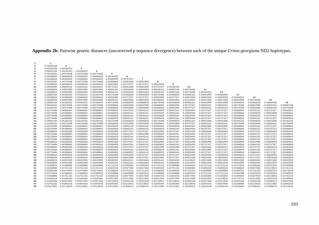
193
Appendix 2b: Pairwise genetic distances (uncorrected p sequence divergence) between each of the unique Crinia georgiana ND2 haplotypes.
1 12 0.00092166 23 0.00092166 0.00184332 34 0.00092166 0.00184332 0.00184332 45 0.00184332 0.00276498 0.00276498 0.00276498 56 0.00368664 0.00460829 0.00460829 0.00460829 0.00184332 67 0.00368664 0.00460829 0.00460829 0.00460829 0.00552995 0.00737327 78 0.00184332 0.00276498 0.00276498 0.00276498 0.00368664 0.00552995 0.00552995 89 0.00368664 0.00460829 0.00460829 0.00460829 0.00552995 0.00737327 0.00737327 0.00552995 9
10 0.00552995 0.00645161 0.00645161 0.00645161 0.00737327 0.00921659 0.00921659 0.00737327 0.00184332 1011 0.00460829 0.00552995 0.00552995 0.00552995 0.00645161 0.00829493 0.00829493 0.00645161 0.00092166 0.00276498 1112 0.00460829 0.00552995 0.00552995 0.00552995 0.00645161 0.00829493 0.00829493 0.00645161 0.00092166 0.00276498 0.00184332 1213 0.00092166 0.00184332 0.00184332 0.00184332 0.00276498 0.00460829 0.00460829 0.00276498 0.00460829 0.00645161 0.00552995 0.00552995 1314 0.00368664 0.00460829 0.00460829 0.00460829 0.00552995 0.00737327 0.00737327 0.00552995 0.00737327 0.00921659 0.00829493 0.00829493 0.00460829 1415 0.00460829 0.00552995 0.00552995 0.00552995 0.00645161 0.00829493 0.00829493 0.00460829 0.00829493 0.01013825 0.00921659 0.00921659 0.00552995 0.00276498 1516 0.00092166 0.00184332 0.00184332 0.00184332 0.00276498 0.00460829 0.00460829 0.00276498 0.00460829 0.00645161 0.00552995 0.00552995 0.00184332 0.00460829 0.00552995 1617 0.00184332 0.00276498 0.00276498 0.00276498 0.00368664 0.00552995 0.00552995 0.00368664 0.00552995 0.00737327 0.00645161 0.00645161 0.00276498 0.00552995 0.00645161 0.0009216618 0.00184332 0.00276498 0.00276498 0.00276498 0.00368664 0.00552995 0.00552995 0.00368664 0.00552995 0.00737327 0.00645161 0.00645161 0.00276498 0.00552995 0.00645161 0.0027649819 0.00276498 0.00368664 0.00368664 0.00368664 0.00460829 0.00645161 0.00645161 0.00460829 0.00645161 0.00829493 0.00737327 0.00737327 0.00368664 0.00645161 0.00737327 0.0036866420 0.00276498 0.00368664 0.00368664 0.00368664 0.00460829 0.00645161 0.00645161 0.00460829 0.00645161 0.00829493 0.00737327 0.00737327 0.00368664 0.00460829 0.00552995 0.0036866421 0.00276498 0.00368664 0.00368664 0.00368664 0.00460829 0.00645161 0.00645161 0.00460829 0.00645161 0.00829493 0.00737327 0.00737327 0.00368664 0.00645161 0.00737327 0.0036866422 0.00276498 0.00368664 0.00368664 0.00368664 0.00460829 0.00645161 0.00645161 0.00460829 0.00645161 0.00829493 0.00737327 0.00737327 0.00368664 0.00645161 0.00737327 0.0036866423 0.00092166 0.00184332 0.00184332 0.00184332 0.00276498 0.00460829 0.00460829 0.00276498 0.00460829 0.00645161 0.00552995 0.00552995 0.00184332 0.00460829 0.00552995 0.0018433224 0.00184332 0.00276498 0.00276498 0.00276498 0.00368664 0.00552995 0.00552995 0.00368664 0.00552995 0.00737327 0.00645161 0.00645161 0.00276498 0.00552995 0.00645161 0.0027649825 0.00276498 0.00368664 0.00368664 0.00368664 0.00460829 0.00645161 0.00645161 0.00460829 0.00460829 0.00645161 0.00552995 0.00552995 0.00368664 0.00645161 0.00737327 0.0036866426 0.00276498 0.00368664 0.00368664 0.00368664 0.00460829 0.00645161 0.00645161 0.00460829 0.00645161 0.00829493 0.00737327 0.00737327 0.00368664 0.00645161 0.00737327 0.0036866427 0.00368664 0.00460829 0.00460829 0.00460829 0.00552995 0.00737327 0.00737327 0.00552995 0.00737327 0.00921659 0.00829493 0.00829493 0.00460829 0.00737327 0.00829493 0.0046082928 0.00276498 0.00368664 0.00368664 0.00368664 0.00460829 0.00645161 0.00552995 0.00460829 0.00645161 0.00829493 0.00737327 0.00737327 0.00368664 0.00645161 0.00737327 0.0036866429 0.00276498 0.00368664 0.00368664 0.00368664 0.00460829 0.00645161 0.00645161 0.00368664 0.00645161 0.00829493 0.00737327 0.00737327 0.00368664 0.00645161 0.00737327 0.0036866430 0.00276498 0.00368664 0.00368664 0.00368664 0.00460829 0.00645161 0.00645161 0.00460829 0.00645161 0.00829493 0.00737327 0.00737327 0.00368664 0.00645161 0.00737327 0.0036866431 0.00368664 0.00460829 0.00460829 0.00460829 0.00552995 0.00737327 0.00737327 0.00552995 0.00737327 0.00921659 0.00829493 0.00829493 0.00460829 0.00552995 0.00829493 0.0046082932 0.00276498 0.00368664 0.00368664 0.00368664 0.00460829 0.00645161 0.00645161 0.00460829 0.00645161 0.00829493 0.00737327 0.00737327 0.00368664 0.00645161 0.00737327 0.0036866433 0.00368664 0.00460829 0.00460829 0.00460829 0.00552995 0.00737327 0.00737327 0.00552995 0.00552995 0.00737327 0.00645161 0.00645161 0.00460829 0.00737327 0.00829493 0.0046082934 0.00276498 0.00368664 0.00368664 0.00368664 0.00460829 0.00645161 0.00645161 0.00460829 0.00645161 0.00829493 0.00552995 0.00737327 0.00368664 0.00645161 0.00737327 0.0036866435 0.00276498 0.00368664 0.00368664 0.00368664 0.00460829 0.00460829 0.00645161 0.00460829 0.00645161 0.00829493 0.00737327 0.00737327 0.00368664 0.00645161 0.00737327 0.0036866436 0.00368664 0.00460829 0.00460829 0.00460829 0.00552995 0.00552995 0.00737327 0.00552995 0.00737327 0.00921659 0.00829493 0.00829493 0.00460829 0.00737327 0.00829493 0.0046082937 0.00368664 0.00460829 0.00460829 0.00460829 0.00552995 0.00552995 0.00737327 0.00552995 0.00737327 0.00921659 0.00829493 0.00829493 0.00460829 0.00737327 0.00829493 0.0046082938 0.00460829 0.00552995 0.00552995 0.00552995 0.00645161 0.00645161 0.00829493 0.00645161 0.00829493 0.01013825 0.00921659 0.00921659 0.00552995 0.00829493 0.00921659 0.0055299539 0.00460829 0.00552995 0.00552995 0.00552995 0.00645161 0.00645161 0.00829493 0.00645161 0.00829493 0.01013825 0.00921659 0.00921659 0.00552995 0.00829493 0.00921659 0.0055299540 0.01566820 0.01658986 0.01658986 0.01658986 0.01751152 0.01935484 0.01935484 0.01751152 0.01658986 0.01843318 0.01751152 0.01751152 0.01474654 0.01935484 0.02027650 0.0165898641 0.01658986 0.01751152 0.01751152 0.01751152 0.01843318 0.02027650 0.02027650 0.01843318 0.01751152 0.01935484 0.01843318 0.01843318 0.01566820 0.02027650 0.02119816 0.0175115242 0.01382488 0.01474654 0.01474654 0.01474654 0.01566820 0.01751152 0.01751152 0.01566820 0.01566820 0.01751152 0.01658986 0.01658986 0.01290323 0.01751152 0.01843318 0.0147465443 0.01474654 0.01566820 0.01566820 0.01566820 0.01658986 0.01658986 0.01843318 0.01658986 0.01658986 0.01843318 0.01751152 0.01751152 0.01382488 0.01843318 0.01935484 0.0156682044 0.01658986 0.01751152 0.01751152 0.01751152 0.01843318 0.02027650 0.02027650 0.01843318 0.01843318 0.02027650 0.01935484 0.01935484 0.01566820 0.02027650 0.02119816 0.0175115245 0.01843318 0.01935484 0.01935484 0.01935484 0.02027650 0.02211982 0.02211982 0.02027650 0.02027650 0.02211982 0.01935484 0.02119816 0.01751152 0.02211982 0.02304148 0.0193548446 0.01935484 0.02027650 0.02027650 0.02027650 0.02119816 0.02304148 0.02304148 0.02119816 0.02119816 0.02304148 0.02027650 0.02211982 0.01843318 0.02304148 0.02396313 0.0202765047 0.01751152 0.01843318 0.01843318 0.01843318 0.01935484 0.02119816 0.02119816 0.01935484 0.01935484 0.02119816 0.01843318 0.02027650 0.01658986 0.02119816 0.02211982 0.0184331848 0.02027650 0.02119816 0.02119816 0.02119816 0.02211982 0.02396313 0.02396313 0.02211982 0.02211982 0.02396313 0.02304148 0.02304148 0.01935484 0.02396313 0.02488479 0.02119816

194

195
Appendix 2b Cont.: Pairwise genetic distances (uncorrected p sequence divergence) between each of the unique Crinia georgiana ND2haplotypes continued.
33 3334 0.00368664 3435 0.00460829 0.00368664 3536 0.00552995 0.00460829 0.00092166 3637 0.00552995 0.00460829 0.00092166 0.00184332 3738 0.00645161 0.00552995 0.00184332 0.00276498 0.00276498 3839 0.00645161 0.00552995 0.00184332 0.00276498 0.00276498 0.00368664 3940 0.01382488 0.01566820 0.01658986 0.01751152 0.01751152 0.01843318 0.01843318 4041 0.01474654 0.01658986 0.01751152 0.01843318 0.01843318 0.01935484 0.01935484 0.00092166 4142 0.01382488 0.01474654 0.01474654 0.01566820 0.01566820 0.01658986 0.01658986 0.00184332 0.00276498 4243 0.01474654 0.01566820 0.01566820 0.01658986 0.01658986 0.01751152 0.01751152 0.00276498 0.00368664 0.00092166 4344 0.01658986 0.01751152 0.01566820 0.01658986 0.01658986 0.01751152 0.01751152 0.00460829 0.00552995 0.00276498 0.00368664 4445 0.01843318 0.01751152 0.01751152 0.01843318 0.01843318 0.01935484 0.01935484 0.00645161 0.00737327 0.00460829 0.00552995 0.00184332 4546 0.01935484 0.01843318 0.01843318 0.01935484 0.01935484 0.02027650 0.02027650 0.00737327 0.00829493 0.00552995 0.00645161 0.00276498 0.00092166 4647 0.01751152 0.01658986 0.01658986 0.01751152 0.01751152 0.01843318 0.01843318 0.00737327 0.00829493 0.00552995 0.00645161 0.00276498 0.00092166 0.00184332 4748 0.02027650 0.02119816 0.01935484 0.02027650 0.02027650 0.02119816 0.02119816 0.00829493 0.00921659 0.00645161 0.00737327 0.00552995 0.00737327 0.00829493 0.00829493 48
17 1718 0.00368664 1819 0.00460829 0.00092166 1920 0.00460829 0.00092166 0.00184332 2021 0.00460829 0.00276498 0.00368664 0.00368664 2122 0.00460829 0.00460829 0.00552995 0.00552995 0.00552995 2223 0.00276498 0.00276498 0.00368664 0.00368664 0.00368664 0.00368664 2324 0.00368664 0.00368664 0.00460829 0.00460829 0.00460829 0.00460829 0.00092166 2425 0.00460829 0.00460829 0.00552995 0.00552995 0.00552995 0.00552995 0.00184332 0.00276498 2526 0.00460829 0.00460829 0.00552995 0.00552995 0.00552995 0.00552995 0.00184332 0.00276498 0.00184332 2627 0.00552995 0.00552995 0.00645161 0.00645161 0.00645161 0.00645161 0.00276498 0.00368664 0.00276498 0.00092166 2728 0.00460829 0.00460829 0.00552995 0.00552995 0.00552995 0.00552995 0.00184332 0.00276498 0.00184332 0.00184332 0.00276498 2829 0.00460829 0.00460829 0.00552995 0.00552995 0.00552995 0.00552995 0.00184332 0.00276498 0.00184332 0.00184332 0.00276498 0.00184332 2930 0.00460829 0.00460829 0.00552995 0.00552995 0.00552995 0.00552995 0.00184332 0.00276498 0.00184332 0.00184332 0.00276498 0.00184332 0.00184332 3031 0.00552995 0.00552995 0.00645161 0.00645161 0.00645161 0.00645161 0.00276498 0.00368664 0.00276498 0.00276498 0.00368664 0.00276498 0.00276498 0.00092166 3132 0.00460829 0.00460829 0.00552995 0.00552995 0.00552995 0.00552995 0.00184332 0.00276498 0.00184332 0.00184332 0.00276498 0.00184332 0.00184332 0.00184332 0.00276498 3233 0.00552995 0.00552995 0.00645161 0.00645161 0.00645161 0.00645161 0.00276498 0.00368664 0.00276498 0.00276498 0.00368664 0.00276498 0.00276498 0.00276498 0.00368664 0.0027649834 0.00460829 0.00460829 0.00552995 0.00552995 0.00552995 0.00552995 0.00276498 0.00368664 0.00276498 0.00276498 0.00368664 0.00276498 0.00276498 0.00276498 0.00368664 0.0027649835 0.00460829 0.00460829 0.00552995 0.00552995 0.00552995 0.00552995 0.00368664 0.00460829 0.00368664 0.00368664 0.00460829 0.00368664 0.00368664 0.00368664 0.00460829 0.0036866436 0.00552995 0.00552995 0.00645161 0.00645161 0.00645161 0.00645161 0.00460829 0.00552995 0.00460829 0.00460829 0.00552995 0.00460829 0.00460829 0.00460829 0.00552995 0.0046082937 0.00552995 0.00552995 0.00645161 0.00645161 0.00645161 0.00645161 0.00460829 0.00552995 0.00460829 0.00460829 0.00552995 0.00460829 0.00460829 0.00460829 0.00552995 0.0046082938 0.00645161 0.00460829 0.00552995 0.00552995 0.00552995 0.00737327 0.00552995 0.00645161 0.00552995 0.00552995 0.00645161 0.00552995 0.00552995 0.00552995 0.00645161 0.0055299539 0.00645161 0.00645161 0.00737327 0.00737327 0.00737327 0.00737327 0.00552995 0.00645161 0.00552995 0.00552995 0.00645161 0.00552995 0.00552995 0.00552995 0.00645161 0.0055299540 0.01751152 0.01751152 0.01843318 0.01843318 0.01843318 0.01843318 0.01474654 0.01474654 0.01474654 0.01290323 0.01382488 0.01474654 0.01474654 0.01474654 0.01566820 0.0147465441 0.01843318 0.01843318 0.01935484 0.01935484 0.01935484 0.01935484 0.01566820 0.01566820 0.01566820 0.01382488 0.01474654 0.01566820 0.01566820 0.01566820 0.01658986 0.0156682042 0.01566820 0.01566820 0.01658986 0.01658986 0.01658986 0.01658986 0.01474654 0.01474654 0.01474654 0.01290323 0.01382488 0.01474654 0.01474654 0.01474654 0.01566820 0.0147465443 0.01658986 0.01658986 0.01751152 0.01751152 0.01751152 0.01751152 0.01566820 0.01566820 0.01566820 0.01382488 0.01474654 0.01566820 0.01566820 0.01566820 0.01658986 0.0156682044 0.01843318 0.01843318 0.01935484 0.01935484 0.01935484 0.01935484 0.01751152 0.01751152 0.01751152 0.01566820 0.01658986 0.01751152 0.01751152 0.01751152 0.01843318 0.0175115245 0.02027650 0.02027650 0.02119816 0.02119816 0.02119816 0.02119816 0.01935484 0.01935484 0.01935484 0.01751152 0.01843318 0.01935484 0.01935484 0.01935484 0.02027650 0.0193548446 0.02119816 0.02119816 0.02211982 0.02211982 0.02211982 0.02211982 0.02027650 0.02027650 0.02027650 0.01843318 0.01935484 0.02027650 0.02027650 0.02027650 0.02119816 0.0202765047 0.01935484 0.01935484 0.02027650 0.02027650 0.02027650 0.02027650 0.01843318 0.01843318 0.01843318 0.01658986 0.01751152 0.01843318 0.01843318 0.01843318 0.01935484 0.0184331848 0.02211982 0.02211982 0.02304148 0.02304148 0.02304148 0.02304148 0.02119816 0.02119816 0.02119816 0.01935484 0.02027650 0.02119816 0.02119816 0.02119816 0.02211982 0.02119816
33 3334 0.00368664 3435 0.00460829 0.00368664 3536 0.00552995 0.00460829 0.00092166 3637 0.00552995 0.00460829 0.00092166 0.00184332 3738 0.00645161 0.00552995 0.00184332 0.00276498 0.00276498 3839 0.00645161 0.00552995 0.00184332 0.00276498 0.00276498 0.00368664 3940 0.01382488 0.01566820 0.01658986 0.01751152 0.01751152 0.01843318 0.01843318 4041 0.01474654 0.01658986 0.01751152 0.01843318 0.01843318 0.01935484 0.01935484 0.00092166 4142 0.01382488 0.01474654 0.01474654 0.01566820 0.01566820 0.01658986 0.01658986 0.00184332 0.00276498 4243 0.01474654 0.01566820 0.01566820 0.01658986 0.01658986 0.01751152 0.01751152 0.00276498 0.00368664 0.00092166 4344 0.01658986 0.01751152 0.01566820 0.01658986 0.01658986 0.01751152 0.01751152 0.00460829 0.00552995 0.00276498 0.00368664 4445 0.01843318 0.01751152 0.01751152 0.01843318 0.01843318 0.01935484 0.01935484 0.00645161 0.00737327 0.00460829 0.00552995 0.00184332 4546 0.01935484 0.01843318 0.01843318 0.01935484 0.01935484 0.02027650 0.02027650 0.00737327 0.00829493 0.00552995 0.00645161 0.00276498 0.00092166 4647 0.01751152 0.01658986 0.01658986 0.01751152 0.01751152 0.01843318 0.01843318 0.00737327 0.00829493 0.00552995 0.00645161 0.00276498 0.00092166 0.00184332 4748 0.02027650 0.02119816 0.01935484 0.02027650 0.02027650 0.02119816 0.02119816 0.00829493 0.00921659 0.00645161 0.00737327 0.00552995 0.00737327 0.00829493 0.00829493 48

196

197
Appendix 2c: Pairwise genetic distances (uncorrected p sequence divergence) between each of the unique Metacrinia nichollsi ND2 haplotypes.
1 12 0.00088889 23 0.00177778 0.00088889 34 0.00266667 0.00177778 0.00088889 45 0.00266667 0.00177778 0.00088889 0.00177778 56 0.00266667 0.00355556 0.00266667 0.00355556 0.00177778 67 0.00355556 0.00266667 0.00177778 0.00266667 0.00266667 0.00444444 78 0.00355556 0.00266667 0.00177778 0.00266667 0.00266667 0.00444444 0.00355556 89 0.00355556 0.00266667 0.00177778 0.00266667 0.00266667 0.00444444 0.00355556 0.00177778 9
10 0.00266667 0.00177778 0.00088889 0.00177778 0.00177778 0.00355556 0.00266667 0.00266667 0.00266667 1011 0.00444444 0.00355556 0.00266667 0.00355556 0.00355556 0.00533333 0.00444444 0.00444444 0.00444444 0.00177778 1112 0.00622222 0.00533333 0.00444444 0.00533333 0.00533333 0.00711111 0.00622222 0.00622222 0.00622222 0.00355556 0.00533333 1213 0.00533333 0.00622222 0.00533333 0.00622222 0.00622222 0.00622222 0.00711111 0.00711111 0.00711111 0.00444444 0.00622222 0.00266667 1314 0.00622222 0.00533333 0.00444444 0.00533333 0.00533333 0.00711111 0.00622222 0.00622222 0.00622222 0.00355556 0.00533333 0.00177778 0.0026666715 0.00711111 0.00622222 0.00533333 0.00622222 0.00622222 0.00800000 0.00711111 0.00711111 0.00711111 0.00444444 0.00622222 0.00266667 0.0035555616 0.04622222 0.04533333 0.04444445 0.04533333 0.04355555 0.04533333 0.04622222 0.04444445 0.04622222 0.04533333 0.04711111 0.04533333 0.0462222217 0.03111111 0.03200000 0.03111111 0.03200000 0.03200000 0.03200000 0.03111111 0.03288889 0.03288889 0.03022222 0.03200000 0.03200000 0.0311111118 0.03200000 0.03288889 0.03200000 0.03288889 0.03288889 0.03288889 0.03200000 0.03377778 0.03377778 0.03111111 0.03111111 0.03288889 0.0320000019 0.03111111 0.03200000 0.03111111 0.03200000 0.03200000 0.03200000 0.03111111 0.03288889 0.03288889 0.03200000 0.03200000 0.03377778 0.0328888920 0.03111111 0.03200000 0.03111111 0.03200000 0.03200000 0.03200000 0.03111111 0.03288889 0.03288889 0.03200000 0.03200000 0.03377778 0.0328888921 0.03022222 0.03111111 0.03022222 0.03111111 0.03111111 0.03111111 0.03022222 0.03200000 0.03200000 0.03111111 0.03288889 0.03288889 0.0320000022 0.03200000 0.03288889 0.03200000 0.03288889 0.03288889 0.03288889 0.03200000 0.03377778 0.03377778 0.03288889 0.03466666 0.03466666 0.0337777823 0.03022222 0.03111111 0.03022222 0.03111111 0.03111111 0.03111111 0.03022222 0.03200000 0.03200000 0.03111111 0.03111111 0.03288889 0.0320000024 0.03022222 0.03111111 0.03022222 0.03111111 0.02933333 0.02933333 0.03022222 0.03200000 0.03200000 0.03111111 0.03111111 0.03288889 0.0320000025 0.02755556 0.02844444 0.02755556 0.02844444 0.02844444 0.02844444 0.02755556 0.02933333 0.02933333 0.02844444 0.03022222 0.03022222 0.0293333326 0.02844444 0.02933333 0.02844444 0.02933333 0.02933333 0.02933333 0.02844444 0.03022222 0.03022222 0.02933333 0.03111111 0.03111111 0.03022222
1415 0.00088889 1516 0.04533333 0.04622222 1617 0.03200000 0.03288889 0.05155556 1718 0.03288889 0.03377778 0.05244444 0.00088889 1819 0.03377778 0.03466666 0.05155556 0.00800000 0.00711111 1920 0.03377778 0.03466666 0.05066667 0.00888889 0.00800000 0.00088889 2021 0.03288889 0.03377778 0.05244444 0.00888889 0.00977778 0.00266667 0.00355556 2122 0.03466666 0.03555556 0.05422222 0.01066667 0.01155556 0.00444444 0.00533333 0.00177778 2223 0.03288889 0.03377778 0.04888889 0.00977778 0.00888889 0.00622222 0.00711111 0.00888889 0.01066667 2324 0.03288889 0.03377778 0.04711111 0.01244444 0.01155556 0.00888889 0.00977778 0.01155556 0.01333333 0.00444444 2425 0.03022222 0.03111111 0.04622222 0.00977778 0.01066667 0.00800000 0.00888889 0.00888889 0.01066667 0.00355556 0.00266667 2526 0.03111111 0.03200000 0.04711111 0.00977778 0.01066667 0.00800000 0.00888889 0.00888889 0.01066667 0.00355556 0.00444444 0.00177778

198

199
Appendix 2d: Pairwise genetic distances (uncorrected p sequence divergence) between each of the unique Geocrinia leai ND2 haplotypes.
1 12 0.00178571 23 0.00178571 0.00178571 34 0.00267857 0.00267857 0.00089286 45 0.00357143 0.00357143 0.00178571 0.00267857 56 0.00267857 0.00267857 0.00089286 0.00178571 0.00267857 67 0.00357143 0.00357143 0.00178571 0.00267857 0.00357143 0.00089286 78 0.00357143 0.00357143 0.00178571 0.00267857 0.00357143 0.00267857 0.00357143 89 0.00982143 0.00982143 0.00803571 0.00892857 0.00982143 0.00892857 0.00982143 0.00982143 9
10 0.01071429 0.01071429 0.00892857 0.00982143 0.01071429 0.00982143 0.01071429 0.01071429 0.00089286 1011 0.01250000 0.01250000 0.01071429 0.01160714 0.01250000 0.01160714 0.01250000 0.01250000 0.00267857 0.00357143 1112 0.00535714 0.00535714 0.00357143 0.00446429 0.00535714 0.00446429 0.00535714 0.00535714 0.00803571 0.00892857 0.01071429 1213 0.00625000 0.00625000 0.00446429 0.00535714 0.00625000 0.00535714 0.00625000 0.00625000 0.00892857 0.00982143 0.01160714 0.00267857 1314 0.00803571 0.00625000 0.00625000 0.00714286 0.00803571 0.00714286 0.00803571 0.00625000 0.01071429 0.01160714 0.01339286 0.00446429 0.00357143 1415 0.01250000 0.01250000 0.01071429 0.00982143 0.01250000 0.01160714 0.01250000 0.01071429 0.01160714 0.01250000 0.01428571 0.01071429 0.00982143 0.00982143 1516 0.01160714 0.01160714 0.00982143 0.01071429 0.01160714 0.01071429 0.01160714 0.01160714 0.01071429 0.01160714 0.01339286 0.00803571 0.01071429 0.01250000 0.00982143 1617 0.01250000 0.01250000 0.01071429 0.01160714 0.01250000 0.01160714 0.01250000 0.01250000 0.01160714 0.01250000 0.01428571 0.00892857 0.01160714 0.01339286 0.01071429 0.0008928618 0.01250000 0.01250000 0.01071429 0.01160714 0.01250000 0.01160714 0.01250000 0.01250000 0.01339286 0.01428571 0.01607143 0.00892857 0.01160714 0.01339286 0.01250000 0.0026785719 0.01339286 0.01339286 0.01160714 0.01250000 0.01339286 0.01250000 0.01339286 0.01160714 0.01339286 0.01428571 0.01607143 0.01071429 0.01339286 0.01339286 0.01071429 0.0062500020 0.02142857 0.02142857 0.01964286 0.02053571 0.01964286 0.02053571 0.02142857 0.01964286 0.02053571 0.02142857 0.02321429 0.01964286 0.02053571 0.02053571 0.01607143 0.0133928621 0.02232143 0.02232143 0.02053571 0.02142857 0.02232143 0.02142857 0.02232143 0.02053571 0.02142857 0.02232143 0.02410714 0.02053571 0.02142857 0.02142857 0.01875000 0.0160714322 0.02232143 0.02232143 0.02053571 0.02142857 0.02232143 0.02142857 0.02232143 0.02053571 0.02142857 0.02232143 0.02410714 0.02053571 0.02142857 0.02142857 0.01875000 0.0160714323 0.02321429 0.02321429 0.02142857 0.02232143 0.02321429 0.02232143 0.02321429 0.02142857 0.02410714 0.02500000 0.02678571 0.02321429 0.02410714 0.02410714 0.02142857 0.0187500024 0.00982143 0.00982143 0.00803571 0.00892857 0.00982143 0.00892857 0.00982143 0.00982143 0.00982143 0.01071429 0.01250000 0.00803571 0.00714286 0.00892857 0.01071429 0.0116071425 0.01071429 0.01071429 0.00892857 0.00982143 0.01071429 0.00982143 0.01071429 0.01071429 0.01071429 0.01160714 0.01339286 0.00892857 0.00982143 0.01160714 0.01339286 0.0125000026 0.01339286 0.01339286 0.01160714 0.01250000 0.01339286 0.01250000 0.01339286 0.01160714 0.01339286 0.01428571 0.01607143 0.01160714 0.01071429 0.01250000 0.01428571 0.0151785727 0.02410714 0.02410714 0.02232143 0.02321429 0.02410714 0.02321429 0.02410714 0.02232143 0.02500000 0.02589286 0.02767857 0.02232143 0.02321429 0.02321429 0.02053571 0.0178571428 0.02321429 0.02321429 0.02142857 0.02232143 0.02321429 0.02232143 0.02321429 0.02142857 0.02410714 0.02500000 0.02678571 0.02142857 0.02232143 0.02232143 0.01964286 0.0169642929 0.02410714 0.02410714 0.02232143 0.02321429 0.02410714 0.02321429 0.02410714 0.02232143 0.02500000 0.02589286 0.02767857 0.02232143 0.02321429 0.02321429 0.02053571 0.0178571430 0.02321429 0.02321429 0.02142857 0.02232143 0.02321429 0.02232143 0.02321429 0.02142857 0.02232143 0.02321429 0.02500000 0.02142857 0.02232143 0.02232143 0.01964286 0.0169642931 0.02142857 0.02142857 0.01964286 0.02053571 0.02142857 0.02053571 0.02142857 0.02142857 0.01964286 0.02053571 0.02232143 0.02053571 0.02142857 0.02321429 0.01696429 0.0178571432 0.01964286 0.01964286 0.01785714 0.01875000 0.01964286 0.01875000 0.01964286 0.01964286 0.01785714 0.01875000 0.02053571 0.01875000 0.01964286 0.02142857 0.01517857 0.0160714333 0.02321429 0.02142857 0.02142857 0.02232143 0.02321429 0.02232143 0.02321429 0.02321429 0.02142857 0.02232143 0.02410714 0.02232143 0.02321429 0.02142857 0.01875000 0.0178571434 0.02321429 0.02321429 0.02142857 0.02232143 0.02321429 0.02232143 0.02321429 0.02142857 0.02053571 0.02142857 0.02321429 0.02142857 0.02232143 0.02232143 0.01607143 0.0187500035 0.02589286 0.02589286 0.02410714 0.02500000 0.02589286 0.02500000 0.02589286 0.02410714 0.02321429 0.02410714 0.02589286 0.02410714 0.02321429 0.02321429 0.01696429 0.0214285736 0.0250000 0.02500000 0.02321429 0.02410714 0.02500000 0.02410714 0.02500000 0.02321429 0.02232143 0.02321429 0.02500000 0.02321429 0.02232143 0.02232143 0.01607143 0.0205357137 0.05267857 0.05267857 0.05089286 0.05000000 0.05267857 0.05178571 0.05267857 0.05089286 0.05000000 0.05089286 0.05089286 0.05267857 0.05357143 0.05357143 0.04732143 0.0500000038 0.05178571 0.05178571 0.05000000 0.04910714 0.05178571 0.05089286 0.05178571 0.05000000 0.04910714 0.05000000 0.05000000 0.05178571 0.05267857 0.05267857 0.04642857 0.0491071439 0.05267857 0.05267857 0.05089286 0.05000000 0.05267857 0.05178571 0.05267857 0.05089286 0.04821429 0.04910714 0.04910714 0.05089286 0.05178571 0.05178571 0.04553571 0.0482142940 0.05267857 0.05267857 0.05089286 0.05178571 0.05267857 0.05178571 0.05267857 0.05089286 0.04821429 0.04910714 0.04910714 0.05089286 0.05178571 0.05178571 0.04732143 0.0482142941 0.05446428 0.05446428 0.05267857 0.05178571 0.05446428 0.05357143 0.05446428 0.05267857 0.05000000 0.05089286 0.05089286 0.05267857 0.05357143 0.05357143 0.04732143 0.0500000042 0.05267857 0.05267857 0.05089286 0.05178571 0.05267857 0.05000000 0.05089286 0.05089286 0.05000000 0.05089286 0.05089286 0.05089286 0.05178571 0.05178571 0.04910714 0.0500000043 0.05178571 0.05178571 0.05000000 0.05089286 0.05178571 0.05089286 0.05178571 0.05000000 0.04910714 0.05000000 0.05000000 0.05000000 0.05089286 0.05089286 0.04821429 0.0491071444 0.05089286 0.05089286 0.04910714 0.05000000 0.05089286 0.05000000 0.05089286 0.04910714 0.04821429 0.04910714 0.04910714 0.04910714 0.05000000 0.05000000 0.04732143 0.0482142945 0.05178571 0.05178571 0.05000000 0.05089286 0.05178571 0.05089286 0.05178571 0.05000000 0.04910714 0.05000000 0.05000000 0.05000000 0.05089286 0.05089286 0.04821429 0.0491071446 0.06071429 0.06071429 0.05892857 0.05982143 0.06071429 0.05982143 0.06071429 0.05892857 0.05625000 0.05714286 0.05714286 0.06071429 0.05982143 0.05982143 0.05535714 0.0580357147 0.06071429 0.06071429 0.05892857 0.05982143 0.06071429 0.05982143 0.06071429 0.05892857 0.05625000 0.05714286 0.05714286 0.06071429 0.05982143 0.05982143 0.05535714 0.0580357148 0.06250000 0.06250000 0.06071429 0.06160714 0.06250000 0.06160714 0.06250000 0.06071429 0.05803571 0.05892857 0.05892857 0.06250000 0.06160714 0.06160714 0.05714286 0.05982143

200

201
Appendix 2d Cont.: Pairwise genetic distances (uncorrected p sequence divergence) between each of the unique Geocrinia leai ND2 haplotypescontinued.
17 1718 0.00178571 1819 0.00535714 0.00714286 1920 0.01250000 0.01250000 0.01428571 2021 0.01517857 0.01517857 0.01696429 0.00982143 2122 0.01517857 0.01517857 0.01696429 0.00982143 0.00178571 2223 0.01785714 0.01785714 0.01875000 0.01250000 0.00446429 0.00267857 2324 0.01250000 0.01339286 0.01428571 0.01964286 0.02053571 0.02053571 0.02321429 2425 0.01339286 0.01428571 0.01517857 0.02053571 0.02142857 0.02142857 0.02410714 0.00446429 2526 0.01607143 0.01696429 0.01607143 0.02142857 0.02232143 0.02232143 0.02500000 0.00714286 0.00446429 2627 0.01696429 0.01517857 0.01785714 0.01517857 0.01785714 0.01785714 0.02053571 0.02321429 0.02232143 0.02321429 2728 0.01607143 0.01428571 0.01785714 0.01428571 0.01696429 0.01696429 0.01964286 0.02232143 0.02142857 0.02232143 0.00267857 2829 0.01696429 0.01517857 0.01875000 0.01339286 0.01785714 0.01785714 0.02053571 0.02321429 0.02232143 0.02321429 0.00357143 0.00267857 2930 0.01607143 0.01428571 0.01785714 0.01428571 0.01696429 0.01696429 0.01964286 0.02232143 0.02142857 0.02232143 0.00267857 0.00178571 0.00267857 3031 0.01696429 0.01696429 0.01696429 0.01696429 0.01785714 0.01785714 0.01964286 0.02053571 0.02142857 0.02410714 0.01964286 0.01875000 0.01964286 0.01696429 3132 0.01517857 0.01517857 0.01517857 0.01517857 0.01785714 0.01785714 0.01964286 0.01875000 0.01964286 0.02232143 0.01785714 0.01696429 0.01785714 0.01517857 0.00178571 3233 0.01696429 0.01696429 0.01875000 0.01696429 0.01964286 0.01964286 0.02142857 0.02232143 0.02321429 0.02589286 0.01964286 0.01875000 0.01964286 0.01696429 0.00535714 0.0035714334 0.01785714 0.01785714 0.01785714 0.01607143 0.01875000 0.01875000 0.02142857 0.02142857 0.02232143 0.02321429 0.01875000 0.01785714 0.01875000 0.01607143 0.00625000 0.0044642935 0.02053571 0.02053571 0.01875000 0.01696429 0.01964286 0.01964286 0.02232143 0.02232143 0.02500000 0.02589286 0.02142857 0.02053571 0.02142857 0.01875000 0.00892857 0.0071428636 0.02142857 0.02142857 0.02142857 0.01785714 0.02053571 0.02053571 0.02321429 0.02142857 0.02410714 0.02500000 0.02232143 0.02142857 0.02232143 0.01964286 0.00982143 0.0080357137 0.04910714 0.04910714 0.04642857 0.04821429 0.05000000 0.05000000 0.05089286 0.05089286 0.05000000 0.05089286 0.05000000 0.05000000 0.05000000 0.04821429 0.04732143 0.0455357138 0.04821429 0.04821429 0.04553571 0.04732143 0.04910714 0.04910714 0.05000000 0.05000000 0.04910714 0.05000000 0.04910714 0.04910714 0.04910714 0.04732143 0.04642857 0.0446428639 0.04732143 0.04732143 0.04553571 0.04732143 0.04821429 0.04821429 0.05089286 0.04910714 0.04821429 0.04910714 0.04821429 0.04821429 0.04910714 0.04642857 0.04642857 0.0446428640 0.04732143 0.04732143 0.04553571 0.04732143 0.04821429 0.04821429 0.05089286 0.04910714 0.04821429 0.04910714 0.04821429 0.04821429 0.04910714 0.04642857 0.04642857 0.0446428641 0.04910714 0.04910714 0.04732143 0.04910714 0.05000000 0.05000000 0.05267857 0.05089286 0.05000000 0.05089286 0.05000000 0.05000000 0.05089286 0.04821429 0.04821429 0.0464285742 0.04910714 0.04910714 0.04732143 0.05267857 0.05178571 0.05178571 0.05446428 0.05446428 0.05357143 0.05446428 0.05178571 0.05178571 0.05267857 0.05000000 0.04821429 0.0464285743 0.04821429 0.04821429 0.04642857 0.05178571 0.05089286 0.05089286 0.05357143 0.05357143 0.05267857 0.05357143 0.05089286 0.05089286 0.05178571 0.04910714 0.04732143 0.0455357144 0.04732143 0.04732143 0.04553571 0.05089286 0.05178571 0.05178571 0.05446428 0.05267857 0.05178571 0.05267857 0.05000000 0.05000000 0.05089286 0.04821429 0.04642857 0.0446428645 0.04821429 0.04821429 0.04642857 0.05178571 0.05267857 0.05267857 0.05535714 0.05357143 0.05267857 0.05357143 0.05089286 0.05089286 0.05178571 0.04910714 0.04732143 0.0455357146 0.05714286 0.05714286 0.05625000 0.05535714 0.05803571 0.05803571 0.05892857 0.05714286 0.05803571 0.05714286 0.05714286 0.05625000 0.05535714 0.05446428 0.05535714 0.0535714347 0.05714286 0.05714286 0.05625000 0.05535714 0.05625000 0.05803571 0.05892857 0.05714286 0.05803571 0.05714286 0.05714286 0.05625000 0.05535714 0.05446428 0.05535714 0.0535714348 0.05892857 0.05892857 0.05803571 0.05714286 0.05803571 0.05982143 0.06071429 0.05892857 0.05982143 0.05892857 0.05892857 0.05803571 0.05714286 0.05625000 0.05714286 0.05535714
33 3334 0.00803571 3435 0.01071429 0.00803571 3536 0.01160714 0.00892857 0.00267857 3637 0.04910714 0.04732143 0.04821429 0.04910714 3738 0.04821429 0.04642857 0.04732143 0.04821429 0.00089286 3839 0.04821429 0.04553571 0.04642857 0.04732143 0.00892857 0.00803571 3940 0.04821429 0.04553571 0.04642857 0.04732143 0.01071429 0.00982143 0.00357143 4041 0.05000000 0.04732143 0.04821429 0.04910714 0.01071429 0.00982143 0.00357143 0.00357143 4142 0.05000000 0.04732143 0.04821429 0.04910714 0.02232143 0.02142857 0.02053571 0.02053571 0.02232143 4243 0.04910714 0.04642857 0.04732143 0.04821429 0.02142857 0.02053571 0.01964286 0.01964286 0.02142857 0.00089286 4344 0.04821429 0.04553571 0.04642857 0.04732143 0.02053571 0.01964286 0.01875000 0.01875000 0.02053571 0.00178571 0.00089286 4445 0.04910714 0.04642857 0.04732143 0.04821429 0.02142857 0.02053571 0.01785714 0.01785714 0.01964286 0.00267857 0.00178571 0.00089286 4546 0.05714286 0.05535714 0.05446428 0.05357143 0.04821429 0.04910714 0.05178571 0.05000000 0.05357143 0.05982143 0.05892857 0.05803571 0.05892857 4647 0.05714286 0.05535714 0.05446428 0.05357143 0.05000000 0.05089286 0.05357143 0.05178571 0.05535714 0.06160714 0.06071429 0.05982143 0.06071429 0.00178571 4748 0.05892857 0.05714286 0.05625000 0.05535714 0.05178571 0.05267857 0.05357143 0.05357143 0.05714286 0.06339286 0.06250000 0.06160714 0.06250000 0.00357143 0.00178571

203
Appendix 3:
Complete GeoDis v2.4 output for the Nested CladePhylogeographic Analysis for each Data Chapter

204

205
Appendix 3a: Complete GeoDis v 2.4 output for the Arenophryne rotunda (Northern Lineage) Nested Clade Phylogeographic Analysis.
No. Dc Dn No. Dc Dn No. Dc Dn No. Dc Dn1 t 0 02 I 0 0 1-1t 0< 20.003 t 0 37.86>4 t 0< 28.38<I-T 0 -9.7
Int/tip not det 1-2 I 32.44 30.525 t 0 11.146 t 0 16.717 t 0 16.71 1-3 t 13.37< 28..068 0 0 1-4 t 0 51.559 0 0 1-5 t 0< 22.34
I-T 26.71> 4.141-N, 2-Y, 3-N, 4-Y, 9-N - AF 2-1 t 27.43< 26.22<
14 0 0 1-6 0 015 0 016 0 0 1-11 0 017 0 0 1-12 0 0 2-4 I 0< 87.92>
I-T -27.43< 61.70>1-Y, 19-Y, 20-Y, 2-N, 11-Y - RE - 12-Y, 13-Y -LDC 3-1 I 35.47 37.59
10 0 0 1-7 I 0 12.8411 0 0 1-8 I 0 12.83 2-2 I 12.83 12.83
12 0 0 1-9 0 013 0 0 1-10 0 0 2-3 t 0 6.42
I-T 12.83 6.42 3-2 t 9.62< 38.37I-T 25.85> -0.78
1-N, 2-Y, 3-N, 4-N: RGF w/ IBD
3-step cladesHaplotypes 1-step clades 2-step clades

206
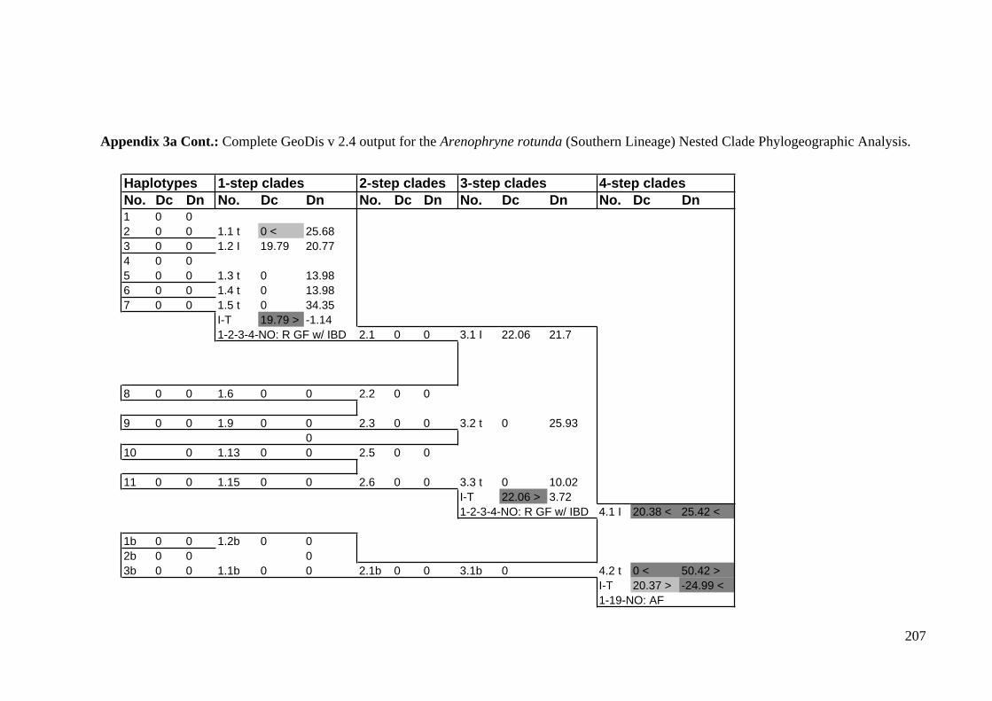
207
Appendix 3a Cont.: Complete GeoDis v 2.4 output for the Arenophryne rotunda (Southern Lineage) Nested Clade Phylogeographic Analysis.Southern Network
Haplotypes 1-step clades 2-step clades 3-step clades 4-step cladesNo. Dc Dn No. Dc Dn No. Dc Dn No. Dc Dn No. Dc Dn1 0 02 0 0 1.1 t 0 < 25.683 0 0 1.2 I 19.79 20.774 0 05 0 0 1.3 t 0 13.986 0 0 1.4 t 0 13.987 0 0 1.5 t 0 34.35
I-T 19.79 > -1.141-2-3-4-NO: R GF w/ IBD 2.1 0 0 3.1 I 22.06 21.7
8 0 0 1.6 0 0 2.2 0 0
9 0 0 1.9 0 0 2.3 0 0 3.2 t 0 25.930
10 0 1.13 0 0 2.5 0 0
11 0 0 1.15 0 0 2.6 0 0 3.3 t 0 10.02I-T 22.06 > 3.721-2-3-4-NO: R GF w/ IBD 4.1 I 20.38 < 25.42 <
1b 0 0 1.2b 0 02b 0 0 03b 0 0 1.1b 0 0 2.1b 0 0 3.1b 0 4.2 t 0 < 50.42 >
I-T 20.37 > -24.99 <1-19-NO: AF

209
Appendix 3b: Complete GeoDis v 2.4 output for the Crinia georgiana Nested CladePhylogeographic Analysis.
Haplotypes 1-step clades 2-step clades 3-step clades 4-step cladesNo. Dc Dn No. Dc Dn No. Dc Dn No. Dc Dn No. Dc Dn
10 0 0 1.1 t 0 14.28
9 I 0 98.7211 t 0 49.5112 t 0 49.51I-T 0 49.21 1.2 I 65.92 64.36
I-T 65.92 50.07 2.1 t 51.84< 124.47
1 I 47.79 45.882 t 63.65> 63.9>3 t 0 43.274 t 0 22.52
13 t 0 22.52I-T 11.42 -3.25 1.10 I 47.78< 73.28<
8 0 0 1.5 t 0 51.75
16 I 0 14.2817 t 0 14.28I-T 0 -0.0012 1.11 t 14.28 31.14
22 0 0 1.4 t 0 263.14
23 I 0 33.9324 t 0 33.98I-T 0 -0.05 1.22 I 33.95 257.65>
I-T 38.66 5.331-N; 2-Y; 3-Y; 5-Y; 15-N-LDC; 21-Y LDM check 21 2.2 I 101.43< 159.1>
7 0 0 0 0 0 2.3 t 0 58.08
6 0 0 1.8 0 0
5 0 0 1.9 0 0 2.4 t 0 98.96
14 0 0 1.14 I 0 35.39
15 0 0 1.13 t 0 47.14I-T 0 -11.74 2.5 t 40.42 78.77
21 0 0 1.15 I 0< 42.10<
18 I 41.27 41.2719 t 0 41.2520 t 0 41.29I-T 41.27 0 1.16 t 41.27 57.48>
I-T -41.27< -15.38<1-Y; 19-Y; 20-Y; 2-N; 11-Y-CRE; 12-N-CRE 2.6 t 49.79< 82.01<
25 t 0 38.9428 I 61.31 62.4529 t 0 60.6932 t 0 64.81I-T 61.31 7.64 1.23 I 58.3 66.57
33 0 0 1.24 t 0 57.18
30 I 0 33.9831 t 0 33.93I-T 0 0.05 1.25 t 33.95 58.85
26 I 121.21 120.0227 t 0 63.01I-T 121.21 57.02 1.26 I 102.92 119.7>
I-T 52.4 28.2> 2.9 I 79.26< 134.48I-T 52.64 57.55>
1-N; 2-N; 11-Y-RE; 12-Y; 13-Y-LDC w/ PF or PF w/ RE; 21-? 3.1 I 128.48 128.05
34 0 0 1.21 0 0 2.7 I 0 122.32
35 I 0 28.836 t 0 63.8137 t 0 85.71I-T 0 -45.96 1.18 I 59.44 62.82
38 0 0 1.19 t 0 73.44
39 0 0 1.20 t 0 38.42I-T 59.44 6.89 2.8 t 60.06 56.06
I-T -60.06 66.25 3.2 t 67.11< 115.83I-T 61.38> 12.22 4.1 I 126.68< 174.13<
40 0 041 0 0 1.33 0 0 2.12 I 0 76.45
42 I 0 105.843 t 0 141.76I-T 0 -35.96 1.34 0 0 2.13 t 121.21 143.96 3.4 I 101.32 240.41>
I-T -121.21 -67.51
44 0 0 1.36 I 0 39.18
45 I 39.19 39.1946 t 0 26.1447 t 0 52.24I-T 39.19 6.53 1.37 t 34.84 39.2
I-T -34.84 -0.02 2.14 I 39.19> 39.77>
48 0 0 1.39 0 0 2.15 t 0 26.12<I-T 39.19> 13.65>
1-Y; 19-N- AF 3.5 t 35.22< 124.47<I-T 66.1 115.95>
1-Y; 19-N-AF 4.2 t 164.52 362.71>I-T -37.83 -188.58<
1-N; 2-N; 11-Y-RE; 12-N-CRE

211
Appendix 3c: Complete GeoDis v 2.4 output for the Metacrinia nichollsi Nested Clade Phylogeographic Analysis.
Haplotypes 1-step clades 2-step clades 3-step cladesNo. Dc Dn No. Dc Dn No. Dc Dn No. Dc Dn
Network B
1 0 02 0 0 1.1 t 0 30.233 I 61.39 61.474 t 0 16.245 I 0 27.51I-T 58.83 43.82 1.2 I 58.61 59.096 0 0 1.5 t 0 9.34<7 0 0 1.4 t 0 59.118 0 09 0 0 1.3 t 0 95.67
I-T 58.61> 15.291-N; 2-Y; 3-N; 4-N-RGF w/ IBD 2.1 t 55.99< 60.14<
10 0 0 1.6 I 0 11.0111 0 0 1.7 t 0 33.01
I-T 0 -21.99 2.2 I 16.51< 85.18
12 0 0 1.8 0 013 0 0 1.9 0 014 0 015 0 0 1.10 0 0 2.3 t 11.02< 107.54>
I-T -34.34 19.621-N; 2-N; 11-Y-RE; 12-Y; 13-Y-LDC w/ F or F w/ RE; 21-?
Network C
17 0 018 0 0 1.11 0 0 2.4 t 0< 56.83>
19 0 020 0 0 1.15 0 0 2.5 I 0< 56.05
21 0 0 1.16 0 022 0 0 1.17 0 0 2.6 t 0< 3.57<
I-T 0 25.861-N; 2-N; 11-Y-RE; 12-N-CRE 3.2 I 38.82< 60.63<
23 0 0 1.19 0 0 2.7 0 0
24 0 0 1.22 0 0
25 0 0 1.20 0 0
26 0 0 1.21 0 0 2.8 0 0 3.3 t 0< 160.37>I-T 38.82 -99.74<
1-Y; 19-Y; 20-Y; 2-N; 11-Y-RE; 12-Y; 13-Y-LDC w/ F or PF w/ RE; 21-?

212

213
Appendix 3d: Complete GeoDis v 2.4 output for the Geocrinia leai (Western Lineage Only) Nested Clade Phylogeographic Analysis.
Haplotypes 1-step clades 2-step clades 3-step clades 4-step clades 5-step clades 6-step cladesNo. Dc Dn No. Dc Dn No. Dc Dn No. Dc Dn No. Dc Dn No. Dc Dn No. Dc Dn1 t 0 02 t 0 0 1.1 t 0 4.803 I 0 04 t 0 0 1.3 I 0 19.365 t 0 0 1.2 t 0 4.86 I 0 07 t 0 1.5 t 23.91 23.718 t 0 0 1.4 t 0 29.5
IT -7.97 4.14 2.1 I 0 0 3.1 I 15.57< 22.04<
9 I 0 010 t 0 0 1.10 I 0 011 t 0 0 1.11 t 0 0 2.4 t 0 0 3.2 t 0< 50.87>
IT 15.57 -28.84<1-Y; 19-Y; 20-N - IGS 4.1 t 30.28< 40.13<
12 t 0 0 1.12 I 0 108.9313 t 0 0 1.13 I 0 108.98 2.5 I 108.95 109.16
24 t 0 0 1.42 I 0 0 2.6 I 0 39.07 3.3 I 85.80 80.91
25 t 0 0 1.44 I 0 0 2.7 I 0 0
26 t 0 0 1.46 t 0 0 2.8 t 0 0 3.4 t 0 23.44IT 85.80 57.47 4.2 I 57.92 99.15>
IT 27.65 -59.02<1 - N; 2 - Y; 3 - Y; 5 - Y; 15 - N - PF &/OR LDC - 21 - 5.1 t 52.26< 71.11<
14 t 0 0 1.15 t 0 0 2.9 I 0 82.81
15 t 0 0 1.19 t 0 0 2.11 t 0 82.74I-T 0 0.07 3.5 I 82.78 96.96
16 I 0 017 I 0 0 1.23 I 0 0 2.13 I 0 14.80
18 t 0 0 1.26 t 0 0 2.14 t 0 29.60IT 0 -14.80 3.6 I 19.73 48.72
19 t 0 0 1.27 I 0 0 2.15 I 0 0 3.7 I 0 47.82 4.3 I 64.65 63.84
20 t 0 0 1.33 t 0 0 2.18 t 0 0 3.8 I 0 0
21 t 0 0 1.37 I 0 0 2.19 I 0 0
22 I 0 0 1.38 I 0 023 t 0 0 1.38 t 0 0 2.20 t 0 0 3.9 t 0 0 4.4 t 0< 46.40
IT 64.65> 17.431-Y; 19-Y; 20-N - IGS 5.2 t 54.53< 99.96>
I-T 2.26 28.01<1 - N; 2 - N; 11 - Y - RE; 12 - Y; 13 - Y - LDC w/ F OR PF w/ RE; 21 - 6.1 I 82.06< 86.05
27 t 0 0 1.47 t 0 028 t 0 030 t 0 0 1.48 I 0 029 t 0 0 1.49 t 0 0 2.21 t 0 0 3.10 t 0 0 4.5 t 0 0 5.3 t 0 0 6.2 t 0< 99.69
31 t 0 0 1.50 t 0 032 I 0 0 1.51 I 0 0 2.22 I 0 11.5
33 t 0 0 1.53 t 0 0 2.23 t 0 11.5
34 t 0 0 1.55 t 0 0 2.24 I 0 45.99I-T 0 8.62 3.11 t 18.4 26.28
35 t 0 0 1.58 I 0 0 3.12 t 0 32.8536 t 0 0 1.59 t 0 0 2.26 t 0 0 I-T 18.4 -6.57 4.6 t 0 0 5.4 t 0 0 6.3 t 28.16< 99.6
I-T 64.14> -13.581 - N; 2 - Y; 3 - N; 4 - Y; 9 - Y - AF

215
Appendix 4:
Supplementary Tests for Nested Clade PhylogeographicAnalysis to assess Secondary Contact
for each Data Chapter

216

217
Appendix 4a: Mean pairwise distances (km) between geographical clade centres found ateach Arenophryne rotunda (Northern Lineage) sampling location at various nesting levels.Sites where geographically divergent clades (i.e. high distance values) are present relativeto the distribution of the lineage represent sites of secondary contact between divergentlineages. For principles and methodology behind this supplementary test for NCPA seeTempleton (2001).
1 Step Clades
0
5
10
15
20
25
30
35
40
DHN DHM DHS SP FE2 PC EL1 WW
Collection Sites
Mean
Pair
wis
e D
ista
nce
b
/w
Cla
des
(km
)
2 Step Clades
0
10
20
30
40
50
60
DHN DHM DHS SP FE2 PC EL1 WW
Sampling Location
Mean
Pair
wis
e D
ista
nce
b
/w
Cla
des
(km
)
3 Step Clades
0
5
10
15
20
25
30
35
40
45
50
DHN DHM DHS SP FE2 PC EL1 WW
Sampling Location
Mean
Pair
wis
e D
ista
nce
b
/w
Cla
des
(km
)

218

219
Appendix 4b: Mean pairwise distances (km) between geographical clade centres found ateach Crinia georgiana sampling location at various nesting levels. Sites wheregeographically divergent clades (i.e. high distance values) are present relative to thedistribution of the species represent sites of secondary contact between divergent lineages.For principles and methodology behind this supplementary test for NCPA see Templeton(2001). Only clade levels with a possible inference of secondary contact are shown.
2 Step Clades
0
50
100
150
200
250
MO SA
SP
MU
R
HW
CO
L
NR
BW BE
DW SG DF
KH
KA
L
BB
CLG MIS
CA
NP
Sampling Location
Mean
Pair
wis
e D
ista
nce
sb
/w
Cla
des
(km
)
3 Step Clades
0
50
100
150
200
250
MO SA
SP
MU
R
HW
CO
L
NR
BW BE
DW SG DF
KH
KA
L
BB
CLG MIS
CA
NP
Sampling Location
Mean
Pair
wis
e D
ista
nce
s b
/w
Cla
des
(km
)
Total Cladogram
0
50
100
150
200
250
300
350
400
450
500
MO SA
SP
MU
R
HW
CO
L
NR
BW BE
DW SG DF
KH
KA
L
BB
CLG MIS
CA
NP
Sampling Locations
Mean
Pair
wis
e D
ista
nce
s b
/w
Cla
des
(km
)

220

221
Appendix 4c: Mean pairwise distances (km) between geographical clade centres found ateach Metacrinia nichollsi (Main Range Lineage) sampling location at various nestinglevels. Sites where geographically divergent clades (i.e. high distance values) are presentrelative to the distribution of the lineage represent sites of secondary contact betweendivergent lineages. For principles and methodology behind this supplementary test forNCPA see Templeton (2001).
1 Step Clades
0
20
40
60
80
100
120
NR
N
NR
M
NR
S
BS
SA
B
BN
DW
N
DW
S
SG
N
SG
S
DFN
DFS
KH
N
KH
S
KA
LS
Sampling Location
Mean
Pair
wis
e D
ista
nce
b
/w
Cla
des
(km
)
2 Step Clades
0
20
40
60
80
100
120
NR
N
NR
M
NR
S
BS
SA
B
BN
DW
N
DW
S
SG
N
SG
S
DFN
DFS
KH
N
KH
S
KA
LS
Samplng Location
Mean
Pair
wis
e D
ista
nce
b
/w
Cla
des
(km
)

222

223
Appendix 4d: Mean pairwise distances (km) between geographical clade centres found ateach Geocrinia leai (Western Lineage) sampling location at various nesting levels. Siteswhere geographically divergent clades (i.e. high distance values) are present relative to thedistribution of the lineage represent sites of secondary contact between divergent lineages.For principles and methodology behind this supplementary test for NCPA see Templeton(2001).
1 Step Clades
0
5
10
15
20
25
30
SA
SE
RP
MU
R
HW
CO
L
NR
BS
BM BN
DW
Sampling Location
Mean
Pair
wis
eD
ista
nce
s b
/w
Cla
des
(km
)
2 Step Clades
0
10
20
30
40
50
60
70
80
90
SA
SE
RP
MU
R
HW
CO
L
NR
BS
BM BN
DW
Sampling Location
Mean
Pair
wis
e D
ista
nce
s b
/w
Cla
des
(km
)
3 Step Clades
0
10
20
30
40
50
60
70
80
90
100
SA
SE
RP
MU
R
HW
CO
L
NR
BS
BM BN
DW
Sampling Location
Mean
Pair
wis
e D
ista
nce
s b
/w
Cla
des
(km
)

224

225
Appendix 4d Cont.: Mean pairwise distances (km) between geographical clade centresfound at each Geocrinia leai (Western Lineage) sampling location at various nesting levels.Sites where geographically divergent clades (i.e. high distance values) are present relativeto the distribution of the lineage represent sites of secondary contact between divergentlineages. For principles and methodology behind this supplementary test for NCPA seeTempleton (2001).
4 Step Clades
0
10
20
30
40
50
60
70
80
90
SA
SE
RP
MU
R
HW
CO
L
NR
BS
BM BN
DW
Sampling Location
Mean
Pair
wis
e D
ista
nce
s b
/w
Cla
des
(km
)
5 Step Clades
0
20
40
60
80
100
120
140
SA
SE
RP
MU
R
HW
CO
L
NR
BS
BM BN
DW
Sampling Location
Mean
Pair
wis
e D
ista
nce
s b
/w
Cla
des
(km
)
Total Cladogram
0
20
40
60
80
100
120
140
SA
SE
RP
MU
R
HW
CO
L
NR
BS
BM BN
DW
Sampling Location
Mean
Pair
wis
e D
ista
nce
s b
/w
Cla
des
(km
)

226

227
The end…