biogeochemistry of iron philip boyd niwa/otago · fe biogeochemistry – 2 solas case studies...
TRANSCRIPT

OUTLINE
Why Iron?
Sources and sinks of iron
The intricacies of Fe chemistry
Fe biogeochemistry – 2 SOLAS case studies
Climate change and Fe biogeochemistry
THE
BIOGEOCHEMISTRY
OF IRON
Philip Boyd
NIWA/Otago
New Zealand
Sept
2011

WHY IRON?
A trace element of
pivotal importance
for phytoplankton
physiology
Images courtesy
B Twining (Bigelow)
Fe:C molar
ratio of 1 x 10⁻⁵

“Give me a tanker of iron, and I’ll give you an Ice Age.”
WHY IRON? Fe:C molar ratio of 1 x 10⁻⁵

Behrenfeld et al. (1996)
High profile but controversial
Courtesy J. Cullen (WHOI 2007)

0.5
1.0
1.5
Fe (
mol/k
g ic
e)
180
200
220
240
260
280
300
[CO
2]
(ppm
v)
20 40 60 80 100 120 140 160
Age (1000 yr)
Iron
CO2
The Vostok ice core provided tantalising evidence
of the impact of changes in Fe supply on atmospheric
CO2 (Martin, 1990)
Today

IRON & CLIMATE
Marine biota play a key role in climate
by regulating atmospheric CO2 levels
One means of regulation is via the
BIOLOGICAL PUMP
The PUMP works most
efficiently when all of
the available nutrients
are utilised

0.5
1.0
1.5
Fe (
mol/k
g ic
e)
180
200
220
240
260
280
300
[CO
2]
(ppm
v)
20 40 60 80 100 120 140 160
Age (1000 yr)
Iron
CO2
Links between iron and climate

ODP (red) & EPICA (black) dust and iron deposition records correspond
Large-scale changes in dust deposition i.e. most of the Southern Ocean
Suggests a CO2 drawdown of up to 40 ppm from subantarctic iron fertilization
Stop press

Oceanic Inputs (1012 g / y)
0
1000
2000
3000
4000
5000
6000
7000
8000
9000
10000
Mining Industrial Streamload
Iron supply
Mackenzie et al.
(1979)
Most of the ‘Streamload Fe’ is complexed by organic matter in suspended
sediment in estuarine and coastal environments forming Fe-rich sediments
Fe - SOURCES AND SINKS
Dust Rain

Dust and iron supply

Mackie et al. (2008)

Predominant dust source regions and transport routes
Pye (1987)

0
30°S
30°N
Boyle et al. 2005 Sedwick et al. 2005 Bergquist et al. 2006 Sarthou et al. 2007
Blain et al. subm. Bergquist et al. 2006
Jickells et al. 2005
Guieu et al. 2002
Dust supply and profiles
of dissolved iron
Courtesy S. Blain
(CNRS Banyuls)

Global aerosol distributions
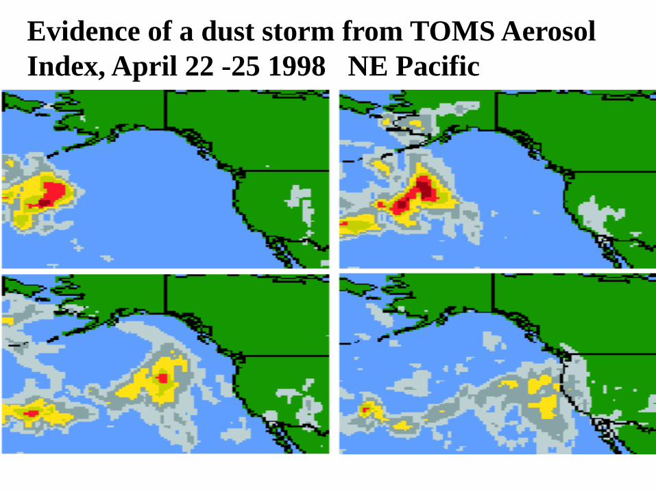
Evidence of a dust storm from TOMS Aerosol
Index, April 22 -25 1998 NE Pacific
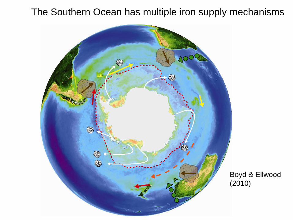
The Southern Ocean has multiple iron supply mechanisms
Boyd & Ellwood
(2010)

Upwelling of Iron
Cromwell undercurrent (Chavez et al. 1999)
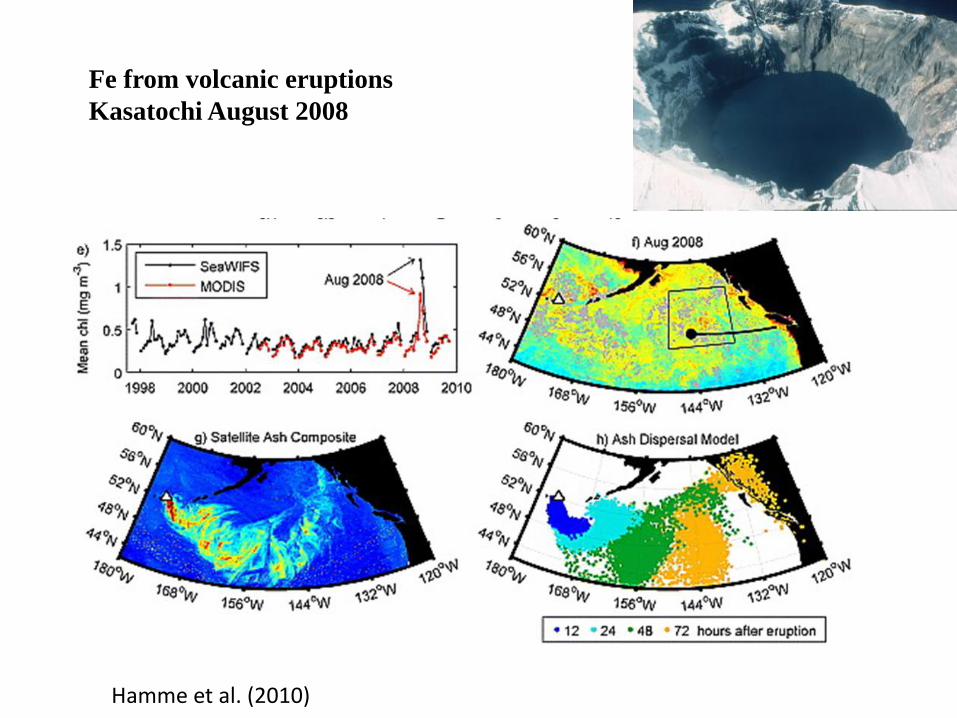
Fe from volcanic eruptions
Kasatochi August 2008
Hamme et al. (2010)

Offshore
movement of
Haida eddies
(containing high iron
levels) in the
Gulf of Alaska
(images Gower,
NASA)
0
1000
2000
3000
4000
5000
6000
0 2 4 6 8 10
Total Dissolvable-Fe conc. (nM)
Dep
t (m
)
C4
C1
C3
C2
C5
C7
C8
C9
C0
C10
KNOT
SEEDS
50ºN
45ºN
140ºE 145ºE 150ºE 155ºE 160ºE 165ºE
KNOT
C9
C10
C8
C7
C5
C2
C1 C3
C4 SEEDS
C0
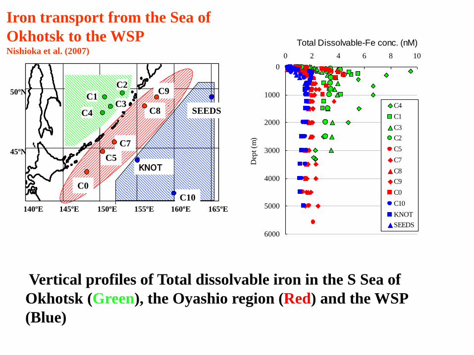
Vertical profiles of Total dissolvable iron in the S Sea of
Okhotsk (Green), the Oyashio region (Red) and the WSP
(Blue)
Iron transport from the Sea of
Okhotsk to the WSP Nishioka et al. (2007)

Fe supply from recycling
“The picture that emerges is one of an extremely dynamic
trafficking in essential trace metals in sea water”
Morel and Price [2003]

fe ratio = new Fe / (new + regen Fe)
Boyd & Ellwood (2010)
fe ratio’s range from < 0.1 - >0.5
c.f. f ratios
Recycling supplies 40 to 90% of
iron to the biota
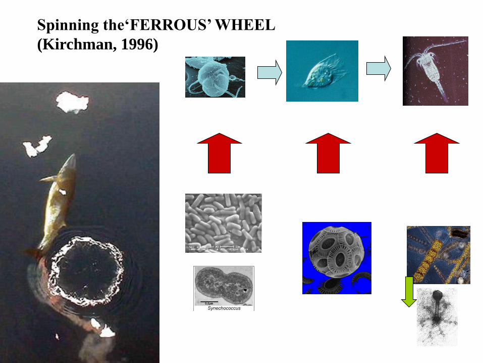
Spinning the‘FERROUS’ WHEEL
(Kirchman, 1996)

From Morel and Price [2003]
SINKS FOR Fe
Fe distributions
provide clues
as to the main
sinks for iron
Surface depletion
is indicative of biol.
uptake
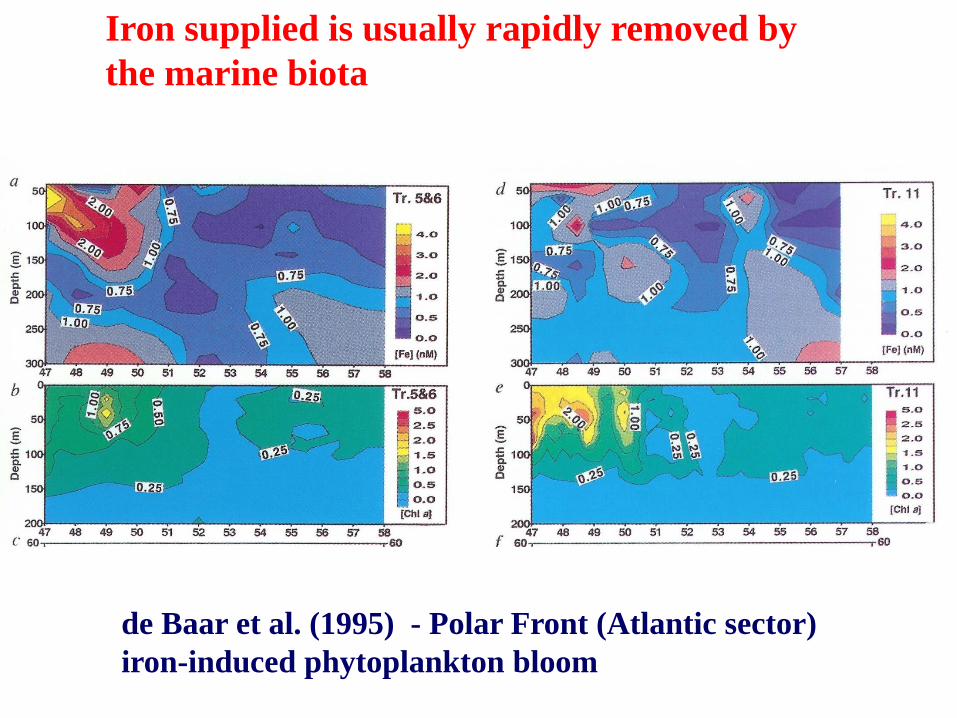
Iron supplied is usually rapidly removed by
the marine biota
de Baar et al. (1995) - Polar Front (Atlantic sector)
iron-induced phytoplankton bloom

0.1
0.15
0.2
0.25
0.3
0.35
0.4
0 2 4 6 8 10
Fragilariopsis kerguelensis
µ (
d-1
)
Fe dissolved (x10 -9 M )
Km Fediss: 0.44 x 10⁻⁹ M
µmax: 0.31 . d-1
Timmermans et al. [2004]
80 µm
Fragilariopsis kerguelensis
Iron uptake kinetics using natural
Antarctic seawater

IRON ACQUISITION STRATEGIES
Boyd & Ellwood (2010

DIFFERENT PHYTOPLANKTON
GROUPS HAVE DIFFERENT
IRON REQUIREMENTS
LOW
HIGH
??

Fe chemistry is complex!!
Algal
Cell
[Fe ] [Fe ]
[Fe(III)L] organic complexes
? ?
? ? photoreduction
sidero-
phores
PFe
Fe2O3
Fe(OH)3
FeOOH colloids
photoreduction
[Fe(OH) ] [Fe(OH) ] 2+
+
2 3+ 2+
[FeCO ] 0
3
[FeOH ] +
[Fe(II)L]?
(Courtesy of de Baar)
PHOTOCHEMISTRY
INTERACTIONS
WITH THE BIOTA

Forms of Iron
in Seawater
• Dissolved Colloidal Particulate
• Dissolved – two oxidation states - Fe(II) and Fe(III)
• Mainly present in non-reactive forms in the upper ocean
• Colloidal – poorly understood
• Particulate – biogenic, lithogenic, detrital
• Lithogenic iron present as oxyhydroxides, silicates and
aluminosilicates
• Fe silicates and aluminosilicates are mainly very unreactive
- contribute little to dissolved Fe in seawater and their fate
is governed by coagulation and settling processes
OH
OH
N
O
NN
NN
NN
NH2
OH OOH
O
O
HN
NH2HN
O
O
O
COOH
COOHHOHO COCH
H
H
H
H
H
H
H
(CH2)2 N
OH
C
O
CH3
CH2
NH
O
C
CH2
OH O
CH3CN(CH2)2
CH2
NH
O
CO2HHO C
C
CH2
C.
B.
A.
NH
O
HO OH
NH
O
NH2
O
O
HOO
N
O
HN O
HNOH
OHOON
NHO
O
N NH2
NH
HO
HO
H
H
H

Fe II and III - the redox cycle of Fe
The relative proportions of Fe(II) and Fe(III) in DFe in surface seawater
depend on the relative rates of reduction and oxidation
In well-oxygenated seawater Fe(III) is the thermodynamically stable form
Fe(II) is relatively soluble in seawater, Fe(III) is less so
Fe(II) is primarily produced photochemically and biologically, and is
rapidly reoxidised to dissolved Fe(III)
Fe(III) may be converted to Fe(II) by reductive processes including
photochemical, enzymatic, within micro-environments, & the formation of Fe(II)
organic complexes
Fe(II) Fe(III)
oxidation
reduction

Why is DFe so
unreactive?
• More than 99.999% of dissolved iron in
seawater is organically bound (Rue & Bruland,
1995)
• Fe(III) forms extremely strong organic complexes
• Upon addition of 7 nmol L-1 Fe (III) to seawater, >
50% was complexed to a strong ligand within 2
minutes (Wu and Luther, 1995)
• These organic complexes are referred to as iron-
binding ligands
OH
OH
N
O
NN
NN
NN
NH2
OH OOH
O
O
HN
NH2HN
O
O
O
COOH
COOHHOHO COCH
H
H
H
H
H
H
H
(CH2)2 N
OH
C
O
CH3
CH2
NH
O
C
CH2
OH O
CH3CN(CH2)2
CH2
NH
O
CO2HHO C
C
CH2
C.
B.
A.
NH
O
HO OH
NH
O
NH2
O
O
HOO
N
O
HN O
HNOH
OHOON
NHO
O
N NH2
NH
HO
HO
H
H
H

WHAT IS A LIGAND ?
The binding strength is measured electrochemically
and referred to as the
Conditional stability constant
So far two classes of iron-binding ligands
L1 or strong binding class [K FeL1, Fe(III)1 = 1013 L mol-1]
L2 or weaker ligand class [K FeL2, Fe(III)1 = 1011.5 L mol-1]
Ligands are molecules
characterised by high
binding strength
L1 are probably siderophores
L2 are released during particle breakdown (Boyd et al. 2010)
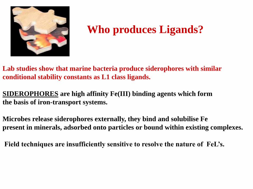
Who produces Ligands?
Lab studies show that marine bacteria produce siderophores with similar
conditional stability constants as L1 class ligands.
SIDEROPHORES are high affinity Fe(III) binding agents which form
the basis of iron-transport systems.
Microbes release siderophores externally, they bind and solubilise Fe
present in minerals, adsorbed onto particles or bound within existing complexes.
Field techniques are insufficiently sensitive to resolve the nature of FeL’s.

Case Study I
MESOSCALE IRON ENRICHMENTS
Boyd et al.
(2007)
SOLAS has conducted several major
Iron biogeochemical studies

50.1
50.12
50.14
50.16
50.18
50.2
50.22
-144.83 -144.80 -144.77 -144.74 -144.71
Long
Lat
-4.00 -2.00 0.00 2.00
-8.00
-6.00
-4.00
-2.00
0.00
2.00
4.00
C67
C68
C69
Iron is added to
the ocean along with
the tracer SF6
An initial area of
70 km2 is enriched
with Iron The formation of
a coherent
patch of high
SF6 is used to
track the
enriched waters
for weeks

The resulting bloom was large
enough to be viewed from space
The bloom as it develops
provides a laboratory to study
concurrent changes in physical,
chemical and biological signals
including climate-reactive gases
SERIES

10 15 20 25 30 35
mm
ol m
-2
0
100
200
300
400
500
Y A
xis
2
0
20
40
60
80
100
120
140
160
Days
DIFFERENT MICROBES
DOMINATE EACH PHASE OF
THE SERIES BLOOM
[POC]

Blooms and gas production /consumption Different groups influence gas concentrations in seawater
Direct Greenhouse
Stratospheric ozone
Tropospheric ozone
Sulfate
Fossil fuel soot
Biomass burning
Indirect tropospheric (CCN)
Solar
-2
-1
0
1
2
3
Glo
bal m
ean r
adia
tive f
orc
ing /
W m
-2
INDIRECT GREENHOUSE
DIRECT TROPOSPHERIC AEROSOLCO2
CH4
N2O
Halocarbon
CCN
Comparison of radiative forcing IPCC (1996)

CO2 and bloom development
Phytoplankton fix carbon
A small but significant
proportion of this C
settles out of the surface
ocean
To restore equilibrium
CO2 is drawn down into
the ocean

-40 -35 -30 -25 -20 -15 -10 -5 0 5
-10
-5
0
5
10
15
20
25
270
280
290
300
310
320
330
340
350
fCO2 (D18)
CO2 drawdown over
> 1000 km2
SERIES bloom

Chlorophyll (mg m-3)
Bloom
day 19
day 24
BLOOM DECLINE
CAN TAKE PLACE
VERY RAPIDLY
Boyd et al.
[2004]
7% of the
algal bloom
C was exported
to 125 m depth

Case Study II
Fe Biogeochemistry in HNLC waters
using the SF6 tracer – FeCycle
Boyd et al.
[2005]

Croot et al.
(2007)

20 40 60 80 100 120 140 160 180 200 220 240
-60
-40
-20
-100
1
3
5
10
25
50
100
200
300
400
500
600
700
800
900
SF6
Log SF6
-0.3
0.3
0.6
0.9
1.2
1.5
1.8
2.1
2.4
2.7
20 40 60 80 100 120 140 160 180 200 220 240
-60
-40
-20
Boyd et al. (2005)
Vertical & lateral iron supply terms from SF6
hours

Vertical
Diffusivity
PFe Export
Aeolian
Lateral
advection Biological
recycling
Mixed layer
Kilometers-10 -5 0 5 10 15
-10
-5
0
5
10
15
0
0.1
0.2
0.3
0.4
0.5
0.6
0.7
0.8
0.9
1
Fluxes measured during FeCycle

Iron uptake & recycling
Boyd & Ellwood (2010

A
Fe uptake (nmol l-1 d-1)
0.00 0.05 0.10 0.15 0.20
Dep
th (
m)
0
10
20
30
40
50
total
> 20 µm5-20 µm2-5 µm0.2 - 2 µm
B
0.00 0.05 0.10 0.15 0.200
10
20
30
40
50
C
0.00 0.05 0.10 0.15 0.200
10
20
30
40
50
D
0.00 0.05 0.10 0.15 0.200
10
20
30
40
50
McKay et al.
(2005)

Vertical
Diffusivity (g)
15+3
PFe Export (h)
216+27 to 548+128
Aeolian
500 (a)
5 to 50 DFe (b) [9 µmol m-2]
450 to 495 PFe (c) [34 µmol m-2]
>1976 (f) 0 (d)
2453 to 4055 (e)
Lateral
advection Biological
recycling
Mixed layer
Boyd et al. (2005) i.e. a fe ratio of < 0.1
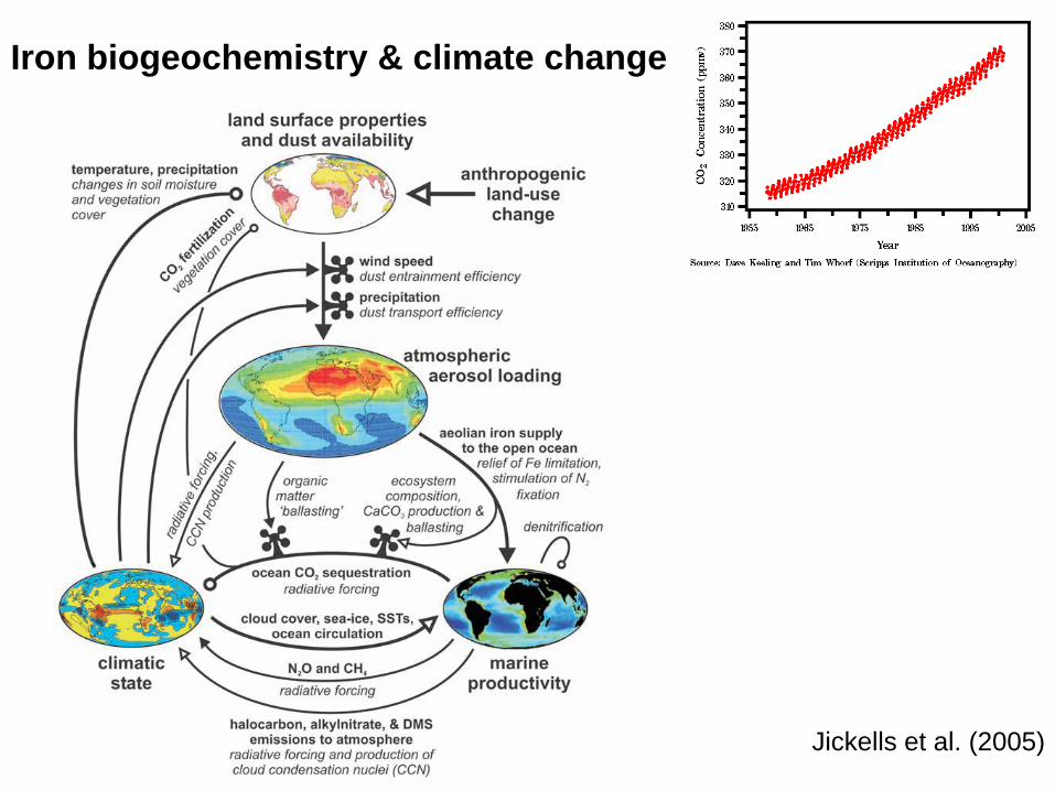
Iron biogeochemistry & climate change
Jickells et al. (2005)

ODP (red) & EPICA (black) dust and iron deposition records correspond
Large-scale changes in deposition i.e. most of the Southern Ocean
Suggests a CO2 drawdown of < 40 ppm from subantarctic iron fertilization
Stop press

How will these multiple supply mechanisms be altered?
Boyd & Ellwood
(2010)

Is a rapidly emerging field (SOLAS; GEOTRACES)
Adding iron to the oceans continues to attract commercial interest
and remains controversial
The impact of climate change on iron supply has many unknowns
New approaches such as iron stable isotopes hold great promise
IRON BIOGEOCHEMISTRY
Conclusions