BIOC 2005 Lab: From CEL Files to Annotated Listsof Interesting Genes

James W. MacDonald and Rafael A. Irizarry

August 13, 2005

1 Introduction

The predominant use for microarrays is the measurement of genome-wide expressionlevels, and the most commonly used microarray platform is the Affymetrix GeneChip.Affymetrix GeneChip arrays use short oligonucleotides to probe for genes in an RNAsample. Genes are represented by a set of oligonucleotide probes each with a lengthof 25 bases. Because of their short length, multiple probes are used to improve speci-ficity. Affymetrix arrays typically use between 11 and 20 probe pairs, referred to asa probeset, for each gene. One component of these pairs is referred to as a perfectmatch probe (PM) and is designed to hybridize only with transcripts from the intendedgene (specific hybridization). However, hybridization to the PM probes by other mRNAspecies (non-specific hybridization) is unavoidable. Therefore, the observed intensitiesneed to be adjusted to be accurately quantified. The other component of a probe pair,the mismatch probe (MM), is constructed with the intention of measuring only the non-specific component of the corresponding PM probe. Affymetrix’s strategy is to makeMM probes identical to their PM counterpart except that the 13-th base is exchangedwith its complement.

The identification of genes that are differentially expressed in two populations is apopular application of Affymetrix GeneChip technology. Due to the cost of this tech-nology, experiments using a small number of arrays are common. A situation we oftensee is the case where three arrays are used for each population. In this lab, we givean example of how to quickly create lists of genes that are interesting in the sense thatthey appear to be differentially expressed, starting from the raw probe level data (CELfiles). In Section 2, we briefly describe the functions necessary to import the data intoBioconductor. In Section 3 we talk about preprocessing. In Section 4, we describe waysto rank genes and decide on a cutoff. Finally, in Section 5 we describe how to makeannotated reports and examine the PubMed literature related to the genes in our list.

1

2 Reading CEL files

The affy package is needed to import the data into Bioconductor.

> library("affy")

In the Affymetrix system, the raw image data are stored in so-called DAT files. Currently,Bioconductor software does not handle the image data, and the starting point for mostanalyses are the CEL files. These are the result of processing the DAT files usingAffymetrix software to produce estimated probe intensity values. Each CEL file containsdata on the intensity at each probe on the GeneChip, as well as some other quantities.

To import CEL file data into the Bioconductor system, we use the ReadAffy function.A typical invocation is:

> library("affy")

> Data <- ReadAffy()

which will attempt to read all the CEL files in the current working directory and placethe probe-level data in an AffyBatch. If only a portion of the CEL files are to be read,one can use the filenames argument to select those files by name, or set the widget toTRUE to use a graphical user interface to select files. In this lab, we will not read in thedata. Instead we use an already created AffyBatch object, named spikein95, availablethrough the package SpikeInSubset.

> library("SpikeInSubset")

> data(spikein95)

An AffyBatch contains several slots that hold various data:

> slotNames(spikein95)

[1] "cdfName" "nrow" "ncol" "exprs"

[5] "se.exprs" "phenoData" "description" "annotation"

[9] "notes"

The cdfName slot contains the name of the Chip Description File, which maps the probesto their physical location on the chip, the nrow and ncol slots which give the dimensionsof the chip, the exprs slot which contains the probe level data (the se.exprs is not usedat this time), the phenoData slot which contains phenotypic data that describe eachsample, the annotation slot which contains the name of the annotation package for thechip, the description slot which contains the ’MIAME’ information for the experiment(see ?MIAME for more information), and the notes slot, which contains any notes aboutthe experiment.

The spikein95 Affybatch contains data from a six array subset (2 sets of tripli-cates) from a calibration experiment performed by Affymetrix. For the purpose of thisexperiment, we replace the current phenoData, describing the calibration experiment,with information needed for our example dealing with two populations.

2

> pd <- data.frame(population = c(1, 1, 1, 2, 2, 2), replicate = c(1,

+ 2, 3, 1, 2, 3))

> rownames(pd) <- sampleNames(spikein95)

> vl <- list(population = "1 is control, 2 is treatment",

+ replicate = "arbitrary numbering")

> phenoData(spikein95) <- new("phenoData", pData = pd,

+ varLabels = vl)

The assignment to phenoData above, can also be done using the function read.phenoData.There are various accessor functions available for extracting data from an AffyBatch.

Two notable examples are the pm and mm functions which are used to extract the PMand MM probe intensities. One may also pass a vector of Affymetrix probe IDs as thesecond argument to these functions to return intensities for only certain probesets. Moreinformation about the AffyBatch class can be found in the help page (accessed by typingclass ?Affybatch at an R prompt).

2.1 Quality Control

Obtaining gene expression measures for biological samples from Affymetrix GeneChipmicroarrays is an elaborate process with many potential sources of variation. In addition,the process is both costly and time consuming. Therefore, it is critical to make the bestuse of the information produced by the arrays, and to ascertain the quality of thisinformation. Unfortunately, data quality assessment is complicated by the sheer volumeof data involved and by the many processing steps required to produce the expressionmeasures for each array. Furthermore, quality is a term which has some dependency oncontext to which it is applied. From the viewpoint of a user of GeneChip expressionvalues, lower variability data, with all other things being equal, should be judged to beof higher quality.

There are several Bioconductor packages designed for the analysis of AffymetrixGeneChip data, each of which has a set of functions that can be used to assess overallquality of the raw data. The affy package supplies several functions for exploratorydata analysis (EDA), which is often the most powerful way to detect either outlier orhigh-variability chips.

> library("ALLMLL")

> data(MLL.B)

> Data <- MLL.B[, c(2, 1, 3:5, 14, 6, 13)]

> sampleNames(Data) <- letters[1:8]

> rm(MLL.B)

> gc()

Exercise 1The ALLMLL contains a subset of data from a large acute lymphoblastic leukemia (ALL)

3

study (Ross et al., 2004). The above code loaded the package and subsetted the resultingAffyBatch to contain just eight samples.

• Using the image function, plot a false color image of the first chip. Notice theobvious spatial artifact.

• Using the hist function, plot smoothed densities for each chip. Note the bimodaldistribution of the first chip - this is due to the spatial artifact noted above.

• Look at a boxplot of the chips - the high background of the ’f’ chip is obvious inthis plot.

3 Preprocessing

After checking overall chip quality, the next step is to preprocess the data to obtainexpression measures for each gene on each array. Preprocessing Affymetrix expressionarrays usually involves three steps: background adjustment, normalization, and summa-rization.

There are several methods available from Bioconductor for preprocessing AffymetrixGeneChip data. These methods include the mas5 function, which very closely duplicatesthe MAS5 method developed by Affymetrix (Affymetrix), the fit.li.wong function, whichemulates the MBEI method (Li and Wong, 2001), the rma function (Irizarry et al., 2003),and gcrma (Wu et al., 2005). In addition, the expresso function can be used to combinevarious background adjustment, normalization, and summarization methods.

Here we simply use rma to compute expression measures.

> eset <- rma(spikein95)

The rma function will background correct, normalize, and summarize the probe leveldata, as described by Irizarry et al. (2003), into expression level data. The expressionvalues are in log base 2 scale. The information is saved in an instance of the exprSet

class, which contains similar information to the AffyBatch class. Specifically, the ex-

prSet contains expression level as opposed to probe level data.A matrix with the expression information is readily available. The following code

extracts the expression data and demonstrates the dimensions of the matrix storing thedata:

> e <- exprs(eset)

> dim(e)

[1] 12626 6

4

We can see that in this matrix, rows represent genes and columns represent arrays. Toknow which columns go with what population, we can rely on the phenoData informationinherited from spikein95.

> pData(eset)

population replicate

1521a99hpp_av06 1 1

1532a99hpp_av04 1 2

2353a99hpp_av08 1 3

1521b99hpp_av06 2 1

1532b99hpp_av04 2 2

2353b99hpp_av08r 2 3

We can conveniently use $ to access each column and create indexes denoting whichcolumns represent each population:

> Index1 <- which(eset$population == 1)

> Index2 <- which(eset$population == 2)

We will use this information in the next section.As mentioned above, we are only demonstrating the use of RMA. Other options are

available through the functions mas5 and expresso. If you find expresso too slow, thepackage affyPLM provides an alternative, threestep, that is faster owing to use of Ccode.

Exercise 2• Compute expression values for these data using the mas5 function. Compare the

first replicate from the two populations using an ’M vs A’ plot (see ?mva.plot)Hint: you will need to subset out the two chips you want to compare. How doesthis compare to an M vs A plot for the same two samples using the rma expressionmeasure?

• The rma function fits a robust model to the data. As with all models, it is usefulto look at the residuals to see how well the model fits the data. Using the affyPLMpackage, compute rma expression measures and then plot residuals for each chip.Hint: see ?rmaPLM and the“Fitting Probe Level Models”vignette in the affyPLMpackage.

4 Ranking and filtering genes

Now we have, in e, a measurement xijk of log (base 2) expression from each gene j oneach array i for both populations k = 1, 2. For ranking purposes, it is convenient to

5

quantify the average level of differential expression for each gene. A naive first choice isto simply consider the average log fold-change:

dj = x̄j2 − x̄j1

with

x̄j2 = (x1j2 + x2j2 + x3j2)/3 and x̄j1 = (x1j1 + x2j1 + x3j1)/3, for j = 1, . . . , J.

To obtain d, we can use the rowMeans function, which provides a much faster alternativeto the commonly used function apply :

> d <- rowMeans(e[, Index2]) - rowMeans(e[, Index1])

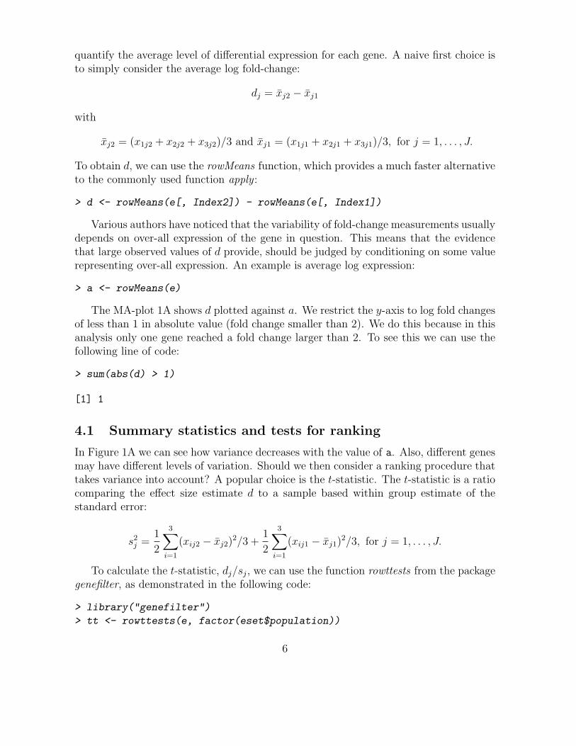
Various authors have noticed that the variability of fold-change measurements usuallydepends on over-all expression of the gene in question. This means that the evidencethat large observed values of d provide, should be judged by conditioning on some valuerepresenting over-all expression. An example is average log expression:

> a <- rowMeans(e)

The MA-plot 1A shows d plotted against a. We restrict the y-axis to log fold changesof less than 1 in absolute value (fold change smaller than 2). We do this because in thisanalysis only one gene reached a fold change larger than 2. To see this we can use thefollowing line of code:

> sum(abs(d) > 1)

[1] 1

4.1 Summary statistics and tests for ranking

In Figure 1A we can see how variance decreases with the value of a. Also, different genesmay have different levels of variation. Should we then consider a ranking procedure thattakes variance into account? A popular choice is the t-statistic. The t-statistic is a ratiocomparing the effect size estimate d to a sample based within group estimate of thestandard error:

s2j =

1

2

3∑i=1

(xij2 − x̄j2)2/3 +

1

2

3∑i=1

(xij1 − x̄j1)2/3, for j = 1, . . . , J.

To calculate the t-statistic, dj/sj, we can use the function rowttests from the packagegenefilter, as demonstrated in the following code:

> library("genefilter")

> tt <- rowttests(e, factor(eset$population))

6

The first argument is the data matrix, the second indicates the two groups being com-pared.

Do our rankings change much if we use the t-statistic instead of average log foldchange? The volcano plot is a useful way to see both these quantities simultaneously.This figure plots p-values (more specifically − log10 the p-value) versus effect size. Forsimplicity we assume the t-statistic follows a t-distribution. To create a volcano plot,seen in Figure 1B, we can use the following simple code:

This Figure demonstrates that the t-test and the average log fold change give usdifferent answers.

7

2 4 6 8 10 12 14

−1.

0−

0.5

0.0

0.5

1.0

A) MA−plot

a

d

●●

●

●

●

●●●●●●

●

●●

●

●

●●

●

●

●

●●

●

●●

●

●

●

●

●●●

●

●

●

●

●

●

●

●

●

●●

●

●

●

●

●

●

●

●

●

●

●

●

●

●

●

●

●

●

●●

●

●

●

●

●

●

●

●

●

●

●

●

●

●

●

●

●

●

●

●

●

●

●●

●

●

●

●

●

●

●

●●

●

●

●●

●

●

●

●

●

●

●

●

●●

●

●●

●●

●

●●

●

●

●●

●

●●

●

●

●

●●

●

●

●

●

●

●

●

●●●

●

●●

●

●

●

●

●

●

●

●

●

●

●

●

●

●

●●

●

●

●●

●

●

●

●

●

●

●

●

●●●

●

●●

●●

●

●●

●

●

●

●

●

●

●

●

●

●

●

●

●

●

●

●●●

●●●

●

●●

●

●

●

●

●

●

●

●

●

●●

●

●●

●

●●●

●

●●

●

●

●

●●

●

●●●

●

●

●

●

●

●

●

●

●

●●

●

●

●

●

●

●

●

●

●

●

●

●

●

●

●

●

●

●

●

●

●

●

●

●

●

●

●

●

●●

●

●

●

●

●

●

●

●

●

●●

●

●

●●

●

●

●

●

●

●●

●

●

●

●

●●

●

●

●

●

●

●

●

●

●

●

●

●●

●

●

●

●●

●

●

●

●

●

●

●●

●

●

●

●●

●

●●

●●●●

●

●

●

●

●●

●●

●

●

●●●

●

●●

●

●

●

●

●

●●

●

●

●

●

●●

●●

●●

●

●

●

●

●● ●

●

●

●

●

●

●

●●

●

●

●

●

●●

●

●

●

●

●

●

●●

●●

●●

●●

●

●

●

●

●

●●

●

●●

●●

●

●●

●

●

●

●

●

●

●

●●

●

●

●

●

●

●

●

●

●

●

●●

●

●

●

●

●

●

●

●

●

●

●●

●

●

●

●●●

●

●

●

●

●●●

●

●

●

●

●

●

●

●

●

●

●●

●

●

●

●●

●

●●

●

●

●

●

●

●

●

●

●

●

●●

●

●

●●

●

●

●

●

●

●

●

●

●

●●

●

●

●

●

●

●

●

●●

●

●

●

●

●

●

●

●

●●

●

●

●

●

●

●

●

●●

●

●

●●

●

●

●

●

●

● ●●

●

●

●

●

●

●

●●

●

●●

●

●

●

●

●

●

●

●

●

●

●●

●

●

●

● ●

●

●

●

●

●

●

●

●

●

●

●

●

●

●

●●

●

●

●

●

●●●

●●

●

●

●

●

●

●

●

●

●●

●●

●

●●●

●●

●

●

●

●

●

●

●

●

●

●

●

●

●

●●

●

●●

●

●

●●●

●

●●

●

●

●

●

●

●

●

●

●

●

●

●●

●

●

●

●

●

●

●

●●

●

●●

●

●

●

●

●

●

●

●

●

●

●●●

●

●

●●

●

●●

●

●

●

●

●

●

●

●●

●

●

●

●●

●

●●

●

●

●

●

●●

●

●

●

●

●

●

●

●

●

●●

●

●

●

●

●●

●

●

●

●

●

●

●●

●

●

●●

●

●

●

●

●●

●

●

●

●●

●

●

●● ●

●

●

●

●

●

●

●

●

●

●

●

●

●

●

●

●

● ●

●

●

●

●

●

●●

●

●●

●●

●

●

● ●

●

●●●

●

●

●

●

●

●

●

●

●

●●●

●

●

●

●

●●

●

●

●●

●

●

●

●

●

●

●● ●

●

●

●

●●

●●

●

●

●●

●

●

●

●●

●

●●

●●●

●

●

●●

●

●

●

●●

●

●

●

●●●

●

●●

●

●

●

●

●

●

●

●●

●

●

●●

●

●

●

●

●

●

●

●●

●

●

●●

●●

●

●

●

●

●

●

●●

●

●

●

●

●

●

●

●

●●

●●

●

●

●

●

●

●

●

●

●

●

●

●

●

●

●

●

●●

●

●

●

●

●● ●

●

●

●

●

●●

●

●

●

●

●●

●

●●

●

●●

●

●

●

●

●

●

●●

●

●●

●

●●●

●

●

●

●

●●

●

●●

●

●

●●

●

●

●●

●●

●

●

●

●●●

●

●

●

●●

●

●

●

●●

●●

●

●

●

●

●

●

●

●●

●

●●●

● ●

●●

●

●

●

●

●

●

●

●

●●

●●

●

●

●●

●

●

●

●

●

●

●●

●

●●

●

● ●

●

●

●

●

●

●

●

●●

●

●

●

●

●

●

●

●●●●

●

●

●

●

●

●

●

●

● ●

●

●

●

●

●

●●

●

●●●●

●

●●

● ●

●●

●

●●

●

●

●

●

●

●

●

●

●

●

●

●

●

●

●

●

●

●

●

●

●

●●

●

●

●

●

●

●

●●

●

●●●

●

●

●

●

●

●●

●

●●●

●

●

●

●●● ●

●

●

●●●

●

●

● ●

●

●

●

●

●

●

●

●●

●

● ●

●

●●●

●

●

●

●

●

●

●

●●

●●

●

●

●

●

●

●

●

●

●

●

●

●

●

●

●

●

●

●

●

●

●

●

●

●

●

●

●

●

●●

●●

●

●

●●

●

●

●

●

●●

●

●

●

●

●

●

●

●

●●

●

●

● ●●

●

●

●●

●

●

●

●

●●

●●

●●

●

●

●

●

●

●●

●

●

●

●

●

●

●

●

●

●

●

●

●

●●

●

●

●

●

●

●

●

●

●

●

●

●

●

●

●

●

●

●

●

●

●

●●

●

●●

●●

●

●

●

●

●

●

●

●

●

●

●

●

●

●

●

●

●

●●●

●

●

●

●

●

●

●●●

●●

●

●●

●

●

●

●

● ●

●

●

●

●

●

●

●

●

●

●

●

●

●

●

●●

●

●●

●

●●

●

●

●

●

●●

●

●

●

●●

●

●●

●

●

●

●●●

●

●

●●

●●

●

●

●

●●

●

●

●

●

●

●

●

●

●

●●

●

●

●

●●

●

●

●

●

●

●

●●●●

●

●

●

●

●●

●

●

●●

●

● ●

●

●

●

●

●

●

●●

●●● ●

●

●

●

●

●

●

●

●

●

●

●

●

●

●

●

●●

●●

●

●

●

●

●●

●●●

●

●

●

●

●

●

●●

●

●

●

●

●

●

●

●

●●

●

●

●

●

●

●

●

●●●

●

●

●

●

●

●

●

●

●

●

●●●

●

●

●

●

●

●

●

●

●

●

●

●

●

●

●

●

●

●

●

●

●

●

●

●

●

●

●

●

●

●

●

●

●●

●

●

●●

●

●

●●

●

●

●

●

● ●●

●●

●

●

●

●

●

●

●

●

●

●

●

●●

●

●

●

●

●

●

●●

●

●

●

●●

●

●

●

●

●

●

●

●

●

●●●

●

●

●

●

●

●

●

●●

●●

● ●

●●

●

● ●

●

●

●●

●

●

●

●

●

●

●

●

●

●

●

●

●

●

●

●●

●

●

●

●

●

●

●●

●

●

●

●

●

●

●●●

●

●

●

●

●

●

●

●

●

●

●

●

●●

●

●

●

●

●●

●

●

●●

●

●

●

●

●

●

●

●

●

●

●

●●

●

●

●

●

●

●

●

●

●

●●

●

●

●

●●

●

●●

●

●

●

●

●●

●

●

●

●● ●

●

●

●

●

●

●●

●

●

●

●

●

●

● ●

●

●

●

●●

●

●

●

●●

●

●

●

●

●

●

●

●●

●

●

●

●

●

●

●

●

●

●

●

●●

●

●

●

●

●

●

●

●

●

●

●

●

●

●

●

●

●

●

●

●●

●

●

●

●

●●

●

●

●

●●

●●●

●●

●

●

●

●

●

●

●

●

●

●

●

●●

●

●

●

●

●

●

●

●

●

●

●

●

●●

●

●

●

●

●

●

●

●●

●

● ●●

●

●

●

●

●●

●

●●

●

●

●

●

●

●

●

●

●

●

●

●

●

●

●

●

●

●

●

●

●

●

●

●

●●

●

●

●

●●●

●

●

●●

●

●

●

●

●● ●

●

●

●

●

●

●

●●●

●

●

●

●

●

●

●

●

●

●

●

●●●

●

●

●

●

●

●

●

●

●

●●

●●●

●

●

●

●

●

●

●●

●

●

●

●

●

●

●

●

●

●

●●

●

●

●

●

●

●

●

●

●

●●

●

●

●

●

●

● ●

●

●

●

●

●

●

●

●

●

●

●

●●

●

●

●

●

●

●

●

●

●

●

●

●●

●●

●

●

●●

●

●

●●

●

●

●●

●

●

●

●●

●

●

●●

●

●

●

●

●

●

●

●

●

●

●

●

●

●

●

●

●

●

●●

●

●

●

●

●●

●●

●

●

●

●●

●

●

●

●

●

●

●

●

●

●●

● ●●

●

●

●

●

●

●

●

●

●

●

●●

●●

●

●

●

●

●●

●

●

●

●

●●

●

●

●

● ●

●

●

●

●●

●

●●●

●

●

●

●

●

●

●

●

● ●

●

●

●

●

●●

●

●

●

●

●

●

●

●

●●●

●

●

● ●

●

●

●

●

●

●

●

●

●

●

●

●

●

●

●

●

●

●

●

●

●

●

●

●

●●

●

●●

●

●●

●

●

●

●

●●●

●

●● ●

●●

●

●

●

●

●

●

●

●●

●

●

●

●

●

●● ●

●

●

●

●

●

●

●

●

●

●

●

●

●

●

●

●

●

●

●

●●

●

●

●

●

●

●

●

●

●

●●●

●

● ●

●

●●●

●

●

●

●

●

●

●

●

●

●●

●●

●

● ●●

●

●

● ●

●

●●

●

●

●

●●

●

●

●

●

●

●

●

●

●

●

●

●

●

●

●

●

●

●

●●●

●

●●

●

●

●

●

● ●

●

●

●

●

●●

●

●

●

●

●

●

●

●

●●

●

●

● ●

●

●

●

●

●

●

●

●

●●

●

●

●

●

●

●●

●

●

●

●

●

●●

●

●

●

●

●●●

●

● ●

●

●

●

●

●

●

●

●

●●

●●

●

●

●

●

●

● ●

●●

●

●

●●●

●

●●

●

●

●

●

●

●●

●

●

●

●

●

●

●

●

●

●

●

●

●●●

●

●

●

●

●

●

●

●

●

●●

●●

●

●

●●

●

●●

●

●●

●●

●

●

●

●

●

●

●

●

●●

●

●

●

●●

●

●

●●

●

●

●●

●

●

●

●●

●

●

●

●

●

●●

●

●●

●

●

●●

●

●

●

●

●

●

●●

●●

●

●

●

●

●●●

●

●

●

●●

●●

●

●

●

●

●

●

●

●●

●

●

●

●

●●

●

●●

●

●●

●

●●

●

●

●

●●●●

●

●

●

●

●

●●●

●

●

●●

●

●

●

●

●●

●

●

●

●

●

●

● ●

●

●

●●●

●

●●

●

●

●

●

●

●●

●

●●

●

●

●

●

●

●

●

●

●

●

●●

●

●●

●

●

●

●●

●

●

●●

●

●

●

●

●●

●

●

●

●

●

●●

●●

●

●

●

●

●●●

●

●●

●

●

●●

●

●

●

●

●

●●

●

●

●

●

●

●●

●

● ●●

●

●

●

●

●

●

●

●

●

●

●

●

●●

●

●

●

●

●

●

●

● ●

● ●

●

● ●

●

●

●

●

●

●

●

●

●●●

●

●

●

●●

●

●

●

●

●

●

●

●

●

●

●●

●

●

●●

●

●

●

● ●

●

●

●

●

●

●

●●

●

●

●

●●●

●

●

●

●

●

●●

●

●

●

●

●

●

●

●

●

●

●

●

●●

●●

●

●●●

●

●

●

●

●●

●

●

●

●

●

●

●

●

●

●

●●

●

●

●

●

●

●

●

●

●

●

●

●

●

●

●

●

●

●

●

●

●

●

●

●

●

●

●

●

●

●●

●●

●●

●

●●

●

●

● ●

●

●

●

●

●

●

●●

●

●

●

●

●

●

●

●●● ●

●

●

●

●

●

●●

●

●

●

●

●

●

●

●●

●●

●

●

●

●

●

●

●

● ●

●

●

●

●●

●

●

●

●

●

●

●

●

●

●

●

●

●

●

●●

●

●

●

●

●

●

●

●

●●

●

●

●

●

● ●

●

●

●●

●

●●

●●

●

●

●

●●

●

●

●

●●●

●

●● ●

●

●

●

●

●

●

●

●

●

●

●

●

●

●●

●●

●

● ●

●

●●●●

●● ●

●

●

●

●

●

●

●

●

●

●●

●

● ●●●

●

●

●

●

●●

●●

●

●

●●●

●

●

●

●

●

●

●

●

●

●

●

●●

●

●

●

●

●

●

●●

●

●

●●

●

●

●

●

●

●

●

●

●

●

●●

●

●

●

●

●

●

● ●

●

●

●

●●

●

●

●

●

●

●●

●●

●

●

●

●

●

●

●

●●

●

●

●

●

●●

●

●

●

●●

●

●

●

●

●

●

●

●

●

●

●

●

●

●

●

●●

●

●

●

●

●

●

●

●

●

●

●

●

●

●

●

●

●

●

●

●

●

●

●●

●

●

●

●

●

●●●

●●●

●

●

●

●

●●

●

●●

●●●

●

●

●

●

●

●

●

●

●

●

●●●●

●

●

●

●

●

●

●

●

●●●

●

●

●

●●●

●

●

●

●

●

●

●

●

●

●

●

●

●

●

●

●●

●

●

●

●●

●

●●

●

●●

●

●

●

●

●

●●

●

●

●

●●●

●

●

●

●

●●

●

●

●

●

●

●

●

●

●

●

●

●

●

●

●

●

●

●●

●●

●● ●

●

●

●

●

●

●

●

●

●

●

●●

●

●

●

●

●

●

●

●

●●

●

●

●

●

●

●

●

●●

●

●●

●

●

●

●

●

●

●●●

●●

●●

●

●●

●

●●

●

●

●

●

●●●

●

●

●

●

●

●

●

●

●

●

●

●

●●

●

●●

●

●●

●●

●

●

●

●●

●

● ●

●●

●

●

●

●

●●

●●

●

●

●

●●

●

●

●

●

●●

●

●

●

●

●

●

●●

●

●

● ●

●

●

●●

●

●

●

●

●

●

●

●

●

●

●

●

●

●●

●●●●

●

●

●

●

●●

●

●

●

●

●

●

●●●

●

●

●

●

●●

●

●●

●

●

●●

●

● ●

●

●

●

●

●

● ●

●

●●

●

●

●

●

●

●

●

●

●

●

●

●

●●

●

●

●

●

●●

●

●

●

●● ●

●

●

●

●●

●

●

●

●

●●

●

●

●●

●

●

●

●

●

●

●

●●

●

●

●

●●

●

●

●

●

●●

●

● ●●

●

●

●

●

●

●

●●

●

●

●

●

●

●

●

●

●●

●

●

●

●

●

●

●

●

●

●

●

●

●

●

●●

●

●

●

●

●

●

●

●

●

●

●

●

●

●

●

●

●●

●

●

●

●

●

●

●

●

●●

●

●

●

●

●

●

●

●

●●

●●

●

●

●

●●

●●

●

●

●●●

●●

●

●

●

●

●

●

●●

●

●●●

●

●

●

●

●

●

●

●

●

●

●●

●

●●

●

●

●

●●●

●

● ●

●

●

●

●

●

● ●

●

●

●

●

●

●

●●

●

●

●●

●

●

●

●●

●

●●

●

●●

●

●

●

●

●

●

●●●

●

●

●

●

●

●

●

●

●●

●

●

●

●

●

●

●

●

●

●

●

●●

●

●●

●●

●

●

●

●●

●

●

●●

●●

●

●

●●

●

●

●

●

●

●

●

●●

●●

●

●

●

● ●

●

●

●

●

●

●

●●●

●●

●

●

●

●●

●

●

●

●●

●

●

●

●

●

●●●●

●

●

●

●●

●

●

●

●

●

●

●

●

●●

●

●

●

●

●●

●

●

●

●

●

●

●

●

●

●

●

●●

●

●

●

●

●

●●

●

●

●

●●

●

●

●●

●

●

●●

●

●

●

●

●

●

●

●

●

●

●

●

●

●

●

●

●

●

●

●

●●

●

●

●

●

●

●●

●

●

●

●

●

●

●

●

●

●

●●

●

●

●

●

●

●

●

●

●

●●

●

●

●

●

●●

●

●●●

●

●

●

●

●

●

●

●●

●

●

●●●

●

●

●

●

●

●●

●●

●

●●

●

●

●●●

●●●

●

●

●

●

●

●

●

●

●●●

●●

●

●

●

●

●

●

●

●●

●

●

●●

●●

●

●

●

●

●

●●

●●●

●

●

●

●

●

●

●

●

●

●

●

●

●●

●●

●

●

●

●

●

●

●

●

●●

●

●

●

●

●●

●

●

●

●

●

●

●

●

●●

●

●

●

●●

●

●●

●

●

●

●

●

●

●

●

●

●

●

●

●

●●

●

●

●

●

●

●

●●

●

●

●

●

●

●●

●

●

●

●

●

●

●

●

●●

●

●●

●

●

●

●

●

●

●

●

●

●

●

●

●

●●

●

●●

●

● ●

●

●

●

●●

●

●●

●

●

●

●●

●

●

●

●

●

●

●

●●●

●●

●

●

●

●

●

●

●

●

●

●

●

●●

●

●

●

●

●

●

●

●

●

●

●●●

●

●

●

●●

●

●

●

● ●

●

●

●

●

●●

●

●

●

●

●

●

●

●

●

●

●●

●

●

●

●

●●

●

●

●●

●

●●

●●

●

●

●

● ●●

●●

●

●

●

●

●

●

●

●

●●

●

●●

●

●●

●

●

●

●

●

●

●

●

●

●

●●

●

●

●

●

●●●

●

●●

●

●

●

●

●

●

●

●

●

●

●●

●

●

●

●

●

●

●

●

●

●

●

●

●

●

●

●

●

●

●

●

●

●

●●

●

●

●

●

●●

●

●

●

●

●

●●

●

●

●

●

●

●●●●

●

●●

●

●

●

●

●

●

●

●

●●

●

●

●

●

●

●

●

●

●

●

●

●

●●

●

●

●

●●

●

●●

●

●

●

●

●

●

●

●

●

●

●

●

●

●

●

●

●

●●

●

●

● ●

●

●

●

●

●

●

●

●

●

●

●

●

●

●

●

●

●

●

●●

●

●

●

●

●

●

●

●●

●

●

●

●

●

●

●

●

●

●

●

●●

●

●

●

●

●

●

●

●

●

●

●

●

●

●

●

●●●●

●

●

●

●

●

●●●●

●

●●

●●

●●

●

●

●

●●

●

●

●

●●

●●

●●

●

●

●

●

●

●

●●

●

●

●

●

●

●

●

●

●

●

●

●

●

●

●

●

●

●

●

●

●

●

●

●●●

●

●

●

●

●

●

●●

●

●

●

●

●

●

●●

●●

●●●●

●

●

●●

●

●●

●

●

●●

●

●

●

●

●

●

●

●●

●

●

●●

●

●

●

●

●

●

●

●

●

●

●●

●

●

●

●

●

●

●

●

●

●●

●

●

●

●

●

●●

●

●

●

●

●

●

●●

●

●●

●

●●

●

●

●

●

●

●

●

●●

●

●

●

●●●

●

●

●

●

●

●

●

●

●

●

●

●

●●

●

●

●

●

●●

●

●●

●●

●

●●

●

●●●

●

●

●

●

●

●

●

●

●

●

●

●

●

●

●

●

●●

●●

●●

●

●

● ●

●

●

●●●

●

●

●

●

● ● ●

●●

● ●

●

●

●

●

●

●

●

●

●

●

●

●

●●

●

●

●

●

●

●

●

●

●

●●

●

●

●

●

●●●

●

●

●

● ●

●

●

●

●

●

●●

●

●

●

●●

●

●

●

●

●

●

●

●

●

●●

●

●

●

●

●

●●●

●

●

●

●

●

●●

●

●●

●●●

●

●

●

●

●

●

●

●

●

●

●

●

●

●

●

●

●

●

●

●●

●●

●●

●

●●

●

●

●

●

●

●

●●

●

●

●

●

●

●

●

●

●

●

●

●

●

●

●

●

●

●

●

●

●

●

●

●●

●

●

●●●

●

●

●

● ●

●

●

●

●

●●

●

●●

●

●

●●

●

●

●

●

●

●

●

●

●

●

●●

●

●

●

●●

●

●

●

●●

●

●

●

●●

●

●●

●

●

●

●

●

●

●

●

●●

●

●

●

●

●●

●

●

●

●

●

●

●

●●

●

●

●

●

●

●●

●

●

●

●

●●

●

●

●

●

●

●

●

●

●●

●

●

●

●

●

●

●●

●

●

●

●

●●

●

●

●

●

●●

●●●

●

●

●

●

●

●

●

●●

●

●

●

●

●

●

●

●

●

●

●

●

●

●●

●

●

●

●

●●

●

●

●

●

●

●

●

●

●

●

●

●

●

●

●

●

●

● ●

●

●●

●

●

●

●

●

●●

●

●●

●

●

●

●

●

●

●

●●

●

●

●

●

●

●

●

●

●

●

●

●

●

●

●●

●

● ●

●●

●●

●

●

●

●

●

●

●

●●●

●

●

●

●

●

●

●

●

●

●

●

●

●● ●

●

●

●●

●●

●●

●

●

●

●●●

●●

●

●

●

●

●●●

●●

●

●

●

●●

●

●

●

●

●

●

●

●

●

●

●

●

●

●●

●

●

●

●●

●

●

●

●

●

●

●●

●

●

●●

●

●●

●

●

●

●

● ●

●

●

●

●

●

●

●●

●

●

●

●

●

●

●

●

●●

●

●

●●

●●

●

●

●

●

●

●

●

●

●

●

●

●

●

●●

●

●

●

●

●

●

●●●

●

●

●

●

●●●

●

● ●●●

●

●

●

●

● ●

●

●

●

●●

●

●

●

●

●

●●

●

●

●

●

●

●

●

●

●

●

●●●

●

●

●

●

●

●

●●●

●

●

●

●

●

●●

●

●

●●

●

●

●

●

●

●

●

●●

●

●

● ●

●

●

●●

●

●

●●

●

●

●●

●

●

●

●

●

●

●

●

●

●

●

●

●

●

●

●●

●

●

●

●

●

●

●

●

●

●

●

●

●

●

●●

●

●

● ●

●

●

●

●

●●

●

●

●

●●

●

●

●

●

●

●

●

●

●

●

●

●

●

●●●

●

●●

●●●

●

●

●●

●

●●

●

●

●●

●

●●

●

●

●

●

●

●

●●

●●

●●

●

●

●●

●

●

●

●

●

●

●

●

●

●

●

●

●

●●

●

●

●

●

●●●

●

●

●

●●

●

●

●

●

●

●

●

●

●

●

●

●

●

●

●

●

●

●

●

●●

●

●

●

●

●●

●

●●

●

●

●

●●

●

●

●

●

●

●●

●●●

●●

●

●●

●

●

●

●

●

●

●●

●

●

●

●

●

●

●●

●

●

●●

●

●

●

●

●

●

●●

●

●

●

●

●

●

●

●

●

●

●

●

●

●

●

●

●●

●

●

●

●

●

●

●

●

●

●

●

●●

●●

●●

●●

●

●●●

●

●

●

●

●

●

●●

●

●

●

●

●

●

●●

●

●

●

●

●

●

●

●

●

●

●

●●

●

●

●

●

●●

●

●

●

●

●

●

●

●

●

●

●●

●

●

●

●

●●

●

●

●

●●

●

●

●

●●

●●

●

●

●●

●

●

●

●

●

●●●

●

●

● ●

●

●

●

●

●

●

●

●

●

●●

●

●●

●

●

●

●●

●

●

●

●●

●

●

●●

●

●

●

●

●

●●

●

●

●●

●

●

●

●

●

●

●

●

●

●●

●

●

●

●

●

●

●

●

●

●

●

●

●

●

●

●

●●●●

●

●

●

●

●●

●

●

●

●

●

●

●

●●

●

●

●

●

●

●

●

●

●

● ●

●

●

●

●

●

●

●

●

●

●

●●

●

●

● ●●

●

●

●

●●●

●

●

●

●

●

●

●

●

●

●

●●●

●

●

●

●

●

●

●

●●

●

●

●

●

●

●

●

●

●

●

●

●

●

●

●●

●

●●

●

●

●

●

●

●

●

●

●

●

●●

●

●

●

●●

●

●

●

●●

●

●

●

●

●

●

●

●

●

●

●

●

●

●●

●

●

●

●

●

●

●

●

●

●●

●

●

●●

●●

●

●

●●

●

●

●

●

●

●

●

●

●

●

●

●

●

●

●●●

●

●

●

●

●

●

●

●●

●

●

●●

●

●●

●●

●

●

●

●

●

●

●

●

●

●

●

●

●

●

●

●

●●

●

●

●●

●

●

●●

●

●●

●

●

●

●

●

●

●

●

●

●●

●

●

●●

●

●●

●

●

●●

●

●

●

●●

●●

●

●

●●

●

●

●

●

●●●

●●

●●

●

●

●

●

●

●

●

●

●●

●

●

●

●

●

●

●

●

●

●

●

●●

●

●

●●●

●●

●●

●

●

●●

●

●

●

●

●

●

●

●●

●●

●

●

●

●

●

●

●●

●

●

●

●

●●

●

●

●

●

●

●

●

●

●

●

●

●

●

●

●

●

●

●

●

●

●

●

●

●

●

●

●

●

●●

●

●●

●

●

●

●

●

●

●

●

●

● ●

●●

●

●

●

●

●

●

●

●

●

●

●

●

●

●

●

●●

●●

●

●

●●

●

●●

●

●

●

● ●

●●●

●

●●

●●

●

●

●

●

●

●

●

●●

●

●

●

●

●

●

●

●●

●

●

●

●

●

●

●

●

●

●

●

●

●

●

●

●

●

●

●

●

●

●

●

●

●

●

●●

●

●

●●

●

●

●

●

●

●●

●

●

●

●

●

●

●

●

●●

●

●

●

●

●

●

●

●

●

●●

●

●

●●

●

●

●

●

●

●

●

●

●●

●

●

●●

●

●

●

●

●

●

●

●

●

●

●

●

●

●

●

●

●

●

●●

●

●●

●●

●

●

●

●

●

●

●● ●

●

●

●

●

●

●

●

●

●

●

●

●●

●●

●

●

●

●

●

●●

●

●

●

●

●

●

●

●

●

●●

●●

●

●

●

●●●

●

●

●

●

●

●

●●

●

●

●

●

● ●

●●

●●

●●

●●

●

●

●

●

●

●

●

●

●

●

● ●

●

●

●

●

●

●

●

●

●

●

●●●

●

●

●●

●

●

●

●

●

●

●

●

●

●●

●

●

●

●

●●●

●

●

●

●

●

●

●●

●

●

●●

●●

●

●

●●

●

●

●

●

●

●

●

●

●

●

●

●●

●

●

●

●

●●

●

●

● ●

●●

●

●

●●

●

●●

●

●

●

●

●

●

●●

●●

●

●

●

●

●

●

●●

●

●

●

●

●

●

●

●

●

●

●

●●●

●

●

●

●

●

●

●

●●

●

●

●

●

●

●

●

●

●

●

●

●

●

●

●●

●●

●

●

●

●

●

●

●

●●

●

●

●

●

●

●

●

●

●

● ●

●

●●

●

●●●

●

●●

●

●

●

●

●

●

●

●

●

●

●●

●

●

●

●

●

●

●

●

●

●●●

●

●

●

●

●

●

●

●

●

●

●

●

●

●

●

●

●

●

●

●

●●

●●

●

●

●

●

●

●

●

●

●

●

●

●●

●

●

●

●●

●

●

●

●●

●

●

●

●

●

●

●

●

●

●

●

●

● ●●

●

●●

●

●

●

●

●

●

●

●

●

● ●

●

●

●

●

●

●

●

●

●●

●

●

●

●

● ●●

●

●

●

●

●

●●●

●

●

●

●

●

●

●

●●

●

●

●

●

●

●

●

●

●

●

●●

●

●

●●

●

●

●

●

●

●

●●

●

●

●

●●

●●

●

●

●

●

●

●

●

●

●

●

●

●

●

●

●

●

●●

●

●

●

●

●

●

●

●

●

●

●

●

●

●

●

●●●

●

●

●

●

●

●

●●

●

●

●

●

●

●

●

●

●

●

●

●

●

●

●

●

●

●

●

●

●

●●

●

●

●●

●

●

●

●

●

●

●

●●

●

●●●

●●

●●

●●●

●

●

●●

●●

●

●

●●

●

●

●

●

●

●

●

●

●

●

●

●

●

●

●

●

●

●

●

●●

●

●

●

●●

●●

●●

●

●●

●

●

●

●

●●

●

●

●

●●

●

●●

●

●●

●

●

●

●

●

●

●●

●

●

●

●

●

●

●

●●

●

●

●

●

●●

●

●

●

●

●●

●

●

●

●

●●

●

●

●

●

●

●

●

●

●

●

●●

●

●●

●

●●●

●

●

●

●

●●

●

●

●

●

●

●

●

●

●

●

●

●

●●

●

●

●

●

●

●

●

●●

●

●

●

●

●●

●

●●

●

●

●

●

●

●

●

●

●

●

●●

●

●

●

●

●

●

●●●

●

●

●

●●

●●

●

●

●●

●

●

●

●

● ●●

●

●●

●

●●●

●●●●

●●

●

●

●

●

●

●

●

●

●

●

●

●

●

●

●

●

●

●

●

●

●

●

●

●

●

●

●

●

●

●

●

●

●

●

●

●

●●●

●

●

●●

●

●

●

●

●

●

●

●

●●

●

●

●

●

●

●

●

●

●

●

●

●

●●

●

●

●

●

●

●

●●

●

●

●

●

●

●

●

●

●

●

●●●

●

●

●

●

●

●

●

●

●

●●

●

●

●

●

●

●

●

●

●

●

●

●

●

●●

●

●

●●

●

●

● ●

●

●

●

●●

●

●

●

●

●

●

●●

●

●●

● ●

●

●

●

●●

●●

●

●

●●

●

●

●

●

●

●

●

●

●

●

●●

●●

●

●

●

●●●

●

●

●

●

●

●

●●

●

●●

●

●

●

●●

●●

●

●

●

●

●

●

●

●

●

●

●

●

●

●●

●

●

●

●

●

●

●

●

●●

●

●

●

●

●

●

●

●

●

●

●

●

●

●●

●

●

●

●

●●

●

●

●

●

●●

●

●

●

●●

●

●●

●●

●●

●

●

●

●

●

●●

●

●

●

●

●●

●

●

●

●

●

●

●

●

●

●

●

●

●

●

●●

●

●●

●

●

●

●

●

●

●●

●

●

●

●

●

●●

●

●

●

●

●

●

●

●

●●

●

●

●

●

●

●

●

●

●

●●●●

●

●

●

●

●

●

●

●

●

●

●●

●

●

●

●

●

●

●

●

●●●

●

●

●●

●

●

●

●●

●

●

●

●

●

●

●●

●

●

●

●

●●

●●●●

●

●

●

●

●

●●

●●

●

●

●

●●

●●

●

●

●

●

●

●

● ●

●●

●

●

●

●●

●

●

●

●

●

●●

●

●

●

●

●

●

●●

●●●●

●

●

●

●

●●

●

●

●

●

●

●

●

●

●

●

●

●

●

●●

●●

●

●

●

●

●●

●

●

●

●

●

●

●

●●

●

●

●

●●●

●●

●

●

●

●

●

●

●

●●●

●●

●

●

●

●●

●

●

●

●

●●

●

●

●

●●

●

●●

●

●

●

●

●

●

●

●

●●●

●●●

●

●

●

●

●●

●

●

●

●

●

●

●

●

●

●

●

●

●

●●●

●

●

●

●

●

●●

●●●

●●

●

●

●

●

●

●●

●

●●

●

●

●

●

●●

●

●

●●

●

●

●

●

●

●

●

●

●

●

●

●●

●

●

●

●

●

●

●

●

●

●

●

●

●

●

●●

●

●

●

●

●

●

●

●

●

●●

●

●

●

●

●

●

●

●

●

●

●

●

●●

●

●

●

●

●

●

●

●

●

●●●

●●

●

●

●

●

●

●

●

●

●

●

●

●

●

●

●

●

●

●

●

●

●

●

●

●

●

●

●

●

●

●

●

●

●

●●●●

●

●

●

●

●

●

●

●●●

●

●

●

●

●

●

●●

●

●

●

●

●

●

●

●

●

●

●

●●

●

●

●

●

●

●

●

●●●

●

●

●

●

●

●

●

●

●

●

●

●

●

●

●

●

●

●

●

●●

●●

●

●

●

●●

●

●●

●

●

●

●

●

●

●●

●●

●

●

●●

●

●

●

●

●

●

●●

●

●

●

●

●

●●

●

●

●

●

●

●●

●

●●

●

●

●

●

●●●

●

●

●

●

●

●●

●

●●●

●

●

●

●

●

●

●

●

●

●

●

●

●

●

●

●

●

●

●

●●

●

●●

●

●

●

●

●

●

●●

●

●

●

●

●

●

●

●

●

●

●

●●●

●

●●

●

●

●

●

●

●

●

●

●●

●●

●

●

●

●

●●

●

●

●

●

●

●

●●

●

●

●

●

●

●

●●

●

●

●

●●

●

●

●

●

●

●

●

●

●●

●

●

●●

●

●

●

●

●

●

●

●

●

●

●

●

●

●

●

●

●

●●

●

●

●

●

●

●●

●

●

●

●

●

●

●●

●

●

●

●

●

●

●

●

●

●

●●

●

●

●

●

●

●●

●

●●●

●

●

●

●

●

●

●●●

●

●●●

●

●

●●

●

●

●

●

●

●

●●

●

●

●

●●

●

●

●

●

●

●

●●●

●

●●

●●●

●●

●

● ●

●

●

●●

●

●

●

●

●

●●

●

●●

●

●●

●

●

●● ●

●●

●

●●

●

●

●

●●

●●

●

●

●

●

●●

●

●

●

●

●

●

●

●

●

●

●

●

●

●

●

●

●

●

●

●●

● ●

●●

●

●

●

●

●

●● ●

●●

●●

●

●●

●

●

●

●

●

●

●

●

●

●

●

●

●●

●

●

●

●

●●

●●

●

●

●

●

●

●

●

●

●

●

●

●

●

●

●

●

●

●●●

●

● ●

●

●●

●

●●

●

●

●

●●●

●

●

●

●

●

● ●

●

●

●

●

●● ●

●

●

●

●●

●

●

●

●

●

●

●

●

●

●

●

●

●

●

●

●

●

●

●

●●

●●

●

●●

●

●●

●

●

●

●

●●

●

●

●

●

●

●

●

●

●

●

●

●●

●●

●

●

●●

●●

●

●

●●

●

●

●

●

●

●

●●●

●

●

●●

●

●

●

●●

●

●●●

●●

●

●●

●

●

●

●

●

●

●

●

●●

● ●

●

●

●

●

●

●

●

●

●

●

●

●

●

●

●

●

●

●

●●

●

●

●

●

●

●

●

●

●

●

●

●

●

●●

●

●

●

●

●

●

●

●

●

●

●

●

●

●

●

●

●

●

●

●●

●

●

●

●●

●●

●

●

●

●

●

●

●●●●

●

●

●

●

●

●

●

●

●

●

●●

●

●

●

●

●●

●●

●

●

●

●●

●●

●●

●●●

●●

●

●

●

●

●

●●

●

●

●●●●

●●

●●

●

●

●

●●

●

●

●

●

●

●

●●

●

●

●

●

●●●

●

●

●

●

●

●

●

●

●

●

●

●

●

●

●

●

●

●

●

●●

●

●

●

●

●

●

●

●

●

●

●

●

●

●

●

●●

●

●

●

●

●●

●

●

●

●

●

●●

●

●

●

●

●

●

●

●

●

●

●

●

●

●●

●

●

●

●

●

●

●

●

●

●●

●●

●

●

●

●

●●

●

●

●

●

●

●

●

●

●

●

●

●

●

●

●

●

●

●

●

●●

●

●

●

●

●

●

●

●

●

●

●

●

●

●

●

●

●● ●

●

●

●●

●

●

●

●●

●●

●

●

●

●

●●

●

●

●

●

●●

●

●

●●

●

● ●

●

●

●

●●

●

●

●

●

●

●

●

●

●

●

●

●

●●

●

●

●

●

●

●

●●●

●

●

●●

●

●

●

●

●

●

●

●

●

●

●

●

●

●

●

●

●

●

●

●

●

●●●

●●

●

●

●

●

●

●

●

●

●

●

●

●

●

●●

●

●

●●

●

●●

●

●

●●

●●

●

●

●

●

●

●

●●

●

●

●●

●●

●

●

●

●●

●

●

●

●

●

●●●

●

●

●

●

●

●

●●

●●

●

●

●

●

●

●

●

●

●

●

●

●

●●●

●

●

●

●

●

●

●

●

●

●●

●

●

●

●

●

●●

●

●

●●

●

●

●●

●

●

●

●●

●

●

●

●

●

●

●

●

●

●

●

●

●

●

●●●

●

●

●

●

●

●

● ●

●

●

●

●

●

●●

●

●

●

●

●

●

●●

●

●

●

●

●

●

●

●

●●

●

●

●

●

●

●

●

●●●

●

●●●

●

●

●

●

●

●

●

●

●

●

●

●

●

●

●

●●

●

●

●

●

●

●

●

●

●●

●●

●●

●

●

●

●●

●

●●

●

●

●

●

●

●

●●●

●●

●

●

●●

●

●

●

●

●

●

●●●

●●

●

●●●

●

●●

●

●

●●

●

●

●

●

●●

●●

●

●

●

●●

●

●

●

●

●

●

●

●●

●

●

●●●

●

●

●●●

●●●●

●

●●

●

●

●●●

●●

●

●

●

●

●

●

●

●

●

●

●●

●

●

●

●

●

●●

●

●

●

●

●

● ●●

●

●●●

●

●

●

●

●

●

●

●

●

●

●

●

●

●

●

●●

●

●

●

●

●

●

●

●

●

●●

●

●●

●

●

●●

●

●

●

●

●

●

●

● ●

●

●

●

●

●

●

●●

●

●●

●

●●

●

●●

●●●

●

●

●

●●●

●

●

●

●

●

●

●●

●●

●

●●

●

●

●●

●

●

●

●

●●

●

●●

●

●

●

●

●

●

●

●

●

●

●

●●

●●

●● ●

●

●

●

●

●

●

●

●

●●

●

●

●

●

●

●

●

●

●

●

●

●●●

●

●

●

●

●

●

●

●

●●

●

●

●

●

●

● ●

●●

●

●

●

●

●●

●

●

●

●

●

●●

●

●

●

●

●

●

●●

●

●

●●

●

●

●

●●●

●●

●●

●

●

●

●

●

●

●

●

●

●

●

●

●

●

●

●

●

●

●

●

●

●

●●

●

●

●

●

●

●

●

●

●

●

●●

●

●●●

●

●

●

●● ●

●

●

●

●

●

●

●

●●

●

●●

●

●

●●

●

●

●

●●●

●

●

● ●

●

●

●

●●

●

●

●

●

●

●

●

●

●●●●

●

●

●

●

●

●

●

●

●

●

●

●

●

●

●●

●

●●

●

●

●

●

●

●

●●

●●

●

●

●

●

●

●

●

●

●

●

●

●

●

●●

●

● ●

●●

●

●

●

●

●

●

●

●

●●● ●

●●●

●

●

●

●

●●

●

●

●●●

●●

●●

●

●

●

●

●

●

●●

●

●

●●

●

●

●

●

●

●

●

●

●

●

●

●

●

●

●

●

●

●

●

●

●

●

●

●

●

●●

●●

●

●

●

●

●

●

●

●●

●

●●

●

●

●

●

●

●●

●●

●

●

●

●

●

●

●

●

●

●●

●

●

●

●

●

●

●

●

●

●

●

●●

●

●

●

●

●

●●

●●●

●

●

●●

●

●

●

●

●

●●

●●

●●

●

●

●

●

●

●

●

●

●

●

●

●

●

●

●

●

●

●

●

●

●

●

●

●

●

●

●

●

●

●

●

●

●

●

●

●

●

●

●

●●

●

●

●

●

●

●

●

●●

●

●

●

●●

● ●

●

●

●

●

●

●

●

●

●

●

●●

●

●●

●

●

●

●

●

●

●

●

●

●●

●

●●

●

●

●

●●

●●

●

●

●●

●

●

●

●

●●

●

●

●

●

●

●

●

●

●

●●

●●

●

●

●

●

●

●

●

●

●

●

●

●

●

●

●

●

●

●

●

●

●

●●

●

●

●

●

●

●

●●

●

●

●

●

●

●●●

●

●●●

●

●

●

●

●●●

●

●

●

●

●

●

●

●

●

●●

●●

●

●●

●●

●

●

●

●

●●

●

●

●

●

●

●

●

●●

●

●

●

●

●●

●

●

●

●

●

●

● ●●

●●

●●

●

●

●

●

●

●

●

●

●

●●

●

●

●

●

●

●

●

●

●

●●

●

●

●

●

●

●

●

●

●

●

●

●

● ●

●

●

●

●●

●

●

●

●

●

●

●

●

●

●

●

●

●

●

●

●

●●

●

●

●

●

●

●

●

●

●●

●

●

●

●

●

●

●●

●●

●

●

●

●

●

●

●●

●

●

●

●

●

●

●

●

●●

●

●

●

●

●

●●

●

●

●

●

●

●

●

●

●●●

●

●

●

●

●

●

●

●

●●●

●

●

●

●

●

●

●

●

●

●

●

●

●●

● ●

●

●

●

●

●

●

●

●

●

●

●

●●

●

●

●

●

●

●

●

●

●

●

●

●

●

●

●

●

●

●

●

●

●●

●●

●●

●

●

●●

●

●

●

●

●

●

●

●

●●

●

●

●

●

●

●

●

●●

●

●

●●

●●

●

●

●

●

●

●

●

●

●

●●

●

●

●

●

●●

●

●

●

●

●

●

●

● ●

●●

●

●

●

●

●

●

●

●●

●

●●

●●●

●

●●

●

●●●

●

●

●●

●●●

●

●

●

●

●

●

●

●

●●

●

●

●

●

●

●

●

●

●

●●

●

●●

●

●●

●

●

●

●

●

●●

●

●

●

●

●

●

●

●

●

●●

●

●●

●

●

●

●

●

●

●

●

●

●●●

●

●

●

●

●●

●

●

● ●

●

●

●

●

●

●

●

●

●

●

●

●●

●

●

●

●

●

●

●

●

●

●

●●

●

●

●

●

●

●●●

●

●●●●

●

●●

●

●

●

●

●

●

●

●

●

●

●

●

●

●

●

●

●

●

● ●

●

●

●

●

●●

●

●

●

●

●●

●

●●

●

●

●

●

●

●

●●

●

●

●

●

●

●

●●

●

●

●●

●

●

●

●

●

●

●

●

●●●

●

●

●

●●●

●

●

●

●

●

●●●●●

●

●

● ●

●

●

●●

●

●

●

●

● ●

●

●●

●

●

●

●

●

●

●

●

●

●●

●

●

●

●

●

●

●

●

●

●

●

●

●

●●

●●

●

●

●●

●

●

●

●

●

●

●●

●

● ●

●

●●

●

●

●

●

●●

●

●●

●

●

●

●

●●

●

●

●

●

●

●

●

●

●

●

●●

●

●

● ●

●

●

●

●

●●

●

●

●●

●

●

●

●

●

●

●

●

●

●●

●

●

●

●●●●

●

●

●

●●

●

●●●

●

●

●

●

●

●

●

●●

●

●●

●

●●

●

●

●

●

●

●

●

●

●

●

●

●

●

●

●

●

●

●

●

●

●●

● ●

●

●●

●

●

●

●

●

●

●

●

●

●

●●

●

●

●●

●

●

●

● ●

●

●

●

●

●

●●

●

●

●

●

●

●

●

●

●

●

●

●

●

●

●

●

●

●

●

●

●

●

●

●

●

●

●

●

●

●

●●

●

●

●

●

●

●

●

●

●

●

●

● ●

●

●

●

●

●

●

●

●

●

●

●

●

●

●● ●●

●

●

●

●●

●

●●

●

●●

●

●

●●

●

●

●

●

●

●

●

●

●

●

●

●

●

●

●

●●

●●

●●●

●

●

●●

●

●

●●

●

●

●

●●

●

●

●

●

●●

●

●

●

●●

●

●

●

●

●

●

●

●

●●●

●

●●

●

●

●

● ●●

●

●●●

●

●

●

●

●

●

●

●

●

●●

●

●

●

●

●●

●

●●

●

●

●●●

●

●

●

●●●

● ●●

●

●●

●

●

●

●

●

●●●

●●

●

●

●

●

●

●●

●

●

●

●

●

●

●

●●

●

●

●

●

●

●

● ●

●

●

●

●●

●

●

●

●

●

●

●●

●

●●

●

●

●

●

●

●

●

●

●

●

●

●

●

●

●

●

●

●

●

●

●

●

●

●

●

●

●

●

●

●

●

●●

●

●

●

●

●●

●

●

●

●

●

●

●

●

●

●●

●

●●

●●

●

●

●

●

●●

●

●

●

●

●

●

●

●

●

●

●

●

●

●

●

●

●●

●

●

●

●

●

●

●●

●

●

●

●●

●

●

●

●

●

●●

●

●●

●

●●

●

●

●

●

●

●

●

●

●

●

●●

●

●●

●

●

●

●

●

●

●

●

●

●

●

●

●

●●

●

●

●

●

●

●

●

●●

●

●

●

●●

●

●

●

●

●

●●

●

●

●●

●

●

●

●

●

●●

●

●

●

●

●

●

●

●

●

●

● ●●

●

●

●

●

●

●

●

●

●

●

●

●●

●

●

●●

●

●

●

●

●●

●

●

●

●

●

●

●

●

●●

●

●

●

●

●

●

●

●

●

●

●

●

●

●●

●●

●

●●

●

●

●●●●

●

●

●

●

●●

●

●

●

●

●

●

●

●

●●

●

●

●

●●

●

●

●

●

●

●

●

●

●

●●●●

●

●

●

●

●

●●

●

●

●

●

●

●

●

●

●

●

●

●●

●

●

●

●

●

●

●

●

●

●

●

●

●

●

●

●

●

●

●

●

●

●

●

●

●

●●

●

●

●●

●

●

●

●

●●

●

●

●●

●

●

●

●

●

●

●

●

●●

●

●

●

●

●

●

●

●

●

●

●

●

●●

●

●

●

●

●

●

●●

●

●●

●

●

●

●

●

●

●

●

●

●●

●

●● ●

●

●

●

●

●●●

●

●

●

●

●

●

●

●

●

●

●

●●

●●

●

● ●

●

●

●

●

●●

●

●

●

●

●

●●●

●

●

●

●

●

●

●

●

●

●

●●

●

●

●●

●

●

●

●

●

●

●

●●

●

●

●

●

●

●

●

●

●

●

●

●

●

●

●

●●●

●

●

●

●●

●

●

●

● ●●

●

●

●

●●

●

●

●●●●

●

●●

●

●

●

●

●

●

●

●

●

●●

●

●●●

●

●

●

●

●

●

●

●

●

●

●

●

●

●●

●

●

●

●

●●

●

●●

●

●●

●

●

●

●

●

●

●

●

●

●

●

●

●●

● ●●

●

●

●

●

●

●●●

●●

●

●

●

●

●

●

●●

●

●

●

●●

●●

●

●

●

●

●

●

●

●

●

●●

●

● ●

●

●

●●

●

●

●●

●

●

●

●

●●

●●

●

●

●

●

●

●

●

●

●

●

●

●

●

●●

●

●

●

●

●●

●

●

●●●

●

●

●

●

●●

●

●

●

●

●

●

●

●

● ●●●

●

●

●

●

●

●●

●

●●

●

●

●

●

●●

●

●

●

●

●

●

●

●

●

●

●

●

●●

●

●●

●

●

●

●

●

●●●

●

●

●

●

●

●●

●

●

●

●

●

●

●

●

●

●

●

●

●

●

●

●

●

●

●

●●

●

●

●

● ●●●●

●●

●●

●●

●

●●

●

●●

●

●●

●

●

●

●

●

●

●

●

●●

●

●

●

●●

●

●

●

●●

●

●

●

●

●

●

●

●●

●●

●●

●

●

●

●

●

●

●

●

●

●

●

●

●

●

●

●●

●●

●

●

●

● ●

●

●

●●●

●

●●

●

●

●

●

●

●

●

●●

●

●

●

●

●

●

●

●

●

●

●

●

●

●

●

●●

●

●●●

●

●●

●

●

●

●●●

●

●●

●

●

●

●

●●●

●

●

●

●

●

●

●

●●

●

●

●

●

●

●

●

●●

●

●

●

●

●

●

●●

●

●

●

●

●

●

●

●

●●●

●

●

●

●

●

●

●

●

●

●

●●

●

●●

●●

●

●

●

●

●

●

●●

●

●●●

●

●

●

●

●

●

●

●

●

●

●

●●

●●●●

●●●

●

●

●

●

●

●

●

●

●

●●●

●

●

●

● ●

●

●●

●●

●

●

●

●

●

●

●

●

●●

●

●

●

●●●

●

●

●

●●●

●●

●

●

●

●●

●

●

●

●

●

●●

●

●

●

●

●

●●

●●

●

●

●

●

●

●

●

●

●

●

●

●

●

●

●

●

●

●

●

●

●

●

●

●

●

●

●

●●

●

●

●

●

●

●

●

●

●

●

●

●●

●

●

●

●

●

●●●

●

●●●

●

●

●

●

●●●

●

●

●

●

●●●

●

●

●

●

●

●

●

●

●●

●

●

●

●

●

●

●

●

●

●

●

●

●

●●

●

●

●

●

●

●

●

●

●

●

●

●●

●

●

●●●

●

●

●

●

●

●

●●

●

●

●●●

●

●

●

●

●

●●

●

●

●

●

●

●

●●●

●●

●

●

●●

●

●

●

●

●

●

●

●●

●

●

●

●

●

●

●

●

●

●

●

●

●●●

●●

●

●

●

●

●

●

●

●

●

●

●●

●

●

●●

●

●

●

●

● ●

●

●

●

●●

●

●

●●

●

●

●

●

●

●

●

●●

●●

●●

●●●

●

●

●

●

●

●

●

●

●

●

●●

●

●

●

●

●●●

●

●●

●

●●

●

●

●●

●

●

●

●

●

●

●

●

●

●

●

●

●

●

●

●●

●

●

●●

●

●

●

●

●

●

●

●

●

●

●

●

●

●●●●

●

●

●

●

●

●

●

●

●

● ●

●●

●

●

●

●

●

●

●

●

●

●

●

●●

● ●

●●

●

●

●

● ●●●

●

●

●

●

●●

●

●

●

●

●

●

●

●

●

●

●

●

●

●●●

●

●●●

●●

●

●●●

●

●

●●●●

●

●

●

●

●●

●

●

●

●

●●

●●

●

●

●●

●

●

●

●

●

●

●●

●

●

●

●

●

●

●

●

●

●

●

●

●●●●●●●

●

●

●

●●●

●

●●

●

●

●

●

●

●

●

●

●

●

●

●

●

●

●

●

●

●

●

●

●

●

●●

●

●

●

●

●

●

●

●

●

●

●

●

●

●

●

●

●●

●●

●

●● ●

●●

●

●

●

●●

●

●

●

●

●

●

●

●

●

●

●●

●

●

●

●

●

●●●●

●●

●

●

●

●

●

●

● ●

●

●

●

●●

●

●

●●

●

●

●●

●

●

● ●

●●

●●

●

●

●●

●

●

●●

●●

●

●

●

●

●

●

●

●

●●

●

●

●

●

●

●

●

●

●

●

●

●

●●

●●

●

●

●

●

●

●

●

●●●

●

●

●

●

●

●

●

●●

●

●

●

●

●

●

●

●

●

●

●

●

●

●

●

●

●

●

●

●

●

●

●

●

●

●

●

●

●

●●

●●

●

●

●

●●

●●

●

●

●

●

●

●

●

●●

●

●

●

●

●

●

●●

●

●

●●

●

●

●●●

●

●●

●

●

●●

●

●

●●

●

●

●

●

●●●

●

●

●●

●

●

●

●

●

●

●

●

●

●

●

●●

● ●

●

●

●

●

●

●

●

●

●

●

●

●

●

●

●

●

●

●

●

●

●

●●

●

●

● ●

●

●

●

●

●●

●

●

●

●

●

●

●

●

●

●

●

●

●

●

●

●

●

●

●●

●

●

●

●

●

●

●

●●

●

●

●

●●

●

●

●●

●

●

●

●

●

●

●

●

●

●●

●

●●

●

●

●

●

●

●

●

●

●

●

●

●

●●

●

●●

●

●

●

●

●●

●

●

●

●

●

●

●

●

●

● ●●

●

●

●

● ●

●●

●

●●

●●

●

● ●

●

●

●

●●

●●

●

●

●●

●

●

●

●

●

●

●●

●

●

●●●●●

●

●

●

●

●

●●●●●

●

●

●●●

●

●●

●

●

●

●●

●

●

●

●●

●

●●

●

●●

●

●

●

●

●

●

●

●●

●

●

●

●

●

●

●

●

●

●●

●

●

●

●●

●

●●

●

●

●

●●●

●

●

●

●●

●

●●

●

●

●

●

●

●

●

● ●●●

●

●

●

●

●

●

●

●●

●

●

●●

●

●

●

●

●

●●●●

●●●

●

●

●

●

●●●

●●●

●●●●

●

●

●

●

● ●

●

●

●

●

●

●●

●

●

●

●

●

●

●

●

●

●

●

●●

●●

●●

●

●

●

●●●

●●

●

●

●

●

●

●

●●

●

●

●

●

●

●●

●

●

●●

●

●

●

●

●

●●

●

●

●

●

●●

●

●●

●

●

●

●

●

●

●

●

●

●

●

●

●●

●

●

●●

●

●

●

●●●

●

●

●

●

●

●

●

●

●●●

●

●

●

●

●

●●●

●

●

●●

●

●

●

●

●

● ●●●

●

●

●

●

●●

●

●●

●

●

●

●

●●●

●

●

●

●

●

●

●

●

●

●

●

●●

●

●

●

●

●

●

●

●

●

●

●

●

●

●

●

●

●

●●

●●●

●

●●

●

●

●

●●

●

●

●

●

●

●

●●

●

●●

●●

●●

●

●

●

●

●

●● ●

●

●

●

●●

●

●

●●

●

●

●●

●

●●

●●

●

●

●

●●●

●

●

●

●●●

●

●

●

●

●

●

●

●

●● ●●

●

●

●

●

●

●

●

●

●

●

●●

●

●

−6 −4 −2 0

01

23

45

6

B) Volcano plot for $t$−test

d

lod

●●

●

●

●

●●●●●●

●

●●

●

●

●●

●

●

●

●●

●

●●

●

●

●

●

●●●

●

●

●

●

●

●

●

●

●

●●

●

●

●

●

●

●

●

●

●

●

●

●

●

●

●

●

●

●

●●

●

●

●

●

●

●

●

●

●

●

●

●

●

●

●

●

●

●

●

●

●

●

●●

●

●

●

●

●

●

●

●●

●

●

●●

●

●

●

●

●

●

●

●

●●

●

●●

●●

●

●●

●

●

●●

●

●●

●

●

●

●●

●

●

●

●

●

●

●

●●●

●

●●

●

●

●

●

●

●

●

●

●

●

●

●

●

●

●●

●

●

●●

●

●

●

●

●

●

●

●

●●●

●

●●

●●

●

●●

●

●

●

●

●

●

●

●

●

●

●

●

●

●

●

●●●

●●●

●

●●

●

●

●

●

●

●

●

●

●

●●

●

●●

●

●●●

●

●●

●

●

●

●●

●

●●●

●

●

●

●

●

●

●

●

●

●●

●

●

●

●

●

●

●

●

●

●

●

●

●

●

●

●

●

●

●

●

●

●

●

●

●

●

●

●

●●

●

●

●

●

●

●

●

●

●

●●

●

●

●●

●

●

●

●

●

●●

●

●

●

●

●●

●

●

●

●

●

●

●

●

●

●

●

●●

●

●

●

●●

●

●

●

●

●

●

●●

●

●

●

●●

●

●●

●●●●

●

●

●

●

●●

●●

●

●

●●●

●

●●

●

●

●

●

●

●●

●

●

●

●

●●

●●

●●

●

●

●

●

●● ●

●

●

●

●

●

●

●●

●

●

●

●

●●

●

●

●

●

●

●

●●

●●

●●

●●

●

●

●

●

●

●●

●

●●

●●

●

●●

●

●

●

●

●

●

●

●●

●

●

●

●

●

●

●

●

●

●

●●

●

●

●

●

●

●

●

●

●

●

●●

●

●

●

●●●

●

●

●

●

●●●

●

●

●

●

●

●

●

●

●

●

●●

●

●

●

●●

●

●●

●

●

●

●

●

●

●

●

●

●

●●

●

●

●●

●

●

●

●

●

●

●

●

●

●●

●

●

●

●

●

●

●

●●

●

●

●

●

●

●

●

●

●●

●

●

●

●

●

●

●

●●

●

●

●●

●

●

●

●

●

● ●●

●

●

●

●

●

●

●●

●

●●

●

●

●

●

●

●

●

●

●

●

●●

●

●

●

● ●

●

●

●

●

●

●

●

●

●

●

●

●

●

●

●●

●

●

●

●

●●●

●●

●

●

●

●

●

●

●

●

●●

●●

●

●●●

●●

●

●

●

●

●

●

●

●

●

●

●

●

●

●●

●

●●

●

●

●●●

●

●●

●

●

●

●

●

●

●

●

●

●

●

●●

●

●

●

●

●

●

●

●●

●

●●

●

●

●

●

●

●

●

●

●

●

●●●

●

●

●●

●

●●

●

●

●

●

●

●

●

●●

●

●

●

●●

●

●●

●

●

●

●

●●

●

●

●

●

●

●

●

●

●

●●

●

●

●

●

●●

●

●

●

●

●

●

●●

●

●

●●

●

●

●

●

●●

●

●

●

●●

●

●

●● ●

●

●

●

●

●

●

●

●

●

●

●

●

●

●

●

●

● ●

●

●

●

●

●

●●

●

●●

●●

●

●

● ●

●

●●●

●

●

●

●

●

●

●

●

●

●●●

●

●

●

●

●●

●

●

●●

●

●

●

●

●

●

●● ●

●

●

●

●●

●●

●

●

●●

●

●

●

●●

●

●●

●●●

●

●

●●

●

●

●

●●

●

●

●

●●●

●

●●

●

●

●

●

●

●

●

●●

●

●

●●

●

●

●

●

●

●

●

●●

●

●

●●

●●

●

●

●

●

●

●

●●

●

●

●

●

●

●

●

●

●●

●●

●

●

●

●

●

●

●

●

●

●

●

●

●

●

●

●

●●

●

●

●

●

●● ●

●

●

●

●

●●

●

●

●

●

●●

●

●●

●

●●

●

●

●

●

●

●

●●

●

●●

●

●●●

●

●

●

●

●●

●

●●

●

●

●●

●

●

●●

●●

●

●

●

●●●

●

●

●

●●

●

●

●

●●

●●

●

●

●

●

●

●

●

●●

●

●●●

● ●

●●

●

●

●

●

●

●

●

●

●●

●●

●

●

●●

●

●

●

●

●

●

●●

●

●●

●

● ●

●

●

●

●

●

●

●

●●

●

●

●

●

●

●

●

●●●●

●

●

●

●

●

●

●

●

● ●

●

●

●

●

●

●●

●

●●●●

●

●●

● ●

●●

●

●●

●

●

●

●

●

●

●

●

●

●

●

●

●

●

●

●

●

●

●

●

●

●●

●

●

●

●

●

●

●●

●

●●●

●

●

●

●

●

●●

●

●●●

●

●

●

●●● ●

●

●

●●●

●

●

● ●

●

●

●

●

●

●

●

●●

●

● ●

●

●●●

●

●

●

●

●

●

●

●●

●●

●

●

●

●

●

●

●

●

●

●

●

●

●

●

●

●

●

●

●

●

●

●

●

●

●

●

●

●

●●

●●

●

●

●●

●

●

●

●

●●

●

●

●

●

●

●

●

●

●●

●

●

● ●●

●

●

●●

●

●

●

●

●●

●●

●●

●

●

●

●

●

●●

●

●

●

●

●

●

●

●

●

●

●

●

●

●●

●

●

●

●

●

●

●

●

●

●

●

●

●

●

●

●

●

●

●

●

●

●●

●

●●

●●

●

●

●

●

●

●

●

●

●

●

●

●

●

●

●

●

●

●●●

●

●

●

●

●

●

●●●

●●

●

●●

●

●

●

●

● ●

●

●

●

●

●

●

●

●

●

●

●

●

●

●

●●

●

●●

●

●●

●

●

●

●

●●

●

●

●

●●

●

●●

●

●

●

●●●

●

●

●●

●●

●

●

●

●●

●

●

●

●

●

●

●

●

●

●●

●

●

●

●●

●

●

●

●

●

●

●●●●

●

●

●

●

●●

●

●

●●

●

● ●

●

●

●

●

●

●

●●

●●● ●

●

●

●

●

●

●

●

●

●

●

●

●

●

●

●

●●

●●

●

●

●

●

●●

●●●

●

●

●

●

●

●

●●

●

●

●

●

●

●

●

●

●●

●

●

●

●

●

●

●

●●●

●

●

●

●

●

●

●

●

●

●

●●●

●

●

●

●

●

●

●

●

●

●

●

●

●

●

●

●

●

●

●

●

●

●

●

●

●

●

●

●

●

●

●

●

●●

●

●

●●

●

●

●●

●

●

●

●

● ●●

●●

●

●

●

●

●

●

●

●

●

●

●

●●

●

●

●

●

●

●

●●

●

●

●

●●

●

●

●

●

●

●

●

●

●

●●●

●

●

●

●

●

●

●

●●

●●

● ●

●●

●

● ●

●

●

●●

●

●

●

●

●

●

●

●

●

●

●

●

●

●

●

●●

●

●

●

●

●

●

●●

●

●

●

●

●

●

●●●

●

●

●

●

●

●

●

●

●

●

●

●

●●

●

●

●

●

●●

●

●

●●

●

●

●

●

●

●

●

●

●

●

●

●●

●

●

●

●

●

●

●

●

●

●●

●

●

●

●●

●

●●

●

●

●

●

●●

●

●

●

●● ●

●

●

●

●

●

●●

●

●

●

●

●

●

● ●

●

●

●

●●

●

●

●

●●

●

●

●

●

●

●

●

●●

●

●

●

●

●

●

●

●

●

●

●

●●

●

●

●

●

●

●

●

●

●

●

●

●

●

●

●

●

●

●

●

●●

●

●

●

●

●●

●

●

●

●●

●●●

●●

●

●

●

●

●

●

●

●

●

●

●

●●

●

●

●

●

●

●

●

●

●

●

●

●

●●

●

●

●

●

●

●

●

●●

●

● ●●

●

●

●

●

●●

●

●●

●

●

●

●

●

●

●

●

●

●

●

●

●

●

●

●

●

●

●

●

●

●

●

●

●●

●

●

●

●●●

●

●

●●

●

●

●

●

●● ●

●

●

●

●

●

●

●●●

●

●

●

●

●

●

●

●

●

●

●

●●●

●

●

●

●

●

●

●

●

●

●●

●●●

●

●

●

●

●

●

●●

●

●

●

●

●

●

●

●

●

●

●●

●

●

●

●

●

●

●

●

●

●●

●

●

●

●

●

● ●

●

●

●

●

●

●

●

●

●

●

●

●●

●

●

●

●

●

●

●

●

●

●

●

●●

●●

●

●

●●

●

●

●●

●

●

●●

●

●

●

●●

●

●

●●

●

●

●

●

●

●

●

●

●

●

●

●

●

●

●

●

●

●

●●

●

●

●

●

●●

●●

●

●

●

●●

●

●

●

●

●

●

●

●

●

●●

● ●●

●

●

●

●

●

●

●

●

●

●

●●

●●

●

●

●

●

●●

●

●

●

●

●●

●

●

●

● ●

●

●

●

●●

●

●●●

●

●

●

●

●

●

●

●

● ●

●

●

●

●

●●

●

●

●

●

●

●

●

●

●●●

●

●

● ●

●

●

●

●

●

●

●

●

●

●

●

●

●

●

●

●

●

●

●

●

●

●

●

●

●●

●

●●

●

●●

●

●

●

●

●●●

●

●● ●

●●

●

●

●

●

●

●

●

●●

●

●

●

●

●

●● ●

●

●

●

●

●

●

●

●

●

●

●

●

●

●

●

●

●

●

●

●●

●

●

●

●

●

●

●

●

●

●●●

●

● ●

●

●●●

●

●

●

●

●

●

●

●

●

●●

●●

●

● ●●

●

●

● ●

●

●●

●

●

●

●●

●

●

●

●

●

●

●

●

●

●

●

●

●

●

●

●

●

●

●●●

●

●●

●

●

●

●

● ●

●

●

●

●

●●

●

●

●

●

●

●

●

●

●●

●

●

● ●

●

●

●

●

●

●

●

●

●●

●

●

●

●

●

●●

●

●

●

●

●

●●

●

●

●

●

●●●

●

● ●

●

●

●

●

●

●

●

●

●●

●●

●

●

●

●

●

● ●

●●

●

●

●●●

●

●●

●

●

●

●

●

●●

●

●

●

●

●

●

●

●

●

●

●

●

●●●

●

●

●

●

●

●

●

●

●

●●

●●

●

●

●●

●

●●

●

●●

●●

●

●

●

●

●

●

●

●

●●

●

●

●

●●

●

●

●●

●

●

●●

●

●

●

●●

●

●

●

●

●

●●

●

●●

●

●

●●

●

●

●

●

●

●

●●

●●

●

●

●

●

●●●

●

●

●

●●

●●

●

●

●

●

●

●

●

●●

●

●

●

●

●●

●

●●

●

●●

●

●●

●

●

●

●●●●

●

●

●

●

●

●●●

●

●

●●

●

●

●

●

●●

●

●

●

●

●

●

● ●

●

●

●●●

●

●●

●

●

●

●

●

●●

●

●●

●

●

●

●

●

●

●

●

●

●

●●

●

●●

●

●

●

●●

●

●

●●

●

●

●

●

●●

●

●

●

●

●

●●

●●

●

●

●

●

●●●

●

●●

●

●

●●

●

●

●

●

●

●●

●

●

●

●

●

●●

●

● ●●

●

●

●

●

●

●

●

●

●

●

●

●

●●

●

●

●

●

●

●

●

● ●

● ●

●

● ●

●

●

●

●

●

●

●

●

●●●

●

●

●

●●

●

●

●

●

●

●

●

●

●

●

●●

●

●

●●

●

●

●

● ●

●

●

●

●

●

●

●●

●

●

●

●●●

●

●

●

●

●

●●

●

●

●

●

●

●

●

●

●

●

●

●

●●

●●

●

●●●

●

●

●

●

●●

●

●

●

●

●

●

●

●

●

●

●●

●

●

●

●

●

●

●

●

●

●

●

●

●

●

●

●

●

●

●

●

●

●

●

●

●

●

●

●

●

●●

●●

●●

●

●●

●

●

● ●

●

●

●

●

●

●

●●

●

●

●

●

●

●

●

●●● ●

●

●

●

●

●

●●

●

●

●

●

●

●

●

●●

●●

●

●

●

●

●

●

●

● ●

●

●

●

●●

●

●

●

●

●

●

●

●

●

●

●

●

●

●

●●

●

●

●

●

●

●

●

●

●●

●

●

●

●

● ●

●

●

●●

●

●●

●●

●

●

●

●●

●

●

●

●●●

●

●● ●

●

●

●

●

●

●

●

●

●

●

●

●

●

●●

●●

●

● ●

●

●●●●

●● ●

●

●

●

●

●

●

●

●

●

●●

●

● ●●●

●

●

●

●

●●

●●

●

●

●●●

●

●

●

●

●

●

●

●

●

●

●

●●

●

●

●

●

●

●

●●

●

●

●●

●

●

●

●

●

●

●

●

●

●

●●

●

●

●

●

●

●

● ●

●

●

●

●●

●

●

●

●

●

●●

●●

●

●

●

●

●

●

●

●●

●

●

●

●

●●

●

●

●

●●

●

●

●

●

●

●

●

●

●

●

●

●

●

●

●

●●

●

●

●

●

●

●

●

●

●

●

●

●

●

●

●

●

●

●

●

●

●

●

●●

●

●

●

●

●

●●●

●●●

●

●

●

●

●●

●

●●

●●●

●

●

●

●

●

●

●

●

●

●

●●●●

●

●

●

●

●

●

●

●

●●●

●

●

●

●●●

●

●

●

●

●

●

●

●

●

●

●

●

●

●

●

●●

●

●

●

●●

●

●●

●

●●

●

●

●

●

●

●●

●

●

●

●●●

●

●

●

●

●●

●

●

●

●

●

●

●

●

●

●

●

●

●

●

●

●

●

●●

●●

●● ●

●

●

●

●

●

●

●

●

●

●

●●

●

●

●

●

●

●

●

●

●●

●

●

●

●

●

●

●

●●

●

●●

●

●

●

●

●

●

●●●

●●

●●

●

●●

●

●●

●

●

●

●

●●●

●

●

●

●

●

●

●

●

●

●

●

●

●●

●

●●

●

●●

●●

●

●

●

●●

●

● ●

●●

●

●

●

●

●●

●●

●

●

●

●●

●

●

●

●

●●

●

●

●

●

●

●

●●

●

●

● ●

●

●

●●

●

●

●

●

●

●

●

●

●

●

●

●

●

●●

●●●●

●

●

●

●

●●

●

●

●

●

●

●

●●●

●

●

●

●

●●

●

●●

●

●

●●

●

● ●

●

●

●

●

●

● ●

●

●●

●

●

●

●

●

●

●

●

●

●

●

●

●●

●

●

●

●

●●

●

●

●

●● ●

●

●

●

●●

●

●

●

●

●●

●

●

●●

●

●

●

●

●

●

●

●●

●

●

●

●●

●

●

●

●

●●

●

● ●●

●

●

●

●

●

●

●●

●

●

●

●

●

●

●

●

●●

●

●

●

●

●

●

●

●

●

●

●

●

●

●

●●

●

●

●

●

●

●

●

●

●

●

●

●

●

●

●

●

●●

●

●

●

●

●

●

●

●

●●

●

●

●

●

●

●

●

●

●●

●●

●

●

●

●●

●●

●

●

●●●

●●

●

●

●

●

●

●

●●

●

●●●

●

●

●

●

●

●

●

●

●

●

●●

●

●●

●

●

●

●●●

●

● ●

●

●

●

●

●

● ●

●

●

●

●

●

●

●●

●

●

●●

●

●

●

●●

●

●●

●

●●

●

●

●

●

●

●

●●●

●

●

●

●

●

●

●

●

●●

●

●

●

●

●

●

●

●

●

●

●

●●

●

●●

●●

●

●

●

●●

●

●

●●

●●

●

●

●●

●

●

●

●

●

●

●

●●

●●

●

●

●

● ●

●

●

●

●

●

●

●●●

●●

●

●

●

●●

●

●

●

●●

●

●

●

●

●

●●●●

●

●

●

●●

●

●

●

●

●

●

●

●

●●

●

●

●

●

●●

●

●

●

●

●

●

●

●

●

●

●

●●

●

●

●

●

●

●●

●

●

●

●●

●

●

●●

●

●

●●

●

●

●

●

●

●

●

●

●

●

●

●

●

●

●

●

●

●

●

●

●●

●

●

●

●

●

●●

●

●

●

●

●

●

●

●

●

●

●●

●

●

●

●

●

●

●

●

●

●●

●

●

●

●

●●

●

●●●

●

●

●

●

●

●

●

●●

●

●

●●●

●

●

●

●

●

●●

●●

●

●●

●

●

●●●

●●●

●

●

●

●

●

●

●

●

●●●

●●

●

●

●

●

●

●

●

●●

●

●

●●

●●

●

●

●

●

●

●●

●●●

●

●

●

●

●

●

●

●

●

●

●

●

●●

●●

●

●

●

●

●

●

●

●

●●

●

●

●

●

●●

●

●

●

●

●

●

●

●

●●

●

●

●

●●

●

●●

●

●

●

●

●

●

●

●

●

●

●

●

●

●●

●

●

●

●

●

●

●●

●

●

●

●

●

●●

●

●

●

●

●

●

●

●

●●

●

●●

●

●

●

●

●

●

●

●

●

●

●

●

●

●●

●

●●

●

● ●

●

●

●

●●

●

●●

●

●

●

●●

●

●

●

●

●

●

●

●●●

●●

●

●

●

●

●

●

●

●

●

●

●

●●

●

●

●

●

●

●

●

●

●

●

●●●

●

●

●

●●

●

●

●

● ●

●

●

●

●

●●

●

●

●

●

●

●

●

●

●

●

●●

●

●

●

●

●●

●

●

●●

●

●●

●●

●

●

●

● ●●

●●

●

●

●

●

●

●

●

●

●●

●

●●

●

●●

●

●

●

●

●

●

●

●

●

●

●●

●

●

●

●

●●●

●

●●

●

●

●

●

●

●

●

●

●

●

●●

●

●

●

●

●

●

●

●

●

●

●

●

●

●

●

●

●

●

●

●

●

●

●●

●

●

●

●

●●

●

●

●

●

●

●●

●

●

●

●

●

●●●●

●

●●

●

●

●

●

●

●

●

●

●●

●

●

●

●

●

●

●

●

●

●

●

●

●●

●

●

●

●●

●

●●

●

●

●

●

●

●

●

●

●

●

●

●

●

●

●

●

●

●●

●

●

● ●

●

●

●

●

●

●

●

●

●

●

●

●

●

●

●

●

●

●

●●

●

●

●

●

●

●

●

●●

●

●

●

●

●

●

●

●

●

●

●

●●

●

●

●

●

●

●

●

●

●

●

●

●

●

●

●

●●●●

●

●

●

●

●

●●●●

●

●●

●●

●●

●

●

●

●●

●

●

●

●●

●●

●●

●

●

●

●

●

●

●●

●

●

●

●

●

●

●

●

●

●

●

●

●

●

●

●

●

●

●

●

●

●

●

●●●

●

●

●

●

●

●

●●

●

●

●

●

●

●

●●

●●

●●●●

●

●

●●

●

●●

●

●

●●

●

●

●

●

●

●

●

●●

●

●

●●

●

●

●

●

●

●

●

●

●

●

●●

●

●

●

●

●

●

●

●

●

●●

●

●

●

●

●

●●

●

●

●

●

●

●

●●

●

●●

●

●●

●

●

●

●

●

●

●

●●

●

●

●

●●●

●

●

●

●

●

●

●

●

●

●

●

●

●●

●

●

●

●

●●

●

●●

●●

●

●●

●

●●●

●

●

●

●

●

●

●

●

●

●

●

●

●

●

●

●

●●

●●

●●

●

●

● ●

●

●

●●●

●

●

●

●

● ● ●

●●

● ●

●

●

●

●

●

●

●

●

●

●

●

●

●●

●

●

●

●

●

●

●

●

●

●●

●

●

●

●

●●●

●

●

●

● ●

●

●

●

●

●

●●

●

●

●

●●

●

●

●

●

●

●

●

●

●

●●

●

●

●

●

●

●●●

●

●

●

●

●

●●

●

●●

●●●

●

●

●

●

●

●

●

●

●

●

●

●

●

●

●

●

●

●

●

●●

●●

●●

●

●●

●

●

●

●

●

●

●●

●

●

●

●

●

●

●

●

●

●

●

●

●

●

●

●

●

●

●

●

●

●

●

●●

●

●

●●●

●

●

●

● ●

●

●

●

●

●●

●

●●

●

●

●●

●

●

●

●

●

●

●

●

●

●

●●

●

●

●

●●

●

●

●

●●

●

●

●

●●

●

●●

●

●

●

●

●

●

●

●

●●

●

●

●

●

●●

●

●

●

●

●

●

●

●●

●

●

●

●

●

●●

●

●

●

●

●●

●

●

●

●

●

●

●

●

●●

●

●

●

●

●

●

●●

●

●

●

●

●●

●

●

●

●

●●

●●●

●

●

●

●

●

●

●

●●

●

●

●

●

●

●

●

●

●

●

●

●

●

●●

●

●

●

●

●●

●

●

●

●

●

●

●

●

●

●

●

●

●

●

●

●

●

● ●

●

●●

●

●

●

●

●

●●

●

●●

●

●

●

●

●

●

●

●●

●

●

●

●

●

●

●

●

●

●

●

●

●

●

●●

●

● ●

●●

●●

●

●

●

●

●

●

●

●●●

●

●

●

●

●

●

●

●

●

●

●

●

●● ●

●

●

●●

●●

●●

●

●

●

●●●

●●

●

●

●

●

●●●

●●

●

●

●

●●

●

●

●

●

●

●

●

●

●

●

●

●

●

●●

●

●

●

●●

●

●

●

●

●

●

●●

●

●

●●

●

●●

●

●

●

●

● ●

●

●

●

●

●

●

●●

●

●

●

●

●

●

●

●

●●

●

●

●●

●●

●

●

●

●

●

●

●

●

●

●

●

●

●

●●

●

●

●

●

●

●

●●●

●

●

●

●

●●●

●

● ●●●

●

●

●

●

● ●

●

●

●

●●

●

●

●

●

●

●●

●

●

●

●

●

●

●

●

●

●

●●●

●

●

●

●

●

●

●●●

●

●

●

●

●

●●

●

●

●●

●

●

●

●

●

●

●

●●

●

●

● ●

●

●

●●

●

●

●●

●

●

●●

●

●

●

●

●

●

●

●

●

●

●

●

●

●

●

●●

●

●

●

●

●

●

●

●

●

●

●

●

●

●

●●

●

●

● ●

●

●

●

●

●●

●

●

●

●●

●

●

●

●

●

●

●

●

●

●

●

●

●

●●●

●

●●

●●●

●

●

●●

●

●●

●

●

●●

●

●●

●

●

●

●

●

●

●●

●●

●●

●

●

●●

●

●

●

●

●

●

●

●

●

●

●

●

●

●●

●

●

●

●

●●●

●

●

●

●●

●

●

●

●

●

●

●

●

●

●

●

●

●

●

●

●

●

●

●

●●

●

●

●

●

●●

●

●●

●

●

●

●●

●

●

●

●

●

●●

●●●

●●

●

●●

●

●

●

●

●

●

●●

●

●

●

●

●

●

●●

●

●

●●

●

●

●

●

●

●

●●

●

●

●

●

●

●

●

●

●

●

●

●

●

●

●

●

●●

●

●

●

●

●

●

●

●

●

●

●

●●

●●

●●

●●

●

●●●

●

●

●

●

●

●

●●

●

●

●

●

●

●

●●

●

●

●

●

●

●

●

●

●

●

●

●●

●

●

●

●

●●

●

●

●

●

●

●

●

●

●

●

●●

●

●

●

●

●●

●

●

●

●●

●

●

●

●●

●●

●

●

●●

●

●

●

●

●

●●●

●

●

● ●

●

●

●

●

●

●

●

●

●

●●

●

●●

●

●

●

●●

●

●

●

●●

●

●

●●

●

●

●

●

●

●●

●

●

●●

●

●

●

●

●

●

●

●

●

●●

●

●

●

●

●

●

●

●

●

●

●

●

●

●

●

●

●●●●

●

●

●

●

●●

●

●

●

●

●

●

●

●●

●

●

●

●

●

●

●

●

●

● ●

●

●

●

●

●

●

●

●

●

●

●●

●

●

● ●●

●

●

●

●●●

●

●

●

●

●

●

●

●

●

●

●●●

●

●

●

●

●

●

●

●●

●

●

●

●

●

●

●

●

●

●

●

●

●

●

●●

●

●●

●

●

●

●

●

●

●

●

●

●

●●

●

●

●

●●

●

●

●

●●

●

●

●

●

●

●

●

●

●

●

●

●

●

●●

●

●

●

●

●

●

●

●

●

●●

●

●

●●

●●

●

●

●●

●

●

●

●

●

●

●

●

●

●

●

●

●

●

●●●

●

●

●

●

●

●

●

●●

●

●

●●

●

●●

●●

●

●

●

●

●

●

●

●

●

●

●

●

●

●

●

●

●●

●

●

●●

●

●

●●

●

●●

●

●

●

●

●

●

●

●

●

●●

●

●

●●

●

●●

●

●

●●

●

●

●

●●

●●

●

●

●●

●

●

●

●

●●●

●●

●●

●

●

●

●

●

●

●

●

●●

●

●

●

●

●

●

●

●

●

●

●

●●

●

●

●●●

●●

●●

●

●

●●

●

●

●

●

●

●

●

●●

●●

●

●

●

●

●

●

●●

●

●

●

●

●●

●

●

●

●

●

●

●

●

●

●

●

●

●

●

●

●

●

●

●

●

●

●

●

●

●

●

●

●

●●

●

●●

●

●

●

●

●

●

●

●

●

● ●

●●

●

●

●

●

●

●

●

●

●

●

●

●

●

●

●

●●

●●

●

●

●●

●

●●

●

●

●

● ●

●●●

●

●●

●●

●

●

●

●

●

●

●

●●

●

●

●

●

●

●

●

●●

●

●

●

●

●

●

●

●

●

●

●

●

●

●

●

●

●

●

●

●

●

●

●

●

●

●

●●

●

●

●●

●

●

●

●

●

●●

●

●

●

●

●

●

●

●

●●

●

●

●

●

●

●

●

●

●

●●

●

●

●●

●

●

●

●

●

●

●

●

●●

●

●

●●

●

●

●

●

●

●

●

●

●

●

●

●

●

●

●

●

●

●

●●

●

●●

●●

●

●

●

●

●

●

●● ●

●

●

●

●

●

●

●

●

●

●

●

●●

●●

●

●

●

●

●

●●

●

●

●

●

●

●

●

●

●

●●

●●

●

●

●

●●●

●

●

●

●

●

●

●●

●

●

●

●

● ●

●●

●●

●●

●●

●

●

●

●

●

●

●

●

●

●

● ●

●

●

●

●

●

●

●

●

●

●

●●●

●

●

●●

●

●

●

●

●

●

●

●

●

●●

●

●

●

●

●●●

●

●

●

●

●

●

●●

●

●

●●

●●

●

●

●●

●

●

●

●

●

●

●

●

●

●

●

●●

●

●

●

●

●●

●

●

● ●

●●

●

●

●●

●

●●

●

●

●

●

●

●

●●

●●

●

●

●

●

●

●

●●

●

●

●

●

●

●

●

●

●

●

●

●●●

●

●

●

●

●

●

●

●●

●

●

●

●

●

●

●

●

●

●

●

●

●

●

●●

●●

●

●

●

●

●

●

●

●●

●

●

●

●

●

●

●

●

●

● ●

●

●●

●

●●●

●

●●

●

●

●

●

●

●

●

●

●

●

●●

●

●

●

●

●

●

●

●

●

●●●

●

●

●

●

●

●

●

●

●

●

●

●

●

●

●

●

●

●

●

●

●●

●●

●

●

●

●

●

●

●

●

●

●

●

●●

●

●

●

●●

●

●

●

●●

●

●

●

●

●

●

●

●

●

●

●

●

● ●●

●

●●

●

●

●

●

●

●

●

●

●

● ●

●

●

●

●

●

●

●

●

●●

●

●

●

●

● ●●

●

●

●

●

●

●●●

●

●

●

●

●

●

●

●●

●

●

●

●

●

●

●

●

●

●

●●

●

●

●●

●

●

●

●

●

●

●●

●

●

●

●●

●●

●

●

●

●

●

●

●

●

●

●

●

●

●

●

●

●

●●

●

●

●

●

●

●

●

●

●

●

●

●

●

●

●

●●●

●

●

●

●

●

●

●●

●

●

●

●

●

●

●

●

●

●

●

●

●

●

●

●

●

●

●

●

●

●●

●

●

●●

●

●

●

●

●

●

●

●●

●

●●●

●●

●●

●●●

●

●

●●

●●

●

●

●●

●

●

●

●

●

●

●

●

●

●

●

●

●

●

●

●

●

●

●

●●

●

●

●

●●

●●

●●

●

●●

●

●

●

●

●●

●

●

●

●●

●

●●

●

●●

●

●

●

●

●

●

●●

●

●

●

●

●

●

●

●●

●

●

●

●

●●

●

●

●

●

●●

●

●

●

●

●●

●

●

●

●

●

●

●

●

●

●

●●

●

●●

●

●●●

●

●

●

●

●●

●

●

●

●

●

●

●

●

●

●

●

●

●●

●

●

●

●

●

●

●

●●

●

●

●

●

●●

●

●●

●

●

●

●

●

●

●

●

●

●

●●

●

●

●

●

●

●

●●●

●

●

●

●●

●●

●

●

●●

●

●

●

●

● ●●

●

●●

●

●●●

●●●●

●●

●

●

●

●

●

●

●

●

●

●

●

●

●

●

●

●

●

●

●

●

●

●

●

●

●

●

●

●

●

●

●

●

●

●

●

●

●●●

●

●

●●

●

●

●

●

●

●

●

●

●●

●

●

●

●

●

●

●

●

●

●

●

●

●●

●

●

●

●

●

●

●●

●

●

●

●

●

●

●

●

●

●

●●●

●

●

●

●

●

●

●

●

●

●●

●

●

●

●

●

●

●

●

●

●

●

●

●

●●

●

●

●●

●

●

● ●

●

●

●

●●

●

●

●

●

●

●

●●

●

●●

● ●

●

●

●

●●

●●

●

●

●●

●

●

●

●

●

●

●

●

●

●

●●

●●

●

●

●

●●●

●

●

●

●

●

●

●●

●

●●

●

●

●

●●

●●

●

●

●

●

●

●

●

●

●

●

●

●

●

●●

●

●

●

●

●

●

●

●

●●

●

●

●

●

●

●

●

●

●

●

●

●

●

●●

●

●

●

●

●●

●

●

●

●

●●

●

●

●

●●

●

●●

●●

●●

●

●

●

●

●

●●

●

●

●

●

●●

●

●

●

●

●

●

●

●

●

●

●

●

●

●

●●

●

●●

●

●

●

●

●

●

●●

●

●

●

●

●

●●

●

●

●

●

●

●

●

●

●●

●

●

●

●

●

●

●

●

●

●●●●

●

●

●

●

●

●

●

●

●

●

●●

●

●

●

●

●

●

●

●

●●●

●

●

●●

●

●

●

●●

●

●

●

●

●

●

●●

●

●

●

●

●●

●●●●

●

●

●

●

●

●●

●●

●

●

●

●●

●●

●

●

●

●

●

●

● ●

●●

●

●

●

●●

●

●

●

●

●

●●

●

●

●

●

●

●

●●

●●●●

●

●

●

●

●●

●

●

●

●

●

●

●

●

●

●

●

●

●

●●

●●

●

●

●

●

●●

●

●

●

●

●

●

●

●●

●

●

●

●●●

●●

●

●

●

●

●

●

●

●●●

●●

●

●

●

●●

●

●

●

●

●●

●

●

●

●●

●

●●

●

●

●

●

●

●

●

●

●●●

●●●

●

●

●

●

●●

●

●

●

●

●

●

●

●

●

●

●

●

●

●●●

●

●

●

●

●

●●

●●●

●●

●

●

●

●

●

●●

●

●●

●

●

●

●

●●

●

●

●●

●

●

●

●

●

●

●

●

●

●

●

●●

●

●

●

●

●

●

●

●

●

●

●

●

●

●

●●

●

●

●

●

●

●

●

●

●

●●

●

●

●

●

●

●

●

●

●

●

●

●

●●

●

●

●

●

●

●

●

●

●

●●●

●●

●

●

●

●

●

●

●

●

●

●

●

●

●

●

●

●

●

●

●

●

●

●

●

●

●

●

●

●

●

●

●

●

●

●●●●

●

●

●

●

●

●

●

●●●

●

●

●

●

●

●

●●

●

●

●

●

●

●

●

●

●

●

●

●●

●

●

●

●

●

●

●

●●●

●

●

●

●

●

●

●

●

●

●

●

●

●

●

●

●

●

●

●

●●

●●

●

●

●

●●

●

●●

●

●

●

●

●

●

●●

●●

●

●

●●

●

●

●

●

●

●

●●

●

●

●

●

●

●●

●

●

●

●

●

●●

●

●●

●

●

●

●

●●●

●

●

●

●

●

●●

●

●●●

●

●

●

●

●

●

●

●

●

●

●

●

●

●

●

●

●

●

●

●●

●

●●

●

●

●

●

●

●

●●

●

●

●

●

●

●

●

●

●

●

●

●●●

●

●●

●

●

●

●

●

●

●

●

●●

●●

●

●

●

●

●●

●

●

●

●

●

●

●●

●

●

●

●

●

●

●●

●

●

●

●●

●

●

●

●

●

●

●

●

●●

●

●

●●

●

●

●

●

●

●

●

●

●

●

●

●

●

●

●

●

●

●●

●

●

●

●

●

●●

●

●

●

●

●

●

●●

●

●

●

●

●

●

●

●

●

●

●●

●

●

●

●

●

●●

●

●●●

●

●

●

●

●

●

●●●

●

●●●

●

●

●●

●

●

●

●

●

●

●●

●

●

●

●●

●

●

●

●

●

●

●●●

●

●●

●●●

●●

●

● ●

●

●

●●

●

●

●

●

●

●●

●

●●

●

●●

●

●

●● ●

●●

●

●●

●

●

●

●●

●●

●

●

●

●

●●

●

●

●

●

●

●

●

●

●

●

●

●

●

●

●

●

●

●

●

●●

● ●

●●

●

●

●

●

●

●● ●

●●

●●

●

●●

●

●

●

●

●

●

●

●

●

●

●

●

●●

●

●

●

●

●●

●●

●

●

●

●

●

●

●

●

●

●

●

●

●

●

●

●

●

●●●

●

● ●

●

●●

●

●●

●

●

●

●●●

●

●

●

●

●

● ●

●

●

●

●

●● ●

●

●

●

●●

●

●

●

●

●

●

●

●

●

●

●

●

●

●

●

●

●

●

●

●●

●●

●

●●

●

●●

●

●

●

●

●●

●

●

●

●

●

●

●

●

●

●

●

●●

●●

●

●

●●

●●

●

●

●●

●

●

●

●

●

●

●●●

●

●

●●

●

●

●

●●

●

●●●

●●

●

●●

●

●

●

●

●

●

●

●

●●

● ●

●

●

●

●

●

●

●

●

●

●

●

●

●

●

●

●

●

●

●●

●

●

●

●

●

●

●

●

●

●

●

●

●

●●

●

●

●

●

●

●

●

●

●

●

●

●

●

●

●

●

●

●

●

●●

●

●

●

●●

●●

●

●

●

●

●

●

●●●●

●

●

●

●

●

●

●

●

●

●

●●

●

●

●

●

●●

●●

●

●

●

●●

●●

●●

●●●

●●

●

●

●

●

●

●●

●

●

●●●●

●●

●●

●

●

●

●●

●

●

●

●

●

●

●●

●

●

●

●

●●●

●

●

●

●

●

●

●

●

●

●

●

●

●

●

●

●

●

●

●

●●

●

●

●

●

●

●

●

●

●

●

●

●

●

●

●

●●

●

●

●

●

●●

●

●

●

●

●

●●

●

●

●

●

●

●

●

●

●

●

●

●

●

●●

●

●

●

●

●

●

●

●

●

●●

●●

●

●

●

●

●●

●

●

●

●

●

●

●

●

●

●

●

●

●

●

●

●

●

●

●

●●

●

●

●

●

●

●

●

●

●

●

●

●

●

●

●

●

●● ●

●

●

●●

●

●

●

●●

●●

●

●

●

●

●●

●

●

●

●

●●

●

●

●●

●

● ●

●

●

●

●●

●

●

●

●

●

●

●

●

●

●

●

●

●●

●

●

●

●

●

●

●●●

●

●

●●

●

●

●

●

●

●

●

●

●

●

●

●

●

●

●

●

●

●

●

●

●

●●●

●●

●

●

●

●

●

●

●

●

●

●

●

●

●

●●

●

●

●●

●

●●

●

●

●●

●●

●

●

●

●

●

●

●●

●

●

●●

●●

●

●

●

●●

●

●

●

●

●

●●●

●

●

●

●

●

●

●●

●●

●

●

●

●

●

●

●

●

●

●

●

●

●●●

●

●

●

●

●

●

●

●

●

●●

●

●

●

●

●

●●

●

●

●●

●

●

●●

●

●

●

●●

●

●

●

●

●

●

●

●

●

●

●

●

●

●

●●●

●

●

●

●

●

●

● ●

●

●

●

●

●

●●

●

●

●

●

●

●

●●

●

●

●

●

●

●

●

●

●●

●

●

●

●

●

●

●

●●●

●

●●●

●

●

●

●

●

●

●

●

●

●

●

●

●

●

●

●●

●

●

●

●

●

●

●

●

●●

●●

●●

●

●

●

●●

●

●●

●

●

●

●

●

●

●●●

●●

●

●

●●

●

●

●

●

●

●

●●●

●●

●

●●●

●

●●

●

●

●●

●

●

●

●

●●

●●

●

●

●

●●

●

●

●

●

●

●

●

●●

●

●

●●●

●

●

●●●

●●●●

●

●●

●

●

●●●

●●

●

●

●

●

●

●

●

●

●

●

●●

●

●

●

●

●

●●

●

●

●

●

●

● ●●

●

●●●

●

●

●

●

●

●

●

●

●

●

●

●

●

●

●

●●

●

●

●

●

●

●

●

●

●

●●

●

●●

●

●

●●

●

●

●

●

●

●

●

● ●

●

●

●

●

●

●

●●

●

●●

●

●●

●

●●

●●●

●

●

●

●●●

●

●

●

●

●

●

●●

●●

●

●●

●

●

●●

●

●

●

●

●●

●

●●

●

●

●

●

●

●

●

●

●

●

●

●●

●●

●● ●

●

●

●

●

●

●

●

●

●●

●

●

●

●

●

●

●

●

●

●

●

●●●

●

●

●

●

●

●

●

●

●●

●

●

●

●

●

● ●

●●

●

●

●

●

●●

●

●

●

●

●

●●

●

●

●

●

●

●

●●

●

●

●●

●

●

●

●●●

●●

●●

●

●

●

●

●

●

●

●

●

●

●

●

●

●

●

●

●

●

●

●

●

●

●●

●

●

●

●

●

●

●

●

●

●

●●

●

●●●

●

●

●

●● ●

●

●

●

●

●

●

●

●●

●

●●

●

●

●●

●

●

●

●●●

●

●

● ●

●

●

●

●●

●

●

●

●

●

●

●

●

●●●●

●

●

●

●

●

●

●

●

●

●

●

●

●

●

●●

●

●●

●

●

●

●

●

●

●●

●●

●

●

●

●

●

●

●

●

●

●

●

●

●

●●

●

● ●

●●

●

●

●

●

●

●

●

●

●●● ●

●●●

●

●

●

●

●●

●

●

●●●

●●

●●

●

●

●

●

●

●

●●

●

●

●●

●

●

●

●

●

●

●

●

●

●

●

●

●

●

●

●

●

●

●

●

●

●

●

●

●

●●

●●

●

●

●

●

●

●

●

●●

●

●●

●

●

●

●

●

●●

●●

●

●

●

●

●

●

●

●

●

●●

●

●

●

●

●

●

●

●

●

●

●

●●

●

●

●

●

●

●●

●●●

●

●

●●

●

●

●

●

●

●●

●●

●●

●

●

●

●

●

●

●

●

●

●

●

●

●

●

●

●

●

●

●

●

●

●

●

●

●

●

●

●

●

●

●

●

●

●

●

●

●

●

●

●●

●

●

●

●

●

●

●

●●

●

●

●

●●

● ●

●

●

●

●

●

●

●

●

●

●

●●

●

●●

●

●

●

●

●

●

●

●

●

●●

●

●●

●

●

●

●●

●●

●

●

●●

●

●

●

●

●●

●

●

●

●

●

●

●

●

●

●●

●●

●

●

●

●

●

●

●

●

●

●

●

●

●

●

●

●

●

●

●

●

●

●●

●

●

●

●

●

●

●●

●

●

●

●

●

●●●

●

●●●

●

●

●

●

●●●

●

●

●

●

●

●

●

●

●

●●

●●

●

●●

●●

●

●

●

●

●●

●

●

●

●

●

●

●

●●

●

●

●

●

●●

●

●

●

●

●

●

● ●●

●●

●●

●

●

●

●

●

●

●

●

●

●●

●

●

●

●

●

●

●

●

●

●●

●

●

●

●

●

●

●

●

●

●

●

●

● ●

●

●

●

●●

●

●

●

●

●

●

●

●

●

●

●

●

●

●

●

●

●●

●

●

●

●

●

●

●

●

●●

●

●

●

●

●

●

●●

●●

●

●

●

●

●

●

●●

●

●

●

●

●

●

●

●

●●

●

●

●

●

●

●●

●

●

●

●

●

●

●

●

●●●

●

●

●

●

●

●

●

●

●●●

●

●

●

●

●

●

●

●

●

●

●

●

●●

● ●

●

●

●

●

●

●

●

●

●

●

●

●●

●

●

●

●

●

●

●

●

●

●

●

●

●

●

●

●

●

●

●

●

●●

●●

●●

●

●

●●

●

●

●

●

●

●

●

●

●●

●

●

●

●

●

●

●

●●

●

●

●●

●●

●

●

●

●

●

●

●

●

●

●●

●

●

●

●

●●

●

●

●

●

●

●

●

● ●

●●

●

●

●

●

●

●

●

●●

●

●●

●●●

●

●●

●

●●●

●

●

●●

●●●

●

●

●

●

●

●

●

●

●●

●

●

●

●

●

●

●

●

●

●●

●

●●

●

●●

●

●

●

●

●

●●

●

●

●

●

●

●

●

●

●

●●

●

●●

●

●

●

●

●

●

●

●

●

●●●

●

●

●

●

●●

●

●

● ●

●

●

●

●

●

●

●

●

●

●

●

●●

●

●

●

●

●

●

●

●

●

●

●●

●

●

●

●

●

●●●

●

●●●●

●

●●

●

●

●

●

●

●

●

●

●

●

●

●

●

●

●

●

●

●

● ●

●

●

●

●

●●

●

●

●

●

●●

●

●●

●

●

●

●

●

●

●●

●

●

●

●

●

●

●●

●

●

●●

●

●

●

●

●

●

●

●

●●●

●

●

●

●●●

●

●

●

●

●

●●●●●

●

●

● ●

●

●

●●

●

●

●

●

● ●

●

●●

●

●

●

●

●

●

●

●

●

●●

●

●

●

●

●

●

●

●

●

●

●

●

●

●●

●●

●

●

●●

●

●

●

●

●

●

●●

●

● ●

●

●●

●

●

●

●

●●

●

●●

●

●

●

●

●●

●

●

●

●

●

●

●

●

●

●

●●

●

●

● ●

●

●

●

●

●●

●

●

●●

●

●

●

●

●

●

●

●

●

●●

●

●

●

●●●●

●

●

●

●●

●

●●●

●

●

●

●

●

●

●

●●

●

●●

●

●●

●

●

●

●

●

●

●

●

●

●

●

●

●

●

●

●

●

●

●

●

●●

● ●

●

●●

●

●

●

●

●

●

●

●

●

●

●●

●

●

●●

●

●

●

● ●

●

●

●

●

●

●●

●

●

●

●

●

●

●

●

●

●

●

●

●

●

●

●

●

●

●

●

●

●

●

●

●

●

●

●

●

●

●●

●

●

●

●

●

●

●

●

●

●

●

● ●

●

●

●

●

●

●

●

●

●

●

●

●

●

●● ●●

●

●

●

●●

●

●●

●

●●

●

●

●●

●

●

●

●

●

●

●

●

●

●

●

●

●

●

●

●●

●●

●●●

●

●

●●

●

●

●●

●

●

●

●●

●

●

●

●

●●

●

●

●

●●

●

●

●

●

●

●

●

●

●●●

●

●●

●

●

●

● ●●

●

●●●

●

●

●

●

●

●

●

●

●

●●

●

●

●

●

●●

●

●●

●

●

●●●

●

●

●

●●●

● ●●

●

●●

●

●

●

●

●

●●●

●●

●

●

●

●

●

●●

●

●

●

●

●

●

●

●●

●

●

●

●

●

●

● ●

●

●

●

●●

●

●

●

●

●

●

●●

●

●●

●

●

●

●

●

●

●

●

●

●

●

●

●

●

●

●

●

●

●

●

●

●

●

●

●

●

●

●

●

●

●

●●

●

●

●

●

●●

●

●

●

●

●

●

●

●

●

●●

●

●●

●●

●

●

●

●

●●

●

●

●

●

●

●

●

●

●

●

●

●

●

●

●

●

●●

●

●

●

●

●

●

●●

●

●

●

●●

●

●

●

●

●

●●

●

●●

●

●●

●

●

●

●

●

●

●

●

●

●

●●

●

●●

●

●

●

●

●

●

●

●

●

●

●

●

●

●●

●

●

●

●

●

●

●

●●

●

●

●

●●

●

●

●

●

●

●●

●

●

●●

●

●

●

●

●

●●

●

●

●

●

●

●

●

●

●

●

● ●●

●

●

●

●

●

●

●

●

●

●

●

●●

●

●

●●

●

●

●

●

●●

●

●

●

●

●

●

●

●

●●

●

●

●

●

●

●

●

●

●

●

●

●

●

●●

●●

●

●●

●

●

●●●●

●

●

●

●

●●

●

●

●

●

●

●

●

●

●●

●

●

●

●●

●

●

●

●

●

●

●

●

●

●●●●

●

●

●

●

●

●●

●

●

●

●

●

●

●

●

●

●

●

●●

●

●

●

●

●

●

●

●

●

●

●

●

●

●

●

●

●

●

●

●

●

●

●

●

●

●●

●

●

●●

●

●

●

●

●●

●

●

●●

●

●

●

●

●

●

●

●

●●

●

●

●

●

●

●

●

●

●

●

●

●

●●

●

●

●

●

●

●

●●

●

●●

●

●

●

●

●

●

●

●

●

●●

●

●● ●

●

●

●

●

●●●

●

●

●

●

●

●

●

●

●

●

●

●●

●●

●

● ●

●

●

●

●

●●

●

●

●

●

●

●●●

●

●

●

●

●

●

●

●

●

●

●●

●

●

●●

●

●

●

●

●

●

●

●●

●

●

●

●

●

●

●

●

●

●

●

●

●

●

●

●●●

●

●

●

●●

●

●

●

● ●●

●

●

●

●●

●

●

●●●●

●

●●

●

●

●

●

●

●

●

●

●

●●

●

●●●

●

●

●

●

●

●

●

●

●

●

●

●

●

●●

●

●

●

●

●●

●

●●

●

●●

●

●

●

●

●

●

●

●

●

●

●

●

●●

● ●●

●

●

●

●

●

●●●

●●

●

●

●

●

●

●

●●

●

●

●

●●

●●

●

●

●

●

●

●

●

●

●

●●

●

● ●

●

●

●●

●

●

●●

●

●

●

●

●●

●●

●

●

●

●

●

●

●

●

●

●

●

●

●

●●

●

●

●

●

●●

●

●

●●●

●

●

●

●

●●

●

●

●

●

●

●

●

●

● ●●●

●

●

●

●

●

●●

●

●●

●

●

●

●

●●

●

●

●

●

●

●

●

●

●

●

●

●

●●

●

●●

●

●

●

●

●

●●●

●

●

●

●

●

●●

●

●

●

●

●

●

●

●

●

●

●

●

●

●

●

●

●

●

●

●●

●

●

●

● ●●●●

●●

●●

●●

●

●●

●

●●

●

●●

●

●

●

●

●

●

●

●

●●

●

●

●

●●

●

●

●

●●

●

●

●

●

●

●

●

●●

●●

●●

●

●

●

●

●

●

●

●

●

●

●

●

●

●

●

●●

●●

●

●

●

● ●

●

●

●●●

●

●●

●

●

●

●

●

●

●

●●

●

●

●

●

●

●

●

●

●

●

●

●

●

●

●

●●

●

●●●

●

●●

●

●

●

●●●

●

●●

●

●

●

●

●●●

●

●

●

●

●

●

●

●●

●

●

●

●

●

●

●

●●

●

●

●

●

●

●

●●

●

●

●

●

●

●

●

●

●●●

●

●

●

●

●

●

●

●

●

●

●●

●

●●

●●

●

●

●

●

●

●

●●

●

●●●

●

●

●

●

●

●

●

●

●

●

●

●●

●●●●

●●●

●

●

●

●

●

●

●

●

●

●●●

●

●

●

● ●

●

●●

●●

●

●

●

●

●

●

●

●

●●

●

●

●

●●●

●

●

●

●●●

●●

●

●

●

●●

●

●

●

●

●

●●

●

●

●

●

●

●●

●●

●

●

●

●

●

●

●

●

●

●

●

●

●

●

●

●

●

●

●

●

●

●

●

●

●

●

●

●●

●

●

●

●

●

●

●

●

●

●

●

●●

●

●

●

●

●

●●●

●

●●●

●

●

●

●

●●●

●

●

●

●

●●●

●

●

●

●

●

●

●

●

●●

●

●

●

●

●

●

●

●

●

●

●

●

●

●●

●

●

●

●

●

●

●

●

●

●

●

●●

●

●

●●●

●

●

●

●

●

●

●●

●

●

●●●

●

●

●

●

●

●●

●

●

●

●

●

●

●●●

●●

●

●

●●

●

●

●

●

●

●

●

●●

●

●

●

●

●

●

●

●

●

●

●

●

●●●

●●

●

●

●

●

●

●

●

●

●

●

●●

●

●

●●

●

●

●

●

● ●

●

●

●

●●

●

●

●●

●

●

●

●

●

●

●

●●

●●

●●

●●●

●

●

●

●

●

●

●

●

●

●

●●

●

●

●

●

●●●

●

●●

●

●●

●

●

●●

●

●

●

●

●

●

●

●

●

●

●

●

●

●

●

●●

●

●

●●

●

●

●

●

●

●

●

●

●

●

●

●

●

●●●●

●

●

●

●

●

●

●

●

●

● ●

●●

●

●

●

●

●

●

●

●

●

●

●

●●

● ●

●●

●

●

●

● ●●●

●

●

●

●

●●

●

●

●

●

●

●

●

●

●

●

●

●

●

●●●

●

●●●

●●

●

●●●

●

●

●●●●

●

●

●

●

●●

●

●

●

●

●●

●●

●

●

●●

●

●

●

●

●

●

●●

●

●

●

●

●

●

●

●

●

●

●

●

●●●●●●●

●

●

●

●●●

●

●●

●

●

●

●

●

●

●

●

●

●

●

●

●

●

●

●

●

●

●

●

●

●

●●

●

●

●

●

●

●

●

●

●

●

●

●

●

●

●

●

●●

●●

●

●● ●

●●

●

●

●

●●

●

●

●

●

●

●

●

●

●

●

●●

●

●

●

●

●

●●●●

●●

●

●

●

●

●

●

● ●

●

●

●

●●

●

●

●●

●

●

●●

●

●

● ●

●●

●●

●

●

●●

●

●

●●

●●

●

●

●

●

●

●

●

●

●●

●

●

●

●

●

●

●

●

●

●

●

●

●●

●●

●

●

●

●

●

●

●

●●●

●

●

●

●

●

●

●

●●

●

●

●

●

●

●

●

●

●

●

●

●

●

●

●

●

●

●

●

●

●

●

●

●

●

●

●

●

●

●●

●●

●

●

●

●●

●●

●

●

●

●

●

●

●

●●

●

●

●

●

●

●

●●

●

●

●●

●

●

●●●

●

●●

●

●

●●

●

●

●●

●

●

●

●

●●●

●

●

●●

●

●

●

●

●

●

●

●

●

●

●

●●

● ●

●

●

●

●

●

●

●

●

●

●

●

●

●

●

●

●

●

●

●

●

●

●●

●

●

● ●

●

●

●

●

●●

●

●

●

●

●

●

●

●

●

●

●

●

●

●

●

●

●

●

●●

●

●

●

●

●

●

●

●●

●

●

●

●●

●

●

●●

●

●

●

●

●

●

●

●

●

●●

●

●●

●

●

●

●

●

●

●

●

●

●

●

●

●●

●

●●

●

●

●

●

●●

●

●

●

●

●

●

●

●

●

● ●●

●

●

●

● ●

●●

●

●●

●●

●

● ●

●

●

●

●●

●●

●

●

●●

●

●

●

●

●

●

●●

●

●

●●●●●

●

●

●

●

●

●●●●●

●

●

●●●

●

●●

●

●

●

●●

●

●

●

●●

●

●●

●

●●

●

●

●

●

●

●

●

●●

●

●

●

●

●

●

●

●

●

●●

●

●

●

●●

●

●●

●

●

●

●●●

●

●

●

●●

●

●●

●

●

●

●

●

●

●

● ●●●

●

●

●

●

●

●

●

●●

●

●

●●

●

●

●

●

●

●●●●

●●●

●

●

●

●

●●●

●●●

●●●●

●

●

●

●

● ●

●

●

●

●

●

●●

●

●

●

●

●

●

●

●

●

●

●

●●

●●

●●

●

●

●

●●●

●●

●

●

●

●

●

●

●●

●

●

●

●

●

●●

●

●

●●

●

●

●

●

●

●●

●

●

●

●

●●

●

●●

●

●

●

●

●

●

●

●

●

●

●

●

●●

●

●

●●

●

●

●

●●●

●

●

●

●

●

●

●

●

●●●

●

●

●

●

●

●●●

●

●

●●

●

●

●

●

●

● ●●●

●

●

●

●

●●

●

●●

●

●

●

●

●●●

●

●

●

●

●

●

●

●

●

●

●

●●

●

●

●

●

●

●

●

●

●

●

●

●

●

●

●

●

●

●●

●●●

●

●●

●

●

●

●●

●

●

●

●

●

●

●●

●

●●

●●

●●

●

●

●

●

●

●● ●

●

●

●

●●

●

●

●●

●

●

●●

●

●●

●●

●

●

●

●●●

●

●

●

●●●

●

●

●

●

●

●

●

●

●● ●●

●

●

●

●

●

●

●

●

●

●

●●

●

●

−6 −4 −2 0

01

23

45

6

B) Volcano plot for $t$−test

d

lod

●

●

●

●

●

●● ●●

●

●

●

●

●

●

●●

●

●

●

●

●

●

●

●

●

●

●

●

●

●

●

●

●●

●

●

●●

●

●

●

●

●

●

●

●

●

●

●

●

●

●

●

●

●

●

●

●

●

●

●

●

●

●

●

●

●

●

●

●

●

●

●

●

●

●

●

●

●

●

●

●

●

●

●

●

●

●

●

●

●

●

●

●

●

●

●

●

●

●

●

●

●

●

●

●

●

●

●

●

●

●

●

●

●

●

●

●

●

●●

●

●

●

●

●

●

●●

●

●

●

●

●

●

●

●●

●

●

●

●

●

●

●●

●

●

●

●●

●

●●

●

●

●

●

●

●

●

●

●

●

●

●

●

●●

●

●

●●

●

●

●

●●

●

●

●

●

●

●

●

●

●

●

●

●

●

●

●

●

●

●

●

●●●

●

●

●

●

●

●

●

●

●

●

●

●

●

●

●

●

●

●●

●

●

● ●

●

●

● ●

●

●

●

●

●

●

●●

●

●

●

●

●

●

●

●

●

●

●

●

●

●

●●

●

●

●

●●

●

●

●

●

●

●

●

●

●

●

●

●

●

●

●

●

●●

●●

●

●

●

●

●●

●

●

●

●●

●

●

●●

●

●

●

●

●

●●

●

●

●

●

●

●

●

●

●

●

●

●

●

●

●

●

●

●●

●

●

●

●

●

●

●

●

●

●

●

●

●

●

●

●

●

●

●

●

●

●●

●

●

●

●

●

●

●

●

●

●

●

●

●●

●

●

●

●●

●

●

●

●

●●

●

●●

●

●●

●

●

●

●

●

●●

●●

●

●

●

●

●

●

●

●

●●

●

●

●

●

●

●

●

●●

●

●

●

●

●

●●

●

●●

●

●

●

●●

●

●●

●

●

●●

●

●

●●

●

●

●

●

●

●

●

●

●

●

●

●

●

●

●

●

●

●

●

●

●

●

●

●

●

●

●

●

●

●

●

●●

●●

●

●

●●

●

●

●

●

●●

●

●

●

●

●

●

●●

●

●

●

●●

●●

●

●●

●

●

●

●

●

●

●

●

●

●

●

●

●

●

●

●

●

●●

●

●

●

●

●

●

●

●

●

●

●

●

●

●

●

●

●

●

●

●

●

●

●

●

●

●

●

●

●

●

●

●

●

●

●

●

●

●

●

●

●

●

●

●

●

●

●

●

●●

●

●

●

●

●

●

●

● ●●

●

●

●

●

● ●

●

●

●

●●

●

●

●

●

●

●

●

●

●

●

●

●

●

●

●●

●

●

●

●

●

●

●

●

●

●

●

●

●●

●●

●

●

●

●

●

●

●

●

●

●

● ●

●

●

●● ●

●

●

●●

●

●

●

●

●

●●

●

●

●

●

●●

●

●

●

●

●

●●

●

●

●

●

●

●

●

●

●

●

●

●

●

● ●

●

●

●

●

●

●

●

●

●

●

●

●

●

●

●

●

●

●

●

●

●

●

●

●

●●

●

●

●

●

●

●

●●

●

●

●

●

●

●

●

●●

●

●

●

●

●

●

●

●

●

●

●

●

●

●

●

●

●

●

●

●

●

●

●

●

●

●

●

●

●

●

●

●

●

●

●

●

●

●●

●

●

●

●

●

●

●

●

●●

●

●

●●

●

●

●

●

●●

●

●

●

●

●

●

●

●

●

●

●

●

●

●

●

●

●

●

●

●

●●

●

●

●

●

●

●

●

●

●

●

●

●

●

●

●

●

●

●

●

●

●

●

●

●

●

●

●

●

●

●

●

●●

●

●

●●

●

●

●

●

●

●

●

●

●

●

●

●

●

●

●

●

●

●

●●

●

●

●

●

●

●

●●

●

●●●

●

●●

●

●

●

●

●

●

●

●

●●

●

●

●●●

●

●

●

●

●

●

●

●

●

●

●

●

●

●

●

●

●●

●

●●

●

●

●

●

●

●

●

●

●

●

●

●

●

●

●

●

●

●

●

●

●

●

●

●

●●

●

●

●

●

●●

●

●

●

●

●

●

●

●

●

●

●

●

●

●

●

●

●

● ●

●

●

●

●

●

●

●

●

●

●

●

●

●

●

●

●

●

●

●

●

●

●

●

●

●

●

●

●●

●

●

●

●

●

●

●

●

●

●

●

●

●

●

●

● ●

●

●

●●

●

●

●

●

●

●

●

●

●

●

●

●●

●

●

●

●●

●

●

●

●

●

●

●

●●

●

●

●

●

●

●

●

●

●●

●

●●

●

●

●

●

●

●

●

●●

●●

●

●

●

●

●

●

●

●

●

●●

●

●

●

● ●

●

●

●

●

●

●

●

●

●

●

●

●

●

●

●●

●

●

●

●

●

●

●

●

●

●

●

●

●

●

●

●

●

●

●

●●

●

● ●

●●

●

●●

●

●

●

●

●

●●

●

●

●

●

●

●

●

●

●

●

●

●

●

●●

●

●

●

●

●

●●

●

●

●

●

●

●

●

●

●

●

●●

●

●

●

●

●

●

●●

●

●

●

●

●

●

●

●

●●●

●

●

● ●

●

●

●

●

●

●

●

●

●

●

●

●●

●

●

●

●

●

●

●

●

●

●

●

●

●

●

●●

●

●

●

●

●

●

●

●

●

●

●

●

●

●

●

●

●

●

●

●

●

●

●

●

●

●

●

●

●

●

●

●

●●

●

●

●

●

●

●

●

●

●

●●

●

●

●

●

●

●

●

●

●

●

●

●

●

●

●●●

●●●

●

●

●

●●

●

●

●

●

●

●

●

●

●

●

●●

●

●

●

●●

●

●

●

●

●

●

●

●

●

●

● ●

●

●

●

●

●

●

●

●

●

●

●

●

●

●

●

●

●

●

●

●

●●

●

●

●

●

●

●

●

●

●

●

●

●

●

●

●

●

●

●

●

●●

●●

●

●

●

●

●

●

● ●

●

●

●

●

●

●

●

●

●

●

●

●

●

●

●

●

●

●

●

●

●

●

●

●

●

●

●●

●

●

●

●

●

●

●

●

●

●●

●

●

●

●

●

●

●

●

●●

●

●

●●●

●

●

●

●

●

●

●

●

●

●

●

●

●

●

●

●

●●

●

●● ●

●

●

●

●●

●

●

●

●

●

●

●●●

●

●

●

●

●

●

● ●

●

●

●

●

●

●

●

●

●

●

●

●

●

●

●

●

● ●

●

●

●

●

●●

●

●

●

●

●

●

●

●

●

●

●

●

●

●

●

●

●

●●

●

●

●

●

●●

●

●

●

●

●

●

●

●

●

●

●

●

●

●

●

●

●

●

●

●

●

●

●

●●

●

●

●

●

●

●

●

●

●

●

●●●

●

●

●

●

●

●

●●

●

●

●

●

●

●

●

●

●

●

●

●

●

●

●

●

●

●

●

●●

●

●

●

●●

●

●

●

●

●

●

●

●

●

●

●

●

●

●

●

●●

●

●

●

●

●

●

●

●

●

●

●

●

●●

●

●

●

●

●

●●

●

●

●●

●

●

●

●

●●

●●

●

●

●

●

●

●

●

●

●

●

●

●

●

●

●

●

●

●

●

●

●

●

●

●

●

●

●

●

●

●

●

●

●

●

●

●

●●

●

●

●

●

●

●

●

●●

●

●●

●

●

●

●

●

●

●

●●

●

●

●

●

●

●

●

●

●

●

●

●

●

●

●

●

●

●

●

●

●

●

●

●

●

●

●

●

●

●

●

●

●

●

●

●

●

●

●

●

●

●

●

●

●

●

●

●●

●

●

●

●

●

●

●

●

●

●

●●

●●

●

●

●

●

●

●

●

●

●

●

●

●

●

●

●

●

●

●

●●

●

●

●

●

●

●

●

●

●● ●

●

●

●●

●

●

●

●

●

●

●

●

●

●

●

●

●

●

●

●

●

●

●

●

●

●

●

●

●

●

●

●

●

●

●

●

●

●

●

●

●

●

●

●

●

●

●

●

●

●

●●

●

●

●

●●

●●

●

●

●

●

●

●

●●

●

●

●

● ●

●

●

●

●

●

●

●

●

●

●

●

●

●

●

●

●

●

●

●

●

●

●●

●

●

●

●

●

●

●

●

●

●

●

●●

●

●

●

●

●

●

●

●

●

●

●

●

●

●●

●

●

●

●

●

●

●

●

●

●

●

●

●

●

●● ●

●●

●

●

●

●

●

●

●

●

●

●

●

●

●

●

●

●

●●

●

●

●

●●

●

●●

●

●

●

●

●

●

●

●

●

●

●

●

●

●

●

●

●

●●●

●

●●

●

●

●

●

●

●

●●

●

●

●

●

●

●

●

●

●

●

●

●

●

●

●

●

●

●

●

●

●●

●

●

●

●

●

●

●

●

●●

●

●

●

●

●

●●

●

●

●

●

●

●

●

●

●

●

●

●

●●

●

●

●

●

●

●

●

●

●●

●

●

●●

●

●

●

●●

●

●

●

●

●

●

●

●

●

●

●

●

●

●

●

●

●

●

●

●

●

●

●

●●

●

●

●

●

●

●●

●

●

●

●

●

●

●

●

●

●

●

●

●

●

●●

●●●

●

●

●

●

●

●

●

●

●

●

●

●

●

●

●

●

●

●

●

●

●

●

●

●

●

●

●

●

●●

●

●

●

●●

●

●●

● ●

●

●

●

●

●

●

●

●

●

●

●

●

●

●

●●

●

●

●

●●●

●

●

●

●●

●

●

●

●

●

●

●

●

●

●

●

●

●

●

●

●

●

●

●

●

●

●

●

●

●

●

●

●

●

●

●

●

●

●●

●

●

●

●

●●

●

●

●

●

●

●

●

●

●

●

●

●

●

●

●

●

●●

●●

●●

●

●

●

●

●

●

●

●

●

●

●

●

●

●

●

●

●

●

●●

●●

●

●

●

●

●

●

●

●

●

●

● ●

●

●

●

●

●

●

●

●

●

●

●

●

●

●

●

●●

●

●

●●

●

●

●●

●

●

●

●

●

●●

●

●

●

●

●

●

●

●

●

●

●●

●●

●

●

●

●

●

●

●

●●

●

●

●

●

●●

●

●

●

●

●

●

●

●

●

●

●

●

●

●

●

●

●

●

●

●

●●

●

●

●

●

●

●

●

●

●

●

●

●●●

●

●

●

●

●

●

●●

●

●

●

●

●●

●

●

●

●

●

●●

●

● ●

●

●

●

●

●

●

●

●

●

●

●

●

●

●

●

●

●

●

●

●

●

●

●●

●

●

●

●

●

●

●

●

●

●

●

●

●

●

●

●

●

●

●

●

●

●

●

●

●

●

●

●

●

●

●

●

●

●

●

●

●

●

●●

●

●●

●

●

●

●

●

●

●

●

●

● ●

●

●

●

●

●

●

●

●

●

●

●

●

●

●

●●

●

●

●

●

●

●

●

●

●

●

●

●

●

●

●

●

●

●

●

●

●

●

●

●

●

●

●

●

●

●

●

●

●

●

●

●

●

●●

●

●

●

●

●

●

●

●

●

●

●

●

●

●

●

●

●

● ●

●

●

●●

●

●

●

●

●

●

●

●

●

●

●

●

●●

●

●

●

●

●

●

●

●●●

●

●

●

●

●

●

●

●

●●

●

●

●

●

●

●

●

●

●

●

●●

●

●

●

●

●

●

●

●

●

●

●●

●●

●

●

●

●

●

●

●

●

●

●

●

●

●

●●

●

●

●

●

●

●

●●●

●

●

●

●

●

●●

●

●

●

●

●

●

●●

●

●

●

●

●

●●

●

●

●

●

●

●

●

●

●

●

●

●

●●

●

●

●

●

●

●●

●

●●

●

●

●

●

●

●

●

●

●

●

●

●

●●

●●

●

●

●

●

●

●

●

●

●

●

●●

●

●

●

●

●

●

●●

●

●●

●

●

●

●●

●

●

●

●

●

●

●

●

●

●

● ●

●

●●

●●

●

●

●

●

●

●●

● ●●

●

●

●

●

●

●

●

●

●

●

●

●

●

●

●

●

●

●

●

●

●

●

●

●●

●

●

●

●

●

●

●

●

●

●

●

●

●●

●

●

●

●

●

●

●

●

●

●

●

●

●

●

●

●

●

●

●

●

●

●

●

●

●

●

●

●

●

●

●

●

●

●

●

●

●

●

●

●

●

●

●

●●

●

●

●

●

●

●●

●

●

●

●

●

●

●

●

●

●

●

●

●

●

●

●

●

●

●

●

●●●

●

●

●

●●

●

●

●

●

●

●

●

●

●

●●

●●

●

●

●

●

●

●

●

●

●

●

●

●●

●

●

●

●

●

●

●

●

●

●

●

●

●

●

●

●

●

●

●

●

●

●

●

●

●

●

●

●

●●

●

●

●

●

●

●●

●

●●

●

●

●

●

●

●

●

●

●

●

●

●

●

●

●

●

●

●

●

●

●

●

●

●

●

●

●

●

●●

●

●

●

●

●

●

●

●●

●

●

●

●

●

●

●

●

●

●

●

●

●

●

●

●

●

●

●

●

●

●

●

●

●

●

●

●

●

●

●

●

●

●

●

●

●

● ●

●

●

●

●

●

●

●

●

●

●

●

●

●

●

●

●

●

●

●

●

●

●

●

●

●

●

●

●

●

●

●

●

●

●

●

●

●

●●

●

●

●

●

●

●

●

●

●

●

●●

●●

●

●

●

●

●

●●

●●

●

●

●●

●

●

●

●

●

●

●

●

●

●

●

●●

●

●

●

●

●

●

●

●

●

●

●

●

●

●

●

●

●

●

●

●

●

●

●

●

●

●

●

●

●

●

●

●

●

●

●

●

●

●

●

●

●●●

●●

●●

●

●

●

●

●

●

●●

●

●●

●

●

●

●

●

●

●

●●

●●

●

●

●

●

●

●

●

●

●

●

●

●

●

●

●

●

●

● ●

●●

●

●

●

●

●

●

●

●

●

●

●

●

●

●

●

●

●

●

●

●

●

●

●●

●

●●

●

●

●

●

●

●

●

●

●

●

●

●

●

●

●

●

●

●

●

●

●

●

●

●

●●●

●

●

●

●

●

●

●

●

●

●● ●●

●

●●

●

● ●

●●

●

●

●

●

●

●●

●

●

●

●

●

●

●

●

●●

●

●

●

●

●

●

●

●

●●●

●●

●

●

●

●

●●

●

●

●

●●

●

●●

●

●

●

●

●

●

●

●

●●

●

●

●

●

●●

●

●●

●

●

●

●●

●

●

●

●

●●

●●

●

●

●

●

●

●

●

●

●●

●

●

●

●

●●

●

●

●

●

●

●

●

●

●

●

●

●

●

●

●

●

●

●

●

●

●

●

●

●●

●

●

●●

●

●

●

●

●

●

●

●●

●

●

●

●

●

●

●●●

●

●●

●

●

●

●

●

●

●

●

●

●

●●

●

●

●

●

●●

●

●

●

●

●

●

●●

●

●

●●

●

●

●

●

●

●

●

●●

●

●

●

●

●

●

●

●

●

●

●

●

●

●

●

●

●

●

● ●

●

●

●

●●

●

●

●

●

●

●

●

●●

●

●

●

●

●

●

●

●

●

●

●

●

●●

●●

●

●

●

●

●

●

●

●

●

●

●●

● ●●

●

●

●

●

●●

●●

●

●

●

●

●

●

●

●

●

●

●

●

●

●●

●

●

●

●

●

●

●

●

●

●●

●

●

●

●

●

●

●●●

●

●

●

●

●

●

●

●

●●

●

●

●

●

●

●

●

●

●●

●

●

●

●

●

●

●

●

●

●

●

●

●

●

●●

●

●

●

●

●●

●

●

●

●

●

●

●

●

●

●

●

●

●●●

●

●

●

●

●

●

●

●

●

●

●●●

●●

●

●

●

●

●

●

●

●

●

●

●

●

●

●

●

●

●

●

●

●

●

●

●

●

●

●

●

●

●

●

●

●

●

●

●●

●

●

●

●

●

●

●

●

●●●

●

●

●

●

●

●

●●

●●

●

●

●

●

●

●

●

●

●

●

●

●

●

●

●

●

●

●

●

●

●

●●

●

●

●

●

●

●

●

●

●

●

●

●

●

●

●

●

●

●

●

●

●

●

●

●

●●

●

●

●

●

●

●

●

●

●

●

●

●

●

●

●

●

●

●

●

●

●

●

●

●

●

●

●●

●

●

●

●

●

●

●

●

●

●

●

●

●

●

●

●●

●

●

● ●

●

●

●

●

●

●

●

●

●

●

●

●

●●

●

●

●

●

●

●

●●

●

●

●

●

●

●

●●

●

●

●

●●

●

●

●

●

●

●

●

●

●

●

●

●

●

●

●

●

●

●

●

●

●

●

●●

●

●

●

●

●

●

●

●

●

●

●

●

●

●

●

●

●

●

●

●

●

●

●

●

●

●

●

●

●

●

●

●●

●

●

●

●

●

●

●

●

●

●

●

●●

●

●●

●

●

●●

●

●

●

●●

●●

●

●

●

●

●

●

●●

●●

●

●

●

●

●

●

●

●

●●

●●

●

●

●

●

●

●

●

●

●

●

●

●

●

●

●●

●

●

●

●

●

●

●●

●

●

●

●

●

●

●

●

●

●

●

●

●

●

●

●●

●●

●

●

●

●

●

●

●

●

●

●●

●

●

●

●

●

●

●

●

●

●

●

●

●

●●

●●

●

●●

●

●

●

●●

●

●

●

●

●

●●

●

●

●

●

●●

●

●

●

●

●

●

●

●

●

●

●

●

●

●

●

●

●

●

●

●

●

●

●

●●

●

●

●

●

●

●

●●

●

●

●

●

●

●

●

●

●

●

●

●

●

●

●

●

●

●

●

●

●

●

●●

●

●

●

●●

●

●

●

●

●

●

●

●

●

●

●●

●

●

●

●

●

●

●

●

●

●

●

●●

●

●

●

●

●

●

●

●

●

●

●●●

●

●

●

●

●

●

●

●

●

●

●

●

●

●●

●

●

●

●

●

●

●

●

●

●

●

●●

●

●

●

●

●

●●

●

●

●

●

●●

●

●

●

●

●

● ●●

●

●

●

●

●●

●

●

●

●●

●

●

●●

●

●

●

●

●

●

●

●

●

●

●

●

●

●

●

●

●

●

●

●

●

●

●

●●

●

●

●

●

●

●

●

●

●

●

●● ●

●

●

●

●

●

●

●●●

●

●

●

●

●

●

●

●

●

●

●

●

●●

●

●

●

●

●●

●

●

●

●

●

●●

●

●

●

●

●

●

●●●

●

●

●

●

●

●

●

●

●●

●

●●

●

●

●

●

●

●

●

●

●

●

●

●

●●

●

●

●

●

●

●

●●

●

●

●

●

●

●

●

●

●

●

●

●

●

●

●●

●

●●●

●

●

●

●

●

●

●

●

●

●

●

●

●

●●

●

●

● ●

●

●

●

●

●

●

●

●

●

●

●

●

●

●

●

●●

●

●

●

●●

●

●

●●

●

●

●

●

●

●

●

●

●

●

●

●

●

●

●

●●●

● ●

●

●

●

●

●●

●●

●

●

●●

●

●

●

●●

●

●

●●●

●

●

●

●

●

●

●

●

●

●

●

●

●

●

●

●

●

●

●

●

●

●

●

●

●

●

●

● ●

●

●

●

●

●

●

●

●

●

● ●●

●●

●

●

●

●

●

●

●

●

●

●

●

●

●●

●

●

●●●

●

●

●

●

●

●

●

●

●

●

●

●

●

●

●

●

●

●

●●

●

●

●

●

●

●

●

●

●

●

●

●

●

●●

●●

●

●

●

●

●

● ●

●

●

●

●

●

●

●

●

●

● ●

●

●

●

●

●

●

●

●●

●●

●

●

●

●

●

●

●

●

●

●

●

●

●

●

●

●●●

●

●

●

●

●

●

●

●●

●

●

●

●

●

●

●

●

●

●●

●

●●●

●

●

●●

●

● ●

●

●

●

●

●

●

●

●

●

●

●

●

●

●

●

●

●

●

●

●

●

●

●

●

●

●

●

●

●

●●

●

●

●

●

●

●

●●

●●

●

●

●

●

●

●

●

●

●

●

●

●

●

●

●

●

●

●

●

●

●

●

●●

●

●

●

●

●

●

●

●

●

●

●

●

●

●

●

●

●

●

●

●

●

●

●

●

●

●

●

●

●

●

●

●

●

●

●

●

●

●

●

●

●

●

●

●

●●

● ●

●

●

●●●

●

●●

●

●●

●

●

●

●

●

●

●

●

●●

●

●

●

●

●

●

●

●

●

●

●

●

●

●

●

●

●

●

●

●

●

●

●

●

●●

●

●

●

●

●

●●

●

●

●

●

●

●

●

●

●

●

●

●●

●

●

●

●●

●

●

●

●

●

●

●

●

●

●

●

●

●

●

●●

●

●

●

●●

●

●

●

●●

●

●

●

●

●

●

●●

●

●

●

● ●

●

●

●

●

●

●

●

●

●

●

●

●●

●

● ●

●

●

●

●

●●

●

●

●

●

●

●

●

●

●

●

●

●

●

●

●

●

●

●

●

●

●●

●

●

●

●

●●

●

●

●

●

●

●

●

●

●●

●

●

●

●●

●

●

●

●

●

●

●●

●

●

●

●

●

●

●

●●

●

●

●

●

●

●

●

●

●●

●

●

●

●

●

●

●

●

●

●

●

●

●●

●

●

●

●●

●

●

●

●

●

●

●

●

●

●

●●

●

●

●

●

●

●

●

●

●

●

●

●

●

●

●

●

●●●

●●

●

●

●

●

●

●●

●

●

●

●

●

●

●

●

●

●

●

●

●

●

●

●

●

●

●

●

●

●●

●

●

●

●

●

●●

●

●

●

●

●

●

●

●

●

●

●

●

●

●

●

●

●

●

●

●

●

●●

●

●●

●

●

●

●

●●●

●●

●

●

●

●

●

●

●

●

●

●

●

●

●●

●

●

●

●

●

●

●

●

●

●

●

●

●

●●

●

●

●

●●

●

●

●

●

●

●

●

●

●

●

●

●

●

●●

●

●

●

●

●

●

●

●

●

●

●

●●●

●

●

●

●

●

●

●

●

●

●

●

●

●

●

●

●

●

●

●

●

●

●

●

●

●

●

●

●

●

●

●

●

●

●

●

●

●

●

●

●

●

●●

●

●●

●

●

●●

●

●

●

●

●

●

●

●

●

●

●

●

●

●

●

●

●

●

●

●

●

●

●

●

●

●

●

●

●

●

●●

●

●

●

●

●

●

●

●

●

●

●

●

●

●

●

●●

●

●

●

●

●

●

●

●

●

●

●

●

●

●

●

●

●

●

●

●

●

●●

●●

●

●

●

●

●

●

●

●●

●

●

●

●

●

●

●

●

●

●

●

●

●

●

●

●

●

●

●

●●

●

●

●

●

●

●

●

●

●

●

●

●

●●

●

●

●

●

●

●

●●

●

●

●

●

●

●

●

●

●

●

●

●

●

●

●

●

●

●

●

●

●

●

●

●

●

●

●

●

●

● ●

●●

●

●●

●

●

●

●

●

●

●

●

●

●

●●

●

●

●

●

●

●

●

●

●

●

●

●

●

●

●

●

●

●●

●

●

●

●

●

●●

●

●

●

●●

●

●

●

●

●

●

●

●

●

●

●

●

●

●

●

●

●

●

●

●

●

●

●

●

●

●●

●

●●

●

●

●

●●

●

●

●

●

●

●● ●

●

●

●

●

●

●

●

●

●

●

●

●

●

●●

●

●

●

●●●

●

●

●

●

●●

●

●

●

●

●

●

● ●

●

●

●

●

●

●

●

●

●

●

●●

●

●

●

●

●

●

●

●

●

●

●

●

●

●

●

●

●

●●

●

●●

●●

●

●●●

●

●

●

●

●

●

●

●

●

●

●

●

●

●

●

●

●

●

●

●

●

●

●

●

●

●

●

●●

●

●

●

●

●

●

●

●

●

●

●

●

●

●

●

●

●

●

●

●

●

●

●

●

●

●

●

●●

●

●

●

●

●

●

●

●

●

●●

●

●

●

●

●

●

●

●

●

●

●

●

●

●

●

●

●

●

●

●

●

●

●

●

●●

●

●

●

●

●

●

●

●

●

●

●

●

●

●

●●

●

●

●

●

●

●

●

●●

●●

●

●

●

●

●

●

●

●

●

●

●

●

●

●

●

●

●

●

●

●

●

●

●

●

●

●●

●●

●

●

●

●

●●

●

●

●

●

●

●● ●●

●

●

●

●

●

●

●

●

●

●

●

●

●

●

●

●

●

●

●

●

●

●

●

●

●

● ●

●

●

●●

● ●●

●

●

●

●

●

●

●

●

●

●

●●●

●

●●

●

●

●

●

●

●

●

●

● ●

●

●●

●

●

●

●

●

●

●

●

●

●

●●

●

●

●

●

●

●

●

●

●

●

●

●

●●

●

●●

●

●

●

●●

●

●

●

●

● ●

●

●

●

●

●

●

●

● ●

●

●

●

●

●

●

●

●

●

●

●

●

● ●

●

●

●

●●

●

●

●

●●

●

●

●

●

●

●

●

●

●

●

●

●

●

●

●●

●

●

●

●

●

●

●

●

●

●

●

●

●●

●

●

●

●

●

●

●

●

●

●

●

●

●

●

●

●

●

●

●

●

●●

●

●●

●

●

●

●

●

●

●

●

●

●

●

●

●

●●●

●

●

●

●●

●

●

●

●

●

●

●

●

●

●

●

●

●

●

●

● ●●

●

●

●

●

●●

●

●

●

●●

●

●

●

●

●

●

●

●

●

●

●

●

●

●

●●

●

●

●●

●

● ●

●

●

●●

●●

●

●

●

●

●

●

●

●

●

●

●

●

●

●

●●

●

●

●

●●

●

●

●

●●

●

●

●

●

●

●

●

●

●

●

●

●

●

●

●

●

●

●

●

●

●

●

●

●●

●

●

●

●

●

●

●

●

●●

●

●

●

●

●

●

●●

●

●●

●

●

●

●

●●

●

●

●

●

●

●

●●

●

●●

●

●

●

●

●

●

●

●

●

●●

●

●

●

●

●

●

●

●

●

●

●

●

●

●

●

●●

●

●

●

●●

●

●

●

●●

●

●

●

●

●

●

●●

●

●

●

●

●

●

●

●

●

●

●

●

●●

●

●

●

●

●

●

●

●

●

●

●

●

●

●

●

●

●

●

●

●

●

●

●

●

●

●

●

●

●

●

●

●

●

●

●

●

●

●

●

●

●

●

●

●●

●

●

●

●●

●

●

●

●

●

●

●

●

●

●●

●

●●

●

●

●

●

●

●

●

●

●

●

●

●

●

●

●

●

●

●

●●

●

●

●

●●

●

●

●

●

●

●

●

●

●

●

●

●

●

●

●

●

●

●

●

●

●

●

●

●

●

●

●

●

●●

●

●

●

●

●

●

●

●●

●

●

●

●

●

●

●

●●●

●

●

●

●

●

●

●●

●

●

●

●

●

●

●

●

●● ●●

●

●●

●

●

●

●

●

●

●

●

●

●

●

●

●

●

●

●

●

●

●

●

●

●

●●

●

●

●

●

●

●

●

●

●

●

●

●

● ●●

●

●

●

● ●●

●

●

●

●

●

●

●

●

●

●

●

●

●

●

●●

●●

●

●

●

●

●

●

●

●

●

●

●

● ●

●

●

●

●

●

●

●

●●

●

●●

●

●

●

●

●

●●

●

●

●

●

●

●●

● ●

●

●

●●

●

●

●

●

●●

●

●

●

●

●

●

●

●

●●

●

●

●

●

●

●

●

●

●

●

●●

●

●

●

●

●

●

●

●

●

●

●

●

●

●

●

●

●●

●

●

●

●

●

●

●

●

●

●

●

●

●

●

●

●

●

●

●

●

●

●

●

●

●●

●

●●

●

●

●

●

●

●

●

●

●

●

●

●

●

●

●

●

●

●

●

●

●

● ●●

●

●

●

●

●

●

●

●

●

●

●

●

●

●

●

●

●

●

●

●

●

●

●

●

●

●

●

●

●

●

●

●

●

●

●

●●

●

●

●

●

●

●

●

●

●

●

●

●

●

●

●

●

●

●

●

●

●

●

●

● ●

●

●

●

●

●

●

●

●

●

●

●

●

●

●

●

●

●

●

●

●

●

●

●

●

●

●

●

●

●●

●

●

●

●

●

●

●

●

●

●●

●

●

●

●

●

●●

●

●

●

●

●

●

●

●

●

●

●●

●

●

●●

●

●

●

●●

●

●

●

●

●

●

●

●

●

●

●

●

●

●

●

●

●

●

●

●

●

●

●

●

●

●

●

●

●

●

●●

●

●

●

●

●

●

●

●

●

●

●

●

●

●

●

●

●

●

●

●

●

●●

●

●

●

● ●

●

●

●

●

●

●

●

●

●

●

●

●

●●

●

●

●

●

●

●

● ●

●

●

●

●

●

●

●●

●

●●

●

●

●

●

●

●●●

●

●

●

●

●

●

●

●

●●

●

●

●

●

●

●

●

●

●

●

●●

●

●

●

●

●

●

●

●●

●

●

●

●

●

●●

●

●

●

●●

●

●

●

●

●●

●

●

●

● ●

●

●

●

●

●●

●

●

●

●

●

●

●

●

●

●

●

●

●

●

●

●

●

●

●

●

●

●

●

●

●

●

●

●

●

●

●

●

●

●●

●

●

●

●

●

●

●

●

●

●

●

●●

●●

●

●

●

●●

●●

●

●●

●

●●

●

●

●

●

●

●

●

●

●

●

●

●

●

●

●

●

●

●

●●

●

●

●

●

●●

●

●

●

●

●

●

●

●

●

●

●

●

●

●

●

●

●

●

●

●

●

●●●

●

●

●

●●

●●

●

●

●

●

●

●

●

●

●

●

●

●

●●

●

●

●

●

●●

●

●

●

●

●

●

●

●

●

●

●

●●

●

●

●

●

●

●

●

●

●

●

●

●

●

●

●

●

●

●

●

●

●

●

●

●

●

●

●

●

●

●

●

●

●

●

●

●

●

●

●

●

●

●

●

●

●

●

●

●

●

●

●

●

●

●

●

●

●●

●

●

●

●

●

●

●

●

●

● ●

●

●

●

●

●

●

●

●

●●●

●

●

●

●

●

●

●

●

●

●

●

●

●

●

●

●

●

●

●

●

●

●

●

●

●

●

●

●

●

●

●●

●

●●

●

●

●

●

●● ●

●

●●

●

●●

●

●

●

●

●

●●●

●

●

●

●

●

●

●

●

●

●

●

●

●

●

●●

●

●

●

●

●

●

●●●

●

●

●

●

●

●

●●

●

●●

●

●

●

●●●

●

●

●

●

●

●●

●

●●

●

●

●

●

●

●

●

●

●

●

●

●

●

●

●●

●

●

●

●

●

●

●

●

●

●●

●

●

●

●

●

● ●●

●

●

●

●

●

●●

●

●

●●

●

●

●

●

●

●

●

●●

●

●

●

●

●

●

●

●

●

●

●

●

●

●

● ●

●

●

●

●

●

●

●

●

●

●

●

●

●

●

●

●

●

●

●

●

●●

●

●

●

●●

●

●

●

●

●

●

●

●

●

●

●

●

●●

●

●

●

●

●

●

●

●

●

●● ●

●

●

●

●

●

●

●

●

●

●

●

●

●

●

●

●

●

●

●

●

●

●

●

●

●

●

●

●

●

●

●

●

●

●

●

●

●

●●

● ●

●

●

●

●

●●

●

●

●●

●

●

●

●

●

●

●

●●

●

●

●

●●

●

●

●

●

●

●

●

●

●

●

●●

●●

●●

●

●

●

●

●

●

●●

●

●

●●

●

●

● ●

●

●

●

●

●

●

●

●

●

●●

●

●

●●

●

●

●

●

●

●

●

●

●

●

●

●

●

●

●

●

●●

●

●

●

●

●

●

●

●

●

●

●

●

●●●

● ●

●

●

●

●

●

●

●

●●

●

●

●

●

●

●

●

●

●●

●

●●

●●

●

●

●

●

●

●

●

●

●

●

●

●

●

●

●

●

●●

●

●

●

●

●●

●

●

●

●

●

●

●

●

●

●

●

●

●

●

●

●

●

●

●

●

●

●●●

●

●

●●

●

●

●

●

●

●●

●

●

●

●

●

●

●

●

●

●●

●

●

● ●

●●

●

●

●

●

●

●

●

●

●

●●

●

●

●

●

●

●

●

●

●

●

●

●

●

●

● ●●

●

●

●

●

●

●

●

●

●

●

●

●●

●

●

●

●

●

●●

●

●

●●

●

●

●

●

●

●

●

●●

●

●●

●

●

●

●

●

●

●

●

●

●

●

●

●

●

●

●

●

●

●

●

●

●

●

●

●

●

●

●

●

●

●

●

●

●

●

●

●●

●

●

●

●

●●

●

●

●

●●

●

●●

●

●

●

●●

●

●

●

●

●

●●

●

●

●

●

●●

●

●

●

●

●

●

●

●

●●●

●

●

●

●

●

●

●

●

●

●

●

●

●

●

●

●

●

●

●●

●

●

●

●

●

●●

●

●●

●

●

●

●

●

●

●

●

●

●

●

●●

●

●

●

●●

●

●

●

●

●

●

●

●

●

●

●

●

●

●

●

●

●●

●

●

●

●

●

●

●

●●●

●

●

●

●

●

●●

●

●●

●

●

●

●

●

●

●

●

●

●

●

●

●

●

●

●

●

●

●

●●

●

●

●●

●●

●

●

●

●

●

●

●

●

●

● ●

●

●

●

●

●

●

●●

●

●

●

●

●

●

●

●

●

●

●

●●

●

●

●

●

●

●

●

●●

●

●

●

●

● ●

●

●

●

●

●●

●●

●

●

●

●

●

●

●

●

●

●

●

●

●

●

●

●●

●

●

●●

●

●●

●

●

●

●

●

●

●

●

●

●

●

●

●

●

●

●

●

●

●

●

●

●

●

●

●

●

●

●

●

●

●

●

●

●

●

●

●

●

●

●

●

●

●

●

●●

●

●

●

●

● ●●

●

●

●

●

●●

●

●

●●

●

●●●

●

●●

●

●

●

●

●

●

●●

●

●

●

●

●●

●

●

●

●

●

●●

●

●

●

●●

●

●

●●

●

●

●

●

●

●

●

●

●

●

●

●

●

●

●

●

●

●

●●

●

●

●

●

●

●

●

●

●●

●

●

●

●

●

●

●

●

●●

●

●●

●

●

●

●

● ●

●

●

●●

●

●

●

●

●

●

●

●

●

●●●

●

●

●

●

●

●

●

●

●

●

●

●

●

● ●

●

●

●

●

●

●

●

●

●

●

●

●

●

●

●

●

●

●

●

●

●

●

●

●●

●●

●

●●

●

●

●

●

●

●

●

●

●

●●

●

●

●

●

●

●

●

●

●

●

●

●

●

●

●

●

●● ●

●

●

●

●

●

●

●

●

●

●

●

●

●

●

●

●

●

●

●

●

●

●●

●●

●

●

●

●

●

●

●

●●

●

●

●

●

●●

●

●

●

●●

●

●●

●

●

●

●

●

●

●

●

●

●

●

●

●

●

●

●

●

●

●

●

●

●

●

●

●

●●

●

●

●

●

●●

●

●

●

●

●

●

●●

●

●

●

●

●●

●

●

●

●●●

●

●

●

●

●

●

●

●

●

●

●

●

●

●

●

●

●

●

●

●

●

●

●

●

●●

●

●

●

●

●

●

●

●

●

●

●

●

●

●

●

●

●

●

●

●

●

●

●●

●●

●

●

●

●

●

●

●

●

●

●

●

●

●

●

●

●

●●

●

●

●

●

●

●

●

●

●

●

●

●

●

●

●

●

●●●●

●

●

●

●

●

●●

●

●

●

●

●

●

●

●

●

●

●

●●

●

●

●

●

●

●●

●

●

●

●

●

●●

●

●

●

●

●

●

●

●

●

●●

●

●

●●

●

●

●

●

●

●●

●

●

●

●

●

●

●

●

●

●

●

●

●

●

●●

●

●

●●

●

●

●

●

●

●

●

●

●

●

●

●

●

●

●

●

●

●

●

●

●

●

●

●

●

●

●

●

●

●

●

●

●

●

●

●●

●

●

●

●

●

●

●

●

●

●

●

●

●

●

●

●

●

●

●

●

●

●

●

●

●

●

●

●

●

●

●

● ●

●●

●●

●

●

●

●

●

●

●

●

●

●

●

●

●

●

●

●

●

●

●

●

●

●

●

● ●●●

●

●

●●

●

●

●

●

●

●

●

●

●

●

●

● ●

●

●

●

●

●

●

●

●

●

●

●

●

●

●

●

●

●

●

●

●

●

●

●

●

●

●

●

●

●

●

●●

●

●

●

●

●

●

●

●

●

●

●

●

●

●

●

●

●

●●

●

●

●

●

●

●

●●

●

●

●

●

●

●

●

●

●

●

●

●

●

●

●

●

●

●●

●

●

●

●

●

●

●

●●

●

●

●

●

●

●

●

●

●

●

●

●●

●

●

●

●

●

●

●

●

●

●

●

●

●

●

●●

●

●

●

●

●

●

●

●

●

●

●

●

●

●

●

●

●

●

●

●

●

●

●

●

●

●

●

●●

●

●

●

●

●

●

●

●

●

●

●

●

●

●

●

●

●

●

●

●

●

●

●●

●

●

●

●

●

●

●

●

●

●

●

●

●

●●

●●

●

●

●

●

● ●

●

● ●●

●

●

●

●

●

●

●

●

●

●

●

●

●

●

●

●

●

●

●

●

●

●

●

●

●

●

●●

●

●

●

●

●

●

●

●

●

●

●

●

●

●

●

●

●

●

●

●

●

●

●

●

●

●

●

●

●

●

●

●

●

● ●

●

●

●●

●

●

●

●

●

●

●

●

●

●

●

●

●

●

●

●

●

●

●

●

●

●

●

●

●

●

● ●

●

●

●

●

●

●

●

●

●

●

●

●

●

●

●

●

●

●

●

●

●

●

●

●

●

●

●

●

●

●

●

●

●

●

●

●

●

●

●

●

●

●

●

●

●

●

●

●●

●

●

●

●●

●

●

●

●

●

●

●●

●

●

●

●

●

●

●

● ●●

●

●

●●

●

●●

●

●●

●

●

●

●

●

●

●

●

●

●●

●

●●

●

●

●●

●

●

●

●●

●

●

●

●

●

●

●

●

●

●

●

●

●

●

●

●●

●

●

●●

●

●

●

●

●

●

●

●

●

●

●

●

●

●

●●

●

●

●

●

●●

●

●

●

●

●

●

●

●

●

●

●

●

●

●

●

●

●

●

●

●

●

●

●

●●

●

●

●●

●

●

●

●●

● ●

●

●

●●●

●

●

●

●● ●

●

●

●

●

●

●

●

●

●

●●

●

●

●

●

●

●●●

●

●

●

●

●

●

●

●

●

●●

●

●

●

●

●

●

●

●

●

●●

●●

●

●

●

●

●

●

●

●

●

●

●

●

●

●●

●

●

● ●

●

●

●

●●

●

●

●

●

●

●

●

●

●

●●

●

●

●

●

●

●

●

● ●

●

●

●

●

●

●

●

●

●

●

●

●

●

●

●●

●

●

●

●

●

●

●

●●

●

●

●

●

●●

●

●

●

●

●

●

●

●

●

●

●

●●

●

●

●

●

●

●

●

●●

●

●

●

●

●

●

●

●

●

●

●

●

●

●

●

●

●

●

●

●

●

●

●

●

●

●

●

●

●

●

●

●

●

●

●

●●

●

●

●●

●●

●

●

●

●

●●

●

●

●

●●

●

●

●

●

●

●

●

●

●

●

●

●

●

●●

●

●

●

●

●

●

●

●

●

●

●

●

●

●

●

●

●●

●

●●

●●

●

●

●●

●●

●●

●

●

●

●

●

●

●

●

●

●

●

●

●

●

●

●

●

●

●

●

●

●

●

●

●

●

●

●●

●●

●

●●

●

●

●●

●

●

●

●

●

●●

●

●

●●●

●

●

●

●

●

●

●

●

●

●●

●

●

●

●

●

●

●

●

●

●

●

●

●

●

●

●

●

●

●

●

●

●

●

●

●

●●●

●

●

●

●

●

●●

●

●

●

●

●

●

●

●

●

●

●

●

●

●

●

●

●

●

●

●

●

●

●

●

●

●

●

●

●

●

●

●

●

●

●

●

●

●

●

●

●

●

●

●

●

●

●●

●

●

●

●●

●

●

●

●

●

●

●

●●

●

●●

●

●

●

●

●

●

●

●

●

●

●

●

●

●

●

●

●

●

●

●

●

●

●

●

●

●

●

●

●●

●

●

●

●

●

●

●

●

●

●

●

●

●

●

●

●

●

●

●

●

●

●

●

●

●

●

●

●

●

●

●

●

●

●

●

●

●●

●

●

●

●

●

●

●

●

●

●

●

●

●●

●

● ●

●

●

●

●

●

●

●

●

●

●●

●

●

● ●

●

●

●

●

●

●

●

●

●

●

●

●

●●

●

●

●

●

●

●

●●

●

●●

●

●

●

●

●

●

●

●

●

●

●

●

●

●

●

●

●

●

● ●

●

●

●

●

●

●

●●●

●

●●

●

●

●

●

●

●

●●

●

●

●

●

●

●

●●

●

●

●

●

●

●

●

●

●●

●

●

●

●

●●

●

●

●

●

●●

●

●●

●

●

●

●

●●

●

●

●

●

●

●

●

●●

●●

●

●

●

●●

●

●

●

●

●

●

●

●

●

●

●

●

●

●

●

●

●

●

●

●

●

●

●

●

●

●

●●

●

●

● ●

●

●

●

●

●

●

●

●

●

●●

●

●

●

●

●

●

●

●

●

●

●

●●

●

●

●

●

●

●

●

●

●●

●

●

●

●

●

●

●

●

●

●

●

●

●

●

●●

●

●

●

●

●

●

●

●

●

●●

●

●

●

●

●

●●

●

●

●

●

●●

●

●

●

●●

●

●

●

●

●

●

●

●

●

●●

●● ●

●

●

●

●●

●

●

●

●

●●

●

●●

●

●

●

●

●

●

●

●

●

●

●

●●

●

●

●

● ●

●

●

●

●

●

●

●

●

●

●

●

●

●

●

●

●

●

●

●

●

●

●

●

●

●

●

●

●

●

●

●

●

●

●

●●

●

●

●

●

●

●

●

●

●

●

●

●●

●

●●

●●

●

●

●

●

●

●●

●

●

●

●

●●

●

●

●

●

●

●

●

●●

●

●

●

●●

●

●

●

●

●●

●

●●

●●

●

●

● ●

●

●

●

●

●

●

●

●

●●

●

●

●

●

●

●

●

●

●

●●

●

●

●

●

●

●

●

●

●

●

●

●

●

●

●

●

●

●

●

●

●

●

● ●

●

● ●

●

●

●

●

●

●

●

●

●

●●

●

●

●

●

●

●

●

●

●

●

●●

●

●

●

●

●●

●

●

●

●

●

●

●

●

●

●

●

●

●

●

●●

●

●

●

●

●

●

●

●

●

●

●

●●

●

●

●

●

●

●●●

●

●

●●●

●

●●

●

●

●

●

●

●

●

●

●

●

●

●

●●

●

●

●

●

●●

●

●

●

●

●

●

●

●

●

●

●

●

●

●

●

●

●

●

●

●

●●

●

●

●

●

●●

●

●

●

●

●

●

●●

●

●

●

●

●

●

●

●

●●

●

●

●

●●

●

●

●

●

●

●

●●

●●

●

●

●

●

●

●

●

●

●

●

●

●

●

●●

●

●●

●

●

●

●

●

●

●

●

●

●

●

●

●

●

●

●

●

●

●

●

●

●

●

●

●

●

●

●

●●

●

●

●

●

●

●

●

●

●●

●

●

●

●

●

●

●

●

●

●

●●

●●

●

●

●

●

●

●

●

●

●

●

●

● ●

●

●

●

●

●

●

●

●

●

●

●

●

●

●

●

●

●

●

●

●

●

●

●

●

●

●

●

●

●

●●

●

●

●

●●●

●

●

●

●

●

●

●

●

●●

●

●

●

●

●

●

●

●

●

●

●●

●

●

●

●

●

●

●

●

●

●

●

●

●

●

●

●

●

●

●

●

●

●

●

●●

●

●

●

●

●

●

●

●

●

●

●

●

●

●

●

●

●●

●

●

●

●

●

●

●

●

●

●

●

●

●

●

●

●

●

●

●

●

●

●

●

●

●

●

●

●

●

●●

●

●

●

●

●

●

●●

●

●

●

●

●

●●

●

●

●

●

●

●

●

●

●

●

●

●

●

●

●

●

●

●

●

●

●

●●

●

●

●

●

●

●

●

●

●

●

●

●●

●

●

●●●

●

●

●●

●

●

●

●

●

●

●

●

●●

●

●

●●

●

●

●

●

●

●

●●

●

●

●

●

●

●●

●

●

●

●

●●

●

●

●

●

●

●

●

●

●

●●

●

●

●●

●

●

●

●

●●

●

●

●

●

●

●

●

●

●

●

●

●

●

●

●

●

●●

●

●

●

●

●

●

●

●

●

●

●

●●

●

●●

●

●

●●●

●

●

●

●●

●● ●

●

●

●

●

●

●

●

●

●

●

●

●

●

●

●

●

●

●

●

●●

●

●

●

●

●

●

●

●●

●

●

●

●

●

●

●

●

●

●

●

●

●

●

●

●

●

●

●

●●

●

●

●

●

●

●

●

●

●●

●

●

●

●

●

●

●

●

●

●

●

●

●

●

●

●

●

●

●

●

●

●

●

●

●●

●

●

●

●●

●

●

●

●

●

●

●

●

●

●

● ●

●

●●

●

●

●

●

●

●

●

●

●

●

●

●

●

●

●

●

●

●

●

●

●

●

●

●

●●

●

●

●

●

●

●●

●

●

●

●

●●

●

●

●

●

●

●

●

●

●

●

●

●

●

●

●

●

●

●

●

●

●

●●

●

●

● ●●

●

●

●

●

●

●

●

●

●

●

●

●

●

●

●

●

●

●

●

●

●

●

●●

●

●

●●

●

●

●

●●

●●

●

●

●

●

●

●

●

●

●

●

●

●

●

●

●●

●

●

●

●

●

●

●

●

●

●

●

●

●

●

●

●

●

●

●

●●

●

●

●

●

●●

●

●

●

● ●●

●

●

●

●

●

●

●●

●

●

●

●●

●

●

●

●

●

● ●

●●

●

●

●

●

●

●

●

●

●

●

●

●

●

●

●

●

●

●

●

●

●

●

●

●

●

●●

●

●

●

●●

●

●●

●

●

●

●

●

●

●

●

●●

●

●

●

●

●

●●

●

●●

●

●

●●

●

●

●

●

●

●

●

●

●

●

●

●

●

●

●

●

●

●●

●

●

●

●

●●

●

●

●

●

●

●

● ●

●

●

●

●

●

●

●

●

●

●●

●

●

●

●

● ●

●

●

●

●

●

●●

●

●

●

●

●

●

●

●

●

●

●

●

●

●

●

●

●

●

●

●

●●●

●

●

●

●

●

●

●

●

●

●

●

●

●

●

●●

●

●

●

●

●

●●

●

●

●

●

●

●

●

●

●

●

●

●

●

●

●

●

●

●

●

●

●

●

●●

●

●

●

● ●

●● ●

●

●

●

●

●

●

●

●

●

●

●●

●

●

●

●●

●

●

●

●

●

● ●

●●

●

●

●

●

●

●

●

●

●

●

●

●

●

●

●●

●

●

●

●

●

●

●

●

●

●●

●●

●

●

●●

●

●

● ●●

●

●

●

●

●

●

●

●●

●

●

●●

●

●●

●●

●

●

●

●

●

●

●●

●

●

●

●

●

●

●

●

●

●

●

●

●

●

●●

●

●

●

●

●

●

●

●

●

●

●

●

●

●

●

●

●

●

●

●

●

●

●

●

●

●

●

●

●

●

●

●

●

●

●

●

●

●●

●

●

●

● ●

●

●

●

●

●

●

●

●

●

●●

●

●

●

●●

●

●

●

●

●

●

●●

●

●

●

●

●

●

●

●

●

●

●

●

●

●

●

●

●

●

●

●

●

●

●

●

●

●

●

●

●

●

●

●●

●

●

●

●

●

●

●

●

●

●

●

●

●

●

●

●

●

●

●

●

●

●

●

●

●

●

●

●●

●

●

●

●

●●

●

●

●

●

●

●

●

●

●

●

●

●●●

●

●●

●

●

●

●

●

●

●●

●

●

●

●

●

●

●

●

●

●

●

●

●

●

●

●

●

●

●

●●

●

●

●

●

●

●

●●

●

●

● ●

●●●

●●

●

●

●

●

●

●●

●

●

●

●●●

●

●

●

●

●

●

●

●

● ●

●

●

●

●

●

●

●

●

●

●●

●

●

●

●

●

●

●

●

●

●

●

●

●

●

●

●

●

●●●

●

●

●

●

●

●

●

●

●

●

●

●

●

●

●●

●

●

●

●

●

●

●●

●

●

●

●

●

●

●

●●

●

●

●

●

●

●

●

●●

●

●

●

●

●

●

●

●

●

●

●

●

●

●●

●

●

●

●

●

●

●

●

●

●

●

●

●

●●●

●

●

●

●

●●

●

●

●

●

●

●

●

●

●

●

●

●

●

●

●

●

●●

●

●

●

●

●

●

●●

●

●●

●

●

●

●

●

●

●

●

●

●

●

●

●

●

●

●

●

●

●

●

●

●

●

●

●

●

●●

●

●

●

●

●

●

●●

●

●

●

●

●

●

●●

●●

●

●●

●

●

●

●

●

●● ●

●

●

●●

●

●

●

●

●

●

●

●

●●

●

●

●

●

●

●

●

●

●

●

●

●

●● ●●

●

●

●

●

●●

●

●

●

●

●

●●

●

●

●

●

●

●●

●

●

●

●

●

●

●

●●

●

●

●

●

●

●

●

●

●

●

●

●

●

●●

●

●

●

●

●

●

●

●

●

●

●

●

●

●

●

●

●

●

●

●

●

●

●

●

●

●●

●●

●

●

●

●

●

●

●

●●

●

●

●

●

●

●

●

●

●

●

●

●

●● ●

●

●

●

●

●

●

●

●

●●

●

●

●

●

●

●

●

●

●

●

●

●

●

●●

●

●

●

●

●

●

●

●

●

●●

●

●

●

●

●●

●

●

●

●

●

●

●

●

●

●

●

●●

●

●

●

●

●

●

●

●●

●

●

●

●

●

●●●

●

●

●

●

●

●

●

●

●

●

●

●●

●

●

●

●

●

●

●● ●

●

●

●

●

●

●●●

●

●

●

●

●●

●

●●

●

●

●●

●

●

●

●●

●

●

●

●

●

●

●

●

●

●●

●

●

●

●

●

●

●

●

●

●

●

●

●

●●

●

●

●

●●

●

●

●

●

●

●

●

●

●

●

●

●

●

●

●

●

●

●

●

●

●

●

●

●

●

●

●

●

●●

●

●

●

●

●

●

●

●

●

●

●

●●

●

●

●

●

●

●

●

●

●

●

●

●

●

●

●

●

●

●

●

●

●

●

●

●

●

●

●

●

●

●

●

●

●

●

●

●

●

●

●

●●

●

●

●

●

●

●

●

●

●

●

●

●

●

●

●

●

●

●

●●

●

●

●

●

●

●

●

●

●

●

●

●

●

●

●

●

●

●

●

●

●

●

●

●

●

●

●

●

●

●●●

●

●

●●●

●

●●

●

●

●

●

●

●

●

●

●

●

●

●●

●

●

●

●

●

●

●

●

●

●

●

●

●

●

●

●

●

●

●

●

●

●●

●

●

●●●●

●

●●

●

●●

●

●

●

●

●

●

●●

●

●

●

● ●●

●

●

●

●

●

●

●

●

●

●

●

●

●

●

●

●

●

●

●

●

●

●●

●

●

●

●

●

●

●

●

●

●

●

●

●

●

●

●●

●

●

●

●●

●

●

●

●

●

●

●

●

●

●

●

●

●

●

●

●

●●

●

●●

●

●

●

●

●

●●

●

●

●

●●

●

●

●

●

●

●

●

●

●●

●

●

●

●

●

●●

●●

●

●

●

●

●

●

●●

●●

●

●

●

●

●

●

●

●

●●

●

●

●

●

●

●

●

●

●

●

●

●

●

●

●

●●

●

●

●

●

●

●

●●

●

●

●

●

●

●

●

●

●

●

●

●

●

●

●

●

●

●

●

●

●

●

●

●

●

●

●

●

●●

●

●

●

●

●

●

●

●

●

●●

●

●

●

●

●

●

●

●

●

●

●

●

●

●

●

●

●

●

●

●

●

●

●

●

●

●

●

●

●

●

●

●

●●

●

●

●

●

●

●

●●

●

●

●

●

●

●

●

●

●

●

●

●

●

●

●

●

●●

●

●

●

●

●

●

●

●

●●

●

●

●

●

●

●

●●

●

●

●

●●

●

●

●

●●

●

●

●

●

●

●

●

●●

●●

●

●

●

●

● ●

●

●

●

●

●

●

●

●

●

●

●

●

●

●

●

●

●

●

●

●

●

●

●

●

●

●

●

●

●

●

●

●

●

●

●

●

●

●

●●

●

●

●

●

●

●

●

●

●

●

●

●

●

●

●

●

●

●

●

●

●

●

●●●

●

●

●

●●

●

●

●●

●

●

●

●

●

●

●

●●

●

●

●

●●

●

●●

●●

●

●

●

●

●

●

●

●

●

●

●

●

●

●

●

●

●

●

●●

●

●

●

●

●

●

●

●●

●

●●

●

●

● ●

●

●

●●

●●

●

●

●

●

●

●●

●

●●

●

●

●

●

●

●

●

●

●●

●

●

●

●

●

●

●

●

●●

●

●

●

●

●

●●

●

●

●●

●

●●

●●

●

●

●

●

●

●

●

●

●

●

●

●●●

●

●

●

●

●●

●●

●

●

●

●

●

●

●

● ●

●

●

●

●

●

●

●

●

●

●●

●●

●

●

●

●

●

●

●

●

●

●

●

●

●

●

●

●

●

●

●

●

●

●

●●

●●

●

●

●

●

●

●

●

●

●

●

●●

●

●●

●

●

●

●

●

●

●

●

●

●

●

●●

●

●

●

●

●

●

●●

●●

● ●

●

●

●

●

●

●

●

●

●

●

●

●

●

●●

●

●

●

●

●

●

●

●

●

●

●

●

●

●

●

●

●

●

●

●

●

●

●

●

●

●

●

●

●

●

●

●

●●

●

●

●●

●

●

●

●●

●

●

●

●

●

●

●

●

●

●●

●

●

●

●

●

●

●●

●●

●

●●

●

●

●

●●

●

●

●●

●

●

●

●

●●

●●

●

●

●

●

●

●

●●

●

●

●

●

●

●

●

●

●

●

●

●

●

●

●

●

●

●

●

●

●

●●

●

●

●

●

●

●

●

●●

●

●●

●

●

●

●

●

●

●●

●

●

●

●

●

●

●●

●

●●

●

●

● ●● ●

●

●

●

●●

●

●

●

●

●●

●

●

●

●

●

●●

●

●

●

●

●

●

● ●●

●●

●

●●

●

●

●●

●

●

●

●

●

●

●

●

●●

●

●

●

●

●

●

●

●●

●

●

●

●●

●

●

−1.0 −0.5 0.0 0.5 1.0

01

23

4

D) Volcano plot for moderated $t$−test

d[−o]

lod[

−o]

●●●

●●●

● ●●

●

●● ●●● ● ●●●● ● ●

Figure 1: A) MA-plot. B) Volcano plot for the t-test. C) As B) but with restrictedx-axis, blue diamonds denoting the top 25 genes ranked by average fold change and redcircles to denoting the top 25 genes ranked by smallest p-value. D) As C) but for themoderated t-test.

Figure 1C is like Figure 1B but we restrict the x-axis to [−1, 1] to get a better viewof most of the data. We also add blue diamonds to denote the top 25 genes rankedby average fold change and red circles to denote the top 25 genes ranked by smallestp-value. The following lines of code permit us to create this figure:

There is a relatively large disparity. Possible explanations are 1) Some genes have

8

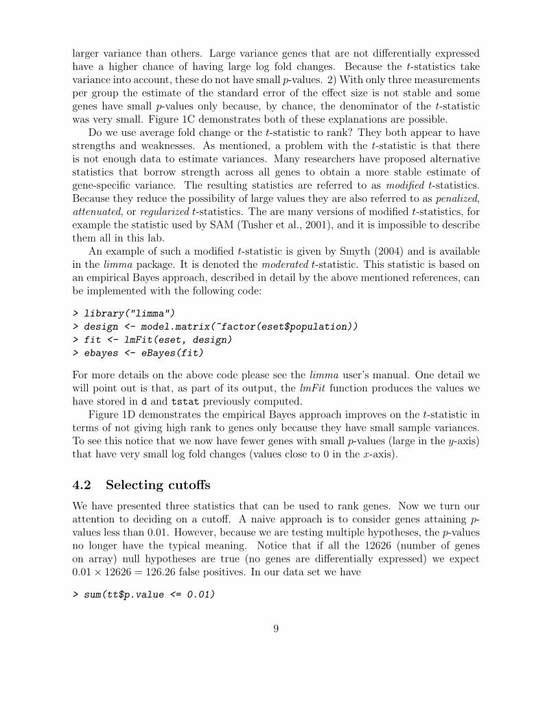
larger variance than others. Large variance genes that are not differentially expressedhave a higher chance of having large log fold changes. Because the t-statistics takevariance into account, these do not have small p-values. 2) With only three measurementsper group the estimate of the standard error of the effect size is not stable and somegenes have small p-values only because, by chance, the denominator of the t-statisticwas very small. Figure 1C demonstrates both of these explanations are possible.

Do we use average fold change or the t-statistic to rank? They both appear to havestrengths and weaknesses. As mentioned, a problem with the t-statistic is that thereis not enough data to estimate variances. Many researchers have proposed alternativestatistics that borrow strength across all genes to obtain a more stable estimate ofgene-specific variance. The resulting statistics are referred to as modified t-statistics.Because they reduce the possibility of large values they are also referred to as penalized,attenuated, or regularized t-statistics. The are many versions of modified t-statistics, forexample the statistic used by SAM (Tusher et al., 2001), and it is impossible to describethem all in this lab.

An example of such a modified t-statistic is given by Smyth (2004) and is availablein the limma package. It is denoted the moderated t-statistic. This statistic is based onan empirical Bayes approach, described in detail by the above mentioned references, canbe implemented with the following code:

> library("limma")

> design <- model.matrix(~factor(eset$population))

> fit <- lmFit(eset, design)

> ebayes <- eBayes(fit)

For more details on the above code please see the limma user’s manual. One detail wewill point out is that, as part of its output, the lmFit function produces the values wehave stored in d and tstat previously computed.

Figure 1D demonstrates the empirical Bayes approach improves on the t-statistic interms of not giving high rank to genes only because they have small sample variances.To see this notice that we now have fewer genes with small p-values (large in the y-axis)that have very small log fold changes (values close to 0 in the x-axis).

4.2 Selecting cutoffs

We have presented three statistics that can be used to rank genes. Now we turn ourattention to deciding on a cutoff. A naive approach is to consider genes attaining p-values less than 0.01. However, because we are testing multiple hypotheses, the p-valuesno longer have the typical meaning. Notice that if all the 12626 (number of geneson array) null hypotheses are true (no genes are differentially expressed) we expect0.01× 12626 = 126.26 false positives. In our data set we have

> sum(tt$p.value <= 0.01)

9

[1] 46

Various approaches have been suggested for dealing with the multiple hypothesisproblem. The suggested procedures usually provide adjusted p-values that can be usedto decide on appropriate cutoffs. However, different procedures result in different inter-pretations of the resulting lists. In Section 5, we demonstrate simple code that can beused, along with the results of the eBayes function described above, to construct lists ofgenes based on adjusted p-values.

An alternative ad hoc procedure is to use the MA and volcano plots to look for groupsof genes that appear to be departing from the majority. For example, in Figure 1C wecan restrict our attention to the small cluster of genes in the upper right corner havingsmall p-value and large fold changes.

4.3 Comparison

We deviate slightly from our analysis to demonstrate that the moderated t-statisticappears to perform better than average log fold change and the t-test.

Because we are using a spike-in experiment we can assess the three competing statis-tics. First we obtain the names of the genes that were spiked-in. This is available in theoriginal phenoData.

> data(spikein95)

> spikedin <- colnames(pData(spikein95))

> spikedIndex <- match(spikedin, geneNames(eset))

Because in this experiment replicate RNA, except for the spiked-in material, washybridized to all arrays, only the 16 spiked-in genes should be differentially expressed.This means that a perfect ranking procedure would assign ranks from 1 to 16 to the 16spiked-in genes. The following code shows that the moderated t-statistic is performingbetter than its three competitors.

> d.rank <- sort(rank(-abs(d))[spikedIndex])

> t.rank <- sort(rank(-abs(tt$statistic))[spikedIndex])

> mt.rank <- sort(rank(-abs(mtstat))[spikedIndex])

> ranks <- cbind(mt.rank, d.rank, t.rank)

> rownames(ranks) <- NULL

> ranks

mt.rank d.rank t.rank

[1,] 1 1 1

[2,] 2 2 3

[3,] 3 3 5

[4,] 6 4 8

10

[5,] 7 5 13

[6,] 8 6 17

[7,] 9 9 19

[8,] 10 11 27

[9,] 11 12 28

[10,] 12 14 29

[11,] 16 16 45

[12,] 25 53 70

[13,] 28 86 71

[14,] 48 226 93

[15,] 77 331 390

[16,] 465 689 900

The results above permit us to see how many true positives we would have in a list ofany size ranked by each of the three statistics. To do this, we simply count the number ofspiked-in genes with ranks smaller or equal to the size of the list. As an example noticethat in a list of the top 25 genes, we would obtain 12, 11, and 7 true positives for themoderated t-statistic. This demonstrates that the choice of ranking statistic can havean effect on your final results. Also notice that this is just one analysis, and one wouldexpect different results with a new data set. We encourage users to run this analysis onother data sets and assess the performance of different alternative procedures.

5 Annotation

Let us now consider a list of interesting genes and create a report. As an example wewill consider the top 10 genes as ranked by the moderated t-statistic. To do this we canuse the topTable function from the limma package in the following way:

> tab <- topTable(ebayes, coef = 2, adjust = "fdr", n = 10)

This function creates a table showing various interesting statistics. This line of codeshows us the first 5 entries:

> tab[1:5, ]

ID M A t P.Value B

780 1708_at -7.0610613 7.945276 -73.529269 9.868948e-13 8.646866

6253 36202_at 0.8525527 9.373033 9.975114 3.115897e-03 4.587736

6363 36311_at 0.8318298 8.564315 8.363252 1.269758e-02 3.567790

3285 33264_at 0.7118997 4.918953 7.434888 2.706595e-02 2.835849

2675 32660_at 0.6554022 8.680132 7.356180 2.706595e-02 2.768151

11

By specifying coef as 2 we define d as our parameter of interest. The argument n defineshow many top genes to include in the table. Finally, through adjust we are instructingtopTable to calculate the false discovery rate adjustment for the p-values obtained fromeBayes using the procedure described by Benjamini and Hochberg (1995). See the limmauser’s manual for more details.

In the remainder of this lab, we will use the Affymetrix identifiers to obtain biologicalmeta-data information about these 10 genes. We can obtain these using the ID columnof tab:

> genenames <- as.character(tab$ID)

5.1 Annotation package overview

First, we will digress slightly to explain the various metaData packages that are availablefrom Bioconductor. The metaData packages can be divided into three groups:

• General annotation (GO, KEGG)

• Species level annotation (xxxhomology, YEAST)

• Chip level annotation (hgu133plus2, rat4302, etc.)

Each of these metaData packages contain one or more environments which are similarto hash tables. A hash table provides a very quick way of looking up values using a key.We can use the functions get, and mget to extract data from a given environment. Asan example, we will use the hgu95av2 package. Note that this package contains severalenvironments, most of which use the Affymetrix probe IDs as keys.

> library("hgu95av2")

> hgu95av2()

Quality control information for hgu95av2

Date built: Created: Tue May 17 16:16:13 2005

Number of probes: 12625

Probe number missmatch: None

Probe missmatch: None

Mappings found for probe based rda files:

hgu95av2ACCNUM found 12625 of 12625

hgu95av2CHRLOC found 11718 of 12625

hgu95av2CHR found 12261 of 12625

hgu95av2ENZYME found 1804 of 12625

12

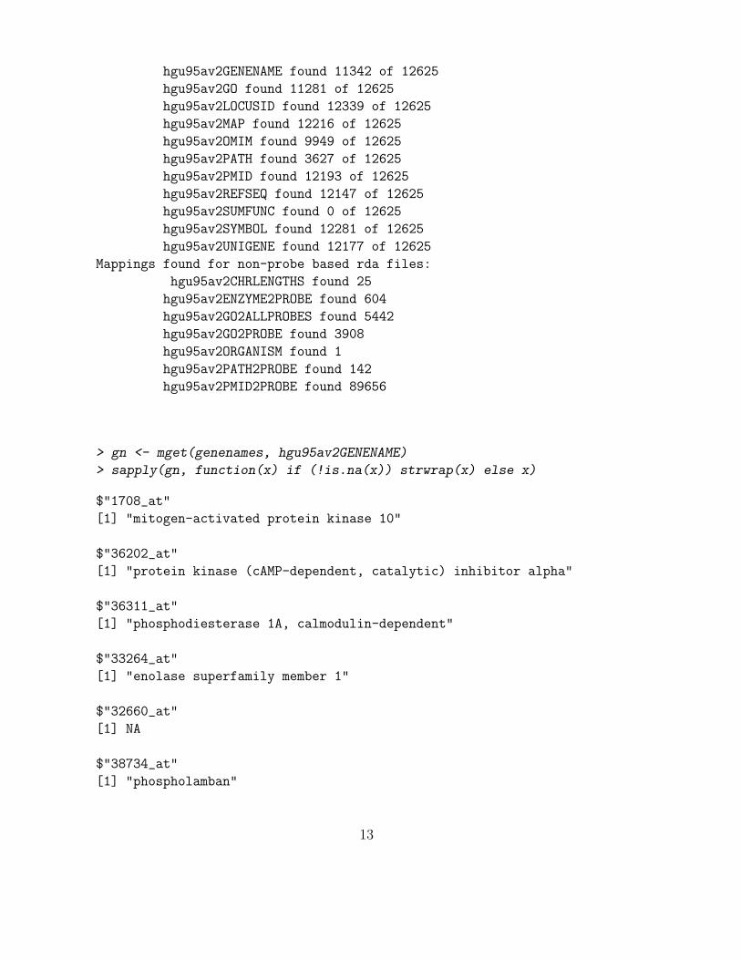
hgu95av2GENENAME found 11342 of 12625

hgu95av2GO found 11281 of 12625

hgu95av2LOCUSID found 12339 of 12625

hgu95av2MAP found 12216 of 12625

hgu95av2OMIM found 9949 of 12625

hgu95av2PATH found 3627 of 12625

hgu95av2PMID found 12193 of 12625

hgu95av2REFSEQ found 12147 of 12625

hgu95av2SUMFUNC found 0 of 12625

hgu95av2SYMBOL found 12281 of 12625

hgu95av2UNIGENE found 12177 of 12625

Mappings found for non-probe based rda files:

hgu95av2CHRLENGTHS found 25

hgu95av2ENZYME2PROBE found 604

hgu95av2GO2ALLPROBES found 5442

hgu95av2GO2PROBE found 3908

hgu95av2ORGANISM found 1

hgu95av2PATH2PROBE found 142

hgu95av2PMID2PROBE found 89656

> gn <- mget(genenames, hgu95av2GENENAME)

> sapply(gn, function(x) if (!is.na(x)) strwrap(x) else x)

$"1708_at"

[1] "mitogen-activated protein kinase 10"

$"36202_at"

[1] "protein kinase (cAMP-dependent, catalytic) inhibitor alpha"

$"36311_at"

[1] "phosphodiesterase 1A, calmodulin-dependent"

$"33264_at"

[1] "enolase superfamily member 1"

$"32660_at"

[1] NA

$"38734_at"

[1] "phospholamban"

13

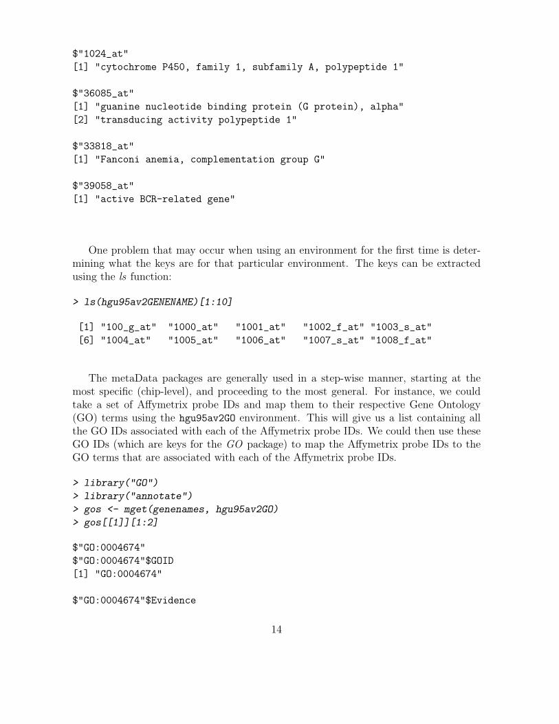
$"1024_at"

[1] "cytochrome P450, family 1, subfamily A, polypeptide 1"

$"36085_at"

[1] "guanine nucleotide binding protein (G protein), alpha"

[2] "transducing activity polypeptide 1"

$"33818_at"

[1] "Fanconi anemia, complementation group G"

$"39058_at"

[1] "active BCR-related gene"

One problem that may occur when using an environment for the first time is deter-mining what the keys are for that particular environment. The keys can be extractedusing the ls function:

> ls(hgu95av2GENENAME)[1:10]

[1] "100_g_at" "1000_at" "1001_at" "1002_f_at" "1003_s_at"

[6] "1004_at" "1005_at" "1006_at" "1007_s_at" "1008_f_at"

The metaData packages are generally used in a step-wise manner, starting at themost specific (chip-level), and proceeding to the most general. For instance, we couldtake a set of Affymetrix probe IDs and map them to their respective Gene Ontology(GO) terms using the hgu95av2GO environment. This will give us a list containing allthe GO IDs associated with each of the Affymetrix probe IDs. We could then use theseGO IDs (which are keys for the GO package) to map the Affymetrix probe IDs to theGO terms that are associated with each of the Affymetrix probe IDs.

> library("GO")

> library("annotate")

> gos <- mget(genenames, hgu95av2GO)

> gos[[1]][1:2]

$"GO:0004674"

$"GO:0004674"$GOID

[1] "GO:0004674"

$"GO:0004674"$Evidence

14

[1] "IEA"

$"GO:0004674"$Ontology

[1] "MF"

$"GO:0004705"

$"GO:0004705"$GOID

[1] "GO:0004705"

$"GO:0004705"$Evidence

[1] "ISS"

$"GO:0004705"$Ontology

[1] "MF"

> goids <- sapply(gos, names)

> goids[[1]]

[1] "GO:0004674" "GO:0004705" "GO:0004707" "GO:0004708" "GO:0005524"

[6] "GO:0006468" "GO:0007165" "GO:0007254" "GO:0016740"

> goterms <- sapply(goids, function(x) mget(as.character(x),

+ GOTERM))

> sapply(goterms[[1]], Term)

GO:0004674

"protein serine/threonine kinase activity"

GO:0004705

"JUN kinase activity"

GO:0004707

"MAP kinase activity"

GO:0004708

"MAP kinase kinase activity"

GO:0005524

"ATP binding"

GO:0006468

"protein amino acid phosphorylation"

GO:0007165

15

"signal transduction"

GO:0007254

"JNK cascade"

GO:0016740

"transferase activity"

Exercise 3We have shown how to extract GO terms, starting with a set of Affymetrix identifiers.The hgu95av2PATH environment maps Affymetrix IDs to the Kyoto Encyclopedia ofGenes and Geneomes (KEGG), which maintains pathway information for various organ-isms. As can be seen above, only about 25% of the Affymetrix IDs actually map to apathway – the remaining key values simply return an NA.

Extract the first five KEGG pathway IDs from hgu95av2PATH and using the KEGGpackage, map them to the respective pathway name. See the help page for hgu95av2PATHfor a hint.

This section showed how to extract data from environments ’by hand’. Althoughthis sort of thing can be tedious, it is sometimes necessary, so it is worth knowinghow it is done. However, the annotate and annaffy packages supply powerful tools forautomated extraction of annotation information that can be used in most situations. Inthe following sections, we present some simple examples.

5.2 PubMed abstracts

The annotate package contains many functions that can be used to query the PubMeddatabase and format the results. Here we show how some of these can be used to obtainabstracts with references to a list of genes and report findings in the form of a Web page.Specifically, to get the abstract information we can use the pm.getabst in the annotatepackage (which requires the XML package):

> library("XML")

> absts <- pm.getabst(genenames, "hgu95av2")

The return value absts is a list of the same length as the genenames argument. Each ofthe list’s components corresponds to a gene and is itself a list. Each component of thislist is an abstract for that gene. To see the fourth abstract for the first gene, we typethe following:

> absts[[1]][[4]]

An object of class ’pubMedAbst’:

Title: JNK1, JNK2 and JNK3 are p53 N-terminal serine 34

kinases.

PMID: 9393873

16

Authors: MC Hu, WR Qiu, YP Wang

Journal: Oncogene

Date: Nov 1997

Please be careful using the function pm.getabst because it queries PubMed directly.Too many queries of PubMed can get you banned.

To only see the titles for, say, the second probeset, we can type the following.

> titl <- sapply(absts[[2]], articleTitle)

> strwrap(titl, simplify = FALSE)

[[1]]

[1] "Isolation and characterization of cDNA clones for an"

[2] "inhibitor protein of cAMP-dependent protein kinase."

[[2]]

[1] "Inhibition of protein kinase-A by overexpression of the"

[2] "cloned human protein kinase inhibitor."

[[3]]

[1] "Structure of a peptide inhibitor bound to the catalytic"

[2] "subunit of cyclic adenosine monophosphate-dependent protein"

[3] "kinase."

[[4]]

[1] "Identification of an inhibitory region of the heat-stable"

[2] "protein inhibitor of the cAMP-dependent protein kinase."

[[5]]

[1] "Primary-structure requirements for inhibition by the"

[2] "heat-stable inhibitor of the cAMP-dependent protein kinase."

[[6]]

[1] "The expression and intracellular distribution of the"

[2] "heat-stable protein kinase inhibitor is cell cycle regulated."

[[7]]

[1] "Glutamic acid 203 of the cAMP-dependent protein kinase"

[2] "catalytic subunit participates in the inhibition by two"

[3] "isoforms of the protein kinase inhibitor."

[[8]]

[1] "Evidence for the importance of hydrophobic residues in the"

17

[2] "interactions between the cAMP-dependent protein kinase"

[3] "catalytic subunit and the protein kinase inhibitors."

[[9]]

[1] "Generation and initial analysis of more than 15,000"

[2] "full-length human and mouse cDNA sequences."

Here we used the strwrap function to format the text to fit the page width.Having these abstracts as R objects is useful because, for example, we can search for

words in the abstract automatically. The code below searches for the word “protein” inall the abstracts and returns a logical value:

> pro.res <- sapply(absts, function(x) pm.abstGrep("[Pp]rotein",

+ x))

> pro.res[[2]]

[1] TRUE TRUE TRUE TRUE TRUE TRUE TRUE TRUE FALSE

A convenient way to view the abstracts is to create a Web page:

> pmAbst2HTML(absts[[2]], filename = "pm.html")

The above code creates an HTML file with abstracts for the second probeset in gene-

names.

5.3 Generating reports

The object top gives us valuable information about the top 10 genes. However, it isconvenient to create a more informative table. We can easily add annotation to thistable and create an HTML document with hyperlinks to sites with more informationabout the genes. The following code obtains the Entrez Gene ID, UniGene ID, andsymbol for each of our selected genes.

> ll <- getLL(genenames, "hgu95av2")

> ug <- unlist(lookUp(genenames, "hgu95av2", "UNIGENE"))

> sym <- getSYMBOL(genenames, "hgu95av2")

With these values available, we can use the following code to create an HTML pageuseful for sharing results with collaborators.

> tab <- data.frame(sym, tab[, -1])

> htmlpage(list(ll, ug), filename = "report.html", title = "HTML report",

+ othernames = tab, table.head = c("Locus ID", "UniGene ID",

+ colnames(tab)), table.center = TRUE, repository = list("ll",

+ "ug"))

18

This HTML report contains links to both Entrez Gene and UniGene. However,htmlpage can only make links to a limited number of online databases, and is primarilyintended for microarrays that do not have chip-level annotation packages. For thosemicroarrays that do have annotation packages, we can use the annaffy package. Beloware a few lines of code that create a useful HTML report with links to various annotationsites.

> library("annaffy")

> atab <- aafTableAnn(genenames, "hgu95av2", aaf.handler())

> saveHTML(atab, file = "report2.html")

Exercise 4The annaffy package can be used to create HTML (and text) tables that contain notonly links to various online databases, but that contain additional information as well.It useful to append the expression values and statistics for the genes that are beingannotated, which gives you and your collaborators the ability to perform ’sanity checks’to ensure that no coding errors have been made in selecting a set of genes.

Reproduce the above HTML table, but include the t-statistic, p-value, and expressionvalues for each gene. Also limit the number of links to only include the Affymetrix ID,UniGene, Entrez Gene, and PubMed.

5.4 Statistics based on Annotation

Given a set of differentially regulated genes, it is fairly common to ask if certain pathwaysare being perturbed in some way. This is a difficult question to answer given the fact thatmost genes (75% of the genes on the HG-U95Av2 chip, for instance) are not mapped toany pathway. As a surrogate, we can look for GO terms that appear to be ’concentrated’in a set of differentially expressed genes using the GOHyperG function in the GOstatspackage. If we find that the number of genes with a certain GO term are overrepresentedin the set of differentially expressed genes, then this may imply that a particular pathwayor function is being affected.

> library("GOstats")

> index <- sample(1:12000, 100)

> gn <- ls(hgu95av2GENENAME)[index]

> lls <- unique(getLL(gn, "hgu95av2"))

> hyp <- GOHyperG(lls, "hgu95av2", what = "MF")

> index2 <- hyp$pvalues < 0.05

> wh <- mget(names(hyp$pvalues)[index2], GOTERM)

> terms <- sapply(wh, Term)

> strwrap(terms[1:10], simplify = FALSE)

19

[[1]]

[1] "GTP cyclohydrolase activity"

[[2]]

[1] "GTP cyclohydrolase I activity"

[[3]]

[1] "4-alpha-hydroxytetrahydrobiopterin dehydratase activity"

[[4]]

[1] "glycogen synthase kinase 3 activity"

[[5]]

[1] "poly(ADP-ribose) glycohydrolase activity"

[[6]]

[1] "luteinizing hormone-releasing factor activity"

[[7]]

[1] "hydrolase activity, hydrolyzing O-glycosyl compounds"

[[8]]

[1] "L-malate dehydrogenase activity"

[[9]]

[1] "arachidonate 12-lipoxygenase activity"

[[10]]

[1] "succinate dehydrogenase (ubiquinone) activity"

> hyp$pvalues[index2][1:10]

GO:0003933 GO:0003934 GO:0008124 GO:0004696 GO:0004649 GO:0005183

0.01086957 0.01086957 0.01086957 0.01086957 0.01086957 0.01086957

GO:0004553 GO:0030060 GO:0004052 GO:0008177

0.01506284 0.02162243 0.02162243 0.02162243

Exercise 5The above code is an example of something that could easily become quite tedious if ithad to be repeated more than one or two times. It is often worth the time and effort

20

to write a small ’wrapper’ function that will perform all the required steps to take e.g.,a vector of Affymetrix probe IDs and output a data.frame containing the GO ID, GOterm, p-value, the number of genes with that GO term in the set of significant genes,and the number on the chip. The last two bits of information are good to know becauseit is easy to get a very small p-value when there are few genes with a given GO termon the chip (e.g., if there are three genes with a GO term XXX, and one is in the listof significant genes, you will get a small p-value, but it is probably not an interestingresult).

If we have time (and you feel up to it), write a wrapper function to do this, outputtingthe results as a data.frame.

6 Conclusion

We have demonstrated how one can use Bioconductor tools to go from the raw data inCEL files to annotated reports of a select group of interesting genes. We presented onlyone way of doing this. There are many alternatives also available via Bioconductor. Wehope that this lab serves as an example of a useful analysis and also of the flexibility ofBioconductor.

References

Affymetrix. GeneChip Expression Analysis Technical Manual. Affymetrix, Santa Clara,CA, rev 4.0 edition, 2003.

Y. Benjamini and Y. Hochberg. Controlling the false discovery rate: a practical andpowerful approach to multiple testing. Journal of the Royal Statistical Society, SeriesB, 57:289–300, 1995.

Rafael A. Irizarry, Bridget Hobbs, Francois Collin, et al. Exploration, normalization,and summaries of high density oligonucleotide array probe level data. Biostatistics, 4:249–64, 2003.

Cheng Li and Wing Hung Wong. Model-based analysis of oligonucleotide arrays: Ex-pression index computation and outlier detection. Proc. Natl. Acad. Sci., 98:31–36,2001.

Mary E. Ross, Xiaodong Zhou, Guangchun Song, et al. Gene expression profiling ofpediatric acute myelogenous leukemia. Blood, 102:2951–2959, 2004.

G.K. Smyth. Linear models and empirical Bayes methods for assessing differential ex-pression in microarray experiments. Statistical Applications in Genetics and MolecularBiology, 3:Article 3, 2004.

21

V.G. Tusher, R. Tibshirani, and G. Chu. Significance analysis of microarrays applied tothe ionizing radiation response. Proc. Natl. Acad. Sci., 98:5116–5121, 2001.

Zhijin Wu, RA Irizarry, R Gentleman, F Martinez Murillo, and F Spencer. A modelbased background adjustement for oligonucleotide expression arrays. Journal of theAmerican Statistical Association, to appear, 2005.

22