BIOCHLORBIOCHLORBIOCHLORBIOCHLORBIOCHLORNatural Attenuation DecisionNatural Attenuation DecisionNatural Attenuation DecisionNatural Attenuation DecisionNatural Attenuation DecisionSupport SystemSupport SystemSupport SystemSupport SystemSupport System

User’s ManualUser’s ManualUser’s ManualUser’s ManualUser’s ManualVersion 1.0Version 1.0Version 1.0Version 1.0Version 1.0

United StatesEnvironmental ProtectionAgency

Office of Research andDevelopmentWashington DC 20460

EPA/600/R-00/008January 2000

SURFACE

TOP OFWATER-BEARING

UNIT

BOTTOM OFWATER-BEARING

UNIT

BIOCHLORBIOCHLORBIOCHLORBIOCHLORBIOCHLOR

Natural Attenuation Decision Support SystemNatural Attenuation Decision Support SystemNatural Attenuation Decision Support SystemNatural Attenuation Decision Support SystemNatural Attenuation Decision Support System

User’s ManualUser’s ManualUser’s ManualUser’s ManualUser’s ManualVersion 1.0Version 1.0Version 1.0Version 1.0Version 1.0

by

Carol E. Aziz and Charles J. NewellGroundwater Services, Inc.

Houston, Texas

James R. Gonzales and Patrick HaasTechnology Transfer Division

Air Force Center for Environmental ExcellenceBrooks AFB, San Antonio, Texas

T. Prabhakar Clement and Yunwei SunBattelle Pacific Northwest National Laboratory

Richland, Washington

Project Officer

David G. JewettSubsurface Protection and Remediation DivisionNational Risk Management Research Laboratory

Ada, Oklahoma 74820

NATIONAL RISK MANAGEMENT RESEARCH LABORATORYOFFICE OF RESEARCH AND DEVELOPMENT

U.S. ENVIRONMENTAL PROTECTION AGENCYCINCINNATI, OHIO 45268

EPA/600/R-00/008

January 2000

NOTICE

The information in this document was developed through a collaboration between the U.S. EPA (SubsurfaceProtection and Remediation Division, National Risk Management Research Laboratory, Robert S. KerrEnvironmental Research Center, Ada, Oklahoma [RSKERC]) and the U.S. Air Force (U.S. Air Force Centerfor Environmental Excellence, Brooks Air Force Base, Texas). EPA staff contributed conceptual guidancein the development of the BIOCHLOR mathematical model. To illustrate the appropriate application ofBIOCHLOR, EPA contributed field data generated by EPA staff supported by ManTech EnvironmentalResearch Services Corp, the in-house analytical support contractor at the RSKERC. The computer code forBIOCHLOR was developed by Groundwater Services, Inc. through a contract with the U.S. Air Force.Groundwater Services, Inc. also provided field data to illustrate the application of the model.

All data generated by EPA staff or by ManTech Environmental Research Services Corp were collectedfollowing procedures described in the field sampling Quality Assurance Plan for an in-house researchproject on natural attenuation, and the analytical Quality Assurance Plan for ManTech EnvironmentalResearch Services Corp. The development of BIOCHLOR and its User’s Manual were not funded by theU.S. EPA and as such are not subject to the Agency’s QA requirements.

An extensive investment in site characterization and mathematical modeling is often necessary to establishthe contribution of natural attenuation at a particular site. BIOCHLOR is offered as a screening tool todetermine whether it is appropriate to invest in a full-scale evaluation of natural attenuation at a particularsite. Because BIOCHLOR incorporates a number of simplifying assumptions, it is not a substitute for thedetailed mathematical models that are necessary for making final regulatory decisions at complex sites.

BIOCHLOR and its User’s Manual have undergone external and internal peer review conducted by the U.S.EPA and the U.S. Air Force. However, BIOCHLOR is made available on an as-is basis without guaranteeor warranty of any kind, express or implied. Neither the United States Government (U.S. EPA or U.S. AirForce), Ground Water Services, Inc., any of the authors nor reviewers accept any liability resulting from theuse of BIOCHLOR or its documentation. Implementation of BIOCHLOR and interpretation of the predictionsof the model are the sole responsibility of the user.

ii

FOREWORD

The U.S. Environmental Protection Agency is charged by Congress with protecting the Nation’s land, air,and water resources. Under a mandate of national environmental laws, the Agency strives to formulate andimplement actions leading to a compatible balance between human activities and the ability of naturalsystems to support and nurture life. To meet these mandates, EPA’s research program is providing data andtechnical support for solving environmental problems today and building a science knowledge basenecessary to manage our ecological resources wisely, understand how pollutants affect our health, andprevent or reduce environmental risks in the future.

The National Risk Management Research Laboratory is the Agency’s center for investigation of technologi-cal and management approaches for reducing risks from threats to human health and the environment. Thefocus of the Laboratory’s research program is on methods for the prevention and control of pollution to air,land, water, and subsurface resources; protection of water quality in public water systems; remediation ofcontaminated sites and ground water; and prevention and control of indoor air pollution. The goal of thisresearch effort is to catalyze development and implementation of innovative, cost-effective environmentaltechnologies; develop scientific and engineering information needed by EPA to support regulatory and policydecisions; and provide technical support and information transfer to ensure effective implementation ofenvironmental regulations and strategies.

This screening tool will allow ground water remediation managers to identify sites where natural attenuationis most likely to be protective of human health and the environment. It will also allow regulators to carry outan independent assessment of treatability studies and remedial investigations that propose the use ofnatural attenuation.

Clinton W. Hall, DirectorSubsurface Protection and Remediation DivisionNational Risk Management Research Laboratory

iii

iv

Acknowledgments

BIOCHLOR was developed by Drs. Carol Aziz and Charles Newell (Groundwater Services, Inc., Houston,TX). Customization and testing of the BIOCHLOR solution engine was performed by Drs. PrabhakarClement and Yunwei Sun (Battelle Pacific Northwest National Laboratory, Richland, WA).

The authors would like to acknowledge the U.S. Air Force Center for Environmental Excellence (AFCEE) forsupporting the development of BIOCHLOR. We would like to specifically acknowledge Marty Faile and JimGonzales.

We also wish to acknowledge Ann Smith (Radian International, Austin, TX) for contributing to thedevelopment of BIOCHLOR. Special thanks also to Phil deBlanc, Leigh Ita, Ric Bowers, Julia Aziz, TariqKhan, and Martha Williams.

The BIOCHLOR software and manual was reviewed by a distinguished review team. We wish toacknowledge members of the team for their comments and suggestions:

Dr. Harry Beller, Lawrence Livermore National Laboratory, Livermore, CA

Ned Black, U.S. EPA, Region 9, San Francisco, CA

Joan Elliott, U.S. EPA National Risk Management Research Laboratory, Ada, OK

Dr. Rolf Halden, Lawrence Livermore National Laboratory, Livermore, CA

Enamul Hoque, ManTech Environmental Research Services Corp., Ada, OK

Dr. David Jewett, U.S. EPA National Risk Management Research Laboratory, Ada, OK

Dr. Ann Azadpour-Keeley, U.S. EPA National Risk Management Research Laboratory, Ada, OK

Dr. Roger Lee, U.S. Geological Survey, Dallas, TX

Herb Levine, U.S. EPA, Region 9, San Francisco, CA

Dr. Elise Striz, ManTech Environmental Research Services Corp., Ada, OK

Luanne Vanderpool, U.S. EPA Region 5, Chicago, IL

v

Contents

Introduction ...................................................................................................................................1Intended Uses for BIOCHLOR ...................................................................................................... 1Fundamentals of Natural Attenuation............................................................................................2

Overview of Natural Attenuation...........................................................................................2Natural Attenuation Lines of Evidence and the Role of BIOCHLOR ....................................4

BIOCHLOR Concepts ...................................................................................................................6BIOCHLOR Model Types...................................................................................................... 6

BIOCHLOR Data Entry .................................................................................................................61. Hydrogeologic Data ..........................................................................................................72. Dispersivity .......................................................................................................................93. Adsorption Data..............................................................................................................104. Biotransformation Data ...................................................................................................125. General Data ..................................................................................................................146. Source Data ...................................................................................................................167. Field Data for Comparison..............................................................................................18

Analyzing BIOCHLOR Output .....................................................................................................19Centerline Output ...............................................................................................................19Array Output .......................................................................................................................19

Calculating the Mass Balance (Order-of-Magnitude Accuracy) ......................................19Quick Start ..................................................................................................................................21

Minimum System Requirements ........................................................................................21Installation and Start-Up ....................................................................................................21

BIOCHLOR TROUBLESHOOTING TIPS....................................................................................21Spreadsheet-Related Problems .........................................................................................21Common Error Messages ..................................................................................................21

References ..................................................................................................................................23Appendix A.1 Domenico Single Species Analytical Model ........................................................25Appendix A.2 ...............................................................................................................................27

Kinetics of Sequential First Order Decay ...........................................................................27Chlorinated Ethenes ...........................................................................................................27Chlorinated Ethanes ...........................................................................................................28Other Chlorinated Compounds ..........................................................................................281-Zone vs. 2 -Zone Biotransformation ...............................................................................28How BIOCHLOR Models 2-Zone Biotransformation ..........................................................30

Appendix A.3 ..............................................................................................................................31BIOCHLOR Solution ..........................................................................................................31Governing Equations ..........................................................................................................31Analytical Solution Strategy................................................................................................31Computational Procedure ..................................................................................................33

Appendix A.4 Dispersivity Estimates .........................................................................................36Appendix A.5 Pump and Treat Comparison ...............................................................................38Appendix A.6 ...............................................................................................................................39

BIOCHLOR Example ......................................................................................................40BIOCHLOR Modeling Summary, .....................................................................................42Cape Canaveral Air Station, Florida ................................................................................42Entering Input ..................................................................................................................42

vi

Viewing Output ................................................................................................................42Sensitivity Analysis Examples .........................................................................................46

vii

Figures

Figure 1. Reductive dechlorination pathways for common chlorinatedaliphatic hydrocarbons (from Vogel and McCarty, 1987). ........................................3

Figure 2. Reductive transformation of chlorinated ethenes. ....................................................3Figure 3. Initial screening process flow chart. ......................................................................... 5Figure A.1. Mixed type I/Type III plume conditions. ...................................................................29Figure A.2. Comparison of solution techniques for BIOCHLOR 1-zone and 2-zone

biotransformation models. ......................................................................................30Figure A.3. Longitudinal dispersivity vs. scale data reported by Gelhar et al. (1992). ..............37Figure A.4. Ratio of transverse dispersivity and vertical dispersivity to longitudinal

dispersivity data vs. scale reported by Gelhar et al. (1992). ...................................38Figure A.5. BIOCHLOR source zone assumption (TCE as example). ......................................41Figure A.6. BIOCHLOR input screen. Cape Canaveral Air Force Base, Florida. ......................43Figure A.7. Centerline output. Cape Canaveral Air Force Base, Florida. .................................44Figure A.8. Individual centerline output for TCE, Cape Canaveral Air Station, Florida. ............44Figure A.9. Array concentration output for TCE. Cape Canaveral Air Station, Florida. ............45

TablesTable A.1. 2-Zone Biotransformation Scenarios .........................................................................28Table A.2. Modeling Scenario 3 for Chlorinated Ethenes ...........................................................29Table A.3. Modeling Scenario 3 for Chlorinated Ethanes ...........................................................29Table A.4. Sensitivity Analysis Results - Rate Coefficients ........................................................46Table A.5. Sensitivity Analysis Results - Retardation Factor ......................................................46

1

Introduction

BIOCHLOR is an easy-to-use screening model that simulates remediation by natural attenuation (RNA) of dissolvedsolvents at chlorinated solvent release sites. The software, programmed in the Microsoft Excel spreadsheetenvironment and based on the Domenico analytical solute transport model, has the ability to simulate 1-D advection, 3-Ddispersion, linear adsorption, and biotransformation via reductive dechlorination (the dominant biotransformationprocess at most chlorinated solvent sites). Reductive dechlorination is assumed to occur under anaerobic conditionsand dissolved solvent degradation is assumed to follow a sequential first-order decay process. BIOCHLOR includesthree different model types:

1. Solute transport without decay,2. Solute transport with biotransformation modeled as a sequential first-order decay process,3. Solute transport with biotransformation modeled as a sequential first-order decay process with two different

reaction zones (i.e., each zone has a different set of rate coefficient values).BIOCHLOR was developed for the Air Force Center for Environmental Excellence (AFCEE) Technology TransferDivision at Brooks Air Force Base by Groundwater Services, Inc., Houston, Texas. The mathematical technique to solvethe coupled reactive transport equations was developed by researchers at the Battelle Pacific Northwest NationalLaboratory.

Intended Uses for BIOCHLORBIOCHLOR attempts to answer the following fundamental question regarding RNA:

• How far will a dissolved chlorinated solvent plume extend if no engineered controls or source areareduction measures are implemented?

BIOCHLOR uses an analytical solute transport model with sequential first-order decay for simulating in-situbiotransformation (Sun et al., 1999a; Sun and Clement, 1999). The model will predict the maximum extentof dissolved-phase plume migration, which may then be compared to the distance to potential points ofexposure (e.g., drinking water wells, ground-water discharge areas, or property boundaries). Analyticalground-water transport models have seen wide application for this purpose (e.g., ASTM, 1995) andexperience has shown such models can produce reliable results when site conditions in the plume area arerelatively uniform.

BIOCHLOR is intended to be used in two ways:

1. As a screening-level model to determine if RNA is feasible at a chlorinated solvent site.BIOCHLOR is intended to be used as a screening-level model to determine if natural attenuation isoccurring at sufficient rates at a site to warrant a full natural attenuation study. Ideally, site-specificbiotransformation rate constants should be employed, but literature values can be used if measured rateconstants are unavailable. Other useful attributes of BIOCHLOR include the facilitation of site characteriza-tion data organization and the ability to carry out many simulations in short periods of time. For fuelhydrocarbon release sites, the BIOSCREEN model (Newell et al., 1996) is more appropriate.

2. As an RNA ground-water model to address selected chlorinated solvent problemsThe Technical Protocol for Evaluating Natural Attenuation of Chlorinated Solvents in Ground Water (U.S.EPA, 1998) describes how ground-water models, in conjunction with other types of analysis, can be usedto evaluate the effectiveness of natural attenuation. BIOCHLOR is an appropriate model at sites wheresimplifying assumptions (e.g., uniform ground-water flow, a vertical plane source, first-order decay) can be

2

made so that the resulting simulations provide useful information for the problem being addressed. At othersites, where these assumptions do not hold, a more sophisticated numerical model such as RT3D(Clement, 1997) would be appropriate. As with any modeling study, the authors recommend that propercare be used to select the model that is best suited to 1) the source, hydrogeology, and biotransformationprocesses present at the site and, 2) the type of problem being addressed (e.g., screening of alternatives,providing supporting evidence of natural attenuation, developing detailed design information).

BIOCHLOR has the following limitations:

1. As an analytical model, BIOCHLOR assumes simple ground-water flow conditions.

The model should not be applied where pumping systems create a complicated flow field. In addition, themodel should not be applied where vertical flow gradients affect contaminant transport. (Note that a verticaldistribution of chlorinated solvents throughout the saturated zone does not preclude the use of BIOCHLOR,as this phenomenon is related to the initial vertical migration of dense non-aqueous phase liquids in sourceareas.)

2. As a screening tool, BIOCHLOR assumes uniform hydrogeologic and environmental conditions over theentire model area.

Being an analytical model, BIOCHLOR assumes constant source, hydrogeological, and biological propertyvalues for the entire model area and, therefore, simplifies actual site conditions. For this reason, the modelshould not be applied where extremely detailed, accurate results that closely match site conditions arerequired. More comprehensive numerical models should be applied in such cases.

3. BIOCHLOR is primarily designed for simulating the sequential reductive dechlorination of chlorinatedethanes and ethenes.

The sequential biotransformation feature in BIOCHLOR should not be used for compounds that do notdegrade via sequential first-order kinetics. While the interface is designed for simulating the biotransforma-tion of chlorinated ethenes (i.e., PCE, TCE, DCE, and vinyl chloride (VC)) and chlorinated ethanes (i.e.,TCA, DCA, and chloroethane (CA)), the model can be adapted for other sequential decay reactions byexperienced users (see Appendix A.2).

Fundamentals of Natural AttenuationOverview of Natural Attenuation“Natural Attenuation” refers to naturally-occurring processes in soil and ground-water environments that act withouthuman intervention to reduce the mass, toxicity, mobility, volume, or concentration of contaminants in those media.These in-situ processes include biotransformation, dispersion, dilution, adsorption, volatilization, and chemical orbiological stabilization or destruction of contaminants (U.S.EPA, 1998).

Biotransformation can often be a dominant process in the natural attenuation of chlorinated solvents. At chlorinatedsolvent contaminated sites, most of the solvent degradation occurs by reductive dechlorination (U.S.EPA, 1998).Reductive dechlorination is a microbially-mediated reaction whereby a chlorine atom on the chlorinated solvent isreplaced by a hydrogen atom (Vogel and McCarty, 1987). In many bioremediation processes, an organic contaminant(such as benzene) acts as an electron donor and another substance (such as oxygen, nitrate, etc.) acts as the electronacceptor. However, during reductive dechlorination, hydrogen acts as the electron donor and halogenated compounds,such as chlorinated solvents, act as electron acceptors and thus become reduced, as shown in the following halfreaction:

R-Cl + H+ + 2e- ———> R-H + Cl-

Figure 1 shows the reductive transformation pathways for the common chlorinated aliphatics. More details on thebiotransformation of chlorinated solvents can be found in Appendix A.2.

Reductive dechlorination can be modeled as a sequential first-order decay process. This means that a parent compoundundergoes first-order decay to produce a daughter product and that product undergoes first-order decay and so on.Generally, the more highly chlorinated the compound, the more rapidly it is reduced by reductive dechlorination (Vogeland McCarty, 1985; Vogel and McCarty, 1987). Therefore, it is possible for daughter products to increase inconcentration before they decrease as shown in Figure 2. BIOCHLOR accounts for sequential first-order decay of thisnature, and this sets it apart from BIOSCREEN (Newell et al., 1996), which models the biodegradation of fuelhydrocarbons via first-order decay or electron acceptor-limited (instantaneous reaction) processes.

3

For biological reductive dechlorination to occur, the following conditions must exist:

1. The subsurface environment must be anaerobic and have a low oxidation-reduction potential (ORP).

2. Chlorinated solvents that are amenable to reductive dechlorination must be present.

3. A population of dechlorinating bacteria must be present.

4. An adequate supply of fermentation substrates to produce dissolved hydrogen must be present.

The environmental chemistry and the ORP of a site play an important role in determining whether reductivedechlorination will occur. Based on thermodynamic considerations, reductive dechlorination will occur only after bothoxygen and nitrate have been depleted from the aquifer, because oxygen and nitrate are more energetically favorableelectron acceptors than chlorinated solvents when hydrogen is the electron donor (U.S. EPA, 1998).

The role of hydrogen as an electron donor during reductive dechlorination is now widely recognized as a key factorgoverning the dechlorination of chlorinated compounds (Gossett and Zinder, 1996; Holliger et al., 1993; Maymo-Gatell etal., 1997; Hughes et al., 1997; Carr and Hughes, 1998). The hydrogen is produced in the terrestrial subsurface by thefermentation of a wide variety of organic compounds including anthropogenic compounds such as petroleum hydrocar-bons and natural organic matter. Hydrogen is then used by the dechlorinating bacteria as an electron donor.

Although BIOCHLOR primarily models the degradation of chlorinated solvents via reductive dechlorination, which occursunder highly reduced anaerobic conditions, some of the chlorinated solvents may degrade under aerobic conditions.TCE, c-DCE and VC degrade cometabolically (McCarty and Semprini, 1994) and VC (Hartmans et al., 1985; Hartmansand de Bont, 1992) and possibly c-DCE (Bradley and Chapelle, 1998) can be directly oxidized to carbon dioxide underaerobic conditions. PCE has not been found to degrade aerobically (McCarty and Semprini, 1994).

Figure 2. Reductive transformation of chlorinated ethenes.

1,1,1-TCA 1,1-DCA Chloroethane

Cis-1,2-DCE

Trans-1,2-DCE

1,1-DCE

Vinyl ChloridePCE TCE

Ethane

CH3CH3

Major pathway

Minor pathway

Ethene

CH2CH2

TCADCA

= Trichloroethane= Dichlorethane

PCETCEDCE

= Perchloroethene= Trichloroethene= Dichloroethene

Figure 1. Reductive dechlorination pathways for common chlorinated aliphatic hydrocarbons (after Vogel and McCarty,1985; Vogel andMcCarty,1987).

4

Natural Attenuation Lines of Evidence and the Role of BIOCHLORTo support remediation by natural attenuation, it must be scientifically demonstrated that attenuation of the sitecontaminants is occurring at rates sufficient to be protective of human health and the environment. According to the“Technical Protocol For Evaluating Natural Attenuation of Chlorinated Solvents in Ground Water” (U.S. EPA, 1998), threelines of evidence can be used to support natural attenuation of chlorinated solvents including :

1. Observed reductions in contaminant concentrations along the flow path downgradient from the source ofcontamination.

2. Documented loss of contaminant mass at the field scale using:

a) Chemical and geochemical analytical data including decreasing parent compound concentration,increasing daughter compound concentrations, depletion of electron acceptors and donors, andincreasing metabolic byproduct concentrations; and/or

b) A rigorous estimate of residence time along the flow path to document contaminant mass reduction andto calculate biological decay rates at the field scale.

3. Laboratory microcosm or field data that support the occurrence of biotransformation and give rates ofbiotransformation.

At a minimum, the investigator must obtain the first two lines of evidence or the first and third lines of evidence. Thesecond or third line of evidence is crucial because it provides biotransformation rate constants. These rate constants canbe used in conjunction with other fate and transport parameters to predict contaminant concentration and to assess riskat a downgradient point of exposure (U.S. EPA, 1998).

Compared to fuel hydrocarbon plumes, use of natural attenuation as a stand-alone remedy for chlorinated solventplumes is appropriate for a much lower percentage of plumes, because of their longer plume lengths. Therefore, it isparticularly important to make an accurate assessment of the potential for natural attenuation prior to investing in adetailed natural attenuation study. To assist in this endeavor, the natural attenuation screening process is outlined inFigure 3. The shaded steps indicate the stages where BIOCHLOR plays a role in the screening process.

The first shaded stage (i.e., “Is Biodegradation Occurring?”) is the stage where the natural attenuation scoring systemcomes into play. The scoring system requires the concentrations of electron acceptors, parent and daughter chlorinatedsolvents, methane, TOC, and chloride and ORP, temperature, and pH measurements (U.S. EPA, 1998). These fielddata are evaluated and scored for evidence of biotransformation. BIOCHLOR incorporates this scoring system, whichcan be accessed from the input page.

If there is evidence of biotransformation, BIOCHLOR may be used subsequently to compare the rate of chlorinatedsolvent transport without biotransformation to the rate of attenuation with biotransformation. Being a transient model, thesimulation time can be varied to determine the future extent of contamination. Field-derived biological rate coefficientsshould be used if possible, but literature values may be used in the absence of site-specific rate constants or the modelmay be calibrated to field data.

The primary purpose of comparing the transport rate to the attenuation rate is to determine if the residence time along theflow path is adequate to protect human health and the environment (i.e., to estimate if the contaminant degrades to anacceptable concentration before receptors are exposed). In the case of rate coefficients or any other parameter that isnot known accurately or that varies over the extent of the plume, sensitivity analyses should be conducted. If modelingshows that the receptors will not be impacted by contaminants at concentrations above regulatory criteria, then thescreening criteria are met, and the investigator can proceed with a full natural attenuation evaluation. Details of a fullnatural attenuation evaluation can be found in “Technical Protocol For Evaluating Natural Attenuation of ChlorinatedSolvents in Ground Water” (U.S. EPA, 1998).

5

Figure 3. Initial screening process flow chart.

Analyze Available Site Data AlongCore of Plume to Determine ifBiodegradation is Occurring.

IsBiodegradation

Occurring?

YES

Collect More Screening Data.

Locate Source(s) and PotentiaPoints of Exposure. EstimateExtent of NAPL, Residual andFree-Phases.

AreSufficient Data

Available ?Engineered RemediationRequired. Implement OtherProtocols.

YESNO or

INSUFFICIENTDATA

Determine Groundwater Flowand Solute Transport ParametersAlong Core of Plume UsingSite-Specific Data; Porosity andDispersivity may be Estimated

Estimate Biodegradation RateConstant

Compare the Rate of Transportto the Rate of Attenuation usingAnalytical Solute TransportModel (BIOCHLOR).

AreScreening Criteria

Met ?

Does itAppear that Natural

Attenuation Alone willMeet Regulatory

Criteria ?

YES

YES

NO

NO

Perform Site Characterization toEvaluate Natural Attenuation.

Evaluate use of SelectedAdditional Remedial Optionsalong with Natural Attenuation

PROCEED TO FULLNATURAL ATTENUATION STUDY

PROCEED TO FULLNATURAL ATTENUATION STUDY

NO

6

BIOCHLOR ConceptsThe BIOCHLOR Natural Attenuation software is based on a sequential, first-order, coupled reactive transport model.The transport problem is analytically solved using the Domenico model (1987) by uncoupling the transport equationsusing a novel analytical strategy (Sun et al., 1999a, 1999b; Sun and Clement, 1999) as discussed in Appendix A.3. Theoriginal Domenico model assumes a fully-penetrating vertical plane source oriented perpendicular to ground-water flowto simulate the release of organics to moving ground water and accounts for the effects of one-dimensional advectivetransport, three-dimensional dispersion, linear adsorption, and first-order decay. In BIOCHLOR, the Domenico solutionhas been adapted to provide three different model types representing i) transport with no decay, ii) transport withsequential first-order decay in one zone, and iii) transport with sequential first-order decay in two zones (see ModelTypes). Guidelines for selecting key input parameters for the model are outlined in BIOCHLOR Input Parameters. Forhelp on Output, see BIOCHLOR Output.

BIOCHLOR Model TypesThe software allows the user to view results from three different types of ground-water transport models:

1. Solute transport with no decay. This model is appropriate for predicting the movement of conservative(non-degrading) solutes. The only attenuation mechanisms are dispersion in the longitudinal, transverse,and vertical directions (if present), and adsorption of contaminants to the soil matrix (if present).

2. Solute transport with sequential first-order decay in one zone. With this model, the reactive transportof both parent and daughter chlorinated solvents can be modeled. This model accounts for dispersion,adsorption, advection, and sequential biotransformation. The reductive dechlorination of the parent solventto daughter product is assumed to be a first-order process. That is, the solute degradation rate is assumedto be proportional to the solute concentration. However, the daughter products are also produced by thefirst-order degradation of the preceding parent compound. Therefore, the daughter product can simultaneouslyundergo both production and degradation. "One zone" means that one set of rate constants is used withinthe model area. The model assumes that biotransformation starts immediately downgradient of the sourceand that no biotransformation of dissolved constituents in the source area occurs.

The sequential first-order decay model does not directly account for site-specific information such as theconcentration of the electron donor (i.e., hydrogen) or the number of dechlorinating bacteria; this is implicitlyaccounted for in the first-order decay rate coefficient supplied by the user. Ideally, rate coefficientsmeasured in the field or derived from model calibration to site data should be used. Literature values mayalso be employed, but the user must be aware that the literature value may have been measured underdifferent environmental conditions than those present for the plume being modeled.

3. Solute transport with sequential first-order decay in two zones. This model employs the samesequential first-order decay kinetics as the preceding model but allows the user to use two different sets ofrate constants within the model area. This may be appropriate for plumes that undergo rapid biotransformationclose to the source where there is an excess of fermentable substrates but negligible biotransformationfurther downgradient where fermentable substrates have been depleted or for plumes that go fromanaerobic conditions to aerobic conditions. Aerobic conditions can be considered only in the second zoneand should be modeled only by experienced users as discussed in Appendix A.2.

Note: This two-zone model should be employed only when the plume is at steady-state throughoutthe first zone. The plume is at steady-state if plume concentrations (field measurements or modelpredictions) are not changing with time. This condition is required to ensure the constant concentrationboundary condition at the boundary between zone 1 and zone 2. Refer to Appendix A.2 for a more detaileddiscussion.

BIOCHLOR Data EntryThree important considerations regarding data input are:

1. To see the example data set in the input screen of the software, click on the "Paste Example Data Set"button on the lower right portion of the input screen.

2. Because BIOCHLOR is based on the Excel spreadsheet, you must click outside of the cell where you justentered data or hit "return" before any of the buttons will work.

7

3. Parameters used in the model can be entered directly into the white cells or they can be calculated by themodel using data entered in the gray cells (e.g., seepage velocity can be entered directly or calculated usinghydraulic conductivity, gradient, and effective porosity), followed by pressing the “C” button.

NOTE: Although literature values are provided, it is strongly recommended that the user employ measuredhydrogeological and biotransformation values whenever possible. If literature values are used and there isuncertainty in the value chosen, sensitivity analyses should be conducted to determine the effects of theuncertainty on model predictions. Examples of a sensitivity analysis can be found in Appendix A.7.

Parameter Seepage Velocity (Vs)Units ft/yr

Description Actual interstitial ground-water velocity, equaling Darcy velocity divided byeffective porosity. Note that the Domenico model and BIOCHLOR are notformulated to simulate the effects of chemical diffusion. Therefore, contaminanttransport through very slow hydrogeologic regimes (e.g., clays and slurry walls)should probably not be modeled using BIOCHLOR unless the effects of chemicaldiffusion are proven to be insignificant.

Typical Values 0.5 to 200 ft/yr

Source of Data Calculated by multiplying hydraulic conductivity by hydraulic gradient anddividing by effective porosity. It is strongly recommended that actual site data beused for hydraulic conductivity and hydraulic gradient data parameters; effectiveporosity can be estimated.

How to Enter Data 1) Enter directly or 2) Fill in values for hydraulic conductivity, hydraulic gradient,and effective porosity as described below and have BIOCHLOR calculate seepagevelocity by pressing the “C” button.

Parameter Hydraulic Gradient (i)

Units ft/ft

Description The slope of the potentiometric surface. In unconfined aquifers, this is equivalentto the slope of the water table.

Typical Values 0.0001 - 0.05 ft/ft

Source of Data Calculated by constructing potentiometric surface maps using static water leveldata from monitoring wells and estimating the slope of the potentiometric surface.

How to Enter Data Enter directly. If seepage velocity is entered directly, this parameter is not neededin BIOCHLOR.

Parameter Hydraulic Conductivity (K)

Units cm/sec

Description Horizontal hydraulic conductivity of the saturated porous medium.

Typical Values Clays: <1x10-6

cm/s

Silts: 1x10-6

- 1x10-3 cm/s

Silty sands: 1x10-5

- 1x10-1 cm/s

Clean sands: 1x10-3

- 1 cm/s

Gravels: > 1 cm/s

Source of Data Pump tests or slug tests at the site. It is strongly recommended that actual sitedata be used for all RNA studies.

How to Enter Data Enter directly. If seepage velocity is entered directly, this parameter is not neededin BIOCHLOR.

1. Hydrogeologic Data

8

1. Hydrogeologic Data, cont.Parameter Effective Porosity (n)

Units unitless

Description Dimensionless ratio of the volume of interconnected voids to the bulk volume ofthe aquifer matrix. Note that “total porosity” is the ratio of all voids (includednon-connected voids) to the bulk volume of the aquifer matrix. Differencesbetween total and effective porosity reflect lithologic controls on pore structure.In unconsolidated sediments coarser than silt size, effective porosity can be lessthan total porosity by 2-5% (Smith and Wheatcraft, 1993).

Typical Values Values for Effective Porosity:

Clay 0.01 - 0.20 Sandstone 0.005 - 0.10Silt 0.01 - 0.30 Unfract. Limestone 0.001 - 0.05Fine Sand 0.10 - 0.30 Fract. Granite 0.00005 - 0.01Medium Sand 0.15 - 0.30Coarse Sand 0.20 - 0.35Gravel 0.10 - 0.35

(From Wiedemeier et al., 1995; originally from Domenico and Schwartz, 1990and Walton, 1988).

Source of Data Typically estimated. One commonly used value for silts and sands is an effectiveporosity of 0.25. The ASTM RBCA Standard (ASTM, 1995) includes a defaultvalue of 0.38 (to be used primarily for unconsolidated deposits).

How to Enter Data Enter directly. Note that if seepage velocity is entered directly, this parameter isstill needed to calculate the retardation factor and plume mass flux.

9

2. Dispersivity

Parameter Longitudinal Dispersivity (alpha x)Transverse Dispersivity (alpha y)Vertical Dispersivity (alpha z)

Units ft

Description Dispersion refers to the process whereby a dissolved solvent will be spatially distributedlongitudinally (along the direction of ground-water flow), transversely (perpendicular toground-water flow), and vertically (downward) because of mechanical mixing andchemical diffusion in the aquifer. These processes develop the “plume” shape that is thespatial distribution of the dissolved solvent mass in the aquifer.

Selection of dispersivity values is a difficult process, given the impracticability ofmeasuring dispersion in the field. However, simple estimation techniques based on thelength of the plume or distance to the measurement point (“scale”) are available from acompilation of field test data. Researchers indicate that dispersivity values can range over2-3 orders of magnitude for a given value of plume length or distance to measurementpoint (Gelhar et al., 1992). For more information on dispersivity, see Appendix A.4.

Typical Values The user also has the option to enter a fixed diffusivity value or dispersivity relation as afunction of x (distance from the source in ft). BIOCHLOR is programmed with somecommonly used relations based on scale that are representative of typical and low-enddispersivities. A fixed dispersivity value should be used for 2-zone simulations.

• Longitudinal DispersivityThe user is given three options:

Option 1 (the default option) allows the user to specify a fixed value for alpha x. Onecommonly used relation is to assume that alpha x is 10% of the estimated plume length.This option is required for conducting 2-zone biotransformation simulations.

Option 2 assumes that alpha x = 0.1* x (Pickens and Grisak, 1981)

Option 3 calculates the longitudinal dispersivity using the following correlation:

Alpha x =

(Xu and Eckstein, 1995; Al-Suwaiyan, 1996)

• Transverse DispersivityThe user may choose a ratio of alpha y : alpha x. One commonly used ratio is:

Alpha y: alpha x = 0.10 (Based on high reliability points from

Gelhar et al., 1992)

• Vertical DispersivityThe user may choose a ratio of alpha z : alpha x. One commonly used ratio is: Alpha z:alpha x = 0.05 (ASTM, 1995)

Alternatively, alpha z :alpha x can be set to a very low number (e.g., E-99) to yield aconservative estimate of vertical dispersion. This is the default value used in BIOCHLOR.

Other commonly used relations include:

Alpha x = 0.1 Lp (Pickens and Grisak, 1981)

Alpha y = 0.33 alpha x (ASTM, 1995) (EPA, 1986)

Alpha z = 0.025 alpha x to 0.1 alpha x (EPA, 1986)

Source of Data Typically estimated using the relations provided above (see Appendix A.4).

How to Enter Data Click on “Change Alpha x Calc. Method” button. Select an option for alpha x. If you selectOption 1, enter a fixed value in the box. Enter ratios for alpha y and alpha z. (Note: If the“Reset” button is depressed, then the following are the default options and values used byBIOCHLOR: Option 1 (fixed value) is used to calculate alpha x. The user must input avalue. The alpha y : alpha x ratio is set to 0.1 and the alpha z : alpha x ratio is set to 1x 10-

99.)

3 28 0 283 28

10

2 446

. . log.

.

⋅ ⋅ FH

IK

LNM

OQP

x

10

Parameter Retardation Factor (R)Units unitless

Description Adsorption to the soil matrix can reduce the concentration of dissolved contaminantsmoving through the ground water. The retardation factor is the ratio of the ground-water seepage velocity to the rate that organic chemicals migrate in the groundwater. A retardation value of 2 indicates that if the ground-water seepage velocity is100 ft/yr, then the organic chemicals migrate at approximately 50 ft/yr. The degreeof retardation depends on both aquifer and constituent properties.

Typical Values 1 to 6 (for solvents in typical shallow aquifers)

Source of Data Usually estimated from soil and chemical data using variables described below (ρb =

bulk density, n = effective porosity, Koc = organic carbon-water partition coefficient,

Kd = distribution coefficient, and foc = fraction organic carbon on uncontaminated

soil) with the following expression:

R = 1 +

K dρ b

n

where K d = K oc ⋅ foc

When biotransformation rates are insignificant, the retardation factor can beestimated by comparing the plume length of an adsorbed compound to the plumelength of a conservative (non-adsorbing) compound.

How to Enter Data 1)Enter the retardation factor for each constituent directly. Do NOT press the “C”button. The worksheet will be updated automatically. OR 2) Fill in the estimatedvalues for bulk density, partition coefficient, effective porosity, and fraction organiccarbon and calculate the retardation factor by pressing the “C” button.

Common R : BIOCHLOR uses one retardation factor for all the constituents, notindividual retardation factors. Currently, BIOCHLOR calculates the medianretardation factor and uses that value in all calculations. Alternatively, the user canenter another retardation value in the cell beside Common R. The Common R valuethat is chosen should be representative of the retardation factors of the constituentsmodeled. In addition, sensitivity analyses should be conducted to evaluate the effectof the choice of the common retardation factor on the results (see Appendix A.7 foran example).

Parameter Aquifer Matrix Bulk Density (ρρρρ b)Units kg/L or g/cm3

Description Bulk density, in kg/L, of the aquifer matrix (related to porosity and pure solidsdensity).

Typical Values Although this value can be measured in the lab, in most cases estimated values areused. A value of 1.7 kg/L is used frequently.

Source of Data Either from an analysis of soil samples at a geotechnical lab or, more commonly,application of estimated values such as 1.7 kg/L.

How to Enter Data Enter directly. If the retardation factor is entered directly, this parameter is notneeded in BIOCHLOR.

3. Adsorption Data

11

Parameter Organic Carbon Partition Coefficient (Koc)

Units (mg/kg) / (mg/L) or (L/kg) or (mL/g)

Description Chemical-specific partition coefficient between soil organic carbon and the aqueousphase. Larger values indicate greater affinity of contaminants for the organiccarbon fraction of soil.

Typical Values Perchloroethylene 426 L/kg Trichloroethylene 130 L/kg

Dichloroethylene 125 L/kg Vinyl Chloride 29.6 L/kg

(at 20 oC)

(Note that there is a wide range of reported values and these values aretemperature-dependent)

Source of Data Chemical reference literature or relations between K and solubility or K and the

octanol-water partition coefficient (Kow).

How to Enter Data Enter directly. If the retardation factor is entered directly, this parameter is notneeded in BIOCHLOR.

Parameter Fraction Organic Carbon (foc)Units unitless

Description Fraction of the aquifer soil matrix comprised of natural organic carbon inuncontaminated areas. More natural organic carbon means more adsorption oforganic constituents on the aquifer matrix.

Typical Values 0.0002 - 0.02

Source of Data The fraction organic carbon value should be measured, if possible, by collecting asample of aquifer material from an uncontaminated area and performing alaboratory analysis (e.g., ASTM Method 2974-87 or equivalent). If unknown, adefault value of 0.001 is often used (LaGrega et al., 1994).

How to Enter Data Enter directly. If the retardation factor is entered directly, this parameter is notneeded in BIOCHLOR.

3. Adsorption Data, cont.

12

Parameter First-Order Decay Coefficients (lambda) for Zones 1 and 2Units 1/yr

Description Rate coefficient describing first-order decay process for dissolved constituents.The first-order decay coefficient equals 0.693 divided by the half-life of thecontaminant in ground water. If a dissolved solvent is undergoing first order decayonly, the rate of biotransformation depends on the concentration of thecontaminant and the rate coefficient. In the case of sequential first order decay, thesolvent is assumed to degrade by first order kinetics, but it is also simultaneouslybeing produced by the first order decay of the preceding compound (see AppendixA.2).

Considerable care must be exercised in the selection of a first-order decaycoefficient for each constituent to avoid significantly over-predicting or under-predicting actual decay rates.

For guidance on how to model your site assuming one or two biotransformationzones, see General Data, Section 5.

Typical Values Perchloroethylene 0.07 to 1.20 yr-1

Trichloroethylene 0.05 to 0.9 yr-1

cis-1,2-Dichloroethylene 0.18 to 3.3 yr-1

Vinyl Chloride 0.12 to 2.6 yr-1

(from Wiedemeier et al., 1999)

Note: The equations in BIOCHLOR cannot accept a zero value for any of the ratecoefficients. BIOCHLOR checks entered values and assigns a low value if zero isentered. Also, no two rate constants in the same zone can be identical.BIOCHLOR will issue an error message and ask the user to re-enter the ratecoefficients.

Source of Data Optional methods for selection of appropriate decay coefficients are as follows:

Calibrate to Existing Plume Data: BIOCHLOR can be used to determine first-order decay coefficients that best match the observed site concentrations. One mayadopt a trial-and-error procedure to derive a best-fit decay coefficient for eachcontaminant by varying the decay coefficient until predicted concentrations matchmeasured concentrations.

Literature Values: Various published references are available listingbiotransformation rate coefficients (e.g., USEPA, 1998; Howard et al., 1991).Many references report the half-lives; these values can be converted to the first-order decay coefficients using k = 0.693 / t (see dissolved solvent half-life).Note: Because the use of literature values may overestimate the amount ofbiotransformation occurring, the user should conduct sensitivity analyses todetermine the impact of the chosen rate coefficients on plume lengths (seeAppendix A.7).

Other Methods: The “Technical Protocol for Evaluating Natural Attenuation ofChlorinated Solvents in Ground Water” (USEPA, 1998) describes other methodsfor obtaining rate coefficients, including the use of microcosm data and use offield-scale tracer data.

How to Enter Data 1) Enter directly or 2) Fill in the estimated half-life values as described below andhave BIOCHLOR calculate the first-order decay coefficients by pressing the “C”button.

4. Biotransformation Data

13

4. Biotransformation Data, cont.

Parameter Dissolved Solvent Half-Life (t1/2)Units years

Description Time, in years, for dissolved plume concentrations to decay by one half ascontaminants migrate through the aquifer. The amount of degradation that occurs isrelated to the time the contaminants spend in the aquifer.

Considerable care must be exercised in the selection of a half-life for eachcontaminant in order to avoid significantly over-predicting or under-predictingactual decay rates.

Typical Values Perchloroethylene 0.58 to 9.9 yrTrichloroethylene 0.77 to 13.9 yrcis-1,2-Dichloroethylene 0.21 to 3.9 yrVinyl Chloride 0.27 to 5.8 yr

(from Wiedemeier et al., 1999)

Source of Data Optional methods for selection of appropriate half-lives are the same as for the ratecoefficients

How to Enter Data Enter directly in gray cells and press the “C” button. If the first-order decaycoefficient is entered directly, this parameter is not needed in BIOCHLOR.

Parameter Abiotic First Order Rate Coefficient (1/yr)Units 1/years

Description Rate coefficient describing first-order abiotic decay process for chloroethane.Chloroethane degrades to ethanol under abiotic conditions.

Note: Although 1,1,1-TCA can abiotically decay to 1,1-DCE via elimination andto acetic acid as a result of hydrolysis, BIOCHLOR cannot simulate abiotic decayand chlorinated ethane daughter product generation simultaneously. BIOCHLORcan be used to simulate the degradation of 1,1,1-TCA alone by setting the initialdaughter product concentrations to zero, the biological rate constants for DCA andCA to zero, and entering a TCA degradation rate coefficient on the input page.This rate coefficient represents the sum total of all abiotic and biotic coefficients forprocesses observed in the field at your site. BIOCHLOR will generate TCApredictions, but daughter product predictions should be ignored.

Note that the abiotic rate coefficients for the chlorinated ethenes are very slow(greater than 106 years half-life, (Jeffers et al., 1989)) and therefore abioticdegradation can be ignored for PCE, TCE, DCE, and VC.

Typical Values chloroethane to ethanol 0.37 yr-1 (20oC)

1,1,1-trichloroethane to 1,1-DCE 0.058-0.32 yr-1 (10-20 oC)

1,1,1-trichloroethane to acetic acid 0.25 to 0.41 yr-1

(from Vogel and McCarty, 1987; McCarty, 1996)

Source of Data Optional methods for selection of appropriate rate coefficients are as follows:

Literature Values: Various published references are available that list ratecoefficients for hydrolysis and other abiotic processes (e.g., Howard et al., 1991).

How to Enter Data Press “λA” button. Enter values in the dialog box and press “OK”.

14

Parameter Model Area Length and Width (L and W)Units ft

Description Physical dimensions (in feet) of the rectangular area to be modeled. To determinecontaminant concentrations at a particular point along the centerline of the plume (acommon approach for most risk assessments), enter this distance in the "ModeledArea Length" box and see the results by clicking on the "Run Centerline" button.

If one is interested in more accurate mass calculations, make sure most of the plumeis within the zone delineated by the Modeled Area Length and Width. Find themass flux results using the "Run Array" button.

Typical Values 500-3000 ft (length)

250-1000 ft (width)

Source of Data Values should be slightly larger than the final plume dimensions or should extendto the downgradient point of concern (e.g., point of exposure). If only thecenterline output is used, the plume width parameter has no effect on the results.

How to Enter Data Enter directly.

Parameter Simulation Time (t)Units years

Description Time (in years) for which concentrations are to be calculated. For steady-statesimulations, enter a large value (i.e., 1000 years would be sufficient for most sites).

Typical Values 1 to 1000 years

Source of Data To match an existing plume, estimate the time between the original release and thedate the field data were collected. To predict the maximum extent of plumemigration, increase the simulation time until the plume no longer increases inlength.

How to Enter Data Enter directly.

5. General Data

Parameter YieldUnits unitless

Description Because biotransformation rate expressions are calculated on a molar basis andBIOCHLOR accepts concentration data on a mass basis (i.e., mg/L), a conversionfactor must be incorporated to account for the amount of mass of daughter productproduced from the degradation of the parent compound. The yield is the ratio ofthe daughter product molecular weight to the parent compound molecular weight.Note: This is NOT the biomass yield.

Typical Values TCE/PCE 0.795 DCA/TCA 0.742

DCE/TCE 0.737 CA/DCA 0.652

VC/DCE 0.645 ETHA/CA 0.465

ETH/VC 0.450

Sources of Data Values for the chlorinated ethenes and ethanes have been provided. The user onlyneeds to input yields if working with other substances that decay by sequential firstorder decay.

How to Enter Data Enter directly.

4. Biotransformation Data, cont.

15

Parameter Zone 1 Length and Zone 2 LengthUnits ft

Description Lengths of first and second biotransformation zones in feet. The zone 1 length isthe same as the model length if the user is modeling the plume as one zone.

Modeling a site using two zones allows the user to specify different first orderdecay coefficients for each zone of the aquifer. One biotransformation zone isappropriate for sites where the environmental conditions (D.O., ORP, hydrogenconcentrations etc.) do not change appreciably over the extent of the plume. Forsites where environmental conditions change significantly over the extent of theplume, a 2-zone model may be more appropriate. For example, sites with highlevels of fermentable organics (high H ) near the source but not near the plumefront may be best modeled in two zones because the concentration of hydrogenaffects the the rate of reductive dechlorination. The hydrogen concentration, inturn, affects the first order decay coefficient. Although BIOCHLOR is primarilydesigned to model the anaerobic sequential decay of chlorinated solvents and nodegradation zones, aerobic zones can also be modeled by experienced users (seeAppendix A.2 for instructions).

Note that two-zone biotransformation estimates should only be used when theplumes in zone 1 are at steady-state (i.e., concentrations not changing withtime). Refer to Appendix A.2 for a more detailed discussion.

Typical Values 500-3000 ft

Source of Data If only one biotransformation zone is being modeled, then use the same value as themodel length.

If the plume will be modeled in two zones, delineate the two zones by looking atfield data (e.g., D.O. , fermentable carbon, hydrogen concentrations, etc.) anddetermine an appropriate distance from the source.

How to Enter Data Enter the value for zone 1 directly. The value for zone 2 will be automaticallycalculated by deducting the zone 1 length from the model area length when the “C”button is pressed. If only one biotransformation zone is being modeled, be sure thatthe zone 1 length is the same as the model area length.

5. General Data, cont.

16

Parameter Source Area ConcentrationsUnits mg/L

Description Aqueous phase concentration of chlorinated solvents in the source area.

The source term corresponds to a vertical source plane, normal to the direction ofground-water flow, located at the downgradient limit of the area serving as theprincipal source of solvent release to the ground water (e.g., affected unsaturatedzone soils, NAPL plume, land disposal unit, spill area etc.). In the absence of suchdata, the source term should be located at the point of the maximum measured plumeconcentration(s). One “rule of thumb” for inferring the location of DNAPL is tolook for aqueous phase concentrations in excess of 1% of solubility (Pankow andCherry, 1995; Cohen and Mercer, 1993). Distance to downgradient points ofexposure should then be measured from this location along the principal direction ofground-water flow.

For the single planar option, the maximum source area concentration should beentered on the input page (or in the dialog box that transfers the data to the inputpage). For the spatially-varying option, the user may enter three concentrations.The maximum concentration in the source area can be used in area 1 and geometricmean concentrations can be used in areas 2 and 3.

Using a single planar source yields accurate centerline concentration profiles, butconcentrations off the centerline will be overestimated. The use of a spatiallyvariable source will yield better off-centerline concentration estimates but requiresconsiderably more computation time. For centerline simulations, the single planaroption is recommended.

Typical Values 0.010 to 120 mg/L

Note: Source area dissolved solvent concentrations should not exceed the aqueoussolubility at a given temperature. The following are the aqueous phase solubilities at20 oC (Mackay et al., 1993):

PCE 150 mg/L 1,1,1-TCA 4400 mg/L

TCE 1100 mg/L 1,1-DCA 5500 mg/L

cDCE 800 mg/L CA 5710 mg/L

VC 6800 mg/L

Source of Data Source area monitoring well data

How to Enter Data Enter directly on input page or press “Source Options” button and followinstructions.

6. Source Data

Ground-WaterSource Area:

Ground-Water Flow

Constituent influent toground-water system

Lateral transport / attenuation ofconstituents in ground-water system

wAffected Soil Zone

Transport Area:

Ground-Water SourceTerm Location

Z AffectedGround-Water Plume

Ground-Water

17

Parameter Source Area WidthUnits ft

Description The Domenico (1987) model assumes a vertical plane source of constantconcentration. The source width is the extent of the source area perpendicular to theground-water flow.

Typical Values 120-700 ft

Source of Data To determine a source width across the site, draw a line perpendicular to thedirection of ground-water flow direction in the source area. The source area istypically defined as being the area with contaminated soils having highconcentrations of sorbed organics, free-phase NAPLs, or residual NAPLs. If thesource area covers a large area, it is best to choose the most downgradient or widestpoint in the source area for determining the source width.

Single Planar

For a single planar source, choose one width.

Spatially-Varying

For a spatially variable source, BIOCHLOR allows the user to enter up to threewidths and concentrations to define the source area using isopleth data. See thediagram below.

How to Enter Data Enter directly on input page or press “Source Options” button and followinstructions.

C1

Y

C3

Y3

C2

C1Y1Y2

6. Source Data, cont.

18

Parameter Source Thickness In Saturated Zone (Z)Units ft

Description Thickness of dissolved solvent in the source area

The Domenico (1987) model assumes a vertical plane source of constantconcentration. For many solvent spill sites the thickness of this source areawill be the saturated thickness of the aquifer. As these solvents sink to thebottom of the aquifer, they leave residual DNAPL behind that act as a sourceof ground-water contamination that extends vertically from the water table tothe bottom of the saturated zone.

Typical Values 20-50 ft

Source of Data This value is usually determined by evaluating ground-water data from wellsnear the source area screened at different depths. If this type of informationis not available, then the depth of the aquifer can be used as a conservativeestimate.

How to Enter Data Enter directly.

SourceThickness Z

SURFACE

TOP OFWATER-BEARING

UNIT

BOTTOM OFWATER-BEARING

UNIT

7. Field Data for Comparison

Parameter Field Concentrations (and Distances from Source)Units mg/L

Description These parameters are concentrations of dissolved organics in wells near thecenterline of the plume. These data are used to help calibrate the model and aredisplayed with model results in the "Run Centerline" option.

Typical Values 0.001 to 50 mg/L

Source of Data Monitoring wells located near the centerline of the plume.

How to Enter Data Enter as many or as few of these points as needed. The data are used only to helpcalibrate the model when comparing the results from the centerline option. Enter thedistance from the source that corresponds to the field concentration.

Warning: Do NOT cut and paste field data from one column to another. This cancause spreadsheet errors. Copy data and then erase unwanted data.

6. Source Data, cont.

19

Analyzing BIOCHLOR OutputThe output shows concentrations along the centerline (for two kinetic models at the same time) or as an array (onekinetic model at a time). Note that all results are for the time entered in the "Simulation Time" box.

Centerline OutputCenterline output is displayed when the “Run Centerline” button is pressed on the input screen. The centerline outputscreen shows the concentration at the top of the saturated zone (z=0) along the centerline of the plume (y=0). The firstscreen shows the concentration profiles and field data for all the constituents on one plot as well as a no degradationcurve for the total chlorinated solvents. This information is plotted on a linear plot. The user may view the output on asemi-log plot by pressing the “Log <—> Linear” button.

On the second output screen, the user can view the no degradation curves and the biotransformation curves for eachconstituent one at a time by pressing the buttons to the right. The model predictions are also presented in tabular formand may be printed out.

After a simulation has been run and the user has returned to the input page, the user may opt to use the “See Output”button. This button allows the user to go directly to the output without running the model. If the “See Output” button ispressed prior to running a simulation, output errors may result.

Array OutputThe array output is displayed when the “Run Array” button is pressed on the Input screen. Choose the constituent thatyou would like to view by selecting it in the upper right hand corner. Then select one of the two model types (NoDegradation or Biotransformation). A 3-D graphic presents the concentration profile on an 11-point-long by 5-point-widegrid. To alter the modeled area, adjust the Model Area Length and Width parameters on the input screen.

To see the plume array that exceeds a certain target level (such as an MCL or risk-based cleanup level), enter the targetlevel in the box and push "Plot Data > Target". Only sections of the plume exceeding the target level will be displayed.To see all the data again, push "Plot All Data". Note that BIOCHLOR automatically resets this button to "Plot All Data"when the "Run Array" button is pressed on the input screen. Approximate mass flux data are presented on the arrayoutput screen.

Calculating the Mass Balance (Order-of-Magnitude Accuracy)

Plume Mass (kg)BIOCHLOR calculates the mass of organics in the plume array for two models:1) No Degradation and 2) Sequential First Order Decay (Biotransformation/Production)

The mass is calculated by assuming that each point represents a cell equal to the incremental width and length(except for the first column which is assumed to be half as long as the other columns because the source is assumedto be in the middle of the cell). The volume of the affected ground water in each cell is calculated by multiplyingthe area of each cell by the source depth and by effective porosity (the mass balance calculation assumes 2-Dtransport). The mass of organics in each cell is then determined by multiplying the volume of ground water by theconcentration and then by the retardation factor to account for sorbed constituents.

Mass Removed (kg), % Biotransformed, and % Change in Mass FluxThe mass removed is the difference between the mass of contaminant if no biotransformation occurs and the mass ofcontaminant if biotransformation/productions occurs. For some daughter products, the mass removed may benegative as more mass is created than would be present if no biotransformation occurred. The percent biodegradedis the mass of solvent removed divided by the mass of solvent if no biotransformation occurs. The percent change inmass flux is the difference in mass flux at the source compared to the mass flux at the boundary of the model area.

20

Current Volume of Ground Water in Plume (ac-ft)

BIOCHLOR counts the number of cells in the 5 x 10 array with concentration values greater than 0, and multipliesthis by the volume of ground water in each cell (length * width * source thickness * effective porosity).

If the user wishes to estimate the volume of the plume above a certain target level, enter the target level in theappropriate box and press the appropriate model (No Degradation or Biotransformation) to display the result.

Note that the model does not account for any effects of vertical dispersion.

If BIOCHLOR Says “Can’t Calc.” for VolumeIf the contaminant concentration in the plume at the end of the model length is greater than 0.005 mg/L , then themodel concludes that the model area (see Input Screen, Section 5: General Data) is not sized to capture the entireplume volume in the 5x10 array and writes “Can't Calc” in the box. The user is encouraged to adjust the modeledlength and width to capture the plume in the 5x10 array.

Flow Rate of W ater Through Source Area (ac-ft/yr)

Using the Darcy velocity, the source thickness, and the source width, BIOCHLOR calculates the ratethat clean ground water moves through the source area where it will pick up dissolved solvents. Notethat the ground-water Darcy velocity is equal to the ground-water seepage velocity multiplied byeffective porosity.

21

Quick StartMinimum System RequirementsThe BIOCHLOR model requires a computer system capable of running Microsoft Excel 7.0 or ‘97 for Windows. If youhave Excel ‘97, you are advised to use the Excel ‘97 version of BIOCHLOR. Operation requires an IBM-compatible PCequipped with a Pentium or later processor running at a minimum of 150 MHz. A minimum of 32 MB of system memory(RAM) is strongly recommended.

Installation and Start-UpThe software is installed by copying the BIOCHLOR model file (BIOCHL7.xls or BIOCH97.xls) and the BIOCHLOR helpfile (BIOCHLR.hlp) to the same folder on your computer hard drive. To use the software, start Excel and load theBIOCHLOR model file from the File / Open menu. If you are using Excel ‘97, you may see a message box that asks youwhether you want to disable or enable the macros. For BIOCHLOR to operate effectively, you must enable the macros.

BIOCHLOR Troubleshooting TipsSpreadsheet-Related ProblemsThe buttons won’t work: BIOCHLOR is built in the Excel spreadsheet environment, and to enter data one must clickanywhere outside the cell where data was just entered. If you can see the numbers you just entered in the data entry partof Excel above the spreadsheet, the data have not yet been entered. Click on another cell to enter the data.

#### is displayed in a number box: The cell format is not compatible with the value, (e.g., the number is too big to fitinto the window). To fix this, press the “Unprotect Sheet” button. Then, select the cell, pull down the format menu, select"Cells" and click on the "Number" tab. Change the format of the cell until the value is visible. If the values still cannot beread, select the format menu, select "Cells" and click on the "Font" tab. Reduce the font size until the value can be read.

#DIV/0! is displayed in a number box: The most common cause of this problem is that some input data are missing.In some cases, entering a zero in a box will cause this problem. Double check to make certain that data required for yourrun have been entered in all of the input cells. Note that for vertical dispersivity, BIOCHLOR will convert a "0" in the dataentry cell to a very low number to avoid #DIV/0! errors.

There once were formulas in some of the boxes on the input screen, but they were accidentally overwritten:Press the closest "C" button or click on the "Restore Formulas" button on the bottom right-hand side of the input screen.

The graphs seem to move around and change size: This is a feature of Excel. When graph scales are altered toaccommodate different plotted data, the physical size of the graphs will change slightly, sometimes resulting in a graphthat spreads out over the fixed axis legends. You can manually resize the graph to make it look nice again by double-clicking on the graph and resizing it (refer to the Excel User's Manual).

The source dialog boxes keep closing. If you press “Enter” when inputting data in a dialog box (“pop-up window”)then the dialog box will close. Do not press “Enter” and move to the next cell by using the mouse and clicking. If you dopress “Enter” by accident, simply select your source option again.

The scale on the 3-D graphic on the array page is not even. This is a feature of Excel. There is no way to create aneven scale when using unevenly spaced data in a 3-D graphic.

Common Error MessagesUnable to Load Help File: The most common error message encountered with BIOCHLOR is the message “Unable toOpen Help File” after clicking on a Help button. Depending on the version of Windows you are using, you may get anExcel Dialog Box, a Windows Dialog Box, or you may see Windows Help load and display the error. This problem isrelated to the ease with which the Windows Help Engine can find the data file, BIOCHLR.HLP. Here are somesuggestions (in decreasing order of preference) for helping WinHelp find it:

• If you are asked to find the requested file, do so. The file is called BIOCHLR.HLP, and it was installed in the samedirectory/folder as the BIOCHLOR model file (BIOCHL7.xls or BIOCH97.xls).

• Use the File/Open menus from within Excel instead of double-clicking on the filename or Program Manager icon toopen the BIOCHLOR model file. This sets the “current directory” to the directory containing the Excel file you justopened.

22

• Change the WinHelp call in the VB Module to “hard code” the directory information. That way, the file name and itsfull path will be explicitly passed to WinHelp. If you have Excel 7.0, go to Tools and select Options. From Options,select the View tab and check sheet tabs. You will then see the worksheet tabs. Select the Macro Module tab andsearch for the text “Helpfile”. Enter the new path. If you have Excel ‘97, go to the Tools menu and select Macro.Enter “btnBasic Help_click” for the macro you are searching for. This will take you to all the help files. Enter the newpath.

• As a last resort, you can add the BIOCHLOR directory to your path (located in your AUTOEXEC.BAT file), and thisproblem will be cured. You will have to reboot your machine, however, to make this work

23

ReferencesAmerican Society for Testing and Materials (ASTM), 1995, Standard Guide for Risk-Based Corrective Action Applied at

Petroleum Release Sites, ASTM E-1739-95, Philadelphia, PA.

Al-Suwaiyan, M., 1996, Discussion of “Use of Weighted Least-Squares Method in Evaluation of the RelationshipBetween Dispersivity and Field Scale,” by M. Xu and Y. Eckstein, Ground Water, 34(4):578.

Bradley, P.M., and F.H. Chapelle, 1998, Effect of Contaminant Concentration on Aerobic Microbial Mineralization of DCEand VC in Stream-Bed Sediments, Environ. Sci. Technol., 32(5): 553-557.

Carr, C.S. and J.B. Hughes, 1998, Enrichment of High-Rate PCE Dechlorination and Comparative Study of Lactate,Methanol, and Hydrogen as Electron Donors to Sustain Activity, Environ. Sci. Technol., 32(12): 1817-1824.

Clement, T.P., 1997, RT3D- A Modular Computer Code for Simulating Reactive Multi-Species Transport in 3-Dimensional Groundwater Aquifers, Battelle Pacific Northwest National Laboratory Research Report, PNNL-SA-28967.

Cohen, R. M. and J.W. Mercer, 1993, DNAPL Site Evaluation, CRC Press, Boca Raton, FL.

Connor, J.A., C.J. Newell, J.P. Nevin, and H.S. Rifai, 1994, Guidelines for Use of Groundwater Spreadsheet Models inRisk-Based Corrective Action Design, National Ground Water Association, Proceedings of the Petroleum Hydrocarbonsand Organic Chemicals in Ground Water Conference, Houston, TX, November 1994: 43-55.

Domenico, P.A., 1987, An Analytical Model for Multidimensional Transport of a Decaying Contaminant Species, J.Hydrol., 91: 49-58.

Domenico, P.A. and F. W. Schwartz, 1990, Physical and Chemical Hydrogeology, Wiley, New York, NY.

Gelhar, L.W., C. Welty, and K.R. Rehfeldt, 1992, A Critical Review of Data on Field-Scale Dispersion in Aquifers, WaterResour. Res., 28(7):1955-1974.

Gossett, J.M. and S.H. Zinder, 1996, Microbiological Aspects Relevant To Natural Attenuation of Chlorinated Solvents,Proceedings of the Symposium on Natural Attenuation of Chlorinated Organics in Ground Water. September 11-13,1996, Dallas, TX. EPA/540/R-96/509.

Hartmans, S., J.A.M. de Bont, J. Tamper, and K.Ch.A.M Luyben, 1985, Bacterial Degradation of Vinyl Chloride,Biotechnol. Lett., 7(6):383:388.

Hartmans, S., and J.A.M. de Bont, 1992, Aerobic Vinyl Chloride Metabolism in Mycobacterium aurum Li, Appl. Environ.Microbiol., 58(4): 1220-1226.

Holliger, C., G. Schraa, A.J. M. Stams, and A.J.B. Zehnder, 1993, A Highly Purified Enrichment Culture Couples theReductive Dechlorination of Tetrachloroethene to Growth, Appl. and Environ. Microbiol., 59: 2991-2997.

Howard, P. H., R. S. Boethling, W. F. Jarvis, W. M. Meylan, and E. M. Michalenko, 1991, Handbook of EnvironmentalDegradation Rates, Lewis Publishers, Inc., Chelsea, MI.

Hughes, J.B., C. J. Newell, and R. T. Fisher, 1997, Process for In-Situ Biodegradation of Chlorinated AliphaticHydrocarbons by Subsurface Hydrogen Injection. U.S. Patent No. 5,602,296, Issued March 11, 1997.

Jeffers, P.M., L.M. Ward, L.M. Woytowitch, and N.L. Wolfe, 1989, Homogeneous Hydrolysis Rate Constants for SelectedChlorinated Methanes, Ethanes, Ethenes, and Propanes, Environ. Sci. Technol., 23: 965-969.

LaGrega, M.D., P.L. Buckingham, J.C. Evans, 1994, Hazardous Waste Management, McGraw Hill, New York.

Mackay, D., W.Y. Shiu, and K.C. Ma, 1993, Illustrated Handbook of Physical-Chemical Properties and EnvironmentalFate for Organic Chemicals. Vol. III. Volatile Organic Chemicals. Lewis Publishers, Boca Raton, FL.

Martin-Hayden, J. M. and G. A. Robbins, 1997, Plume Distortion and Apparent Attenuation Due to ConcentrationAveraging in Monitoring Wells, Ground Water, 35(2): 339-346.

Maymo-Gatell, X., Y. Chien, Y., J. M. Gossett, and S.H. Zinder, 1997, Isolation of a Bacterium That ReductivelyDechlorinates Tetrachloroethene to Ethene, Science, 276: 1568-1571.

McCarty, P.L., 1996, Biotic and Abiotic Transformations of Chlorinated Solvents in Groundwater, in Symposium onNatural Attenuation of Chlorinated Organics in Ground Water, Dallas, TX, Sept. 11-13, 1996.

McCarty, P.L., and L. Semprini, 1994, Groundwater Treatment for Chlorinated Solvents, In: Handbook of Bioremediation,Lewis Publishers, Boca Raton, FL.

National Research Council, 1994, Alternatives for Ground Water Cleanup, National Academy Press, Washington, D.C.

Newell, C. J., J. Gonzales, and R. K. McLeod, 1996, BIOSCREEN Natural Attenuation Decision Support System., U. S.Environmental Protection Agency, Center for Subsurface Modeling Support, Ada, OK. EPA/600/R-96/087.

24

Newell, C. J., R. L. Bowers, and H. S. Rifai, 1994, Impact of Non-Aqueous Phase Liquids (NAPLs) on GroundwaterRemediation, Proceedings of American Chemical Society Symposium on Multimedia Pollutant Transport Models,Denver, CO, August 1994.

Pankow, J.F. and J.A. Cherry (Eds.), 1996, Dense Chlorinated Solvents and Other DNAPLs in Groundwater, WaterlooPress, Portland, OR.

Pickens, J.F., and G.E. Grisak, 1981, Scale-Dependent Dispersion in a Stratified Granular Aquifer, Water Resour. Res.,17(4):1191-1211.

Powers, S.E, L.M. Abriola and W. J. Weber Jr., 1994, An Experimental Investigation of Nonaqueous Phase LiquidDissolution in Saturated Subsurface Systems: Transient Mass Transfer Rates, Water Resour. Res., 30(2): 321-332.

Smith, L. and S.W. Wheatcraft, 1993, "Groundwater Flow" in Handbook of Hydrology, David Maidment, Editor, McGraw-Hill, New York.

Sun, Y. and T.P. Clement, 1999, A Decomposition Method for Solving Coupled Multi-species Reactive TransportProblems, Transp. in Porous Media, 37:327-346.

Sun, Y. , J.N. Petersen, and T.P. Clement, 1999a, A New Analytical Solution for Multiple Species Reactive Transport inMultiple Dimensions, J. Contam. Hydrol., 35(4): 429-440.

Sun Y., J.N. Petersen, T.P. Clement, and R.S. Skeen, 1999b, Development of Analytical Solutions for Multi-SpeciesTransport Equations with Serial and Parallel Reactions, Water Resour. Res., 35(1): 185-190

U.S. Environmental Protection Agency, 1986, Background Document for the Ground-Water Screening Procedure toSupport 40 CFR Part 269 — Land Disposal. EPA/530-SW-86-047, January 1986.

U.S. Environmental Protection Agency, 1988, Guidance on Remedial Actions for Contaminated Ground Water atSuperfund Sites, EPA/540/G-88/003, Directive 9283.1-2, Washington, D.C., EPA, Office of Solid Waste andEmergency Response.

U.S. Environmental Protection Agency, 1998, Technical Protocol for Evaluating Natural Attenuation of ChlorinatedSolvents in Ground Water. EPA/600/R-98/128, September, 1998.

Vogel, T. M. and P.L. McCarty, 1985, Biotransformation of Tetrachloroethylene to Trichloroethylene, Dichloroethylene,Vinyl Chloride, and Carbon Dioxide under Methanogenic Conditions, Appl. Environ. Microbiol., 49(5): 1080-1083.

Vogel, T.M. and P.L. McCarty, 1987, Abiotic and Biotic Transformations of 1,1,1-Trichloroethane under MethanogenicConditions, Environ. Sci. Technol., 21(12): 1208-1213.

Walton, W.C., 1988, Practical Aspects of Groundwater Modeling, National Water Well Assoc., Worthington, Ohio.

Wiedemeier, T. H., Wilson, J. T., Kampbell, D. H, Miller, R. N., and Hansen, J.E., 1995, Technical Protocol forImplementing Intrinsic Remediation With Long-Term Monitoring for Natural Attenuation of Fuel ContaminationDissolved in Groundwater (Revision 0), Air Force Center for Environmental Excellence, April, 1995.

Wiedemeier, T.H., H.S. Rifai, C.J. Newell, and J.W. Wilson, 1999, Natural Attenuation of Fuels and Chlorinated Solvents,John Wiley & Sons, New York.

Xu, M. and Y. Eckstein, 1995, Use of Weighted Least-Squares Method in Evaluation of the Relationship BetweenDispersivity and Scale, J. Ground Water, 33(6): 905-908.

25

Domenico (1987) developed a semi-analytical solution for reactive transport with first order decay and a two-dimensional(i.e., planar) source geometry. BIOCHLOR uses the Domenico solution with Martin-Hayden and Robbins (1997)improvements and assumes that degradation reactions occur only in the aqueous phase. BIOCHLOR evaluatescenterline concentrations at y=0, z=0 and the 2-D array at z=0. The model equation, boundary conditions, assumptions,and limitations are discussed below.

Appendix A.1

Domenico Single Species Analytical Model

Domenico Model with First Order Decay

Definitions

C(x, y, z, t) Concentration at distance x downstream of source and distance y

off centerline of plume at time t (mg/L)

Co Concentration in Source Area at t=0 (mg/L)

x Distance downgradient of source (ft)

y Distance from plume centerline of source (ft)

z Distance from top of saturated zone to measurement point

(assumed to be 0; concentration is always given at top of

saturated zone).

αx Longitudinal ground-water dispersivity (ft)

αy Transverse ground-water dispersivity (ft)

αz Vertical ground-water dispersivity (ft)

θe Effective Soil Porosity λ First-Order Degradation Rate Coefficient(day-1)

vs

Seepage Velocity (ft/yr)=Ki/(θe)

v Chemical Velocity (ft/yr)=vs/RK Hydraulic Conductivity (ft/yr)

R Constituent retardation factor

i Hydraulic Gradient (cm/cm)

Y Source Width (ft)

Z Source Depth (ft)

C (x)Csource

Plume Source

Z

wS

Groundwater

Flow Direction

Dispersivity

X

α y

αx

αz

C x y z tC

f f f

fx x t

t

x x t

t

f erfy Y

xerf

y Y

Ox y z

x

x s

x

x s

x

x s

x

x s

x

y

y

, , ,

exp

exp

. .

.

. .

.

.

b g

b g b gb g

b g b gb g

b gd i

b

=

=− +F

HGG

I

KJJ ∗

− +FHG

IKJ

+

+ +F

HGG

I

KJJ ∗

+ +FHG

IKJ

=+F

HGG

I

KJJ −

−

8

1 1 4

2

1 4

2

1 1 4

2

1 4

2

2

2

2

0 5 0 5

0 5

0 5 0 5

0 5

0 5

λα ν

αν λα ν

α ν

λα ν

αν λα ν

α ν

α

erfc

erfc

gd i b g

b gb g2 2 2

0 5 0 5 0 5α α α

y

z

z zxf erf

z Z

xerf

z Z

x. . .

F

HGG

I

KJJ = +F

HGIKJ

−−F

HGIKJ

26

Note that because biotransformation is assumed to occur only in the aqueous phase, the first order rate constant, λ, hasbeen divided by R. However, R can be canceled out by replacing v (the compound velocity (i.e., v

s/R)) in the original

Domenico solution with vs,

(the seepage velocity).

The Domenico solution was modified for chloroethane (CA) reactive transport to take into consideration both biotic andabiotic reactions. The first order rate constant for abiotic decay, λ

A, is added to the biological rate constant for reductive

dechlorination, λ, as shown below. All other terms in the Domenico equation remain the same.

fx = expx 1 − 1+ 4(λ + λ A )α x / vs( )0.5[ ]

2α x

* erfcx −vt 1+ 4(λ + λ A)α x / vs( )0.5

2 α xvt( ) 0.5

+

expx 1 + 1+ 4(λ + λ A )α x / vs( )0.5[ ]

2α x

* erfcx +vt 1+ 4(λ + λ A)α x /vs( )0.5

2 α xvt( ) 0.5

The initial conditions of the Domenico model are:

1. c(x, y, z, 0) = 0 (Initial concentration = 0 for x, y, z, > 0)

2. c(0, Y, Z, 0) = C0

(Source concentration for each vertical plane source = C0 at time 0)

The key assumptions in the model are:

1. The aquifer and flow field are homogenenous and isotropic.

2. The ground-water velocity is fast enough that molecular diffusion in the dispersion terms can be ignored(may not be appropriate for simulation of transport through clays).

3. Adsorption is a reversible process represented by a linear isotherm.

The key limitations to the model are:

1. The model should not be applied where pumping systems create a complicated flow field.

2. The model should not be applied where vertical flow gradients affect contaminant transport.

3. The model should not be applied where hydrogeologic conditions change dramatically over the simulationdomain.

The most important modifications to the original Domenico model are:

1. Biotransformation is assumed to occur only in the aqueous phase. The original Domenico model wasderived assuming that biotransformation occurred equally rapidly in the soil and aqueous phases. To makethis adjustment, the rate constants were divided by the retardation factor.

2. To simulate a spatially-varying source, BIOCHLOR superimposes three Domenico models, each with adifferent concentration and source width (Connor et al., 1994). The original Domenico model was derived fora single planar source of constant concentration.

27

Appendix A.2

Kinetics of Sequential First Order Decay

BIOCHLOR primarily models reductive dechlorination, which is assumed to follow sequential first order kinetics. Theuser may model the sequential decay of chlorinated ethenes, such as PCE and TCE, or the decay of chlorinatedethanes, such as 1,1,1-TCA, as shown below (Vogel and McCarty, 1987):

1,1-DCE

1,1-DCA1,1,1-TCA Chloroethane

Vinyl ChlorideTCE

Major biotic pathway

Abiotic pathway

TCADCA

= Trichloroethane= Dichlorethane

PCETCEDCE

= Perchloroethene= Trichloroethene= Dichloroethene

Ethane

Ethanol

Cis-1,2-DCEPCE

λ 1 λ 2 λ 3 λ 4Ethene

CH2CH2

Acetic Acid

CH2COOH λ 7

λ 6λ 5

λA

Although the chlorinated ethenes primarily degrade biologically, chlorinated ethanes can degrade both biologically andabiotically. BIOCHLOR allows the user to input both biological and abiotic rate constants for chloroethane. Forchloroethane (CA), abiotic decay to ethanol occurs much more rapidly than biotransformation to ethane. The abioticdecay of 1,1-DCA is slow relative to biotransformation so its abiotic degradation is ignored in BIOCHLOR. 1,1,1-TCA candegrade abiotically to both acetic acid (by hydrolysis) and to 1,1-DCE (by elimination)(Vogel and McCarty, 1987).Abiotic decay of 1,1,1-TCA cannot be modeled using BIOCHLOR if accurate chlorinated ethane daughter productpredictions are required. However, if only TCA predictions are needed, a lumped rate coefficient (sum of abiotic andbiotic first order rate coefficients) can be input to model the degradation of TCA alone.

Chlorinated EthenesThe reaction rate equations describing the sequential first order decay of the chlorinated ethenes are shown below :

rPCE

= -λ1C

PCE

rTCE

= y1λ

1C

PCE - λ

2C

TCE

rDCE

= y2λ

2C

TCE - λ

3C

DCE

rVC

= y3λ

3C

DCE - λ

4C

VC

rETH

= y4λ

4C

VC-λ

5C

ETH

where λ1,λ2, λ3, λ4, and λ5 are the first order biotransformation rate coefficients, y1, y2, y3, y4 are the daughter:parentcompound molecular weight ratios, and C

PCE, C

TCE, C

DCE, C

VC and C

ETH are the aqueous concentration of PCE, TCE,

DCE, vinyl chloride, and ethene, respectively. (Note: BIOCHLOR assumes no degradation of ethene (λ5=0)

in zone 1.)

From these expressions, it is clear that TCE, DCE, and VC are simultaneously being produced and degraded, which

28

often results in net accumulation before observed degradation. Furthermore, these reaction expressions cause thereactive transport equations to be coupled to each other as discussed in more detail in Appendix A.3.

Chlorinated EthanesThe following are the rate expressions for the degradation of the chlorinated ethanes.

rTCA

= -λ5 C

TCA

rDCA

= y5λ

5C

TCA - λ

6C

DCA

rCA

= y6λ

6C

DCA - (λ

7+λ

A)C

CA

where λ5,λ

6 and λ

7 are the biotransformation rate coefficients, λ

A is the abiotic rate coefficients for chloroethane, y

5 and y

6are the daughter:parent compound molecular weight ratios and C

TCA, C

DCA and C

CA are the concentration of 1,1,1-

trichloroethane, 1,1-dichloroethane and chloroethane, respectively.

Because BIOCHLOR is programed in mass units, yield constants (i.e., y1, y

2,...y

6) to account for molecular weight

differences between parent and daughter compounds were incorporated. The constants are necessary because kineticexpressions are valid on a molar basis only.

Other Chlorinated CompoundsAlthough BIOCHLOR is programmed to model the reductive dechlorination of chlorinated ethenes and ethanes primarily,it can also be used to model any chlorinated compound that degrades via sequential first order decay kinetics. To useBIOCHLOR for compounds other than chlorinated ethenes and ethanes, the user must input the yield constants (the ratioof daughter product to parent compound molecular weights on the input page). Be aware that output graphs will stillshow the chlorinated ethene or ethane labels.

1-Zone vs. 2 -Zone BiotransformationIf the contaminant plumes are at steady-state, BIOCHLOR can be used to model the plume in two zones with a differentset of biotransformation rate coefficients in each zone. BIOCHLOR is primarily designed to handle zones with anaerobicdegradation and no degradation, but it can be manipulated by experienced users to accommodate an aerobic zone inzone 2 in some cases. BIOCHLOR cannot model aerobic conditions in zone 1. Table A.1 presents the scenarios thatBIOCHLOR can execute. A “Type I” environment occurs when the primary substrate is anthropogenic carbon (e.g.,BTEX or landfill leachate) and microbial fermentation of this anthropogenic carbon produces dissolved hydrogen thatdrives reductive dechlorination. A “Type II” environment occurs in areas with high concentrations of biologically availablenative organic carbon. The microbial utilization of the native organic carbon produces dissolved hydrogen which drivesreductive dechlorination. A Type III environment occurs in areas characterized by low concentrations of bothanthropogenic and natural organic carbon and an oxygen concentration greater than 1.0 mg/L (USEPA, 1998). For alltwo-zone simulations, a single (fixed) longitudinal dispersivity value must be used for both zones.

Table A.1. 2-Zone Biotransformation Scenarios

Scenario Zone 1 Zone 21 Type I or II (anaerobic, high

rates)Type I or II (anaerobic, lower rates or no

degradation)2 No Degradation Type I or II3 Type I or II Type III

Scenario 3 is illustrated in Figure A.1. Here, all the solvents degrade anaerobically in zone 1 but only VC , c-DCE, andETH degrade to carbon dioxide under aerobic conditions in zone 2.

In modeling scenario 3 for the chlorinated ethenes, it may be necessary to carry out three separate simulations togenerate concentration profiles for all of the chlorinated solvents and ethene. Multiple simulations are necessarybecause the equations programmed in BIOCHLOR incorporate sequential first order kinetics expressions and thereforelink dissolved solvent degradation with daughter product generation. Under aerobic conditions, the solvent is assumedto degrade directly to carbon dioxide via first order kinetics, and degradation is not linked to daughter product generation.Input parameters can be manipulated to avoid accounting for daughter product generation. The user should be awarethat BIOCHLOR is primarily designed to display the original anaerobic pathways. The input/output will not

29

Anaerobic,High Carbon

Aerobic,Low Carbon

Type I Type III

PCETCE

c-DCE

VC

ETH

PCETCE

c-DCE

VC

ETH

TCEc-DCE

VC

ETH

ETH

PCETCE

CO2

CO2

CO2

Figure A.1. Mixed type I/Type III plume conditions.

indicate that an aerobic path was used or what the degradation products are. The user should extract only thepertinent output information using the guidance below.

Table A.2 outlines how to input rate constants for both zones (anaerobic zone 1 and aerobic zone 2) for each simulation.Rate constants denoted as λ‘ indicate a rate constant for an aerobic process. Note that the rate of ethene degradationunder anaerobic conditions in zone 1 is assumed to be zero. If only c-DCE degrades under aerobic conditions, thenscenario 3 can be completed in one run. If c-DCE, VC and ETH degrade aerobically, three runs will be required. Run1 will yield the concentration profiles for PCE, TCE, and c-DCE. (Concentration profiles for VC and ETH must beignored). Run 2 will yield the concentration profiles for VC. (Concentration profiles for all other compounds must beignored.) Run 3 will yield the concentration profile for ethene (again, concentration profiles for all other compounds mustbe ignored). The clearest way to present this data is to transfer data from each run to a new Excel spreadsheet and re-plot.

Table A.2. Modeling scenario 3 for chlorinated ethenes.

Compound Run 1 Run 2 Run 3Zone 1 Zone 2 Zone 1 Zone 2 Zone 1 Zone 2

PCE λ1 0 λ1 0 λ1 0TCE λ2 0 λ2 0 λ2 0DCE λ3 λ3’ λ3 0 λ3 0VC λ4 0 λ4 λ4’ λ4 0ETH 0 0 0 0 0 λ5’

For the chlorinated ethanes, chloroethane is the only solvent that is degraded aerobically so that scenario 3 can beaccomplished with one run as outlined in Table A.3.

Table A.3: Modeling Scenario 3 for Chlorinated Ethanes

Compound Run 1Zone 1 Zone 2

TCA λλλλ10

1,1-DCA λλλλ20

CA λλλλ3 λλλλ3

’

Shaded boxes indicate compounds whose output data should be recorded during each run.

30

How BIOCHLOR Models 2-Zone BiotransformationThe Domenico solution was developed assuming a constant source concentration and a constant biotransformation ratecoefficient. Simply changing the value of the rate constant at the boundary between zones 1 and 2 yields a largediscontinuity in the concentration profile. Therefore, a new “source” area was defined at the boundary of zones 1 and 2.The new source was defined using the concentrations in the last cells of the zone 1 array and modeled as a spatially-variable source. To test the validity of this approach, two simulations were carried out. In the first, the model length wasmodeled as one zone of 1200 ft. In the second simulation, the model length was divided into two zones (200 ft for zone1 and 1000 ft for zone 2) and the biological rate constants that were used in the 1-zone simulation were used in eachzone of the 2-zone simulation. These simulations were carried out at steady state. These simulations show that thissolution technique yields good concentration estimates when the plume is at steady state (Figure A.2). The steady-statecondition is required to ensure that the concentrations are constant at the boundary between the two zones. The use ofthe 2-zone biotransformation model should NOT be used when the plume is not at steady-state throughoutzone 1.

0.00001

0.0001

0.001

0.01

0.1

1

10

100

0 200 400 600 800 1000 1200

Distance from Source (ft)

1-Zone

2-Zone

Figure A.2. Comparison of solution techniques for BIOCHLOR 1-zone and 2-zone biotransformation models.

Con

cent

rati

on (

mg/

L)

Con

cent

rati

on (

mg/

L)

Con

cent

rati

on (

mg/

L)

Con

cent

rati

on (

mg/

L)

Con

cent

rati

on (

mg/

L)

31

Appendix A.3

BIOCHLOR Solution

By T. Prabhakar Clement and Yunwei Sun, Battelle Pacific Northwest National Laboratory, Richland, WA 99345.

Governing EquationsThe BIOCHLOR software solves a set of coupled partial differential equations to describe the reactive transport ofchlorinated solvent species, such as PCE, TCE, DCE, VC and ETH, in saturated ground-water systems. The equationsdescribe one-dimensional advection, three-dimensional dispersion, linear sorption, and sequential, first-order biotrans-formation. All equations, except the first, are coupled to a parent species equation through the reaction term as shownbelow:

R1

∂c1

∂t= Dx

∂ 2 c1

∂x2 + Dy

∂ 2 c1

∂y2 + Dz

∂ 2c1

∂z 2 − vs

∂c1

∂x− k1c1 (1)

R2

∂c2

∂t= Dx

∂ 2c2

∂x 2 + Dy

∂ 2c2

∂y 2 + Dz

∂ 2 c2

∂z 2 − vs

∂c2

∂x+ y1k1c1 − k2c2

(2)

R3

∂c3

∂t= Dx

∂ 2c3

∂x 2 + Dy

∂ 2 c3

∂y2 + Dz

∂ 2c3

∂z 2 − vs

∂c3

∂x+ y2 k2 c2 − k3 c3 (3)

R4

∂c4

∂t= Dx

∂ 2c4

∂x2 + Dy

∂ 2c4

∂y2 + Dz

∂ 2c4

∂z 2 − vs

∂c4

∂x+ y3k3c3 − k4 c4 (4)

R5

∂c5

∂t= Dx

∂ 2c5

∂x 2 + Dy

∂ 2c5

∂y 2 + Dz

∂ 2c5

∂z 2 − vs

∂c5

∂x+ y4 k4c4 − k5 c5 (5)

where c1, c2, c3, c4, and c5 are concentrations of PCE, TCE, DCE, VC, and ETH, respectively [mg/L]; Dx, DY, and DZ are

the hydrodynamic dispersion coefficients [ft2/yr]; vs is the seepage velocity [ft/yr]; k is the first-order degradationcoefficient [1/yr]; y is the yield coefficient [a dimensionless value; for example, y

1 would represent the mg of TCE

produced per unit mg of PCE destroyed]; and R1, R2, R3, R4, and R5 are respective retardation factors. In BIOCHLOR,the retardation factor values of different species are averaged to compute an “effective retardation factor, R”, which is inturn used to compute the effective transport velocity and dispersion coefficients. Also, biotransformation is assumed tooccur only in the aqueous phase (which is a conservative assumption) and hence R is used to divide all the degradationreaction terms.

Analytical Solution StrategyThe Domenico (1987) solution with some minor improvements suggested by Martin-Hayden and Robbins (1997) wasused as the base solution to solve the three dimensional problem. The solution was directly used to solve theindependent equation 1. However, since equations 2 to 5 are coupled equations, the Domenico solution cannot be usedto solve them. Therefore, in BIOCHLOR a new transformation procedure is used to first uncouple equations 2 to 5 andrecast them in the form of equation 1 (Sun and Clement, 1999; Sun et al. 1999a, Sun et al. 1999b). The transformationequations used are:

121

1122 c

kk

kyca

−+= (6)

13231

21212

32

2233 c

)kk)(kk(

kkyyc

kk

kyca

−−+

−+= (7)

32

1434241

3213212

4342

32323

43

3344 c

)kk)(kk)(kk(

kkkyyyc

)kk)(kk(

kkyyc

kk

kyca

−−−+

−−+

−+= (8)

154535251

43214321

2545352

4324323

5453

43434

54

4455

c)kk)(kk)(kk)(kk(

kkkkyyyy

c)kk)(kk)(kk(

kkkyyyc

)kk)(kk(

kkyyc

kk

kyca

−−−−+

−−−+

−−+

−+=

(9)

It can be shown that using transformation equations 6 to 10, the reactive transport equations 2 to 5 can be written in atransformed “a” domain where the coupled transport equations reduce to a form similar to equation 1. For illustrationpurposes, the steps involved in proving the strategy for a one-dimensional, 2-species transport problem are given below.

Consider the following set of one-dimensional fate and transport equations that describe two reacting species that arecoupled by first-order decay reactions:

111

21

2

x1 ck

x

cv-

x

cD =

t

c −∂∂

∂∂

∂∂ (10)

221112

2

22

x2 ckcky

x

cv-

x

cD =

t

c−+

∂∂

∂∂

∂∂ . (11)

Since equation 10 is already in the standard form, it can be solved using a standard analytical solution. Based on Sunet al. (1999a) work, a transformation for the second equation can be written as:

121

1122 c

kk

kyca

−+= . (12)

Differentiating equation 12 partially with respect to time we get,

t

c

kk

ky

t

c =

t

a 1

21

1122

∂∂

−+

∂∂

∂∂ (13)

Substituting (10) and (11) into (13) we get,

−

∂∂

∂∂

−+−+

∂∂

∂∂

∂∂

111

21

2

x21

1122111

222

2

x2 ck

x

cv-

x

cD

kk

kyckcky

x

cv-

x

cD =

t

a (14)

Equation 14 can be rearranged as,

21

1211

22111121

1121

21

1122

2

x2

kk

ckyckckyc

kk

kyc

xv-c

kk

kyc

xD =

t

a

−+−+

−

+∂∂

−

+∂∂

∂∂ . (15)

Using (12), equation 15 can be written as:

.kk

ckyckyck

x

av-

x

aD =

t

a

21

1211

111222

22

2

x2

−−+−

∂∂

∂∂

∂∂ (16)

Combining the last three terms, equation 16 can be simplified to:

222

2

22

x2 ak

x

av-

x

aD =

t

a−

∂∂

∂∂

∂∂ . (17)

33

To solve (11), first a standard, one-dimensional solution should be used to solve (17) for computing a2 values and to

solve (10) for computing c1 values (note that c

1 is always same as a

1). Then, c2 values can be computed using equation

12 in an inverse mode. This procedure can be repeated for solving any number of coupled reactive species. A moregeneral analysis of this solution strategy, and a detailed comparison of the analytical results against the numerical resultsof the RT3D code are discussed in Sun and Clement (19998).

If retarding species are assumed then an effective retardation factor is used to divide the transport velocity, dispersioncoefficients and degradation rates (since degradation is assumed to occur only in the aqueous phase). It should benoted that the proposed analytical solution strategy would work only when the constant effective retardation factor isused to represent the retardation characteristics of all the transported species.

Computational ProcedureIn BIOCHLOR, the initial concentration of all the species is assumed to be zero. The boundary conditions at the sourcelocation can be non zero for one or more of the species. The first step involved in applying the solution strategy is toconvert all initial and boundary conditions of all daughter species into the transformed (“a”) domain using thetransformation equations 6 to 9. After transforming all initial and boundary conditions, the Domenico solution is used fivetimes to prepare the solution array “a” (a

i values at all nodes for all five species), in the transformed domain. Finally, the

solution arrays are transformed back into the concentration domain (“c” domain) using an inverse form transformationequations 6 to 9. The FORTRAN code given below shows the implementation procedure:

C Modeling Coupled PCE,TCE,DCE,VC and ETH Transport and Degradation inC 3-Dimensional Ground-water AquifersC This Fortran code was developed by: T.P. Clement & Y. SunC Battelle Pacific Northwest National Laboratory. PARAMETER(nx=60, ny=31, nc=5)c ny should always be an odd number REAL*4 k DIMENSION c(nx,ny,nc),a(nx,ny,nc),k(nc),y(nc),c0(nc),a0(nc)c Input data for Martin-Hayden and Robbins test problemc Reference: Vol 35(2), p.339, Groundwater,1997. dx = 20.0 !delta x dy = 20.0 !delta y t = 33.0 !total simulation time (years) reta = 5.3 !effective retardation factor v = 111.7/reta !velocity (ft/yr) ax = 16.4 !alpha x (ft) ay = 1.64 !alpha y (ft) az = 0.0 !alpha z xsdim = 0.0 !source dimensions ysdim = 100.0 zsdim = 10.0c Automatically set source locations xsloc = 0.0 !source x location is fixed at the left boundary ysloc = (((ny-1)/2)+1)*dy !fix source y location at the grid centerc Input reaction parameters

k(1) = 2.0/reta !effective pce decay rate (1/yr)k(2) = 1.5/reta ! tce decay ratek(3) = 0.8/reta ! dce decay ratek(4) = 0.65/reta ! vc decay rate

k(5) = 0.000000001 !ethene decay ratey(1) = 0.79492 ! ytce/pcey(2) = 0.73744 ! ydce/tcey(3) = 0.64499 ! yvc/dce

y(4) = 0.4496 !yeth/vcc Input source concentrations

c0(1) = 0.1 !mg/l source concentration for pcec0(2) = 15.8 !for tcec0(3) = 98.5 !for dcec0(4) = 3.1 !for vc

c0(5) = 0.03 !for ethc Computing transformation coefficients

p21 = y(1)*k(1)/(k(1)-k(2))p32 = y(2)*k(2)/(k(2)-k(3))

34

p31 = y(1)*y(2)*k(1)*k(2)/((k(1)-k(3))*(k(2)-k(3)))p43 = y(3)*k(3)/(k(3)-k(4))p42 = y(2)*y(3)*k(2)*k(3)/((k(2)-k(4))*(k(3)-k(4)))p41 = y(1)*y(2)*y(3)*k(1)*k(2)*k(3)/

$ ((k(1)-k(4))*(k(2)-k(4))*(k(3)-k(4)))p54 = y(4)*k(4)/(k(4)-k(5))p53 = y(3)*y(4)*k(3)*k(4)/((k(3)-k(5))*(k(4)-k(5)))p52 = y(2)*y(3)*y(4)*k(2)*k(3)*k(4)/

$ ((k(2)-k(5))*(k(3)-k(5))*(k(4)-k(5)))p51 = y(1)*y(2)*y(3)*y(4)*k(1)*k(2)*k(3)*k(4)/

$ ((k(1)-k(5))*(k(2)-k(5))*(k(3)-k(5))*(k(4)-k(5)))c Initial concentration is assumed to be zero for all speciesc Transform all boundary conditions into “a” domain

a0(1) = c0(1)a0(2) = c0(2) + p21*c0(1)a0(3) = c0(3) + p32*c0(2) + p31*c0(1)a0(4) = c0(4) + p43*c0(3) + p42*c0(2) + p41*c0(1)a0(5) = c0(5) + p54*c0(4) + p53*c0(3) + p52*c0(2) +p51*c0(1)

c Solve the problem using Domenico solution in the “a” domainDO ic = 1, nc

CALL Domenico(nx,ny,dx,dy,t,xloc,ysloc,xsdim,ysdim,zsdim,v, $ ax,ay,az,a0(ic),k(ic),a(1,1,ic))

END DOc Transforming back into the “c” domainc Transform Species #1

DO iy=1,ny DO ix=1,nx c(ix,iy,1) = a(ix,iy,1) END DOEND DO

C Transform Species #2DO iy=1,ny DO ix=1,nx c(ix,iy,2) = a(ix,iy,2) - p21*c(ix,iy,1) END DOEND DO

c Transform Species #3DO iy=1,ny DO ix=1,nx c(ix,iy,3) = a(ix,iy,3) - p32*c(ix,iy,2) - p31*c(ix,iy,1) END DOEND DO

c Transform Species #4DO iy=1,ny DO ix=1,nx c(ix,iy,4) = a(ix,iy,4) - p43*c(ix,iy,3)

$ - p42*c(ix,iy,2) - p41*c(ix,iy,1) END DOEND DO

c Transform Species #5DO iy=1,ny DO ix=1,nx c(ix,iy,5) = a(ix,iy,5) - p54*c(ix,iy,4)

$ - p53*c(ix,iy,3) - p52*c(ix,iy,2) - p51*c(ix,iy,1) END DO END DO

c Output concentration array OPEN(10,FILE=”conc.out”,FORM=’FORMATTED’,STATUS=’UNKNOWN’) DO ic = 1, nc Write (10,*) “Species# =”,ic DO i = 1, ny WRITE(10,12) (c(j,i,ic),j=1,nx) ENDDO ENDDO12 FORMAT (10e15.6)

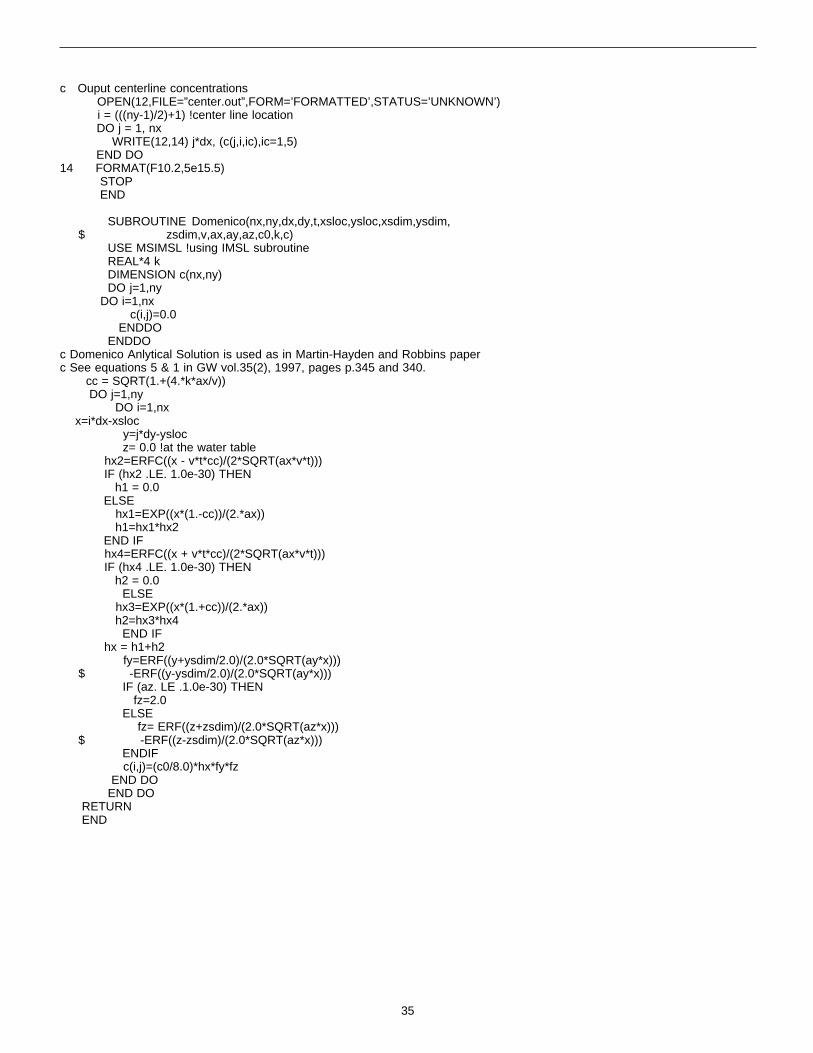
35

c Ouput centerline concentrations OPEN(12,FILE=”center.out”,FORM=’FORMATTED’,STATUS=’UNKNOWN’) i = (((ny-1)/2)+1) !center line location DO j = 1, nx WRITE(12,14) j*dx, (c(j,i,ic),ic=1,5) END DO14 FORMAT(F10.2,5e15.5) STOP END

SUBROUTINE Domenico(nx,ny,dx,dy,t,xsloc,ysloc,xsdim,ysdim, $ zsdim,v,ax,ay,az,c0,k,c)

USE MSIMSL !using IMSL subroutineREAL*4 kDIMENSION c(nx,ny)DO j=1,ny

DO i=1,nx c(i,j)=0.0 ENDDOENDDO

c Domenico Anlytical Solution is used as in Martin-Hayden and Robbins paperc See equations 5 & 1 in GW vol.35(2), 1997, pages p.345 and 340. cc = SQRT(1.+(4.*k*ax/v)) DO j=1,ny

DO i=1,nx x=i*dx-xsloc

y=j*dy-ysloc z= 0.0 !at the water table

hx2=ERFC((x - v*t*cc)/(2*SQRT(ax*v*t))) IF (hx2 .LE. 1.0e-30) THEN h1 = 0.0 ELSE hx1=EXP((x*(1.-cc))/(2.*ax)) h1=hx1*hx2 END IF hx4=ERFC((x + v*t*cc)/(2*SQRT(ax*v*t))) IF (hx4 .LE. 1.0e-30) THEN h2 = 0.0

ELSE hx3=EXP((x*(1.+cc))/(2.*ax)) h2=hx3*hx4

END IF hx = h1+h2

fy=ERF((y+ysdim/2.0)/(2.0*SQRT(ay*x))) $ -ERF((y-ysdim/2.0)/(2.0*SQRT(ay*x)))

IF (az. LE .1.0e-30) THEN fz=2.0 ELSE fz= ERF((z+zsdim)/(2.0*SQRT(az*x)))

$ -ERF((z-zsdim)/(2.0*SQRT(az*x))) ENDIF c(i,j)=(c0/8.0)*hx*fy*fz END DOEND DO

RETURN END

36

Appendix A.4

Dispersivity Estimates

Dispersion refers to the process whereby a dissolved solvent will be spatially distributed longitudinally (along thedirection of ground-water flow), transversely (perpendicular to ground-water flow), and vertically (downward) because ofmechanical mixing and chemical diffusion in the aquifer. These processes develop the “plume” shape that is the spatialdistribution of the dissolved solvent mass in the aquifer.

Selection of dispersivity values is a difficult process, given the impracticability of measuring dispersion in the field.However, dispersivity data from over 50 sites has been compiled by Gelhar et al. (1992) (see Figures A.3 and A.4). Theempirical data indicates that longitudinal dispersivity, in units of length, is related to scale (distance between source andmeasurement point). Gelhar et al. (1992) indicate 1) there is a considerable range of dispersivity values at any givenscale (on the order of 2 - 3 orders of magnitude), 2) suggest using values at the low end of the range of possibledispersivity values, and 3) caution against using a single relation between scale and dispersivity to estimate dispersivity.However, most modeling studies do start with such simple relations, and BIOCHLOR is programmed with somecommonly used relations representative of typical and low-end dispersivities.

Note: Based on Gelhar’s work, use of variable dispersivity values should yield a better estimate of concentration at eachdistance downgradient of the source. However, when using field data to calibrate the model and estimate ratecoefficients, be aware that the Domenico model assumes constant dispersivity values. The user must choose betweenusing a variable dispersivity that is likely to be more physically accurate at each point or a fixed dispersivity value thatmakes each point mathematically consistent with each other. In general, if the user would like the best estimate ofconcentration at each point in a BIOCHLOR simulation, use a variable dispersivity. If the user would like accurate massbalances between each point, use a fixed dispersivity. Fixed dispersivity values should be used for two-zonesimulations.

BIOCHLOR is programmed with some commonly used relations based on x (distance from the source in ft) that arerepresentative of typical and low-end dispersivities. The user also has the option to enter fixed diffusivity values.

• Longitudinal Dispersivity

The user is given three options:

Option 1 (the default option) allows the user to specify a fixed value for alpha x. One commonly usedrelation is to assume that alpha x is 10% of the estimated plume length.

Option 2 assumes that alpha x = 0.1* x

Option 3 calculates the longitudinal dispersivity using the following correlation:

Alpha x = 3.28 ⋅0.82 ⋅ log 10

x3.28

2.446

(Xu and Eckstein, 1995; Al-Suwaiyan, 1996)

• Transverse Dispersivity

The user may choose a ratio of alpha y : alpha x. One commonly used ratio is:

Alpha y: alpha x = 0.10 (Based on high reliability points from Gelhar et al., 1992)

• Vertical Dispersivity

The user may choose a ratio of alpha z : alpha x. One commonly used ratio is:

Alpha z: alpha x = 0.05 (ASTM, 1995)

Alternatively, alpha z :alpha x can be set to a very low number (e.g., E-99) to yield a conservative estimate of verticaldispersion. This is the default value used in BIOCHLOR.

Other commonly used relations include:

Alpha x = 0.1 Lp (Pickens and Grisak, 1981)

37

Alpha y = 0.33 alpha x (ASTM, 1995) (EPA, 1986)

Alpha z = 0.05 alpha x (ASTM, 1995)

Alpha z = 0.025 alpha x to 0.1 alpha x (U.S. EPA, 1986)

The BIOCHLOR input screen includes Excel formulas to estimate dispersivities from scale. BIOCHLOR uses themodified Xu and Eckstein (1995) algorithm for estimating longitudinal dispersivities because 1) it provides lower rangeestimates of dispersivity, especially for large values of x and 2) it was developed after weighing the reliability of thevarious field data compiled by Gelhar et al. (1992) (see Figure A.3). BIOCHLOR also employs low-end estimates fortransverse and vertical dispersivity estimates (0.10 * alpha x and 0, respectively) because these relations better fit highreliability field data reported by Gelhar et al. (see Figure A.4), and Gelhar et al. recommend use of values in the lowerrange of the observed data. The user can also enter a fixed longitudinal dispersivity value in the “Change Alpha x Calc.”dialog box on the input screen.

Note that the Domenico model and BIOCHLOR are not formulated to simulate the effects of chemical diffusion.Therefore, contaminant transport through very slow hydrogeologic regimes (e.g., clays and slurry walls) should probablynot be modeled using BIOCHLOR unless the effects of chemical diffusion are proven to be insignificant.

10-1 10 0 101 10 2 10 3 104

Scale (m)

10 5 610

10 4

10 3

10 2

10 1

10 0

10-1

10-2

10-3

RELIABILITY

Longitudinal Dispersivity= 10% of scale

Data Source: Gelhar et al., 1992

(Pickens and Grisak, 1981)

(Xu and Eckstein, 1995)

Longitudinal Dispersivity= 0.83 [Log (scale)]2.41410

Low

Intermediate

High

Figure A.3. Longitudinal dispersivity vs. scale data reported by Gelhar et al. (1992). Data includes Gelhar’s reanalysis of several dispersivitystudies. Size of circle represents general reliability of dispersivity estimates. Location of 10% of scale linear relation plotted as dashedline (Pickens and Grisak, 1981). Xu and Eckstein’s regression shown as solid line. Shaded area defines ±1 order of magnitude fromthe Xu and Eckstein regression line and represents general range of acceptable values for dispersivity estimates.

38

Appendix A.5

Pump and Treat Comparison

A useful way to estimate the clean-up time for a contaminated aquifer is to consider the number of pore volumes thatmust be pumped from the contaminated zone to achieve clean-up goals. A pump and treat module was added to theBIOCHLOR array output page to permit users to test the feasibility of pump and treat systems and to compare pump andtreat clean-up times with natural attenuation predictions.

The user is provided with the volume of ground water in the plume (i.e., a pore volume). One pore volume is only a smallfraction of the volume of ground water requiring treatment because dense non-aqueous phase liquids (DNAPLs), suchas solvents, and sorbed constituents act as continuing sources of ground-water contamination. The number of porevolumes required for clean-up (i.e., the number of times the contaminated region must be flushed) is a function of manydifferent factors including: the clean-up standard, the initial chemical concentration, the degree of mixing of clean andcontaminated ground water, geologic heterogeneities, the presence and quantity of DNAPL, and sorbed constituents(NRC, 1994).

In the pump and treat module, the user enters the system pumping rate, and the number of pore volumes treated/removed in one year is calculated by the program. This value provides the user with an indication of the feasibility ofthe pump and treat system. If the extraction rate is less than one pore volume per year, the attainment of clean-upcriteria will likely take decades, even under the most favorable conditions (NRC, 1994).

Another cell asks the user to input the number of pore volumes that must be removed in order to clean up the aquifer.Using this value and the pumping rate, the time to clean up the contaminated aquifer can be estimated. The number ofpore volumes required to remediate the aquifer is a site-specific and technology-specific value. The document,“Guidance on Remedial Actions for Contaminated Ground Water at Superfund Sites“(U.S. EPA, 1988), describes twomethods for estimating ground-water clean-up times based on the number of pore volumes: the batch flushing model andthe continuous flushing model. Neither of these methods account for DNAPL and, therefore, underestimate clean-uptimes. A third method accounting for DNAPL is reported in Newell et al. (1994) and Wiedemeier et al. (1999).

Figure A.4. Ratio of transverse dispersivity and vertical dispersivity to longitudinal dispersivity data vs. scale reported by Gelhar et al. (1992).Data includes Gelhar’s reanalysis of several dispersivity studies. Size of symbol represents general reliability of dispersivity esti-mates. Location of transverse dispersivity relation used in BIOCHLOR is plotted as dashed line.

39

Appendix A.6

BIOCHLOR Example

Example : Cape Canaveral Air Station, Fire Training Area, Florida

Problem: Determine the concentration of TCE discharging into the canal in 1998, given datacollected in 1997.

Given:

• Input Data

• Fig. A.5 Source Map

• BIOCHLOR Modeling Summary

• Fig. A.6 BIOCHLOR Input Data

Results:

• Fig. A.7 BIOCHLOR Centerline Output

• Fig. A.8 BIOCHLOR TCE Centerline Output

• Fig. A.9 BIOCHLOR TCE Array Output

40

BIOCHLOR ExampleCape Canaveral Air Station, Florida

DATA TYPE Parameter Value Source of Data

Hydrogeology • Hydraulic Conductivity:• Hydraulic Gradient:

• Effective porosity:

1.8 x 10-2 (cm/sec) 0.0012 (ft/ft)

0.2

• Slug-tests results• Static water level

measurements• Estimated

Dispersion • Longitudinal Dispersivity:

• Transverse Dispersivity:• Vertical Dispersivity:

40

40 (ft)

• Intermediate value for800-1200 ft. plume (fromGelhar et al. (1992))

• 0.1 x long. dispersivity• Assume vertical

dispersivity is zero sincedepth of source isapprox. depth of aquifer

Adsorption • Individual RetardationFactors

Common Retardation Factor• Aquifer Matrix Bulk Density• foc:• Koc:

PCE:7.1 TCE: 2.9c-DCE: 2.8 VC: 1.4ETH: 5.32.91.6 (kg/L)0.184%PCE: 426 (L/kg) TCE: 130(L/kg)c-DCE: 125 (L/kg) VC: 29.6 (L/kg)ETH: 302 (L/kg)

• Calculated from R=1+Koc•foc•ρb/n • Median value• Estimated• Lab analysis• Literature correlation

using solubilities at 20 oC

Biotransformation Biotransformation RateCoefficients, (1/yr)

PCE----> TCE

TCE---->c-DCE

c-DCE--->VC

VC-----> ETH

2.0

1.0

0.7

0.4

• Based on calibration tofield data using asimulation time of 32years (field data collectedin 1997). Started withliterature values and thenadjusted model to fitfield data

General • Modeled Area Length:• Modeled Area Width: • Simulation Time:

1085 (ft)700 (ft)

33 (yrs)

• Based on area of affectedground-water plume

• From 1965 (first release)to 1998

Source Data • Source Thickness:

• Source Widths (ft)

• Source Concentrations (mg/L)

PCE

TCE

c-DCE

VC

ETH

56(ft)

Area 1 Area 2 Area 3105 175 298

Area 1 Area 2 Area 30.056 0.007 0.001

15.8 0.316 0.01

98.5 1.0 0.01

3.080 0.089 0.009

0.030 0.013 0.003

• Based on geologic logsand monitoring data (seefigure A.5 for TCEExample)

• Modeled source area asvariable source

• Source concentrations areaqueous concentrations

Actual Data Distance From Source (ft):

PCE Conc. (mg/L):

TCE Conc. (mg/L)

c-DCE (mg/L)

VC (mg/L)

ETH (mg/L)

560 650 930 1085

<0.001 ND <0.001 <0.001

0.220 0.0165 0.0243 0.019

3.48 0.776 1.200 0.556

3.080 0.797 2.520 5.0240.188 ND 0.107

0.150

• Based on 1997 observedconcentrations at sitenear centerline of plume

OUTPUT Centerline Concentration: See Figures A.7, A.8

Array Concentration: See Figure A.9

41

MP-5< 0.001

MP-60.024

CPT-6

MP-20.044

MP-30.220

CPT-7ND

CPT-40.017

CPT-90.004

CCFTA2-21S0.003

CCFTA2-20S0.008

CCFTA2-140.042

MP-4S0.019

CCFTA2-30.030

CCFTA2-50.003

CCFTA2-20.001

CCFTA2-10.001

CCFTA2-10ND

CCFTA2-11ND

CCFTA2-9S 15.8

CCFTA2-18< 0.001

CCFTA2-4< 0.001

CCFTA2-6< 0.001

CPT-1ND

CCFTA2-7S3.6

C a n a l

B a n a n a

R i v e r

1 23

SCALE (ft.)

0 150 300

298

ft

175

ft

105

ft

1.0

0.001

0.010

0.100

CCFTA-2, Cape Canaveral Air Station, Florida

LEGEND

FIGURE A.4

Monitoring point

Monitoring well location

TCE detected in groundwater sample, mg/L0.003

No TCE detectedND

SourceZone

1

23

Width (ft)Actual Source Conc.

in 1997 (mg/L)

105

175298

15.8

TCE concentration isopleth, mg/L

BIOCHLOR SOURCE ZONE ASSUMPTIONS

(TCE AS EXAMPLE)

This method of determining widths is different from the method used in BIOSCREEN.

1.0

Source Zone Assumption

NOTE:

0.3160.01

How Derived

Maximum concentration

Geometric mean between edge of zone 2 and 3Geometric mean between edge of zone 1 and 2

Figure A.5. BIOCHLOR source zone assumptions (TCE as example).

42

BIOCHLOR Modeling Summary,

Cape Canaveral Air Station, FloridaEntering Input• BIOCHLOR was used to reproduce the movement of the plume from 1965 (the best guess for when the release

occurred) to 1998.

• The hydraulic conductivity, hydraulic gradient, and the effective porosity were entered and the “C” button waspressed to generate the seepage velocity.

• For longitudinal dispersivity, a fixed dispersivity of 40 ft (Option 1) was chosen. The ratio of lateral dispersivity tolongitudinal dispersivity was set to 0.1 and the vertical dispersivity was set to 0. This last value was chosen becausethe depth of the source area is similar to the depth of the saturated zone.

• To determine the retardation factors, the aquifer matrix bulk density, the partition coefficients at 20oC, and thefraction of organic carbon were input into the gray cells and the “C” button was pushed to yield the retardation factors.BIOCHLOR uses one retardation factor, not individual retardation factors for each constituent. The default value forthe common retardation factor is the median retardation factor, but the user can over-ride this value. In cases wherethe retardation factor varies significantly among the constituents, it is advisable to do a sensitivity analysis todetermine how the choice of the common R affects the model predictions. For this simulation, the median value of2.85 was chosen.

• For modeling biotransformation, the user has the choice of modeling the plume in one or two zones. Modeling in twozones permits the use of a different set of rate coefficients in each zone, but requires that the plumes be at steadystate (as established from field data). In this example, we will model the plume as one anaerobic zone using one setof rate coefficients. (Field dissolved oxygen, ORP, and geochemical data were used to establish anaerobicconditions.) Because field-scale rate coefficients and rate data from microcosms were unavailable, rate coefficientspreviously obtained by calibrating the model to 1997 field data were used. Here, the rate coefficients were enteredinto the white cells.

• In the General Section, the model area length, width, and simulation time must be entered. The model area lengthis the distance from the source to the receptor (the canal, in this case study). A width of 700 ft is chosen to besignificantly larger than the plume width to capture all of the mass discharging into the canal. A simulation time of33 years was chosen because the simulation is being conducted for 1998, and the solvents were released startingin 1965.

• Because we are interested in centerline predictions and the mass flux into the canal, the source area will be modeledas a spatially-variable source. By pressing the “Source Options” button and selecting “Spatially-Variable Source”, adialog box pops up that allows for the input of source area concentration and width data. To obtain the mostconservative centerline predictions, the maximum concentration in the source area were used for zone 1. The othertwo concentrations were obtained by taking the geometric means between adjacent isopleths (see Figure A.5).Once these data are entered and “OK” is pressed, the data are transferred to the input page and you will see thelayout shown in Figure A.6. Note that any subsequent changes to the source area concentrations can be donedirectly on the input page without going through the dialog box. Lastly, the thickness of the source area wasdetermined by entering the deepest depth where chlorinated solvents were detected in the aqueous phase.

• Finally, there is an input area for field data. In this example, the 1997 field data were used (previously) to determinethe rate constants provided. If one does not have field-scale rate constants or rate data from microcosm studies,these values become important for calibrating the model.

Viewing Output• There are two choices for viewing the output. Centerline predictions are shown for all five species in Figure A.6 and

for TCE in Figure A.8. Figure A.7 shows the centerline predictions for each chlorinated solvent and a no degradationcurve for all of the chlorinated solvents added together as well as field data. From this screen, the user can view thecenterline predictions of each constituent individually or go to the array screen. Figure A.8 shows the centerlineprediction for TCE, with and without biotransformation. However, any of the constituents can be viewed by pressingthe buttons to the right of the graph. Here we can see that the TCE concentration discharging into the canal (at1085 ft) is 0.003 mg/L.

43

• From this screen or from the input screen the array page can be selected. The array output for this problem isdisplayed in Figure A.9. This three-dimensional figure shows the longitudinal and lateral extent of contamination.Again, the user can select the constituent to be viewed and the no degradation or biotransformation prediction. Notethat the scale on the array automatically changes depending on the magnitude of the concentrations. These arrayvalues are maximum values because the array is evaluated at z=0.

Other information that is presented on the output screen includes the mass removed, the percent biotransformed, andthe mass flux. The TCE mass flux discharging to the canal is approximately 83 mg/day.

Figure A.6. BIOCHLOR input screen. Cape Canaveral Air Force Base, Florida.

44

Figure A.7. Centerline output. Cape Canaveral Air Force Base, Florida.

Figure A.8. Individual centerline output for TCE, Cape Canaveral Air Station, Florida.

45

Figure A.9. Array concentration output for TCE. Cape Canaveral Air Station, Florida.

46

Sensitivity Analysis Examples

Sensitivity analyses are recommended when literature values are used or if there is uncertainty in an input parameter.To illustrate the response of the BIOCHLOR model to changes in the input parameters, a sensitivity analysis wasconducted for the first order decay coefficients and also for the common retardation factor.

In the first sensitivity analysis example, the case study (baseline) problem was run with the same input parametersexcept that the first order decay coefficients were multiplied by 2. Similarily, another simulation was conducted wherebythe rate coefficients were 0.1 times those used in the baseline example. The centerline concentrations of PCE, TCE andthe daughter products 1085 ft downgradient from the source are shown in Table A.4 for each simulation. In this instance,the simulated concentrations of PCE and its daughter products increase substantially when the rate coefficient isdecreased by a factor of ten and doubling the rate coefficient decreases the chlorinated solvent concentrations at thecanal location. In this example, the chlorinated ethene concentrations are very sensitive to the magnitude of the ratecoefficient.

TableA.4. Sensitivity Analysis Results - Rate Coefficients

Constituent Concentrations

(mg/L)2X Baseline Baseline * 0.1X Baseline

PCE 0.000 0.000 0.006

TCE 0.000 0.003 2.254

DCE 0.003 0.202 19.443

VC 0.137 2.039 8.819

baseline λPCE→TCE

=2.00 yr-1, λTCE→DCE

=1.00 yr-1, λDCE→VC

=0.70 yr-1, λVC→ETH

=0.40 yr-1

In contrast, changes in the retardation factor have nominal effects on the dissolved chlorinated solvent concentrations asshown in Table A.5. In this sample case, when the retardation factor is decreased from the baseline value of 2.9,chlorinated solvent concentrations increase slightly. Also, with an increase in the retardation factor chlorinated solventconcentrations at the canal location decrease by a small amount. These small variations in the concentrations due to thechanges in the retardation factor can probably be attributed to the plume being near steady-state in this example.

Table A.5. Sensitivity Analysis Results - Retardation Factor

Constituent Concentrations (mg/L)

R=1.4 R=2.8 (Baseline ) R=4.7

PCE 0.000 0.000 0.000

TCE 0.003 0.003 0.003

DCE 0.204 0.202 0.112

VC 2.161 2.039 0.798

In this example, the BIOCHLOR model is more sensitive to changes in the first-order decay coefficient and less sensitiveto changes in the retardation factor. However, the results of these sensitivity analyses are site-specific and do not applyto all sites.