a

REPORT OF EXPERTS WORKSHOP (HOBART, SEPTEMBER 2006)

BIOREGIONALISATIONOF THE SOUTHERN OCEAN

Acknowledgements:

This report presents the outcomes of an Experts Workshop on Bioregionalisation of the Southern Ocean, held in Hobart, Australia, 4-8 September 2006, hosted by WWF-Australia and the Antarctic Climate and Ecosystems Cooperative Research Centre.

This workshop, and the preparation and publication of the report, was made possible through the generous support of Peregrine Adventures, which operates expedition-style voyages to the Antarctic Peninsula, the Falkland Islands and South Georgia. Peregrine supports WWF-Australia with funds raised through passenger and staff donations on board their ships, the Peregrine Mariner and Peregrine Voyager.

Responsible Tourism is a fundamental platform of Peregrine’s operations. In line with this principle of sustainability, Peregrine has funded this report in the belief that it provides a foundation for the understanding and long-term conservation of Antarctica’s important habitats and wildlife.

Additional support was provided throughout the project by WWF-Australia and the Antarctic Climate and Ecosystems Cooperative Research Centre.

The authors wish to thank all of the participants in the 2006 Experts Workshop, whose expertise and thoughtful input provided the material and outcomes for this report, as well as reviews of the manuscript. A full list of participants can be found at the end of the report.

Cover photo: © Paul Dudley courtesy Australian Government Antarctic Division

For copies of this report please contact:

WWF-Australia Head Offi ceGPO Box 528Sydney, NSW, Australia 2001Tel: +612 9281 5515wwf.org.au

© WWF-Australia and Antarctic Climate and Ecosystems Cooperative Research Centre (ACE CRC). All rights reserved. 2006.

All material appearing in this publication is copyrighted and may be reproduced with permission. Any reproduction in full or in part of this publication must credit WWF and ACE CRC as the copyright owners.

The views expressed in this publication are those of the authors and do not necessarily represent the views of WWF or ACE CRC.

Report prepared by: Susie Grant, Andrew Constable, Ben Raymond and Susan Doust. Additional contributing authors: Roger Hewitt, Harry Keys, John Leathwick, Vincent Lyne, Rob Massom, Matt Pinkerton, Ben Sharp and Phil Trathan.

This report should be cited as:Grant, S., Constable, A., Raymond, B. and Doust, S. (2006) Bioregionalisation of the Southern Ocean: Report of Experts Workshop, Hobart, September 2006. WWF-Australia and ACE CRC.

The CD attached to this report includes appendices, analysis tools, data and maps (including a GIS database) referred to in the report.

ISBN: 1 921031 16 6

Way

ne P

apps

, Aus

tral

ian

Gov

ernm

ent A

ntar

ctic

Div

isio

n, ©

Com

mon

wea

lth o

f Aus

tral

ia

1

Table of ContentsAcknowledgements

Acronyms and abbreviations

Table of Contents

Executive Summary

1. Introduction

1.1 What is bioregionalisation?

Defi ning regions

1.2 Bioregionalisation in the Antarctic context

CCAMLR

Committee for Environmental Protection

1.3 Antarctica and the Southern Ocean

Southern Ocean characteristics

Existing regionalisations for the Southern Ocean

1.4 Experts Workshop

2. Approach to bioregionalisation

2.1 Identifying properties to be captured

2.2 Classifi cation method

Choosing clustering algorithms

2.3 Variables that capture properties

2.4 Uncertainty

3. Physical regionalisation

3.1 Summary of adopted method

Primary regionalisation

Secondary regionalisation

3.2 Results of Southern Ocean bioregionalisation

Primary regionalisation

Uncertainty

Secondary regionalisation

3.3 Expert review of bioregionalisation results

South Atlantic (Area 48)

Indian Ocean (Area 58)

Pacifi c Ocean (Area 88)

4. Future work

5. Conclusion

List of Appendices (provided on CD)

List of workshop participants

Glossary of terms

References

Acronyms and abbreviations

ACC Antarctic Circumpolar Current

ATCM Antarctic Treaty Consultative Meeting

CCAMLR Commission for the Conservation of

Antarctic Marine Living Resources

CEP Committee for Environmental Protection

CPR Continuous Plankton Recorder

LME Large Marine Ecosystem

MPA Marine Protected Area

PAR Photosynthetically active radiation

PF Polar Front

SACCF Southern Antarctic Circumpolar Current Front

SAF Subantarctic Front

SC-CAMLR Scientifi c Committee for the Conservation of

Antarctic Marine Living Resources

SSH Sea surface height

SST Sea surface temperature

STF Subtropical Front

2

Pho

togr

aph

by W

ayne

Pap

ps, A

ustr

alia

n G

over

nmen

t Ant

arct

ic D

ivis

ion

© C

omm

onw

ealth

of A

ustr

alia

3

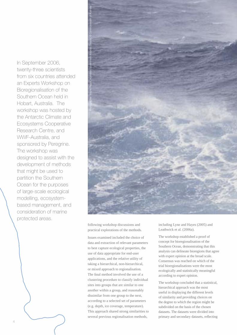
In September 2006, twenty-three scientists from six countries attended an Experts Workshop on Bioregionalisation of the Southern Ocean held in Hobart, Australia. The workshop was hosted by the Antarctic Climate and Ecosystems Cooperative Research Centre, and WWF-Australia, and sponsored by Peregrine. The workshop was designed to assist with the development of methods that might be used to partition the Southern Ocean for the purposes of large-scale ecological modelling, ecosystem-based management, and consideration of marine protected areas. In 2005, the Commission for the Conservation of Antarctic Marine Living Resources (CCAMLR) and its Scientifi c Committee (SC-CAMLR) considered that a bioregionalisation of the Southern Ocean was needed to underpin the development of a system of marine protected areas in the Convention area.

The aim of the workshop was to bring together scientifi c experts in their independent capacity to develop a ‘proof of concept’ for a broad-scale bioregionalisation of the Southern Ocean, using physical environmental data and satellite-measured chlorophyll concentration as the primary inputs. Work included presentation of background information, computer-based analysis undertaken in small groups, and plenary discussion on the methods, data and results. Workshop participants are listed at the end of this report.

At the conclusion of the workshop, a method had been agreed upon that could be used to take the bioregionalisation work forward. Consensus was achieved on a draft physical regionalisation, and progress was made in determining how to include additional (e.g. biological) data for a more complete bioregionalisation. This report outlines the key results of the workshop, and highlights some of the issues discussed.

An understanding of the spatial characteristics of large ecosystems such as the Southern Ocean is important for the achievement of a range of scientifi c, conservation and management objectives. Bioregionalisation is a process that aims to partition a broad spatial area into distinct spatial regions, using a range of environmental and biological information. The process results in a set of bioregions, each with relatively homogeneous and

predictable ecosystem properties. The properties of a given bioregion should differ from those of other regions in terms of species composition as well as the attributes of its physical and ecological habitats.

Classifi cation of regions based only on biological data is often impractical at larger scales because of insuffi cient geographic coverage, even though there may be suffi cient data to subdivide smaller-scale portions of those regions. Physical and satellite-observed data generally have better spatial and temporal coverage and greater availability than biological data. These can be used to help characterise regions on the basis of environmental properties, physical processes, primary production, and habitat type.

Initial discussions during the workshop focused on defi ning the major physical processes in the Southern Ocean, and their relationships with ecological processes. A key aspect of undertaking an ecologically meaningful regionalisation is to understand how important ecological processes correspond to the physical and satellite-observed parameters, and whether these parameters are appropriate for use as proxies or surrogates. This may depend in part on the end-use application of the analysis, and the scale at which the analysis is being undertaken.

Environmental data used as the primary input for analysis during this workshop were chosen based on their spatial coverage across the Southern Ocean. The datasets considered included bathymetry, sea ice concentration and extent, sea surface temperature, sea surface height, chlorophyll a concentration, nutrient data (silicate, nitrate and phosphate), and insolation (photosynthetically active radiation - PAR).

A series of presentations on approaches to bioregionalisation that have been undertaken elsewhere (terrestrial Antarctica, Australia, New Zealand) allowed detailed consideration of the relative benefi ts of different methods. The analytical methods used by Lyne and Hayes (2005), Leathwick et al. (2006a) and Raymond & Constable (2006) were used as starting points for the analysis during the workshop. These methods were refi ned into a single methodology,

Executive Summary

4

following workshop discussions and

practical explorations of the methods.

Issues examined included the choice of

data and extraction of relevant parameters

to best capture ecological properties, the

use of data appropriate for end-user

applications, and the relative utility of

taking a hierarchical, non-hierarchical,

or mixed approach to regionalisation.

The fi nal method involved the use of a

clustering procedure to classify individual

sites into groups that are similar to one

another within a group, and reasonably

dissimilar from one group to the next,

according to a selected set of parameters

(e.g. depth, ice coverage, temperature).

This approach shared strong similarities to

several previous regionalisation methods,

including Lyne and Hayes (2005) and Leathwick et al. (2006a).

The workshop established a proof of concept for bioregionalisation of the Southern Ocean, demonstrating that this analysis can delineate bioregions that agree with expert opinion at the broad scale. Consensus was reached on which of the trial bioregionalisations were the most ecologically and statistically meaningful according to expert opinion.

The workshop concluded that a statistical, hierarchical approach was the most useful in displaying the different levels of similarity and providing choices on the degree to which the region might be subdivided on the basis of the chosen datasets. The datasets were divided into primary and secondary datasets, refl ecting

In September 2006, In September 2006, twenty-three scientists twenty-three scientists from six countries attended from six countries attended an Experts Workshop on an Experts Workshop on Bioregionalisation of the Bioregionalisation of the Southern Ocean held in Southern Ocean held in Hobart, Australia. The Hobart, Australia. The workshop was hosted by workshop was hosted by the Antarctic Climate and the Antarctic Climate and Ecosystems Cooperative Ecosystems Cooperative Research Centre, and Research Centre, and WWF-Australia, and WWF-Australia, and sponsored by Peregrine. sponsored by Peregrine. The workshop was The workshop was designed to assist with the designed to assist with the development of methods development of methods that might be used to that might be used to partition the Southern partition the Southern Ocean for the purposes Ocean for the purposes of large-scale ecological of large-scale ecological modelling, ecosystem-modelling, ecosystem-based management, and based management, and consideration of marine consideration of marine protected areas.protected areas.

Pho

togr

aphe

r: W

ayne

Pap

ps, A

ustr

alia

n G

over

nmen

t Ant

arct

ic D

ivis

ion,

© C

omm

onw

ealth

of A

ustr

alia

5

the primary properties of the region and the secondary environmental properties that might provide smaller-scale subdivisions to refl ect the spatial heterogeneity of the Southern Ocean ecosystem.

The primary datasets used in this analysis were depth, sea surface temperature, silicate and nitrate. These highlighted the different environmental characteristics of large regions including the continental shelf and slope, frontal features (Subantarctic Front, Polar Front, Southern Antarctic Circumpolar Current Front), the deep ocean, banks and basins, island groups and gyre systems. Other primary datasets that could be usefully considered in future analyses were identifi ed by the workshop, and included sea surface height and insolation.

The secondary datasets used in the analysis were ice concentration and mean chlorophyll a values. The addition of these datasets suggested smaller-scale spatial heterogeneity within the regions particularly in the continental shelf and slope areas, and the seasonal ice zone. These results highlighted the need for further analysis at the secondary level.

The fi nal stages of the analysis included discussion on how well the defi ned regions corresponded to our present knowledge of the Southern Ocean. Experts provided information on the patterns and features that they would expect to see, according to current observations and understanding, and these largely concurred with the outcomes of the analysis.

Finally, workshop participants discussed priorities for future work, including the development of further methods to deal with uncertainty, understanding of inter- and intra-annual variation, validation of results, the incorporation of additional data (particularly biological datasets) and fi ner-scale analysis of particular areas of interest.

This workshop established a ‘proof of concept’ for bioregionalisation of the Southern Ocean. Continuation of this work will be an important contribution to the achievement of a range of scientifi c, management and conservation objectives, including large-scale ecological modelling, ecosystem-based management, and the development of an ecologically representative system of marine protected areas.

6

1. Introduction

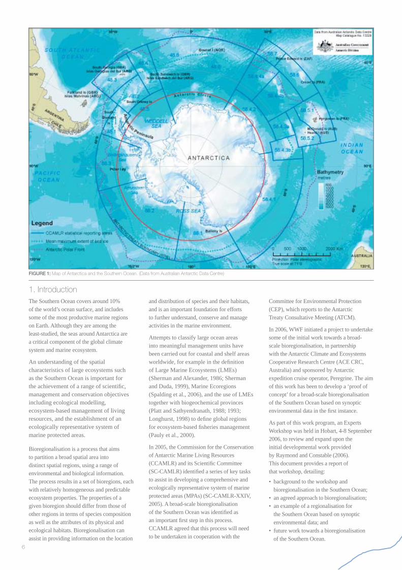
FIGURE 1: Map of Antarctica and the Southern Ocean. (Data from Australian Antarctic Data Centre)

The Southern Ocean covers around 10% of the world’s ocean surface, and includes some of the most productive marine regions on Earth. Although they are among the least-studied, the seas around Antarctica are a critical component of the global climate system and marine ecosystem.

An understanding of the spatial characteristics of large ecosystems such as the Southern Ocean is important for the achievement of a range of scientifi c, management and conservation objectives including ecological modelling, ecosystem-based management of living resources, and the establishment of an ecologically representative system of marine protected areas.

Bioregionalisation is a process that aims to partition a broad spatial area into distinct spatial regions, using a range of environmental and biological information. The process results in a set of bioregions, each with relatively homogeneous and predictable ecosystem properties. The properties of a given bioregion should differ from those of other regions in terms of species composition as well as the attributes of its physical and ecological habitats. Bioregionalisation can assist in providing information on the location

and distribution of species and their habitats, and is an important foundation for efforts to further understand, conserve and manage activities in the marine environment.

Attempts to classify large ocean areas into meaningful management units have been carried out for coastal and shelf areas worldwide, for example in the defi nition of Large Marine Ecosystems (LMEs) (Sherman and Alexander, 1986; Sherman and Duda, 1999), Marine Ecoregions (Spalding et al., 2006), and the use of LMEs together with biogeochemical provinces (Platt and Sathyendranath, 1988; 1993; Longhurst, 1998) to defi ne global regions for ecosystem-based fi sheries management (Pauly et al., 2000).

In 2005, the Commission for the Conservation of Antarctic Marine Living Resources (CCAMLR) and its Scientifi c Committee (SC-CAMLR) identifi ed a series of key tasks to assist in developing a comprehensive and ecologically representative system of marine protected areas (MPAs) (SC-CAMLR-XXIV, 2005). A broad-scale bioregionalisation of the Southern Ocean was identifi ed as an important fi rst step in this process. CCAMLR agreed that this process will need to be undertaken in cooperation with the

Committee for Environmental Protection (CEP), which reports to the Antarctic Treaty Consultative Meeting (ATCM).

In 2006, WWF initiated a project to undertake some of the initial work towards a broad-scale bioregionalisation, in partnership with the Antarctic Climate and Ecosystems Cooperative Research Centre (ACE CRC, Australia) and sponsored by Antarctic expedition cruise operator, Peregrine. The aim of this work has been to develop a ‘proof of concept’ for a broad-scale bioregionalisation of the Southern Ocean based on synoptic environmental data in the fi rst instance.

As part of this work program, an Experts Workshop was held in Hobart, 4-8 September 2006, to review and expand upon the initial developmental work provided by Raymond and Constable (2006). This document provides a report of that workshop, detailing:

• background to the workshop and bioregionalisation in the Southern Ocean;• an agreed approach to bioregionalisation;• an example of a regionalisation for the Southern Ocean based on synoptic environmental data; and• future work towards a bioregionalisation of the Southern Ocean.

7

An understanding of the spatial characteristics of large ecosystems such as the Southern Ocean is important for the achievement of a range of scientifi c, conservation and management objectives. Bioregionalisation is a process that aims to partition a broad spatial area into distinct spatial regions, using a range of environmental and biological information. The process results in a set of bioregions, each with relatively homogeneous and predictable ecosystem properties. The properties of a given bioregion should differ from those of other regions in terms of species composition as well as the attributes of its physical and ecological habitats.

Large ecosystems can be partitioned at a range of spatial scales, according to their physical, environmental and biological characteristics. Variation in climate, topography and other physical factors forms different habitat types, which in turn support different species and communities. Biological diversity varies throughout this geographic space, and may be further infl uenced byfactors such as the availability of nutrients and food, as well as human activities.

For example, forests, deserts and grasslands have different physical and environmental attributes, and contain different habitat types and communities of species. These different regions may occur adjacent to one another; however, each differs from the others in terms of physical and ecological characteristics. Some species may range across more than one region, whereas others will be more restricted in their range, according to their ability to live in particular habitat types or ecological conditions. For example, cacti are uniquely adapted to live only in desert conditions, while certain ubiquitous grasses are found in parts of the forest and the grassland, as well as the desert. Migrating birds may travel across all three regions, while deer inhabit the forest and the grassland but not the desert, and tree-dwelling mammals remain exclusively in the forest.

Boundaries between regions may be sharp, for example at the interface between a forest and adjacent alpine areas. Features such as the tree-line refl ect the limit of tolerance by

certain species to a particular set of physical conditions. However, boundaries may also be gradual, such as in the margins of a desert, where habitats and species from both the desert and the neighbouring grassland gradually blend across a wide transitional area. Transitional areas between adjacent ecosystems, regions or habitats are known as ecotones, and species may be found in decreasing numbers as they reach the edge of their range. Bioregionalisation provides a simplifi ed interpretation of these physical and ecological boundaries. It endeavours to separate, say, desert, grassland and forest by drawing boundaries between them such that the attributes within each of the bounded areas are primarily desert, grassland and forest respectively.

This terrestrial analogy provides a simplifi ed description of the bioregionalisation concept, and its utility in providing pragmatic solutions to complex ecological problems. Apart from the edges of rocky reefs, regional boundaries in the oceans are likely to be less sharp (or more ‘fuzzy’), and they may be more mobile or variable because of the fl uid nature of the marine environment. Regionalisation of marine ecosystems is also more complex because of their three-dimensional nature. However, marine ecosystems can nevertheless be partitioned using the principles described above to provide a simplifi ed interpretation spatial differences in their environmental characteristics, habitat types and ecological boundaries.

1.1 What is bioregionalisation?

8

Regions are generally defi ned using a

combination of qualitative (expert opinion,

descriptive data) and quantitative statistical

analyses. A range of data on physical,

environmental and biological properties

can be incorporated into a regionalisation

analysis, according to data availability and

coverage, and specifi c end-use applications.

Statistical procedures for undertaking a

regionalisation attempt to partition a broad

spatial area into discrete regions, each with

relatively homogeneous and predictable

ecosystem properties, but sometimes

occurring in more than one geographic

location (Leathwick et al. 2003). The

properties of a given region (both species

composition as well as attributes of the

physical and ecological habitats) should

differ from those of adjacent regions.

Regions can be defi ned according to the

range of species or communities that

inhabit them. Indicator species may also be

used, where individual species are known

to exclusively inhabit a certain type of

region. For example, certain species of

desert snake, grassland lizard and forest

frog might be used as indicators to defi ne

these regions.

Alternatively, physical and environmental

information can be used to defi ne regions

using qualitative methods (e.g. Bailey,

1996). Topography, altitude, substratum

and temperature are among the variables

which infl uence the characteristics and

structure of habitats and their associated

species and communities. An understanding

of the spatial extent of different

environmental conditions and physical

habitats can provide further information

on the ecological properties likely to be

found in each area, and thus the types

of communities or species which might

occur there. As a simplifi ed example, the

distribution of freshwater habitats may give

some indication of where frogs are likely to

be found. This is particularly useful where

biological information is unavailable.

Information on the distribution of frogs

over a large area may be impractical to

obtain, however freshwater ponds could

Defi ning regions

9

be more easily identifi ed using aerial photography.

Approaches to defi ning regions may also vary according to the particular application of a bioregionalisation analysis. For example, a manager interested in the conservation of reptiles may choose to defi ne regions according specifi cally to the distribution of snakes and lizards, whereas an agricultural scientist might be more interested in the division of regions according to substratum type and topography.

Bioregions may also be defi ned at different spatial scales, according to the biological, physical or environmental characteristics of interest, and the scale of the data being used in the analysis (e.g. Bailey, 1996). The forest,

grassland and desert may be encompassed within a much larger unit; for example all of these regions would be found in southern Africa. Within a particular region, there may also be fi ner-scale ecosystem divisions. For example, within a forest region, a mountain will support different vegetation with increasing altitude. Different forest communities may be found higher up the mountain, refl ecting changes in topography and climatic conditions. At an even fi ner scale, features such as mountain streams, valleys and rocky outcrops may result in different forest communities occurring at the same altitude. Smaller scale ecosystems or regions can be seen as nested within ecosystems of a higher order, thus occurring within a hierarchical system.

Clearly, the fi nal regionalisation will be

dictated by the spatial detail required

and the specifi c attributes needing to be

captured in the subdivision. Nevertheless,

a regionalisation needs to show generally

how those attributes are nested within the

larger scale heterogeneity of the system.

This helps to appreciate whether areas with

similar properties but separated in space

may be infl uenced by different external

environmental and ecological drivers at

their boundaries.

Approaches to bioregionalisation in the

marine environment have included the

use of physical oceanographic parameters

(e.g. ocean water masses, fronts, gyres

Pho

togr

aph

by W

ayne

Pap

ps, A

ustr

alia

n G

over

nmen

t Ant

arct

ic D

ivis

ion

© C

omm

onw

ealth

of A

ustr

alia

10

and wave energy), geomorphology (e.g. depth, substratum, sediment characteristics and disturbance regimes), biological oceanography (e.g. primary and secondary production), fi sh stock distribution and abundance (e.g. areas of aggregation and fi shing patterns), benthic communities (e.g. distribution and community structure) and marine mammals and birds (e.g. primary feeding and breeding locations).

Classifi cation of regions based only on biological data is often impractical at larger scales because of insuffi cient geographic coverage, even though there may be suffi cient data to subdivide smaller-scale portions of those regions (Belbin, 1993). Physical and satellite-observed data generally have better spatial and temporal

coverage and greater availability than biological data. These can be used to help characterise regions on the basis of environmental properties, physical processes, primary production, and habitat type.

An important aspect of undertaking an ecologically meaningful regionalisation is therefore to understand how important ecological processes correspond to physical parameters, and whether those parameters are appropriate for use as proxies or surrogates. This may not require much ecological detail in the fi rst instance, since physical and environmental data can provide an understanding of environmental heterogeneity which will inevitably affect the ecology of a region.

1.2 Bioregionalisation in the Antarctic context

Bioregionalisation of the Southern Ocean has relevance in a variety of applications within different scientifi c fi elds and for conservation and management across the Antarctic Treaty System. An understanding of spatial ecosystem characteristics is necessary to achieve a range of objectives in the Antarctic context, including:

• ecosystem modelling;• ecosystem-based management of marine living resources;• effective and systematic planning and management of other human activities;• identifi cation of biodiversity units and areas of high conservation value;• establishment of a comprehensive and ecologically representative system of MPAs; and• directing further research.

Recent discussions within the CCAMLR Scientifi c Committee (SC-CAMLR-XXIV) and the Committee for Environmental Protection (CEP IX) have agreed the importance of undertaking a bioregionalisation of the Southern Ocean, and highlighted the need to work together in achieving this common objective.

CCAMLRThe Convention on the Conservation of Antarctic Marine Living Resources (CCAMLR) applies to all marine living resources within the area south of a line approximating to the Polar Front. The Convention Area is divided into three sectors corresponding to the adjacent Atlantic, Indian and Pacifi c oceans. These sectors are referred to as Statistical Areas 48, 58 and 88

respectively, and each is further divided into statistical subareas for catch reporting and management purposes (see Figure 1). Statistical subareas were defi ned on the basis of ocean characteristics, fi sh stock distributions and the location of fi shing activities (Everson, 1977; Kock, 2000), thus providing one example of an existing bioregionalisation of the Southern Ocean. Subareas are used in catch reporting, and enable the implementation of conservation and management measures regionally or for individual stocks.

The primary objective of CCAMLR is the conservation of Antarctic marine living resources, where conservation includes rational use. CCAMLR has pioneered a precautionary, ecosystem approach to marine living resource management, and defi nes the Antarctic marine ecosystem as “the complex of relationships of Antarctic marine living resources with each other and with their physical environment”.1

In 2005, the CCAMLR Workshop on MPAs considered the scientifi c work required for development of a system of protected areas to assist CCAMLR in achieving its conservation objectives. A broad-scale bioregionalisation of the Southern Ocean was identifi ed as an important fi rst step in this process (SC-CAMLR-XXIV, 2005).

CCAMLR has identifi ed a series of key tasks to be undertaken towards bioregionalisation:

• collation of existing data, including benthic and pelagic features and processes;

• determination of statistical analyses required to facilitate a bioregionalisation, including use of empirical, model and expert data;• development of a broad-scale bioregionalisation of the Southern Ocean, based on existing datasets; and• delineation of fi ne-scale provinces within regions, where possible.

As part of this ongoing work, CCAMLR will hold a workshop in 2007 with the aim of providing advice on a bioregionalisation of the Southern Ocean, including, where possible, advice on smaller-scale delineation of provinces and potential areas for protection to further the conservation objective of CCAMLR. This workshop will involve members of both the CCAMLR Scientifi c Committee and the CEP, as well as external experts (SC-CAMLR-XXIV, 2005).

Committee for Environmental ProtectionThe Antarctic Treaty and its Protocol on Environmental Protection apply to the area south of 60°S, thus covering a smaller marine area than CCAMLR. The Environmental Protocol deals with environmental impact assessment, conservation of Antarctic fl ora and fauna, waste disposal and management, prevention of marine pollution, and area protection and management. The Committee for Environmental Protection (CEP) provides advice and recommendations to the ATCM in connection with the implementation of the Environmental Protocol.

Pho

togr

aph

© R

oger

Kirk

woo

d, c

ourt

esy

Aus

tral

ian

Gov

ernm

ent A

ntar

ctic

Div

isio

n

11

Annex V of the Environmental Protocol states that Parties shall seek to identify a series of Antarctic Specially Protected Areas (ASPAs) (including marine and terrestrial areas) within a ‘systematic environmental-geographic framework’2. This term has been defi ned as: “a method of classifying or organising subsets of environmental and geographic characteristics such as different types of ecosystems, habitat, geographic area, terrain, topography, climate, individual features and human presence into geographic regions. Each region would be distinctive or in some way different from other regions but some might have characteristics in common.” (ATCM XXIV/WP012, 2001).

The bioregionalisation work proposed by CCAMLR corresponds closely to current efforts by the CEP to elaborate a systematic environmental-geographic framework, in particular through the terrestrial Antarctic Environmental Domains Analysis being undertaken by New Zealand for the Antarctic continent (Morgan et al., 2005).

In outlining the work programme for bioregionalisation, CCAMLR recognised the relative expertise of the CEP, and suggested that the CEP should be invited to undertake the initial work necessary to develop a bioregionalisation of the coastal provinces, as an extension of its terrestrial bioregionalisation work. At its meeting in 2006, the CEP undertook to engage fully with CCAMLR on this work, and agreed on the importance of such an analysis in contributing to its conservation and management objectives (CEP IX, 2006).

Southern Ocean characteristics The Southern Ocean extends across a total area of almost 35 million km2, and consists of distinct provinces that differ physically and chemically (e.g. temperature, sea ice, nutrients and currents), as well as ecologically. It is characterised by deep basins, separated by large, mid-oceanic ridges and containing prominent plateaus and island groups.

Two major currents dominate the Southern Ocean system. The Antarctic Circumpolar Current (ACC) (or “West Wind Drift”) fl ows eastwards around the continent, driven by the prevailing westerly winds. The ACC forms a unique link connecting all of the world’s major oceans through an unbroken water mass surrounding the Antarctic continent, (Orsi et al., 1995). However, its path is infl uenced by topographic features such as the Kerguelen Plateau and the Scotia Arc, which defl ect fronts and generate eddies. Closer to the continent, easterly winds form a series of clockwise gyres (the largest of these being in the Ross Sea and Weddell Sea) that combine to form the westward fl owing Antarctic Coastal Current, also known as the “East Wind Drift”.

The Subtropical Front (STF) marks the northernmost extent of the ACC, separating warmer, more saline subtropical waters from fresher, cooler subantarctic surface waters (Orsi et al., 1995). Further south, the majority of ACC water is transported in the Subantarctic Front (SAF), and also in the Polar Front, which marks the transition to very cold and relatively fresh Antarctic

1.3 Antarctica and the Southern Ocean

1 CCAMLR, Article 12 Protocol on Environmental Protection, Annex V, Article 3(2)

12

FIGURE 2: Three-dimensional structure of water masses, showing relationship between the ACC and deep water (Figure reprinted with permission from: Rintoul, 2000).

Surface Water, and separates Southern Ocean waters from the Atlantic, Pacifi c and Indian oceans to the north. The Polar Front also marks the northerly limit of many non-migrating Antarctic species (Knox, 1994), including Antarctic krill (Euphausia superba), the staple food of many of the Southern Ocean’s seabirds, marine mammals and fi sh. Closer to the Antarctic continent, upwelling of very dense, cold abyssal waters occurs at the southern boundary of the ACC.

The Southern Ocean plays an important role in the global ocean circulation system. Figure 2 shows the relationships between the frontal systems and the greater patterns of ocean circulation. Of note are the extremely cold winds blowing off the Antarctic Ice Sheet which cool the coastal waters. In certain recurrent locations (coastal polynyas), these create high rates of sea ice formation. This in turn leads to the formation of cold, dense saline water that sinks to form Antarctic Bottom Water. This complex system also sees a continual surface expression in the Southern Ocean of the global ocean’s normally deep nutrient layer, which is the primary reason for the sustained high productivity in the region. In the tropics, this nutrient layer only reaches the surface through upwelling.

The continental shelf surrounding Antarctica is unusually deep compared to elsewhere in the world, as a result of scouring by ice shelves and crustal depression caused by the weight of continental ice (Clarke, 1996). The continental shelf is generally narrow, except in large embayments such as the Ross Sea and Weddell Sea.

The Southern Ocean is covered by a band of largely seasonal sea ice that extends from a maximum southerly extent of ~75oS northwards as far as ~55oS at its maximum extent. The width of this band is highly variable, ranging from a few hundred kilometres in the Indian Ocean sector to ~1600 km in the Weddell Sea. Given the relatively narrow width of the continental shelf surrounding the Antarctic continent, a large proportion of the Antarctic ice cover occurs over deep ocean, where it is exposed to a zone of strong cyclone activity and ocean waves and swell. The latter create a well-developed circumpolar marginal ice zone, which effectively protects the inner pack from incoming ocean wave energy.

The coastal zone is complex, with sea ice distribution and characteristics (of both pack and fast ice) being affected by coastal confi guration and the presence of grounded icebergs, which are in turn closely linked to bathymetry (Massom et al., 2001). Coastal

polynyas (large areas of open water) occur around the continent (Arrigo and van Dijken, 2003), and there are also two deep water polynyas in the Weddell and Cosmonaut seas (Morales Maqueda et al., 2004). Polynyas constitute major regional sea ice “factories”, sites of major water-mass modifi cation and, in places, enhanced biological activity.

The seasonal cycle of sea ice advance and retreat is one of the major drivers of physical and ecological processes in the Southern Ocean. On the hemispheric scale, the sea ice cover in winter interacts with key oceanic and biological boundaries such as the continental shelf break, the southern boundary of the Antarctic Circumpolar Current (Tynan, 1998) and the Antarctic Divergence, the latter being an important zone of upwelling. The areal extent of Antarctic sea ice varies annually by a factor of ~5, from a maximum of 18-20 x 106 km2 in September-October to 3-4 x 106 km2 each February. As such, it is predominantly a seasonal sea ice zone, although large regions of perennial ice persist in the western Weddell Sea, Amundsen Sea and Ross Sea and southwest Pacifi c Ocean though summer (Gloersen et al., 1992).

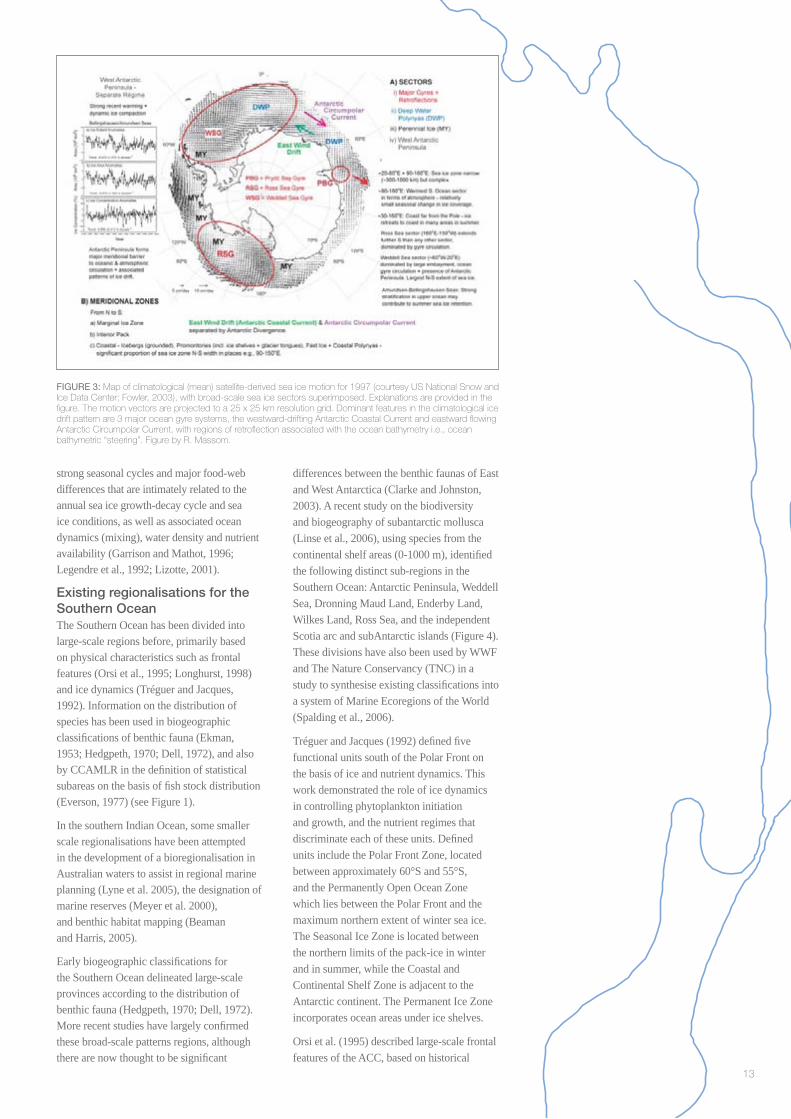
The major features driving the dynamics of sea ice are shown in Figure 3.

The Antarctic Peninsula region is the only Antarctic sector to have experienced a rapid warming trend over the past 50 years, of ~0.5oC per decade (Vaughan et al., 2001). Moreover, the West Antarctic Peninsula (WAP) region is the only Antarctic sector to

have experienced a statistically signifi cant decreasing trend in sea ice areal extent since 1978 (see inset in Figure 3, from Kwok and Comiso, 2002). Recent results imply that this change may result from changes in dynamic (i.e., wind-driven) forcing (Massom et al., 2006). These factors, combined with the profound impact of the Antarctic Peninsula as a meridional blocking feature that extends to low latitudes and oceanic characteristics, suggest that the WAP region should be treated as a separate regime.

Forming an important habitat for a wide range of organisms specifi cally adapted to its presence, sea ice plays a dominant defi ning role in structuring high-latitude marine ecosystems (Ackley and Sullivan, 1994; Brierley and Thomas, 2002; Eicken, 1992; Lizotte and Arrigo, 1998; Nicol and Allison, 1997), and on a variety of scales. The most productive areas of the Southern Ocean lie in the Seasonal Ice Zone, between the maximum northern extents of sea ice in winter and summer. Here in particular, Antarctic krill and other planktonic organisms support an abundance of fi sh, birds, seals and whales. In addition, the ice edge is typically a region of enhanced biological activity during the melt season in particular (Nicol and Allison, 1997; Smith and Nelson, 1986; Smith et al., 1988; Sullivan et al., 1993).

Although in the past characterised as simple, the Antarctic food web involves complex relationships between primary producers and higher predators, as well as abiotic factors. The Antarctic ecosystem is characterised by

13

FIGURE 3: Map of climatological (mean) satellite-derived sea ice motion for 1997 (courtesy US National Snow and Ice Data Center; Fowler, 2003), with broad-scale sea ice sectors superimposed. Explanations are provided in the fi gure. The motion vectors are projected to a 25 x 25 km resolution grid. Dominant features in the climatological ice drift pattern are 3 major ocean gyre systems, the westward-drifting Antarctic Coastal Current and eastward fl owing Antarctic Circumpolar Current, with regions of retrofl ection associated with the ocean bathymetry i.e., ocean bathymetric “steering”. Figure by R. Massom.

strong seasonal cycles and major food-web differences that are intimately related to the annual sea ice growth-decay cycle and sea ice conditions, as well as associated ocean dynamics (mixing), water density and nutrient availability (Garrison and Mathot, 1996; Legendre et al., 1992; Lizotte, 2001).

Existing regionalisations for the Southern OceanThe Southern Ocean has been divided into large-scale regions before, primarily based on physical characteristics such as frontal features (Orsi et al., 1995; Longhurst, 1998) and ice dynamics (Tréguer and Jacques, 1992). Information on the distribution of species has been used in biogeographic classifi cations of benthic fauna (Ekman, 1953; Hedgpeth, 1970; Dell, 1972), and also by CCAMLR in the defi nition of statistical subareas on the basis of fi sh stock distribution (Everson, 1977) (see Figure 1).

In the southern Indian Ocean, some smaller scale regionalisations have been attempted in the development of a bioregionalisation in Australian waters to assist in regional marine planning (Lyne et al. 2005), the designation of marine reserves (Meyer et al. 2000), and benthic habitat mapping (Beaman and Harris, 2005).

Early biogeographic classifi cations for the Southern Ocean delineated large-scale provinces according to the distribution of benthic fauna (Hedgpeth, 1970; Dell, 1972). More recent studies have largely confi rmed these broad-scale patterns regions, although there are now thought to be signifi cant

differences between the benthic faunas of East and West Antarctica (Clarke and Johnston, 2003). A recent study on the biodiversity and biogeography of subantarctic mollusca (Linse et al., 2006), using species from the continental shelf areas (0-1000 m), identifi ed the following distinct sub-regions in the Southern Ocean: Antarctic Peninsula, Weddell Sea, Dronning Maud Land, Enderby Land, Wilkes Land, Ross Sea, and the independent Scotia arc and subAntarctic islands (Figure 4). These divisions have also been used by WWF and The Nature Conservancy (TNC) in a study to synthesise existing classifi cations into a system of Marine Ecoregions of the World (Spalding et al., 2006).

Tréguer and Jacques (1992) defi ned fi ve functional units south of the Polar Front on the basis of ice and nutrient dynamics. This work demonstrated the role of ice dynamics in controlling phytoplankton initiation and growth, and the nutrient regimes that discriminate each of these units. Defi ned units include the Polar Front Zone, located between approximately 60°S and 55°S, and the Permanently Open Ocean Zone which lies between the Polar Front and the maximum northern extent of winter sea ice. The Seasonal Ice Zone is located between the northern limits of the pack-ice in winter and in summer, while the Coastal and Continental Shelf Zone is adjacent to the Antarctic continent. The Permanent Ice Zone incorporates ocean areas under ice shelves.

Orsi et al. (1995) described large-scale frontal features of the ACC, based on historical

14

FIGURE 6: Classifi cation of the Southern Ocean, Longhurst (1998) (Reprinted from: Ecological Geography of the Sea, A.R. Longhurst. Copyright (1998), with permission from Elsevier)

FIGURE 5: Fronts of the Southern Ocean, as defi ned by Orsi et al. (1995)

0 1000 2000500 Km

Projection: Polar stereographicTrue scale at 71∞S

30∞W

150∞W 180∞

0∞

150∞E

30∞E

40∞S 40∞S

40∞S 40∞S

90∞W 90∞E

sACC boundarysACC

STF

SAF

PF

hydrographic data. Gradients in ocean surface properties were used to defi ne three major fronts within the ACC which separate water masses and fl ow characteristics. These are shown in Figure 5.

Longhurst (1998) proposed a global system of ocean classifi cation based on a simple set of environmental variables (sea surface temperature, mixed layer depth, nutrient dynamics and circulation) together with planktonic algal ecology. In this classifi cation scheme (Figure 6) the Southern Ocean includes two provinces in the Westerly Winds Biome between approximately 40oS and 50oS (South Subtropical Convergence Province and SubAntarctic Water Ring Province) and two in the Antarctic Polar Biome between 50oS and the continental coast (Antarctic Province and Austral Polar Province).

The LME classifi cation system defi nes the Southern Ocean as a single unit (Sherman and Duda, 1999), while several other classifi cations defi ne only a small number of concentric rings around the continent. However, the Southern Ocean has a variety of distinct provinces within these larger regions which differ in their chemical, physical and ecological characteristics, and which show considerable longitudinal, as well as latitudinal variation. Improved data coverage and availability through satellite imaging, and improved understanding of ocean characteristics through ecosystem modelling makes it now possible to elaborate on these previous regionalisations using a wider range and broader coverage of data.

FIGURE 4: Biogeographic areas of the Southern Ocean defi ned by Linse et al. (2006), using distribution records for shelf (0-1000 m) species of shelled gastropods and bivalves(Figure reprinted with permission from: Linse et al, 2006)

15

1.4 Experts Workshop

The aim of the Experts Workshop was to review the methods for identifying major provinces, collate available synoptic datasets, and to gain input and recommendations from experts on the process and the results. In particular, the workshop aimed to develop a “proof of concept” for a broad-scale bioregionalisation of the Southern Ocean, using physical and environmental data as the primary input.

A list of the workshop participants is provided at the end of this report.

Specifi c objectives of the workshop were to:• review and assess the processes developed to date and the proposed methods;• discuss and make recommendations on data types to be included in a broad-scale bioregionalisation;• collate appropriate datasets;• apply the approved method(s) to the Southern Ocean using available datasets, to test and validate the process and produce a ‘proof of concept’ including maps of the defi ned broad-scale provinces;• assess preliminary results and broad-scale provinces, given present knowledge of the Southern Ocean.• provide recommendations on products to be developed, including the fi nal report, maps, illustrations, datasets and a GIS (or other) database; and• provide recommendations on datasets and/or method(s) that might be used to develop further fi ne-scale bioregionalisations.

The workshop was held over fi ve days, and included background presentations, plenary discussion, and computer-based analysis in small groups.

At the start of the workshop, background presentations were given on some of the major physical processes in the Southern Ocean, and initial discussion focused on the relationships between physical and ecological processes. A series of presentations were also given on approaches to bioregionalisation that have been undertaken elsewhere, which allowed detailed consideration of the application of different methods.

Participants then investigated different aspects of data analysis and refi nement of methods in small groups, focusing initially on their regions of particular expertise (e.g. South Atlantic, East Antarctica, Ross Sea) and later looking at the Southern Ocean as a whole. Selected physical datasets were provided for use in the initial analysis, and others were made available by participants during the week. The analytical methods used by Lyne and Hayes (2005), Leathwick et al. (2006a) and Raymond and Constable (2006) were used as starting points for the analysis during the workshop. These methods were refi ned into a single methodology, following workshop discussions and practical explorations of the methods. Appendix I gives further details on the background and technical aspects of each of these methods.

The fi nal stages of the workshop included discussion on how well the defi ned regions corresponded to our present knowledge of the Southern Ocean. Priorities were identifi ed for further work on issues including uncertainty, understanding of inter- and intra-annual variation, validation of results, the use of additional data (particularly biological datasets) and fi ner-scale analysis of particular areas of interest.

The Southern Ocean covers around 10% of the world’s ocean surface, and includes some of the most productive marine regions on Earth. Although they are among the least-studied, the seas around Antarctica are a critical component of the global climate system and marine ecosystem.

16

2. Approach to bioregionalisation

This section describes the approach to bioregionalisation that was used as a starting point for the workshop discussions and analysis. Descriptions of each step are presented here, together with background information on issues that must be considered. Further technical detail is provided in Appendix II. A summary of the fi nal method adopted is presented in Section 3.

The regionalisation process can be partitioned into the following steps:

1. Identify the ecological patterns and processes that have relevance to the end- use application of the regionalisation

2. Identify the major environmental drivers or properties that control these patterns and processes, and extract relevant parameters describing those properties

3. Pre-process the data (e.g. normalise, transform, smooth)

4. Compile a data matrix of individual sites (rows) by properties (columns)

5. Apply a clustering procedure to group sites with similar properties

6. Post-process the clusters to meet any application-specifi c constraints on the regions (e.g. minimum size)

7. Expert review of the regions to ensure suitability for the application.

This process can be iterative. Ideally, the initial process will establish the mechanisms by which new data and/or knowledge could be incorporated into revisions of the bioregionalisation, although this would be expected to assist more in establishing or revising smaller scale subdivisions rather than altering the higher level bioregionalisation.

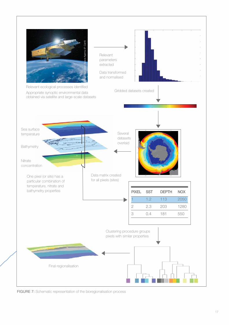
Figure 7 is a schematic representation of the bioregionalisation process, illustrating how data selected to refl ect ecological processes can be used to defi ne bioregions.

© W

WF-

Can

on, S

ylvi

a R

UB

LI

17

FIGURE 7: Schematic representation of the bioregionalisation process

PIXEL SST DEPTH NOX

1 1.2 113 2050

2 2.3 203 1280

3 0.4 181 550

Final regionalisation

One pixel (or site) has a particular combination of temperature, nitrate and bathymetry properties

Relevant ecological processes identifi ed

Appropriate synoptic environmental data obtained via satellite and large-scale datasets

Clustering procedure groups pixels with similar properties

Data matrix created for all pixels (sites)

Several datasets overlaid

Gridded datasets created

Relevant parameters extracted

Data transformed and normalised

0 1000 2000500 Km

Projection: Polar stereographicTrue scale at 71∞S

30∞W

150∞W 180∞

0∞

150∞E

30∞E

40∞S 40∞S

40∞S 40∞S

90∞W 90∞E

Sea surface temperature

Bathymetry

Nitrate concentration

Imag

e: E

urop

ean

Spa

ce A

genc

y (P

. Car

ril)

18

An important fi rst step in the bioregionalisation analysis is to identify distinct ecological processes and their defi ning properties. The identifi cation of ecological processes to be captured in the regionalisation is likely to be driven by the requirements of a particular end-use application.

Ideally, a bioregionalisation would delineate units that, depending on the scale, clearly separate habitats, communities and ecosystems. In this ideal world, populations would reside wholly within these areas.In reality, there is considerable complexity that needs to be addressed because of the different relationships that species have with the environment and other biota (Andrewartha & Birch 1984). A bioregionalisation aims to capture the properties of the important relationships rather than, necessarily, simply trying to circumscribe the distributions of whole populations of species.

This concept is illustrated in Figure 8. Some species will be found closely aligned with environmental gradients. Other species will appear in areas with high levels of perturbation, such that environmental factors are mixed and ever changing in their relative distributions. Yet others will exploit the diversity of patches in fringing habitats and ecotones. For mobile species, some taxa will be found across most areas but only some areas will be important to them as feeding or reproductive areas. An important step in the process is to determine how to accommodate environmental gradients and overlaps in the regionalisation.

The marine environment comprises three dimensions – geographic space and depth. Distribution of biota in the pelagic environment is mostly determined by the potential productivity in the water masses and the movement of those water masses in space and depth. The benthic environment has additional features refl ecting variation in the depth, substratum types and roughness of the seafl oor, and the degree to which this promotes interaction with the pelagic realm. These features are often considered to the primary drivers of environmental heterogeneity. Secondary drivers are more ephemeral or changing over time. In the Antarctic, they would also include other features of the environment such as the annual cycle of advance and retreat of the sea ice zone.

A bioregionalisation would generally try to represent the heterogeneity in ecosystem

structure and function, which primarily would subdivide areas according to the magnitude of productivity and its predictability in time. Further subdivision would relate to the diversity of habitats and the relationships of species and food-webs to those habitats. The process will need to differentiate between areas with relatively constant features from those that are highly variable, even though they may have similar mean values. This is because a region with a large amount of disturbance can accommodate different assemblages involving opportunistic species as well as those that require long-term stability. Some areas in a bioregionalisation may need to represent large areas of habitat discontinuity or disturbance, which could be important regions in themselves. As a result of these considerations, a goal for a bioregionalisation is to capture not only the differences in diversity and the suite of ecosystem relationships, but also the potential differences in environmental stability.

2.1 Identifying properties to be captured

FIGURE 8: Conceptual diagram illustrating potential relationships between species along gradients of environmental parameters.

FIGURE 8(a): distribution of species with respect to a single environmental gradient, say temperature. Each polygon represents a different taxon, colours represent similar taxa. Width of bars represents relative abundance for a taxon.

FIGURE 8(b): as for (a) but with distributions relative to two environmental gradients - distributions on gradient 1 are as in (a). A general discontinuity between species distributions in (a) might be roughly at the midpoint (green on the environmental gradient). In (b) the separation between groups of taxa becomes clearer on the second gradient.

LONGITUDE

LATITUDE

ENVI

RO

NM

ENTA

L G

RA

DIE

NT

2

ENVIRONMENTAL GRADIENT 1

ENVIRONMENTAL GRADIENT 1

FIGURE 8(c): The environmental conditions form a patchwork in geographic space which can result in regions of similar environmental conditions being separated geographically. Here, parallelograms represent spatial areas with colours representing two environmental parameters (outer colour is from environmental gradient 1 and inner colour is from gradient 2). Each area is expected to have a species composition consistent with that composition at the intersection of two respective environmental gradient colours in (b).

19

The intent of a regionalisation is to partition the study area into a set of discrete spatial regions, each with relatively homogeneous ecosystem properties. In the bioregionalisation analysis, regions are selected by grouping sites with particular characteristics. In some cases there may be specifi c, known characteristics that can be used to delineate region boundaries, such as water temperature changes across oceanic fronts. Another example is to separate the continental shelf from the continental slope by choosing an appropriate bathymetric contour, say 1000 m. Generally, however, the expectation is that the regions will refl ect a natural clustering of the environmental or biotic data.

Clustering algorithms are well suited to bioregionalisation analysis, as they are designed to partition a large data set into a number of subsets, each with relatively similar properties that differ from those of the other subsets. In the context of a regionalisation, the clustering process takes sites (or cells) from a grid in geographic space. Each site has associated ecological properties (physical and/or biotic data) and this information is used to group together sites with relatively similar ecological properties.

Those groupings (which are calculated in ‘environmental space’, i.e. based only on environmental properties, and ignoring spatial information) are then projected back into geographic space in order to fi nd the spatial extents of the resulting regions. Thus, the regions are discrete in environmental space, but may be scattered or fragmented in geographical space (i.e. there may be several regions with the same properties located in different geographic areas).

Choosing clustering algorithmsThere are a large number of clustering algorithms that could potentially be used, all of which have assumptions or limitations that may preclude their use in particular circumstances or with particular types of data. Thus, the outcomes of the bioregionalisation could be infl uenced by the choice of the algorithm. The aim is to develop a clustering process that is consistent with the data and for which the results are likely not to change much with alternative clustering algorithms. Consideration will need to be given, inter alia, to algorithm assumptions, complexity, and accuracy.

It is important to make the distinction between the clusters that are produced by a clustering algorithm, and the regions that

are formed from those clusters. A cluster is a group of sites that are considered to have similar environmental properties. However, because the clustering process is based on environmental similarity (and not spatial information), a single cluster may contain sites that are spatially separated. A region is thus considered to be a group of sites that belong to the same cluster, but which also form a contiguous spatial area. A single cluster may produce a number of regions, each of which have the same general properties, but which are spatially distinct.

Clustering algorithms are often based around the concept of a dissimilarity metric, which (in the context of a regionalisation) is used to calculate how dissimilar two sites are, given their ecosystem properties (physical or biological data). The clustering of sites into regions is carried out in such a way that the intra-region dissimilarity of sites is low (i.e. sites within a region are similar to each other) relative to inter-region dissimilarities. Dissimilarity-based clustering methods can be broadly divided into hierarchical or non-hierarchical schemes. Further information on these schemes, and the issues related to selecting clustering algorithms, is provided in Appendix II.

2.2 Classifi cation method

Pho

togr

aph

by B

rian

Bal

l, A

ustr

alia

n G

over

nmen

t Ant

arct

ic D

ivis

ion

© C

omm

onw

ealth

of A

ustr

alia

20

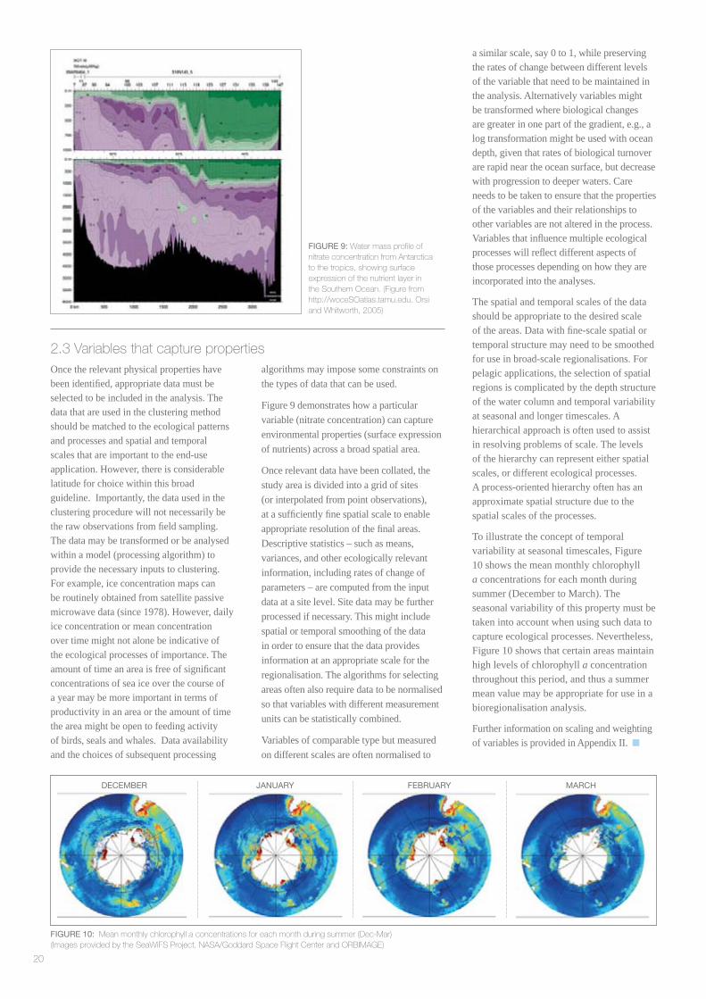
2.3 Variables that capture propertiesOnce the relevant physical properties have been identifi ed, appropriate data must be selected to be included in the analysis. The data that are used in the clustering method should be matched to the ecological patterns and processes and spatial and temporal scales that are important to the end-use application. However, there is considerable latitude for choice within this broad guideline. Importantly, the data used in the clustering procedure will not necessarily be the raw observations from fi eld sampling. The data may be transformed or be analysed within a model (processing algorithm) to provide the necessary inputs to clustering. For example, ice concentration maps can be routinely obtained from satellite passive microwave data (since 1978). However, daily ice concentration or mean concentration over time might not alone be indicative of the ecological processes of importance. The amount of time an area is free of signifi cant concentrations of sea ice over the course of a year may be more important in terms of productivity in an area or the amount of time the area might be open to feeding activity of birds, seals and whales. Data availability and the choices of subsequent processing

algorithms may impose some constraints on the types of data that can be used.

Figure 9 demonstrates how a particular variable (nitrate concentration) can capture environmental properties (surface expression of nutrients) across a broad spatial area.

Once relevant data have been collated, the study area is divided into a grid of sites (or interpolated from point observations), at a suffi ciently fi ne spatial scale to enable appropriate resolution of the fi nal areas. Descriptive statistics – such as means, variances, and other ecologically relevant information, including rates of change of parameters – are computed from the input data at a site level. Site data may be further processed if necessary. This might include spatial or temporal smoothing of the data in order to ensure that the data provides information at an appropriate scale for the regionalisation. The algorithms for selecting areas often also require data to be normalised so that variables with different measurement units can be statistically combined.

Variables of comparable type but measured on different scales are often normalised to

FIGURE 9: Water mass profi le of nitrate concentration from Antarctica to the tropics, showing surface expression of the nutrient layer in the Southern Ocean. (Figure from http://woceSOatlas.tamu.edu. Orsi and Whitworth, 2005)

FIGURE 10: Mean monthly chlorophyll a concentrations for each month during summer (Dec-Mar)(Images provided by the SeaWiFS Project, NASA/Goddard Space Flight Center and ORBIMAGE)

a similar scale, say 0 to 1, while preserving the rates of change between different levels of the variable that need to be maintained in the analysis. Alternatively variables might be transformed where biological changes are greater in one part of the gradient, e.g., a log transformation might be used with ocean depth, given that rates of biological turnover are rapid near the ocean surface, but decrease with progression to deeper waters. Care needs to be taken to ensure that the properties of the variables and their relationships to other variables are not altered in the process. Variables that infl uence multiple ecological processes will refl ect different aspects of those processes depending on how they are incorporated into the analyses.

The spatial and temporal scales of the data should be appropriate to the desired scale of the areas. Data with fi ne-scale spatial or temporal structure may need to be smoothed for use in broad-scale regionalisations. For pelagic applications, the selection of spatial regions is complicated by the depth structure of the water column and temporal variability at seasonal and longer timescales. A hierarchical approach is often used to assist in resolving problems of scale. The levels of the hierarchy can represent either spatial scales, or different ecological processes. A process-oriented hierarchy often has an approximate spatial structure due to the spatial scales of the processes.

To illustrate the concept of temporal variability at seasonal timescales, Figure 10 shows the mean monthly chlorophyll a concentrations for each month during summer (December to March). The seasonal variability of this property must be taken into account when using such data to capture ecological processes. Nevertheless, Figure 10 shows that certain areas maintain high levels of chlorophyll a concentration throughout this period, and thus a summer mean value may be appropriate for use in a bioregionalisation analysis.

Further information on scaling and weighting of variables is provided in Appendix II.

DECEMBER JANUARY FEBRUARY MARCH

21

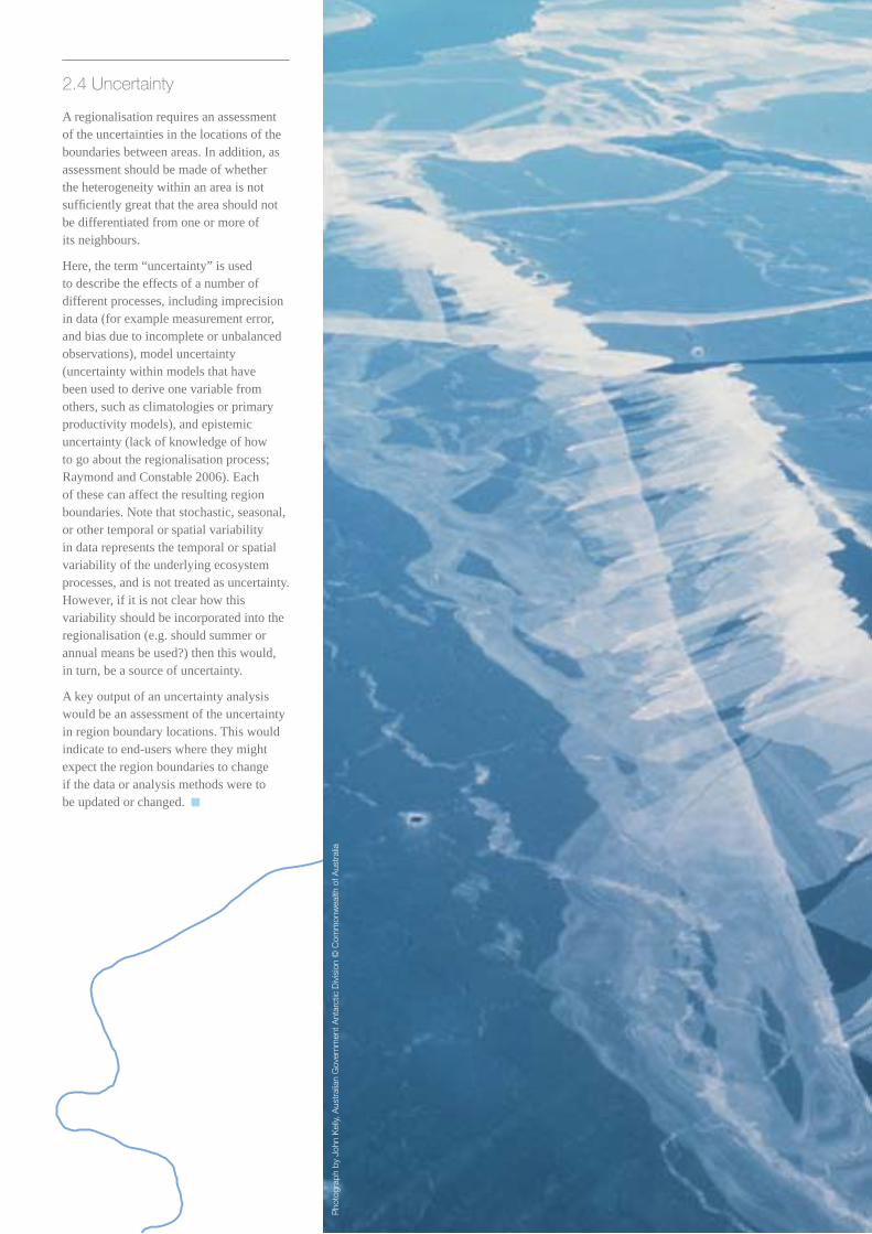
A regionalisation requires an assessment of the uncertainties in the locations of the boundaries between areas. In addition, as assessment should be made of whether the heterogeneity within an area is not suffi ciently great that the area should not be differentiated from one or more of its neighbours.

Here, the term “uncertainty” is used to describe the effects of a number of different processes, including imprecision in data (for example measurement error, and bias due to incomplete or unbalanced observations), model uncertainty (uncertainty within models that have been used to derive one variable from others, such as climatologies or primary productivity models), and epistemic uncertainty (lack of knowledge of how to go about the regionalisation process; Raymond and Constable 2006). Each of these can affect the resulting region boundaries. Note that stochastic, seasonal, or other temporal or spatial variability in data represents the temporal or spatial variability of the underlying ecosystem processes, and is not treated as uncertainty. However, if it is not clear how this variability should be incorporated into the regionalisation (e.g. should summer or annual means be used?) then this would, in turn, be a source of uncertainty.

A key output of an uncertainty analysis would be an assessment of the uncertainty in region boundary locations. This would indicate to end-users where they might expect the region boundaries to change if the data or analysis methods were to be updated or changed.

2.4 Uncertainty

Pho

togr

aph

by J

ohn

Kel

ly, A

ustr

alia

n G

over

nmen

t Ant

arct

ic D

ivis

ion

© C

omm

onw

ealth

of A

ustr

alia

22

Pho

togr

aph

by G

rant

Dix

on, A

ustr

alia

n G

over

nmen

t Ant

arct

ic D

ivis

ion

© C

omm

onw

ealth

of A

ustr

alia

23

3. Physical regionalisation

3.1 Summary of adopted method

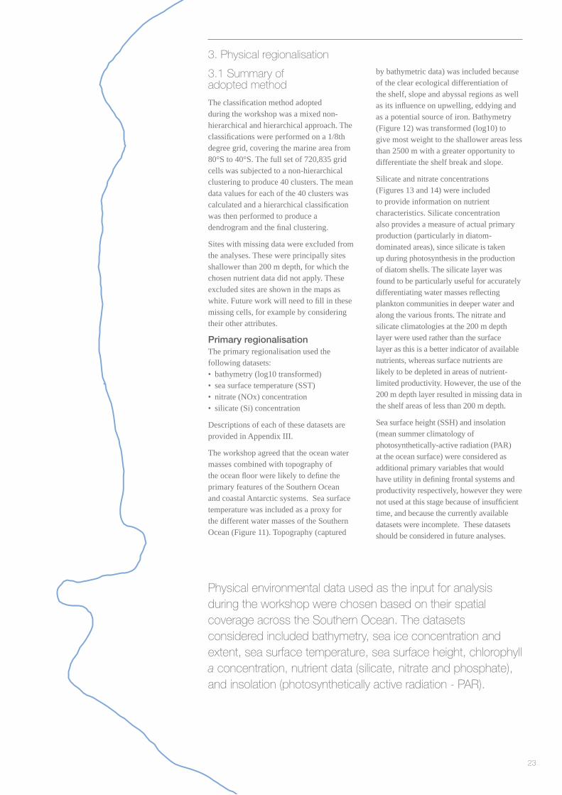
The classifi cation method adopted during the workshop was a mixed non-hierarchical and hierarchical approach. The classifi cations were performed on a 1/8th degree grid, covering the marine area from 80°S to 40°S. The full set of 720,835 grid cells was subjected to a non-hierarchical clustering to produce 40 clusters. The mean data values for each of the 40 clusters was calculated and a hierarchical classifi cation was then performed to produce a dendrogram and the fi nal clustering.

Sites with missing data were excluded from the analyses. These were principally sites shallower than 200 m depth, for which the chosen nutrient data did not apply. These excluded sites are shown in the maps as white. Future work will need to fi ll in these missing cells, for example by considering their other attributes.

Primary regionalisationThe primary regionalisation used the following datasets:• bathymetry (log10 transformed)• sea surface temperature (SST)• nitrate (NOx) concentration• silicate (Si) concentration

Descriptions of each of these datasets are provided in Appendix III.

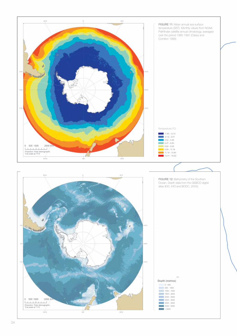
The workshop agreed that the ocean water masses combined with topography of the ocean fl oor were likely to defi ne the primary features of the Southern Ocean and coastal Antarctic systems. Sea surface temperature was included as a proxy for the different water masses of the Southern Ocean (Figure 11). Topography (captured

by bathymetric data) was included because of the clear ecological differentiation of the shelf, slope and abyssal regions as well as its infl uence on upwelling, eddying and as a potential source of iron. Bathymetry (Figure 12) was transformed (log10) to give most weight to the shallower areas less than 2500 m with a greater opportunity to differentiate the shelf break and slope.

Silicate and nitrate concentrations (Figures 13 and 14) were included to provide information on nutrient characteristics. Silicate concentration also provides a measure of actual primary production (particularly in diatom-dominated areas), since silicate is taken up during photosynthesis in the production of diatom shells. The silicate layer was found to be particularly useful for accurately differentiating water masses refl ecting plankton communities in deeper water and along the various fronts. The nitrate and silicate climatologies at the 200 m depth layer were used rather than the surface layer as this is a better indicator of available nutrients, whereas surface nutrients are likely to be depleted in areas of nutrient-limited productivity. However, the use of the 200 m depth layer resulted in missing data in the shelf areas of less than 200 m depth.

Sea surface height (SSH) and insolation (mean summer climatology of photosynthetically-active radiation (PAR) at the ocean surface) were considered as additional primary variables that would have utility in defi ning frontal systems and productivity respectively, however they were not used at this stage because of insuffi cient time, and because the currently available datasets were incomplete. These datasets should be considered in future analyses.

Physical environmental data used as the input for analysis during the workshop were chosen based on their spatial coverage across the Southern Ocean. The datasets considered included bathymetry, sea ice concentration and extent, sea surface temperature, sea surface height, chlorophyll a concentration, nutrient data (silicate, nitrate and phosphate), and insolation (photosynthetically active radiation - PAR).

24

FIGURE 12: Bathymetry of the Southern Ocean. Depth data from the GEBCO digital atlas (IOC, IHO and BODC, 2003).

FIGURE 11: Mean annual sea surface temperature (SST). Monthly values from NOAA Pathfi nder satellite annual climatology, averaged over the period 1985-1997 (Casey and Cornillon 1999)

Depth (metres)

0 - 500

500 - 1000

1000 - 1500

1500 - 2000

2000 - 2500

2500 - 3000

3000 - 4000

4000 - 5000

> 5000

150oW

-1.95 - -0.13

-0.12 - 2.01

2.02 - 4.46

4.47 - 6.83

6.84 - 9.05

9.06 - 11.18

11.19 - 13.40

13.41 - 18.22

Temperature (°C)

25

FIGURE 14: Nitrate concentration (at 200 m depth). Climatology from the WOCE global hydrographic climatology (Gouretski and Koltermann, 2004)

FIGURE 13: Silicate concentration (at 200 m depth). Climatology from the WOCE global hydrographic climatology (Gouretski and Koltermann, 2004)

2.47 - 4.58

4.59 - 7.96

7.97 - 18.08

18.09 - 38.76

38.77 - 64.93

64.94 - 76.74

76.75 - 86.87

86.88 - 110.08

Si (umol/kg)

5.55 - 12.40

12.41 - 15.58

15.59 - 18.65

18.66 - 21.72

21.73 - 25.38

25.39 - 29.27

29.28 - 32.34

32.35 - 35.65

NOx (umol/kg)

26

Secondary regionalisationThe Workshop agreed that the bioregionalisation should ideally differentiate fi rst between the main divisions of coastal Antarctica (shelf and slope areas), sea ice zone and northern open ocean waters before further subdividing according to secondary features. Nevertheless, two potential components of a secondary classifi cation were explored to determine if there is suffi cient spatial heterogeneity to warrant a further subdivision.

Sea ice was considered to modify the pelagic environment both in terms of the potential for primary production as well its infl uence on the distribution of marine mammals and birds. The impact of sea ice on the environment was explored using a data layer comprising the number of days an area was covered by at least 15% concentration of sea ice (Figure 15).

The concentration of satellite-observed sea surface chlorophyll was explored using a data layer comprising log transformed chlorophyll a densities (Figure 16). The chlorophyll distribution was truncated at 10 mg.m-3 (where all values greater than 10 were made equal to 10), because the variability in higher order productivity most likely results from variability in the range from 0-10 mg.m-3. While chlorophyll a concentration may not refl ect primary production absolutely, it was considered to be a suitable proxy for the purposes of exploring spatial heterogeneity in primary production at the large scale.

Descriptions of each of these datasets are provided in Appendix III.

Pho

togr

aphe

r: J

ohn

van

den

Hof

f, A

ustr

alia

n G

over

nmen

t Ant

arct

ic D

ivis

ion,

© C

omm

onw

ealth

of A

ustr

alia

27

FIGURE 16: Mean summer (DEC-FEB) surface chlorophyll-a concentrations. Summer means (1998-2004) from SeaWiFS.

0.06

0.07 - 0.22

0.23 - 0.37

0.38 - 0.53

0.54 - 0.68

0.69 - 0.99

1.00 - 1.77

1.78 - 39.80

Chlorophyll-a concentration (mg.m-3)

FIGURE 15: Proportion (0-1) of the year for which the ocean is covered by at least 15% sea ice. Calculated from satellite-derived estimates of sea ice concentration spanning 1979–2003. (Comiso, 1999

0

0.01 - 0.08

0.09 - 0.31

0.32 - 0.49

0.50 - 0.63

0.64 - 0.76

0.77 - 0.91

0.92 - 1

Proportion (0-1)

28

Pho

togr

aph

by N

ick

Gal

es, A

ustr

alia

n G

over

nmen

t Ant

arct

ic D

ivis

ion

© C

omm

onw

ealth

of A

ustr

alia

29

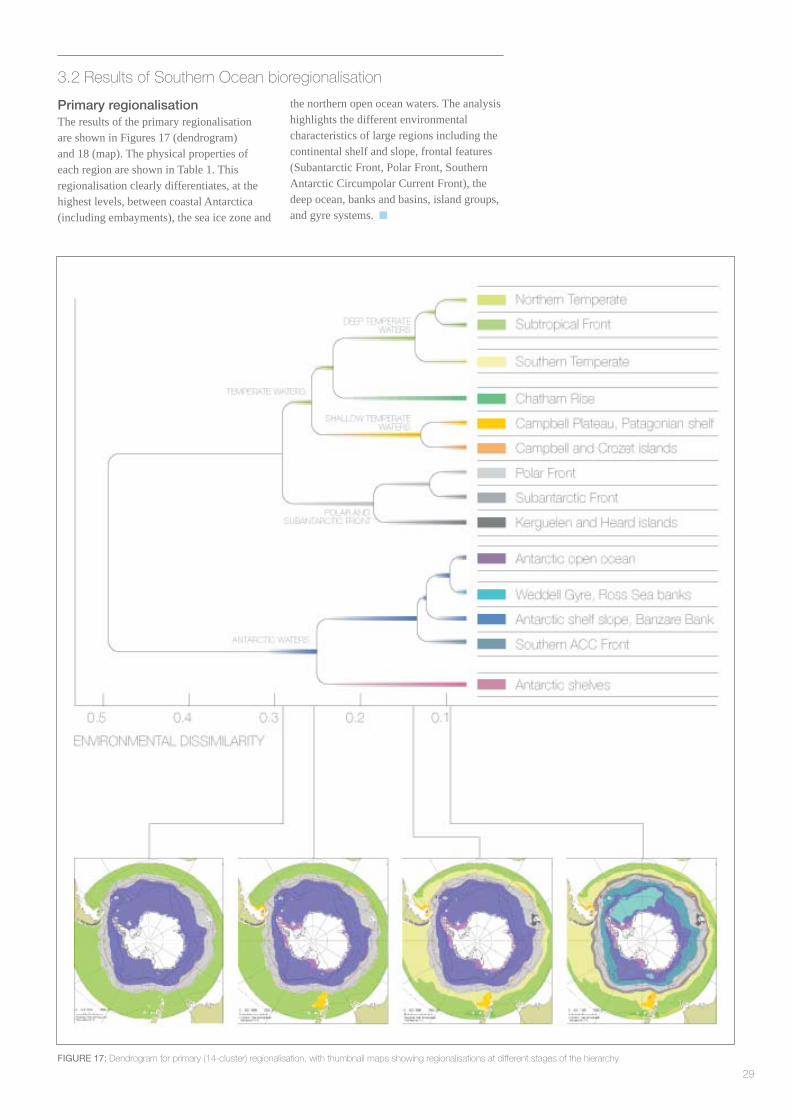
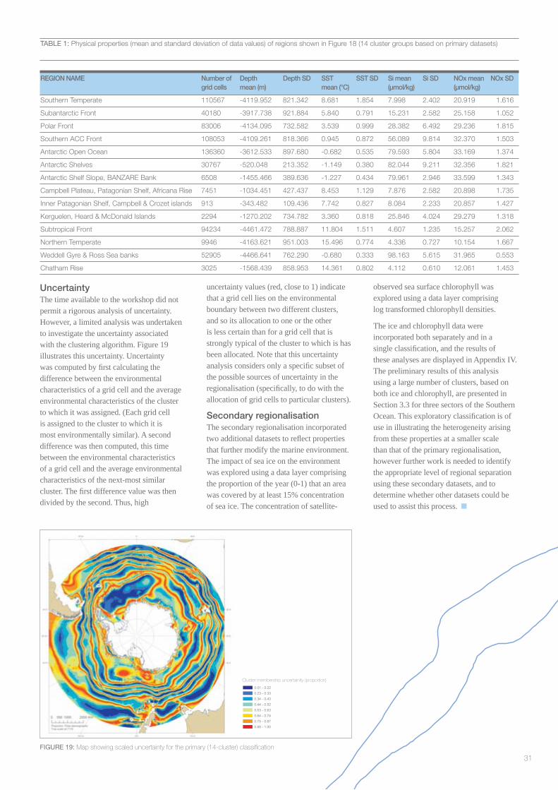
3.2 Results of Southern Ocean bioregionalisation

Primary regionalisationThe results of the primary regionalisation are shown in Figures 17 (dendrogram) and 18 (map). The physical properties of each region are shown in Table 1. This regionalisation clearly differentiates, at the highest levels, between coastal Antarctica (including embayments), the sea ice zone and

the northern open ocean waters. The analysis highlights the different environmental characteristics of large regions including the continental shelf and slope, frontal features (Subantarctic Front, Polar Front, Southern Antarctic Circumpolar Current Front), the deep ocean, banks and basins, island groups, and gyre systems.

FIGURE 17: Dendrogram for primary (14-cluster) regionalisation, with thumbnail maps showing regionalisations at different stages of the hierarchy

30

FIGURE 18: Primary regionalisation of the Southern Ocean based on: depth, sea surface temperature (SST), silicate (Si) and nitrate (NOx) concentrations (14 cluster groups) (white areas represent cells with missing data that were not classifi ed in these analyses).

31

UncertaintyThe time available to the workshop did not permit a rigorous analysis of uncertainty. However, a limited analysis was undertaken to investigate the uncertainty associated with the clustering algorithm. Figure 19 illustrates this uncertainty. Uncertainty was computed by fi rst calculating the difference between the environmental characteristics of a grid cell and the average environmental characteristics of the cluster to which it was assigned. (Each grid cell is assigned to the cluster to which it is most environmentally similar). A second difference was then computed, this time between the environmental characteristics of a grid cell and the average environmental characteristics of the next-most similar cluster. The fi rst difference value was then divided by the second. Thus, high

uncertainty values (red, close to 1) indicate that a grid cell lies on the environmental boundary between two different clusters, and so its allocation to one or the other is less certain than for a grid cell that is strongly typical of the cluster to which is has been allocated. Note that this uncertainty analysis considers only a specifi c subset of the possible sources of uncertainty in the regionalisation (specifi cally, to do with the allocation of grid cells to particular clusters).

Secondary regionalisationThe secondary regionalisation incorporated two additional datasets to refl ect properties that further modify the marine environment. The impact of sea ice on the environment was explored using a data layer comprising the proportion of the year (0-1) that an area was covered by at least 15% concentration of sea ice. The concentration of satellite-

observed sea surface chlorophyll was explored using a data layer comprising log transformed chlorophyll densities.

The ice and chlorophyll data were incorporated both separately and in a single classifi cation, and the results of these analyses are displayed in Appendix IV. The preliminary results of this analysis using a large number of clusters, based on both ice and chlorophyll, are presented in Section 3.3 for three sectors of the Southern Ocean. This exploratory classifi cation is of use in illustrating the heterogeneity arising from these properties at a smaller scale than that of the primary regionalisation, however further work is needed to identify the appropriate level of regional separation using these secondary datasets, and to determine whether other datasets could be used to assist this process.

FIGURE 19: Map showing scaled uncertainty for the primary (14-cluster) classifi cation

TABLE 1: Physical properties (mean and standard deviation of data values) of regions shown in Figure 18 (14 cluster groups based on primary datasets)

REGION NAME Number of Depth Depth SD SST SST SD Si mean Si SD NOx mean NOx SD grid cells mean (m) mean (°C) (µmol/kg) (µmol/kg)

Southern Temperate 110567 -4119.952 821.342 8.681 1.854 7.998 2.402 20.919 1.616

Subantarctic Front 40180 -3917.738 921.884 5.840 0.791 15.231 2.582 25.158 1.052

Polar Front 83006 -4134.095 732.582 3.539 0.999 28.382 6.492 29.236 1.815

Southern ACC Front 108053 -4109.261 818.366 0.945 0.872 56.089 9.814 32.370 1.503

Antarctic Open Ocean 136360 -3612.533 897.680 -0.682 0.535 79.593 5.804 33.169 1.374

Antarctic Shelves 30767 -520.048 213.352 -1.149 0.380 82.044 9.211 32.356 1.821

Antarctic Shelf Slope, BANZARE Bank 6508 -1455.466 389.636 -1.227 0.434 79.961 2.946 33.599 1.343

Campbell Plateau, Patagonian Shelf, Africana Rise 7451 -1034.451 427.437 8.453 1.129 7.876 2.582 20.898 1.735

Inner Patagonian Shelf, Campbell & Crozet islands 913 -343.482 109.436 7.742 0.827 8.084 2.233 20.857 1.427

Kerguelen, Heard & McDonald Islands 2294 -1270.202 734.782 3.360 0.818 25.846 4.024 29.279 1.318

Subtropical Front 94234 -4461.472 788.887 11.804 1.511 4.607 1.235 15.257 2.062

Northern Temperate 9946 -4163.621 951.003 15.496 0.774 4.336 0.727 10.154 1.667

Weddell Gyre & Ross Sea banks 52905 -4466.641 762.290 -0.680 0.333 98.163 5.615 31.965 0.553

Chatham Rise 3025 -1568.439 858.953 14.361 0.802 4.112 0.610 12.061 1.453

0.01 - 0.22

0.23 - 0.33

0.34 - 0.43

0.44 - 0.52

0.53 - 0.63

0.64 - 0.74

0.75 - 0.87

0.88 - 1.00

Cluster membership uncertainity (proportion)

32

An assessment of the fi nal results was carried out by expert review to determine if the defi ned regions were consistent with present knowledge of the ecosystem. The following sections describe the defi ned regions in further detail, focusing separately on the Atlantic, Indian and Pacifi c ocean sectors (CCAMLR Statistical Areas 48, 58 and 88, respectively). For each sector, a map of the regions defi ned by the primary regionalisation is overlain with information on known large-scale physical and ecological features such as fronts, gyres, seamounts and maximum sea ice extent. In addition, maps showing an example of a secondary regionalisation (using ice and chlorophyll data to defi ne 40 clusters for the Southern Ocean) illustrate the high degree of smaller-scale heterogeneity arising from patchiness in chlorophyll and sea ice concentrations, particularly in shelf areas and the seasonal ice zone.

South Atlantic (Area 48)The Atlantic sector is characterised by the narrowing of the ACC as it passes through Drake Passage between South America and the Antarctic Peninsula. In the west, strong

currents, eddies and mixing associated with the ACC and the Weddell-Scotia Confl uence (WSC) occur in the vicinity of the Scotia Arc. In the central and eastern areas, there is a greater contribution of the Weddell gyre and a broadening of the ACC. A large continental shelf area is present in the great embayment of the Weddell Sea, along with a number of ice shelves. These features are captured well in the primary regionalisation. The Atlantic sector is also dominated by strong seasonal cycles, manifest by changing irradiance and seasonal sea-ice cover. The bathymetry of the southwest Atlantic steers the fl ow of the ACC northwards, carrying polar waters to more northerly latitudes than elsewhere in the Southern Ocean. This transport is critical to the local marine systems around some of the more northerly SubAntarctic island groups where large colonies of many land-based predators breed.

The southwest Atlantic is possibly the most studied of all the areas in the Southern Ocean. It has higher productivity than other areas. Extensive summer phytoplankton blooms, particularly around some of the

island chains, probably result from the mixing of micronutrients with surface waters through the fl ow of the ACC and the WSC as they pass over the Scotia Arc. A range of zooplankton species including Antarctic krill (Euphausia superba), consume this primary production. In turn, these taxa are consumed by numerous species of nekton, seabirds and marine mammals. The resulting biodiversity is possibly higher than elsewhere in the Southern Ocean.

Zooplankton community structure in the southwest Atlantic appears to be dependent upon the timing of the seasonal sea-ice retreat (Ward et al., 2003). Sea-ice infl uences the timing of reproduction; a late retreat delays reproduction and reduces population sizes of a number of zooplankton species. During years of normal sea-ice retreat copepods are more advanced, and there are also higher abundances of krill larvae. This implies that the seasonal environment critically infl uences the biogeography of zooplankton communities in the southwest Atlantic. As a consequence, multi-year datasets that encompass years of differing environmental

3.3 Expert review of bioregionalisation results

FIGURE 20: Map showing primary regionalisation for the South Atlantic sector (Area 48), with major physical features

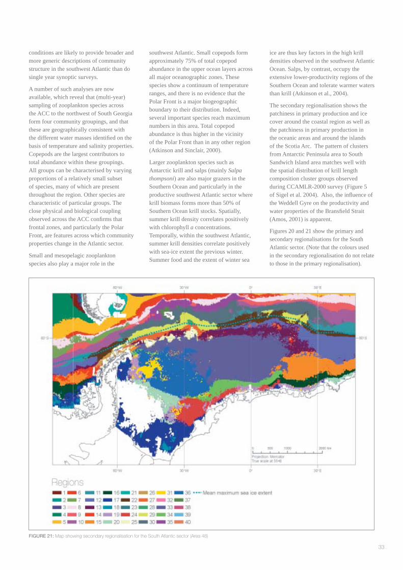
33

conditions are likely to provide broader and more generic descriptions of community structure in the southwest Atlantic than do single year synoptic surveys.

A number of such analyses are now available, which reveal that (multi-year) sampling of zooplankton species across the ACC to the northwest of South Georgia form four community groupings, and that these are geographically consistent with the different water masses identifi ed on the basis of temperature and salinity properties. Copepods are the largest contributors to total abundance within these groupings. All groups can be characterised by varying proportions of a relatively small subset of species, many of which are present throughout the region. Other species are characteristic of particular groups. The close physical and biological coupling observed across the ACC confi rms that frontal zones, and particularly the Polar Front, are features across which community properties change in the Atlantic sector.

Small and mesopelagic zooplankton species also play a major role in the

southwest Atlantic. Small copepods form approximately 75% of total copepod abundance in the upper ocean layers across all major oceanographic zones. These species show a continuum of temperature ranges, and there is no evidence that the Polar Front is a major biogeographic boundary to their distribution. Indeed, several important species reach maximum numbers in this area. Total copepod abundance is thus higher in the vicinity of the Polar Front than in any other region (Atkinson and Sinclair, 2000).

Larger zooplankton species such as Antarctic krill and salps (mainly Salpa thompsoni) are also major grazers in the Southern Ocean and particularly in the productive southwest Atlantic sector where krill biomass forms more than 50% of Southern Ocean krill stocks. Spatially, summer krill density correlates positively with chlorophyll a concentrations. Temporally, within the southwest Atlantic, summer krill densities correlate positively with sea-ice extent the previous winter. Summer food and the extent of winter sea

ice are thus key factors in the high krill densities observed in the southwest Atlantic Ocean. Salps, by contrast, occupy the extensive lower-productivity regions of the Southern Ocean and tolerate warmer waters than krill (Atkinson et al., 2004).

The secondary regionalisation shows the patchiness in primary production and ice cover around the coastal region as well as the patchiness in primary production in the oceanic areas and around the islands of the Scotia Arc. The pattern of clusters from Antarctic Peninsula area to South Sandwich Island area matches well with the spatial distribution of krill length composition cluster groups observed during CCAMLR-2000 survey (Figure 5 of Sigel et al. 2004). Also, the infl uence of the Weddell Gyre on the productivity and water properties of the Bransfi eld Strait (Amos, 2001) is apparent.

Figures 20 and 21 show the primary and secondary regionalisations for the South Atlantic sector. (Note that the colours used in the secondary regionalisation do not relate to those in the primary regionalisation).

FIGURE 21: Map showing secondary regionalisation for the South Atlantic sector (Area 48)

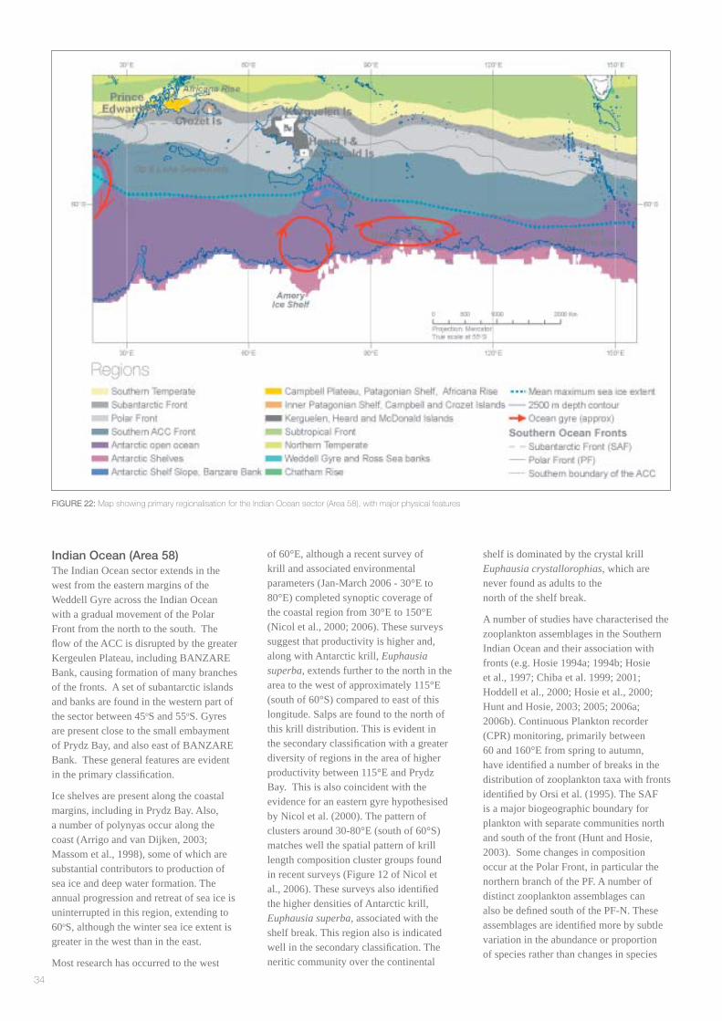
34

FIGURE 22: Map showing primary regionalisation for the Indian Ocean sector (Area 58), with major physical features

Indian Ocean (Area 58)The Indian Ocean sector extends in the west from the eastern margins of the Weddell Gyre across the Indian Ocean with a gradual movement of the Polar Front from the north to the south. The fl ow of the ACC is disrupted by the greater Kergeulen Plateau, including BANZARE Bank, causing formation of many branches of the fronts. A set of subantarctic islands and banks are found in the western part of the sector between 45oS and 55oS. Gyres are present close to the small embayment of Prydz Bay, and also east of BANZARE Bank. These general features are evident in the primary classifi cation.

Ice shelves are present along the coastal margins, including in Prydz Bay. Also, a number of polynyas occur along the coast (Arrigo and van Dijken, 2003; Massom et al., 1998), some of which are substantial contributors to production of sea ice and deep water formation. The annual progression and retreat of sea ice is uninterrupted in this region, extending to 60oS, although the winter sea ice extent is greater in the west than in the east.

Most research has occurred to the west

of 60°E, although a recent survey of krill and associated environmental parameters (Jan-March 2006 - 30°E to 80°E) completed synoptic coverage of the coastal region from 30°E to 150°E (Nicol et al., 2000; 2006). These surveys suggest that productivity is higher and, along with Antarctic krill, Euphausia superba, extends further to the north in the area to the west of approximately 115°E (south of 60°S) compared to east of this longitude. Salps are found to the north of this krill distribution. This is evident in the secondary classifi cation with a greater diversity of regions in the area of higher productivity between 115°E and Prydz Bay. This is also coincident with the evidence for an eastern gyre hypothesised by Nicol et al. (2000). The pattern of clusters around 30-80°E (south of 60°S) matches well the spatial pattern of krill length composition cluster groups found in recent surveys (Figure 12 of Nicol et al., 2006). These surveys also identifi ed the higher densities of Antarctic krill, Euphausia superba, associated with the shelf break. This region also is indicated well in the secondary classifi cation. The neritic community over the continental

shelf is dominated by the crystal krill Euphausia crystallorophias, which are never found as adults to the north of the shelf break.

A number of studies have characterised the zooplankton assemblages in the Southern Indian Ocean and their association with fronts (e.g. Hosie 1994a; 1994b; Hosie et al., 1997; Chiba et al. 1999; 2001; Hoddell et al., 2000; Hosie et al., 2000; Hunt and Hosie, 2003; 2005; 2006a; 2006b). Continuous Plankton recorder (CPR) monitoring, primarily between 60 and 160°E from spring to autumn, have identifi ed a number of breaks in the distribution of zooplankton taxa with fronts identifi ed by Orsi et al. (1995). The SAF is a major biogeographic boundary for plankton with separate communities north and south of the front (Hunt and Hosie, 2003). Some changes in composition occur at the Polar Front, in particular the northern branch of the PF. A number of distinct zooplankton assemblages can also be defi ned south of the PF-N. These assemblages are identifi ed more by subtle variation in the abundance or proportion of species rather than changes in species

35

FIGURE 23: Map showing secondary regionalisation for the Indian Ocean sector (Area 58)

composition (Hunt and Hosie, 2005). The Polar Fontal Zone (SAF and PF) is often reported as an area of elevated primary production which then declines south of the PF. This is probably true for phytoplankton, and certainly many vertebrate predators forage in this area. However, the CPR survey has consistently shown that zooplankton abundance increases substantially south across the SAF and remain high though the Southern Ocean to a point between 60 to 62°S where zooplankton abundance declines suddenly (Hosie et al., 2003). The upper 20 m of the water column in the area further south usually remains almost devoid of zooplankton. This decline approximates the position of the SACCF (Orsi et al., 1995) although a link is yet to be established. Overall, the patterns displayed in the secondary classifi cation correspond to the patterns of zooplankton described here.

Figures 22 and 23 show the primary and secondary regionalisations for the Indian Ocean sector. (Note that the colours used in the secondary regionalisation do not relate to those in the primary regionalisation).

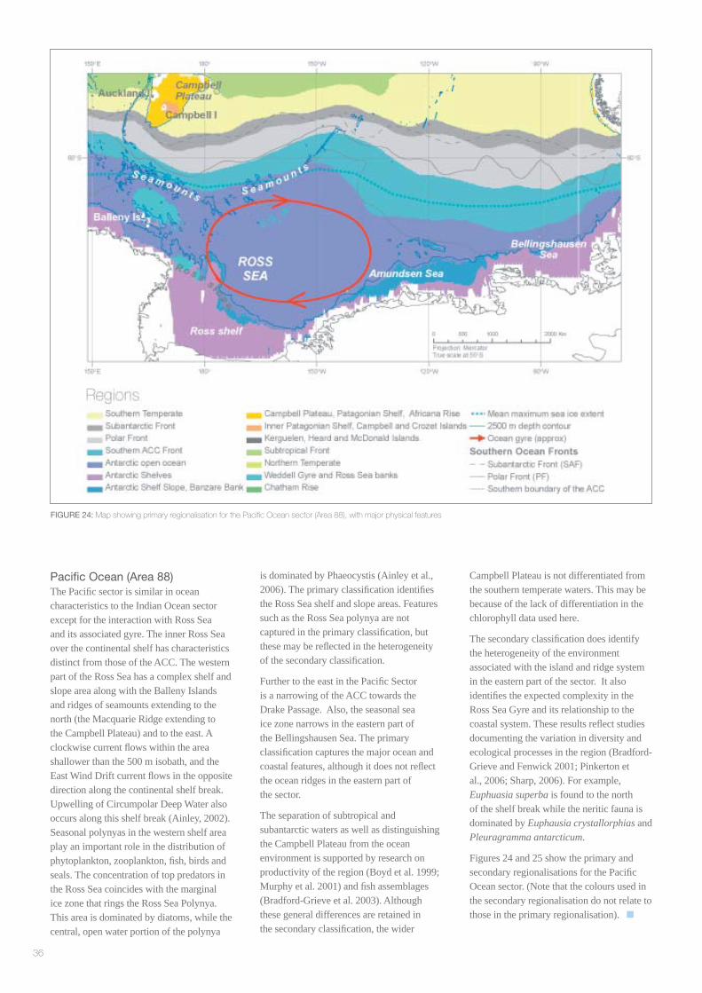
36

Pacifi c Ocean (Area 88)The Pacifi c sector is similar in ocean characteristics to the Indian Ocean sector except for the interaction with Ross Sea and its associated gyre. The inner Ross Sea over the continental shelf has characteristics distinct from those of the ACC. The western part of the Ross Sea has a complex shelf and slope area along with the Balleny Islands and ridges of seamounts extending to the north (the Macquarie Ridge extending to the Campbell Plateau) and to the east. A clockwise current fl ows within the area shallower than the 500 m isobath, and the East Wind Drift current fl ows in the opposite direction along the continental shelf break. Upwelling of Circumpolar Deep Water also occurs along this shelf break (Ainley, 2002). Seasonal polynyas in the western shelf area play an important role in the distribution of phytoplankton, zooplankton, fi sh, birds and seals. The concentration of top predators in the Ross Sea coincides with the marginal ice zone that rings the Ross Sea Polynya. This area is dominated by diatoms, while the central, open water portion of the polynya

is dominated by Phaeocystis (Ainley et al., 2006). The primary classifi cation identifi es the Ross Sea shelf and slope areas. Features such as the Ross Sea polynya are not captured in the primary classifi cation, but these may be refl ected in the heterogeneity of the secondary classifi cation.

Further to the east in the Pacifi c Sector is a narrowing of the ACC towards the Drake Passage. Also, the seasonal sea ice zone narrows in the eastern part of the Bellingshausen Sea. The primary classifi cation captures the major ocean and coastal features, although it does not refl ect the ocean ridges in the eastern part of the sector.

The separation of subtropical and subantarctic waters as well as distinguishing the Campbell Plateau from the ocean environment is supported by research on productivity of the region (Boyd et al. 1999; Murphy et al. 2001) and fi sh assemblages (Bradford-Grieve et al. 2003). Although these general differences are retained in the secondary classifi cation, the wider

Campbell Plateau is not differentiated from the southern temperate waters. This may be because of the lack of differentiation in the chlorophyll data used here.

The secondary classifi cation does identify the heterogeneity of the environment associated with the island and ridge system in the eastern part of the sector. It also identifi es the expected complexity in the Ross Sea Gyre and its relationship to the coastal system. These results refl ect studies documenting the variation in diversity and ecological processes in the region (Bradford-Grieve and Fenwick 2001; Pinkerton et al., 2006; Sharp, 2006). For example, Euphuasia superba is found to the north of the shelf break while the neritic fauna is dominated by Euphausia crystallorphias and Pleuragramma antarcticum.

Figures 24 and 25 show the primary and secondary regionalisations for the Pacifi c Ocean sector. (Note that the colours used in the secondary regionalisation do not relate to those in the primary regionalisation).

FIGURE 24: Map showing primary regionalisation for the Pacifi c Ocean sector (Area 88), with major physical features

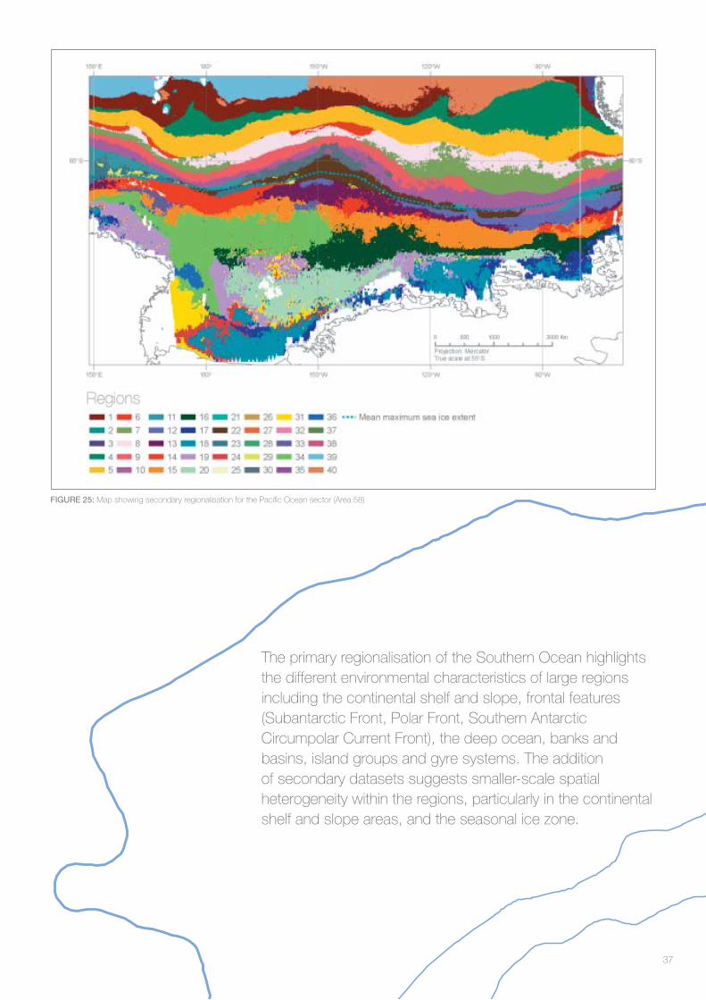
37

FIGURE 25: Map showing secondary regionalisation for the Pacifi c Ocean sector (Area 58)

The primary regionalisation of the Southern Ocean highlights the different environmental characteristics of large regions including the continental shelf and slope, frontal features (Subantarctic Front, Polar Front, Southern Antarctic Circumpolar Current Front), the deep ocean, banks and basins, island groups and gyre systems. The addition of secondary datasets suggests smaller-scale spatial heterogeneity within the regions, particularly in the continental shelf and slope areas, and the seasonal ice zone.

38

Lyn

Irvin

e, A

ustr

alia

n G

over

nmen

t Ant

arct

ic D

ivis

ion,

© C

omm

onw

ealth

of A

ustr

alia

39

The workshop identifi ed a range of areas in which future work might be directed in order to produce a fi nal bioregionalisation for the Southern Ocean. Priorities included the incorporation of additional (particularly biological) datasets, and fi ner-scale analysis of particular areas of interest. It also identifi ed that the statistical methods might be refi ned further. However, the workshop was satisfi ed that the proof of concept developed is suffi cient to undertake the tasks identifi edby CCAMLR and the CEP.

Further data could be used to update or refi ne the draft broad-scale primary regionalisation (for example using additional datasets such as insolation (PAR) and sea surface height). Datasets used in this analysis might also be refi ned, for example using derived datasets such as a ‘silicate depletion’ data layer (refl ective of primary production) derived by subtracting silicate at the surface from silicate at 200 m depth.The remotely-sensed PAR data are confounded by the inability to distinguish ice cover from cloud cover, however they might be transformed to represent biologically relevant variation in available light, by combining PAR data and ice data.

The addition of sea ice and chlorophyll a datasets in the exploratory secondary classifi cations illustrated the high level of heterogeneity arising from these parameters. Refi nement of the analysis and data used at the secondary classifi cation level is needed to identify the appropriate level of regional separation at a smaller scale using these secondary datasets, and to identify whether

other datasets could be used to assist this process. In particular, sea ice is a major driver of ecosystem processes in the Southern Ocean (see Section 1.3), and the inclusion of variables representing sea ice dynamics will be important in fi ner-scale regionalisation analyses.

The draft regionalisation presented in this report is pelagic, however it may also be necessary to undertake a benthic regionalisation. Further consideration should be given to the relationships between the benthic and pelagic systems, and the utility of separating the two systems in the context of bioregionalisation analysis.

A range of potential biological datasets (for use in future analyses) were identifi ed during the workshop (see Appendix V), but it will be necessary to identify which of these would be of most value. Data ‘compendia’ may be of assistance in providing information on inter-annual and seasonal variability, which can then be further analysed according to the defi ned objectives. Indicator species might also be investigated for their potential utility in providing further input to the analysis. In the longer term, the compilation of comprehensive biological data sets may allow the use of more sophisticated analytical approaches such as Generalised Dissimilarity Modelling (GDM – Ferrier et al. in press). This performs an integrated statistical analysis of biological and environmental data, using information on species turnover rates to identify the optimal weighting and transformation of environmental variables to

be used in defi ning the classifi cation.

It may be important to consider stochastic, temporal or spatial variability in defi ning bioregions in order to ensure that the outcome is robust to uncertainties and variability. Further work towards understanding (and, where possible, reducing) different types of uncertainty in the data, models or methods will help the classifi cation process.

A bioregionalisation will inevitably be based on the best scientifi c evidence available at the time. Further refi nement could be achieved by adding biological and environmental data as it becomes available, thereby reducing uncertainties. One source of refi nement will be to add more biological data to test the relationship between physical and environmental surrogates and the ecological processes they are thought to represent. This is likely to be needed at fi ner-scale resolution of the bioregionalisation.

The most important avenue for further work will be to undertake a fi ner-scale regionalisation than that presented here. This might initially be focused in areas where more data is available, such as in the southwest Atlantic. The addition of datasets on chlorophyll a and sea ice extent illustrated the complexity of the coastal, shelf and seasonal ice areas, in relation to these parameters. These regions are likely to have additional complexity corresponding to other ecological processes and species distributions, and should be a priority for further research.

4. Future work

This workshop established a ‘proof of concept’ for bioregionalisation of the Southern Ocean. Further work within the frameworks of CCAMLR and the CEP will be an important contribution to the achievement of a range of scientifi c, management and conservation objectives, including large-scale ecological modelling, ecosystem-based management of human activities in the marine environment, and the development of ecologically representative protected area systems. Continuing work on this topic also has the potential to inform and contribute to the further development of bioregionalisation analysis as a tool for conservation and management in the global context.

5. Conclusions

40

APPENDIX I: Approaches to bioregionalisation – examples presented during

the workshop

• Antarctic Environmental Domains Analysis (Harry Keys and Fraser Morgan,

Department of Conservation, New Zealand)

• CCAMLR Small-Scale Management Units for the fi shery on Antarctic krill in the

Southwest Atlantic (Roger Hewitt, NOAA, USA)

• Australian National Bioregionalisation: Pelagic Regionalisation (Vincent Lyne and

Donna Hayes, Department of the Environment and Heritage and CSIRO)

• Selecting Marine Protected Areas in New Zealand’s EEZ (John Leathwick, NIWA,

New Zealand)

APPENDIX II: Technical information on approach to bioregionalisation

APPENDIX III: Descriptions of datasets used in the analysis

APPENDIX IV: Results of secondary regionalisation using ice and chlorophyll data

APPENDIX V: Biological datasets of potential use in further bioregionalisation work

APPENDIX VI: Details of datasets, Matlab code and ArcGIS shapefi les included

on the CD

List of Appendices (provided on CD)

41

PARTICIPANT EXPERTISE AFFILIATION

Dr. Ian Ball Mathematical modelling, ACE CRC, MPA selection AGAD, Australia

Ms. Kendall Benton Support WWF-Australia

Dr. Andrew Constable Chair, ecosystem ecology ACE CRC, and modelling, marine AGAD, Australia protected areas, CCAMLR

Dr. Susan Doust Support, CCAMLR AGAD, Australia

Dr. Susie Grant Support, marine protected UK areas, CCAMLR, CEP

Dr. Roger Hewitt Krill biology, ecosystem SW Fisheries Centre, ecology NOAA, USA

Dr. Graham Hosie Zooplankton ecology; AGAD, Australia CPR program SCAR representative

Dr. So Kawaguchi Krill biology, ACE CRC, AGAD, ecosystem ecology Australia

Dr. Harry Keys Bioregionalisation, Antarctic DOC, NZ regional classifi cation

Dr. John Leathwick Statistical modelling, NIWA, bioregionalisation, MPA selection Hamilton, NZ

Dr. Gilly Llewellyn Support, classifi cation, WWF-Australia regionalisation, marine protected areas

Dr. Vincent Lynne Statistician, bioregionalisation CSIRO MAR, Hobart, Australia

Dr. Enrique Marschoff Krill biologist (larvae), CCAMLR Argentina

Dr. Rob Massom Sea ice, remote sensing ACE CRC, Australia

Mr. Ewan McIvor Environmental policy AGAD, Australia

Dr. Denzil Miller Observer CCAMLR Secretariat

Dr. Mikio Naganobu Krill biology, ecosystem ecology Japan

Dr. Steve Nicol Krill biology, ecosystem ecology ACE CRC, AGAD, Australia

Dr. Matt Pinkerton Ecosystem modelling, NIWA, NZ remote sensing

Dr. Ben Raymond Modelling, data visualisation ACE CRC, AGAD, Australia

Dr. Steve Rintoul Physical oceanography, ACE CRC, Australia remote sensing

Dr. Eugene Sabourenkov Observer CCAMLR Secretariat

Dr. Ben Sharp Marine biologist, marine MFish, NZ protected area research

Dr. Sergei Sokolov Physical oceanography, ACE CRC, Australia remote sensing

Mr. Rick Smith Statistician, bioregionalisation CSIRO MAR, Hobart, Australia

Dr. Pete Strutton Primary production, Oregon State remote sensing University, USA

Dr. Phil Trathan Ecosystem and predator BAS, UK ecology, CCAMLR

List of workshop participants

42

Bioregionalisation (or Regionalisation)

A process that aims to partition a broad spatial area into distinct spatial regions, using a range of environmental and biological information. The process results in a set of bioregions, each with relatively homogeneous and predictable ecosystem properties. The properties of a given bioregion should differ from those of adjacent regions in terms of species composition as well as the attributes of its physical and ecological habitats. The term regionalisation may be used interchangeably (or sometimes to refer to an analysis undertaken using only physical data).

Bioregion (or Region)

A spatial compartment defi ned on the basis of its biological and/or physical properties. Each bioregion (or region) refl ects a unifying set of major environmental infl uences which shape the occurrence of biota and their interaction with the physical environment. The term region may be used interchangeably (or sometimes to refer to spatial compartments which have been defi ned using only physical data).

Classifi cation

The process of partitioning a broad spatial area into distinct regions. Also used to refer to the specifi c step within that process during which the actual allocation of sites to regions occurs, usually through a statistical process such as cluster analysis

Ecological process

In the context of this report, an ecological process is any process that affects the dynamics of a species

Hierarchy (spatial and statistical)

In the context of bioregionalisation, this term may be used to refer to spatial or ecological hierarchy, or statistical hierarchy.

Spatial or ecological hierarchy refers to the different levels of scale or ecological processes within a large area. A hierarchy may be nested, whereby smaller scale units or processes are nested within large scale units.

Statistical hierarchy has relevance in dissimilarity-based clustering methods, where an iterative approach is undertaken to group sites together into regions. All sites are initially allocated to their own regions. At each iteration of the process (or each step down the hierarchy), the two most similar regions are merged together, until at the end of the process there is only one region, which contains all of the sites. This is often displayed in dendograms.

Glossary of terms

Parameter

Information extracted from data. For example, sea ice concentration is a variable from which the parameters of ‘proportion of year when the ocean is covered by at least 15% ice’ or ‘areas with greater than 50% ice coverage’ can be extracted.

Property

This term is used here to describe the defi ning characteristics or attributes of a particular ecological process, or of a given region.

Proxy

A parameter that can be used to provide similar information or patterns to another parameter or variable, usually used when desired data (e.g. the distribution of species) are unavailable, or where one parameter can be used in the place of several others in order to simplify the analysis.

Site

In the context of bioregionalisation analysis, a site is the smallest unit of analysis. The study area is divided into a grid of sites, at suffi ciently fi ne scale to enable appropriate resolution of the fi nal areas. Each site will have a particular set of parameters, according to the input data.

Synoptic

This term is used to describe data that have broad and continuous spatial coverage (e.g. across the entire Southern Ocean). Here, synoptic data may also refer to summaries of the observed conditions over time (e.g. mean monthly values averaged to obtain an annual mean). Synoptic data may be obtained through satellite remote-sensing, or through model climatologies generated from observed values.

Uncertainty

In the context of bioregionalisation analysis, uncertainty refers to the effects of imprecision in data (e.g. measurement error), uncertainty within models used to derive variables (e.g. climatology models), and epistemic uncertainty (potential errors in the chosen method). Each of these types of uncertainty can affect the resulting region boundaries.

Variable

Variables are physical or environmental data from which specifi c parameters can be extracted. For example, sea ice concentration is a variable from which the parameters of ‘proportion of year when the ocean is covered by at least 15% ice’ or ‘areas with greater than 50% ice coverage’ can be extracted.

43

References

Ackley, S.F., and Sullivan, C.W. (1994) Physical controls on the development and characteristics of Antarctic sea ice biological communities a review and synthesis. Deep-Sea Research 41(10): 1583 1604

Ainley, D.G. (2002) The Ross Sea, Antarctica, where all ecosystem processes still remain for study, but maybe not for long. Marine Ornithology 30: 55-62

Ainley, D. G., Tynan, C.T. and Stirling, I. (2003) Sea ice: A critical habitat for polar marine mammals and birds. In D. Thomas and G. Dieckmann (eds), Sea Ice – An Introduction to its Physics, Biology, Chemistry and Geology. Blackwell Science, Oxford, pp. 240-266.

Ainley, D., Toniolo, V., Ballard, G., Barton, K., Eastman, J., Karl, B., Focardi, S., Kooyman, G., Lyver, P., Olmastroni, S., Stewart, B.S., Testa J.W. and Wilson, P. (2006) Managing ecosystem uncertainty: critical habitat and dietary overlap of top-predators in the Ross Sea. WG-EMM-06/29.

Amos, F.A. (2001) A decade of oceanographic variability in summertime near Elephant Island, Antarctica. Journal of Geophysical Research 106 (C10): 22401–22423.

Andrewartha, H.G. and Birch, L. C. (1984) The ecological web: more on the distribution and abundance of animals. University of Chicago Press, Chicago.

Arrigo, K.R., and van Dijken, G.L. (2003) Phytoplankton dynamics within 37 Antarctic coastal polynya systems. J. Geophys. Res. 108(C8): 3271. doi:10.1029/2002JC001739.

ATCM XXIV/WP012 (2001) Systematic Environmental-Geographic Framework for Protected Areas under Annex V of the Environmental Protocol. Antarctic Treaty Consultative Meeting XXIV. Working Paper No. 12.

Atkinson, A. and Sinclair, J.D. (2000) Zonal distribution and seasonal vertical migration of copepod assemblages in the Scotia Sea. Polar Biology 23(1): 46-58

Atkinson, A., Siegel, V., Pakhomov, E. and Rothery, P. (2004) Long-term decline in krill stock and increase in salps within the Southern Ocean. Nature 432 (7013): 100-103

Bailey, R.G. (1996) Ecosystem Geography. Springer-Verlag, New York.

Beaman R.J. and Harris P.T. (2005) Bioregionalization of the George V Shelf, East Antarctica. Continental Shelf Research 25:1657–1691

Belbin, L. (1993) Environmental representativeness: regional partitioning and reserve selection. Biological Conservation 66: 223–230.

Bindoff, N. L., Rintoul, S.R. and Massom R. (2000). Polynyas and bottom water formation south of Tasmania. Papers and Proceedings of the Royal Society of Tasmania, 133(3), 51–56

Boyd, P.W., LaRoche, J., Gall, M., Frew, R. and McKay, R. (1999) Role of iron, light, and silicate in controlling algal biomass in subantarctic waters SE of New Zealand. Journal of Geophysical Research 104, C6, pp 13391-13404.

Bradford-Grieve, J. and Fenwick, G. (2001) A review of the current knowledge describing the biodiversity of the Ross Sea. Final research report for Ministry of Fisheries, Research Project ZBD2000/01 Objective 1 (in part). 93 pp.

Bradford-Grieve, J.M., Probert, P.K., Nodder, S.D., Thompson, D., Hall, J., Hanchet, S., Boyd, P., Zeldis, J., Baker, A.N., Best, H.A., Broekhuizen, N., Childerhouse, S., Clark, M., Hadfi eld, M., Safi , K. and Wilkinson, I. (2003) Pilot trophic model for subantarctic water over the Southern Plateau, New Zealand: a low biomass, high transfer effi ciency system. Journal of Experimental Marine Biology and Ecology 289: 223-262.

Brierley, A.S., and Thomas, D.N. (2002) Ecology of Southern Ocean pack ice. Advances in Marine Ecology 43: 171-276

Casey, K.S. and Cornillon, P. (1999) A comparison of satellite and in situ based sea surface temperature climatologies, J. Climate, 12 (6): 1848-1863. http://podaac-www.jpl.nasa.gov/products/product112.html

CEP IX (2006) Report of the Committee for Environmental Protection (CEP IX). Edinburgh, 2006.

Chiba, S., Ishimaru, T., Hosie, G.W., Wright, S.W. (1999) Population structure change of Salpa thompsoni from austral mid-summer to autumn. Polar Biology 22: 341-349

Chiba, S., Ishimaru, T., Hosie, G.W., Fukuchi, M. (2001) Spatio-temporal variability of zooplankton community structure in the western Pacifi c Ocean sector, Antarctica. Marine Ecology Progress Series 216: 95-108.

Clarke, A. (1996) Distribution of Antarctic marine benthic communities. In: Ross, R.M., Hofmann, E.E. & Quetin, L.B. Foundations for Ecological Research West of the Antarctic Peninsula. American Geophysical Union, Washington. (pp. 219-230).

Clarke, A. and Johnston, N.M. (2003) Antarctic Marine Benthic Diversity. Oceanography and Marine Biology: an Annual Review 41: 47-114.

Comiso, J. (1999), updated 2005. Bootstrap sea ice concentrations for NIMBUS-7 SMMR and DMSP SSM/I. Boulder, CO, USA: National Snow and Ice Data Center. Digital media. http://nsidc.org/data/nsidc-0079.html

Constable, A.J. and Nicol, S. (2002) Defi ning smaller-scale management units to further develop the ecosystem approach in managing large-scale pelagic krill fi sheries in Antarctica. CCAMLR Science 9: 117–131.

Dell, R.K. (1972) Antarctic benthos. Advances in Marine Biology 10: 1-216.

Eicken, H. (1992) The role of sea ice in structuring Antarctic ecosystems. Polar Biology 12: 3-13

Ekman, V.K. (1953) Zoogeography of the Sea. Sidgwick and Jackson, London.

Everson, I. (1977) The living resources of the Southern Ocean. Food and Agriculture Organisation, GLO/S0/77/1. Rome.

Ferrier, S., Manion, G., Elith, J., and Richardson, K. in press. Using generalised dissimilarity modelling to analyse and predict patterns of beta-diversity in regional biodiversity assessment. Diversity and Distributions.

Faith, D.P., Minchin, P.R., and Belbin, L. (1987) Compositional dissimilarity as a robust measure of ecological distance. Vegetation 69:57-68.

Fowler, C. (2003) Polar Pathfi nder Daily 25 km EASE-Grid Sea Ice Motion Vectors. US National Snow and Ice Data Center, Boulder, Colorado, USA. Digital media.

Frouin, R., Franz, B. and Wang, M. Algorithm to estimate PAR from SeaWiFS data Version 1.2 – Documentation. http://oceancolor.gsfc.nasa.gov/DOCS/seawifs_par_algorithm.pdf

Garrison, D.L. and Mathot, S. (1996) Pelagic and sea ice microbial communities. In Foundations for Ecological Research West of the Antarctic Peninsula, Ross, R.M., Hofmann, E.E. and Quetin, L.B. (Eds) American Geophysical Union, Antarctic Research Series, 70, pp. 155-172

44

Gloersen, P., Campbell, W.J., Cavalieri, D.J., Comiso, J.G., Parkinson, C.L. and Zwally, H.J. (1992). Arctic and Antarctic sea ice, 1978 1987: Satellite passive microwave observa¬tions and analysis. NASA Special Publication SP 511, NASA, Washington D.C., USA, 290 pp.

Gouretski, V.V. and Koltermann, K. P. (2004) WOCE Global Hydrographic Climatology. Technical Report, 35, Berichte des Bundesamtes für Seeschifffahrt und Hydrographie. http://odv.awi-bremerhaven.de/data/ocean/woce-global-hydrographic-climatology.html

Hayes, D., Lyne, V., Condie, S., Griffi ths, B., Pigot, S. and Hallegraef, G. (2005) Collation and Analysis of Oceanographic Datasets for National Marine Bioregionalisation. CSIRO Report to the National Oceans Offi ce. CSIRO Marine Research, Hobart.

Hedgpeth, J.W. (1970) Marine biogeography of the Antarctic regions. In: Holdgate, M.W. (ed.) Antarctic Ecology (Volume 1) Academic Press, London. (pp. 97-104)

Hewitt, R.P., Watkins, J.L., Naganobu, M., Tshernyshkov, P., Brierley, A.S., Demer, D.A., Kasatkina, S., Takao, Y., Goss, C., Malyshko, A., Brandon, M.A., Kawaguchi, S., Siegel, V., Trathan, P.N., Emery, J.H., Everson, I. and Miller, D.G.M. (2002) Setting a precautionary catch limit for Antarctic krill. Oceanography 15(3): 26–33.

Hewitt, R.P., Watters, G., Trathan, P.N., Croxall, J.P., Goebel, M.E., Reid, K., Trivelpiece, W.Z. and Watkins, J.L. (2004). Options for allocating the precautionary catch limit of krill among Small-Scale Management Units in the Scotia Sea. CCAMLR Science 11: 81-98.

Hoddell, R.J., Crossley, A.C., Williams, R. and Hosie, G.W. (2000) The Distribution of Antarctic Pelagic Fish and Larvae (CCAMLR Division 58.4.1) Deep Sea Research 47(12-13): 2519-2541

Hosie, G.W. (1991) Distribution and abundance of euphausiid larvae in the Prydz Bay region, Antarctica (January 1985). Antarctic Science 3(2):167-180

Hosie, G.W. (1994a) The macrozooplankton communities in the Prydz Bay region, Antarctica. In: S.Z. El-Sayed (ed) Southern Ocean Ecology: The BIOMASS Perspective. Cambridge University Press pp 93-123.

Hosie, G.W. (1994b) Multivariate analyses of the macrozooplankton community and euphausiid larval ecology in the Prydz Bay region, Antarctica. ANARE Reports 137.

Hosie, G.W., Cochran, T.G., Pauly, T., Beaumont, K.L., Wright, S.W., Kitchener, J.A. (1997) The zooplankton community structure of Prydz Bay, January-February 1993. Proceedings of the NIPR Symposium on Polar Biology 10: 90-133.

Hosie, G.W., Schultz, M.B., Kitchener, J.A.,Cochran, T.G. and Richards, K. (2000) Zooplankton community structure off East Antarctica (80-150° east) during the Austral summer of 1995/96. Deep Sea Research 47(12-13): 2437-2463

Hosie, G.W., Fukuchi, M. and Kawaguchi, S. (2003) Development of the Southern Ocean Continuous Plankton Recorder Survey. Progress in Oceanography 58(2-4): 263-283

Hunt, B.P.V. and Hosie, G.W. (2003) The Continuous Plankton Recorder in the Southern Ocean: a comparative analysis of zooplankton communities sampled by the CPR and vertical net hauls along 140°E. Journal of Plankton Research 25(12): 1-19

Hunt, B.P.V. and Hosie, G.W. (2005) Zonal Structure of Zooplankton Communities in the Southern Ocean south of Australia: results from a 2150 kilometre Continuous Plankton Recorder transect. Deep-Sea Research I 52: 1241-1271.

Hunt, B.P.V. and Hosie, G.W. (2006a) Seasonal zooplankton community succession in the Southern Ocean south of Australia, Part I: The Seasonal Ice Zone. Deep-Sea Research I 53: 1182-1202

Hunt, B.P.V. and Hosie, G.W. (2006b) Seasonal zooplankton community succession in the Southern Ocean south of Australia, Part II: The Sub-Antarctic to Polar Frontal Zones. Deep-Sea Research I 53: 1203-1223

Ichii, T. (1990) Distribution of Antarctic krill concentrations exploited by Japanese krill trawlers and minke whales. Proceedings of the NIPR Symposium on Polar Biology 3: 36-56

IOC, IHO and BODC, 2003. Centenary Edition of the GEBCO Digital Atlas, published on CD-ROM on behalf of the Intergovernmental Oceanographic Commission and the International Hydrographic Organization as part of the General Bathymetric Chart of the Oceans, British Oceanographic Data Centre, Liverpool, U.K.

Kaufman, L. and Rousseeuw, P.J. Finding Groups in Data. An Introduction to Cluster Analysis. John Wiley & Sons, New York, 1990.

Knox, G.A. (1994) The Biology of the Southern Ocean. Cambridge, Cambridge University Press, 444 p.

Kock, K.-H. (2000) Understanding CCAMLR’s approach to management. CCAMLR, Hobart, Australia.

Kwok, R. and Comiso, J.C. (2002) Southern Ocean climate and sea ice anomalies associated with the Southern Oscillation. Journal of Climate 15(5): 487-501.

Leathwick, J.R., Dey, K. and Julian, K. (2006a) Development of an environmental classifi cation optimised for demersal fi sh. NIWA Client Report HAM2006-063.

Leathwick, J.R., Francis, M.P. and Julian, K. (2006b) Development of a demersal fi sh community map of New Zealand’s Exclusive Economic Zone. NIWA Client Report HAM2006-062.

Leathwick, J.R., Julian, K. and Francis, M.P. (2006c) Exploration of the use of reserve planning software to identify potential Marine Protected Areas in New Zealand’s Exclusive Economic Zone. NIWA Client Report HAM2006-064.

Leathwick, J.R., Overton, J. McC. and McLeod, M. (2003) An environmental domain classifi cation of New Zealand and its use as a tool for biodiversity management. Conservation Biology 17: 1612–1623

Legendre, L., Ackley, S.F., Dieckmann, G.S., Gullicksen, B., Homer, R., Hoshiai, T., Melnikov, I.A., Reeburgh, W.S., Spindler, M. and Sullivan, C.W. (1992) Ecology of sea ice biota: 2. Global Signifi cance. Polar Biology 12: 429 444

Linse, K., Griffi ths, H.J., Barnes, D.K.A. and Clarke, A. (2006) Biodiversity and biogeography of Antarctic and sub-Antarctic mollusca. Deep Sea Research II 53: 985-1008.

Lizotte, M.P. (2001) The contributions of sea ice algae to Antarctic marine primary production. American Zoologist 41(1): 57-73

Lizotte, M. P. and Arrigo, K.R. (eds) (1998) Antarctic Sea Ice: Biological Processes, Interactions, and Variability. Antarctic Research Series 73, American Geophysical Union, Washington DC.

Longhurst, A.R. (1998) Ecological Geography of the Sea. Academic Press, Florida.

Lyne, V and Hayes, D. (2005) Pelagic Regionalisation: National Marine Bioregionalisation Integration Project. CSIRO Report to the National Oceans Offi ce. CSIRO Marine Research, Hobart. (Summary)

Massom, R. A. (2003) Recent iceberg calving events in the Ninnis Glacier region, East Antarctica, Ant. Sc., 15(2): 303-313

Massom, R. A., Harris, P.T., Michael, K.J. and Potter, M.J. (1998) The distribution and formative processes of latent-heat polynyas in East Antarctica. Ann. Glaciol., 27: 420-426

References

44

References

Gloersen, P., Campbell, W.J., Cavalieri, D.J., Comiso, J.G., Parkinson, C.L. and Zwally, H.J. (1992). Arctic and Antarctic sea ice, 1978 1987: Satellite passive microwave observa¬tions and analysis. NASA Special Publication SP 511, NASA, Washington D.C., USA, 290 pp.

Gouretski, V.V. and Koltermann, K. P. (2004) WOCE Global Hydrographic Climatology. Technical Report, 35, Berichte des Bundesamtes für Seeschifffahrt und Hydrographie. http://odv.awi-bremerhaven.de/data/ocean/woce-global-hydrographic-climatology.html

Hayes, D., Lyne, V., Condie, S., Griffi ths, B., Pigot, S. and Hallegraef, G. (2005) Collation and Analysis of Oceanographic Datasets for National Marine Bioregionalisation. CSIRO Report to the National Oceans Offi ce. CSIRO Marine Research, Hobart.

Hedgpeth, J.W. (1970) Marine biogeography of the Antarctic regions. In: Holdgate, M.W. (ed.) Antarctic Ecology (Volume 1) Academic Press, London. (pp. 97-104)

Hewitt, R.P., Watkins, J.L., Naganobu, M., Tshernyshkov, P., Brierley, A.S., Demer, D.A., Kasatkina, S., Takao, Y., Goss, C., Malyshko, A., Brandon, M.A., Kawaguchi, S., Siegel, V., Trathan, P.N., Emery, J.H., Everson, I. and Miller, D.G.M. (2002) Setting a precautionary catch limit for Antarctic krill. Oceanography 15(3): 26–33.

Hewitt, R.P., Watters, G., Trathan, P.N., Croxall, J.P., Goebel, M.E., Reid, K., Trivelpiece, W.Z. and Watkins, J.L. (2004). Options for allocating the precautionary catch limit of krill among Small-Scale Management Units in the Scotia Sea. CCAMLR Science 11: 81-98.

Hoddell, R.J., Crossley, A.C., Williams, R. and Hosie, G.W. (2000) The Distribution of Antarctic Pelagic Fish and Larvae (CCAMLR Division 58.4.1) Deep Sea Research 47(12-13): 2519-2541

Hosie, G.W. (1991) Distribution and abundance of euphausiid larvae in the Prydz Bay region, Antarctica (January 1985). Antarctic Science 3(2):167-180

Hosie, G.W. (1994a) The macrozooplankton communities in the Prydz Bay region, Antarctica. In: S.Z. El-Sayed (ed) Southern Ocean Ecology: The BIOMASS Perspective. Cambridge University Press pp 93-123.

Hosie, G.W. (1994b) Multivariate analyses of the macrozooplankton community and euphausiid larval ecology in the Prydz Bay region, Antarctica. ANARE Reports 137.

Hosie, G.W., Cochran, T.G., Pauly, T., Beaumont, K.L., Wright, S.W., Kitchener, J.A. (1997) The zooplankton community structure of Prydz Bay, January-February 1993. Proceedings of the NIPR Symposium on Polar Biology 10: 90-133.

Hosie, G.W., Schultz, M.B., Kitchener, J.A.,Cochran, T.G. and Richards, K. (2000) Zooplankton community structure off East Antarctica (80-150° east) during the Austral summer of 1995/96. Deep Sea Research 47(12-13): 2437-2463

Hosie, G.W., Fukuchi, M. and Kawaguchi, S. (2003) Development of the Southern Ocean Continuous Plankton Recorder Survey. Progress in Oceanography 58(2-4): 263-283

Hunt, B.P.V. and Hosie, G.W. (2003) The Continuous Plankton Recorder in the Southern Ocean: a comparative analysis of zooplankton communities sampled by the CPR and vertical net hauls along 140°E. Journal of Plankton Research 25(12): 1-19

Hunt, B.P.V. and Hosie, G.W. (2005) Zonal Structure of Zooplankton Communities in the Southern Ocean south of Australia: results from a 2150 kilometre Continuous Plankton Recorder transect. Deep-Sea Research I 52: 1241-1271.

Hunt, B.P.V. and Hosie, G.W. (2006a) Seasonal zooplankton community succession in the Southern Ocean south of Australia, Part I: The Seasonal Ice Zone. Deep-Sea Research I 53: 1182-1202

Hunt, B.P.V. and Hosie, G.W. (2006b) Seasonal zooplankton community succession in the Southern Ocean south of Australia, Part II: The Sub-Antarctic to Polar Frontal Zones. Deep-Sea Research I 53: 1203-1223

Ichii, T. (1990) Distribution of Antarctic krill concentrations exploited by Japanese krill trawlers and minke whales. Proceedings of the NIPR Symposium on Polar Biology 3: 36-56

IOC, IHO and BODC, 2003. Centenary Edition of the GEBCO Digital Atlas, published on CD-ROM on behalf of the Intergovernmental Oceanographic Commission and the International Hydrographic Organization as part of the General Bathymetric Chart of the Oceans, British Oceanographic Data Centre, Liverpool, U.K.

Kaufman, L. and Rousseeuw, P.J. Finding Groups in Data. An Introduction to Cluster Analysis. John Wiley & Sons, New York, 1990.

Knox, G.A. (1994) The Biology of the Southern Ocean. Cambridge, Cambridge University Press, 444 p.

Kock, K.-H. (2000) Understanding CCAMLR’s approach to management. CCAMLR, Hobart, Australia.

Kwok, R. and Comiso, J.C. (2002) Southern Ocean climate and sea ice anomalies associated with the Southern Oscillation. Journal of Climate 15(5): 487-501.

Leathwick, J.R., Dey, K. and Julian, K. (2006a) Development of an environmental classifi cation optimised for demersal fi sh. NIWA Client Report HAM2006-063.

Leathwick, J.R., Francis, M.P. and Julian, K. (2006b) Development of a demersal fi sh community map of New Zealand’s Exclusive Economic Zone. NIWA Client Report HAM2006-062.

Leathwick, J.R., Julian, K. and Francis, M.P. (2006c) Exploration of the use of reserve planning software to identify potential Marine Protected Areas in New Zealand’s Exclusive Economic Zone. NIWA Client Report HAM2006-064.

Leathwick, J.R., Overton, J. McC. and McLeod, M. (2003) An environmental domain classifi cation of New Zealand and its use as a tool for biodiversity management. Conservation Biology 17: 1612–1623

Legendre, L., Ackley, S.F., Dieckmann, G.S., Gullicksen, B., Homer, R., Hoshiai, T., Melnikov, I.A., Reeburgh, W.S., Spindler, M. and Sullivan, C.W. (1992) Ecology of sea ice biota: 2. Global Signifi cance. Polar Biology 12: 429 444

Linse, K., Griffi ths, H.J., Barnes, D.K.A. and Clarke, A. (2006) Biodiversity and biogeography of Antarctic and sub-Antarctic mollusca. Deep Sea Research II 53: 985-1008.

Lizotte, M.P. (2001) The contributions of sea ice algae to Antarctic marine primary production. American Zoologist 41(1): 57-73

Lizotte, M. P. and Arrigo, K.R. (eds) (1998) Antarctic Sea Ice: Biological Processes, Interactions, and Variability. Antarctic Research Series 73, American Geophysical Union, Washington DC.

Longhurst, A.R. (1998) Ecological Geography of the Sea. Academic Press, Florida.

Lyne, V and Hayes, D. (2005) Pelagic Regionalisation: National Marine Bioregionalisation Integration Project. CSIRO Report to the National Oceans Offi ce. CSIRO Marine Research, Hobart. (Summary)

Massom, R. A. (2003) Recent iceberg calving events in the Ninnis Glacier region, East Antarctica, Ant. Sc., 15(2): 303-313

Massom, R. A., Harris, P.T., Michael, K.J. and Potter, M.J. (1998) The distribution and formative processes of latent-heat polynyas in East Antarctica. Ann. Glaciol., 27: 420-426

Des

igne

d an

d pr

oduc

ed b

y Fr

esco

Cre

ativ

e: w

ww

.fres

cocr

eativ

e.co

m.a

u

Planning for Representative Marine Protected Areas

A Framework for Canada’s Oceans

ABOUT THE AUTHORS

Jon C. Day, B.Nat.Res. (Hon.)

This report was compiled as a contract task for WWF Canada

while Jon worked temporarily as a marine and coastal consul-

tant in Canada. He is Director of Conservation, Biodiversity and

World Heritage with the Great Barrier Reef Marine Park

Authority.

His previous positions include Regional Manager (Marine and

Coastal) for the Queensland Department of Environment and

Heritage which involved responsibility for managing approxi-

mately one-third of the Great Barrier Reef World Heritage Area

(the world’s largest marine protected area). Jon has had exten-

sive experience as a park planner and park manager during his

27 years working for resource management agencies through-

out Australia, including both federal and state agencies.

Contact address:

Great Barrier Reef Marine Park Authority, PO Box 1379

Townsville, QLD Australia 4810

Phone (07) 4750 0803; Fax (07) 4772-6093;

E-mail jon.day@gbrmpa.gov.au

John C. Roff, B.A., M.A., Ph.D.

John is a professor in the Department of Zoology in the

College of Biological Science at the University of Guelph

and is also currently editor of the Canadian Journal of Fisheries

and Aquatic Sciences. His work has been published widely in

various journals, books and technical reports. John has broad

interests in the aquatic sciences, from developing radiochemi-

cal and biochemical techniques for measuring growth rates in

metazoa to modelling the impacts of coastal morphological

change on marine planktonic and benthic communities. John

has lectured throughout Canada, the U.S., the U.K, the West

Indies and Saudi Arabia and is also currently a research fellow

in the Marine Sciences Research Unit at the University of West

Indies, Jamaica.

Contact address:

Department of Zoology, University of Guelph

50 Stone Road East, Guelph, ON Canada N1G 2W1

Phone (519) 824-4120, ext. 2647; Fax (519) 767-9798;

E-mail jroff@uoguelph.ca

Published April 2000 by World Wildlife Fund Canada (WWF). Any reproduction in full or in part of this publication must mention the title and credit the above-mentioned publisher as the copyrightowner. © text 2000 WWF. All rights reserved.

Citation: Day, J.C. and Roff, J.C. 2000. Planning for RepresentativeMarine Protected Areas: A Framework for Canada’s Oceans. Reportprepared for World Wildlife Fund Canada, Toronto.

Cover photo © M. Strong and M. Buzeta

The material presented in this report does not represent the opinion of WWF Canada concerning the legal status of any land, sea or area.

A copy of this publication can be downloaded at www.wwf.ca/MPA—planning/

Planning for Representative Marine Protected Areas

A Framework for Canada’s Oceans

Written by Jon Day and John Roff. April 2000.

Edited by Josh Laughren.

i ■

List of Tables, Figures and Boxes v

Abbreviations vi

Introduction vii

PART 1 CANADA’S MARINE BIODIVERSITY AND THE NEED FOR MARINE PROTECTED AREAS

1a. Canada’s Marine Biodiversity 2

Introduction 2

What Is Biological Diversity and Why Protect It? 4

Threats to Marine Biodiversity and How MPAs Might Help 5

1b. MPAs and a Representative System 8

Introduction to MPAs 8

What is a Representative System of MPAs? 9

The Broad Context of MPAs 10

Definitions 11

What Are the Potential Benefits of MPAs? 12

How MPAs Can Benefit Endangered, Threatened or Rare Species 15

Conservation of Keystone Species 15

Conservation of Valuable Species 15

Conservation of Marine Mammals 15

Conservation of Unique Habitats 16

Conservation of Biodiversity and Productive Ecosystems 16

Conservation of Intangible Values 17

Benefits of MPAs for Scientific Research 17

Global Recognition of MPAs 17

Why Have So Few MPAs Been Declared in Canada? 18

How Many Benefits Can a Representative System of MPAs Provide? 19

1c. Canada’s Biodiversity Strategy and the Role of MPAs 20

Introduction 20

Canada’s Biodiversity Strategy 20

The Role of MPAs 21

1d. WWF Canada’s Endangered Spaces Campaign 24

Contents

■ ii

PART 2 MARINE SCIENCE AND ECOSYSTEMS

2a.Comparison Between Marine and Terrestrial Ecosystems 28

Introduction 28

Similarities Between Terrestrial and Marine Ecosystems 28

Differences Between Terrestrial and Marine Ecosystems 29

Physical and Biological Differences 29

Human Perspectives and Considerations 32

Biogeochemical Linkages 33

Discussion 34

2b. Defining Enduring and Recurrent Features in the Marine Environment 35

Introduction 35

Biological Factors 37

Failings Common to All Species-Level Approaches to Marine Conservation 39

Oceanographic Factors 40

Water Masses and Salinity 40

Temperature 41

Temperature Gradients, Temperature Anomalies and Upwellings 42

Ice Cover and Ice Scour 43

Segregation of Benthic and Pelagic Realms 53

Water Motions 43

Convergences and Divergences 44

Stratification, Mixing and Nutrients 44

Light Penetration and Turbidity 46

Depth and Pressure 47

Tidal Amplitude and Currents 47

Exposure to Atmosphere and Waves 48

Tsunamis, Storm Surges, Hurricanes and Water Spouts 49

Using Oceanographic Factors in a Marine Classification 49

Physiographic Factors 49

Geological Activities 49

Geographical Position and Latitude 50

Geological History of the Ocean Basin 50

Water Depth 50

Relief (Slope) 51

Planning for

Representative Marine

Protected Areas:

A Framework for

Canada’s Oceans

iii ■

Planning for

Representative Marine

Protected Areas:

A Framework for

Canada’s Oceans

Substrate (Sediment) Particle Size 52

Basin Morphometry (Topography) 53

Geology (Rock Type) 53

Using Physiographic Factors in a Marine Classification 54

Conclusions 54

2c. A Review of the Correspondence Between Biological and Geophysical Factors 55

PART 3 A CLASSIFICATION FOR MARINE CONSERVATION

3a. General Principles of a Hierarchical Classification for Marine Conservation 58

Summary of Key Points 58

Guiding Design Principles 59

3b. A National Classification System for Marine Conservation 61

Level 1: Environment Type 63

Level 2: Geographic Range 64

Level 3: Temperature 65

Arctic Waters 66

Subarctic Waters 66

Boreal Waters 66

Temperate Waters 67

Subtropical Waters 67

Level 4: Sea-Ice Cover 67

Permanent Pack Ice 68

Seasonal Ice 68

Variable Ice 68

No Ice 68

Polynyas 68

Level 5: Segregation of Pelagic and Benthic Realms 68

Level 6: Vertical Segregation 70

Pelagic Realm 70

Benthic Realm 71

Level 7: Mixing and Wave Action 71

Pelagic Stratification 71

Benthic Exposure and Slope 72

Level 8: Benthic Substrate 73

■ iv

Planning for

Representative Marine

Protected Areas:

A Framework for

Canada’s Oceans

3c. Data Requirements for Determining Seascapes 74

Introduction 74

Consideration of Scales for Environmental Management 75

3d. Assumptions, Limitations and Caveats 77

Introduction 77

Assumptions and Limitations 77

Caveats 82

PART 4 PLANNING A NATIONAL SYSTEM OF REPRESENTATIVE MPAs

4a. Guiding Principles for Designing a System of MPAs 84

Introduction 84

Basic Principles for the Selection and Design of MPAs 85

Influence of the Goal of MPAs on Their Selection and Design 86

4b. Selection Criteria for MPAs 88

4c. Ecological Principles and Criteria for Designing a System of MPAs 91

Reserve Size 91

Reserve Networks 92

Reserve Connectivity 93

Reserve Shape 94

Reserve Management Type 95

Reserve Replication and Redundancy 95

4d. Other Selection Criteria for MPAs 97

Benefits of No-Take MPAs 98

Benefits of Multiple-Use MPAs 98

Airspace Above an MPA 99

4e. Special Areas 100

4f. Summary: Guiding Principles for Choosing Individual MPAs 102

4g. Conclusion 104

Appendix 1 105 Case Study: Application of WWF Canada’s National Classification for Marine Conservation to the Scotian Shelf

Glossary 131

References 139

v ■

Planning for

Representative Marine

Protected Areas:

A Framework for

Canada’s Oceans

TABLES, FIGURES AND BOXES

Tables

1. Threats to marine biodiversity 6

2. Factors determining, correlated with or controlling the nature and distribution of marine biota 37

3. A national framework for marine classification 62

4. Data requirements for the classification of marine seascapes in Canada 74

5. Scales of human–marine ecosystem interactions 76

Figures

1. Schematic map of Canada’s marine realm 2

2. Pelagic and benthic zones of the ocean 71

3. Conceptual options for a representative network of MPAs in a marine natural region 90

Boxes

1. Potential benefits of MPAs 13

2. Expected benefits of an appropriate system of no-take marine reserves 14

3. WWF Canada’s minimum protection standard for MPAs 25

4. Proposed criteria for assessing the suitability of an area as an MPA 88

■ vi

Planning for

Representative Marine

Protected Areas:

A Framework for

Canada’s Oceans

ABBREVIATIONS

The following abbreviations have been used in this report:

CNPPA Commission on National Parks and Protected Areas (of IUCN)

COSEWIC Committee on the Status of Endangered Wildlife in Canada

CWS Canadian Wildlife Service

DFO Department of Fisheries and Oceans

EEZ exclusive economic zone

GBRMP Great Barrier Reef Marine Park

GBRMPA Great Barrier Reef Marine Park Authority

GIS geographic information system

GPS global positioning system

ICM integrated coastal management

IMO International Maritime Organization

IUCN World Conservation Union

MPA marine protected area

NMCA National Marine Conservation Area

OMS Oceans Management Strategy

UNCLOS United Nations Convention on the Law of the Sea

UNEP United Nations Environment Program

WCMC World Conservation Monitoring Centre

WWF World Wildlife Fund

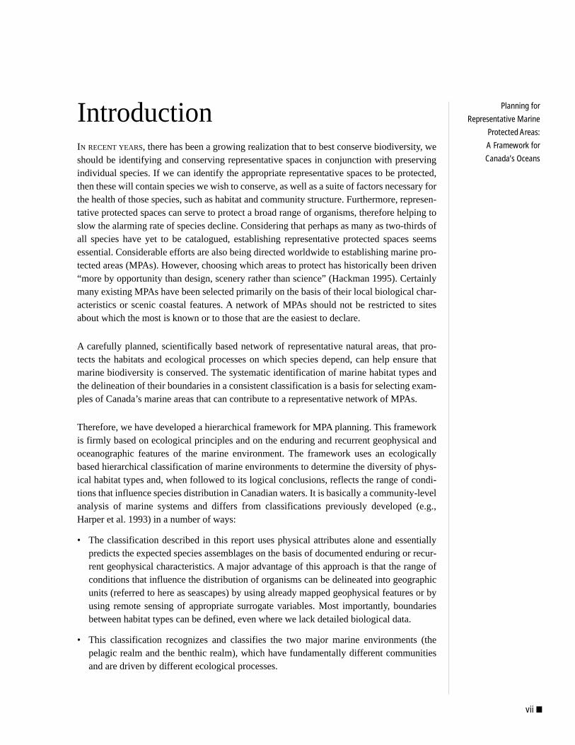
vii ■

Planning for

Representative Marine

Protected Areas:

A Framework for

Canada’s Oceans

IntroductionIN RECENT YEARS, there has been a growing realization that to best conserve biodiversity, weshould be identifying and conserving representative spaces in conjunction with preservingindividual species. If we can identify the appropriate representative spaces to be protected,then these will contain species we wish to conserve, as well as a suite of factors necessary forthe health of those species, such as habitat and community structure. Furthermore, represen-tative protected spaces can serve to protect a broad range of organisms, therefore helping toslow the alarming rate of species decline. Considering that perhaps as many as two-thirds ofall species have yet to be catalogued, establishing representative protected spaces seemsessential. Considerable efforts are also being directed worldwide to establishing marine pro-tected areas (MPAs). However, choosing which areas to protect has historically been driven“more by opportunity than design, scenery rather than science” (Hackman 1995). Certainlymany existing MPAs have been selected primarily on the basis of their local biological char-acteristics or scenic coastal features. A network of MPAs should not be restricted to sitesabout which the most is known or to those that are the easiest to declare.

A carefully planned, scientifically based network of representative natural areas, that pro-tects the habitats and ecological processes on which species depend, can help ensure thatmarine biodiversity is conserved. The systematic identification of marine habitat types andthe delineation of their boundaries in a consistent classification is a basis for selecting exam-ples of Canada’s marine areas that can contribute to a representative network of MPAs.

Therefore, we have developed a hierarchical framework for MPA planning. This frameworkis firmly based on ecological principles and on the enduring and recurrent geophysical andoceanographic features of the marine environment. The framework uses an ecologicallybased hierarchical classification of marine environments to determine the diversity of phys-ical habitat types and, when followed to its logical conclusions, reflects the range of condi-tions that influence species distribution in Canadian waters. It is basically a community-levelanalysis of marine systems and differs from classifications previously developed (e.g.,Harper et al. 1993) in a number of ways:

• The classification described in this report uses physical attributes alone and essentiallypredicts the expected species assemblages on the basis of documented enduring or recur-rent geophysical characteristics. A major advantage of this approach is that the range ofconditions that influence the distribution of organisms can be delineated into geographicunits (referred to here as seascapes) by using already mapped geophysical features or byusing remote sensing of appropriate surrogate variables. Most importantly, boundariesbetween habitat types can be defined, even where we lack detailed biological data.

• This classification recognizes and classifies the two major marine environments (thepelagic realm and the benthic realm), which have fundamentally different communitiesand are driven by different ecological processes.

■ viii

Planning for

Representative Marine

Protected Areas:

A Framework for

Canada’s Oceans

• By relying on enduring and recurrent geophysical features, this classification identifies“natural” habitat types even in areas heavily affected by human use. Biodiversity inthese highly disturbed areas might be impoverished or, at least, very different from thatwhich occurred previously, but could recover over time if the source of the distur-bances was removed.

The strengths of the framework are its abilities to do the following:

• Provide a defensible marine classification for Canada’s oceans based on a minimal setof key physiographic and oceanographic factors

• Systematically identify habitat types relating to marine communities and delineate theirboundaries in a consistent classification, ensuring that the full range of examplesdepicting Canada’s marine diversity are properly identified

• Provide a hierarchical system that both has a global perspective and considers the differences between benthic and pelagic systems, enabling the identification of variousfiner levels of seascapes down to the delineation of habitats

• Define a rational and attainable goal for a system of MPAs in Canada

• Provide a mechanism with which to evaluate and assess the contribution to the systemof all candidate MPAs, including those identified for reasons other than representation(e.g., unique features, endangered species habitat, fisheries management)

No other approach to marine classification systems provides all of these advantages. The framework proposed here should capture, in a network of systematically selectedMPAs, a greater level of biodiversity than other conservation approaches based solely on geography, indicator species, distinctive communities, and so on.

As a systematic and logical framework that all agencies and jurisdictions can use for theirown purposes, the framework has a variety of potential applications. It can be used as thefollowing:

• A common basis in the first step to determine representative MPAs or to assess MPAproposals from an ecological perspective

• A framework within which to plan and manage Canada’s marine environment

• A framework to monitor and report on the state of Canada’s network of MPAs

Similar frameworks for the hierarchical classification of all other aquatic habitats (estuar-ies, streams, rivers, lakes) could also be developed on the basis of the same fundamentalprinciples and similarly selected geophysical factors. This has not been done here becauseeach type of aquatic habitat would require a different array of factors in its own hierarchi-cal classification.

ix ■

Planning for

Representative Marine

Protected Areas:

A Framework for

Canada’s Oceans

The following arguments may be put forward against using this classification and theframework to determine a representative system of MPAs:

1. Why not just choose distinctive or special areas for MPAs? Such an approach wouldmean that MPAs would comprise only those communities about which we have someinformation. This approach ignores the importance of including representative areaswithin MPAs, and it also assumes that the important species and areas are the ones wecurrently know about.

2. There is not enough correlation between the biological communities and the physicalfactors. In this report, we advocate that the physical approach is essentially the onlypracticable approach in Canadian oceans where biological data are lacking over broadareas. A biological framework is not easily transportable to or reproducible acrossregions or coasts, and thus would not provide a consistent national framework for acountry such as Canada, with its vast coastline along three different oceans. However,wherever biological data do exist, this information should be used in conjunction withthe framework to optimize any decision making.

The framework was developed through the collaborative efforts of World Wildlife FundCanada and various academic and agency personnel.

This report is divided into four parts:

1. Part 1 is primarily about Canada’s marine biodiversity and the potential role of MPAsin conservation. Part 1 includes an outline of WWF Canada’s Endangered SpacesCampaign.

2. Part 2 compares physical and biological influences on marine ecosystems. It providesthe rationale and establishes the parameters for the physical approach to the frameworkoutlined in Part 3.

3. Part 3 outlines the general principles for designing a hierarchical framework and out-lines the proposed national framework for marine conservation, as well as the variousassumptions, limitations and caveats that also need to be considered.

4. Part 4 describes how the framework may be used to select and assess candidate MPAs.

Appendix 1 is a practical example of applying the classification framework developed inthis report to the Scotian Shelf on Canada’s east coast.

1Canada’s Marine Biodiversityand the Need for MarineProtected Areas

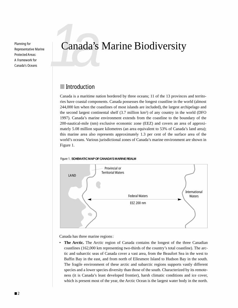
■ 2

Planning for

Representative Marine

Protected Areas:

A Framework for

Canada’s Oceans

■ IntroductionCanada is a maritime nation bordered by three oceans; 11 of the 13 provinces and territo-ries have coastal components. Canada possesses the longest coastline in the world (almost244,000 km when the coastlines of most islands are included), the largest archipelago andthe second largest continental shelf (3.7 million km2) of any country in the world (DFO1997). Canada’s marine environment extends from the coastline to the boundary of the200-nautical-mile (nm) exclusive economic zone (EEZ) and covers an area of approxi-mately 5.08 million square kilometres (an area equivalent to 53% of Canada’s land area);this marine area also represents approximately 1.3 per cent of the surface area of theworld’s oceans. Various jurisdictional zones of Canada’s marine environment are shown inFigure 1.

Figure 1. SCHEMATIC MAP OF CANADA’S MARINE REALM

Canada has three marine regions:

• The Arctic. The Arctic region of Canada contains the longest of the three Canadiancoastlines (162,000 km representing two-thirds of the country’s total coastline). The arc-tic and subarctic seas of Canada cover a vast area, from the Beaufort Sea in the west toBaffin Bay in the east, and from north of Ellesmere Island to Hudson Bay in the south.The fragile environment of these arctic and subarctic regions supports vastly differentspecies and a lower species diversity than those of the south. Characterized by its remote-ness (it is Canada’s least developed frontier), harsh climatic conditions and ice cover,which is present most of the year, the Arctic Ocean is the largest water body in the north.

1aCanada’s Marine Biodiversity

InternationalWatersFederal Waters

EEZ 200 nm

LAND

Provincial orTerritorial Waters

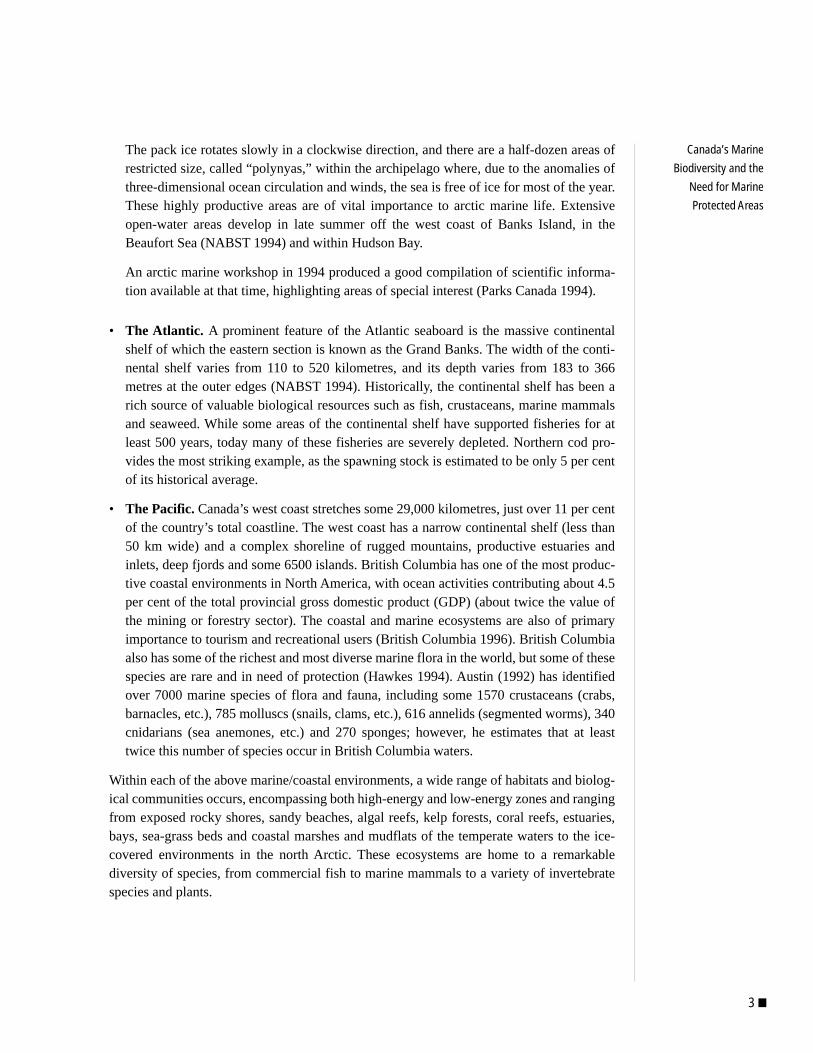
3 ■

Canada’s Marine

Biodiversity and the

Need for Marine

Protected Areas

The pack ice rotates slowly in a clockwise direction, and there are a half-dozen areas ofrestricted size, called “polynyas,” within the archipelago where, due to the anomalies ofthree-dimensional ocean circulation and winds, the sea is free of ice for most of the year.These highly productive areas are of vital importance to arctic marine life. Extensiveopen-water areas develop in late summer off the west coast of Banks Island, in theBeaufort Sea (NABST 1994) and within Hudson Bay.

An arctic marine workshop in 1994 produced a good compilation of scientific informa-tion available at that time, highlighting areas of special interest (Parks Canada 1994).

• The Atlantic. A prominent feature of the Atlantic seaboard is the massive continentalshelf of which the eastern section is known as the Grand Banks. The width of the conti-nental shelf varies from 110 to 520 kilometres, and its depth varies from 183 to 366metres at the outer edges (NABST 1994). Historically, the continental shelf has been arich source of valuable biological resources such as fish, crustaceans, marine mammalsand seaweed. While some areas of the continental shelf have supported fisheries for atleast 500 years, today many of these fisheries are severely depleted. Northern cod pro-vides the most striking example, as the spawning stock is estimated to be only 5 per centof its historical average.

• The Pacific. Canada’s west coast stretches some 29,000 kilometres, just over 11 per centof the country’s total coastline. The west coast has a narrow continental shelf (less than50 km wide) and a complex shoreline of rugged mountains, productive estuaries andinlets, deep fjords and some 6500 islands. British Columbia has one of the most produc-tive coastal environments in North America, with ocean activities contributing about 4.5per cent of the total provincial gross domestic product (GDP) (about twice the value ofthe mining or forestry sector). The coastal and marine ecosystems are also of primaryimportance to tourism and recreational users (British Columbia 1996). British Columbiaalso has some of the richest and most diverse marine flora in the world, but some of thesespecies are rare and in need of protection (Hawkes 1994). Austin (1992) has identifiedover 7000 marine species of flora and fauna, including some 1570 crustaceans (crabs,barnacles, etc.), 785 molluscs (snails, clams, etc.), 616 annelids (segmented worms), 340cnidarians (sea anemones, etc.) and 270 sponges; however, he estimates that at leasttwice this number of species occur in British Columbia waters.

Within each of the above marine/coastal environments, a wide range of habitats and biolog-ical communities occurs, encompassing both high-energy and low-energy zones and rangingfrom exposed rocky shores, sandy beaches, algal reefs, kelp forests, coral reefs, estuaries,bays, sea-grass beds and coastal marshes and mudflats of the temperate waters to the ice-covered environments in the north Arctic. These ecosystems are home to a remarkablediversity of species, from commercial fish to marine mammals to a variety of invertebratespecies and plants.

■ 4

Planning for

Representative Marine

Protected Areas:

A Framework for

Canada’s Oceans

The extent and diversity of Canada’s marine environments have resulted in some of themost spectacular marine life in the world: all major groups of marine organisms are repre-sented in Canadian waters, and many species are endemic or unique to them. For example,half the world’s population of narwhal, “the unicorn of the sea,” summers in Prince RegentInlet, Nunavut.

Approximately 1100 species of fish are recorded in Canadian waters (Ocean VoiceInternational 1996), and a wide variety of marine mammals occur, including beluga andnarwhal, and gray, bowhead, minke, humpback and killer whales, as well as sperm, north-ern bottlenose, blue and right whales farther offshore. Many other marine mammals such asdolphins, porpoises, seals, walruses, sea lions and sea otters can also be found in Canadianwaters.

The Committee on the Status of Endangered Wildlife in Canada (COSEWIC) lists over 50marine-associated species as extinct, endangered, threatened or vulnerable (COSEWIC1999). Species listed as endangered include the beluga and the bowhead and northern rightwhales. Threatened species include the harbour porpoise, sea otter, humpback whale andbeluga (eastern Hudson Bay population). Some marine mammal populations that wereonce exploited commercially and some that are traditionally used by Aboriginal people areexperiencing difficulty in recovering to viable or manageable levels. Some species wereaffected in the past by whaling or fur hunting; pollution, collisions with ships, fishing prac-tices and other human activities continue to affect them today. Many endangered andthreatened species in need of protection are key to ecosystem functioning and are also valu-able from an economic or a social perspective.

■ What Is Biological Diversity and Why Protect It?Biodiversity is, put simply, the richness and variety of life in the natural world. The inter-national Convention on Biological Diversity (UNEP 1994) defines biodiversity as “thevariability among living organisms from all sources, including ... terrestrial, marine andother aquatic ecosystems and the ecological complexes of which they are a part; thisincludes diversity within species, between species and of ecosystems.” The term “biodiver-sity” therefore encompasses genetic, species and ecological diversity, as well as the varietyof responses to environmental change.

The Convention on Biological Diversity refers to endangered species, threatened habitatsand ecosystem management in specific sections on the following:

• Conserving biodiversity by establishing protected areas (Article 8)

• Recovering endangered species and degraded ecosystems (Article 8)

• Protecting the traditional knowledge of Aboriginal people (Article 8)

• Integrating principles of sustainable use into decision making (Article 10)

• Applying economic and social incentives for conservation (Article 11)

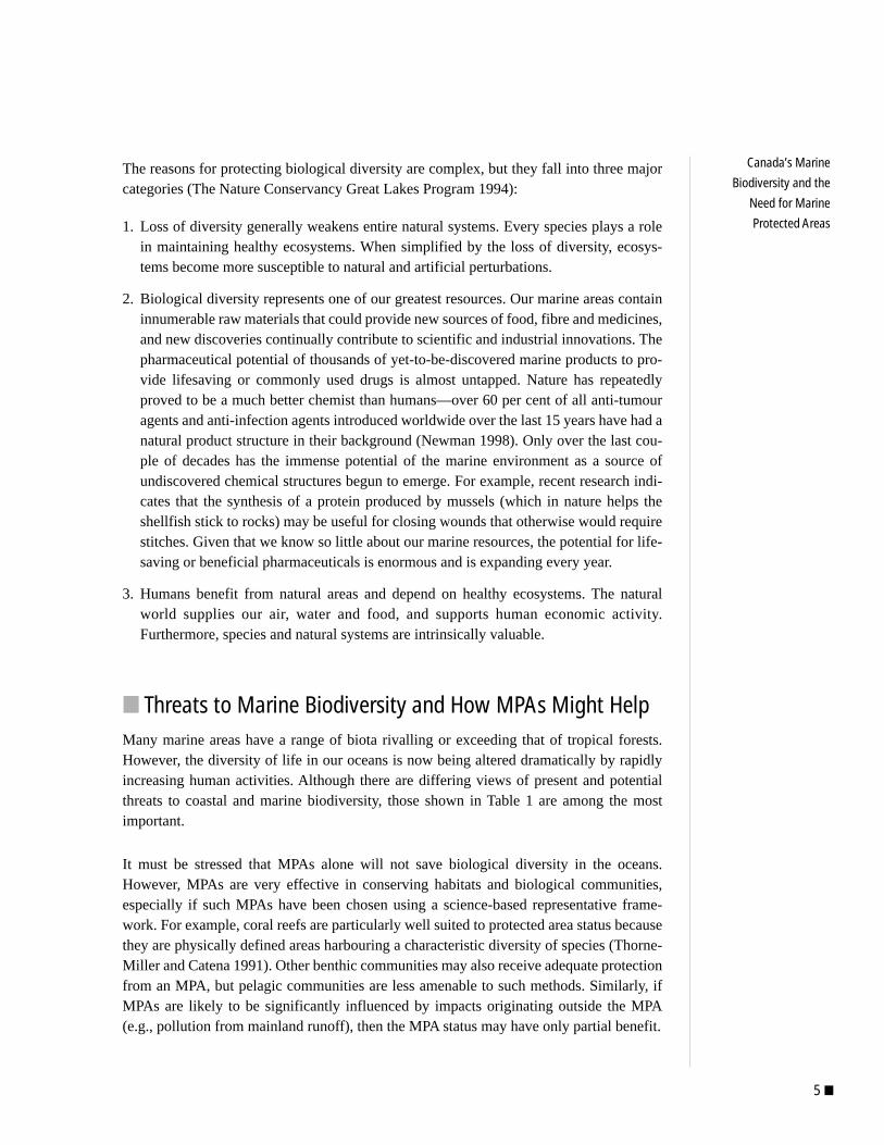
5 ■

Canada’s Marine

Biodiversity and the

Need for Marine

Protected Areas

The reasons for protecting biological diversity are complex, but they fall into three majorcategories (The Nature Conservancy Great Lakes Program 1994):

1. Loss of diversity generally weakens entire natural systems. Every species plays a rolein maintaining healthy ecosystems. When simplified by the loss of diversity, ecosys-tems become more susceptible to natural and artificial perturbations.

2. Biological diversity represents one of our greatest resources. Our marine areas containinnumerable raw materials that could provide new sources of food, fibre and medicines,and new discoveries continually contribute to scientific and industrial innovations. Thepharmaceutical potential of thousands of yet-to-be-discovered marine products to pro-vide lifesaving or commonly used drugs is almost untapped. Nature has repeatedlyproved to be a much better chemist than humans—over 60 per cent of all anti-tumouragents and anti-infection agents introduced worldwide over the last 15 years have had anatural product structure in their background (Newman 1998). Only over the last cou-ple of decades has the immense potential of the marine environment as a source ofundiscovered chemical structures begun to emerge. For example, recent research indi-cates that the synthesis of a protein produced by mussels (which in nature helps theshellfish stick to rocks) may be useful for closing wounds that otherwise would requirestitches. Given that we know so little about our marine resources, the potential for life-saving or beneficial pharmaceuticals is enormous and is expanding every year.

3. Humans benefit from natural areas and depend on healthy ecosystems. The naturalworld supplies our air, water and food, and supports human economic activity.Furthermore, species and natural systems are intrinsically valuable.

■ Threats to Marine Biodiversity and How MPAs Might HelpMany marine areas have a range of biota rivalling or exceeding that of tropical forests.However, the diversity of life in our oceans is now being altered dramatically by rapidlyincreasing human activities. Although there are differing views of present and potentialthreats to coastal and marine biodiversity, those shown in Table 1 are among the mostimportant.

It must be stressed that MPAs alone will not save biological diversity in the oceans.However, MPAs are very effective in conserving habitats and biological communities,especially if such MPAs have been chosen using a science-based representative frame-work. For example, coral reefs are particularly well suited to protected area status becausethey are physically defined areas harbouring a characteristic diversity of species (Thorne-Miller and Catena 1991). Other benthic communities may also receive adequate protectionfrom an MPA, but pelagic communities are less amenable to such methods. Similarly, ifMPAs are likely to be significantly influenced by impacts originating outside the MPA(e.g., pollution from mainland runoff), then the MPA status may have only partial benefit.

■ 6

Planning for

Representative Marine

Protected Areas:

A Framework for

Canada’s Oceans

Table 1. THREATS TO MARINE BIODIVERSITY

Risk or Speed Can the Risk to of Degradation Biodiversity Be of Biodiversity Threatening Process Reduced by an MPA?

High Physical habitat destruction (e.g., dredging) Yes

Blast fishing using explosives Yes

Toxic pollution (e.g., chemical spills) Maybe

Chemical fishing (e.g., using cyanide) Yes

Introduction of exotic organisms Maybe

Loss of genetic variability Yes

Biological invasions Maybe

Overexploitation/overfishing Yes

Bioaccumulation of noxious materials (e.g., heavy metals) Maybe

Indirect pollution (e.g., pesticides, herbicides in runoff) Maybe

Disease/parasite infection Maybe

Depletion of spawning sites Yes

Sea dumping of dredge spoil Yes

Incidental take/by-catch Yes

Destruction of adjoining watersheds Maybe

Impacts of adjacent land-use practices (e.g., aquaculture) Maybe

Effluent discharge (e.g., sewage, pulp/paper mill effluent) Maybe

Natural events (e.g., cyclones, tsunamis) No

Direct marine pollution, ocean dumping Yes

Downstream impacts from dams, dikes, etc. Maybe

Net/debris entanglement Maybe

Siltation Maybe

Noise pollution Maybe

Toxic blooms/red tides Maybe

Thermal pollution Yes

Rising sea temperatures (climatic change) No

Rising sea level (climatic change) No

Salinity changes No

Lowa Take by Aboriginal people Maybe

7 ■

Canada’s Marine

Biodiversity and the

Need for Marine

Protected Areas

a The high–low scale on the left side of this table is approximate; it seeks only to indicatethat some threatening processes have a higher risk and/or speed of degradation of marinebiodiversity than others. Moreover, the relative order of the various threatening processeson this scale is open to conjecture. However, it is important to note that MPAs are able toaddress only some of these issues.

The effectiveness of the protection afforded by an MPA to marine animals and plants thatoccur within it will therefore depend largely on these factors:

• The size of the area protected

• The activities that are restricted and allowed within the MPA boundaries

• The MPA designation and whether it restricts polluting activities that occur outside theMPA but that threaten life within the MPA

In protecting and conserving marine biodiversity, it is important to recognize that biodiver-sity can be understood, conserved and managed along a range of spatial and temporalscales. Biodiversity occurs at the scale of large marine ecosystems, such as major oceanicecosystems, and may be defined by broad-scale processes such as oceanography (i.e., cur-rents and upwellings) and trophodynamics, as well as coastal and oceanic physiographyand topography. Biodiversity also occurs at other scales, whether considered as communi-ties, habitats or specific sites. At these finer scales, patterns in biodiversity may be domi-nated by physical processes, such as cyclones, storm events, the tidal range, changes inwave exposure, and the type of substratum, or by biological processes, such as competitionand predation.

■ 8

Planning for

Representative Marine

Protected Areas:

A Framework for

Canada’s Oceans

■ Introduction to MPAsCompared to protected areas for terrestrial conservation and management, MPAs are arecent concept. Some countries had established MPAs prior to the first World Conferenceon National Parks in 1962, but this conference was probably the first time the need for pro-tection of coastal and marine areas was recognized internationally. However, the need for asystematic and representative approach to establishing protected areas in marine environ-ments was not articulated clearly until the International Conference on Marine Parks andProtected Areas, convened by the World Conservation Union (IUCN) in Tokyo in 1975(Kenchington 1996).

Today, there are over 1300 MPAs in more than 80 countries. These MPAs range in size fromseveral hundred square metres to 339,750 square kilometres (the largest being the GreatBarrier Reef Marine Park in Australia). This wide range of MPAs has been established for avariety of purposes:

• To preserve natural communities and free them from exploitation

• To help preserve important fisheries

• To protect historical and cultural resources

• To establish parks for diving

In Canada, there are approximately 155 protected areas with a marine component, 106 inBritish Columbia (MLSS nd) and 49 in the northwest Atlantic and Arctic areas (Kelleher etal. 1995). These MPAs may be designated as any of the following:

• National wildlife areas, declared under Canadian wildlife legislation

• Migratory bird sanctuaries, declared under Canadian wildlife legislation

• National parks and reserves, declared under national parks legislation

• National marine parks, declared under national parks legislation

• Provincial parks, declared under provincial legislation

1bMPAs and aRepresentative System

9 ■

Canada’s Marine

Biodiversity and the

Need for Marine

Protected Areas

Most of these MPAs have been established to conserve habitat for endangered species or toprotect significant features. However, it is not clear to what extent these MPAs contribute tothe protection of Canada’s marine diversity, as many are extremely small and offer littleprotection or limited enforcement. It is virtually impossible to determine their contributionto an overall system without an ecological context in which to assess them, that is, a repre-sentative framework that also considers the ecological processes that are essential to main-tain their long-term viability.

■ What Is a Representative System of MPAs?Hundreds of articles and texts have been written about MPAs throughout the world, andmany of these works refer to the importance of MPAs in representing marine biodiversityand preserving ecological processes. Few of these works, however, actually define a repre-sentative MPA system or provide a framework for determining how a representative systemshould be identified and how MPAs should be located to achieve ecological representationor to maximize marine biodiversity.

A representative system of MPAs is one that samples the full range of environmental gradi-ents, or habitat types, at a given scale. Declaring MPAs in the right place and of the rightsize and the right configuration will most efficiently complete a representative system andhelp protect biodiversity over the long term. The Canadian Environmental AdvisoryCouncil (1991) stated:

Priority must be placed on protecting representative natural areas. They are the corner-stone of a network of protected areas because of their significant contribution to con-serving biological diversity and sustaining ecological processes.

There needs to be a systematic, science-based framework within which to choose MPAsand assess progress toward a representative system. The purpose of this report is to devel-op a framework that provides the basis for mapping Canada’s oceans down to the level ofhabitat types, referred to here as seascapes. The representative system would be completeonce all the seascapes have been sampled, or captured within a set of MPAs.

However, MPAs chosen on a representative basis will not automatically include all theunique and special marine features we might want to protect. These features can be identi-fied and MPAs designed to incorporate them. In other words, not all MPAs need to beselected strictly by representation criteria. MPAs that are chosen to protect special marinefeatures can still contribute to completing a representative system provided that they meetecologically based protection criteria (e.g., size, level of protection, connectivity). Ananalysis of what these MPAs contribute to the representative system can be completed inhindsight. It must be said, however, that this approach will not achieve a complete repre-sentative system in the most efficient manner.

This part of the report describes in more detail the broader concept of MPAs declared for awide range of reasons and outlines the role of representation within this broader context. Aclear distinction between MPAs chosen for representation and those chosen for other valuesis important for a number of reasons:

1. While ecological representation is an important concept and is a sound basis upon whichto plan MPAs, not all government agencies with responsibility for MPAs have represen-tation as a mandate.1

2. The majority of existing MPAs in Canada, while providing varying degrees of ecologi-cal protection, nonetheless do contribute to marine conservation even if only by increas-ing public awareness.

3. Given the legislative mandate of those agencies that are able to declare reserves inmarine areas, it is important to understand how the determination of a representativeframework provides a systematic basis against which the role of existing MPAs may beassessed.

A representative approach to planning MPAs is not a new concept, but it has yet to be wide-ly accepted or implemented. Before explaining how the representative framework can beused to further the network of MPAs in Canada, it is important to first outline the broaderconcepts of MPAs as historically viewed and implemented by agencies.

■ The Broad Context of MPAsOne definition of an MPA that is commonly used throughout the world is that of the IUCN(Kelleher and Kenchington 1992):

[An MPA is] any area of intertidal or subtidal terrain, together with its overlying waterand associated flora, fauna, historical and cultural features, which has been reserved bylaw or other effective means to protect part or all of the enclosed environment.

Some users have found certain difficulties in applying this definition; for example,Nijkamp and Peet (1994) have these objections:

• The IUCN definition refers primarily to terrain rather than to marine waters, whichseems to emphasize the value of the seabed rather than the value of the overlying wateror associated flora and fauna.

• The reference to fauna and flora is too restrictive as it might exclude such marinefeatures as ocean vents, upwelling areas, and so on.

• An area that is reserved by law is not necessarily protected by law.

■ 10

Planning for

Representative Marine

Protected Areas:

A Framework for

Canada’s Oceans

1 Currently, the federal

government has three formal

programs for MPAs; these

programs have distinct but

complementary purposes and

are the responsibility of one

of the following agencies:

Parks Canada (Canadian

Heritage), Canadian Wildlife

Service (Environment

Canada), and Department of

Fisheries and Oceans (DFO).

11 ■

Canada’s Marine

Biodiversity and the

Need for Marine

Protected Areas

The AIDEnvironment study (Nijkamp and Peet 1994) therefore suggests a modified defin-ition of an MPA:

[An MPA is] any area of sea or ocean—where appropriate in combination with con-tiguous intertidal areas—together with associated natural and cultural features in thewater column, within, or on top of the seabed, for which measures have been taken forthe purpose of protecting part or all of the enclosed environment.

By either definition, a plethora of areas throughout the world could be termed MPAs.Ballantine (1991) cites some 40 names in common use around the globe for areas current-ly set aside for the protection of parts of the sea. He includes the following:

The varying definitions and multitude of labels may add to the debate by causing misun-derstanding and uncertainty. MPAs also range from small, highly protected “no-take”reserves that sustain species and maintain natural resources to very large, multiple-useareas in which the use and removal of resources is permitted but controlled to ensure thatconservation goals are achieved. The intention underlying the use of specific terminologymust be clarified.

■ DefinitionsFor the purposes of this report, let us assume a very basic and generic definition of anMPA:

An MPA is any marine area set aside under legislation to protect marine values.

Within this definition, the “marine values” may be virtually anything, including one ormore of the following:

• Marine park

• Marine reserve

• Marine nature reserve

• Marine habitat reserve

• Marine protected area

• National seashore

• Marine wildlife reserve

• Marine wilderness area

• Maritime park

• Marine sanctuary

• Marine life refuge

• Marine conservation area

• Conservation values

• Commercial values

• Enhancement of special species

• Scientific importance

• Historic features

• Recreational values

• Scenery/aesthetics

• Unique features

• Cultural values

• Traditional uses

■ 12

Planning for

Representative Marine

Protected Areas:

A Framework for

Canada’s Oceans

Given that many types of MPAs exist and that confusion has resulted from terminologybeing used in different ways in different documents, the terms used in this report aredefined as follows:

• A multiple-use MPA is an MPA in which the use and removal of resources may be per-mitted, but such use is controlled to ensure that long-term conservation goals are notcompromised. Multiple-use MPAs generally have a spectrum of zones within them, withsome zones allowing greater use and removal of resources than other zones (e.g., no-take zones are commonly designated as one of the zones of a multiple-use MPA).

• A no-take MPA is a special type of MPA (or a zone within a multiple-use MPA) where(a) any removal of marine species and modification or extraction of marine resources(by such means as fishing, trawling, dredging, mining, drilling) is prohibited, and (b)other human disturbance is restricted.

• A biosphere reserve is a protected area, generally large, that has highly protected coreareas surrounded by partially protected buffer areas and an outer transition zone. Boththe buffer zone and the outer zone may allow some ecologically sustainable use ofresources (e.g., low-impact use and traditional use) and also should have facilities forresearch and monitoring; such activities within these areas should not compromise theintegrity of the core area. The biosphere reserve concept was developed for terrestrialreserves but is considered by some2 also to have application for marine environmentsand hence MPAs (Price and Humphrey 1993).

As outlined below, MPAs may be created to preserve a wide range of values, and the goalor purpose of an MPA will influence the type of MPA and consequently its design andselection and, ultimately, its name.

■ What Are the Potential Benefits of MPAs?MPAs can provide a wide range of benefits, some of which are noted in Box 1.

Numerous publications have expanded on the wide range of benefits of MPAs; for exam-ple, at a workshop at the University of British Columbia in February 1997, the advantagesof no-take marine reserves were comprehensively discussed (Pitcher 1997). Box 2 summa-rizes the benefits that can reasonably be expected with an appropriate system of no-takemarine reserves (which should be accompanied by other marine management measures).3

These benefits can be grouped as follows:

1. Protection of ecosystem structure, function and integrity

2. Increased knowledge and understanding of marine systems

3. Improved nonconsumptive opportunities

4. Potential fishery benefits

2 Various authors (Batisse

1990; Kenchington and

Agardy 1990) suggest that

if the UNESCO Biosphere

Reserve Program were to be

redesigned and properly

planned and implemented, it

would provide a very useful

tool for the wider aspects of

marine conservation.

3 Adapted from a listing

produced by the Center for

Marine Conservation in

1995 (Sobel 1996).

13 ■

Canada’s Marine

Biodiversity and the

Need for Marine

Protected Areas

Box 1. POTENTIAL BENEFITS OF MPAs

• Protect many different kinds of habitat in all marine and aquatic regions of Canada.

• Protect critical habitat for rare and endangered species, such as the northern right whale and the beluga.

• Help protect key ecological functions and processes, such as upwellings, which are the “engines” ofmarine and freshwater systems.

• Serve as source or seed-bank locations for the production of eggs and larvae of commercial and recre-ational species, which may then move from MPAs to “seed” adjacent marine areas.

• Prevent overfishing by providing refuges to an intensely harvested species.

• Provide alternative and supplementary economic opportunities through such activities as whale watch-ing, scuba diving, boating, sightseeing and ecotourism.

• Serve as natural laboratories for the study of marine systems and as ecological benchmarks againstwhich human impacts and environmental trends can be monitored and measured.

• Serve as storehouses for currently undiscovered marine products that may one day lead to the discoveryand production of new food sources or lifesaving drugs.

• Lessen the effects of future management errors, accidents or unfavourable environmental changes, suchas changes in sea temperatures.

• Assist in the reestablishment of linkages between species that have been depleted or suppressed byexploitation (e.g., overfishing) and thus help reestablish, at least locally, ecological integrity.

• Fulfill Canada’s international obligations as a signatory to the Convention on Biological Diversity.

When the information shown in Box 2 was first developed by Sobel (1996), he qualified thebenefits of marine reserves with the following observations:

• The benefits grouped under ecosystem protection were among the most important andbest documented by the panel of experts.

• The priority placed on ecosystem protection reflects the view that ecosystem protectionis necessary, if not sufficient, to deliver the other listed benefits.

• Some categories overlap.

• Many benefits would accrue even from imperfectly designed marine reserves.

• The broad definition of ecosystem protection parallels the needs of biodiversity conser-vation as recognized elsewhere.

• Certain benefits to fisheries might be more sensitive to design but need additional test-ing in countries with a strong research capacity.

■ 14

Planning for

Representative Marine

Protected Areas:

A Framework for

Canada’s Oceans

Protection of Ecosystem Structure,Function and Integrity

• Protect the structure of physical habitat fromdamage by fishing gear and from other anthropogenic and incidental impacts.

• Maintain high-quality feeding areas for fish and wildlife.

• Protect biodiversity at all levels.

• Restore population size and age structure.

• Restore community composition (species presence and abundance).

• Promote ecosystem management.

• Protect the genetic composition of populationsfrom direct and indirect selection by fisheries.

• Encourage a holistic approach to management.

• Allow the distinction between natural and anthropogenic changes.

• Protect ecological processes, including keystonespecies, cascading effects, threshold effects,second order effects, food web and trophicstructure, and system resilience to stress.

Increased Knowledge and Understanding ofMarine Systems

• Provide long-term monitoring sites.

• Provide focus for study.

• Provide continuity of knowledge in undisturbed sites.

• Reduce risks to long-term experiments.

• Provide opportunity to restore ormaintain natural behaviour.

• Provide experimental sites that require natural areas.

• Provide natural reference areas for assessing anthropogenic effects (including fisheries).

Improved Nonconsumptive Opportunities

• Enhance and diversify economic opportunitiesand social activities.

• Provide wilderness opportunities.

• Enhance aesthetic experiences.

• Promote ecotourism.

• Enhance spiritual connection.

• Improve appreciation of conservation.

• Enhance educational opportunities.

• Enhance nonconsumptive recreation.

• Diversify the economy.

• Increase opportunities for sustainable employment.

• Create public awareness about the environment.

Potential Fisheries Benefits

• Increase abundance of overfished stocks withinthe reserve.

• Export juveniles, eggs or adults to fisheries outside of the reserve.

• Provide resource protection even when data arelacking.

• Provide undisturbed spawning habitats andconditions.

• Simplify enforcement and monitoring.

• Reduce by-catch mortality.

• Provide control areas for research on fisheries management.

• Reduce conflict within and between sectors.

• Restore natural community structure in thereserve (e.g., age structures and predator–preydistributions).

Box 2. EXPECTED BENEFITS OF AN APPROPRIATE SYSTEM OF NO-TAKE MARINE RESERVES

15 ■

Canada’s Marine

Biodiversity and the

Need for Marine

Protected Areas

■ How MPAs Can Benefit Endangered,Threatened or Rare SpeciesThe following sections on various aspects of conservation are adapted from a DFO discus-sion paper (1997), which outlines the conservation role of MPAs.

CONSERVATION OF KEYSTONE SPECIES

MPAs can assist in maintaining or reestablishing keystone species by protecting them fromactivities that affect their populations. The disappearance of a keystone species can alter ordisrupt the species structure and the functioning of an entire community, as occurred, forexample, following the exploitation of sea otters along the Pacific Coast. “As the popula-tions of sea otters declined because of trapping, their prey, the sea urchin, exploded in num-bers. Sea urchin food (kelp) disappeared, leaving ‘sea urchin barrens,’ a dramaticallydiminished habitat and a drastically changed community” (DFO 1997).

In this case, the damage was done before scientists and managers were aware of the key-stone role of the sea otter. Reintroduction of the sea otter by conservation agencies in recentdecades has reversed the ecological processes and led to a return of the kelp along withother algal species, crustaceans, squid, fish and other organisms (Wilson 1993). Remotenatural refuges offered protection that ensured the survival of the sea otter and provided theopportunity to reintroduce them to their former ranges.

CONSERVATION OF VALUABLE SPECIES

The DFO discussion paper (1997) notes the following:

Oceans contain innumerable raw materials that could provide new sources of food,fiber and medicines, and that could contribute to scientific and industrial innovations.… We cannot know in advance which species are likely to be important. For example,species such as sea urchins, sea cucumbers, rock crabs and Jonah crabs were oncethought to be of no commercial value, but have developed into locally significant fish-eries.

As has already been pointed out in this report, the pharmaceutical potential of our oceans isvirtually unknown, and only in recent decades has it begun to be explored.

CONSERVATION OF MARINE MAMMALS

Many marine mammals and their critical habitats can benefit from MPAs; consequently,such species and habitats are specifically identified in the Oceans Act as being worthy ofspecial protection through the establishment of MPAs. To limit the impact of detrimentalactivities, the “design of an MPA must consider the temporal and other special requirementsrelated to calving and feeding grounds, which can change over time. For example, highlymigratory species such as whales require national or even international networks of MPAsto protect them throughout their ranges” (DFO 1997).

■ 16

Planning for

Representative Marine

Protected Areas:

A Framework for

Canada’s Oceans

CONSERVATION OF UNIQUE HABITATS

MPAs designed to protect unique habitats have various benefits. “If a unique habitat has arare species which is endemic to an area, protection of that habitat is a means of preventingthe extinction of a species” (DFO 1997). For example,

some benthic communities are associated with specialized environments such ashydrothermal vents, isolated seamounts, and oceanic trenches or canyons. These unusualand isolated habitats result in confined ecological communities. The species endemic tothese habitats may be at risk because of their limited means of dispersing to recolonizeother areas. (DFO 1997)

Much remains to be learned about patterns of marine endemism; growing scientific evidenceindicates that many marine species are far less widely distributed than was previouslythought (Norse 1993). Many offshore benthic organisms, for example, are relatively restrict-ed in range.

Unique habitats can also be seen as having intrinsic value—that is, they are valuable becausethey are unique. Again, it is important to stress that a representative framework will not auto-matically include such unique or distinctive communities; these need to be identified sepa-rately to ensure they are protected in MPAs.

CONSERVATION OF BIODIVERSITY AND PRODUCTIVE ECOSYSTEMS

MPAs can provide an important tool for protecting marine biodiversity, as well as for main-taining productive marine ecosystems. Marine biodiversity can be adversely affected innumerous ways, including exploitation and overharvesting (particularly overfishing), physi-cal destruction of habitats, pollution, incidental take and the introduction of exotic organisms.

A number of highly productive ecosystems will benefit from the protection afforded by anMPA:

For example, many estuaries are highly productive, providing critical habitats for thelife stages of a variety of fish and other species. Estuaries are under considerable stressthroughout Canada, requiring greater levels of protection from both ocean and land-based activities. Similarly, upwelling and mixing areas typically have high productivityand support the life stages of a variety of fish, mammal, and other species. Upwellingoccurs under specific conditions in coastal locations, such as the west coast ofVancouver Island, in the St. Lawrence Estuary (at the mouth of the Saguenay River),and on the Atlantic offshore. Other highly productive and diverse ecosystems includeoffshore banks, kelp forests, and deep sea features such as sea vents. (DFO 1997)

Through strategic ecosystem-scale management and the judicial placement and man-agement of MPAs, the impacts of human use and activity can be regulated so that theydo not exceed the sustainable self-repair capacity of biodiversity and natural systems.

17 ■

Canada’s Marine

Biodiversity and the

Need for Marine

Protected Areas

However, to protect areas of high biodiversity and highly productive ecosystems, anMPA typically needs to be large—encompassing a variety of critical ecosystem compo-nents. This presents a unique management challenge, since it is often necessary to coor-dinate protection objectives with a variety of human activities. Consequently, the widevariety of factors and influences affecting productivity and biodiversity need to be con-sidered in the development of MPAs for this purpose. Often “no take” areas or zones arerequired in order to ensure that critical ecosystem functions and key species and com-munities are maintained. (DFO 1997)

CONSERVATION OF INTANGIBLE VALUES

Although intangible values are not quantifiable, many people believe that biodiversity hasintrinsic value and consider the loss of any species to be ethically unacceptable.

Studies show that, in considering habitat restoration, people place a higher value on theexistence of a species than on its potential for use (Vain and Bromley 1994). MPAs pro-vide an opportunity to protect species and habitats that are considered valuable fromthese perspectives. (DFO 1997)

■ Benefits of MPAs for Scientific Research4

The establishment of MPAs provides opportunities to achieve other benefits, including thoseresulting from marine scientific research. While such research may involve the testing ofmanagement approaches, the greatest value of research is in studying relatively untouchedmarine areas and in comparing them with others that have been subject to human use andactivities.

The Oceans Act (sections 35 and 42) enables the establishment of MPAs for marine scientif-ic research. Such research can

further our understanding of how ecosystems function and how conservation strategiescontribute to the recovery of marine species and communities.… Improved scientificknowledge will aid in coastal management and fisheries management. It can alsoaddress major gaps in our current understanding, reduce uncertainty, and provide a basisfor adaptive management and future planning. (DFO 1997)

■ Global Recognition of MPAsMPAs are now recognized internationally as being an essential and fundamental componentof marine conservation and are referred to within many international agreements, includingthe following:

• The United Nations Convention on the Law of the Sea (UNCLOS)

• The Convention on Biological Diversity and the accompanying Jakarta Mandate onMarine and Coastal Biological Diversity

4 Adapted from DFO 1997.

■ 18

Planning for

Representative Marine

Protected Areas:

A Framework for

Canada’s Oceans

• The Global Program of Action

• MARPOL 73/78 and the more recent International Maritime Organization (IMO) guide-lines

• The World Heritage Convention

■ Why Have So Few MPAs Been Declared in Canada?As Sobel (1996) states, “Despite overwhelming scientific evidence, empirical observationsand common sense, many people remain unconvinced or unaware that significant marinebiodiversity losses have already occurred, are continuing to occur and will continue tooccur.” There is, therefore, a real and urgent need to do something to remedy the paucity ofCanadian MPAs. Many reasons are given by those who oppose MPAs or by those who arecautious about the declaration of MPAs:

• There is no scientific proof that reserves work.

• MPAs may be effective elsewhere, but that doesn’t mean they will work here.

• The concept makes sense, but not enough information exists to properly design the perfect system.

• The resources aren’t really in trouble; it’s just a natural cycle.

• The resources are in trouble, but the problem is due to some other factor such as global warming or outside influences over which we have no control.

• The principle is good, but put them somewhere else (i.e.,“not in my backyard”).

• Fishing is already heavily regulated; the regulations just need time to work.

• It is not economically viable to reduce the area available for fishing.

There are encouraging signs that the federal government has recognized the need to declaresome MPAs quickly and at the same time is beginning to design a comprehensive plan for asystem of MPAs:

There is a balance to be sought between the need to act on critical areas immediatelyand the need to be systematic in looking at an overall MPA network. The judgment ofgovernment staff and users in discussions has been that we do not need to wait for fullnetwork systems plans to identify some of the known high priority areas. Indeed, wait-ing for such plans can delay overdue action. Typically, certain important areas are des-ignated in advance of a systems plan. The best approach is to begin consideration of pri-ority areas while at the same time proceeding on a systematic basis, conductingoverviews of marine regions to identify candidate MPAs. (DFO 1997)

19 ■

Canada’s Marine

Biodiversity and the

Need for Marine

Protected Areas

■ How Many Benefits Can a Representative System of MPAs Provide?It is clear that MPAs provide a wide range of benefits, all of which are important for marineconservation. The extent to which an MPA offers benefits in addition to its contribution torepresentation (i.e., which seascapes it has sampled) will depend on the size and location ofthe MPA and various other factors. A carefully planned, scientific analysis of seascapes is asound basis for conserving marine biodiversity for the following reasons:

• The systematic identification of marine habitats and the delineation of their boundariesin a consistent classification can ensure that the full range of Canada’s marine habitattypes are properly identified and can be protected, not just those areas about which weknow the most.

• A representative system of MPAs can help ensure that all the essential elements ofmarine community diversity in Canada are secured by protecting a sample of all thehabitats and the ecological processes on which species depend. This is something that noother approach to determining MPAs can ensure.

There are three essential steps in completing a national system of MPAs that will mosteffectively conserve marine biodiversity:

1. There must be a rational approach to determining ecological representation. The purposeof this report is to provide the framework necessary for this first step.

2. There must be a method to systematically choose a network of candidate MPAs thatsamples all habitat types identified in step 1.

3. There must be further assessment of candidate MPAs to ensure, wherever possible, thatother important, unique or distinctive ecological features are incorporated. Candidatesites must also be further assessed using other non-ecological criteria (e.g., economic,political, social, legal or pragmatic reasons). If, for valid reasons, the candidate MPAsinitially chosen are deemed inappropriate, then other candidate MPAs are similarlyassessed, leading to finalization of acceptable MPAs and ultimately to a representativenetwork of MPAs.

■ 20

Planning for

Representative Marine

Protected Areas:

A Framework for

Canada’s Oceans 1cCanada’s Biodiversity Strategyand the Role of MPAs

■ IntroductionLarge areas of the world’s coastal and marine environment are under considerable ecologi-cal stress due to a number of threats, the most significant being pollution, overfishing andhabitat destruction resulting from the physical alteration of the seabed or the coastline(Kelleher 1994). More pollution, including agricultural runoff, sewage, sediments fromconstruction and deforestation, and airborne emissions, enters marine waters from land-based activities than from any other source (World Resources Institute 1994).

■ Canada’s Biodiversity StrategyMathews-Amos (1997) describes the status of marine conservation:

Clearly something needs to be done because current efforts at protecting biologicaldiversity—both marine and terrestrial—are not enough. Marine conservation biologyefforts are at least two decades behind terrestrial efforts, but, like a mythical sea mon-ster emerging from the deep ocean, the mysterious marine problems now showing theirfaces are too alarming for scientists and policy makers to ignore any longer.

Canada’s response to the international Convention on Biological Diversity was the develop-ment of a national strategy—the Canadian Biodiversity Strategy—which has six goals (Env-ironment Canada 1995). The six goals of the Canadian strategy are as follows:

1. Conserve biodiversity by

• maintaining populations of native flora and fauna in their functioning ecosystems;

• establishing and managing protected areas;

• using biological resources and ecosystems sustainably.

2. Improve understanding of ecosystems and increase capability to manage resources by

• undertaking appropriate research and using traditional knowledge;

• undertaking integrated planning and ecological management;

• improving information and data management systems and monitoring.

3. Promote conservation and sustainable use.

4. Maintain or develop incentives and legislation to achieve conservation.

5. Cooperate with global partners in conservation.

6. Assist Aboriginal communities in implementing the biodiversity strategy.

21 ■

Canada’s Marine

Biodiversity and the

Need for Marine

Protected Areas

■ The Role of MPAs While MPAs might provide protection for valuable features in specific areas, the tradition-al approach for MPAs usually meant that the surrounding and connecting seas andupstream land areas remained subject to resource extraction, harvesting and managementby other resource agencies or, in some cases, subject to no management at all. Thorne-Miller and Catena (1991) suggest five requirements for the effective protection of marinebiological diversity:

• Regulation of land-based and maritime sources of pollution

• Coastal zone management

• Direct regulation of marine resources

• Establishment of MPAs

• Use of economic incentives and disincentives

These five requirements are discussed below.

1. Regulation of land-based and maritime sources of pollution. While this requirementdoes not provide for direct protection of species, it attacks the single greatest threat tomarine species and marine ecosystems, particularly pollution that causes long-termdamage. By far the greatest source of pollution of the sea is land-based human activity;mainland environmental problems are usually reflected in marine problems (e.g., soilerosion results in suspended particles, often with nutrients attached as ions, being con-veyed to the sea).

As well, spills of hazardous materials such as oil are a continuing threat. No country inthe world has the capacity to combat a major oil spill adequately. While avoiding spillsis far more important than preparing for their cleanup, such spills are inevitable, so ade-quate preparation for dealing with them is crucial.

2. Coastal zone management. This requirement recognizes the interrelated functions ofthe coastal zone and the need to avoid segregated “sector” management, which regulatesparticular activities without taking into account other activities affecting the sameresources. Since it is not always possible to set aside totally protected areas, integratedcoastal management is becoming increasingly accepted as the most effective means ofdealing with such complex issues and areas.

3. Direct regulation of marine resources. The regulation of fisheries and other harvestingactivities in the oceans is becoming increasingly critical as overfishing by commercialand recreational interests becomes more prevalent. Virtually every international marinefishery is considered by most experts to be inadequately managed for ecological sus-tainability (Kelleher 1994). Regulations need to cover more than just catch limits on tar-get species; regulations regarding nontarget species (or by-catch)—including fishspecies, marine mammals and turtles—are necessary. In addition, a range of other fish-ery management techniques (e.g., species quotas; gear restrictions; and regulation oftimes, areas and numbers of licences) should be applied.

■ 22

Planning for

Representative Marine

Protected Areas:

A Framework for

Canada’s Oceans

4. Establishment of MPAs. MPAs will make a key contribution to the long-term viabilityand maintenance of marine ecosystems if the network of MPAs has a representativebasis and if the MPAs are adequate in size and connectivity. However, as outlinedabove, MPAs should be regarded as only part of integrated marine or coastal manage-ment. MPAs should exist within the context of large sustainable-use management areas,rather than as isolated, highly protected enclaves within heavily used areas.

5. Use of economic incentives and disincentives. Frequently, both regulatory and man-agement approaches fail to maintain the necessary level of biological diversity. Untilrecently, governments have used economic incentives to encourage the exploitation ofnatural resources, often well beyond their natural capacity to replenish themselves.Those economic policies can be altered so that the sustainable use of resources becomesthe guiding principle for economic incentives. McNeely (1988) and Thorne-Miller andCatena (1991) both suggest such methods at the community, national and internationallevels.

The Oceans Management Strategy (OMS), Part II of Canada’s Oceans Act, identifies threecomplementary initiatives that will be part of a national strategy for managing Canada’soceans. These legislated initiatives include MPAs; integrated management of activities inestuaries, coastal waters and marine waters; and marine environmental quality. The OMSwill provide the basis for incorporating MPAs into a broader national planning frameworkfor the coastal zone. At the same time, stakeholders will participate in developing the over-all vision of MPAs for Canada.

The Oceans Act also states that the national strategy will be based on the principles of sus-tainable development, integrated management and precautionary approaches. Consequent-ly, the application of these principles will be an integral part of developing and implement-ing the MPA program.

In recent years there has been increased focus on defining goals and principles for the management of natural systems (e.g., Agee and Johnson 1998; Kessler et al. 1992; Norton1992; Grumbine 1994). Edyvane (1996) identifies several dominant themes that must beunderstood before natural systems can be managed:

• The hierarchical nature or structure of ecosystems (i.e., the need to adopt a systemsperspective)

• The definition of ecological boundaries (which inevitably do not correspond to artifi-cially determined administrative or political boundaries)

• The maintenance of ecological integrity (protecting biodiversity, patterns and process-es; maintaining viable populations and natural disturbance regimes; and facilitatingspecies reintroductions)

• The importance of data collection, monitoring and adaptive management

• The need for interdisciplinary research (e.g., bioeconomic analysis)

• The importance of scenario modelling and decision support systems

23 ■

Canada’s Marine

Biodiversity and the

Need for Marine

Protected Areas

• The role of spatial modelling and geographic information systems

• The need for interagency cooperation and organizational change

• The need to investigate human effects on ecosystem structure and function

• The importance of human social values

MPAs are an integral and critical component of the management of coastal and marineresources. To achieve a viable system of MPAs, however, the effects of surrounding marineand terrestrial areas must be recognized and managed. Therefore, the quality, quantity andaccessibility of ecological data and human-use information available to decision makersmust be improved.

1d

■ 24

Planning for

Representative Marine

Protected Areas:

A Framework for

Canada’s Oceans

WWF Canada’s EndangeredSpaces Campaign

The goal of WWF Canada’s Endangered Spaces Campaign has been the completion of anational network of protected areas that will adequately represent all of Canada’s terrestrialnatural regions by the year 2000, and marine natural regions (including the Great Lakes) bythe year 2010. The importance of completing such a representative network of protectedareas has won international acceptance in conservation planning fora. Furthermore, theConvention on Biological Diversity commits Canada to establishing a system of protectedareas.

Underlying the WWF Canada goal is the belief that conservation of biodiversity will not beachievable without a well-planned, science-based system of properly protected areas.

As in the methodology for identifying terrestrial protected areas published by WWF Canadain 1995, the methodology for identifying representative areas in marine systems should bebased on ecological principles and should identify a distinct goal. It is important to remem-ber that the focus of the WWF Canada campaign is on ecological representation rather thanon protecting some arbitrary percentage of the country’s marine areas.

WWF Canada’s objectives for this report are to do the following:

• Develop a nationally consistent framework for the planning and establishment of anationwide system of ecologically representative MPAs to ensure that they addressmarine representation within Canada’s three oceans.

• Increase awareness among relevant governments, agencies, interest groups and theCanadian public regarding the objectives of and needs for developing a representativenetwork of MPAs.

WWF Canada has the view that, in terms of the level of environmental protection theyafford, many MPAs currently existing in Canada are inadequate due to the types of activitiesthat may be allowed within them (that is, the existing legislation does not prohibit certainactivities considered incompatible with the goals of an MPA). For this reason, WWF Canadahas determined the minimum protection standard it considers necessary for an area to bedeemed an effective MPA. This standard is described in Box 3.

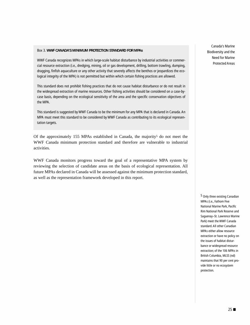
25 ■

Canada’s Marine

Biodiversity and the

Need for Marine

Protected Areas

Of the approximately 155 MPAs established in Canada, the majority5 do not meet theWWF Canada minimum protection standard and therefore are vulnerable to industrialactivities.

WWF Canada monitors progress toward the goal of a representative MPA system byreviewing the selection of candidate areas on the basis of ecological representation. Allfuture MPAs declared in Canada will be assessed against the minimum protection standard,as well as the representation framework developed in this report.

Box 3. WWF CANADA’S MINIMUM PROTECTION STANDARD FOR MPAs

WWF Canada recognizes MPAs in which large-scale habitat disturbance by industrial activities or commer-cial resource extraction (i.e., dredging, mining, oil or gas development, drilling, bottom trawling, dumping,dragging, finfish aquaculture or any other activity that severely affects the benthos or jeopardizes the eco-logical integrity of the MPA) is not permitted but within which certain fishing practices are allowed.

This standard does not prohibit fishing practices that do not cause habitat disturbance or do not result inthe widespread extraction of marine resources. Other fishing activities should be considered on a case-by-case basis, depending on the ecological sensitivity of the area and the specific conservation objectives ofthe MPA.

This standard is suggested by WWF Canada to be the minimum for any MPA that is declared in Canada. AnMPA must meet this standard to be considered by WWF Canada as contributing to its ecological represen-tation targets.

5 Only three existing Canadian

MPAs (i.e., Fathom Five

National Marine Park, Pacific

Rim National Park Reserve and

Saguenay–St. Lawrence Marine

Park) meet the WWF Canada

standard. All other Canadian

MPAs either allow resource

extraction or have no policy on

the issues of habitat distur-

bance or widespread resource

extraction; of the 106 MPAs in

British Columbia, MLSS (nd)

maintains that 90 per cent pro-

vide little or no ecosystem

protection.

2Marine Science and Ecosystems

2a

■ 28

Planning for

Representative Marine

Protected Areas:

A Framework for

Canada’s Oceans

Comparison Between Marineand Terrestrial Ecosystems

■ IntroductionOf all the species known to science, about 80 per cent are terrestrial, but there are moreorders and phyla in the sea. In fact, all phyla of animals are found in the sea, a majorityof these in benthic environments, and one third of the phyla are exclusively marine. Ifplants and protista [bacteria, fungi, algae and protozoa] are also considered, at least 80per cent of all phyla include marine species. In addition, the relative abundance ofmarine species may be greater, since most marine species are unknown. (Thorne-Millerand Catena 1991)

For marine conservation to be successful, the similarities and differences between marineand terrestrial ecosystems need to be understood. Any attempt to protect marine biodiversi-ty simply by applying terrestrial conservation methods will encounter difficulties. Marineecosystems are more connected than terrestrial ecosystems, and therefore physical influ-ences tend to propagate over a broader area and over longer periods of time. Unlike in ter-restrial ecosystems, the fundamental attributes, biological characteristics and even thespecies of marine ecosystems are not directly observable.

■ Similarities Between Terrestrial and Marine EcosystemsAt a very broad conceptual level, marine and terrestrial ecosystems have many similarities:

• Both are composed of interacting physical and biological components, with energyfrom the sun driving most systems.

• Both are complex patchworks of differing environments that are occupied by differentcommunities and species.

• Both marine and terrestrial species show a gradient in diversity with latitude—that is,species diversity generally increases with decreasing latitude (Thorne-Miller andCatena 1991).

• In both ecosystems, the primary zones of biological activity tend to be concentratednearer the surface (i.e., the land–air and the sea–air interface).

29 ■

Marine Science

and Ecosystems■ Differences Between Terrestrial and Marine EcosystemsMany differences exist between marine and terrestrial ecosystems. These differences can befound in such variables as space and time scales of physical processes; mobile versus sessilelife styles; and size, growth rate and factors relating to trophic position (Steele et al. 1993;Steele 1995). Differences are also related to the fundamental physical properties of wateritself (e.g., Sverdrup et al. 1942).

PHYSICAL AND BIOLOGICAL DIFFERENCES

Size: The combined seas are far larger in area than the combined land masses. The PacificOcean alone could easily contain all the continents. Even more important is the difference involume between marine and terrestrial habitats. Life on land extends roughly from the topsof trees to a few metres below ground—a vertical extent of about 30 to 40 metres. Althoughbirds, bats, arthropods and bacteria may periodically rise above these heights, the areaabove the treetops is more properly seen as one suited to temporary dispersal, rather than asan essential habitat, since species must return to the ground or trees for resources, reproduc-tion and shelter. The average depth of the oceans is 3800 metres, all of it containing livingcreatures. The sea’s habitable volume is therefore hundreds of times greater than that of theland.

Viscosity and density: Terrestrial and marine ecosystems differ markedly in their physicalproperties. For example, the water overlying the seabed is 60 times more viscous than airand has greater surface tension than the air overlying the land. Water is also about 850 timesdenser than air; this property provides buoyancy, allowing organisms, many of them verydifferent from organisms existing on land, to survive without the need for powerful sup-porting structures. Seawater’s buoyancy and viscosity keep food particles suspended andresult in an environment—the pelagic realm—without analogue in the terrestrial environ-ment. Specialized subcomponents of this realm, just beneath or at the sea–air interface, arethe plueston and neuston.

Temperature: The strong seasonal and long-term temperature fluctuations in the terrestrialclimate contrast with the moderate temperature fluctuations in the marine environment.Seawater has a much greater heat capacity than air, therefore temperatures change moreslowly in the sea than they do on land. The higher viscosity of seawater makes it circulatemore slowly than air.

Benthic and pelagic realms: The oceans contain two distinct realms, each with its owncommunities: the pelagic realm (the water column from the surface to the bottom) and thebenthic realm (the seabed and the layer of water immediately above it). Even within thepelagic realm, conditions vary dramatically with depth, which affects community structure.For example, due to changes in pressure and available light and nutrients, the communitiesinhabiting the top 20 metres of the ocean are very different from communities 1000 metresbelow the surface. The benthic realm can be compared to terrestrial ecosystems, wherespecies either live on the ground (or seabed) or are dependent on it for habitat and resources.

■ 30

Planning for

Representative Marine

Protected Areas:

A Framework for

Canada’s Oceans

However, a significant difference between the benthic realm and terrestrial ecosystems isthat most of the benthic realm is below the photic zone, that is, below the depth whereenough light penetrates for photosynthesis to occur. Therefore, unlike in most terrestrialecosystems, most of the benthic community does not have primary producers but must relyon resources that settle from the upper pelagic zone. The pelagic realm has no counterpartin terrestrial ecosystems as there are no terrestrial species (let alone whole communities)that are completely independent of the ground or ground-based resources.

Mobility and fluidity: The fluid nature of the marine environment means that many marinespecies are widely dispersed, and individuals can be far ranging. In addition to enhancingcross-fertilization and dispersal, water motion also enhances the migration and aggregationof marine species (especially those in pelagic systems). Water also dissolves and circulatesnutrients (Denman and Powell 1984; Mackas et al. 1985; Thorne-Miller and Catena 1991).Even marine species that can be considered static as mature forms (e.g., many molluscs andseaweeds) usually have highly mobile larval or dispersive reproductive phases, and theirpopulations may be controlled by mobile predators. This means that it may be extremelydifficult for such species to be managed as spatially defined populations. Similarly, the sed-iments of the substrate are themselves often so mobile that land erosion cycles seem slowand mild in comparison (Ballantine 1991).

Circulation: Although both terrestrial and aquatic environments exhibit patterns of circula-tion, that is, circulation of the water in the oceans and of the atmosphere above land andwater, the two are not strictly comparable. In the oceans, the medium—water—contains theorganisms themselves; aquatic organisms live in the medium, flow with it and are dominat-ed by it. In contrast, the presence of organisms in the atmosphere is strictly temporary.Thus, in the ocean, recruitment failure in one region may be reversed by passive recruit-ment from another area. On land, a similar process generally requires active migration(National Research Council 1994). Even for benthic communities, movements of the over-lying waters are essential for the transport of food resources; the atmosphere does not fulfilla similar function for terrestrial communities.

Light: Compared to the terrestrial realm, a far greater portion of the marine realm does notreceive light. Light is necessary for primary production through photosynthesis, except athydrothermal vents, which are dependent on their own chemosynthetic producers.Therefore, essentially no organic matter is produced in the vast, unlit depths of the ocean(the dysphotic and aphotic zones), and species in these dark areas must depend on the fluxof organic matter from the productive surface layer.

Primary production: The most obvious biological difference between terrestrial andmarine ecosystems may be in the types and source of primary production (Steele 1991b). Interrestrial ecosystems, primary producers (mainly vascular plants such as trees and grass)constitute the great majority of biomass, and individuals are often large. In contrast, thedominant primary producers in marine ecosystems—the phytoplankton—are generallymicroscopic and can reproduce rapidly. Consequently, they have much higher turnoverrates compared to the forests or prairies of terrestrial ecosystems.

31 ■

Marine Science

and Ecosystems

In terrestrial ecosystems, the biomass of primary producers tends to be highly conserved (e.g.,in woody plants). In contrast, in marine ecosystems the biomass of primary producers israpidly processed, either by consumers or reducers. Therefore, marine sediments are typical-ly much lower in organic carbon than terrestrial soils and become progressively lower stillwith increasing depth. Even marine macrophytic plants (e.g., algae and sea-grass angio-sperms), though often perennial, have short generation times compared to terrestrial plants.No marine plants have the longevity of terrestrial gymnosperms and angiosperms. At lowerlatitudes, the partially seawater-adapted mangroves (emergents) are recent reinvaders ofmarine waters.

Ecological response to environmental change: Other important differences between terres-trial and marine ecosystems result from—or are associated with—the temporal and spatialscales of ecological response to changes in the physical environment (Steele 1974, 1985,1991a, 1991b; Parsons 1991; Longhurst 1981; Cole et al. 1989) and are related to the funda-mental differences in the communities of primary producers and to the properties of water.The high storage of biomass in terrestrial organisms and organic detritus tends to decouplebiological and physical processes to some degree. In the oceans, however, the space and timescales of physical and biological processes are nearly coincident; biological communities canrespond rapidly to physical processes. Spatial variation and distribution of primary producerson land are largely related to topography and soil; such processes occur more slowly on landthan in marine ecosystems. On land, largely as a function of the longer generation times oflarger organisms, population and community cycles may depend more on biological than onimmediate physical processes (Steele et al. 1993). However, at all spatial scales, physicalchanges in the atmosphere are faster than in the ocean. Cyclonic systems in the atmospherehave typical diameters of about 1000 kilometres and last for about a week. Equivalent eddiesin the ocean have diameters of about 100 kilometres and can last for months or years (Steele1995). Thus we have the apparent paradox of “slowly responding” terrestrial communitiesbuffeted by a faster moving atmosphere, while in the oceans we have “quickly responding”communities within a slowly reacting and insulating ocean!

Bedrock type: Unlike in terrestrial ecosystems, bedrock type and geological compositionapparently have little influence on the biota of the marine benthos. This is at least partially afunction of the global constancy of the composition of seawater. Within the intertidal and sub-tidal euphotic zone, macrophytic algae are attached to rocks of all types. Within these samezones where soft substrates exist, it is tidal velocity and wave motion that determine substrategrain size and together they become the main determinants of community composition.

Ecological boundaries: Terrestrial environments have more pronounced physical boundariesbetween ecosystems. Especially at finer scales, it may be difficult to identify distinct bound-aries between marine ecosystems because they are so dynamic and because pelagic and ben-thic realms require separate consideration. This does not mean there are no distinct marineecosystems, but generally the boundaries are more transitional. Nevertheless, it is still appro-priate to examine the broad marine ecological characteristics and to define representativehabitat types in terms of their related enduring geophysical factors or recurrent processes.

■ 32

Planning for

Representative Marine

Protected Areas:

A Framework for

Canada’s Oceans

Longitudinal diversity gradients: In addition to the latitudinal gradients observed in bothterrestrial and marine environments, a longitudinal diversity gradient exists in the marineenvironment, decreasing from west to east in both the Atlantic and Pacific Oceans. As well,fauna in the Pacific Ocean (e.g., coral reefs) are more diverse on the whole than in theAtlantic Ocean (Thorne-Miller and Catena 1991). The greater diversity in the western partof these oceans can be related to the eccentric circulation pattern within them, whereby thewestern part receives water from low latitudes (with higher species diversity) at high veloc-ity (e.g., the Gulf Stream in the Atlantic Ocean and the Kuroshio, or Japanese Current, inthe Pacific Ocean), while the eastern part receives water at lower velocity from higher lati-tudes (with lower species diversity). The greater overall species diversity of the PacificOcean is generally explained in terms of its greater geological age.

Faunal diversity at higher taxonomic levels: At higher taxonomic levels, the diversity ofmarine fauna is much greater than the diversity of terrestrial fauna (Ray and McCormick-Ray 1992); all phyla of animals are represented in the oceans. Some taxa, for example, thefishes, are extraordinarily diverse; others are less diverse, although in “lower” phylaundoubtedly many species remain to be described.

Life span and body size: In the open ocean, there is a regular increase in life span and inbody size with increasing trophic level (Sheldon et al. 1972), whereas in terrestrial systemsthese patterns are not so clear (Steele 1991b).

■ Human Perspectives and ConsiderationsObservability of marine ecosystems: A very basic difference between marine and terres-trial ecosystems is that most of the marine environment is hidden from human sight, result-ing in major differences in our knowledge and understanding of these ecosystems. Our “outof sight, out of mind” mentality and the vastness of our oceans have both contributed to themisguided belief that the oceans can harmlessly absorb whatever we drop into them.Similarly, because the sea is remote and is an alien environment, demonstrating the needfor marine protection has been difficult. The collapse of commercial fisheries in many areasof the world has begun to raise awareness of the need for marine conservation.

Difficulties of marine research: Research and monitoring are far more difficult in andunder the water than they are on land. The exponential increase in the cost of obtaining datafrom increasing water depths explains why so little is known about the sea, especially thedeep oceans. The difficulty and expense of maintaining even moderately stable workingconditions at sea are so great that most marine research and management is virtually “hitand run,” after which the researchers and managers come home to land. Furthermore, farfewer people are employed to investigate or manage marine ecosystems, yet the marineareas to be investigated and administered are far greater than terrestrial areas.

33 ■

Marine Science

and Ecosystems

Known extinction rates: While current estimates of species loss in terrestrial ecosystemsare frightening, because of the lack of study little is known about, or even predicted for,species extinctions in marine ecosystems. Canada is not without examples, though, whichinclude the extinction of the great auk, Labrador duck and eelgrass limpet and, more recent-ly, the near disappearance of the barndoor skate. Recent evidence shows that many marinespecies worldwide are in dire straits, especially those with commercial value (e.g., whales,sea turtles, dugongs and many fish species).

Ownership: Until very recently, it was commonly accepted that no one owned a piece of thesea or any of its resources (this is now changing following successful sea claims byAboriginal people). Certainly in the more developed countries, it has long been felt, andgenerally still is, that marine resources were there for the taking or using by anyone who hadthe skill and initiative to do so (Ballantine 1991). Today, governments are taking on specificresponsibilities for some marine areas, but unfortunately most marine environments remainsubject to the “tragedy of the commons.” Responsibility for international waters is ham-pered by the mobility of water masses and connectedness of oceanic and territorial seas.

Resource extraction: During terrestrial resource extraction, the physical landscape is oftenaltered dramatically and visibly. It has recently been realized that the harvesting of marineresources can also dramatically alter the sea floor on a large scale. Much of the floor of theNorth Sea, for example, resembles a plowed field due to trawling activities. Marine conser-vation requires regulation of all types of resource extraction, including those that directlydisrupt the physical seascape (e.g., oil drilling and mining), and activities, such as commer-cial harvesting (e.g., bottom dredging, bottom trawling and dragging) and aquaculture thatperturb the sea floor at smaller scales but over broad areas.

Delineating park boundaries: On land, it is easy to mark park boundaries using signs ornatural features. At sea, the absence of obvious geographical features makes it difficult formarine users to determine if they are inside a protected area and when to curtail their har-vesting activities. However, it is hoped that the increasingly common use of global position-ing systems (GPS) makes this a diminishing concern.

■ Biogeochemical LinkagesThe sea is biogeochemically “downstream” from the land; thus virtually any substancereleased into the ecosphere is carried seaward. This has obvious implications for marine pol-lution as many inputs into marine systems have terrestrial origins.

The natural hydrological cycle flows from the land to the sea. Water is returned via theatmosphere to precipitate on land. Erosion of the earth’s crust is therefore a one-way processfrom land to receiving waters. The assumption generally made is that, over geological time,inputs to lakes and oceans are balanced by “output” in the form of sedimentation. The oceansediments, in turn, move laterally with the spreading sea floor and eventually are subductedat tectonic plate margins to form new crustal rocks.

■ 34

Planning for

Representative Marine

Protected Areas:

A Framework for

Canada’s Oceans

Because of these natural cycles and processes, it is often assumed that lakes and oceans are,in fact, dependent on such inputs from land, especially the input of plant nutrients to drivebiological production. This is only partially true for lakes and is not true for the oceans as awhole. Inputs to lakes and oceans come from drainage basin runoff, the atmosphere, internalrecycling and animal migrations.

■ DiscussionIt is obvious that marine ecosystems are significantly different from terrestrial ones, andserious problems can arise if it is assumed that knowledge gained from terrestrial ecosys-tems can be applied directly to marine contexts (as Rice [1985] warned, “marine ecosystemsare not simply wet salty terrestrial ones”!). The principles used in designing marine reserveswill often be very different from principles that have been derived from experience on land.

Management of marine areas or marine species is exceedingly complex and will likelyrequire a knowledge of both terrestrial and marine environments. For example, some marinespecies also spend time in terrestrial environments; furthermore, many species spend largeparts of their life cycle outside protected areas. Consider, for example, the green turtle.Within the Great Barrier Reef region of Australia, green turtles lay their eggs on the main-land or islands (i.e., outside the marine ecosystem). Once the young emerge from the eggs(and if the young survive), they move into nearshore marine areas where they feed on sea-weed and sea grasses. They then migrate thousands of kilometres in the open sea to othercountries where they are frequently hunted and caught; those females that survive returnevery two to eight years to nest on the same stretch of beach in Australia where they wereborn. This behaviour means that, for effective conservation of this species alone, state juris-dictions (both terrestrial and marine) and federal jurisdictions, as well as a number of inter-national jurisdictions (both those governing the open sea and those within other countries)must be considered. Furthermore, the world’s largest MPA is still not large enough toencompass the full life cycle of the green turtle.

While there are many similarities between terrestrial and marine systems, the concludingremarks by Rice (1985) are appropriate advice for those proposing to make decisions aboutmarine areas:

When I began to work with marine ecosystems, my serious problems arose not throughlack of understanding of the ecosystem (although I often did—and may still—lack thatunderstanding). The most serious problems arose when I assumed some knowledge Ihad gained in other contexts would transfer readily to marine contexts. It is NOT thecase so often that one is better off assuming it is never the case, and occasionally beingpleasantly surprised.

The next section examines the ecological factors, many of which are unique to the marineenvironment, that influence the distribution of marine species and community structure.

2b

35 ■

Marine Science

and EcosystemsDefining Enduring andRecurrent Features in theMarine Environment

■ IntroductionAs our understanding of the relationships between biological characteristics and physicalfactors within ecosystems has evolved, so has our ability to use ecological principles todetermine which are the most appropriate spaces for protection. In terrestrial ecosystems,the term “enduring features” has a specific meaning—the enduring elements of the land-scape; in terms of human life spans, these elements do not change, and they are known tocontrol and influence the diversity of biological systems. For the purposes of identifyingterrestrial protected spaces, enduring features are closely associated with terrestrial abiotic(or physical) features (Kavanagh and Iacobelli 1995). These stable abiotic features primar-ily define landforms that have been demonstrated to play a significant role in the distribu-tion and diversity of flora and fauna at small to medium scales. Furthermore, landforms canbe readily mapped, and, in Canada, considerable information at various scales is availableto accomplish such mapping.

Using the terrestrial representation paradigm (Hills 1961) as a starting point, Geomatics(1996) deduced the equivalent key abiotic attributes of the marine environment, includingboth oceanographic and physiographic factors, that control biotic responses and hencemarine biological communities. These attributes are those abiotic components of theecosystem that are observable and measurable, that are presumed to control the distributionand diversity of marine species and communities (though sometimes in a dynamic fashion)and that collectively define physical habitat types, and could serve as surrogates for the var-ious types of biological communities. These attributes are used to identify major ecologicalunits, referred to as seascapes.

Such seascapes were considered to be the most useful way to define the basic ecologicalunit for two reasons:

1. Seascapes are basically stable, recurrent or predictable in time and space and generallyare not subject to human or natural disturbances.

2. Seascape parameters have been mapped at a variety of scales for most of Canada,whereas biological mapping is incomplete and inconsistent in its format.

■ 36

Planning for

Representative Marine

Protected Areas:

A Framework for

Canada’s Oceans

We realize that biological communities must ultimately be recognized on the basis of theirspecies composition. However, because physical characteristics alone are considered to besufficiently reliable indicators of the major types of biological communities, physical char-acteristics can be used to separate representative areas at the higher levels of the hierarchyof classification.

An examination of the marine ecological literature shows that many factors have beeninvoked to explain the nature and distributions of marine biota. These factors can be broad-ly grouped into three categories:

• Biological factors

• Oceanographic factors

• Physiographic factors

Undoubtedly, some combination of biological and physical parameters will normally berequired to explain where a particular species, or community, is found. It is often assumedthat the fundamental niche of any species (i.e., the theoretical multidimensional space that itcould occupy) can be described largely in terms of the physical environmental and resourcerequirements of that species. It is usually further assumed that the actual or realized niche ofthat species is constrained within this fundamental niche, predominantly due to restrictionsimposed by biological interactions (e.g., competitors, predators). Recognizing the funda-mental niche will be crucial when considering areas heavily altered by human activities(e.g., most of the continental shelf). Simply mapping where species are today would notreflect their historical distributions. For example, bottom trawling has been an ongoingactivity on the Scotian Shelf for nearly 100 years and has significantly altered the benthiccommunity structure and composition by not allowing the development of later seral stages.Current species distributions and densities are likely to be very different from those thatwould be there if the environment were allowed to recover from these human-related distur-bances.

A parallel argument can be made for the real distribution of a species in terms of the habitatthat it actually occupies, which is likely to be determined by some combination of physicaland biological constraints. Nevertheless, the correlation between the distribution of species(or communities) and physical factors is sufficient to permit description of their distribu-tions from a knowledge of the physical factors alone.

Several biological, physiographic and oceanographic characteristics that could be consid-ered to either determine or be correlated with the distribution of marine biota are presentedin Table 2. The various roles of these characteristics in shaping marine communities andtheir suitability for classifying marine enduring features or recurrent processes are discussedin the remainder of Part 2.

37 ■

Marine Science

and Ecosystems

Biological Factors

Predation

Resources (nutrients and food)

Competition

Life-history patterns

Mutualisms

Recruitment mechanisms

Migrant species

Larval dispersal

Buoyancy and sinking

Desiccation resistance

Osmotic tolerance

Spatial use

Patchiness

Seasonal cycles

Biological succession

Human activities

Productivity

Oceanographic Factors

Water masses and salinity

Temperature

Temperature gradients,temperature anomalies and upwellings

Ice cover and ice scour

Segregation of benthic and pelagic realms

Water motions

Convergences and divergences

Stratification, mixing and nutrients

Light penetration and turbidity

Depth and pressure

Tidal amplitude and currents

Exposure to atmosphere and waves

Tsunamis, storm surges,hurricanes and water spouts

Physiographic Factors

Geological activities

Geographical position and latitude

Geological history of the ocean basin

Water depth

Relief (slope)

Substrate (sediment) particle size

Basin morphometry (topography)

Geology (rock type)

Table 2. FACTORS DETERMINING, CORRELATED WITH OR CONTROLLING THE NATURE AND DISTRIBUTION

OF MARINE BIOTA

Note: Some factors may be relevant to more than one category.

■ Biological FactorsAlthough biological factors are obviously important in determining local species composi-tions, generally these factors are not a reliable or informative basis for an overall synthesisof the factors that shape marine biological community types or their distributions. In short,we have a poor understanding of the way these factors operate at larger ecological scales.Three essential questions need to be answered:

• How do these factors operate to shape marine communities?

• How can we predict the effects of these factors?

• How can we measure and map these factors in space and time?

■ 38

Planning for

Representative Marine

Protected Areas:

A Framework for

Canada’s Oceans

The distribution of a species may often be limited by some combination of predation andavailability of resources, or by competition with other species. Rarely do we know the actu-al situation, and it is to be expected that biological factors limiting the distribution of aspecies will fluctuate in space and time. There is still considerable debate, for example, asto whether competition or predation is the major biological factor in determining commu-nity composition. We have no overall theory that we could apply to marine communities asto how these two major factors may interact or how each might become dominant or sec-ondary in space and time. Therefore, we cannot hope to find in these factors any generalrelationships on which to base a conservation strategy.

Similar arguments apply to life-history patterns. Although the strategies underlying severallife-history types are becoming understood (e.g., Roff 1992), such theory will not yet forma foundation for defining seascapes. To some degree, life-history patterns should be corre-lated with the various types of seascapes, although this correlation largely remains to beinvestigated and documented. Life-history patterns, mutualisms, recruitment mechanisms,use of the environment by migrant species, and larval dispersal will all need to be assessedas part of the process of selecting MPAs; these factors, however, cannot contribute mean-ingfully to the definition of seascapes. By migrant species we mean those vertebrates(birds, mammals and fish) and invertebrates that either use marine resources in more thanone geographical area or use other environments (i.e., freshwater or terrestrial environ-ments) for part of their life cycle. The congregation of migrants at certain seasons of theyear may indicate a local surge of biological productivity that is related to temperatureanomalies or other physical parameters. Such considerations are important criteria for theselection of MPAs.

Biological factors such as buoyancy and sinking, desiccation resistance and osmotic toler-ance are properly considered both to be a function of the physical environment and to bephysiological properties of the organisms themselves. Therefore, we can capture the habitattypes for organisms possessing these different physiological abilities by mapping mixingversus stratification of the water column, extent and type of the intertidal zone, and so on.

The next five biological factors listed in Table 2 also involve complex interactions betweenorganisms and the geophysical environment. It should be noted that the list in Table 2 is byno means complete—ongoing research is exploring the multitude of ways in which organ-isms make spatial use of or are spatially constrained by their environments. We recognizethe major distinction between how pelagic and benthic organisms make spatial use of theirenvironments (see the discussion of physiographic factors below).

Patchiness (e.g., overdispersion, heterogeneity in population distributions) is a well-knownand extensively documented phenomenon, in both pelagic and benthic realms, that resultsfrom the complex interplay of biological and physical factors. Patchiness is a pervasive fea-ture of the distribution of life on the planet and is fundamental to the trophodynamic func-tioning of aquatic ecosystems. Nevertheless, because patchiness is prevalent at all spatialscales, we cannot use it as a factor in our classification system.

39 ■

Marine Science

and Ecosystems

The phenomena of seasonal cycles and biological succession (e.g., seasonal, interannualand interdecadal succession) in marine communities are still poorly understood. The fac-tors involved often can be separately identified, but the subtleties of their interactions haveusually defied analysis, even at a relatively crude taxonomic level; for example, the ofteninverse seasonal relationships between phytoplankton growth and macrophytic algalgrowth have been analyzed only in a general way (Mann 1976).

Human activities can extensively alter the local species composition of marine communi-ties. However, the purpose of the classification system presented in this report is to recog-nize and distinguish between the fundamental marine community types, irrespective ofhuman actions. A biological classification system based on current species assemblageswill not identify the potential of areas intensely affected by human impacts to regain theirnative assemblages if those impacts were removed. The identification of pristine habitats,especially where the species themselves provide habitat structure (e.g., kelp forests, deep-water corals or eelgrass beds), might be very helpful in the selection of individual MPAs.

Productivity could be used as an index of seascapes. We can judge animal productivity onlycrudely in spatial terms, and only for a very few species, essentially as yields of commer-cially important species of fish, invertebrates and marine mammals. For phytoplankton andintertidal macrophytic algae, we can assess, by remote or airborne sensing, the instanta-neous biomass (an index of production) over broad geographical areas. However, the pro-ductivity of both primary producers and fish can be qualitatively linked to the mixingregime of the water column (Pingree 1978), which has already been indexed by mappableoceanographic and physiographic factors, specifically to depth and the stratification andmixing regime.

Interestingly, in marine environments biological diversity tends to vary inversely (thoughweakly) with productivity. Thus areas of high productivity tend to be areas of lower speciesdiversity and vice versa.

FAILINGS COMMON TO ALL SPECIES-LEVEL APPROACHES TO MARINE CONSERVATION

All species-level approaches to marine conservation suffer from the same kinds of defi-ciencies:

• Any individual species may become extinct locally, thereby depriving us of our classi-fication criterion.

• Any classification based on a species-level approach requires that the distributions ofthose species be known in some detail over broad geographic areas.

• Different species will be “indicators” or “umbrellas” for each region. Therefore, anyclassification system based on such criteria automatically would be applicable to thatarea alone, and hence would have no broad geographic applicability.

• Because of ongoing human-related disturbance, current species data often are notreflective of historical distributions.

■ 40

Planning for

Representative Marine

Protected Areas:

A Framework for

Canada’s Oceans

Furthermore, various groups of biologists, naturalists, conservationists or environmentalmanagers are likely to have a particular interest in or responsibility for selected taxonomicgroups of plants or animals. In the marine environment, the taxonomic groups of predomi-nant economic or conservation interest typically are birds, marine mammals and fish. Thefirst two groups, at least, are unlikely to be efficient indicators of seascapes for several rea-sons. Birds and marine mammals are migratory or seasonal in occurrence, and thereforetheir use of the marine environment varies spatially and at different times of the year. Theyare likely to aggregate or be more common in regions of high productivity (e.g., tidal mudflats, marshes, upwelling areas, gyres and frontal systems), which themselves are typicallyof lower than average species diversity.

If we simply proceed in this way, selecting MPAs on a case-by-case basis, we leave thewhole issue of conservation of other taxonomic groups (i.e., the vast majority of speciesthat are neither birds nor marine mammals) completely unaddressed in any systematic way.As noted above, there is little evidence to suggest that these groups of charismaticmegafauna can act as efficient umbrella groups for the conservation of other species.Although we accept that classification systems used for conservation purposes must ulti-mately correspond to species distributions, attempts to achieve such classifications byworking directly at the species level are not an efficient way to proceed. Note that thedynamics of individual species populations (e.g., their migrations) will need to be consid-ered again in the process of selecting MPAs.

■ Oceanographic FactorsNumerous oceanographic factors (characteristics of water and water movement) may beinvolved in defining marine habitats. Those given in Table 2 by no means constitute a com-plete list; they are, perhaps, the factors about which most is known. Some of these factors,specifically a variety of types of water motion, may prove problematic or impossible toderive from mappable or remotely sensed data. However, for most of the important factors,correlated or surrogate variables should suffice.

WATER MASSES AND SALINITY

Water masses are recognized and mapped on the basis of their combined salinity and tem-perature characteristics. There is no functional relationship between temperature and salin-ity, but certain usual or “preferred” combinations do occur, and the distribution of suchassociations can be traced over wide areas of the oceans. At the broadest geographic scaleswater masses are well correlated with major differences between biological communitytypes in both the pelagic and benthic realms. However, outside estuarine habitats, salinityhas little direct biological significance in the open oceans, and temperature is the operativevariable in biogeographic distributions.

41 ■

Marine Science

and EcosystemsWater masses can, in some respects, be considered as analogues of the major climaticregions of terrestrial environments. Both temperature (which is important biologically)and salinity need to be identified to define the origins, movements and extent of the distri-bution of water masses. A water mass will change in temperature seasonally by atmos-pheric interactions (salinity is far less seasonally variable).

TEMPERATURE

Temperature is a major determinant of oceanic communities because of its positive rela-tionship to growth and its frequent inverse relationship to biodiversity and nutrient supply(see the discussion of upwellings below). Temperatures are relatively stable within theoceans and far less seasonal fluctuation occurs there than in terrestrial systems.Furthermore, in terrestrial systems no precise analogue exists for the differing role of tem-perature on pelagic and benthic marine systems:

• In the pelagic realm, temperatures often dictate what occurs.

• In the benthic or demersal realm, temperatures contribute significantly to what occurs.

The temperatures of bottom waters may be quite different from those at the surfacebecause of ocean currents, upwellings and tidal effects on inshore areas. Water tempera-tures associated with the benthos are more constant than those of surface waters, except atthe relatively shallow depths in the littoral and sublittoral zone. Water temperatures indeeper waters may be influenced significantly by ocean currents. Bottom topography alsohas an influence on water temperature, with pockets of warmer (but more saline) watersoften being trapped for periods in large basins (e.g., Emerald Basin off the coast of NovaScotia). Since temperatures of bottom waters may not be congruent with temperatures ofsurface waters, we have another argument for treating pelagic and benthic realms sepa-rately.

Because large areas of the oceans experience approximately the same seasonal averagesand range of temperatures, temperature itself will be a discriminant between communitytypes primarily at the largest scales. However, temperature may also be a discriminant atfiner scales, for example, within sheltered coastal waters and estuaries, where local tem-peratures may exceed those in surrounding waters (see the discussion of temperature gra-dients and temperature anomalies below).

Note that because marine waters are continuous, any limits set by temperature intervalsmust have some element of arbitrariness. In the relevant literature, there is some discus-sion about the most useful temperature parameters to use: maximums, minimums, meansor seasonal ranges.

■ 42

Planning for

Representative Marine

Protected Areas:

A Framework for

Canada’s Oceans

TEMPERATURE GRADIENTS, TEMPERATURE ANOMALIES AND UPWELLINGS

A common feature of marine areas exploited by migrant species is high productivity ofresources. The common link between such areas is some sort of temperature anomaly orsharp temperature gradient. Thus areas characterized by upwellings, which carry nutrient-rich waters to the surface, will also be characterized by temperatures that are lower thanthose of the surrounding waters. During the summer months, rich intertidal mud flats willgenerate temperatures higher than those of surrounding marine areas, thus heating overly-ing waters. Productive frontal systems between stratified and nonstratified waters (see thediscussion of stratification below) also show strong horizontal temperature gradients.

Temperature anomalies are well documented as being associated with upwellings, areas ofhigh productivity where cold, deep water is driven to the surface by oceanic circulationforces or by topographic obstructions to the flow of water. Such upwellings stimulate pri-mary production while retaining the cold water anomaly. The waters off southwest NovaScotia may be an example of this phenomenon. Many other examples are associated withthe world’s major fisheries (e.g., those along the coast of Peru and Chile). An upwelling ofcold water due to mechanical or topographic features may bring small fish and other organ-isms to the surface, providing rich feeding areas (e.g., the waters off Briar Island in the Bayof Fundy) for migrant species such as birds, mammals and fish.

High production is also well documented as being associated with the temperature anom-alies of frontal regions, which are defined as the transition areas between well-mixed, coldwaters and stratified, warmer waters. Mixed water means high nutrients but poor light con-ditions; stratified water means good light conditions but limited nutrients. The frontal zoneis a region of high production due to the compromise between adequate light and adequatenutrients.

Areas of upwellings generally are productive regions, and plant growth is stimulatedbecause of the rich nutrients supplied from the cold waters. The following can be used tomap such areas:

• Temperature anomalies

• Models of the stratification parameter (see the discussion of stratification below)

• Direct observations of lack of stratification

While the geographic location of upwellings is predictable, their timing may not be andmay depend on unpredictable meteorological events. The development of upwellingsvaries seasonally and annually. The water column typically is mixed, and stratification isweak or absent.

43 ■

Marine Science

and Ecosystems

ICE COVER AND ICE SCOUR

Ice cover may be permanent, seasonal, variable or absent; its extent will be a discriminatingfactor over the broadest geographical areas. The presence of permanent ice greatly restrictsmarine productivity, but except for inshore areas—or in the Arctic, where effects of ice canreach to considerable depths—ice does not have an impact on the subtidal benthos. Thephysical effects of ice scour and glaciers have the greatest impact on shallow-water marinecommunities, especially in intertidal regions, primarily by reducing community diversity orrestricting some organisms to crevices. Seasonal ice (as a reflection of temperature) has amajor impact in seasonally eliminating or enhancing production; again, the seasonal extentof ice cover will be a discriminating factor only at the broadest geographical extent.

SEGREGATION OF BENTHIC AND PELAGIC REALMS

As noted already, the marine environment is significantly different from the terrestrial envi-ronment in that the former has two distinct realms; this has no recognized analogue in ter-restrial systems. Benthic and pelagic realms, each of which has functionally different com-munities, can be distinguished in marine waters. At the scale of mapping used in this study,the demersal layer is effectively benthic, and hence only two levels are mapped.

From the perspective of ecological representation, differences between the pelagic and ben-thic environments in terms of physical, oceanographic and biological conditions are highlysignificant. The principles controlling pelagic species can be different from those control-ling benthic ones. This is one reason for separating oceanographic and physiographic para-meters and for separate consideration of pelagic and benthic communities. Oceanographicfactors will be of significance to both pelagic and benthic communities, whereas physio-graphic factors will be of significance primarily to benthic communities. Species and,indeed, whole communities occupy the pelagic realm and have no reference to the underly-ing benthic realm for any of their life cycle (and vice versa). Conversely, many benthicorganisms use the pelagic zone for dispersal stages, and pelagic species may use someaspect of the benthos for reproduction.

WATER MOTIONS

Natural bodies of water show motions of several types. Water motion is an essential featureof the oceans, and a proper perspective on the scale of water movements is essential to anunderstanding of aquatic ecosystem functioning. Ultimately, three forces cause all motionof the earth’s water bodies: the sun’s radiation, the earth’s rotation on its own axis and thegravitational effects of the sun and the moon. Geological and atmospheric effects, whichcause tsunamis, storms, and so on, constitute a minor fourth factor. Water motion may begenerated by winds, tides or currents. The frequency and strength of the movement of waterhave a profound effect on biological communities.

■ 44

Planning for

Representative Marine

Protected Areas:

A Framework for

Canada’s Oceans

Water movements vary in scale from molecular diffusion to entire oceanic circulation. Thelist of observable and distinguishable phenomena is quite extensive, and only the majorphenomena resulting from water motions (rather than the mechanisms causing these phe-nomena) are associated with differences in community types and will be considered here.Major ocean currents, such as the Gulf Stream or Labrador Current, are predictable cur-rents, as are the diurnal tides that flush the inshore waters along the coast.

CONVERGENCES AND DIVERGENCES

The locations where oceanic water masses meet (convergences) or rise to the surface anddisperse (divergences) are extraordinarily important to the overall productivity. Conver-gences and divergences typically are regions of much higher than average productivity attrophic levels from phytoplankton to fish. However, these regions are much more clearlydefined in the tropics, subtropics and southern oceans than they are at northern latitudes,and convergences and divergences typically are restricted to oceanic waters. Therefore,although global marine conservation initiatives would certainly need to include these phe-nomena in a seascape framework, they will not feature in a Canadian framework.

STRATIFICATION, MIXING AND NUTRIENTS

Within the pelagic realm, phytoplankton have two main requirements for growth that fun-damentally are at odds with one another: light and nutrients. To obtain sufficient light, phy-toplankton must be retained within the upper water column (the photic, or euphotic, zone).For this retention within the euphotic zone to occur, the water column should be stratifiedso that phytoplankton remain in the euphotic zone and do not get moved into deeper zoneswhere light is insufficient. However, replenishment of nutrients within the euphotic zonerequires deep mixing of the water column. Nutrient replenishment is impeded by stratifi-cation, and deep mixing removes phytoplankton from the euphotic zone. The temporal andspatial changes of the water column between deeply mixed and strongly stratified are,therefore, fundamental to marine productivity.

Arctic waters typically mix in early summer and then become stratified, mainly as a resultof vertical differences in salinity. In subarctic waters, stratification can be due to a combi-nation of salinity and temperature effects. In temperate and subtropical waters, stratifica-tion of the water column is primarily due to temperature, but it may also result from achange in salinity. In coastal waters, stratification may be associated with seasonal fresh-water runoff from land that in turn may also be related to the cycle of primary production(see the discussion of nutrients below). Seasonally ice-free areas of the Arctic Ocean expe-rience such effects (Roff and Legendre 1986), as do coastal waters with high runoff (e.g.,Hallfors et al. 1981; Kullenberg 1981), for example some areas of the Pacific coast.Locations may be predictable from a combination of terrestrial landforms (mountains),rainfall distribution and drainage basin outflow to the sea.

45 ■

Marine Science

and Ecosystems

All temperate oceanic and fresh waters typically mix vertically in spring and fall, but theymay, or may not, become stratified in the summer. Two forces cause near-surface watermixing: tides and winds. The effects of wind mixing are difficult to formulate, but they aremore uniformly distributed than the effects of tides. In the oceans, when the depth of thewater column exceeds about 50 metres, winds cannot prevent the water column from strat-ifying during the annual heating cycle, but tidal action can.

Mixing and stabilization regimes are largely determined by two factors, the stratificationparameter and the water depth. The stratification parameter measures the tendency of thewater column to stabilize under the influence of a surface heat flux, in the presence of mix-ing due to tidal stirring. This parameter is defined as the ratio of potential energy from thesun, which tends to stratify the water column, to the rate of tidal energy dissipation, whichmaintains well-mixed conditions in the water column. The length of the mixing period andthe timing and intensity of stratification during the seasonal heating cycle can be effective-ly described by the stratification parameter, S, where S equals log10[|H|/Cd . U3] and |H| iswater depth, U is the averaged tidal current velocity and Cd is friction/drag coefficient(Pingree 1978).

Pingree (1978) argued that the critical value of the stratification parameter, which is whenS equals 1.5, will determine the position of summer boundary fronts separating well-mixedwaters from well-stratified waters. Wind-generated waves are never strong enough to pre-vent stratification at values of S greater than 1.5 (Pingree 1978). Infrared satellite images ofsea surface temperatures, as well as measurements at sea, provide confirmatory evidence ofthe importance of the tidal stratification parameter as an index of mixing on the continentalshelf. Thus regions characterized by high values of the stratification parameter may beassociated with well-stratified water conditions in the summer months, whereas low valuescharacterize areas where the water column remains mixed throughout the year. The stratifi-cation scale spans, in effect, a range of conditions from those in which mixing and stabi-lization are dominated by weather to those in which they are dominated by tidal stirring.

The stratification parameter appears to be the only parameter that delineates pelagic com-munities horizontally at a scale below that of water masses and that is reproducible andmappable from remotely sensed or modelled data. Stratification and light penetration arealso the only parameters available to delineate pelagic communities vertically. This verticalstratification of a water column separates its communities both spatially and temporally.Although the phytoplankton community varies substantially through an annual cycle at anylocation, the broad features of its character can be captured by the stratification parameter.Stratified and nonstratified waters will differ, both in their annual productivity regimes andin their annual community structures. Thus many banks and coastal regions of high tidalamplitude will remain unstratified and may retain or accumulate populations of importantpelagic species (e.g., larval fish, lobsters). Where data are directly available, the intensity ofstratification is the rate of change of density with depth.

■ 46

Planning for

Representative Marine

Protected Areas:

A Framework for

Canada’s Oceans

Values of the stratification parameter are almost fixed geographically and are annuallyreproducible, leading to a defined spatial pattern of development of seasonal thermoclines.For open waters, although the rate of change of density with depth is a direct measure of theintensity of water column stratification, it must be measured in situ. Frontal systems (whereS = 1.5) are identifiable from their temperature gradients in satellite images (see the discus-sion of temperature gradients and anomalies above). Frontal systems that separate stratifiedand nonstratified waters are highly productive because they represent areas of compromisebetween sufficient light and sufficient nutrient supply for pelagic plants. Though they mayvary from year to year and change in intensity, frontal systems can nevertheless be consid-ered recurrent oceanographic features.

The stratification parameter also appears to define population boundaries, recruitmentcells, gyral systems and migration limits for at least some pelagic species (Bradford andIles 1992; Iles and Sinclair 1982). In the North Sea, for example, the spatial pattern of theultimate predator, the European fishing fleets, closely reflects the distribution of the strati-fication parameter (Pingree 1978). Very conspicuous is the large, relatively unfished regionof the central and northern North Sea, which approximates the well-stratified deep regionswhere S is greater than 2. Also noteworthy is the region of most intense fishing activity,which generally corresponds to the shallow areas where S is less than 2.

Stratification is also significant in the demarcation of benthic communities (Wildish 1977).Dyer (1973) and Pritchard (1955) describe high-current areas as increasing the availabilityof nutrients to sessile organisms, since high-current areas are almost always well mixed,resulting typically in areas of high biological productivity (Zacharias and Howes, in prep.).

LIGHT PENETRATION AND TURBIDITY

Light provides the energy for photosynthesis and primary production in most marineecosystems. The penetration of light into the water column is attenuated with depth and tur-bidity, and both parameters are important determinants of the vertical distribution of pelag-ic and benthic vegetation. The euphotic, dysphotic and aphotic zones are functional zonesthat limit the development and types of biological communities. The division between theeuphotic (where photosynthesis can occur) and nonphotic zones is more significant than thefurther subdivisions (dysphotic and aphotic) within the nonphotic zone because beyond thelimits of the euphotic zone we find communities that cannot photosynthesize. At thesedepths, energy for consumers is imported from other areas, predominantly by vertical set-tling of detritus. Consequently, the whole trophic structure of communities below theeuphotic zone is different from those within it.

The compensation point is defined as the depth at which the rate of photosynthesis exceedsthe rate of respiration. The measurement of this depth is highly variable between inshoreand offshore waters and at different times of the year. For example, in estuaries, the euphot-ic zone may be less than 2 metres in depth, while in oceanic waters, it may exceed 200metres. Similarly in the Arctic Ocean, the euphotic zone may exceed 100 metres in depthduring the spring and suddenly decrease to only a few metres in depth during the summer

47 ■

Marine Science

and Ecosystems

phytoplankton bloom. For the purposes of this study, 50 metres was chosen as a reasonabledepth to separate the euphotic zone from the dysphotic zone; the euphotic zone, therefore,includes all the littoral regions and shallow banks and shoals to a depth of 50 metres.However, it should be realized that the actual depth of the euphotic zone increases withwater depth itself, from the coast toward the edge of the shelf into oceanic waters.

The biomass and productivity of phytoplankton can be estimated from ocean colour andwater clarity (e.g., Bukata et al. 1995). Within the benthic euphotic zone (i.e., all nearshoreand shelf areas that are shallower than 50 m), productivity is largely reflected in the bio-mass of the attached macrophytes or interstitial microphytes.

DEPTH AND PRESSURE

The increase in pressure with water depth has a significant impact on organisms. Withevery 10 metres of depth, the water pressure increases 1 atmosphere (with the greatestchange from 0 to 1 atmosphere occurring in the top 10 m). With increasing depth, theamount of food available declines exponentially as a function of surface productivity.Additional physical, chemical and biological changes lead to a decrease of dissolved oxy-gen and an increase of dissolved carbon dioxide.

Both the pelagic and benthic realms can be divided into three classes (distinguished by theprefixes epi-, meso- and bathy-) that are also defined by depth but in which the controllingphysical factor for organisms is probably water pressure rather than the presence or absenceof light. The epipelagic realm is essentially within the uppermost part of the water columnand is characterized by communities of plankton and fish. Organisms that live in themesopelagic and bathypelagic regions have evolved in response to the enduring factor ofpressure and are adapted to the physical conditions and dilute resource concentrations ofthese regions; these organisms rarely move into the epipelagic region. However, some fishand invertebrates in the bathypelagic zone (such as the sergestid prawns and myctophidfishes) do migrate into the upper two layers of the water column at night. Where bathy-pelagic zones are occupied by specially adapted fish or invertebrates, the actual populationsmay be low except in areas where food is more abundant, such as around sea mounts.

TIDAL AMPLITUDE AND CURRENTS

Local currents can derive from several oceanographic processes, including general oceaniccirculation, water masses and tides. In coastal waters, currents due to tides are generally themost predictable and best-documented currents. Tidal amplitude, together with bottomslope, determines the vertical and horizontal extent of the intertidal zone. Tidal currents andbottom slope determine, in part, the type of substrate, which in turn acts as a determinant ofbenthic community type.

■ 48

Planning for

Representative Marine

Protected Areas:

A Framework for

Canada’s Oceans

Water movement determines the following major substrate types and their associated ben-thic communities:

• Erosional areas, where high current speeds remove particles from the substrate, leavinga hard bottom of rock, boulders and gravel

• Depositional areas, where water movement is slow enough to allow suspended parti-cles to settle, leaving a soft bottom of mud and silt

Water movements caused by tides, ocean currents and waves are also associated with thedegree of exposure of littoral communities, and this is of major importance to the develop-ment of the various community types in both intertidal and subtidal regions (see the dis-cussion of exposure below). In areas of high-energy water motion, the water motion tendsto wash sediments out of the littoral zone into areas with lower-energy regimes, eitherthose that are in deeper water or those that are more protected, such as bays or gullies.Below the littoral zone, sediment movement is still affected by high-energy currents.

EXPOSURE TO ATMOSPHERE AND WAVES

Exposure occurs in two ways:

• Through wave action

• Through desiccation

Neither type of exposure is a discriminating variable for pelagic communities. Althoughwind-induced waves may have some influence on pelagic organisms, waves are unpre-dictable and random in space and time.

In the benthos, exposure is only significant for the intertidal and immediate subtidalregions. Coastlines that are highly exposed have different intertidal and nearshore biotafrom protected shorelines as a result of the mechanical wave action on the shore and theshallow seabed. The intensity of wave action that can develop is related to fetch, which ispredominantly a function of the distance over which waves are propagated and the angleand development of the shoreline. Fetch can be determined from maps and meteorologicalrecords.

A different form of exposure for littoral communities is recurrent exposure to desiccationby the atmosphere during a tidal cycle. Exposure is strongly correlated with tidal ampli-tude, substrate slope and substrate particle size along a spectrum from bedrock to mud(Levinton 1982). Both types of exposure exert considerable influence on the type of benth-ic plant and animal communities that develop in a marine region.

49 ■

Marine Science

and EcosystemsTSUNAMIS, STORM SURGES, HURRICANES AND WATER SPOUTS

These massively destructive atmospheric events are now more or less predictable in terms oflocation of impact and scale of effect, at least at short time scales. Although considerablelocal destruction to coastal marine communities may result from these phenomena, over aperiod of years (for most intertidal communities) to decades (for coral reefs and mangroves),the local communities may generally become reestablished in approximately their originalcomposition. Such phenomena, which have profound local effects on shaping marine com-munities, should be thought of as resetting the ecological “clock of succession.” These phe-nomena should not be considered as belonging to the same category of determinants of com-munity type as the oceanographic factors previously discussed, except in so far as they arerecurrent within time scales and may determine whether certain community structures exist.

USING OCEANOGRAPHIC FACTORS IN A MARINE CLASSIFICATION

In the discussion on biological factors, we concluded that biological criteria are not an effi-cient method on which to build a broadly applicable marine classification. Many of theoceanographic factors discussed do consistently and predictably influence species distribu-tions and are mappable on a broad scale, and therefore oceanographic factors can be appro-priate factors to use in developing a classification. However, oceanographic factors by them-selves do not determine community distributions; below we discuss the influence of physio-graphic factors on marine ecology.

■ Physiographic FactorsPhysiographic characteristics are those features that can be recognized broadly as aspects ofthe “marine landform” and that in essence relate to the substrate and topography of the bot-tom of the sea. Included are certain geographical features such as position, which is a combi-nation of latitude, longitude and the spatial relationships of land masses that separate oceansor areas of ocean.

The physiography of the shoreline and seabed determines the broad sweep of biological com-munities, though an overlying geological and geographical context is responsible for large-scale differences in biological communities. Therefore, the location of an area, whether in theAtlantic, Pacific or Arctic Ocean, affects the prevailing currents and winds and the connec-tions with biota elsewhere. The physiography of coastlines and the sea bottom is one of theeasiest components to map and, with satellite and airborne sensing technologies, consider-able accuracy is possible.

GEOLOGICAL ACTIVITIES

Modern day geological activities do periodically affect marine communities, but not in anyregular or predictable way that could be used to distinguish community types. One importantexception is deep-sea vents, which have extraordinary communities. Deep-sea vents could beexcellent MPA candidates, but the vents are so unusual, and clearly identifiable without usingsurrogates, that they are not helpful as criteria for determining broad-scale habitat types.

■ 50

Planning for

Representative Marine

Protected Areas:

A Framework for

Canada’s Oceans

GEOGRAPHICAL POSITION AND LATITUDE

As was mentioned above, the geographical position and latitude of an area affect the pre-vailing currents and winds and the connections to biota elsewhere, and are thereforeresponsible for ocean-scale differences between community types. These major featuresform the basis for the two-factor separation of the Arctic, Atlantic and Pacific Oceans intoregions defined largely by geographical position and temperature.

The latitude of an area is an indication of seasonal temperature and the amount of lightavailable for primary production. However, at any given latitude in the marine environ-ment, the temperature of the water mass may be significantly at variance with that predict-ed from local solar radiation. The Labrador Current and the Gulf Stream are good exam-ples. Definition of broad-scale community features in terms of water masses is thereforemore fundamental than their definition in terms of latitude. At a finer scale, stratification ofwater masses is also a better predictor of community type and of the timing of events thanis latitude.

GEOLOGICAL HISTORY OF THE OCEAN BASIN

Any classification of the three oceans adjoining Canada must recognize that they have dif-ferent geological and biological histories. Although there are profound differences inspecies composition among the oceans, it is evident that traffic of species between them isstill occurring, and we can expect such changes in species distributions to continue overgeological time and certainly to be accelerated by human actions. A fundamental axiom ofthis classification system is that, despite significant differences in the species assemblagesobserved in the three oceans, these species will be organized into (or can be recognized asbelonging to) the same fundamental sets of biotopes. Thus ecological organization ofspecies into functional assemblages (here termed “communities”) follows essentially thesame pattern in all oceans, irrespective of the absolute number of species or the exact iden-tity of the species themselves.

WATER DEPTH

Water depth may be subsumed under relief (see the discussion of relief below) and viceversa. Depth itself is not a critical physiographic determinant of marine communities; how-ever, depth is a surrogate for a variety of factors that all vary with depth in the verticalplane. Thus, light intensity diminishes exponentially with depth, which therefore definesthe photic and nonphotic zones. Depth is also a surrogate variable for pressure.Temperature also decreases with depth, from ambient surface values to a nearly constant0°C to 2°C in the deepest oceanic waters. Concentrations of particulate organic carbon (thedetrital flux from the euphotic zone) also decrease exponentially with depth (Suess 1980),while oxygen concentrations decline and carbon dioxide concentrations increase withdepth. Depth is therefore an index of a variety of concurrently changing physical and chem-ical conditions that collectively influence the nature of biological communities in both thepelagic and benthic realms.

51 ■

Marine Science

and Ecosystems

Vertical changes in these biological communities are observable, but, especially in the pelag-ic realm where organisms form a series of overlapping distributions and vertical migrationranges, divisions should be regarded as typically gradual rather than distinct. Nevertheless,some communities, for example, the nektonic community forming the deep scattering layer,may show very significant coherence in their vertical distributions and in the extent and tim-ing of their vertical migrations. Several schemes that vertically segregate the pelagic andbenthic realms recognize divisions comprising the euphotic zone, depths covering the conti-nental shelf (i.e., down to 200 m), depths beyond that to about 2000 metres and thence tohadal regions of 6000 metres and beyond.

The general trend in benthic communities is that both substrate type and community typebecome less variable with increasing depth. In the depths of the oceans, the zoobenthos tendsto converge to only a few community types, and many species may be cosmopolitan. Thetendency is for the bottom itself to be composed largely of silty mud, for current speeds to below and for the community to become dominated by deposit feeders and scavengers.

RELIEF (SLOPE)

The relief or slope at the shoreline and within coastal and marine waters is highly variable.While slope intervals are sometimes mapped, slope is more often inferred from verticalchanges in height in relation to horizontal distance (i.e., a steeper slope where bathymetriccontours are closer together). Depth and hence slope generally are mapped in more detail inareas of navigable waters.

Areas of high relief tend to have irregular bottom morphologies and high elevation ranges;areas of low relief have uniform slopes with small elevation gradients (Zacharias andHowes, in prep.). Areas of high relief provide habitat for numerous species assemblages andgenerally indicate high species richness, diversity and biomass (Lamb and Edgell 1986);relief is also an indirect indication of mixing (Zacharias and Howes, in prep.). Sediment sta-bility is dependent on slope and other variables, while the angle of repose of marine sedi-ments depends on particle size and the degree of water motion. Marine slopes suitable forstable sediment accumulation are at much lower angles than are terrestrial slopes for similarparticle sizes (mass movements of materials on marine slopes have been known to occur atangles as low as 1°).

The shoreline slope, in combination with local tidal amplitude, determines the extent of theintertidal zone. Slope and exposure also influence the substrate type in intertidal regions.Steep slopes and high exposure lead to bare rock, while intertidal mud flats occur at theopposite end of the slope and energy spectrum.

Relief and slope generally are considered to be secondary diagnostics when compared tosuch factors as substrate type, current speed and exposure. Relief and slope may, however,become useful as predictors of local substrate type under some circumstances in which directdata on substrate type is not available (e.g., in regions of the Arctic). In most cases wheresubstrate type and current velocities are known, relief and slope may add little information

■ 52

Planning for

Representative Marine

Protected Areas:

A Framework for

Canada’s Oceans

concerning biological community types. These two characteristics may be useful diagnos-tics, however, at the edge of the continental shelf where the change in substrate slope itself,in concert with current activity, may enhance local benthic production by processes not yetwell understood.

SUBSTRATE (SEDIMENT) PARTICLE SIZE

Substrate or sediment particle size is a dominant influence on benthic and demersal com-munities. The type of marine benthic community and the types of organisms that can livewithin or on the substrate are substantially determined by particle size along a spectrumfrom solid rock to mud (Levinton 1982). These distinctions between the communities ofhard versus soft substrates have been recognized for many years; indeed, whole ecologicalvolumes are devoted solely to one type of community or to the other (e.g., Stephenson andStephenson [1972] for rocky shores; Eltringham [1971] for communities on soft sub-strates). Communities on hard substrates, in both intertidal areas and immediate subtidalareas, generally are dominated by macrophytic algae and a variety of epibenthic molluscsand crustacea, with few species managing to burrow successfully into the substrate itself. Insharp contrast, communities on soft substrates are dominated by burrowing species ofworms and molluscs, and plant life may be restricted to microphytic algae on the sedimentitself. Although there are various gradients between these extremes of community type, andmixtures may be found in regions where the substrate itself is mixed in character, neverthe-less, these major community types are readily recognizable.

Below the water level, slope and current speed interact to determine substrate particle sizeand sediment and community type. In high-energy (erosional) areas of higher slope andcurrent speed, exposed substrate or coarse sediments (e.g., stones and gravel) will predom-inate. In lower energy (depositional) areas having lower slope and current speed, finer mudand silts will be found. In the deep regions of the sea, away from the influence of surfacecurrents, wave motion and tidal effects, the velocities of currents are low and sedimentationof fine materials is the norm. Different biological community types are therefore associatedwith erosional and depositional areas.

Sediments may be mud, sand or gravel, and they may be transported considerable distancesalong a coast or within an estuary prior to settling on the bottom. Sediment transport ratesare dependent on the direction and velocity of the current, as well as on grain size.Sediment stability is dependent on slope (see the discussion of slope above) and other vari-ables, while the angle of repose of marine sediments depends on particle size and thedegree of water motion. The substrate type at the extremes of the erosional and deposition-al regimes tends to be relatively constant, although there may be very significant changes insediment accumulation or erosion over the years as the result of storm activity in coastalwaters. Thus, sand and gravel environments typically experience the greatest changes insediment quantity and mobility over the years. For this reason, the species diversity ofplants and animals tends to be highest on rocky shores and again on muddy shores, with themore mobile sandy or gravel substrates typically showing much lower species numbers.

53 ■

Marine Science

and Ecosystems

This important distinction between community types is strongly related to the sedimentaryregime and water motion. Thus communities characterized by suspension feeders, whichtake particles directly from the water column, dominate in areas of relatively coarse sedi-ments and high current velocities (which bring food to the zone). In contrast, communitiescharacterized by deposit feeders dominate in regions of fine sediments and low currentvelocities, where fine particulate matter settles directly onto the bottom (Wildish 1977). Thepredictable current speeds are predominantly tidally generated (Pingree 1978; Eisma 1988).

Information on sediment composition is available directly or can be derived as a surrogatefrom slope, bottom morphology and geological characteristics. Substrate particle size is fre-quently classified according to a “Wentworth,” or mean particle size, scale, which can bereduced and simplified to the following categories:

• Clay or silt—0.0 millimetres to 0.5 millimetres

• Sand or pebble—0.5 millimetres to 30 millimetres

• Cobble or boulder—greater than 30 millimetres

BASIN MORPHOMETRY (TOPOGRAPHY)

The general morphometry or topography of a region (e.g., an estuary, inlet, basin) can exerta significant effect on the character of a coastal region. At a large scale, an entire basin mayhave a natural period of oscillation that reinforces that of the local tidal frequency. In such acase, resonance occurs, and very high tides and rapid tidal currents are observed. A primeexample of this in Canadian waters is the Bay of Fundy. In such conditions, the high tidalrange and fast currents may determine that the local substrate consists of coarse particles oreven bare rock for considerable distances. At the opposite extreme, where a local basinexperiences low tides, sedimentary areas may predominate. However, because the tidalamplitude and nature of the substrate can be independently obtained, and because substratetype is also a function of wave action, these factors should be assessed directly rather thanbe interpreted from morphometric characteristics.

GEOLOGY (ROCK TYPE)

Unlike in the terrestrial environment, where local geology can have significant effects onthe vegetation type and resultant animal communities, in the oceans the geological rock typeis generally not a significant factor in the development of community type. The majorexception to this is that different geological types may generate different substrate particlesizes (see the discussion of substrate particle size above). Rock type may be sedimentary,metamorphic or igneous and may include granite, hard and soft sandstone, limestone, shale,and so on. The erosion potential of the parent material has an effect on the particle size ofthe substrate of shorelines and, in turn, on the type of associated benthic organisms.Sedimentary bedrock is most likely to be affected by erosional processes while the crys-talline igneous and metamorphic materials are more likely to be resistant to them.

■ 54

Planning for

Representative Marine

Protected Areas:

A Framework for

Canada’s Oceans

There is no strong correspondence between rock type and community composition mainlybecause the major marine angiosperms are rooted in soft sediments. Here they are bufferedby the composition of seawater itself, the effect of which overshadows any residual effectsof substrate particle type. Macrophytic algae possess holdfasts that anchor them to the hardsubstrate, irrespective of its geological type, and their resources are derived from the wateritself. The same is true of the various invertebrates of rocky shores.

Below the low-tide levels, and with a few exceptions of solid rock, virtually all the seabedconsists of some form of sediment (see the discussion of substrate particle size above).Consequently, bedrock and geology have minimal influence on aquatic organisms (in con-trast to the determining role of geology and landforms in terrestrial ecosystems).

USING PHYSIOGRAPHIC FACTORS IN A MARINE CLASSIFICATION

Physiographic factors, like oceanographic factors, influence species and community distri-butions. Furthermore, physiographic factors are more easily mapped than either biologicalor oceanographic factors. Physiographic factors, though not sufficient on their own, areideal criteria to use in building a marine classification. Part 3 of this report outlines whichcombination of physiographic and oceanographic factors were chosen to create a classifi-cation of marine habitat types.

■ ConclusionsWe should recognize that any community type will vary in its species composition depend-ing on the relative influences of many biological factors. Thus the presence or absence of akeystone species may have dramatic effects upon the relative abundance of other specieswithin a community. For example, the subtidal community of temperate rocky shores canvary greatly in relative species composition from dominance by macrophytic algae(Laminarians) to dominance by sea urchins to almost bare rock, depending on local preda-tor–prey dynamics. However, all these apparently different communities are, in fact, phas-es of evolution of the same community type—the same biotope shifted along the axis ofrelative species composition. Such variations in relative abundance of component speciesmust not distract us from the recognition of fundamental biotopes.

Marine community types (as opposed to communities of specific species) are recognizableacross widely separated geographical areas. Thus, we can recognize subtidal communitiesdominated by macrophytic algae in the Atlantic, Pacific and Arctic Oceans. In each geo-graphical region, the species present and the species assemblages are different, but the sametypes of communities with different species playing equivalent ecological roles are recog-nizable, irrespective of the specific geographical location. This is precisely what we need tospecify the various types of seascapes in a hierarchical classification that can be used irre-spective of geography.

55 ■

Marine Science

and Ecosystems2cA Review of the CorrespondenceBetween Biological andGeophysical Factors

The close association between physiographic and oceanographic characteristics and biolog-ical community types in the oceans has been realized for many years. Hedgpeth (1957) andThorson (1957) were among the earlier authors to compile data and describe relationshipsbetween the phyto- and zoobenthos and physiographic features in the marine environment.More recently, Warwick and Uncles (1980) and Hiscock (1995) have further explored andcodified these relationships statistically and systematically. There is now little doubt that wecan, in many circumstances, extrapolate reliably from a knowledge of geophysical proper-ties to the expected type of benthic community (i.e., the local biotope).

In the case of intertidal communities, the stark differences between the communities of hardrocky substrates and soft muddy substrates are evident even to the casual observer.Photosynthetic productivity in fringing communities is high in the macrophytic algae ofrocky shores, low in sand and gravel, and then high again in mud flats with either micro-phytic algae or the angiosperms of salt marshes. In deeper waters, the predominant differ-ence is between communities in areas of high currents and coarse substrates, which consistpredominantly of suspension feeders (Levinton 1995), and communities inhabiting regionsof slower currents, which consist predominantly of deposit feeders. These relationships,though codified in many studies, are still imperfectly understood in process terms, and dif-ferences in community structure may well be related to the degree or seasonality of pelagic–benthic coupling (e.g., Chevrier et al. 1991).

There has long been an appreciation that community composition and structure in the pelag-ic realm is related to the origin and character of water masses, which are described funda-mentally by their salinity and temperature. Some of the earliest statistical analyses of suchrelationships were undertaken by Colebrook (1964) and Fager and McGowan (1963). Morerecent analyses confirm the broad-scale relationships between water masses and severalgroups within planktonic communities, including the confounding factors of depth and dis-tance from shore (Thorrington-Smith 1971; Tremblay and Roff 1983; Roff et al. 1986).Within these temperature and salinity regimes, the presence or absence of stratification ofthe water column also contributes to the character, seasonal cycle of production and com-munity structure of the plankton, although less attention has been paid statistically to thelocal analyses of these relationships. However, it is clear that the fundamental differences inproduction regimes between stratified and unstratified regions can affect the fisheries.

■ 56

Planning for

Representative Marine

Protected Areas:

A Framework for

Canada’s Oceans

Thus Pingree (1978) has shown a close relationship between the distribution of the toppredator in the North Sea (i.e., the fishing fleets), quantitative fish distributions and the sea-sonal patterns of water-column stratification. It is clear that these patterns of seasonal strat-ification also delimit the mixing regimes of contiguous water masses and can define genet-ically distinct subpopulations of fish (e.g., Iles and Sinclair 1982).

Whereas planktonic communities drift within the water column and benthic communitiesare largely fixed within or on top of the substrate, fish are capable of independent move-ment. Relationships between the fish community and geophysical factors are thereforemore complex, and, at the very least, we should recognize that fish can be predominantlypelagic or predominantly demersal (i.e., species that are bottom referenced, even if they donot live in contact with the bottom) or may exhibit tendencies to move between the tworealms. In addition, associations between fish communities and physical factors may beundertaken to investigate biodiversity and productivity or to document environmentaldegradation. Nevertheless, relationships between species assemblages and physiographicand oceanographic factors are still evident, although these associations may change overthe years (perhaps as a function of climate changes) and through developmental stages andfish ages. Thus spawning areas, nursery areas and areas of adult distributions may all bedifferent (e.g., Haegele and Schweigert 1985). Analyses of demersal fish communitiesclearly show the same sorts of relationships between geophysical factors and distributionsthat are seen in the planktonic and benthic communities (e.g., Swartzman et al. 1992;Mahon and Sandeman 1985). However, the assemblages identified may exhibit more com-plex distribution behaviours when analyzed over time, due to such factors as seasonalmigrations and fishing impacts.

3A Classification for Marine Conservation

■ 58

Planning for

Representative Marine

Protected Areas:

A Framework for

Canada’s Oceans 3aGeneral Principles of aHierarchical Classification forMarine Conservation

■ Summary of Key Points The previous sections of this report outlined the key ecological factors that influence speciesdistributions and community structure. These factors will be used in this section to design aclassification system for Canada’s oceans. This classification system can be used as a basisfor marine planning, including designing a representative network of MPAs. The followingsummarizes the key concepts discussed so far:

1. Marine systems are basically different from terrestrial ones but, like them, consist ofinteracting physical and biological components, which, at least theoretically, can be usedas indicators in separating seascapes.

2. Marine systems exhibit more complex spatial–temporal relationships than terrestrial sys-tems; this has made the development of comparable frameworks for MPA planning moredifficult.

3. Using stable, enduring features as a basis for delineating marine natural regions is diffi-cult because two very different communities—the pelagic and the benthic—exist andcan be either strongly coupled or largely independent.

4. Unlike terrestrial enduring features, the equivalent ecological attributes of marineecosystems may change spatially and temporally in predictable or unpredictable ways,particularly in pelagic seascapes.

5. In marine environments, we can recognize two broad sets of ecological attributes:

• Enduring physiographic features (the closest analogue of terrestrial enduring features)

• Recurrent oceanographic features or processes that may not be permanent but may reoccur daily, monthly, seasonally or yearly in a predictable fashion in the same geo-graphical area

6. The advantage of using physical parameters to delineate marine natural regions is that,certainly at coarse to medium scales of analysis, they control the distribution of organ-isms. Thus while individual species are locally prone to population changes, invasions orextinctions, the larger assemblages or communities will persist and can be represented bytheir enduring or recurrent physical correlates.

59 ■

A Classification for

Marine Conservation 7. Because marine systems are so dynamic, it is difficult to identify distinct boundaries

within them, particularly when using traditional mapping techniques. Nevertheless, it isstill appropriate to examine marine ecological characteristics and to define habitat typesin terms of their relationships to enduring physical factors or recurrent processes. Whilesuch a classification will not account for large-scale or unpredictable disturbances suchas hurricanes, communities generally reestablish themselves in due course on the basisof the enduring physiographic and recurrent oceanographic factors.

■ Guiding Design PrinciplesThe identification of appropriate guiding principles for the design of a classification systemfor marine ecosystems is fundamental to the success of this project. The identification ofthese principles is similar to the preparatory work conducted by Peterson and Peterson(1991) in their terrestrial representation study. A set of key design principles is necessary todo the following:

• Guide the development and implementation of the marine representation methodologyand framework

• Guide the ecological integrity requirements for marine endangered spaces and developa network of MPAs

• Enable a gap analysis approach to identify those areas that best sample the seascapesrequired to complete a system of MPAs

The following principles were used to guide our classification of seascapes:

1. An approach based on marine enduring features should be used to classify marine habitat types that directly or indirectly determine the distribution of marine biologicaldiversity.

2. Data describing marine enduring features used to delineate seascapes should be avail-able, either directly or via suitable surrogates at comparable scales, for all areas to beevaluated to ensure consistency of interpretation and comparison.

3. A community-level analysis of biological diversity should be done for all areas.

4. The marine enduring features should include a range of fundamental physiographic and oceanographic factors.

5. The classification of seascapes should be hierarchical so that description occurs on different spatial scales, allowing for the identification and ultimate protection of lower-level classification units in the system (Watson 1997).

6. The classification system should have a global perspective in which the higher levels of classification are defined by global processes (Watson 1997).

■ 60

Planning for

Representative Marine

Protected Areas:

A Framework for

Canada’s Oceans

7. The classification system should be constructed so that the upper levels of the hierar-chy discriminate between the most broadly different community types and the lowerlevels of the hierarchy discriminate between more closely related community types.

8. The classification system must have predictive power and describe the relationshipsbetween physical environments and biotic communities (Watson 1997).

9. The classification system should be logical, easy to use and stable (or naturally adapt-able) through time.

10. The classification system should clearly delineate repeating community or habitattypes based on scalable and nonscalable marine enduring features, incorporating aminimal set of key physiographic and oceanographic factors.

11. Given the obvious and profound differences between pelagic and benthic communi-ties, it will be necessary to consider these realms separately and subsequently to com-bine these “layers” to assist in determining MPAs.

12. Selection of MPAs will require a separate analysis of further ecological information,for example, of individual species at the population level and ecological processes atthe ecosystem level. This second step will also require socioeconomic evaluation ofalternatives. MPAs may be contained within a seascape or may contain severalseascapes.

61 ■

A Classification for

Marine Conservation 3bA National ClassificationSystem for Marine Conservation

To produce a useful planning tool for MPA planners and fisheries managers, the extent anddelineation of seascapes must be known. By designing and applying a theoretical constructusing the factors described in Part 2 and using available data sources and appropriate surro-gates for each factor, we can delineate geographic units that represent habitat types. Table 3outlines the national marine classification system; the specific parameters used to defineseascapes and the rationale for specific categorization of parameters are described in the fol-lowing sections.

The factors chosen as the basis for this classification system were considered to be the mostappropriate at each level in the hierarchy. To create the most stringent classification system, avariable is used at only one level in the hierarchy. This implies that the variable controlsprocesses at that particular level. While physical parameters are best used at coarser scales ofresolution, biological parameters can be used at finer scales for local verification of physicalcorrelates (Maxwell et al. 1995). Physical environmental parameters and biological communitytypes can be expected to converge at the finest scales as joint descriptors of species distribu-tions.

The hierarchy itself is constructed in such a way that the upper levels discriminate firstbetween the most broadly different community types. At the lower levels of the hierarchy,community types are progressively more closely related. Thus our hierarchy is analogous tothe Natural System of Classification which is used for the taxonomic classifications of organ-isms. Inevitably, it may not always be possible to judge the precise sequence in which factorsshould enter the classification system as discriminators of differences among communities.Only a rigorous statistical analysis (i.e., a variant of the taxonomic cladistic analyses) willreveal whether the most appropriate sequence of descriptors has been selected.

Using GIS software, each level of the hierarchy is merged with the others to produce seascape-level boundaries. At the lowest level of the hierarchy (Level 8), seascape units are defined.

At Level 6, we can distinguish natural regions. Natural regions are here defined as broadoceanographic and biophysical areas characterized by similarities in water-mass characteris-tics and sea-ice conditions. Theoretically, the pelagic and benthic environments themselves areecologically distinct at broad enough levels to be classified as individual natural regions. Theresult would be a column of water with anywhere from two to five vertically segregated natur-al regions. For visual display and for planning purposes, these separations are not defined ordelineated during mapping. Therefore, the entire water column from surface to substrate formsone functional zone defining a natural region.

■ 62

Planning for

Representative Marine

Protected Areas:

A Framework for

Canada’s Oceans

At the lower levels of the hierarchy, the criteria of stratification, slope, exposure and sub-strate are merged into the GIS within the natural region boundaries. The combination of apelagic layer overlying a benthic layer forms ecologically unique sets of conditions. Eachset of unique conditions defines a seascape, creating the basic functional unit of the hierar-chy. Each seascape, therefore, has a unique set of characteristics derived from the higherlevels of the hierarchy. It is important to stress that a seascape is a combination of pelagicand benthic habitat types, and that a seascape can be identified anywhere that a defined setof ecological conditions recurs. In other words, while the set of ecological conditions defin-ing a seascape is unique, there will often be several locations where that set of conditions(i.e., that seascape) can be found.

LEVEL 1 LEVEL 2 LEVEL 3 LEVEL 4Environment Type Geographic Range Temperature Sea-Ice Cover

Table 3. A NATIONAL FRAMEWORK FOR MARINE CLASSIFICATION

Lotic (streams and rivers) Not considered in this framework

Lentic (lakes) Not considered in this framework

Estuarine Not considered in this framework

Marine Arctic Ocean basin Arctic (avg. temp. < 0°C, ice 9–12 months) Permanent

Atlantic Ocean basin Subarctic (avg. temp. > 0°C, ice 6–9 months) Seasonal (90% frequency of occurrence)

Pacific Ocean basin Boreal (avg. temp. > 0°C, ice 1–6 months) Variable (25–90% frequency of occurrence)

Temperate Absent (includes polynyas)(avg. temp. > 0°C, < 18°C, ice < 1 month)

Subtropical (avg. temp. > 6°C winter, > 18°C summer)

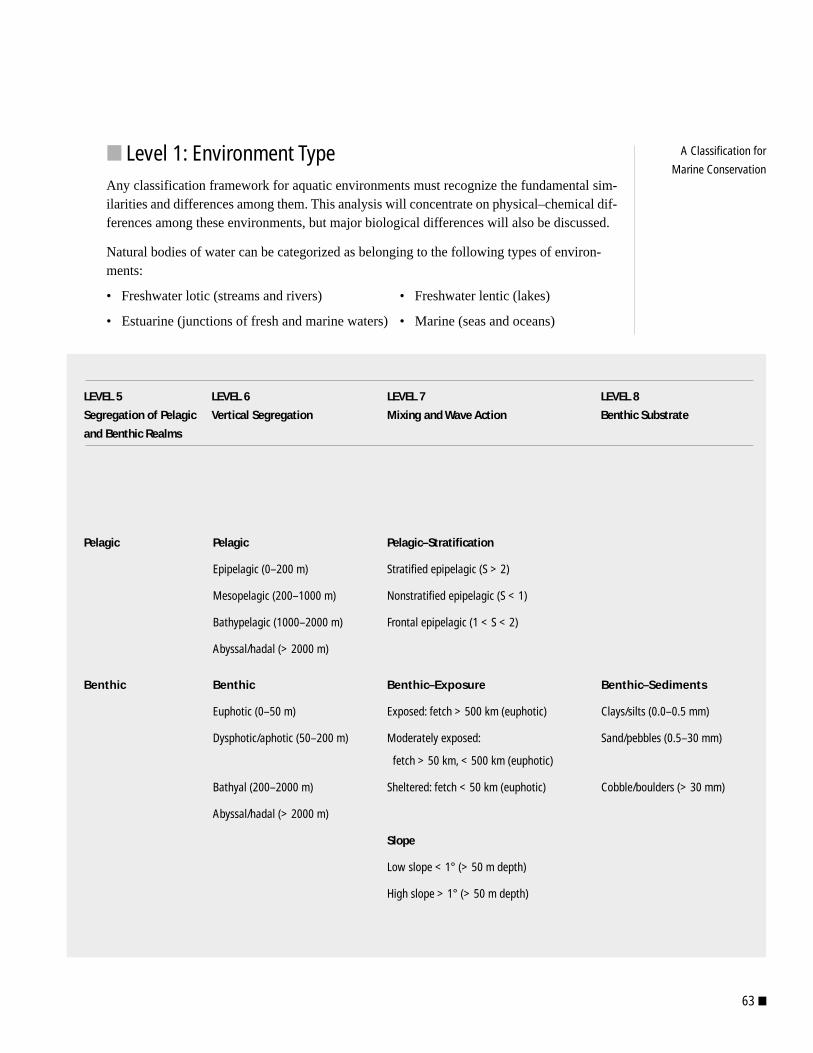
63 ■

A Classification for

Marine Conservation ■ Level 1: Environment TypeAny classification framework for aquatic environments must recognize the fundamental sim-ilarities and differences among them. This analysis will concentrate on physical–chemical dif-ferences among these environments, but major biological differences will also be discussed.

Natural bodies of water can be categorized as belonging to the following types of environ-ments:

• Freshwater lotic (streams and rivers) • Freshwater lentic (lakes)

• Estuarine (junctions of fresh and marine waters) • Marine (seas and oceans)

Pelagic Pelagic Pelagic–Stratification

Epipelagic (0–200 m) Stratified epipelagic (S > 2)

Mesopelagic (200–1000 m) Nonstratified epipelagic (S < 1)

Bathypelagic (1000–2000 m) Frontal epipelagic (1 < S < 2)

Abyssal/hadal (> 2000 m)

Benthic Benthic Benthic–Exposure Benthic–Sediments

Euphotic (0–50 m) Exposed: fetch > 500 km (euphotic) Clays/silts (0.0–0.5 mm)

Dysphotic/aphotic (50–200 m) Moderately exposed: Sand/pebbles (0.5–30 mm)

fetch > 50 km, < 500 km (euphotic)

Bathyal (200–2000 m) Sheltered: fetch < 50 km (euphotic) Cobble/boulders (> 30 mm)

Abyssal/hadal (> 2000 m)

Slope

Low slope < 1° (> 50 m depth)

High slope > 1° (> 50 m depth)

LEVEL 5 LEVEL 6 LEVEL 7 LEVEL 8

Segregation of Pelagic Vertical Segregation Mixing and Wave Action Benthic Substrate

and Benthic Realms

■ 64

Planning for

Representative Marine

Protected Areas:

A Framework for

Canada’s Oceans

While the above aquatic environments have many features in common, each has its ownunique set of properties and its own suite of relationships between geophysical characteris-tics and biological communities. Although some relationships may traverse the boundariesof environment type, it would be a mistake to extrapolate relationships uncritically fromone environment type to another. Thus, while a similar framework for the hierarchical clas-sification of each of these groups of aquatic environments could be developed on the basisof the same fundamental principles, each would require a different array of factors in itsown hierarchical classification. This has not been done here, but a classification frameworkfor the Great Lakes is currently in development.

This report and framework outlines a classification system only for the marine environ-ment. There is no perfect definition of what constitutes the marine environment. Since itdominates our planet, a more relevant question might be, What does not constitute part ofthe marine environment? For the purposes of this framework, the marine environment isconsidered to include oceans, seas, bays and the outer reaches of estuaries where the ambi-ent salinity exceeds about 30 parts per thousand. Thus we are considering all those marinewaters of full-strength salinity or where dilution by fresh water amounts to only about 10per cent.

■ Level 2: Geographic RangeEach of the three oceans surrounding Canada contains its own distinct complement anddiversity of species. These species, however, are arrayed within the same recognizable setsor assemblages of species (i.e., communities). Although the species themselves differ, wecan still recognize the same community types. We can also recognize the same ecosystem-level dynamics in all three oceans. The Pacific Ocean, with its longer evolutionary history,has a richer species diversity and more distinct species assemblages than the Arctic andAtlantic Oceans. The Atlantic coast of Canada is strongly affected by the westward-intensi-fied currents of the subpolar and subtropical gyres—the Gulf Stream and the LabradorCurrent respectively. In contrast, the Pacific coast of Canada lies under the eastern watersof corresponding gyres, with weaker currents producing a temperate area that is transition-al in character between arctic and subtropical waters.

The exchange of water between the Arctic and Atlantic Oceans is substantial, with deepAtlantic Ocean waters reaching to the mouth of Hudson Bay and surface Arctic Oceanwaters affecting the Scotian Shelf. Thus the division between these oceans is as much a ver-tical as a horizontal phenomenon. In contrast, in the Pacific Ocean, the narrow and shallowBering Strait substantially reduces the exchange between the Arctic and Pacific Oceans.

The division between the Arctic and Atlantic Oceans used in this framework is based onsea-ice frequency and the previously defined extents of the Arctic and Atlantic basins(Dunbar 1968; Brown et al. 1975).

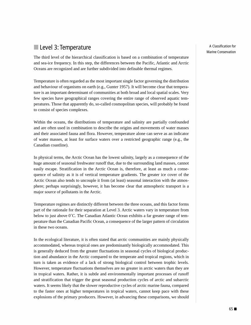
65 ■

A Classification for

Marine Conservation ■ Level 3: TemperatureThe third level of the hierarchical classification is based on a combination of temperatureand sea-ice frequency. In this step, the differences between the Pacific, Atlantic and ArcticOceans are recognized and are further subdivided into definable thermal regimes.

Temperature is often regarded as the most important single factor governing the distributionand behaviour of organisms on earth (e.g., Gunter 1957). It will become clear that tempera-ture is an important determinant of communities at both broad and local spatial scales. Veryfew species have geographical ranges covering the entire range of observed aquatic tem-peratures. Those that apparently do, so-called cosmopolitan species, will probably be foundto consist of species complexes.

Within the oceans, the distributions of temperature and salinity are partially confoundedand are often used in combination to describe the origins and movements of water massesand their associated fauna and flora. However, temperature alone can serve as an indicatorof water masses, at least for surface waters over a restricted geographic range (e.g., theCanadian coastline).

In physical terms, the Arctic Ocean has the lowest salinity, largely as a consequence of thehuge amount of seasonal freshwater runoff that, due to the surrounding land masses, cannoteasily escape. Stratification in the Arctic Ocean is, therefore, at least as much a conse-quence of salinity as it is of vertical temperature gradients. The greater ice cover of theArctic Ocean also tends to uncouple it from (at least) seasonal interaction with the atmos-phere; perhaps surprisingly, however, it has become clear that atmospheric transport is amajor source of pollutants in the Arctic.

Temperature regimes are distinctly different between the three oceans, and this factor formspart of the rationale for their separation at Level 3. Arctic waters vary in temperature frombelow to just above 0˚C. The Canadian Atlantic Ocean exhibits a far greater range of tem-perature than the Canadian Pacific Ocean, a consequence of the larger pattern of circulationin these two oceans.

In the ecological literature, it is often stated that arctic communities are mainly physicallyaccommodated, whereas tropical ones are predominantly biologically accommodated. Thisis generally deduced from the greater fluctuations in seasonal cycles of biological produc-tion and abundance in the Arctic compared to the temperate and tropical regions, which inturn is taken as evidence of a lack of strong biological control between trophic levels.However, temperature fluctuations themselves are no greater in arctic waters than they arein tropical waters. Rather, it is subtle and environmentally important processes of runoffand stratification that trigger the great seasonal production cycles of arctic and subarcticwaters. It seems likely that the slower reproductive cycles of arctic marine fauna, comparedto the faster ones at higher temperatures in tropical waters, cannot keep pace with theseexplosions of the primary producers. However, in advancing these comparisons, we should

■ 66

Planning for

Representative Marine

Protected Areas:

A Framework for

Canada’s Oceans

be aware that our perceptions are coloured by two things: first, there is considerable confu-sion between the Arctic proper and the subarctic region, and second, we have far greaterunderstanding of terrestrial than of marine arctic biological processes. Most of our know-ledge, in fact, derives from the terrestrial subarctic regions.

Subarctic, boreal and temperate waters typically support the greatest commercial fisheries.Production is lower in arctic waters because of lower temperatures, lower plant productivi-ty and the short growing season. Production is typically lower in tropical waters because ofpermanent vertical stratification that prevents significant return of nutrients to surfacewaters.

ARCTIC WATERS

Separation of arctic and subarctic waters largely follows Dunbar (1968). In the Antarctic,polar and subpolar waters are readily distinguished; indeed, they are physically separatedby a temperature discontinuity at the Antarctic convergence. Separation in the Arctic is notso dramatic, and characteristics of surface waters can be variable. Indeed, the subarcticzone has no true counterpart in the southern hemisphere. Arctic waters typically remain ator below 0˚C throughout the year. They generally remain vertically stratified throughoutthe year, predominantly as a result of salinity stratification. A large part of the Arctic Oceanremains ice covered throughout the year, and floating ice is typical throughout the year.Marine arctic waters have a lower productivity and lower species diversity than marinesubarctic waters.

SUBARCTIC WATERS

Although ice generally forms at the surface during the winter, the water mass of the marinesubarctic zone generally remains above 0˚C throughout the year. This zone is generally freeof ice during the summer, except for adventitious floes and icebergs. The marine subarcticzone is more productive and displays greater species diversity than arctic waters. Subarcticwaters may be highly productive during the summer months or where areas remain ice free,depending on the local regime of mixing and upwelling. Such mixing may be tidally ortopographically induced, or prevented by the reduced salinity of surface waters. The sea-icecommunity itself (the epontic community) may be a significant source of fundamentalnutrition for many migratory species of fish and marine mammals.

BOREAL WATERS

The boreal zone exhibits moderate ice frequency and generally low summer maximumtemperatures. Ice is expected to occur for at least one month and last up to six months, andthe average annual temperature is above 0˚C. This zone is unique due to colder arcticwaters flowing from the north above warmer temperate waters flowing from the south.Boreal waters may be highly productive during the summer months. Fish and marine mam-mal species (or their subpopulations) may be widely distributed and range widely.

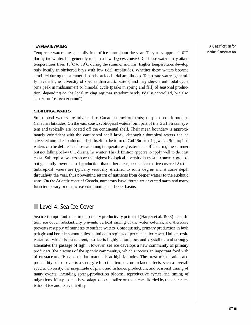
67 ■

A Classification for

Marine Conservation

TEMPERATE WATERS

Temperate waters are generally free of ice throughout the year. They may approach 0˚Cduring the winter, but generally remain a few degrees above 0˚C. These waters may attaintemperatures from 15˚C to 18˚C during the summer months. Higher temperatures developonly locally in sheltered bays with low tidal amplitudes. Whether these waters becomestratified during the summer depends on local tidal amplitudes. Temperate waters general-ly have a higher diversity of species than arctic waters, and may show a unimodal cycle(one peak in midsummer) or bimodal cycle (peaks in spring and fall) of seasonal produc-tion, depending on the local mixing regimes (predominantly tidally controlled, but alsosubject to freshwater runoff).

SUBTROPICAL WATERS

Subtropical waters are advected to Canadian environments; they are not formed atCanadian latitudes. On the east coast, subtropical waters form part of the Gulf Stream sys-tem and typically are located off the continental shelf. Their mean boundary is approxi-mately coincident with the continental shelf break, although subtropical waters can beadvected onto the continental shelf itself in the form of Gulf Stream ring water. Subtropicalwaters can be defined as those attaining temperatures greater than 18˚C during the summerbut not falling below 6˚C during the winter. This definition appears to apply well to the eastcoast. Subtropical waters show the highest biological diversity in most taxonomic groups,but generally lower annual production than other areas, except for the ice-covered Arctic.Subtropical waters are typically vertically stratified to some degree and at some depththroughout the year, thus preventing return of nutrients from deeper waters to the euphoticzone. On the Atlantic coast of Canada, numerous larval forms are advected north and manyform temporary or distinctive communities in deeper basins.

■ Level 4: Sea-Ice CoverSea ice is important in defining primary productivity potential (Harper et al. 1993). In addi-tion, ice cover substantially prevents vertical mixing of the water column, and thereforeprevents resupply of nutrients to surface waters. Consequently, primary production in bothpelagic and benthic communities is limited in regions of permanent ice cover. Unlike fresh-water ice, which is transparent, sea ice is highly amorphous and crystalline and stronglyattenuates the passage of light. However, sea ice develops a new community of primaryproducers (the diatoms of the epontic community), which supports an important food webof crustaceans, fish and marine mammals at high latitudes. The presence, duration andprobability of ice cover is a surrogate for other temperature-related effects, such as overallspecies diversity, the magnitude of plant and fisheries production, and seasonal timing ofmany events, including spring-production blooms, reproductive cycles and timing ofmigrations. Many species have adapted to capitalize on the niche afforded by the character-istics of ice and its availability.

■ 68

Planning for

Representative Marine

Protected Areas:

A Framework for

Canada’s Oceans

PERMANENT PACK ICE

Permanent pack ice is defined as the area where no regular breakup of ice occurs and whereless than 25 per cent of the total ice mass is new ice. Very low levels of production areexpected to occur in areas of permanent sea ice.

SEASONAL ICE

Seasonal ice is expected to occur annually with a probability of 9 out of 10 years at the out-ermost extent of the zone. The ice is expected to last five to six months per year at its limit.This zone contains a combination of pack ice and first-year drift ice. Slightly higher pro-ductivity is expected in this zone relative to areas of permanent pack ice.

VARIABLE ICE

Separation of variable ice from seasonal ice is important, since this zone of variable ice rep-resents a transitional area with a high degree of variation in average annual temperature andpotential ice cover. In this zone, the probability of ice forming in a given year is between 25per cent and 90 per cent (i.e., on average, annual sea-ice formation occurs from 2.5 yearsout of 10 to 9 years out of 10). Moderate productivity is expected in areas of variable icecover.

NO ICE

Areas where no sea ice occurs are contained within temperate and subtropical waters. Theprobability of sea ice forming in a given year is less than 25 per cent in these areas (i.e., onaverage, sea ice forms in fewer than 2.5 years out of 10). The absence of ice allows forgreater productivity relative to areas where ice is present.

POLYNYAS

Polynyas are unique phenomena defined as enduring ice-free areas surrounded by ice. Theyare zones of much higher productivity relative to adjacent habitat.

■ Level 5: Segregation of Pelagic and Benthic RealmsMarine systems are significantly different from terrestrial systems in having two separaterealms with functionally different communities:

• Pelagic communities encompass all those organisms that inhabit the water column itself.

• Benthic communities encompass all those organisms that inhabit the substrates of aquatic basins.

Note that at the scale of mapping used in this study, species that are demersal will be con-sidered as effectively benthic.

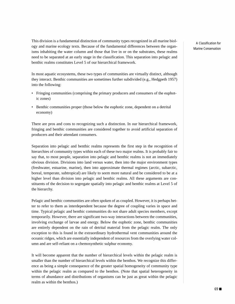
69 ■

A Classification for

Marine Conservation

This division is a fundamental distinction of community types recognized in all marine biol-ogy and marine ecology texts. Because of the fundamental differences between the organ-isms inhabiting the water column and those that live in or on the substrates, these realmsneed to be separated at an early stage in the classification. This separation into pelagic andbenthic realms constitutes Level 5 of our hierarchical framework.

In most aquatic ecosystems, these two types of communities are virtually distinct, althoughthey interact. Benthic communities are sometimes further subdivided (e.g., Hedgpeth 1957)into the following:

• Fringing communities (comprising the primary producers and consumers of the euphot-ic zones)

• Benthic communities proper (those below the euphotic zone, dependent on a detritaleconomy)

There are pros and cons to recognizing such a distinction. In our hierarchical framework,fringing and benthic communities are considered together to avoid artificial separation ofproducers and their attendant consumers.

Separation into pelagic and benthic realms represents the first step in the recognition ofhierarchies of community types within each of these two major realms. It is probably fair tosay that, to most people, separation into pelagic and benthic realms is not an immediatelyobvious division. Divisions into land versus water, then into the major environment types(freshwater, estuarine, marine), then into approximate thermal regimes (arctic, subarctic,boreal, temperate, subtropical) are likely to seem more natural and be considered to be at ahigher level than division into pelagic and benthic realms. All these arguments are con-stituents of the decision to segregate spatially into pelagic and benthic realms at Level 5 ofthe hierarchy.

Pelagic and benthic communities are often spoken of as coupled. However, it is perhaps bet-ter to refer to them as interdependent because the degree of coupling varies in space andtime. Typical pelagic and benthic communities do not share adult species members, excepttemporarily. However, there are significant two-way interactions between the communities,involving exchange of larvae and energy. Below the euphotic zone, benthic communitiesare entirely dependent on the rain of detrital material from the pelagic realm. The onlyexception to this is found in the extraordinary hydrothermal vent communities around theoceanic ridges, which are essentially independent of resources from the overlying water col-umn and are self-reliant on a chemosynthetic sulphur economy.

It will become apparent that the number of hierarchical levels within the pelagic realm issmaller than the number of hierarchical levels within the benthos. We recognize this differ-ence as being a simple consequence of the greater spatial homogeneity of community typewithin the pelagic realm as compared to the benthos. (Note that spatial heterogeneity interms of abundance and distributions of organisms can be just as great within the pelagicrealm as within the benthos.)

■ 70

Planning for

Representative Marine

Protected Areas:

A Framework for

Canada’s Oceans

■ Level 6: Vertical SegregationWithin the water column, depth, pressure, light penetration and turbidity are all interrelat-ed. From the shoreline to the continental shelf to offshore areas beyond the continentalslope, water-column depth increases, light penetrates farther (because of greater water clar-ity and lower turbidity) and pressure increases. Along this continuum, we pass from coastalto neritic to progressively more oceanic communities.

PELAGIC REALM

Community structure changes greatly with depth as we pass below the euphotic zone andencounter the larger pelagic species whose populations may be concentrated into discretelayers but nevertheless become progressively less common with depth.

Water-column depth itself acts as a suitable discriminant of community type and alsoaccounts for the correlated factors of light penetration and pressure. Seasonal thermal strat-ification is relevant only to the upper 200 metres of the water column. Below this, the watercolumn almost always exhibits some form of stratification (due to changes in temperatureand/or salinity), but seasonal variations become negligible due to the great homogenizingeffects of ocean circulation and the high heat capacity of water.

The natural classification of the pelagic environment that emerges from these considera-tions is as follows:

1. Segregate the water column by depth intervals at Level 6.

2. Segregate the pelagic zone into stratified, nonstratified and frontal regions at Level 7.

The depth intervals chosen are those generally recognized in the biological oceanographicliterature as separating communities that show clear differences in species composition.

Two further points should be made:

1. Vertical migration by the animals of the pelagic realm obviously integrates trophody-namic processes within these communities in the vertical plane. Nevertheless, verticalstructure in these communities is clearly defined and should be recognized as a corre-late of increasing water-column depth.

2. We would hardly expect that an MPA would encompass only, for example, the 1000-metre to 2000-metre depth interval of the water column. However, separate recognitionof these different communities as occupying different strata, their natural correlationwith water depth and the parallel classification of benthic communities should makesubsequent selection of MPAs a more orderly process.

71 ■

A Classification for

Marine Conservation

BENTHIC REALM

At Level 6 of the benthic hierarchy, the factor that discriminates most significantly betweencommunity types is depth, which is a correlate of light and pressure. Depth is chosen as thesimplest index of these interacting effects. Thus the intertidal community is typically rich inmacrophytic and microphytic plants and shelters a wide diversity of organisms adapted torecurrent immersion and exposure. Below this, but still within the euphotic zone, lie well-recognized community types where plant growth (again either macrophytic or microphytic)can thrive. Below the euphotic zone, resources for animals are dependent on detrital inputsfrom the euphotic zone, and the coarsest substrates are generally lost in favour of finer sed-imentary ones. Figure 2 illustrates the depth intervals of the pelagic and benthic zones.

■ Level 7: Mixing and Wave ActionLevel 7 identifies the effects of water motion on both the pelagic and benthic realms. Tidalcurrents and wave action can cause stratified waters to mix, thus affecting nutrient supplyand turbidity. Wave action also affects the substrate type, especially in exposed or high-slope areas. These effects of water motion play a significant role in the distribution ofmarine communities.

PELAGIC STRATIFICATION

At scales from metres to hundreds of kilometres, the pelagic realm may appear to be large-ly homogeneous until more closely examined. A major feature of the pelagic realm is itsspatial heterogeneity, generally referred to as patchiness. However, specialized samplingapparatus is needed to reveal these quantitative heterogeneities. Pelagic species demon-strate a great diversity of body size, form and taxonomic type (i.e., a high diversity of phylainhabit the pelagic realm), but species diversity itself tends to be lower than in the benthos,perhaps as a function of qualitative environmental homogeneity. The pelagic realm itselfcan be vertically subdivided, as discussed above.

Figure 2. PELAGIC AND BENTHIC ZONES OF THE OCEAN

3

4

5

6

2Water Surface1

1. Nearshore euphotic (0–50 m)

2. Pelagic euphotic/epipelagic (0–50 m)

3. Dysphotic/epipelagic (50–200 m)

4. Aphotic/mesopelagic (200–1000 m)

5. Aphotic/bathypelagic (1000–2000 m)

6. Aphotic/abyssal (> 2000 m)

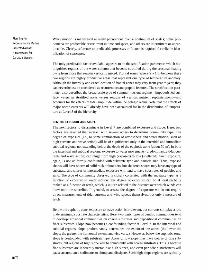
■ 72

Planning for

Representative Marine

Protected Areas:

A Framework for

Canada’s Oceans

Water motion is manifested in many phenomena over a continuum of scales; some phe-nomena are predictable or recurrent in time and space, and others are intermittent or unpre-dictable. Clearly, reference to predictable processes or factors is required for reliable iden-tification of seascapes.

The only predictable factor available appears to be the stratification parameter, which dis-tinguishes regions of the water column that become stratified during the seasonal heatingcycle from those that remain vertically mixed. Frontal zones (where S ~ 1.5) between thesetwo regions are highly productive areas that represent one type of temperature anomaly.Although the intensity and exact location of frontal zones may vary from year to year, theycan nevertheless be considered as recurrent oceanographic features. The stratification para-meter also describes the broad-scale type of summer nutrient regime—impoverished sur-face waters in stratified areas versus regions of vertical nutrient replenishment—andaccounts for the effects of tidal amplitude within the pelagic realm. Note that the effects ofmajor ocean currents will already have been accounted for in the distribution of tempera-ture at Level 3 of the hierarchy.

BENTHIC EXPOSURE AND SLOPE

The next factors to discriminate in Level 7 are combined exposure and slope. Here, twofactors are selected that interact with several others to determine community type. Thedegree of exposure (i.e., to some combination of atmosphere and water motion, such ashigh currents and wave action) will be of significance only in the intertidal and immediatesubtidal regions, not extending below the depth of the euphotic zone (about 50 m). In boththe intertidal and subtidal regions, exposure to water movements (predominantly tidal cur-rents and wave action) can range from high (exposed) to low (sheltered). Such exposure,again, is not uniformly confounded with substrate type and particle size. Thus, exposedshores will have shores of solid rock or boulders, but sheltered shores may have any type ofsubstrate, and shores of intermediate exposure will tend to have substrates of pebbles andsand. The type of community observed is closely correlated with the substrate type, as afunction of exposure to water motion. The degree of exposure can be at least partiallyranked as a function of fetch, which is in turn related to the distance over which winds canblow onto the shoreline. In general, to assess the degree of exposure we do not requiredirect measurements of tidal currents and wind speeds themselves, but only a measure offetch.

Below the euphotic zone, exposure to wave action is irrelevant, but currents still play a rolein determining substrate characteristics. Here, two basic types of benthic communities tendto develop: erosional communities on coarse substrates and depositional communities onfiner substrates. Slope now becomes a confounding factor at Level 7. In the intertidal andsubtidal regions, slope predominantly determines the extent of the zones (the lower theslope, the greater the horizontal extent, and vice versa). However, below the euphotic zone,slope is confounded with substrate type. Areas of low slope may have coarse or fine sub-strates, but regions of high slope will be found only with coarse substrates. This is becausefine substrates are inherently unstable at high slopes, and even periodic disturbances willcause accumulated sediments to slump and dissipate. Such high-slope regions are typically

73 ■

A Classification for

Marine Conservation

associated with the edge of the continental shelf, with sea mounts that rise above the sur-rounding bottom and with canyons that descend below it. Typically, such areas also experi-ence the effects of local currents more than the surrounding flat plains, and may developbenthic communities that differ significantly from those of regions of finer substrates atsimilar depths. Thus slope may sometimes act as a partial surrogate for substrate particlesize.

■ Level 8: Benthic SubstrateHabitat types in Level 8 are discriminated according to substrate type. This factor itself is,of course, partially confounded with depth. In shallow waters, substrates span the size spec-trum from solid rock to fine sediments, depending on the energy of local water motion. Indeeper waters, the energy associated with water motion is greatly reduced and sedimentarysubstrates predominate. With increasing depth, the strong tendency is for sediments tobecome progressively finer in particle size and to have lower organic contents until, in thedeepest parts of the ocean, sediments have become almost uniformly similar in mud and siltcomposition.

The increasing uniformity of substrate type with increasing depth means that in deep off-shore areas the benthos tends to converge to only a few community types, and many speciesmay be cosmopolitan. Typical species include a variety of deposit feeders, especially tube-building polychaete worms and bivalve molluscs and small epibenthic or burrowing crus-taceans. Coarse-textured substrates are typically found in areas of stronger currents wheresuspension feeders predominate. Here, larger surface-dwelling bivalves and echinodermsmay be most evident, along with a diversity of other taxa, such as sponges, sea stars,decapods and other motile forms. Medium-textured substrates often indicate conditions andcommunity types intermediate between deposit-feeding and suspension-feeding communi-ties, and may be heavily dominated by small clams, brittle stars or ascideans. Where suchsubstrates are kept in motion by the action of currents, the abrasive forces may greatlyreduce the local biological diversity of larger plant and invertebrate species.

3c

■ 74

Planning for

Representative Marine

Protected Areas:

A Framework for

Canada’s Oceans

Data Requirements forDetermining Seascapes

■ IntroductionOne of the strengths of a classification based on physiographic and oceanographic featuresis that data relating to these features tend to be more consistent and readily available at anational scale than do biological data. Table 4 outlines, to the best of our knowledge, wherethe data necessary for the classification of seascapes can be found. However, there may beinstances, especially in the Arctic, where data are simply not available at the appropriatescale. In such cases, decisions will need to be based on the best available information, andan adaptive management approach should be adopted that allows better information to beincorporated as it becomes available.

Table 4. DATA REQUIREMENTS FOR THE CLASSIFICATION OF MARINE SEASCAPES IN CANADA

Factor Location Classes/Description Source of Map/GIS Datain Framework Used in Framework

Environment type Level 1 Marine—all oceanic waters Marine waters can be mapped usingsubject to tidal influences, either topographic maps or hydrographic including the St. Lawrence charts.River

Geographic range Level 2 Arctic Ocean The distinction between the Atlantic Atlantic Ocean and Pacific Oceans is based on previouslyPacific Ocean defined extents of the Arctic and

Atlantic basins (Dunbar 1968; Brown et al. 1975).

Temperature Level 3 Arctic Arctic (avg. temp. < 0°C, ice 9–12 monthsSubarctic Subarctic (avg. temp. > 0°C, ice 6–9 months)Boreal Boreal (avg. temp. > 0°C, ice 1–6 months)Temperate Temperate (avg. temp. > 0°C, < 18°C,

ice < 1 month)Subtropical Subtropical (avg. temp. > 6°C winter,

> 18°C summer)

Sea-ice cover Level 4 Permanent ice cover Use National Atlas of Canada sea-ice map.Seasonal ice coverVariable ice coverAbsent (includes polynyas)

Segregation of Level 5 Pelagic This is a theoretical and management principle pelagic and Benthic and does not require spatial data to benthic realms segregate realms.

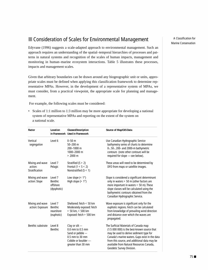
75 ■

A Classification for

Marine Conservation

Factor Location Classes/Description Source of Map/GIS Datain Framework Used in Framework

Vertical Level 6 0–50 m Use Canadian Hydrographic Service segregation 50–200 m bathymetry series of charts to determine

200–1000 m 0-, 50-, 200- and 2000-m bathymetric 1000–2000 m contours (note other contours will be > 2000 m required for slope —see below).

Mixing and wave Level 7 Stratified (S > 2) These areas will need to be determined by action: Pelagic Frontal (1 < S < 2) DFO from maps or satellite images.

Stratification Nonstratified (S < 1)

Mixing and wave Level 7 Low slope (< 1°) Slope is considered a significant determinantaction: Slope Benthic High slope (> 1°) only in waters > 50 m (other factors are

offshore more important in waters < 50 m). These (dysphotic) slope classes will be calculated using the

bathymetric contours obtained from the Canadian Hydrographic Service.

Mixing and wave Level 7 Sheltered: fetch < 50 km Wave exposure is significant only for the action: Exposure Benthic Moderately exposed: fetch euphotic regions. Fetch can be calculated

nearshore > 50 km, < 500 km from knowledge of prevailing wind direction (euphotic) Exposed: fetch > 500 km and distance over which the waves are

propagated.

Benthic substrate Level 8 Clay or silt — The Surficial Materials of Canada map Benthic 0.0 mm to 0.5 mm (1:5 000 000) is the best-known source that

Sand or pebble — may be used to derive sediment type for 0.5 mm to 30 mm Canada’s marine waters. Gaps exist in the data Cobble or boulder — from this source, and additional data may be greater than 30 mm available from Natural Resources Canada,

Geodetic Survey Division.

■ Consideration of Scales for Environmental ManagementEdyvane (1996) suggests a scale-adapted approach to environmental management. Such anapproach requires an understanding of the spatial–temporal hierarchies of processes and pat-terns in natural systems and recognition of the scales of human impacts, management andmonitoring in human–marine ecosystem interactions. Table 5 illustrates these processes,impacts and management scales.

Given that arbitrary boundaries can be drawn around any biogeographic unit or units, appro-priate scales must be defined when applying this classification framework to determine rep-resentative MPAs. However, in the development of a representative system of MPAs, wemust consider, from a practical viewpoint, the appropriate scale for planning and manage-ment.

For example, the following scales must be considered:

• Scales of 1:1 million to 1:3 million may be more appropriate for developing a nationalsystem of representative MPAs and reporting on the extent of the system on a national scale.

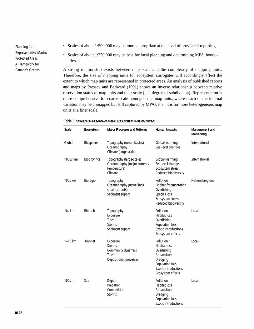
■ 76

Planning for

Representative Marine

Protected Areas:

A Framework for

Canada’s Oceans

• Scales of about 1:500 000 may be more appropriate at the level of provincial reporting.

• Scales of about 1:250 000 may be best for local planning and determining MPA bound-aries.

A strong relationship exists between map scale and the complexity of mapping units.Therefore, the size of mapping units for ecosystem surrogates will accordingly affect theextent to which map units are represented in protected areas. An analysis of published reportsand maps by Pressey and Bedward (1991) shows an inverse relationship between relativereservation status of map units and their scale (i.e., degree of subdivision). Representation ismore comprehensive for coarse-scale homogeneous map units, where much of the internalvariation may be unmapped but still captured by MPAs, than it is for more heterogeneous mapunits at a finer scale.

Table 5. SCALES OF HUMAN–MARINE ECOSYSTEM INTERACTIONS

Scale Ecosystem Major Processes and Patterns Human Impacts Management and Monitoring

Global Biosphere Topography (ocean basins) Global warming InternationalOceanography Sea-level changes Climate (large-scale)

1000s km Bioprovince Topography (large-scale) Global warming International Oceanography (major currents, Sea-level changestemperature) Ecosystem stress Climate Reduced biodiversity

100s km Bioregion Topography Pollution National/regional Oceanography (upwellings, Habitat fragmentationsmall currents) OverfishingSediment supply Species loss

Ecosystem stressReduced biodiversity

10s km Bio-unit Topography Pollution LocalExposure Habitat loss Tides OverfishingStorms Population lossSediment supply Exotic introductions

Ecosystem effects

1–10 km Habitat Exposure Pollution LocalStorms Habitat lossCommunity dynamics OverfishingTides AquacultureDepositional processes Dredging

Population lossExotic introductionsEcosystem effects

100s m Site Depth Pollution Local Predation Habitat lossCompetition AquacultureStorms Dredging

Population loss` Exotic introductions

77 ■

A Classification for

Marine Conservation 3dAssumptions, Limitations and Caveats

■ IntroductionFrameworks and classifications provide a valuable and meaningful basis for aggregatinginformation, depicting patterns, mapping marine representative areas and setting priorities.While the approach used here is flexible, repeatable and hierarchical, it is important, howev-er, to understand what assumptions, limitations and caveats pertain to the overall frameworkand the resulting classifications.

■ Assumptions and LimitationsAssumption 1: The ecosystem- and species-level approaches frequently applied to marine

conservation are inherently unworkable at broad (i.e., national) scales.

Limitation: These approaches to conservation have been adopted elsewhere. Two majorchallenges with such approaches for MPA planning are that natural bound-aries between marine ecosystems generally cannot be consistently defined,and that there is no clear way to combine mapping data for individual speciesdistributions. These challenges make it difficult to set goals or targets forcompleting an MPA system.

Assumption 2: The framework presented in this report is an ecological hierarchy of habi-tats; it is not a spatial hierarchy of habitats.

Limitation: Correspondence between habitat type and spatial scale is, therefore, unavoid-ably lost. The natural patterns of spatial organization of biological communi-ties must be recognized in proceeding from seascapes to the selection ofMPAs.

Assumption 3: By identifying habitat types, we can produce, as far as practicable, a sys-tematic basis for helping to conserve marine biodiversity. If we can identi-fy the appropriate range of habitat conditions, then these should contain amajority of the species we wish to preserve.

Limitation: By identifying and conserving habitat types, a systematic framework for con-servation can be developed that represents, either directly or indirectly, bio-logical diversity at the community level. However, the seascape framework

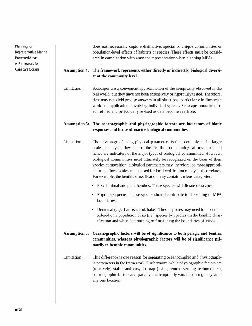
■ 78

Planning for

Representative Marine

Protected Areas:

A Framework for

Canada’s Oceans

does not necessarily capture distinctive, special or unique communities orpopulation-level effects of habitats or species. These effects must be consid-ered in combination with seascape representation when planning MPAs.

Assumption 4: The framework represents, either directly or indirectly, biological diversi-ty at the community level.

Limitation: Seascapes are a convenient approximation of the complexity observed in thereal world, but they have not been extensively or rigorously tested. Therefore,they may not yield precise answers in all situations, particularly in fine-scalework and applications involving individual species. Seascapes must be test-ed, refined and periodically revised as data become available.

Assumption 5: The oceanographic and physiographic factors are indicators of bioticresponses and hence of marine biological communities.

Limitation: The advantage of using physical parameters is that, certainly at the largerscale of analysis, they control the distribution of biological organisms andhence are indicators of the major types of biological communities. However,biological communities must ultimately be recognized on the basis of theirspecies composition; biological parameters may, therefore, be more appropri-ate at the finest scales and be used for local verification of physical correlates.For example, the benthic classification may contain various categories:

• Fixed animal and plant benthos: These species will dictate seascapes.

• Migratory species: These species should contribute to the setting of MPAboundaries.

• Demersal (e.g., flat fish, cod, hake): These species may need to be con-sidered on a population basis (i.e., species by species) in the benthic class-ification and when determining or fine-tuning the boundaries of MPAs.

Assumption 6: Oceanographic factors will be of significance to both pelagic and benthiccommunities, whereas physiographic factors will be of significance pri-marily to benthic communities.

Limitation: This difference is one reason for separating oceanographic and physiograph-ic parameters in the framework. Furthermore, while physiographic factors are(relatively) stable and easy to map (using remote sensing technologies),oceanographic factors are spatially and temporally variable during the year atany one location.

79 ■

A Classification for

Marine Conservation

Assumption 7: Different relationships will exist between the identified seascapes and thecandidate MPAs that may be selected in any area.

Limitation: Because this framework is an ecological hierarchy and not a spatial one,seascapes will vary considerably in size from one region to another andbetween realms, depending on the natural heterogeneity of a region and theorganization of its representative community types. Thus it should be expect-ed that in some areas a representative MPA will be contained wholly within agiven seascape, whereas in other areas an MPA may contain several smallerseascapes. A prime example of the first case would be in pelagic areas or thedeep-sea benthos, and a good example of the second case would be a sectionof coastline, that comprises rocky shores, sandy beaches and sheltered muddybays. Thus, moving from deep to shallow waters, we would probably expectthe following transition:

• Deep water: Several MPAs each contained within a seascape

• Shallow water: An MPA containing several seascapes

Assumption 8: Even when the seascape analysis is complete, a further process is requiredto proceed from seascapes to MPAs; distinctive areas, special needs andpracticalities must be considered in this process.

Limitation: While a scientific rationale exists for the delineation of seascapes and candi-date MPAs, the integration of further ecological, socioeconomic, legal andpolitical aspects, and practicalities makes the final selection and design ofMPAs subjective and more of an art than a science. Furthermore, processes atboth the population level (e.g., migrant species) and the ecosystem level mustbe considered to determine what may have been missed at the seascape level.

Assumption 9: Certain oceanographic and physiographic data are available for mapping.

Limitation: The data used to derive seascapes are the best available to WWF Canada;where data are not available, surrogates have been used wherever possible.For some areas, all types of data (including surrogates) are limited or notavailable; in these instances, other approaches must be applied (e.g., model-ling).

Assumption 10: Data must be available, either directly or via suitable surrogates at compa-rable scales, for all areas to be evaluated to ensure consistency of interpre-tation and comparison.

■ 80

Planning for

Representative Marine

Protected Areas:

A Framework for

Canada’s Oceans

Limitation: Considerable effort has been invested in the interpretation of data and infor-mation used to determine seascapes. Some instances occur, however, in whichthe scale, type and number of attributes used, the temporal differencesbetween data sets, and the different analytical methods used will affect theappropriateness of the data for comparison between areas (e.g., betweenoceans).

Assumption 11: The relationships between communities and their physical environmentare the same in all three oceans, and equivalent community types consist ofthe same sets of “ecological species,” that is, species guilds or trophos-pecies.

Limitation: Until more detailed information is known, this assumption can be made. Notethat if we can verify that similar community types do, in fact, exist, we couldanswer questions such as, Is the greater species diversity of the Pacific Oceanreflected in a greater diversity of community types or simply a greater speciesdiversity within them?

Assumption 12: The delineation of seascapes as described embodies a single frameworkthat integrates both pelagic and benthic realms. It accounts for differenti-ation on the basis of pelagic and benthic communities and for differentia-tion of light regimes based on euphotic and aphotic zones.

Limitation: The benthic and pelagic regions have been identified on the basis of availableknowledge, using a variety of approaches to delineate the boundaries. The factthat the benthic and pelagic classifications are separate requires some integra-tion for the final depiction of seascapes. While this integration is assisted byoverlaying the two classifications, some subjective interpretation is requiredto determine the final seascape boundaries. These integrated boundaries mustcontinually be tested and validated using a range of regional and continentaldata sets and analytical tools.

Assumption 13: The degree of actual affinity between physical and biological attributes hasnot yet been rigorously tested for all communities.

Limitation: This affinity should be tested for all communities and the results used to refinethe framework.

Assumption 14: The habitat types identified are discrete types as opposed to continuousecological gradients. We have not considered whether gradients betweenhabitat types are just as important as or more important than habitattypes or whether such gradients should formally enter the analysis.

Limitation: The habitat types identified are not simply “fuzzy” boundaries around a dis-junction. On the contrary, some of the ecotones may be as extensive as thecore seascapes and must be recognized and managed as unique systems.

81 ■

A Classification for

Marine Conservation

Assumption 15: There are minimal linkages between terrestrial and aquatic systems.

Limitation: While local estuaries, bays and nearshore areas may be strongly influenced byfreshwater runoff and other interactions with the land, the same is not general-ly true of waters overlying the entire continental shelf. The influence of landon the oceans diminishes rapidly with increasing distance from the shore andincreasing depth. A proper perspective, in both evolutionary and biogeochem-ical terms, is to view the terrestrial environment as a recent extension of themarine benthic environment rather than to examine marine dependencies onterrestrial systems.

Assumption 16: Natural environments are heterogeneous across the spectrum of physicaland temporal scales (including seasonal patterns and long-term changes).This natural heterogeneity must be taken into account when designingMPAs.

Limitation: Any assessment of heterogeneity will be biased by the level of informationavailable for a particular region. That is, well-studied regions will usuallyappear to be more heterogeneous than less well-known regions. The linesdelimiting the seascape boundaries are approximations and may, particularlyin offshore areas, vary by up to 100 kilometres, depending on a host of factorssuch as the seasonality of currents. Comparisons with other classificationsmay also be misleading if focused on the boundaries rather than on the inher-ent characteristics of the seascapes.

Assumption 17: The framework is naturally adaptable through time as more informationbecomes available and will become progressively more useful for decisionmaking at finer scales.

Limitation: This framework will become more useful at finer scales if agreement can bereached as to the essential data sets that are both missing and required. Giventhat federal and provincial agencies are the custodians of the waters withintheir jurisdictions, any revision of the data sets for these waters should be theresponsibility of the respective agencies.

Assumption 18: The seascapes potentially provide a meaningful framework for assessingand reporting on a wide range of natural resource–related activities,including planning, management, monitoring and research in marine andcoastal environments.

Limitation: While this assumption is considered to be basically correct, the links betweendata and information-collection activities need to be strengthened in relationto the seascapes. Given that many potential users of the framework currentlyhave limited understanding of the representative basis of seascapes, the fullrange of assumptions and caveats must be read in conjunction with the frame-work and classifications.

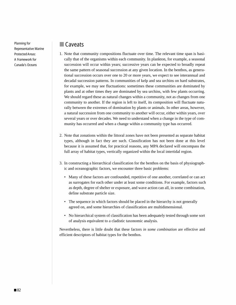
■ 82

Planning for

Representative Marine

Protected Areas:

A Framework for

Canada’s Oceans

■ Caveats1. Note that community compositions fluctuate over time. The relevant time span is basi-

cally that of the organisms within each community. In plankton, for example, a seasonalsuccession will occur within years; successive years can be expected to broadly repeatthe same pattern of seasonal succession at any given location. In the benthos, as genera-tional succession occurs over one to 20 or more years, we expect to see interannual anddecadal succession patterns. In communities of kelp and sea urchins on hard substrates,for example, we may see fluctuations: sometimes these communities are dominated byplants and at other times they are dominated by sea urchins, with few plants occurring.We should regard these as natural changes within a community, not as changes from onecommunity to another. If the region is left to itself, its composition will fluctuate natu-rally between the extremes of domination by plants or animals. In other areas, however,a natural succession from one community to another will occur, either within years, overseveral years or over decades. We need to understand when a change in the type of com-munity has occurred and when a change within a community type has occurred.

2. Note that zonations within the littoral zones have not been presented as separate habitattypes, although in fact they are such. Classification has not been done at this levelbecause it is assumed that, for practical reasons, any MPA declared will encompass thefull array of habitat types, vertically organized within the local intertidal region.

3. In constructing a hierarchical classification for the benthos on the basis of physiograph-ic and oceanographic factors, we encounter three basic problems:

• Many of these factors are confounded, repetitive of one another, correlated or can actas surrogates for each other under at least some conditions. For example, factors such as depth, degree of shelter or exposure, and wave action can all, in some combination,define substrate particle size.

• The sequence in which factors should be placed in the hierarchy is not generally agreed on, and some hierarchies of classification are multidimensional.

• No hierarchical system of classification has been adequately tested through some sortof analysis equivalent to a cladistic taxonomic analysis.

Nevertheless, there is little doubt that these factors in some combination are effective andefficient descriptors of habitat types for the benthos.

4Planning a National System ofRepresentative MPAs

4a

■ 84

Planning for

Representative Marine

Protected Areas:

A Framework for

Canada’s Oceans

Guiding Principles forDesigning a System of MPAs

■ IntroductionThis framework was developed to provide a consistent physical classification system forthe marine environment to guide the selection of MPAs. However, a classification systemalone will not be sufficient to prescribe the location and design of MPAs. Even when theseascape analysis is complete, further exercises must be carried out to determine ecologicalintegrity, to identify priority areas or special needs and to ensure that practicalities are con-sidered before proceeding to the selection of MPAs.

While the major focus of this project was the development of a framework for seascapeidentification, the integrity of areas to be identified must also be considered subsequently.In terrestrial systems, this involves concepts of ecosystem structure and function, includingaspects of size, naturalness and ecological disturbances. Separate identification guidelinesor decision rules will be needed to rank areas in terms of importance within marine systems(e.g., sites for rare and endangered species).

It should be stressed that the first stage of the process—the recognition of seascapes—is anatural one in that all areas of marine environments are included in the classification andare separated by defined physical characteristics of the environment. In contrast, the secondstage of the process—the selection of MPAs—is a more artificial process, requiring theinput of data or information according to several somewhat arbitrary criteria related to con-servation value and economic factors.

Especially in the early stages of designing an MPA network, MPAs of an almost endlesscombination of sizes and locations could sample all seascapes. Economic considerations,connectivity analyses and value judgments (e.g., about key habitat for endangered or com-mercial species) can be used in conjunction with seascape representation analysis to guidethe specific placement of MPAs. The key point is that seascape representation defines thegoal of a completed network and serves to balance common anthropocentric concerns thattend to concentrate on marine mammals and commercial fish species.

Part 4 of this report examines the criteria that can be used to move to the second stage, thatof the selection and design of MPAs.

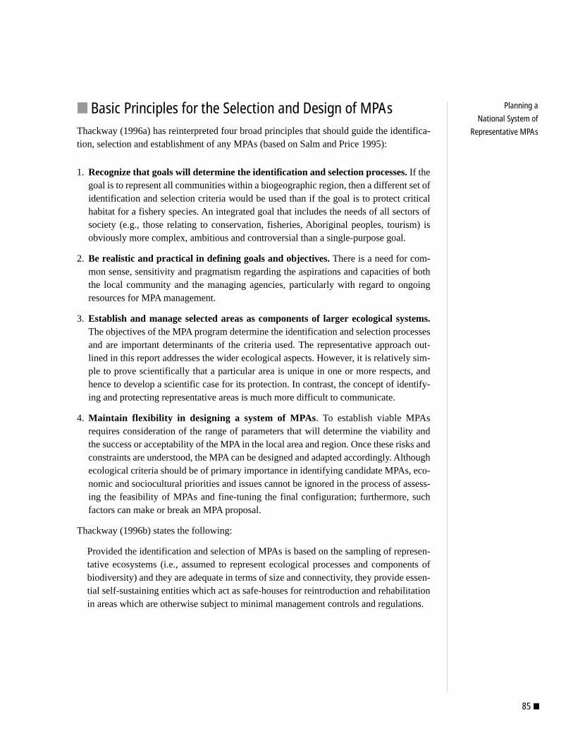
85 ■

Planning a

National System of

Representative MPAs

■ Basic Principles for the Selection and Design of MPAsThackway (1996a) has reinterpreted four broad principles that should guide the identifica-tion, selection and establishment of any MPAs (based on Salm and Price 1995):

1. Recognize that goals will determine the identification and selection processes. If thegoal is to represent all communities within a biogeographic region, then a different set ofidentification and selection criteria would be used than if the goal is to protect criticalhabitat for a fishery species. An integrated goal that includes the needs of all sectors ofsociety (e.g., those relating to conservation, fisheries, Aboriginal peoples, tourism) isobviously more complex, ambitious and controversial than a single-purpose goal.

2. Be realistic and practical in defining goals and objectives. There is a need for com-mon sense, sensitivity and pragmatism regarding the aspirations and capacities of boththe local community and the managing agencies, particularly with regard to ongoingresources for MPA management.

3. Establish and manage selected areas as components of larger ecological systems.The objectives of the MPA program determine the identification and selection processesand are important determinants of the criteria used. The representative approach out-lined in this report addresses the wider ecological aspects. However, it is relatively sim-ple to prove scientifically that a particular area is unique in one or more respects, andhence to develop a scientific case for its protection. In contrast, the concept of identify-ing and protecting representative areas is much more difficult to communicate.

4. Maintain flexibility in designing a system of MPAs. To establish viable MPAsrequires consideration of the range of parameters that will determine the viability andthe success or acceptability of the MPA in the local area and region. Once these risks andconstraints are understood, the MPA can be designed and adapted accordingly. Althoughecological criteria should be of primary importance in identifying candidate MPAs, eco-nomic and sociocultural priorities and issues cannot be ignored in the process of assess-ing the feasibility of MPAs and fine-tuning the final configuration; furthermore, suchfactors can make or break an MPA proposal.

Thackway (1996b) states the following:

Provided the identification and selection of MPAs is based on the sampling of represen-tative ecosystems (i.e., assumed to represent ecological processes and components ofbiodiversity) and they are adequate in terms of size and connectivity, they provide essen-tial self-sustaining entities which act as safe-houses for reintroduction and rehabilitationin areas which are otherwise subject to minimal management controls and regulations.

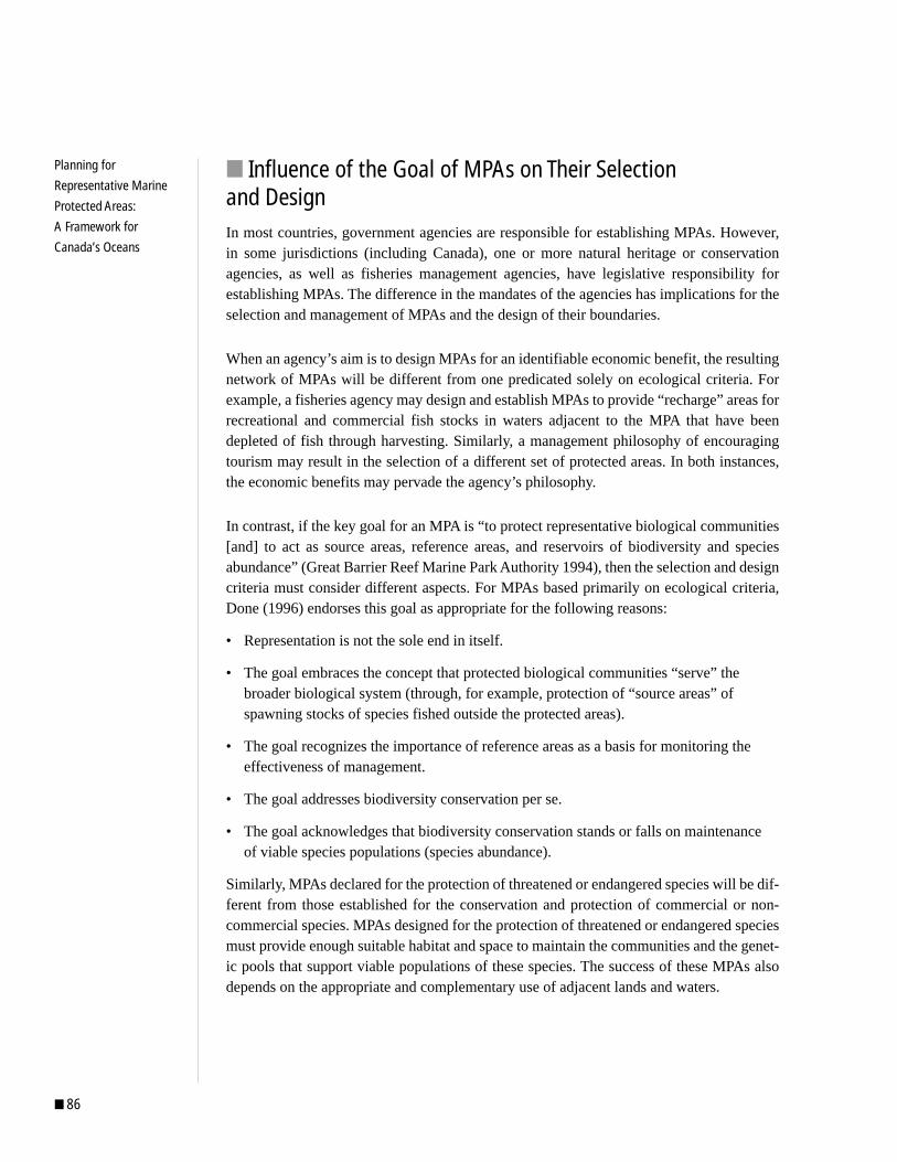
■ 86

Planning for

Representative Marine

Protected Areas:

A Framework for

Canada’s Oceans

■ Influence of the Goal of MPAs on Their Selection and DesignIn most countries, government agencies are responsible for establishing MPAs. However,in some jurisdictions (including Canada), one or more natural heritage or conservationagencies, as well as fisheries management agencies, have legislative responsibility forestablishing MPAs. The difference in the mandates of the agencies has implications for theselection and management of MPAs and the design of their boundaries.

When an agency’s aim is to design MPAs for an identifiable economic benefit, the resultingnetwork of MPAs will be different from one predicated solely on ecological criteria. Forexample, a fisheries agency may design and establish MPAs to provide “recharge” areas forrecreational and commercial fish stocks in waters adjacent to the MPA that have beendepleted of fish through harvesting. Similarly, a management philosophy of encouragingtourism may result in the selection of a different set of protected areas. In both instances,the economic benefits may pervade the agency’s philosophy.

In contrast, if the key goal for an MPA is “to protect representative biological communities[and] to act as source areas, reference areas, and reservoirs of biodiversity and speciesabundance” (Great Barrier Reef Marine Park Authority 1994), then the selection and designcriteria must consider different aspects. For MPAs based primarily on ecological criteria,Done (1996) endorses this goal as appropriate for the following reasons:

• Representation is not the sole end in itself.

• The goal embraces the concept that protected biological communities “serve” thebroader biological system (through, for example, protection of “source areas” ofspawning stocks of species fished outside the protected areas).

• The goal recognizes the importance of reference areas as a basis for monitoring theeffectiveness of management.

• The goal addresses biodiversity conservation per se.

• The goal acknowledges that biodiversity conservation stands or falls on maintenance of viable species populations (species abundance).

Similarly, MPAs declared for the protection of threatened or endangered species will be dif-ferent from those established for the conservation and protection of commercial or non-commercial species. MPAs designed for the protection of threatened or endangered speciesmust provide enough suitable habitat and space to maintain the communities and the genet-ic pools that support viable populations of these species. The success of these MPAs alsodepends on the appropriate and complementary use of adjacent lands and waters.

87 ■

Planning a

National System of

Representative MPAs

Ill-defined objectives for MPAs often result in a dilution of the conservation effort. This isa concern particularly in multiple-use MPAs that aim to accommodate all users. If the pri-mary purpose of an MPA is accepted as being a tool for the conservation of biodiversity,then ecological values must be given precedence over other values when selecting anddesigning an MPA (Inglis 1993).

In short, the mandate of the relevant agency will determine the primary purpose for devel-oping MPAs, and this, in turn, will determine the selection criteria or targets that are used toachieve the best fit with that primary purpose. Different criteria are needed for evaluatingecological values versus socioeconomic values; however, Smith and Theberge (1986) notethat ecological goals and socioeconomic goals are not mutually exclusive. Areas of highbiodiversity are often also attractive for their conservation, resource use, tourism and cul-tural values. Such links between biological values and other social and cultural values can-not be ignored and often play a critical role in the success of any MPA (Kenchington 1990).

■ 88

Planning for

Representative Marine

Protected Areas:

A Framework for

Canada’s Oceans 4bSelection Criteria for MPAs

Much of the existing literature on MPAs includes various lists of criteria that may be appliedin the identification and selection of MPAs. For example, Kelleher and Kenchington (1992)suggest selection criteria for MPAs grouped into eight categories, which have been adapted tothe seven listed in Box 4. This list has been adopted by the IUCN and is often cited.

Naturalness

• Extent to which the area has been protectedfrom, or has not been subject to, human-inducedchange

Biogeographic Importance

• Inclusion of rare biogeographic qualities or representation of a biogeographic type or types

• Inclusion of unique or unusual geological features

Ecological Importance

• Contribution to the maintenance of essentialecological processes or life-support systems(e.g., a source of larvae for downstream areas)

• Integrity

• Degree to which the area, either by itself or in association with other protected areas,encompasses a functional ecosystem

• Inclusion of a variety of habitats

• Inclusion of habitat for rare or endangeredspecies

• Inclusion of nursery or juvenile areas

• Inclusion of feeding, breeding or rest areas

• Inclusion of rare or unique habitat for anyspecies

• Preservation of genetic diversity

Economic Importance

• Existing or potential contribution to economic

value (e.g., recreation, subsistence, use by tradi-tional inhabitants, appreciation by tourists andothers, use as a refuge nursery area or source ofsupply for economically important species)

Social Importance

• Existing or potential value to the local, nationalor international communities because of its heritage or historical, cultural, traditional,aesthetic, educational or recreational qualities

Scientific Importance

• Value for research and monitoring

• International or national importance

• Potential to be listed on the world or a nationalheritage list; to be declared as a biospherereserve; to be included in a list of areas of international or national importance; or to bethe subject of an international or national conservation agreement

Practicality or Feasibility

• Degree of insulation from external destructiveinfluences

• Social and political acceptability and degree of community support

• Accessibility for education, tourism and recreation

• Compatibility with existing uses, particularly by local people

• Ease of management and compatibility withexisting management regimes

Box 4. PROPOSED CRITERIA FOR ASSESSING THE SUITABILITY OF AN AREA AS AN MPA

89 ■

Planning a

National System of

Representative MPAs

To achieve a representative network of MPAs, the selection of sites could follow these steps:

1. Systematically classify all marine habitat types using a consistent framework.

2. Systematically choose a network of candidate MPAs using the framework to incorporatethe representative patterns characteristic of each seascape.

3. Further assess the candidate MPAs, ensuring, wherever possible, that other important,unique or distinctive features are incorporated and that other non-ecological criteria (e.g.,socioeconomic aspects) are considered. If, for valid or critical reasons, the candidateMPAs initially chosen are deemed inappropriate, then similarly assess other candidateMPAs until acceptable MPAs and, ultimately, a network of representative MPAs are identified.

4. Develop appropriate zoning for the MPAs chosen to ensure that all the essential elements of the ecological diversity of the marine communities remain adequately protected in perpetuity.

Figure 3 illustrates three options for designing a network of MPAs in a natural region, basedonly on seascape representation (i.e., the first two steps above).

Currently, most marine management agencies identify and select MPAs by a manual scoringbased on a set of selection criteria (such as that listed by Kelleher and Kenchington 1992) oran iterative evaluation of similar criteria. Research by Pressey and Nicholls (1989) on thevalue of such scoring of selection criteria compared with systematic interactive computer-based algorithms showed that scoring methods were less efficient than interactive computer-based approaches. The major advantages of such computer-based approaches are that theyprovide flexibility for testing and comparing different design scenarios (or reserve options)and for comparing the costs and benefits of these different reserve options. However, not allagencies have access to the detailed GIS data required to use such methods.

When identifying and selecting MPAs, we need to consider the following points:

• If we are to trying to choose a set of MPAs that represent the marine biodiversity withinan area, we will need to use a systematic ecological basis for the selection process.Decisions should be made within the context of an entire area, rather than by consideringonly small locations about which more details are known.

• Many agencies and jurisdictions apply these criteria largely in isolation of neighbouringjurisdictions and even agencies within the same jurisdiction. There is, therefore, a need todefine and apply consistent and appropriate criteria and guidelines for the identificationand selection of individual MPAs.

• Where there is a multitude of identification and selection criteria, it may be difficult torate them all equally.

■ 90

Planning for

Representative Marine

Protected Areas:

A Framework for

Canada’s Oceans

Figure 3. CONCEPTUAL OPTIONS FOR A REPRESENTATIVE NETWORK OF MPAs

IN A MARINE NATURAL REGION

Option 1

No representation of seascape A

Moderate representation of seascape B

Partial representation of seascape C

Partial representation of seascape D

Assessment

Natural region partially represented.

Option 3

Adequate representation of seascapes A, B,

C and D

Assessment

Natural region adequately represented. This is

the best option for representation because

the candidate MPAs adequately represent

each of the seascapes and have connections

to surrounding seascapes.

Option 2

Partial representation of seascape A

Adequate representation of seascape B

Moderate representation of seascape C

Adequate representation of seascape D

Assessment

Natural region moderately represented.

�y��yy�y�y��yy��yy

�y��yy��yy

Source: Adapted from Kavanagh and Iacobelli 1995.

Legend

��yy

Seascape A

Seascape B

Seascape C

Seascape D

Marine natural region

Possible MPA boundary

91 ■

Planning a

National System of

Representative MPAs4cEcological Principles andCriteria for Designing a Systemof MPAs

When designing representative MPAs, we must consider additional ecological design crite-ria. The environmental connectivity of areas, the appropriate shape and size of a reserve, thelevel of natural heterogeneity, the ecological vulnerability and the need for replication areimportant considerations. There is no known order in which these ecological criteria shouldbe applied; rather, an iterative approach is recommended when developing an MPA propos-al. Furthermore, some criteria will be more critical than others, depending on the specificlocation or the circumstances.

A new principle also enters the process when proceeding from seascapes to MPAs. Whereasour analysis of seascapes was conducted at the community level, to proceed to the MPAlevel, we must take into account processes at the population level. In particular, we need toexamine what populations (e.g., migrant species) we may have missed at the communitylevel and how they exploit the environment spatially.

■ Reserve SizeThe issue of whether a candidate protected area will be adequate in size is important, partic-ularly in the case of fragmented or highly modified seascapes or in areas that are undergoingdegradation. In most cases a precautionary approach would suggest that larger rather thansmaller areas should be chosen and that strictly protected areas should have appropriatebuffer zones. It is also preferable that strong conservation management principles be appliedas much as possible outside and surrounding the areas of ecological importance.

The size of a candidate MPA may be influenced by the proposed management type (see thediscussion of reserve management type below). Consequently, while an ecological basisshould be the primary determinant of the size of a reserve, its future management may alsodetermine the area likely to be socially and politically acceptable. In all cases, stronginvolvement of user groups and the community is required in setting up the system for it tobe accepted and effective (Benzie 1996).

The principle of a buffer zone protecting a core site from human impacts is well establishedand, wherever possible, should be applied to all MPAs. However, since coastal and continen-tal-shelf environments are often linear in nature and subject to established heavy use, buffer-ing, although desirable, may be impracticable in some cases (Kelleher and Kenchington1992).

■ 92

Planning for

Representative Marine

Protected Areas:

A Framework for

Canada’s Oceans

From an enforcement perspective alone, MPAs should, as a general rule, be large and man-ageable rather than small and highly dispersed with complex zoning configurations.

If the goal of an MPA is primarily to protect a specific marine species, Shepherd and Brown(1993) maintain that reserve size must be determined in relation to the internal dynamicsand size of the metapopulations in question. Small metapopulations will require the conser-vation of a much larger fraction of those metapopulations conserved than would largemetapopulations with many interconnecting local populations. For example, SouthAustralia’s only long-term abalone reserve (West Island Reserve) failed to protect ametapopulation because it was too small and enforcement was inadequate for preventingpoaching.

■ Reserve NetworksBallantine (1991) stresses the need to consider the following issues when deliberating overreserve size and number:

• Many marine populations have dispersive phases and reproduction is decoupled fromrecruitment. It is rarely possible to identify the parental origins of any particular popula-tion or to specify which area(s) the offspring of one population will recruit. In any case,the answer is likely to be different for each species (with different reproductive seasonsand length of planktonic phase) and often different in the same species for differentyears (owing to current variations, whether random or systematic). It follows, therefore,that a well-designed network of reserves (including spaced replicates) is much moreeffective in promoting recruitment (including to other reserves) than a few large ones.

• Present knowledge of the interactions between different marine habitats and communi-ties is sufficient to show that these are common and self-sustaining, but it is not enoughto specify the size of area that would be self-sustaining. Consequently, while reservesshould contain as many representative habitats as possible, this should not override theprinciple of a network.

• The minimum area of biologically useful marine reserves may be as small as a fewsquare kilometres (except where the entire system itself is smaller, e.g., a small estuary).However, in all cases, the addition of adjacent areas is highly desirable, since importantinteractions with such adjoining areas are very likely.

Central to the concept of a network of MPAs is the understanding that protected areasshould operate as an interconnected group or system. The main requirement, then, is todesign protected areas so that species can move readily from one reserve to another; this isnot necessarily done by providing strips of habitat connecting larger habitat areas, butinstead by providing habitat that maintains broad patterns of movement (Schmeigelow1997). Other management strategies, such as temporal regulation of human activities, mayalso be critical for species movement or recruitment. Therefore, the following must be con-sidered when configuring reserves:

93 ■

Planning a

National System of

Representative MPAs

• The type of movements important for population persistence (e.g., juvenile and adultdispersal, foraging, seasonal migration)

• The spatial and temporal scale of these movements

• The natural levels of connectivity in the system

• The broader context in which the MPAs are located (i.e., the surrounding managementregimes)

■ Reserve ConnectivityDone (1996) explains that for MPAs to act as source areas and reservoirs of biodiversityand species abundance, they need connectivity. A good source area will be one chosen tomaximize the probability that the propagules emanating from it will actually succeed. Thatis, they have a higher than average probability of arriving at an appropriate habitat (eitheranother MPA or not) while still viable (Kelleher et al. 1994).

Done (1996) continues:

Potential protected areas will vary in the degree to which they are self-seeding and thedegree to which they rely on outside areas for replenishment of populations depleteddue to natural attrition, harvesting or habitat degradation. There are two bases for thisvariability. First, there is great variability in the buoyancy and capacity for activeswimming of the planktonic stages of different biota. Second, the current regimes towhich the planktonic stages will be exposed are regionally variable.

The following lists a number of relevant aspects for connectivity if an MPA is specificallydesigned for a particular target species (based on Noss 1995):

1. Mobility or dispersal of the target species including the following:

• Species-specific habitat preferences for movement

• Dispersal distance or scale of resource utilization

• Rate of movement or dispersal

2. Other ecological characteristics of the target species (e.g., preference for a particularstructural feature; feeding requirements; mortality risks)

3. Seascape context: structural characteristics and the spatial pattern of the seascape

4. Distance between patches of suitable habitat

5. Interference from humans and predators

■ 94

Planning for

Representative Marine

Protected Areas:

A Framework for

Canada’s Oceans

Computer simulations based on best available models of underlying oceanographic and bio-logical bases have been used both to optimize site selection based on the best use of presentknowledge (e.g., James et al. 1996) and to highlight the needs for filling gaps in data andunderstanding. However, the interest in the role of source and sink sites in determiningrecruitment and, therefore, their inclusion in MPAs may belie our actual capacity to identifythese effectively, particularly as these factors vary from organism to organism and fromtime to time. Nevertheless, although a site may not be an important sink or source, it maystill be important in terms of its representativeness.

■ Reserve ShapeA considerable number of theoretical approaches to the optimum shape for reserves exist;given the problems of the impacts associated with edge effects in terrestrial systems, theoptimum shape for a reserve in such systems is frequently believed to be circular. However,because of the fluid and mobile nature of the marine environment, the issues associated withedge effects on boundaries are not as relevant as they are in terrestrial reserves. Further-more, the optimum shape for marine reserves is not the circular shape depicted in many ofthe theoretical texts (i.e., a core area surrounded by concentric circles of buffer). Rather, theoptimum shape for an MPA is dependent on criteria similar to those defined for the designof networks—such as juvenile and adult dispersal, foraging, seasonal migration, naturallevels of connectivity— and the surrounding management regime.

The resulting optimum shape for an MPA (unless it is large and encompasses a broad area)will depend on the purpose of the MPA. If the goal is to maximize protection of a singlespecies, the MPA should be parallel to the coast and/or the prevailing current. If the goal isto maximize biodiversity in the MPA, a cross-shelf configuration may be optimal. However,a number of practical aspects require consideration when determining the configuration ofan MPA boundary. Spatial boundaries are relevant to only some facets of integrated man-agement of marine biodiversity, and lines on maps have limited validity when it comes toopen waters, particularly if those lines are based on seabed features.

Once the ecological determinants have been applied to a candidate area, the actual shape ofa preferred MPA, as well as the management regimes within the MPA, can be determined ona pragmatic and socioeconomic–legal basis. For practical reasons, it is often necessary toalign ecological boundaries with more distinguishable human-related features. Whereverpossible, these boundaries should encompass the underlying ecological boundaries. Manypragmatic considerations can influence reserve shape:

• Recognizable boundary features and markers

• Ease of access

• Existing levels and types of uses

• Potential in terms of what might be legally declarable

• Potential in terms of what might be better for enforcement and surveillance

95 ■

Planning a

National System of

Representative MPAs

■ Reserve Management TypeWhether a small no-take area is better (from a conservation standpoint) than a larger multiple-use MPA will obviously depend on the specific circumstances. However, given that marineecosystems are relatively large, fluid and interconnected, it follows that a network of reserves(including spaced replicates) could be more effective in promoting recruitment (including toother reserves) than would be a few large reserves (see discussion of networks above). Morereserves and protected areas foster biological links that increase these advantages even fur-ther. For example, a few unexploited marine reserves are unlikely to have any general orwidespread effects, however large the difference between their state and that of adjacentexploited areas. In contrast, a network of such reserves is likely to have such effects, even ifwe do not know, and may never know, which parts of the network achieved which results.

Many people consider the management model based on a large multiple-use MPA with zon-ing (e.g., the Great Barrier Reef Marine Park [GBRMP]) to be advantageous in that it canprovide for an overall level of protection and for consistency in planning and management, aswell as enable strategically placed, small, highly protected core areas. Such a model can serveboth to preserve biodiversity and to help sustain ecosystem integrity and allow the use ofmarine resources within the larger managed area. Pressey and McNeill (1996) give the fol-lowing argument in favour of multiple-use areas:

The multiple use model allocates activities through zoning and is considered more effec-tive than small, isolated, highly protected areas for several reasons:

1. Ecologically, it recognizes the temporal and spatial scales at which marine ecosystems operate;

2. Practically, it is easier to manage and potentially buffers and dilutes impactsof activities in areas adjacent to strictly protected areas; and

3. Socially, it helps to resolve and manage conflicts in the use of natural resources.

However, few MPAs of a size comparable to the GBRMP have been declared to obtain max-imum benefit as outlined by Pressey and McNeill (1996).

■ Reserve Replication and RedundancyAny large disturbance in marine systems, whether natural (e.g., cyclones) or man made (e.g.,oil spills), can destroy the very qualities of an MPA—its intrinsic values as well as its con-nections—for which it was chosen. The need to plan for such disturbances is, therefore, wellaccepted in the field of protected area management. However, unlike in terrestrial systems,where the recommended goal is reservation of areas large enough to accommodate any dis-turbance, in marine systems replication or redundancy is considered a more prudent strategy.MPAs should, therefore, be configured to minimize the likelihood that the entire representa-tion of a seascape would be degraded at any one time by natural or human disturbance.

■ 96

Planning for

Representative Marine

Protected Areas:

A Framework for

Canada’s Oceans

For example, even if one metapopulation were to suffer decline due to disease, overhar-vesting or habitat destruction, the entire stock would be less at risk if other reserves existedto protect other metapopulations (provided these are unlikely to all suffer the same disasterat the same time). Essentially, the more MPAs that are declared, the greater the chance of avariety of benefits accruing.

Seascapes and candidate MPAs generally convey no information about the relative value orprotection priority for each seascape. Pressey and McNeill (1996) therefore recommend aspecific approach:

More information on the relative value of planning units can be conveyed by analysesthat show the irreplaceability of areas (Pressey et al. 1994). These analyses produce amap of all the individual areas being considered for reservation, indicating two things:

• The likelihood that any particular planning unit will be needed as part of a represent- ative reserve system

• The extent to which the options for achieving a representation goal will be reduced if the planning unit is made unavailable for protection

Irreplaceability puts a number on the obvious fact that there are no options for reservingsome units but many options for reserving others. Some units are totally irreplaceable,either because they contain unique features or because they contain so much of one ormore features that the reservation goal can no longer be achieved if the unit is notreserved. Other units are replaceable to varying degrees. A map of irreplaceability in aregion is therefore a map of options for developing a representative reserve system.

Where the goal is to conserve biodiversity, it is necessary to identify and select priorityareas on the basis of agreed biodiversity values.

4d

97 ■

Planning a

National System of

Representative MPAs

Other Selection Criteria for MPAs

Decisions about whether any particular coastal or marine areas should be conserved, devel-oped or left as they are ultimately hinge on arguments regarding the relative merits of eco-logical goals compared with socioeconomic goals. Whether to give greater weighting toecological goals or to socioeconomic goals (including the decision whether to establish aconservation reserve) is primarily a political and social process like any other public policydecision.

In developing options for MPAs, planners initially need to define a number of candidateareas using ecological principles that recognize representativeness and that consider addi-tional ecological determinants such as unique and special areas. However, planners alsoneed to recognize that the decisions on final MPA configurations (e.g., locations, bound-aries, size, type) will necessarily involve consideration of a much wider range of selectioncriteria and other determining factors. Consequently, once the above ecological criteriahave been applied and a number of candidate MPAs have been identified, the extent of theirboundaries must be optimized. To do this, a number of subordinate criteria must be consid-ered; such economic, social, political, legal and cultural considerations are discussedbelow. However, it is important to realize that some of these additional criteria may also actto constrain the development of a representative system of MPAs by providing reasons whyan area should not be included in an MPA.

It is rare that planners or managers have the luxury of determining an ideal boundary orconfiguration for any form of conservation reserve or MPA. Rather, the precise locationand boundaries of an MPA are usually the collective decision of park planners, politiciansand the public (Ballantine 1991) and are not based strictly on any scientific formula orchecklist. Science may inform the debate and influence the outcome, but it will not be alonein making the final decision. Ultimately, there must be enough public and user support forMPAs to overcome the natural resistance of some special interest groups and decision mak-ers so that they change the status quo.

In evaluating candidate MPAs, the approach used by Parks Canada in coordinating work-shops of experts to provide the most accurate and current information on a particular loca-tion (e.g., Mercier 1995) is valuable, particularly for determining unique and special areasthat also need to be considered when evaluating MPA proposals. Ideally, planners will useiterative approaches using GIS techniques, in conjunction with expert opinion.

At this stage, a review of the benefits of no-take MPAs versus multiple-use MPAs is appro-priate.

■ 98

Planning for

Representative Marine

Protected Areas:

A Framework for

Canada’s Oceans

MLSS (nd) summarizes some of the social and managerial benefits of harvest refugia (no-take MPAs) and multiple-use MPAs (noting that these can be used in complementary fash-ion).

■ Benefits of No-Take MPAs 1. Fairness and equity to user groups: No single group is favoured at the expense of oth-

ers, as harvest refugia prevent use by all fisheries.

2. Simplified management and enforcement: Because harvesting is totally prohibited,management and enforcement are simplified. Violations can be detected easily by fisheries officers, volunteer wardens or the public. Similarly, it is easier to communi-cate the no-take regulations to all visitors.

3. Community involvement: Because harvest refugia can be relatively small, coastal communities can identify areas that need protection and request legal protection forthose areas by governments.

4. Research and monitoring: No-take zones can be used to establish a baseline by which to assess change in unprotected areas.

■ Benefits of Multiple-Use MPAs 1. No-take zones: More often than not, some zones within a multiple-use MPA are likely

to be designated as no-take zones.

2. Integration of human activity and conservation: Innovative solutions can dispel themyth that conservation and resource use are incompatible.

3. Adaptive management: Zones can be reviewed on a regular basis, allowing managersand scientists the flexibility to respond to changes in human activity and the environ-ment (e.g., Great Barrier Reef Marine Park).

4. Development of management partners: As human activities are integrated in multiple-use MPAs, coastal communities and stakeholders become important long-term partnersin planning and management.

5. Research and monitoring: Whereas no-take zones establish control sites for research,multiple-use MPAs can provide opportunities for researching and monitoring the sus-tainable use of an area.

99 ■

Planning a

National System of

Representative MPAs

■ Airspace Above an MPAWhen most MPA proposals are evaluated, virtually all consideration is given to the marineaspects alone (pelagic and benthic). Little consideration is given to the airspace above anMPA, yet this is often a critical component for successful management of the MPA. Forexample, if the conservation of whales is a priority within an MPA and there are no controlsover aircraft, such as controls on minimum flying heights, then aircraft can have majoreffects on such species, particularly if whale watching becomes a major tourist industry.

The use of hovercraft in sensitive areas today can have major effects if such use is not man-aged, yet it could be argued that hovercraft are operating over rather than within the marineenvironment. Furthermore, with rapid advances in technology, it is likely that in less than adecade some vessels will probably be surface assisted and extremely fast (i.e., operate morelike extremely low-flying aircraft with the ability to cover huge distances quickly and easi-ly). Consequently, an MPA should also extend some distance above the water surface; anexample of airspace being part of an MPA is the Great Barrier Reef Marine Park, whereprotected airspace has been declared up to a height of 3000 feet above sea level. While thenavigation of most aircraft is unimpeded in most zones of the park, this regulation providesmanagers with the ability to apply controls when and where necessary.

■ 100

Planning for

Representative Marine

Protected Areas:

A Framework for

Canada’s Oceans 4eSpecial Areas

A representative approach to MPAs specifically does not identify special or unique sites forprotection. Rare species and special sites need to be dealt with separately from ecological-ly representative sites.

The Oceans Act (section 35) has provision for “the conservation and protection of uniquehabitats.” Other possible examples of unique areas cited in the DFO (1997) discussionpaper include “breeding areas, spawning areas, nursery areas, genetic ‘seed banks,’ ‘rarespecies’ habitats, polynyas, estuary zones, tidal flats, kelp forests, offshore banks, perma-nent or seasonal upwelling or mixing areas, deep sea vents, sea mounts, salt marshes, ormarine mammal habitat.” Note that some of these areas are already captured at the commu-nity level by the delineation of seascapes; others, predominantly those at the populationlevel, are not.

People generally are more likely to see the point of special status for special or distinctareas than they are to comprehend restrictions on existing uses of representative areas. It istherefore critical that the scientific values of representative MPAs be explained.

An example of a special community that warrants protection is given by McNeill (1996).McNeill discusses some of the biological characteristics of sea-grass beds, citing the designof various existing MPAs that in no way reflect an understanding of the critical processesstructuring the sea-grass systems (e.g., spatial and temporal variability of species, recruit-ment, seasonality, life cycle requirements). McNeill justifies protecting the maximum areaof sea-grass beds within estuaries and argues that their protection should override otherconsiderations in the design of MPAs for the following reasons:

1. Maintenance of seagrass beds and their associated communities is critical for the long-term sustainability of coastal ecosystems.

2. Seagrass habitats, located within estuaries, are more vulnerable to damage and destruction from physical disturbance and adjacent land use than many other marine habitats.

3. Seagrasses lack resilience to disturbance; once destroyed, seagrass beds do not readily recolonise.

101 ■

Planning a

National System of

Representative MPAs

Many other special or unique areas might be important to include in a system of representative MPAs:

• Habitat for rare or threatened species

• Source areas for recruitment and replenishment

• Important corridors for migratory species

• Feeding, breeding or resting areas

• Nursery, juvenile or spawning areas

• Areas of unusually high species richness

• Natural or unspoiled areas

• Unique or unusual geological features

• Benchmark and reference sites

• Areas of cultural or traditional significance

A well-planned system of MPAs can be representative of all habitat types and still capturea wide range of these areas of special importance.

■ 102

Planning for

Representative Marine

Protected Areas:

A Framework for

Canada’s Oceans 4fSummary: Guiding Principlesfor Choosing Individual MPAs

MPAs will often be chosen according to different ecological, economic and cultural priori-ties. However, there are some principles that can be used to guide the selection and designof all MPAs to maximize conservation gains.

1. MPAs should be chosen in relation to marine representation and not solely in relationto themes or species that are high in public profile.

2. The precautionary principle should be adhered to, which means that lack of scientificcertainty about such aspects as where MPAs should be located, how large they shouldbe or how many are needed should not be used as a reason for not establishing MPAs.

3. Information about special or unique biological communities, habitats or species, whereavailable, should be used to enhance the selection of MPAs.

4. The following guidelines should be followed when determining the management planto ensure that MPAs maintain ecological integrity:

• Natural processes and disturbance regimes should be allowed to continue.

• Viable populations of native species should be maintained in natural patterns of abundance and distribution.

• Species dispersal should be maintained by functionally linked, core no-take areas.

5. No-take MPAs, or no-take zones within an MPA, should be established to provide ecological benchmarks and allow for naturally functioning population interactions.

6. The size and configuration of MPAs should be sufficient to do the following:

• Incorporate a diversity of marine enduring features.

• Maintain the long-term integrity of natural communities.

• Include both resident flora and fauna, as well as relevant migratory species.

7. As far as practicable, representative samples of all communities in the MPA should beincluded within one or more no-take zones.

8. Significant breeding or nursery sites should be included either within no-take zones orwithin an appropriate seasonal closure (that is, given a high degree of protection oneither a permanent or a seasonal basis).

103 ■

Planning a

National System of

Representative MPAs

9. Single zonings or regulatory provisions should surround areas with a discrete geo-graphical description (i.e., if at all possible, single islands or reefs should not havemultiple zonings or split zonings, which can have major implications in terms of public confusion and enforcement issues).

10. In the pattern of zones within a multiple-use MPA, sudden transitions from highlyprotected areas to areas of relatively little protection should be avoided. The conceptof buffering should be applied wherever possible.

11. In the selection phase, all available information on human-use patterns, economic andsocial values, and Aboriginal cultural values should be considered.

12. Some habitat types can be sampled equally well by MPAs at a number of differentlocations. Furthermore, different configurations of a candidate area can sometimessatisfy similar ecological criteria. In these cases, the option that imposes the leastshort-term and long-term cost (where cost does not refer only to monetary value) to nearby communities and stakeholders should be adopted.

■ 104

Planning for

Representative Marine

Protected Areas:

A Framework for

Canada’s Oceans 4gConclusion

WWF Canada’s goal is the completion of a national network of MPAs by the year 2010.The goal is not to create a system for the sake of having a system; rather, the goal is one ofa suite of essential actions that will help ensure the health of our oceans and Great Lakes,along with the sustainable use of areas outside MPAs and the proper regulation of pollu-tants and toxins.

A system of MPAs must be more than an ad hoc collection of sites with no overarchingrationale or protection standards. Conservation of biodiversity will not be achievable with-out a network of well-planned and scientifically based protected areas, with strong protec-tion standards, as part of good overall oceans management.

The framework developed here is meant to help provide an ecologically sound, consistentand transparent method to define the overall goal and to generate and assess candidate sites.Furthermore, this framework uses physiographic and oceanographic features that are, forthe most part, readily available and that describe community diversity at a broad scale. Noone knows with certainty how many MPAs are needed in Canada, where exactly theyshould be located or how large they should be to ensure conservation of our marine biodi-versity. However, we don’t have the luxury of waiting until all the information is at handbefore we begin. We must make decisions based on the best available knowledge andincorporate new information as it becomes available. The sooner we begin and the morepeople that are involved, the more effective the system of MPAs will be.

Glossary

■ 132

Planning for

Representative Marine

Protected Areas:

A Framework for

Canada’s Oceans

Glossary

abiotic. Without life.

abyss. The great depths of the oceans, usually considered to be depths of 2000 to 6000 metres, aregion of low temperatures, high pressure and an absence of sunlight.

algae. The simplest plants; may be single-celled (such as diatoms) or quite large (such as seaweeds). Live in salt or fresh water.

anadromous. Of or relating to migratory fish species, such as the Atlantic and the Pacificsalmon, that spawn in fresh water but spend most of their lives in salt water.

aphotic zone. The deepest part of the water column, where light does not penetrate.

archipelago. A group of islands.

assemblage. A neutral substitute for “community” but implying no necessary interrelationshipsamong species; also called species assemblage.

baseline. The low-water line along the coast as marked on large-scale charts officially recog-nized by Canada; used for measuring the breadth of the territorial sea, except where the coast-line is indented or where a fringe of islands is in its immediate vicinity, in which case straightbaselines join appropriate points.

bathymetry. The measurement of depth in oceans, seas and lakes.

bathypelagic zone. The dark, deep part of the water column (1000–2000 m) below the euphotic(well-lighted) zone and mesopelagic (poorly lighted) zone but above the abysso-pelagic zone.

benthic. Of or relating to organisms, both plant and animal, that live on the substrate under abody of water; those living on the ocean floor are the epifauna, while those living within thesediments are the infauna.

benthos. The bottom of a sea or lake; the collection of organisms living on or in sea or lake bottoms.

biocenosis. An assemblage of species characteristically found together. Relationships to habitattype are not specified. A modern conception of this older term might be the biological recurrent group.

biodiversity. The diversity of life, often discussed in terms of three hierarchical levels: geneticdiversity (diversity within species), species diversity (diversity among species) and ecosystemdiversity (diversity among ecosystems). Also called biological diversity.

biogeographic region. A complex area of land and/or water composed of a cluster of interactingecosystems that are repeated in similar form throughout. Biogeographic regions vary in size,with larger regions found where areas have more subdued environmental gradients.

133 ■

Glossarybiome. A major regional or global biotic community characterized chiefly by the dominantforms of plant and animal life and the prevailing climate.

bioregion. An area of land and/or water whose limits are defined by the geographical distribu-tion of biophysical attributes and ecological systems.

biosphere. That part of the earth system (air, water and rock) that supports life.

biota. The organisms in a specified area.

biotic. Living or having to do with life or living organisms.

biotone. A zone of transition between core provinces. Biotones are not simply “fuzzy” bound-aries but represent unique transition zones between the core provinces. Biotones are uniquesystems and need to be recognized for their contribution to explaining the marine environ-ment.

biotope. An assemblage of species generally found together in a characteristic habitat.

catadromous. Of or relating to migratory fish species, such as eels, that breed in salt water butspend most of their lives in fresh water.

cetacean. Member of the order Cetacea, primarily marine mammals (a few freshwatercetacean species exist), with nostrils on the top of their heads. Whales, dolphins and porpoises are cetaceans.

coastal waters. Both benthic and pelagic ecosystems that are influenced substantially by theland.

community. A group of species that generally are assumed to be interdependent (though this isoften not demonstrated). The term can be used in a variety of hierarchies. Communities atlarger scales can be progressively subdivided, such as spatially, taxonomically and trophi-cally, to finer scales: for example, the North Atlantic plankton community, the Fucus com-munity of rocky shores and the zooplankton community.

contiguous zone. A zone that adjoins the territorial sea and over which Canada may exercisecontrol, such as enforcing laws relating to customs and immigration. Canada’s contiguouszone extends 24 nautical miles from the baseline.

continental margin. The submerged prolongation of the land mass of Canada consisting ofthe seabed and subsoil of the continental shelf, slope and rise but not the deep ocean floor.

continental shelf. The seabed and subsoil of the submarine area that extends beyond the terri-torial sea throughout the natural prolongation of the land territory to the outer edge of thecontinental margin where it is beyond 200 nautical miles, or 200 nautical miles where themargin is less than that distance; generally, the most productive part of the sea.

continental slope. The descent from the continental shelf to the deeper (abyssal) depths.

crustacean. Any of various predominantly aquatic arthropods of the class Crustacea, includinglobsters and crabs, characteristically having a segmented body, a chitinous exoskeleton andpaired jointed limbs.

■ 134

Planning for

Representative Marine

Protected Areas:

A Framework for

Canada’s Oceans

demersal species. A fish (also called groundfish), cephalopod or crustacean that spends itstime on or near the bottom, although it can swim.

diadromous. Of or relating to species that migrate between fresh water and salt water regular-ly during their life cycle.

dysphotic zone. The part of the water column, below the euphotic zone, that receives low lev-els of sunlight but insufficient to support plant growth.

ecoregion. In terrestrial ecological land classification terminology, an area of land “character-ized by distinctive ecological responses to climate as expressed by vegetation, soils, waterand fauna” (Wickware and Rubec 1989). Ecoregions are one of several hierarchical levelsof classification and are mappable at scales of between 1:1 million and 1:3 million.Ecoregions are the fundamental units of representation for terrestrial and marine gap analy-sis.

ecology. The scientific study of the interaction between living things and their environment.

ecosystem. A definable part of the biosphere consisting of several interacting communities; itreceives inputs from the surrounding land, water and atmosphere, and may create outputs toother locales. A much misused term, it is not synonymous with “habitat” or “community.”

echinoderm. Any of numerous radially symmetrical marine invertebrates of the phylumEchinodermata, which includes the starfishes, having an internal calcareous skeleton andoften covered with spines.

endangered species. A species whose global population has been reduced to a level that isclose to or beneath the sustainable level for that species. Since they are in imminent dangerof becoming extinct, endangered species are protected under laws recognized by manycountries.

enduring feature. A landscape element or unit within a natural region characterized by rela-tively uniform origin of surficial material, texture of surficial material and topography orrelief. See also marine enduring feature.

epibenthic. Living on the surface of bottom sediments in a water body.

estuary. An ecosystem in which a river or stream meets the ocean; characterized by intermedi-ate or variable salinity levels and often by high productivity.

euphotic zone. The upper part of the water column that receives sufficient light to allow plantgrowth.

eutrophic. Of or relating to waters rich in plant nutrients that support high rates of plantgrowth.

exclusive economic zone (EEZ). An area beyond and adjacent to the territorial sea, subject tothe specific legal regime of Canada, under which the rights and jurisdiction of Canada andthe rights and freedoms of other coastal states are governed by the relevant provisions ofthe United Nations Convention on the Law of the Sea.

fauna. A broad term for animal life.

135 ■

Glossaryfetch. The distance travelled by unobstructed wind or waves.

fjord. A long, narrow, deep inlet of the sea between steep slopes. Also spelled “fiord.”

flora. A broad term for plant life; the plants of a particular area, region or time.

gap analysis. A technique designed to evaluate existing protected areas with regard to theirrepresentativeness (of marine ecosystems), to determine what further representation isrequired and to identify where those additional protected areas are located.

gyre. A circular ocean current.

habitat. A space with definable physical characteristics and limits within which organismslive.

hadal. Pertaining to depths of the ocean greater than 6000 metres.

indigenous. Of or relating to any of the Aboriginal peoples of a particular region.

inshore. Of the near coastal waters extending from the coastline and estuaries out to 3 nauticalmiles.

intertidal zone.The area between the high-water mark and low-water mark that is submergedat high tide and exposed at low tide.

invertebrate. An animal without a backbone or spinal column (i.e., not vertebrate).

kelp. Any of various brown, often very large seaweeds of the order Laminariales.

littoral zone. See intertidal zone.

marine. Of or relating to the sea; native to, inhabiting or formed by the sea.

marine ecological principles. Statements designed to guide the development and implementa-tion of a marine representation framework and methodology. The principles use marineecological attributes along with representation, mapping and ecological integrity require-ments for a network of marine protected areas.

marine enduring feature. An abiotic marine ecological attribute that is considered most representative of marine ecosystems, is observable and measurable, and exerts an organizing influence on the distribution and diversity of marine species and communities. Such features can be used to identify major representative units for the purposes of classification, mapping and gap analysis.

marine protected area. An area set aside under legislation to protect marine values.

mollusc. A member of a large phylum of invertebrate animals characterized by soft, unsegmented bodies and usually having a calcareous shell.

natural region. In the ocean, a broad oceanographic and biophysical area characterized by particular water-mass characteristics and sea-ice conditions.

■ 136

Planning for

Representative Marine

Protected Areas:

A Framework for

Canada’s Oceans

nekton. An aquatic organism, such as fish and krill (euphausiids), that can swim powerfullyenough to move against currents.

neritic. Pertaining to the water column overlying the continental shelf.

network. A group of sites related to each other or interacting on the basis of known or specifiedcriteria so as to form a collective unity. Parts of the network should relate to or complementeach other in some way.

neuston. The diversity of minute or microscopic organisms that inhabit the surface layer of a bodyof water.

niche. The range of environmental variables (such as temperature, salinity, nutrients) within whicha species can exist and reproduce. The preferred (or fundamental) niche is the one in which thespecies performs best in the absence of competition or interference from extraneous factors.

nonphotic zone. The part of the water column where plant growth cannot occur. This zoneincludes the dysphotic zone (where light is insufficient for photosynthesis) and the aphoticzone (where there is no light at all).

offshore. Of the area of the exclusive economic zone extending from the border of the territorialwaters to the limit of Canada’s international marine boundary.

pelagic. Of, relating to or living in the water column of seas and oceans (as distinct from benthic).

phytoplankton. Microscopic free-floating algae that drift in sunlit surface waters.

pleuston. Organisms that float on the surface of the sea.

plankton. Small or microscopic aquatic organisms that are suspended freely in the water column;they drift passively and cannot move against the horizontal motion of the water.

polynya. An area of open water surrounded by sea ice.

precautionary principle. The guiding ecological principle that maintains that, when consideringwhich activities to permit, only those that have been demonstrated not to damage ecologicalresources be permitted. Too often, however, activities are permitted until it has been demon-strated that they are harmful.

productivity. The rate of biological production in an ecosystem. Primary productivity is the rateof transformation of solar or chemical energy to living material (biomass).

protected area. An area of land and/or sea especially dedicated to the protection and maintenanceof biological diversity and of natural and associated cultural resources, and managed under fed-eral, provincial or territorial legislation for conservation purposes.

recruitment. The influx of new members into a population by either reproduction or immigration.

recurrent factor. An oceanographic process that is periodic or recurring on some spatial–temporal scale (e.g., tides). Also called recurrent process.

137 ■

Glossaryrecurrent group. The lowest level of the community hierarchy; can be thought of as the com-munity that constitutes the species assemblage within a habitat, and thus as a biotope.

representation assessment. The identification and delineation of the complex of marine eco-logical attributes that defines particular seascapes for purposes of characterizing marineecosystems and undertaking gap analyses.

representative community. A community that is typical of its surroundings at some givenscale.

representativeness. The extent to which sites identified for, or already declared as, protectedareas reflect known biological diversity, environmental and ecological patterns and process-es, and physical features at various scales.

sea mount. An underwater mountain rising from the ocean floor and having a submerged sum-mit.

seascape/seascape unit. A marine area that has a distinctive combination of marine enduringfeatures as defined at scales of 1:250 000 to 1:500 000; used in the same sense that land-scapes or landscape units are used in the terrestrial gap assessment methodology. See alsomarine enduring feature.

seiche. A wave that oscillates in lakes, bays or gulfs over periods from a few minutes to a fewhours as a result of atmospheric or seismic disturbances.

spawning ground. A favoured location where aquatic organisms produce eggs (frequently thesame location each year).

species diversity. The number of species in a region; sometimes defined as both a function ofthe pattern of distribution and the abundance of species.

stratification. The formation of layers of different densities (formed as a function of salinityand/or temperature) within the water column.

taxon. A group of organisms or populations considered to be sufficiently distinct from othersuch groups to be treated as a separate unit. The plural is taxa.

terrestrial. Of or living on land (i.e., not aquatic).

tidal current. A current caused by tidal motion.

tidal range. The difference between high-water and low-water levels.

tide. The periodic variation in the surface level of the oceans and of bays, gulfs, inlets andestuaries caused by gravitational attraction of the moon and sun.

trophic level. The position of an organism in the food chain or “food pyramid,” determined bythe number of transfers of energy that occur between the nonliving energy source and thatlevel.

tsunami. A very fast moving wave, incorrectly called a tidal wave, that is initiated by anunderwater disturbance, such as an earthquake, volcanic eruption or slumping.

■ 138

Planning for

Representative Marine

Protected Areas:

A Framework for

Canada’s Oceans

upwelling. A process by which water rises from the lower depths into shallow waters, usuallyas a result of divergence or currents moving offshore.

water mass. A volume of water that has defined salinity and temperature characteristics; watermasses might be considered to be analogues of the major climatic regions of terrestrialenvironments.

zooplankton. Small, sometimes microscopic, animals that drift in the ocean; protozoa, crus-taceans, jellyfish and other invertebrates that drift at various depths in the water column arezooplankton.

References

■ 140

Planning for

Representative Marine

Protected Areas:

A Framework for

Canada’s Oceans

References

Agee, J.K. and Johnson, D.R. 1988. Ecosystem management for parks and wilderness.University of Washington Press, Seattle, Washington.

Austin, B. 1992. Marine biodiversity in British Columbia. Unpublished summary report,Khoyatan Marine Laboratory and Marine Ecology Station, Cowichan Bay.

Ballantine, W.J. 1991. Marine reserves for New Zealand. Leigh Laboratory Bulletin No. 25,University of Auckland.

Batisse, M. 1990. Development and implementation of the biosphere reserve concept and itsapplicability to coastal regions. Environ. Conserv. 17:111–116.

Benzie, J. 1996. Guidelines for designing MPAs: lessons from case studies. In R. Thackway(ed.), Developing Australia’s representative system of marine protected areas. Proceedingsof technical meeting, South Australian Aquatic Sciences Center, West Beach, Adelaide,22–23 April 1996. Department of the Environment, Sport and Territories, Canberra.

Bradford, R.G. and Iles, T.D. 1992. Retention of herring Clupea harengus larvae inside MinasBasin, inner Bay of Fundy. Can. J. Zool. 71:56–63.

British Columbia. 1996. A protected areas strategy for British Columbia. Government policy,Province of British Columbia.

Brown, R.G.B., Barker, S.P. and Gaskin, D.E. 1975. Daytime surface swarming byMeganyctiphanes norvegica (M. sars) (Crustacea, Euphausiacea) off Brier Island, Bay ofFundy. Can. J. Zool. 57:2285–2291.

Bukata, R.P., Jerome, J.H., Kondratyev, K.Y. and Pzdnyakov, D.V. 1995. Optical properties andremote sensing of inland and coastal waters. CRC Press, Boca Raton, Florida.

Canadian Environmental Advisory Council. 1991. A protected areas vision for Canada. Ottawa.

Chevrier, A., Brunel, P. and Wildish, D.J. 1991. Structure of a suprabenthic shelfsub-community of gammaridean Amphipoda in the Bay of Fundy compared with similarsub-communities in the Gulf of St. Lawrence. Hydrobiol. 223:81–104.

Cole, J., Lovett, G. and Findlay, S. (eds.). 1989. Comparative analyses of ecosystems: patterns,mechanisms and theories. Springer Verlag, New York.

Colebrook, J.M. 1964. Continuous plankton records: a principal components analysis of thegeographical distribution of zooplankton. Bull. Mar. Ecol. 6:78–100.

COSEWIC (Committee on the Status of Endangered Wildlife in Canada). 1999. CanadianSpecies at Risk. Ottawa.

Denman, K.L. and Powell, T.M. 1984. Effects of physical processes on planktonic ecosystemsin the coastal ocean. Oceanogr. Mar. Biol. Ann. Rev. 22:125–168.

141 ■

ReferencesDFO (Department of Fisheries and Oceans Canada). 1997. An approach to the establishment andmanagement of marine protected areas under the Oceans Act: a discussion paper. January1997.

Done, T.J. 1996. Criteria for marine protected areas in tropical ecosystem management: wealth,good connections and spreading of risk. In R. Thackway, (ed.), Developing Australia’s repre-sentative system of marine protected areas. Proceedings of technical meeting, SouthAustralian Aquatic Sciences Center, West Beach, Adelaide, 22–23 April 1996. Department ofthe Environment, Sport and Territories, Canberra.

Dunbar, M.J. 1968. Ecological development in polar regions—a study in evolution. PrenticeHall. 119pp.

Dyer, K.R. 1973. Estuaries: a physical introduction. Wiley and Sons, Toronto.

Edyvane, K. 1996. The role of marine protected areas in temperate ecosystem management. InR. Thackway, (ed.), Developing Australia’s representative system of marine protected areas.Proceedings of technical meeting, South Australian Aquatic Sciences Center, West Beach,Adelaide, 22–23 April 1996. Department of the Environment, Sport and Territories, Canberra.

Eisma, D. 1988. An introduction to the geology of continental shelves. Chapter 3 in H. Postmaand J.J. Zijlstra (eds.), Ecosystems of the world 27: continental shelves.

Eltringham, S.K. 1971. Life in mud and sand. English Universities Press, London.

Environment Canada. 1995. Canadian biodiversity strategy—Canada’s response to theConvention on Biological Diversity. Ministry of Supply and Services, Canada.

Fager, E.W. and McGowan, J.A. 1963. Zooplankton species groups in the North Pacific. Science140:453–460.

Geomatics International Inc. 1996. National framework and methodology for the determinationof marine representation and ecological integrity. Report prepared for World Wildlife FundCanada. 45pp.

Geomatics International. 1997. Proposed methodology for determination of marine representivi-ty: Scotian Shelf and surrounding waters pilot study. Report prepared for World WildlifeFund Canada. 45pp.

Great Barrier Reef Marine Park Authority. 1994. Keeping it great: a 25 year strategic plan for theGreat Barrier Reef World Heritage Area.

Grumbine, R.E. 1994. What is ecosystem management? Cons. Biol. 8:27–38.

Gunter, G. 1957. Temperature. Chapter 8 in J.W. Hedgpeth (ed.), Treatise on marine ecology andpaleoecology. Vol. 1. The Geological Society of America Memoir 67.

Hackman, A. 1995. Preface in K. Kavanagh and T. Iacobelli. A protected areas gap analysismethodology: planning for the conservation of biodiversity. World Wildlife Fund Canada dis-cussion paper, Toronto, Ontario.

Haegele, C.W. and Schweigert, J.F. 1985. Distribution and characteristics of herring spawninggrounds and description of spawning behaviour. Can. J. Fish. Aquat. Sci. 42 (Suppl 1):39–55.

■ 142

Planning for

Representative Marine

Protected Areas:

A Framework for

Canada’s Oceans

Hallfors, G.A., Niemi, A. Ackefors, H., Lasig, J. and Leppakoski, E. 1981. Biological oceanog-raphy. Chapter 5 in A. Voipio (ed.), The Baltic Sea. Elsevier Oceanography Series, 30.

Harper, J.R., Christian, J., Cross, W.E., Frith, R., Searing, G. and Thompson, D. 1993. A classi-fication of the marine regions of Canada. Final report to Environment Canada, Coastal andOceans Resources Inc., Sidney, British Columbia. April 1993. 77pp.

Hawkes, M.W. 1994. Benthic marine algal flora (seaweeds) of British Columbia: diversity andconservation status. In L. Harding and E. McCullum (eds.), Biodiversity in BritishColumbia: our changing environment. Environment Canada, Canadian Wildlife Service.426pp.

Hedgpeth, J.W. (ed.). 1957. Treatise on marine ecology and paleoecology. Vol. 1. TheGeological Society of America Memoir 67.

Hills, G.A. 1961. The ecological basis of land use planning. Research report 46, OntarioDepartment of Lands and Forests, Toronto. 210pp.

Hiscock, K. (ed.). 1995. Classification of benthic marine biotopes of the north-east Atlantic.Proceedings of BioMar-Life workshop held in Cambridge, 16–18 November 1994.Peterborough Joint Nature Conservation Committee. 105pp.

Iles, T.D. and Sinclair, M. 1982. Atlantic herring: stock discreteness and abundance. Science215:627–633.

Inglis, G. 1993. Ambiguities in the identification and selection of representative marinereserves. In C.N. Battershill, D.R. Schiel, G.P. Jones, R.G. Creese and A.B. MacDiarmid(eds.), Proceedings of the Second International Temperate Reef Symposium. NIWA,Wellington.

James, M.K., Mason, L.B. and Bode, L. 1996. Larval transport modelling in the Great BarrierReef. In CRC/GBRMPA, The Great Barrier Reef: science, use and management.Proceedings of national conference, Townsville, Australia, November 1996. CRC ReefResearch Centre/GBRMPA.

Kavanagh, K. and Iacobelli, T. 1995. A protected areas gap analysis methodology: planning forthe conservation of biodiversity. World Wildlife Fund Canada discussion paper, Toronto,Ontario. 68pp.

Kelleher, G. 1994. Coastal marine protected areas. In J.A. McNeely, J. Harrison and P.Dingwall, (eds.), Protecting nature: regional reviews of protected areas, IUCN, Gland,Switzerland and Cambridge, UK. 402pp.

Kelleher, G., Bleakley, C. and Wells, S. (eds.). 1995. A global representative system of marineprotected areas. The Great Barrier Reef Marine Park Authority, the World Bank and theWorld Conservation Union (IUCN). (4 volumes. Volume I [Northwest Atlantic and Arctic]and Volume IV [Northeast Pacific] are applicable to Canada.)

Kelleher, G. and Kenchington, R.A. 1992. Guidelines for establishing marine protected areas.A marine conservation and development report. IUCN, Gland, Switzerland.

143 ■

ReferencesKelleher, G., Kenchington, R.A. and Bleakley, C. 1994. IUCN-CNPPA marine protected areasprogram: identification of priority areas for the establishment and management of marineprotected areas. In D.J. Brunckhorst (ed.), marine protected areas and biosphere reserves:towards a new paradigm. Proceedings of the First International Workshop on Marine andCoastal Protected Areas, Canberra, Australia, August 1994. Australian Nature ConservationAgency, Canberra.

Kenchington, R.A. 1990. Managing marine environments. Taylor & Francis, New York.

Kenchington, R.A. 1996. A global representative system of marine protected areas. In R.Thackway, (ed.), Developing Australia’s representative system of marine protected areas.Proceedings of technical meeting, South Australian Aquatic Sciences Center, West Beach,Adelaide, 22–23 April 1996. Department of the Environment, Sport and Territories,Canberra.

Kenchington, R.A. and Agardy, T. 1990. Achieving marine conservation through biospherereserve planning and management. Environ. Conserv. 17:33–44.

Kessler, W.B., Salwasser, H., Cartwright, C.W. and Caplan, J.A. 1992. New perspectives forsustainable natural resources management. Ecol. Appl. 2:221–225.

Kullenberg, G. 1981. Physical oceanography. Chapter 3 in A. Voipio (ed.), The Baltic Sea.Elsevier Oceanography Series, 30.

Lamb, A. and Edgell, P. 1986. Coastal fishes of the Pacific northwest. University ofWashington Press, Seattle, Washington.

Levinton, J.S. 1995. Marine biology, function, biodiversity, ecology. Oxford University Press,New York.

Levinton, J.S. 1982. Marine ecology. Prentice–Hall, New Jersey.

Longhurst, A.R. (ed.). 1981. Analysis of marine ecosystems. Academic Press, New York.

Mackas, D.L., Denman, K.L. and Abbott, M.R. 1985. Plankton patchiness: biology in thephysics vernacular. Bull. Mar. Sci. 37:652–674.

Mahon, R. and Sandeman, E.J. 1985. Fish distribution patterns on the continental shelf andslope from Cape Hatteras to the Hudson Strait—a trawl’s eye view. Can. Tech. Rept. Fish.Aquat. Sci. No. 1347.

Mann, K.H. 1976. Seaweeds: their productivity and strategy for growth. Pp. 23–29 in J.S.Cobb and M.M. Harlin (eds.), Marine ecology: selected readings. University Park Press,Baltimore.

Mathews-Amos, A. 1997. Turning the tide. Global Biodiversity 7(3):2–6, Canadian Museumof Nature.

Maxwell, J.R., Edwards, C.J., Jensen, M.E., Paustian, S.J., Parrot H. and Hill, D.M. 1995. Ahierarchical framework of aquatic ecological units in North America (nearctic zone). U.S.Department of Agriculture, Forest Service, North Central Forest Experimental Station,General Technical Report NC-176. St. Paul, Minnesota.

■ 144

Planning for

Representative Marine

Protected Areas:

A Framework for

Canada’s Oceans

McNeely, J.A. 1988. Economics and biological diversity. IUCN, Gland, Switzerland.

McNeill, S.E. 1996. The design of marine protected areas to protect seagrass communities: lessonsfrom case studies in New South Wales. In R. Thackway, (ed.), Developing Australia’s representa-tive system of marine protected areas. Proceedings of technical meeting, South Australian AquaticSciences Center, West Beach, Adelaide, 22–23 April 1996. Department of the Environment, Sportand Territories, Canberra.

Mercier, F. 1995. Mechanisms for establishing priorities for protective action. In Proceedings of thesecond national habitat workshop, Mount Allison University, Sackville, New Brunswick, August1995.

MLSS (Marine Life Sanctuaries Society), nd. Deepen your understanding—marine protected areas: aguide to establishing a marine protected area in your community. 55pp.

NABST (National Advisory Board on Science and Technology). 1994. Opportunities from ouroceans. Report of the Committee on Oceans and Coasts, National Advisory Board on Science andTechnology, report to prime minister of Canada, May 1994.

National Research Council. 1994. Priorities for coastal ecosystem science. National Academy Press.Washington, D.C.

The Nature Conservancy Great Lakes Program. 1994. The conservation of biological diversity in theGreat Lakes ecosystem: issues and opportunities. Chicago.

Newman, D.J. 1998. Reef destructive practice versus opportunities for sustainable mariculture: coralreefs and pharmacological potential. In M. Hatziolas et al. (eds.), Coral reefs: challenges andopportunities for sustainable management. Proceedings of associated event of the 5th AnnualWorld Bank Conference on Environmentally and Socially Sustainable Development, October1997. World Bank, Washington, D.C.

Nijkamp, H. and Peet, G. 1994. Marine protected areas in Europe. Report of a study within theBioMar Project commissioned by the LIFE programme of the Commission of EuropeanCommunities, AIDEnvironment, Amsterdam, March 1994.

Norse, E.A. (ed.). 1993. Global marine biological diversity: a strategy for building conservation intodecision making. Island Press, Washington, D.C.

Norton, B. 1992. A new paradigm for environmental management. In R. Constanza et al. (eds.),Ecosystem health. Island Press, Washington, D.C.

Noss, R. 1995. Maintaining ecological integrity in representative reserve networks. A World WildlifeFund Canada/World Wildlife Fund United States discussion paper, Toronto, Ontario. 77pp.

Ocean Voice International. 1996. Canadian ocean assessment: a submission to the Independent WorldCommission on the Oceans, April 1996.

Parks Canada. 1994. Arctic marine workshop proceedings. Freshwater Institute, Winnipeg, March1994. 50pp. + maps.

Parsons, T.R. 1991. Trophic relationships in marine pelagic ecosystems. Pp. 89–99 in J. Mauchlineand T. Nemoto, Marine biology: its accomplishment and future prospect. Elsevier, Oxford, NewYork.

145 ■

ReferencesPeterson, E.B. and Peterson, N.M. 1991. A first approximation of principles and criteria to makeCanada’s protected area systems representative of the nation’s ecological diversity. CanadianCouncil on Ecological Areas. Occasional Papers. 47pp.

Pingree, R.D. 1978. Mixing and stabilization of phytoplankton distributions on the northwestEuropean shelf. Pp. 181–220 in J.H. Steele (ed.), Spatial patterns in plankton communities.Plenum Press, New York.

Pitcher, T.J. (ed.). 1997. The design and monitoring of marine reserves. Fisheries CentreResearch Reports, Vol. 5(1), University of British Columbia.

Pressey, R.L. and Bedward, M. 1991. Mapping the environment at different scales: benefits andcosts for nature conservation. In C.R. Margules and M.P. Austin (eds.), Nature conservation:cost effective biological surveys and data analysis. CSIRO, Canberra.

Pressey, R.L., Johnson, I.R. and Wilson, P.D. 1994. Shades of irreplacability: towards a measureof the contribution of sites to a reservation goal. Biodiv. and Conserv. 3:242–262.

Pressey, R.L. and McNeill, S. 1996. Some current ideas and applications in the selection of ter-restrial protected areas: are there any lessons for the marine environment? In R. Thackway(ed.), Developing Australia’s representative system of marine protected areas. Proceedings oftechnical meeting, South Australian Aquatic Sciences Center, West Beach, Adelaide, 22–23April 1996. Department of the Environment, Sport and Territories, Canberra.

Pressey, R.L. and Nicholls, A.O. 1989. Efficiency in conservation evaluation: scoring vs. iterativeapproaches. Biolog. Cons. 50:199–218.

Price. A.R.G. and Humphrey, S.L. (eds.). 1993. Application of the biosphere reserve concept tocoastal marine areas. Paper presented at the UNESCO/IUCN San Francisco workshop, August1989. A marine conservation and development report, IUCN, Gland, Switzerland.

Pritchard, D.W. 1955. Estuarine circulation patterns. Proceedings of American Society of CivilEngineering. 81:717–727.

Ray, G.C. and McCormick-Ray, M.G. 1992. Marine and estuarine protected areas: a strategy fora national representative system within Australian coastal and marine environments.Consultancy report for the Australian National Parks and Wildlife Service, Canberra.

Rice, J. 1985. New ecosystems present new challenges. In Marine parks and conservation: chal-lenge and promise (Vol. 1), The National and Provincial Parks Association of Canada,Henderson Park Book Series No. 10.

Roff, D. 1992. The evolution of life histories: theory and analysis. Chapman and Hall, New York.

Roff, J.C., Fanning, L.P. and Stasko, A.B. 1986. Distribution and association of larval crabs(Decapoda: Brachyura) on the Scotian Shelf. Can. J. Fish. Aquat. Sci. 43:587–599.

Roff, J.C. and Legendre, L. 1986. Physico-chemical and biological oceanography of Hudson Bay.Chapter 14 in I.P. Martini (ed.), Canadian inland seas. Elsevier Oceanography Series.

Salm, R. and Price, A. 1995. Selection of marine protected areas. In S. Gubbay (ed.), Marine pro-tected areas—principles and techniques for management. Chapman and Hall, London.

■ 146

Planning for

Representative Marine

Protected Areas:

A Framework for

Canada’s Oceans

Schmeigelow, F. 1997. Corridors as a tool in reserve design. In T.J. Pitcher (ed.), The design andmonitoring of marine reserves. Fisheries Centre Research Reports, Vol. 5(1), University ofBritish Columbia.

Sheldon, R.W., Prakash, A. and Sutcliffe, W. 1972. The size distribution of particles in the ocean.Limnol. Oceanogr. 17:327–340.

Shepherd, S. and Brown, L. 1993. What is an abalone stock? Implications for the role of refugia in conservation. Can. J. Fish. Aquat. Sci. 50:2001–2009.

Smith, P.G.R. and Theberge, J.B. 1986. A review of criteria for evaluating natural areas.Environ. Mgt. 10:715–734.

Sobel, J. 1996. Marine reserves: necessary tools for biodiversity conservation? In GlobalBiodiversity, Vol. 6(1) Summer. Canadian Museum of Nature.

Steele, J.H. 1974. The structure of marine ecosystems. Harvard University Press, Cambridge,Massachusetts.

Steele, J.H. 1985. A comparison of terrestrial and marine ecological systems. Nature313:355–358.

Steele, J.H. 1991a. Marine functional diversity. BioScience 41:470–474.

Steele, J.H. 1991b. Ecological explanations in marine and terrestrial systems. Pp. 101–106 in J. Mauchline and T. Nemoto (eds.), Marine biology: its accomplishments and future prospect.Elsevier, Amsterdam, Netherlands.

Steele, J.H. 1995. Can ecological concepts span the land and ocean domains? Pp. 5–19 in T.H. Powell and J.H. Steele (eds.), Ecological time series. Chapman and Hall.

Steele, J.H., Carpenter, S.R., Cohen, J.E., Dayton, P.K. and Ricklefs, R.E. 1993. Comparing terrestrial and marine ecological systems. Pp. 1–12 in S.A. Levin, T.M. Powell and J.H. Steele, Patch dynamics. Springer-Verlag.

Stephenson, T.A. and Stephenson, A. 1972. Life between tidemarks on rocky shores. W.H. Freeman, San Francisco.

Suess, E. 1980. Particulate organic carbon flux in the oceans—surface productivity and oxygenutilization. Nature 288:260–263.

Sverdrup, H.U., Johnson, M.W. and Fleming, R.H. 1942. The oceans. Prentice-Hall.

Swartzman, G., Huang, C. and Kaluzny, S. 1992. Spatial analysis of Bering Sea groundfish survey data using generalized additive models. Can. J. Fish. Aquat. Sci. 49:1366–1378.

Thackway, R. (ed.). 1996a. Developing Australia’s representative system of marine protectedareas. Proceedings of technical meeting, South Australian Aquatic Sciences Center, WestBeach, Adelaide, 22–23 April 1996. Department of the Environment, Sport and Territories,Canberra.

147 ■

ReferencesThackway, R. (ed.), 1996b. Outcomes and the main issues raised. In R. Thackway (ed.),Developing Australia’s representative system of marine protected areas: criteria and guide-lines for identification and selection. Proceedings of technical meeting, South AustralianAquatic Sciences Center, West Beach, Adelaide, 22–23 April 1996. Department of theEnvironment, Sport and Territories, Canberra.

Thorne-Miller, B. and Catena, J. 1991. The living ocean: understanding and protecting marinebiodiversity. Island Press, Washington, D.C.

Thorson, G. 1957. Bottom communities. Chapter 17 in J.W. Hedgpeth (ed.), Treatise onmarine ecology and paleoecology. Vol. 1. The Geological Society of America Memoir 67.

Thorrington-Smith, M. 1971. West Indian Ocean phytoplankton: a numerical investigation ofphytohydrographic regions and their characteristic phytoplankton associations. Mar. Biol.9:115–137.

Tremblay, M.J. and Roff, J.C. 1983. Community gradients in the Scotian Shelf zooplankton.Can. J. Fish. Aquat. Sci. 40:598–611.

UNEP (United Nations Environment Program). 1994. Convention on biological diversity. Text and annexes. Gland, Switzerland.

Vain, A. and Bromley, D.W. 1994. Choices without prices without apologies. J. Environ. Econ.Mgt. 26:129–148.

Warwick, R.M. and Uncles, R.J. 1980. Distribution of benthic macrofauna associations in theBristol Channel in relation to tidal stress. Mar. Ecol. Prog. Ser. 3:97–103.

Watson, J. 1997. A review of ecosystem classification: delineating the Strait of Georgia.Report to Department of Fisheries and Oceans, DFO Ocean Act Implementation Fund,DFO Science Branch, Marine Environment and Habitat Science Division, Pacific Region,North Vancouver, British Columbia. 81pp.

Wickware, G.M. and Rubec, C.D.A. 1989. Ecoregions of Ontario. Sustainable DevelopmentBranch, Environment Canada, Ecological Land Classification Series No. 26. 37pp.

Wildish, D.J. 1977. Factors controlling marine and estuarine subtidal macrofauna. HelgolandWissenschaft Meeresuntersuchungen 30:445–454.

Wilson, E.O. 1993. The creation of ecosystems. In The diversity of life, W.W. Norton, New York.

World Resources Institute. 1994. The 1994 environmental almanac. Houghton Mifflin, New York. Pp. 319–321, 328.

Zacharias, M.A. and Howes D.E. (In prep.) The development and verification of a marine ecological classification: a case study in the Pacific marine region of Canada. Draft manuscript.

ACKNOWLEDGMENTS

The hierarchical framework described in the report is based largelyon a contract undertaken by Geomatics International Inc. underthe direction of Dr. Cheri Recchia of WWF Canada that led to the following reports:

National Framework and Methodology for the Determination of Marine Representation and Ecological Integrity, June 1996

Proposed Methodology for Determination of MarineRepresentivity—Scotian Shelf and Surrounding Waters Pilot Study,July 1997

Proposed Methodology for Determination of MarineRepresentivity—Lake Superior Pilot Study, August 1997

A number of people assisted in the preparation of this document.Unpublished manuscripts, reports and data were made available bythe following people:

Mark Taylor, Geomatics International Inc., Burlington, Ontario

Mark Zacharias, Land Use Coordination Office, Victoria, British Columbia

Jane Watson, Malaspina University-College, Nanaimo, British Columbia

Richard Thackway and Sharon Pretty, Environment Australia

Peter McGinnity, Great Barrier Reef Marine Park Authority, Australia

Particular thanks go to Kevin Kavanagh and Korry Lavoie for theircomments on draft sections of the manuscript. Other commentswere also provided by Tony Iacobelli, Inka Milewski, Sabine Jessenand Arlin Hackman.

Research and publication of this report was made possible by MPH Graphics Inc.

Copy Editor: Sarah WeberDesign and Layout: Judie ShorePrinting: DTP International

Printed on 100% recycled paper(30% post consumer)

WWF’s mission is to stop the degradation of the planet’s natural environmentand to build a future in which humans live in harmony with nature, by:

• conserving the world’s biological diversity

• ensuring that the use of renewable natural resources is sustainable

• promoting the reduction of pollution and wasteful consumption

WWF Canada

245 Eglinton Avenue EastSuite 410Toronto,ON M4P 3J1Tel: (416) 489-8800Fax: (416) 489-3611

© 1986 W

WF ®

WW

F Registered Trademark

Recommendations for Effective Marine Planning Processes

Lessons Learned from Case Studies in Canada, the USA and Australia

Living Oceans Society

and World Wildlife Fund Canada

January 2005

Table of Contents

Dovetail Consulting Inc ii

Table of Contents

Introduction................................................................................................................................................... 1

Purpose of this Report .............................................................................................................................. 1

Methods .................................................................................................................................................... 1

Process Structure Framework................................................................................................................... 2

Recommendations for BC............................................................................................................................. 3

What Makes a Process Successful ............................................................................................................ 3

When a Process Should Proceed .............................................................................................................. 8

When a Process Should Be Avoided ...................................................................................................... 10

Case Studies of Marine Planning Processes ............................................................................................... 12

United States: Tortugas 2000, Florida .................................................................................................... 12

United States: Channel Islands, California ............................................................................................. 14

Australia: Great Barrier Reef, Queensland............................................................................................. 15

Canada: Race Rocks, British Columbia.................................................................................................. 16

Canada: Eastern Scotia Shelf, Nova Scotia ............................................................................................ 18

Appendix A: Glossary................................................................................................................................. 20

Appendix B: Literature Cited...................................................................................................................... 21

Appendix C: Process Structure Framework................................................................................................ 22

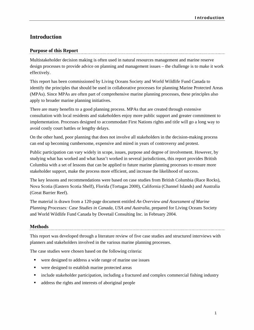
Introduction

Introduction

Purpose of this Report

Multistakeholder decision making is often used in natural resources management and marine reserve design processes to provide advice on planning and management issues – the challenge is to make it work effectively.

This report has been commissioned by Living Oceans Society and World Wildlife Fund Canada to identify the principles that should be used in collaborative processes for planning Marine Protected Areas (MPAs). Since MPAs are often part of comprehensive marine planning processes, these principles also apply to broader marine planning initiatives.

There are many benefits to a good planning process. MPAs that are created through extensive consultation with local residents and stakeholders enjoy more public support and greater commitment to implementation. Processes designed to accommodate First Nations rights and title will go a long way to avoid costly court battles or lengthy delays.

On the other hand, poor planning that does not involve all stakeholders in the decision-making process can end up becoming cumbersome, expensive and mired in years of controversy and protest.

Public participation can vary widely in scope, issues, purpose and degree of involvement. However, by studying what has worked and what hasn’t worked in several jurisdictions, this report provides British Columbia with a set of lessons that can be applied to future marine planning processes to ensure more stakeholder support, make the process more efficient, and increase the likelihood of success.

The key lessons and recommendations were based on case studies from British Columbia (Race Rocks), Nova Scotia (Eastern Scotia Shelf), Florida (Tortugas 2000), California (Channel Islands) and Australia (Great Barrier Reef).

The material is drawn from a 120-page document entitled An Overview and Assessment of Marine Planning Processes: Case Studies in Canada, USA and Australia, prepared for Living Oceans Society and World Wildlife Fund Canada by Dovetail Consulting Inc. in February 2004.

Methods

This report was developed through a literature review of five case studies and structured interviews with planners and stakeholders involved in the various marine planning processes.

The case studies were chosen based on the following criteria:

were designed to address a wide range of marine use issues

were designed to establish marine protected areas

include stakeholder participation, including a fractured and complex commercial fishing industry

address the rights and interests of aboriginal people

1

Introduction

Process Structure Framework

This report uses a process structure framework adapted from the principles suggested by several well-known authors of multistakeholder decision making in natural resources management and marine reserve design. This framework can be used to evaluate, design, and implement a collaboration initiative. It consists of:

A common purpose and definition of the problem and a commitment to collaborate

Inclusive and effective representation of interested parties

Effective process management

Effective process design

A structured and integrated decision-making framework

Equal access to information

Please see Appendix C for more details.

2

Recommendations for BC

Recommendations for BC

The following points summarize what conditions make a marine planning process successful, when a marine planning process is appropriate, and what conditions reduce the likelihood of a successful outcome, based on the common themes revealed in the five case studies.

What Makes a Process Successful

The following recommendations to ensure successful planning processes emerged from the five case studies:

Common Purpose Build trust. Some stakeholders will be concerned about the legitimacy of other stakeholder

involvement in a process. Process managers must allow time at the outset to build the trust and respect between stakeholders.

Educate and build awareness about a marine reserve/planning proposal long in advance of a process to avoid surprises, build knowledge, create interest, and increase the desire for ocean protection.

Take small steps. Begin with a small, but useful, non-controversial reserve.

Address fears of the floodgates opening by coordinating marine reserve proposals for places that make sense. Avoid enhancing the perception that reserves are ad hoc conservationist tools.

Ensure all members regard each other as legitimate participants. This takes time and also involves many points listed in the Representation section below.

Demonstrate government support through clear objectives, policies and financial and human resources. Top-down agency support and outside attention or profile lends significance to a process. If there are broader fisheries management policies and initiatives underway while a specific MPA process is deliberating, government should seek to provide clarity on the linkages between the two processes or policies.

Conduct pre-negotiation assessments. Before commencing a collaborative process, conduct a feasibility study to assess the value of collaboration. For example, assess the utility of a multistakeholder marine planning process, the level of support and understanding among users regarding marine reserves, and the need for a marine reserve from a socio-economic perspective, as well as a biological perspective. Include research on the utility of other means besides marine reserves to address the issues.

Ensure clear purpose through discussion and agreement.

Take an ecosystem approach. Coordination between and within government agencies will promote the legitimacy of the process and engender trust and participant commitment.

Ensure law and policy exists to mandate a marine planning process to develop and implement zoning. Legal mandates enhance fair, efficient, and consistent processes.

3

Recommendations for BC

Inclusive and Effective Representation Clarify who is to be involved in a process before starting the negotiation process so that

negotiations can begin with everyone working towards a solution together. Finding the right persons to be involved as representatives in a multistakeholder advisory group is one of the most difficult parts of the process and can take up to a year. Poor representation can mean delays in the process once it starts or once it has moved to the regulatory stage. Screen representatives for knowledge about the issues and make sure they won’t seek a pre-determined agenda.

Make sure participants can be effective representatives who are trusted and empowered by their constituency. This means spending time to manage complex or disorganized constituencies/sectors into caucuses or work groups.

Acknowledge the diversity of perspectives within a constituency and ensure they are adequately addressed in a marine planning process. One commercial fisherman or sport fisherman cannot speak for the whole industry. Ensuring the right balance of representatives even from within one constituency enhances participant trust and respect in a process.

Spend a substantial amount of time at the start of the process to become acquainted with all interested parties, both locally and beyond the region, and build relationships with them. Invite all interested parties into the process, but seek a balance of interests to avoid perception of power disparities. Engage average people from the various sectors and constituents, not only lobby groups or activists.

Consult First Nations communities as traditional users of marine resources. Invitations and follow up calls are necessary to obtain initial contact. Honorariums to cover transportation costs may be necessary. Identify respected community leaders to be involved in the process. Seek to develop tripartite cooperative management arrangements to address First Nations rights and interests in the marine area being planned. Because there are difficulties inherent with territorial overlap between tribes, First Nations must be allowed to decide how they wish to be represented in a process.

Build time for outreach. Design the process so that local representatives have the time and resources to plan and conduct outreach tasks. Develop a communication strategy that reaches out and informs widely (locally, regionally, provincially, nationally, internationally) and provide many opportunities for public input. Concerted outreach by process sponsors and grassroots activists targeting unorganized or alienated groups can help motivate people to attend public meetings and get involved in processes. Consider the creation of a Liaison Unit to engage with Indigenous coastal communities and identify and address Indigenous interests and concerns.

Involve community members and scientists as local expert stakeholders at the table so that they are part of a team for discussion, negotiation, and information gathering and dissemination.

Training or experience in consensus-based negotiations will enhance the effectiveness of representatives in a process.

Process Management Provide clear leadership, administration and facilitators. Ensure process managers are committed,

neutral, and skilled in process management and communication. Government sponsors should focus on facilitating, coordinating, and supporting processes. Staff should have the skills to teach and

4

Recommendations for BC

enable fishermen, local interested persons, and other constituent representatives to lead or chair meetings, and design processes as well as give presentations (Lane 2001). Sponsors should also supply the necessary resources for a process.

Use tripartite (or cooperative) arrangements to ensure successful planning and designation of MPAs. Involvement of First Nations must be government-to-government rather than as participants or stakeholders.

Employ impartial, expert facilitation to help structure and guide a process. Ensure that the facilitator is neutral but knowledgeable of the substantive issues.

Ensure active communications up and down the decision-making hierarchy. Keep advisory bodies as well as senior government and political decision-makers up to date with a community-based negotiation process.

Process Design Provide clear terms of reference for the overall process, even if they are drafts that require

consensus amongst participants, to provide direction and help move the process forward. Then let participants refine the terms of reference and seek constituent feedback to ensure the process will fit the community’s specific needs.

Ensure the scope and purpose of a process is made clear to all participants in a process before proceeding with substantive discussions. It may take several meetings, but taking the time to clarify mandate, roles, responsibilities, overall process framework and purpose will enhance understanding and trust, as well as prepare participants for what lies ahead.

Clarify early stakeholder expectations about outcomes of the process.

Be realistic about the amount of time required to develop a planning process. It takes time to identify issues and needs before seeking agreement on process or structure. Nevertheless, establish some milestones to guide people’s involvement. Ensure that a marine planning process works with the timelines of all stakeholder representatives involved in a process (e.g., check the fishing season so that fishermen can attend meetings). (Lane 2001)

Advisory Panels: Ensure that the expert panels that provide technical advice have clear terms of reference to avoid issues with the legitimacy of advice they provide.

Create a clear set of consensus-based decision rules and a fall-back dispute mechanism in case consensus cannot be reached. Resolve veto power by putting the onus on the person disagreeing to provide an alternative solution that will address their concerns and those of others. Do not place too much emphasis on the need for unanimity in a multistakeholder decision-making process. Something less than 100% will suffice for the process to still be considered consensus-based. The actual extent of agreement should be negotiated with the participants and not decided ahead of time by the process manager.

Take an ecosystem approach to process design as well as to reserve design. An ecosystem approach in reserve design increases the substantive issues that can be addressed in marine reserve collaborations (social, ecological, economic); an ecosystem approach to process design provides the means for involving all the agencies and groups whose jurisdictions crisscross the boundary area. A

5

Recommendations for BC

reserve therefore serves as a locus to coordinate and address interests and institutional responsibilities at all levels.

Avoid getting into mapping work before the ground rules and the upfront groundwork is completed.

Structured and Integrated Decision-Making Framework Use positive terminology to explain MPAs to commercial fishermen – “fisheries management

tools,” for example, not “no-take zones” (Lane 2001).

Use various techniques to involve participants. This will enhance meaningful and comprehensive involvement. Some people are uncomfortable with highly structured processes and may prefer time for open, frank, and less structured discussion (pers. comm. (15), 2001). Mixing small and large group discussions allows people to get to know one another at different levels, raises comfort levels, reduces fears and encourages the generation of ideas.

Develop a set of weighted selection criteria based on stakeholders’ values to help create better alternatives and assess how well those alternatives measure against the value-based criteria. Emphasize socio-economic considerations, not just the natural sciences of a reserve proposal. This is a foundation for process success, as well as the basis for the sustainability of the outcome.

Provide opportunities for the public to actively engage in workgroup discussions and contribute their local knowledge. During breakout group sessions, encourage participants to seek the input of constituents and others who attend meetings.

Be wary of perceptions of “behind-closed-door” solutions that may alienate participants.

Avoid independent review panels. Ensure that ecological, social and economic concerns and information are integrated equally into the process. Not setting up “expert science” panels avoids the dichotomies that are created between science and consumptive user groups.

Check in with participants during the process to identify how they perceive the meeting and whether any design parameters need to be changed.

Information Gathering and Dissemination Schedule a number of community meetings to ensure that all relevant communities and

representatives are invited to voice their opinions.

Do not underestimate the amount of science that is needed and the amount of time to acquire that knowledge. Information gathering is a good opportunity to build group relationships.

Invest resources and take the time to build user awareness about impacts to the marine environment. Disseminate information about MPAs, marine reserves, and issues of concern to increase understanding and awareness. Disseminate credible research and monitoring results from the region and abroad.

Use third-party researchers who are trusted by locals and who will follow protocols of confidentiality to obtain reliable socio-economic information.

Enlist locals to share their knowledge of the marine region. Recognize that some commercial fishermen, divers and salvors may not have academic training but they know as much about marine ecosystems as scientists, if not more. .

6

Recommendations for BC

Build fishermen’s trust and respect, as well as support, for the process and proposal - they may help with enforcement later on. Ensure fishermen understand the economic benefits available to them from protecting a particular site. If marine users are not informed about what the benefits (and the costs) are, they will be less supportive.

Learn about what matters to fishermen and coastal people. Do not rush into a process before learning to speak their language. Take the time to identify their values and why they may be for or against marine reserves.

Identify whether marine reserves are the best option. One result of joint fact-finding discovering whether it makes sense to protect an area or not as a marine reserve, or whether other marine planning means are more suitable.

Be sensitive to all users’ views and educate the public on both the pros and the cons of marine reserves for all user types so no single group feels it is being specifically targeted and impacted in the process.

Provide mapping technology at standardized scales as a means of assembling large amounts of information and allowing comparisons across a range of values. Provide support staff to assist the participants with GIS technology and mapping work.

Assemble all of the written documentation in one resource binder for each participant. Don’t overload the working group. Provide information far in advance of the start of the process and update as necessary.

7

Recommendations for BC

When a Process Should Proceed

A process should proceed if the following circumstances apply:

Common Purpose The agency has first considered whether an agreement-seeking approach is appropriate. For

example, the feasibility of a marine planning process and the level of support for such an initiative have been assessed before commencing or announcing such an initiative.

Key parties are committed to collaborate and are willing and able to participate.

The issue will not require compromise of basic values and principles. (First Nations will take the time to be involved in a marine planning process if it is developed on the basis of cooperative management of traditional resources).

The issue is “ripe” for discussion (e.g. a stalemate is unacceptable to several parties).

Government is likely to implement the agreement reached. Public participation includes the promise that the participants’ contribution will influence the decision.

Inclusive and Effective Representation Inclusive and effective representation is a key focus of the participation process; it seeks out and

facilitates the involvement of those potentially affected.

The process is coordinated with other government agency processes.

The process design includes reaching out to the general public to help ensure inclusive representation.

Stakeholder representatives demonstrate effective representation and maintain communication with their constituencies.

Stakeholder representatives have negotiation skills to build bridges between sectors.

Process Management There is support from relevant decision-making agencies.

A neutral third party facilitates discussions involving potentially high-conflict topics such as public lands, public waters, and natural resources.

Process Design Sufficient time is available to address the key issues.

Consensus is sought for small steps in the process (e.g., problem statement, goals/objectives, management intentions), not just in the outcome.

Participants help define how they participate.

Ground rules are mutually agreed upon by all participants.

There is a real possibility of success as defined by participants.

8

Recommendations for BC

Effective means of communication are used to reach constituents, including coordinating special gatherings, attending other meetings, chatting with people at local bars, connecting one-on-one, and going “down to the docks.”

Structured and Integrative Decision-Making Framework The process promotes an iterative approach to dealing with complex issues, develops decision

criteria, highlights trade-offs, identifies options, and balances social, economic and environmental concerns in the decision-making structure.

There is a chance to coordinate and integrate activities.

Interest groups feel that the framework provides a means of addressing growing user conflict.

Information Gathering and Dissemination The process promotes knowledge equality amongst all interested parties and participants to a

process, adding significantly to the general body of knowledge about marine reserves. This can involve having participants assist with information gathering, inviting expert speakers, sponsoring public sessions and special socio-economic and ecological forums, providing relevant and understandable documents, and producing other resources such as GIS mapping tools.

The process provides feedback to participants on how their input was used.

9

Recommendations for BC

When a Process Should Be Avoided

A process should be avoided in the following circumstances:

Lack of Common Purpose There is little or no incentive to solve a problem, meet a deadline, or engage adversaries because

participants have other means to work out their issues, such as lawsuits or political pressure.

The resource is too significant, sensitive, or otherwise unsuitable for negotiation.

The key issues require legislative or legal determinations outside the scope of the group.

The convening agency or authority lacks commitment to the process and to honouring process outcomes.

Poor and Ineffective Representation Participants lack the authority to make decisions on behalf of their constituency.

Participation requires an organization to compromise fundamental values.

Diverse representation is not available or key individual representatives cannot participate.

Ineffective Process Management Consensus rules are not enforced by the facilitator, creating a veto power.

Ineffective Process Design There is too high an emphasis on achieving a consensus agreement, putting too much pressure on

representatives, especially if they are not empowered to negotiate agreements.

Too little time is allowed for the collaborative process.

Poor Information Gathering and Integration Participants are unwilling or unable to accept new information and alter beliefs.

There isn’t fair access to independent expertise on technical issues

10

Recommendations for BC

11

Case Studies

Case Studies of Marine Planning Processes

United States: Tortugas 2000, Florida

This case study outlines the National Oceanographic and Atmospheric Administration’s (NOAA) community-based process for establishing a network of marine reserves in the Florida Keys National Marine Sanctuary. The process for Tortugas 2000 and the designation of the Tortugas Ecological Reserve involved eleven years of marine planning.

The Florida Keys National Marine Sanctuary was designated by Congress in November 1990 to address drastic declines in coral reef health and fish species and the risk of ships grounding on the shallow reefs (Ogden 1997). The 2,900 nm2 (9800 km2) Sanctuary encompasses the marine waters surrounding the Florida Keys archipelago. Today it contains a network of 24 no-take zones, including the Tortugas Ecological Reserve.

In 1991, the Sanctuary began a public process to develop the management plan and formed the multistakeholder Sanctuary Advisory Council to help ensure public input. In 1995, NOAA proposed a draft management plan (DOC 1995) for public review that originally included an ecological reserve, as well as a boundary for a 110-nmi2 no-take zone in the Tortugas area.

Despite the efforts of scientists and conservation organizations, local fishermen defeated the proposal for the Tortugas reserve (Ogden 1997). There was great misunderstanding and mistrust of the Sanctuary, lack of knowledge about marine reserves, and dissatisfaction with the public process the Sanctuary followed to develop the marine zoning system.

Subsequent drafts of the Management Plan proposed smaller and smaller sites, until finally, due to mounting public controversy, the Sanctuary eventually removed the Tortugas proposal from the plan completely (Ogden 1997).

However, Sanctuary officials did not give up on Tortugas. Local and international evidence was being published on the positive effects marine reserves were having on biodiversity and fisheries. Together with the National Park Service, they launched a collaborative process – Tortugas 2000 – that brought together a group of stakeholder representatives to recommend more acceptable boundaries for the Tortugas area that would satisfy conservation concerns without ignoring socio-economic needs (DOC 2000).

Phase I (April 1998 to June 1999) involved the design of the reserve, including a series of public meetings to determine the range of issues to be considered. A Work Group of agency officials, representatives from user groups (such as commercial fishermen and the dive industry), environmental organizations, and other concerned citizens was then formed and charged with recommending a set of alternative boundaries for comment.

The Work Group agreed on an ecological reserve in two portions. The 91nm2 Tortugas North, designed to protect coral reef resources, allows diving but no consumptive uses. The 60nm2 Tortugas South, designed to protect a coral reef system, commercial fish species, and associated habitat, does not allow diving or consumptive uses.

12

Case Studies

Successes There was a high level of participant support for the process, due partly to the perception that government had learned its lessons from the original, flawed marine zoning process and partly to a new, bottom-up approach. By 1998, the public could also see benefits of no-take zones locally and internationally. The Sanctuary Superintendent’s long-term commitment, leadership, and local credibility were very important, as was a core staff that was critical in moving the process forward.

The Work Group made sure that missing interests were invited to the table, demonstrating commitment to an inclusive process. The process for selecting stakeholder representatives was considered clear, fair and comprehensive. Spending time on groundwork helped to build relationships and develop trust.

Integrating the scientists and the local traditional knowledge experts into the Work Group also built trust, and the wealth of knowledge that fishermen possessed was a great benefit. Use of GIS mapping to display ecological and socio-economic information was helpful in negotiating the location, size and allowable uses in the Tortugas Ecological Reserve. Disseminating research and monitoring results was critical in shifting pubic opinion. Likewise, constituent outreach was a key feature of ensuring effective representation.

Consensus decision making ensured that all concerns were addressed in the process, moving people away from extremes or positional bargaining (pers. com. (14) 2001) and achieving compromise. Considering a balance of the social and economic issues along with the ecological issues was fundamental to the success of the process. Finally, the process was designed so that common criteria were agreed on before the contentious discussions about maps, reserve locations or percentages occurred.

Challenges The greatest opposition to the process came from national recreational fishing groups, who opposed the principle of closing any waters to recreational fishing. In addition, lack of clarity with the marine reserve objectives before the start of the process led to some confusion and mistrust, especially from the sport fishermen.

Finding the right Work Group participants was one of the most difficult parts of the process. Some participants couldn’t openly represent and commit their constituencies at the table, and failing to secure a sport fishing representation early on was a problem, given the media coverage generated by sport fishing interests.

13

Case Studies

United States: Channel Islands, California

This case study outlines the National Oceanographic and Atmospheric Administration’s (NOAA) community-based process for establishing a network of marine reserves in California’s Channel Islands National Marine Sanctuary. The Sanctuary was designated in September 1980, and consists of 1,252 square nautical miles of open ocean and near-shore habitat approximately 25 miles off the coast of Santa Barbara.

In 1998 local citizens, fishermen and the Channel Islands National Park approached the California Fish and Game Commission with a proposal for a network of marine reserves within the Sanctuary. The result was a joint process to discuss MPAs in the Channel Islands area, including the appointment of a 17-member Marine Reserves Work Group (MRWG).

The MRWG included members of the Sanctuary Advisory Council (an advisory group of constituents), government agencies, and representatives of the public, commercial fishing, recreational fishing, sport and commercial diving interests, and non-consumptive interests. A Science Advisory Panel and a Socioeconomic Panel provided technical expertise, and input was gathered from public forums and comments.

While the MRWG did not reach consensus on reserve boundaries, it agreed on a problem statement, issues of concern, goals and objectives and implementation recommendations, producing the foundation for what has become the state-level network of MPAs and marine reserves, and what will soon become the federal waters portion of the network. During the nearly two-year process, the group developed over thirty potential marine reserve network maps which they whittled down to two, but ultimately they could not achieve consensus on the use of limited take, size, and the location of the reserves.

A series of bodies evaluated the MRWG’s efforts: the Channel Islands Sanctuary Advisory Council, the Sanctuary Manager and staff, the Department of Fish and Game, and finally, the Fish and Game Commission. The MRWG’s package of agreements and information gathered during process formed the basis of the Commission’s final recommendation.

In October 2002, the Commission approved NOAA’s and the Department’s preferred alternative for a network of twelve marine reserves and various types of MPAs, ranging from limited to full protection, covering 142 nmi2 of the Sanctuary.

Successes: Reaching out to constituencies was critical to the process and to ongoing relationships. As a result of the MRWG, more fishing communities became interested and involved in the process of marine planning – not only in the MRWG but in the wider state process. The process was designed to directly involve representatives in meeting design, and consensus decision making encouraged a broad alliance of interests.

Gathering and disseminating information – including local knowledge – involved a great deal of time, money, and research, but was invaluable to the Sanctuary, the MRWG members and the general public.

14

Case Studies

Challenges Poor choice of terminology and the lack of pre-negotiation assessment made it more difficult to build support and establish a common purpose. For example, terms like “no-take zones” and “over-fishing” often disengaged fishermen and other marine users.

There were several problems with representation. When one conservation representative withdrew, the open seat was not filled, which affected the perception of balance and the legitimacy of the process. Some representatives in the MRWG did not reflect the views of constituents, while others lacked the authority to make decisions for their constituents (Davis 2001). Some, like oil and gas and yachting interests, were missing entirely.

Some MRWG members felt that too much emphasis was placed on unanimity and that something less than 100% would have sufficed. Drawing lines on maps and discussing percentages created some of the greatest conflict in the process. In addition, the group was unsure how to address a reserve network in the Channel Islands with little knowledge about fisheries management outside of reserves.

Finally, there was too much pressure on the MRWG to deliver a recommendation within too short a time to prevent the state government from stepping in and making decisions. More time was needed to build relationships between divergent interests.

Australia: Great Barrier Reef, Queensland

This case study outlines the Great Barrier Reef Marine Park Authority’s process for involving Aboriginal and Torres Strait Islander peoples in the planning and management of Queensland’s Great Barrier Reef Marine Park and World Heritage Area. Two sets of property rights and responsibilities overlap in this region: Indigenous Australians’ native title rights, and national/state governance of the area as a multiple-use MPA (Innes and Ross 2001).

From the Authority’s perspective, one of the hardest issues to address has been the culturally appropriate and ecologically sustainable management of traditional hunting (GBRMPA 2003e). It therefore developed an Indigenous Policy and Liaison Unit to help address the legal issues and concerns of local Indigenous peoples (GBRMPA 2003a).

Under the Representative Areas Program, the Authority rezoned the Marine Park based on 70 distinct bioregions with community input. During the initial public consultation, the Liaison Unit informed and sought input from Aboriginal and Torres Strait Islander peoples, reference groups, land councils, community groups and corporations, leading to the development of a draft zoning plan for the Great Barrier Reef.

Next, 18 regional workshops on the reef-wide Traditional Hunting Framework were held with Indigenous communities (GBRMPA 2003f). Then the Draft Zoning Plan was released for public comment, one of the largest examples of public involvement in any environmental issue in Australia’s history.

As a result of the consultations, a new provision for Traditional Use of Marine Resource Agreements (TUMRAs) was introduced. TUMRAs are formal agreements with Aboriginal and Torres Strait Islander Traditional Owner groups who assert rights and interests in the Marine Park (GBRMPA 2003a). They

15

Case Studies

provide a framework for addressing a range of Marine Park issues that Traditional Owner groups will help to manage.

Under the proposed management arrangements in the draft Zoning Plan 2003, traditional fishing and collection will not require written permission from the Authority in zones that allow fishing and collecting. Traditional Owners will continue to have access to all zones in the Marine Park for traditional activities that don’t involve taking animals, plants or marine products. In more highly protected zones, traditional uses will be managed under TUMRAs.

The public and community consultations on the new Zoning Plan have resulted in 33 percent protection in highly protective no-take areas (GBRMPA 2003a).

Successes Indigenous representation is the greatest success of the rezoning process. For the first time, Indigenous communities became more involved, visible, and represented at a reef-wide level. Aboriginal and Torres Strait Islander peoples are taking a proactive approach to addressing traditional use of marine resources, leading to the development of cooperative management arrangements (TUMRAs) in the Marine Park.

The Authority has played a key role in ensuring Indigenous involvement in Park management. Because of the wide and often remote distribution of the region’s Indigenous population, an effective cross-cultural communication strategy has been critical.

Challenges The main challenge arises when Traditional Owners oppose certain activities in a particular area of the sea country. The Liaison Unit can now respond with planning tools such as TUMRAs to support Traditional Owners’ involvement in issue identification, cultural mapping, and cooperative management of their traditional area.

Canada: Race Rocks, British Columbia

This case study outlines First Nations involvement in Fisheries and Oceans Canada’s / Race Rocks Marine Protected Area planning process, particularly in the Race Rocks Advisory Board. (pronounced shwai’yen) is the name given to the area by the Coast Salish Nations and means “swift waters.”

Under the Oceans Act 1997, Fisheries and Oceans Canada (DFO) is responsible for coordinating marine protected area initiatives between agencies and between federal and provincial jurisdictions. It is also mandated to designate its own national system of MPAs1 through collaboration and cooperation with other governments, agencies, affected First Nations organizations, and coastal communities. These should ideally be situated within integrated management plans based on an ecosystem approach. Special consideration is given to traditional activities in marine areas, and all decisions should be consistent with First Nations land claims agreements (DFO 1998).

1 In this case study, the term “MPAs” refers to DFO’s system of marine zoning designation under the Oceans Act. In the rest of the report, the term “MPAs” refers to the meaning defined in the glossary.

16

Case Studies

In 1980, the province designated Race Rocks as an ecological reserve, providing protection for the natural and cultural heritage values of nine islets and the ocean bottom. Eight years later, /Race Rocks Ecological Reserve was declared an Area of Interest under the Oceans Act and the Federal–Provincial MPA Strategy and was selected as an MPA pilot. The next step was for DFO to assess whether it met the designation criteria and then identify and assess its ecological, technical and socio-economic merits.

To help in the process, a multistakeholder Race Rocks Advisory Board was established in 1999 that included government, First Nations and local stakeholder representatives. The Advisory Board reached consensus on recommendations to support an MPA designation, including provisions for the creation of a no-take zone and the establishment of a co-management regime involving First Nations, British Columbia and Canada (DFO 2000a).

The Minister of Fisheries and Oceans subsequently announced as Canada's first MPA under the Oceans Act in September 2000. However, to date, the MPA was has not been formally designated due to complications in the regulatory process in Ottawa.

Successes Thanks to creative problem solving, the Race Rocks Advisory Board was able to negotiate a no-take zone within the boundaries of the existing ecological reserve, gain First Nations’ support for the creation of a Marine Protected Area, adopt a First Nations name for the area, and recommend co-management by local First Nations, B.C. Parks and DFO.

Challenges Despite the Advisory Board’s success in developing recommendations, once these recommendations were submitted, they were misrepresented in the proposal and in the federal government’s regulatory approval process. Both the misrepresentation and the subsequent protest involved groups that were not part of the Advisory Board (LeRoy 2002).

DFO’s proposal document excluded the possibility of First Nations being part of a tripartite cooperative management arrangement, which was agreed to by the Advisory Board.

The local First Nations Chiefs T’souke, Songhees and Beecher Bay opposed the proposed MPA, citing Delgamuk, infringement of rights, and lack of consultation, halting the final designation (LeRoy 2002). DFO learned that First Nations representatives on the Advisory Board did not have the support from local First Nations to negotiate on their behalf.

DFO has since consulted with the Chiefs and acknowledged that it did not engage with the First Nations effectively. The Chiefs responded with a letter of support for the MPA on the condition of true co-operation and acknowledgement of Douglas Treaty Rights.

17

Case Studies

Canada: Eastern Scotia Shelf, Nova Scotia

This case study outlines Fisheries and Oceans Canada’s Eastern Scotian Shelf Integrated Management (ESSIM) process and the Gully Marine Protected Area process. As noted in the previous case study, Fisheries and Oceans Canada (DFO) is responsible for developing a national system of MPAs based on an integrated management approach.

The Eastern Scotian Shelf Integrated Management (ESSIM) Initiative is an ongoing collaborative offshore planning and management process for the Eastern Scotian Shelf Large Ocean Management Area being led by DFO. It was announced in December 1998 following the Sable Gully Conservation Strategy’s recommendation to apply integrated management approaches to the offshore area surrounding the Sable Gully Area of Interest.

Key interests on the Shelf – an area of high biological diversity and productivity – include fisheries, offshore oil and gas, shipping, maritime defence operations, submarine cables, science, research and development, recreation and tourism, potential offshore minerals development, and marine conservation (DFO Maritimes Region 2001).

To date, an array of sectoral meetings have been held, background reports written, and two workshops conducted. An “ESSIM Forum” has been proposed along with a supporting administrative ESSIM Secretariat, and a Federal-Provincial ESSIM Work Group has been formed, along with other multistakeholder work groups.

Gully MPA The Gully is a deep canyon ecosystem on the edge of the Scotian Shelf, near Sable Island, that has been the focus of conservation efforts since the early 1990s (Canada Gazette 2003).

A Work Group and an Advisory Committee have been formed to develop the MPA and management plan. Based on the Work Group deliberations, DFO developed a document in 2002 outlining the proposed MPA and management zone boundaries, and described the scope and intent of the regulations being developed. It was distributed to offshore industries, academia, government agencies, First Nations, environmental interest groups and other non-government organizations. DFO also gave presentations and held separate meetings with key interests during 2002–2003.

Although the Gully MPA is distinct from the broader ESSIM Initiative in terms of scale and scope, the two planning processes are nested together and involve many of the same interests and management issues. The ESSIM process will continue to support Gully MPA planning, as well as the identification and development of an MPA system plan for the Scotian Shelf (Canada Gazette 2003).

Successes To date, the intent, objectives and processes proposed for the ESSIM Initiative have been received favourably by participants (DFO Maritimes Region 2001). Through ESSIM processes, DFO has demonstrated its willingness to collaborate, and although the process is taking longer than expected, there is a general belief that an integrated management plan will improve the situation on the Shelf.

18

Case Studies

Because DFO is a process sponsor instead of a process facilitator – meetings are co-chaired and workshops led by a neutral facilitator – it can focus on the discussion issues.

By integrating the Gully MPA process in the ESSIM Initiative, multiple uses and impacts beyond the MPA can be managed to meet the Gully’s ecosystem protection requirements. The iterative cycles and feedback loops among the five stages allow the integrated management plan to be adapted to address the dynamic nature of the ecosystem and/or human uses of the ecosystem.2

Challenges Some participants do not acknowledge the legitimacy of other stakeholders, and fishing interests are not always willing to discuss management in a multisectoral context. It will take more time to build trust and respect. As well, DFO suffers from some lack of public trust because it is seen as “the violator” of fisheries management on the East Coast.

Participants want DFO to take a greater leadership role and begin implementing some of the planning to date. There continues to be the perception that DFO is not well coordinated internally, and DFO staff does not have adequate resources to perform its Secretariat functions appropriately.

There are many different perspectives and interests involved within a constituency, making it difficult and undesirable for people to identify themselves as spokespersons for their constituency. It is also difficult to identify and engage all interests. In addition, some constituents can’t afford to attend meetings regularly.

2 Source: http://www.mar.dfo-mpo.gc.ca/oceans/e/essim/essim-reports-planningprocess-e.html.

19

Appendices

Appendix A: Glossary

Collaboration: Collaborative processes include a mix of individuals representing often conflicting interests and views who come together either because of a shared vision (proactively) or because of conflict (reactively) to meet the goals of all the group members. Also called multistakeholder decision making and natural resource decision making.

Indigenous: In Australia the term Indigenous is used to refer to both Aboriginal and Torres Strait Islander peoples. This document will often use the term Indigenous to refer to both First Nations in Canada and Aboriginal and Torres Strait Islanders in Australia.

Integrated oceans and coastal management (IM): A comprehensive and coordinated approach to decision making, based on a balanced consideration of the full range of interests and associated ecosystem, social and economic objectives for a management area.

Marine Protected Areas: According to the World Conservation Union (IUCN), any area of intertidal or subtidal terrain, together with its overlying water and associated flora, fauna, historical or cultural features, which has been reserved by law, or other effective means, to protect part of the entire enclosed environment.

Marine reserves: Areas in the ocean where no take of living or non-living marine resources is allowed. Also called no-take areas or no-take zones.

Stakeholders: Anyone who is able to affect or be affected by an outcome of any negotiation, who is responsible for implementing its decision(s), and who has an interest in the issues. Also called interested parties.

20

Appendices

Appendix B: Literature Cited

Canada Gazette. 2003. Gully Marine Protected Regulations – Regulatory Impact Analysis Statement. C.Gaz. 2003, I. 3382. (Oceans Act). On line: http://canadagazette.gc.ca/partI/2003/20031206/ html/regle1-e.html

Davis, Craig. 2001. Channel Islands National Park Service. Proceedings of the MPA Powertools Conference - Building the Marine Protected Area Movement from the Grassroots Up. (unpublished). White Rock BC, October 19-21, 2001. Living Oceans Society.

Department of Commerce (DOC). 1995. Draft environmental impact statement / Draft management plan for the Florida Keys National Marine Sanctuary. Silver Spring, MD: NOAA.

DFO Maritimes Region. 2001. The Eastern Scotian Shelf Integrated Management (ESSIM) Initiative - Development of a Collaborative Management and Planning Process - A Discussion Paper prepared for the Federal-Provincial ESSIM Work group. November 2001. Oceans and Coastal Management Division, Oceans and Environment Branch, Fisheries and Oceans Canada, Maritimes Region. On line at: http://www.mar.dfo-mpo.gc.ca/oceans/e/essim/essim-reports-planningprocess-e.html

DFO. 1998. Marine protected areas program. Fisheries and Oceans Canada, Communications Directorate, Ottawa, ON

DFO. 2000a. Draft Race Rocks Marine Protected Area Feasibility Report and Recommendations. May 2000. On line at: http://www.racerocks.com/racerock/admin/rrab/draftrrfeasibility.htm #Anchor-Acknowledgements-11481

GBRMPA. 2003a. Frequently Asked Questions. On line: http://www.reefed.edu.au/rap/pdf/FAQs_3Dec2003.pdf .

GBRMPA. 2003e. Sea Country Newsletter. No. 10: June 2003

GBRMPA. 2003f. Annual Report 2002-2003. On line: http://www.gbrmpa.gov.au/corp_site/ info_services/publications/annual_reports/AR2002-2003.pdf

Innes J. and H. Ross. 2001. Co-managed research as a strategy for informing the development of indigenous and government management partnerships over the Great Barrier Reef. Presented at: Regional Conference of the International Association for the study of Common Property, Brisbane, Australia, 2-4 September 2001. Staff Paper 2001-12. Great Barrier Reef Marine Park Authority, Townsville, Qld.

Lane, David. 2001. T Buck Suzuki Environmental Foundation. Proceedings of the MPA Powertools Conference - Building the Marine Protected Area Movement from the Grassroots Up. (unpublished). White Rock BC, October 19-21, 2001. Living Oceans Society.

LeRoy, S. 2002. Public Process and the Creation of a Marine Protected Area at Race Rocks, British Columbia. Masters Thesis. School of Community and Regional Planning, University of British Columbia, Vancouver, B.C. On line at: http://www3.telus.net/LeRoy/Portfolio/racerocks.pdf

Ogden, J. 1997. Marine managers look upstream for connections. Science. 278(5342): 1414-1415.

21

Appendices

Appendix C: Process Structure Framework

The following table describes the process structure framework used in this report, adapted from the principles suggested by several well-known authors of multistakeholder decision making in natural resources management and marine reserve design.3 This framework can be used to evaluate, design, and implement a collaboration initiative.

a) Participants: Participants acknowledge the need for a consensus-building process and are committed to it, acknowledge the legitimacy of other stakeholders, and agree on a common definition of the issues at stake.

1. Common Purpose and Definition of Problem & Commitment to Collaborate

b) Government: Government demonstrates leadership, commitment and integrity by establishing clear objectives, providing timely and clear policies, allocating financial and human resources, and acting on consensus recommendations; ensures coordination with existing policies and decision-making processes; and supports participation by its agencies and their representatives. Government assesses the appropriateness of negotiation prior to the start of process.

a) Inclusive representation: Everyone who is able to affect or be affected by the outcome of any negotiation, who is responsible for implementing decisions, and who has significant interest in the issues should be involved in the negotiations. The wider public is kept informed through outreach methods. The process involves local, government and First Nations interests as needed. Inclusion is a process of continual adaptation with differing levels/roles for representatives. Complex constituencies are managed into caucuses. The set and number of stakeholders reflect the complexity of the problem.

2. Inclusive and Effective Representation of Interested Parties

b) Effective representation: All participants are committed – they attend regularly, participate in good faith, are knowledgeable, communicate openly and share ideas. Representatives are trusted by their constituents and empowered to represent them and make decisions on their behalf; they maintain communication with and inform their constituencies. Government representatives can speak for their organization, are available for consultation, are skilled in communication and public processes, listen to participants, are technically knowledgeable, understand planning, work well with people, and share power with public representatives.

3. Effective Process Management

Process managers include convenors, co-ordinators, administrators, and facilitators. In addition to having the attributes described under Effective Representation, process managers are committed, neutral, skilled in process management and communication, knowledgeable about issues; and available for consultation with participants. Stakeholders must believe process managers have legitimate authority. Leadership and constructive management throughout the process are critical to success. High interdependence in a group requires powerful convenors. High-conflict situations suggest the need for professional facilitators.

3 The main authors are: Dukes and Firehock 2001; Duffy, Hallgren, Parker, Penrose, and Roseland 1998; Gray 1989; Cormick, Dale, Edmond, Sigurdson and Stuart 1996; Roberts and Hawkins 2000.

22

Appendices

a) Clear terms of reference: The mandate, roles, responsibilities, and authority are clear to all participants. Clear terms of reference also involve a clear purpose of process; clarity of stakeholder expectations about outcomes; clear organization, roles and authority of subgroups; clear ground rules; and realistic timeframes. The process is flexible and adapts to changing circumstances; a fall-back dispute mechanism exists if consensus is not reached. The geographic scale is appropriate. Meeting logistics are clear, and a media policy is agreed upon.

b) Participatory design: Participants are involved in tailoring their mandate, process, issues, and agenda. The agenda is designed to accommodate all interests and includes ground rules for operating together. Mechanisms are in place to allow participants to provide feedback and to facilitate change to the process design. There are trade-offs between the number of stakeholders and the ease of managing a process.

4. Effective Process Design

Effective process design requires clear terms of reference to guide the process, participant involvement in the process design, and a comprehensive set of procedural ground rules.

c) Ground rules: The rules of procedure must be clear to establish boundaries for participant behaviour as well as the procedure and substance of the discussions (e.g., organization, conduct and logistics of meetings). Ground rules cover participant interactions, issues up for discussion, parties at the table, information sharing, facilitation, dispute settlement process, decision rules, and consensus rules. Without agreement on these matters there can be no process. The process design is effective only if stakeholders adhere to procedural agreements.

a) Structured decision-making framework: The decision-making framework is rigorous, uses an iterative approach to deal with complex issues, and highlights trade-offs. It manages the complexity of substantive issues through explicit decision criteria used to explore options, clarify decisions, and monitor and evaluate decisions. Inventing options of differing strength increases the number of potential solutions.

b) Creative approaches to problem solving: Creative approaches to promote teamwork and effective problem solving are utilized; e.g., small group sessions, plenary or roundtable discussions, forums, speakers, and mapping tools. Sub-groups/sub-committees or a neutral third party can help present and scrutinize multiple options. Time is built into the process to understand differences. Trust is built by working to achieve the principles in this framework, by ensuring interest-based negotiations, by holding specific workshops to address barriers between groups and develop skills, and by exploring options and making trade-offs together.

5. Structured and Integrative Decision-Making Framework

Providing structure to the decision process creates opportunities for meaningful involvement of all participants in deciding the substantive issues through the achievement of each of the following sub-sections, in development, evaluation and selection of decision alternatives.

c) Comprehensive and integrative framework: The process promotes decisions that consider balancing social, economic and environmental impacts, issues, and concerns.

a) Equal access to information: “Knowledge equality” improves the balance of power and ensures all participants, including government agency staff, can participate meaningfully. This means providing resources to assemble information and providing access to, and dissemination of, information and expert knowledge. Expertise includes local and traditional knowledge. Information is the best available, credible, understandable, timely, not rushed or late. Experts are made available to explain and interpret information and assumptions.

6. Equal Access to Information

b) Joint information search: Joint fact finding allows all participants to mutually gather, examine and share information relevant to decisions. Together, participants assign tasks or teams or invite panels of experts to synthesize complex and controversial data (social, economic, scientific, layperson/traditional/local knowledge) to help stakeholders understand. Third parties can be contracted to research information that is missing or difficult to obtain.

23