bining com
TRANSCRIPT

Combining
Garbage Collection
and
Region Inference
in
The ML Kit
Niels Hallenberg ([email protected])
Department of Computer Science
University of Copenhagen
Master's Thesis
June 25, 1999

Preface
The ML Kit is a Standard ML compiler where memory management is based
on region inference. Region inference inserts, at compile time, allocation
and deallocation directives into the target program such that no dynamic
memory management is necessary (i.e., garbage collection). However, it is
not always possible to insert allocation and deallocation directives such that
all dead memory is reclaimed for reuse. It is therefore interesting to see if it
is possible to combine region inference with garbage collection. The bene�t
should be that most of the allocated memory is recycled e�ciently by region
inference and the garbage collector concentrates on the memory not recycled
by region inference. The goal is a system that recycles memory eagerly (i.e.,
uses less memory) and e�ciently (i.e., uses less time on recycling memory).
We present a new backend for the ML Kit which has been designed with
a garbage collector in mind. The backend in the ML Kit, as released in
version 3, mainly consists of one large module compiling the intermediate
lambda language into three address code. We have organized the new back-
end di�erently and split it into many smaller modules. Each module is then
simpler to comprehend and debug.
We also present a garbage collector that works with regions. Region
inference complicates the task of garbage collection in many ways. For
instance, the heap is split in many smaller heaps called region pages and
some of the heap allocated objects are actually allocated on the machine
stack.
Acknowledgements
I would like to thank my advisor Mads Tofte for his inspiration, excellent
supervision and ideas without which this project would not have been pos-
sible; many aspects of the compiler is the result of his guidance. I will also
thank Martin Elsman for his interest in this project and all the discussions
we have had about the ML Kit and this project.
Also thanks to the other members of the ML Kit group, that is, Peter
Bertelsen, Lars Birkedal, Tommy H�jfeld Olesen and Peter Sestoft. It is
always a lot of fun to work in the ML Kit group.
1

Contents
I Overview 7
1 From Manual to Automatic Memory Management 8
1.1 Overview of The Compiler . . . . . . . . . . . . . . . . . . . . 12
1.2 Reading Directions . . . . . . . . . . . . . . . . . . . . . . . . 13
1.3 What Has Been Implemented . . . . . . . . . . . . . . . . . . 14
1.4 Performance . . . . . . . . . . . . . . . . . . . . . . . . . . . . 15
1.5 Notation . . . . . . . . . . . . . . . . . . . . . . . . . . . . . . 15
II The Backend 17
2 RegExp 18
2.1 The Region Inference Allocation Strategy . . . . . . . . . . . 18
2.2 Region Inference . . . . . . . . . . . . . . . . . . . . . . . . . 20
2.2.1 Dynamic Semantics for RegExp . . . . . . . . . . . . . 21
2.2.2 Example Program . . . . . . . . . . . . . . . . . . . . 30
2.3 Multiplicity Inference . . . . . . . . . . . . . . . . . . . . . . . 31
2.3.1 Example Program . . . . . . . . . . . . . . . . . . . . 32
2.4 K-normalization . . . . . . . . . . . . . . . . . . . . . . . . . 33
2.5 Storage Mode Analysis . . . . . . . . . . . . . . . . . . . . . . 33
2.5.1 Example Program . . . . . . . . . . . . . . . . . . . . 35
2.6 Physical Size Inference and Drop Regions . . . . . . . . . . . 36
2.7 Application Conversion . . . . . . . . . . . . . . . . . . . . . 37
2.7.1 Example Program . . . . . . . . . . . . . . . . . . . . 37
2.7.2 Example Program - Tail Recursive . . . . . . . . . . . 38
3 Closure Conversion 40
3.1 From Imperative Languages to Functional Languages . . . . . 40
3.1.1 Functions in Pascal . . . . . . . . . . . . . . . . . . . . 41
3.1.2 Functions in C . . . . . . . . . . . . . . . . . . . . . . 43
3.1.3 Functions in SML . . . . . . . . . . . . . . . . . . . . 45
3.1.4 Uniform Representation of Functions . . . . . . . . . . 46
3.1.5 Closure Representation . . . . . . . . . . . . . . . . . 47
2

CONTENTS 3
3.1.6 A Closure is Not Always Needed . . . . . . . . . . . . 48
3.1.7 Region polymorphic functions . . . . . . . . . . . . . . 50
3.1.8 Closure Explication . . . . . . . . . . . . . . . . . . . 52
3.2 Calculating the Need For Closures . . . . . . . . . . . . . . . 52
3.2.1 Variables and Constants . . . . . . . . . . . . . . . . . 53
3.2.2 Boxed Expressions . . . . . . . . . . . . . . . . . . . . 54
3.2.3 Expressions . . . . . . . . . . . . . . . . . . . . . . . . 54
3.3 ClosExp . . . . . . . . . . . . . . . . . . . . . . . . . . . . . . 57
3.3.1 Call convention . . . . . . . . . . . . . . . . . . . . . . 57
3.3.2 Functions . . . . . . . . . . . . . . . . . . . . . . . . . 59
3.3.3 Storage Modes . . . . . . . . . . . . . . . . . . . . . . 64
3.3.4 Grammar for ClosExp . . . . . . . . . . . . . . . . . . 64
3.3.5 Dynamic Semantics for ClosExp . . . . . . . . . . . . 65
3.4 Closure conversion . . . . . . . . . . . . . . . . . . . . . . . . 72
3.4.1 Preserve K-normal form . . . . . . . . . . . . . . . . . 72
3.4.2 Call Conventions . . . . . . . . . . . . . . . . . . . . . 73
3.4.3 Algorithm C . . . . . . . . . . . . . . . . . . . . . . . . 74
3.5 Re�nements of the Representation of Functions . . . . . . . . 83
4 Linearization 86
4.1 Scope of Regions and Variables . . . . . . . . . . . . . . . . . 86
4.2 Return Convention . . . . . . . . . . . . . . . . . . . . . . . . 88
4.3 LineStmt . . . . . . . . . . . . . . . . . . . . . . . . . . . . . 89
4.4 Example . . . . . . . . . . . . . . . . . . . . . . . . . . . . . . 90
4.5 Algorithm L . . . . . . . . . . . . . . . . . . . . . . . . . . . . 90
4.5.1 Top level declarations . . . . . . . . . . . . . . . . . . 92
4.5.2 Simple Expressions . . . . . . . . . . . . . . . . . . . . 92
4.5.3 Expressions . . . . . . . . . . . . . . . . . . . . . . . . 92
5 Register Allocation 95
5.1 Revised Grammar . . . . . . . . . . . . . . . . . . . . . . . . 97
5.1.1 Store Type . . . . . . . . . . . . . . . . . . . . . . . . 98
5.1.2 Call Conventions . . . . . . . . . . . . . . . . . . . . . 100
5.1.3 Resolving Call Conventions . . . . . . . . . . . . . . . 101
5.1.4 Rewriting LineStmt . . . . . . . . . . . . . . . . . . . 102
5.2 Dummy Register Allocator . . . . . . . . . . . . . . . . . . . 107
5.3 Liveness Analysis . . . . . . . . . . . . . . . . . . . . . . . . . 107
5.3.1 Def and Use Sets for LineStmt . . . . . . . . . . . . . 109
5.4 Interference Graph . . . . . . . . . . . . . . . . . . . . . . . . 109
5.4.1 Unnecessary Copy Related Interferences . . . . . . . . 110
5.4.2 Move Related Nodes . . . . . . . . . . . . . . . . . . . 110
5.4.3 Building IG . . . . . . . . . . . . . . . . . . . . . . . . 110
5.5 Spilling . . . . . . . . . . . . . . . . . . . . . . . . . . . . . . 112
5.5.1 Statements Are Not Like Three Address Instructions . 113

CONTENTS 4
5.6 Graph Coloring With Coalescing . . . . . . . . . . . . . . . . 114
5.6.1 Conservative Coalescing . . . . . . . . . . . . . . . . . 115
5.6.2 Spill Priority . . . . . . . . . . . . . . . . . . . . . . . 115
5.6.3 Implementation . . . . . . . . . . . . . . . . . . . . . . 115
5.7 Caller and Callee Save Registers . . . . . . . . . . . . . . . . 115
5.8 Example . . . . . . . . . . . . . . . . . . . . . . . . . . . . . . 117
6 Fetch And Flush 123
6.1 Revised Grammar . . . . . . . . . . . . . . . . . . . . . . . . 124
6.2 Set Of Variables To Flush . . . . . . . . . . . . . . . . . . . . 126
6.2.1 Top Level Functions . . . . . . . . . . . . . . . . . . . 126
6.2.2 Statements . . . . . . . . . . . . . . . . . . . . . . . . 126
6.3 Insert Flushes and scope reg . . . . . . . . . . . . . . . . . . 128
6.3.1 Top Level Functions . . . . . . . . . . . . . . . . . . . 128
6.3.2 Statements . . . . . . . . . . . . . . . . . . . . . . . . 129
6.4 Insert Fetches . . . . . . . . . . . . . . . . . . . . . . . . . . . 131
6.4.1 Top Level Functions . . . . . . . . . . . . . . . . . . . 131
6.4.2 Statements . . . . . . . . . . . . . . . . . . . . . . . . 131
6.5 Example . . . . . . . . . . . . . . . . . . . . . . . . . . . . . . 133
7 Calculate O�sets 136
7.1 Revised Storage Type . . . . . . . . . . . . . . . . . . . . . . 136
7.2 Algorithm CO . . . . . . . . . . . . . . . . . . . . . . . . . . . 137
7.2.1 Top Level Functions . . . . . . . . . . . . . . . . . . . 137
7.2.2 Statements . . . . . . . . . . . . . . . . . . . . . . . . 138
7.3 Example . . . . . . . . . . . . . . . . . . . . . . . . . . . . . . 138
8 Substitution and Simplify 141
8.1 Revised Grammar . . . . . . . . . . . . . . . . . . . . . . . . 142
8.2 Algorithm SS . . . . . . . . . . . . . . . . . . . . . . . . . . . 142
8.2.1 Top Level Functions . . . . . . . . . . . . . . . . . . . 142
8.2.2 Statements . . . . . . . . . . . . . . . . . . . . . . . . 144
8.3 Example . . . . . . . . . . . . . . . . . . . . . . . . . . . . . . 146
9 Code generation 148
9.1 Kit Abstract Machine . . . . . . . . . . . . . . . . . . . . . . 148
9.1.1 Grammar for KAM . . . . . . . . . . . . . . . . . . . . 149
9.2 Code Generation . . . . . . . . . . . . . . . . . . . . . . . . . 151
9.2.1 Constants and Access Types . . . . . . . . . . . . . . 151
9.2.2 Allocation Points . . . . . . . . . . . . . . . . . . . . . 152
9.2.3 Set Storage Modes . . . . . . . . . . . . . . . . . . . . 155
9.2.4 Call Convention . . . . . . . . . . . . . . . . . . . . . 156
9.2.5 Functions . . . . . . . . . . . . . . . . . . . . . . . . . 158
9.2.6 Applications . . . . . . . . . . . . . . . . . . . . . . . 159

CONTENTS 5
9.2.7 Statements . . . . . . . . . . . . . . . . . . . . . . . . 163
9.3 Example . . . . . . . . . . . . . . . . . . . . . . . . . . . . . . 165
III The Garbage Collector 167
10 Basic Garbage Collection Algorithms 168
10.1 Fundamentals . . . . . . . . . . . . . . . . . . . . . . . . . . . 168
10.2 Reference Counting . . . . . . . . . . . . . . . . . . . . . . . . 170
10.3 Mark{Sweep Collection . . . . . . . . . . . . . . . . . . . . . 173
10.4 Mark-Compact Collection . . . . . . . . . . . . . . . . . . . . 174
10.5 Copying Garbage Collection . . . . . . . . . . . . . . . . . . . 177
10.5.1 Simple Stop and Copy . . . . . . . . . . . . . . . . . . 178
10.5.2 Cheney's Algorithm . . . . . . . . . . . . . . . . . . . 182
10.5.3 Generational Garbage Collection . . . . . . . . . . . . 184
10.6 Comparing The Algorithms . . . . . . . . . . . . . . . . . . . 185
11 Garbage Collection of Regions. 188
11.1 Algorithm Using Recursion . . . . . . . . . . . . . . . . . . . 188
11.2 Cheney's Algorithm and Regions . . . . . . . . . . . . . . . . 189
11.2.1 A Stack of Values . . . . . . . . . . . . . . . . . . . . 191
11.2.2 A Stack of Regions . . . . . . . . . . . . . . . . . . . . 191
11.3 A Revised Region and Region Page Descriptor . . . . . . . . 194
11.4 The Garbage Collection Algorithm . . . . . . . . . . . . . . . 195
11.5 Finite Regions . . . . . . . . . . . . . . . . . . . . . . . . . . 197
11.5.1 Recursive Data Structures . . . . . . . . . . . . . . . . 198
11.6 Garbage Collect a Few Regions Only . . . . . . . . . . . . . . 199
11.7 Using Only One Global Region . . . . . . . . . . . . . . . . . 201
11.8 When to Increase The Heap . . . . . . . . . . . . . . . . . . . 201
12 Data Representation 203
12.1 Scalar and Pointer Records . . . . . . . . . . . . . . . . . . . 204
12.2 Tagging Objects . . . . . . . . . . . . . . . . . . . . . . . . . 205
12.3 Eliminating Fragmented Objects . . . . . . . . . . . . . . . . 208
13 Root{set and Descriptors 211
13.1 A Function Frame . . . . . . . . . . . . . . . . . . . . . . . . 212
13.2 Call Convention . . . . . . . . . . . . . . . . . . . . . . . . . . 213
13.3 Callee Save Registers . . . . . . . . . . . . . . . . . . . . . . . 213
13.4 Frame Descriptors . . . . . . . . . . . . . . . . . . . . . . . . 215
13.5 Stack Layout . . . . . . . . . . . . . . . . . . . . . . . . . . . 215
13.6 Implementation . . . . . . . . . . . . . . . . . . . . . . . . . . 218

CONTENTS 6
IV Measurements 220
14 Performance of the ML Kit backend 221
14.1 Files . . . . . . . . . . . . . . . . . . . . . . . . . . . . . . . . 222
14.2 Benchmark Programs . . . . . . . . . . . . . . . . . . . . . . 222
14.3 Compilation Speed . . . . . . . . . . . . . . . . . . . . . . . . 224
14.4 E�ect of Tagging . . . . . . . . . . . . . . . . . . . . . . . . . 226
15 Performance of the Garbage Collector 229
15.1 Cost of Garbage Collection . . . . . . . . . . . . . . . . . . . 229
15.1.1 Simple Stop and Copy . . . . . . . . . . . . . . . . . . 231
15.1.2 Region Inference plus Simple Stop and Copy . . . . . 232
15.1.3 Region Inference contra Garbage Collection . . . . . . 233
15.2 Heap Size . . . . . . . . . . . . . . . . . . . . . . . . . . . . . 236
15.3 Bit Vector Size . . . . . . . . . . . . . . . . . . . . . . . . . . 240
16 Conclusion 242
16.1 Contributions . . . . . . . . . . . . . . . . . . . . . . . . . . . 242
16.2 The ML Kit . . . . . . . . . . . . . . . . . . . . . . . . . . . . 244
16.3 Future Work . . . . . . . . . . . . . . . . . . . . . . . . . . . 244

Part I
Overview
7
Chapter 1
From Manual to Automatic
Memory Management
The interaction between the programmer and the computer has gone through
a major development since the �rst computers in the early 1940's. At that
time, the programmers used mechanical switches to set the di�erent bits
and thereby program the machine.
Later on it was possible to use acronyms for the di�erent machine in-
structions but explicit addresses and the internal workings of the computer
still had to be considered when programming. With assembly languages it
was possible to work with a more abstract address space in that the assem-
bler was able to calculate explicit addresses from labeled addresses. It also
gradually became simpler to load and execute programs.
As time went on, the computer systems grew considerably in size and
they soon became di�cult to implement. Programmers had to consider
both the functionality of the large computer systems and all the low-level
workings of the computer. The solution was to make the computer more
abstract by reducing the number of non{application{related issues that the
programmer had to consider when implementing an application.
This led to the �rst programming languages being developed in the 1950's
with Algol and Fortran as prominent examples. The overall goal with de-
veloping programming languages has always been to make it easier for the
programmer to implement di�erent kinds of applications. Today we have a
broad range of programming languages:
� logical languages as Prolog.
� functional languages as Miranda, Haskell, Standard ML,
Scheme, Erlang and Lisp.
� imperative languages as Fortran, Algol, Pascal and C.
� object-oriented languages as Java, C++, and SmallTalk.
8

CHAPTER 1. FROMMANUAL TOAUTOMATICMEMORYMANAGEMENT9
� documentation languages as T
E
X, L
A
T
E
X, PostScript and
HTML.
� parallel languages (i.e., for parallel computers) as Occam
and pH.
The above list in not complete and more groups should be listed in order to
include commercial popular languages such as Visual Basic. Each language
has its own strenghts and weaknesses making it a good choice for a particular
application. For instance, we use Standard ML to implement the ML Kit
compiler, C for the runtime system and L
A
T
E
X for the documentation.
Even though languages are so di�erent, they all have to deal with the
problem of memory management which is a main topic of this dissertation.
There are three fundamental di�erent ways to deal with allocation and
deallocation of memory [30].
1. The simplest is static allocation where each variable is bound to a
�xed storage location during the evaluation of the program. This
policy is used by Fortran and Occam compilers. There is no di�erence
between a globally declared and a locally declared variable. At any
time during evaluation there will be only one instance of each variable
and the address of the variable does not change. It is a simple and
fast allocation strategy with two main limitations: it is not possible to
dynamically allocate data, that is, the size of all data has to be known
at compile time. Building dynamically sized lists or tree structures
is therefore not possible. The second limitation is recursion, which
in general is impossible when all activations of a procedure share the
same address space.
2. The most used strategy for block structured languages as C and Pascal
is the stack allocation strategy. At each procedure invocation a new
frame holding local variables for the called procedure is allocated on
the stack. This strategy makes recursion possible together with the
allocation of some data structures whose size is �rst known at run
time. For instance, a local array of unknown size at compile time may
be allocated at runtime on the stack where the size is passed as an
argument to the function. With some limitations it is also possible to
have procedures as values, see Chapter 3. The stack allocation strategy
provides good functionality and recycles memory eagerly (i.e., memory
is deallocated as soon as a procedure returns).
3. The indispensable but also error prone memory strategy is heap allo-
cation. It is an unrestricted memory strategy where the programmer
can create arbitrary sized data which outlives the procedure in which
it was created. With heap allocation it is possible to model a wide
range of data structures using for instance lists and trees. It is error

CHAPTER 1. FROMMANUAL TOAUTOMATICMEMORYMANAGEMENT10
prone because the programmer must allocate and deallocate objects
of dynamic data structures manually. For instance, in Pascal the pro-
grammer must use new and dispose (in C malloc and free) to al-
locate and deallocate objects. If the heap is not managed correctly,
then we may either get space leaks or dangling references. We have
a space leak if we have data that is allocated on the heap but there
exists no pointer pointing at the data and the data is never freed, that
is, the data will not be referenced for the rest of the computation.
A dangling reference is a reference pointing at a memory area whose
contents has been deallocated but is not dead yet. If the pointer is
dereferenced then the program will behave arbitrarily and will possi-
bly crash. We have all experienced the above kinds of behavior where
we for instance are told that the computer is out of system ressources
(i.e., the computer is �lled with garbage). The word garbage is used
for data that is still allocated but is dead, that is, never used by the
rest of the computation. An eager heap allocation strategy is one that
relaims garbage as fast as possible and an exhaustive heap allocation
strategy limits the amount of garbage as much as possible.
We postulate that many modern software projects su�er from bad mem-
ory behaviour and even unsafe memory systems. We believe that often the
reason for a computer to crash is due to a memory error in the software sys-
tem; either that the memory ressources are exhausted or that memory has
been deallocated too soon. Another, disastrous memory error comes from
the lack of array bound checking, that is, an array index accessing memory
outside the array bounds. However, this is not directly related to memory
management.
With the heap allocation strategy as in C++ and Pascal the programmer
has to explicitly allocate and deallocate all data that does not follow the
stack discipline (LIFO).
Large applications are normally split into smaller problems with local
characteristics and properties. The smaller problems are then implemented
by di�erent programmers and put together later in the implementation
phase. The manual heap allocation strategy makes the smaller parts less
local if they share global data. When implementing a \local" problem the
programmer has to �gure out how the global data may be allocated and
especially when it may be deallocated. Deallocating data in one sub sys-
tem, must not be done if another sub system depends on it. This may lead
to system failures that are hard to test for and may �rst be noticed after
several years of usage; the dependency between the two sub systems may
arise only in rare situations.
Likewise, it is important that data which is not going to be used by the
application again actually is deallocated. Again it may be hard or impossible
to justify in which sub system the data should be freed.

CHAPTER 1. FROMMANUAL TOAUTOMATICMEMORYMANAGEMENT11
In general we believe that the manual heap allocation strategy increases
the complexity of programs so much that it is worth looking at automatic
heap allocation strategies. With automatic heap allocation strategies the
programmer is not concerned about how to allocate and free data. The
programmer just create and use data and then the compiler and/or run-
time system automatically allocate and deallocate the data in an, hopefully,
exhaustive, eager and safe manner, (e.g., the stack allocation strategy).
Another drawback of manual heap allocation is that memory directives
are inserted before compile time. When the programmer inserts allocation
and deallocation statements in the program she cannot make any assump-
tions about how the program executes. In one evaluation a data object may
be dead at program point p and in another evaluation the same data object
may not be dead at program point p. It is then necessary to leave the object
allocated and this makes it, in practice, only possible for the programmer
to approximate the most eager use of the heap.
In this project we investigate two di�erent automatic allocation strate-
gies. The �rst is region inference [10, 51, 53, 52], which is a static memory
system. Region inference inserts explicit allocation and deallocation state-
ments in the program when it is compiled. It is an automation of what the
programmer does in a manual memory system. Because region inference is
automatic and proved to be safe we know that if an object is deallocated,
then the object will not be used by the rest of the computation.
Because region inference is resolved at compile time it has the same
drawback as manual memory management, (i.e., that the set of allocated
objects at a program point is only an approximation to the set of objects
needed by the rest of the computation). The amount of garbage may be
larger than what we appreciate.
Region inference is already implemented and used in the ML Kit com-
piler [49, 50]. Measurements show that the memory is in general used eagerly
but for some programs the approximation is not good enough to get a satis-
factory memory usage. We have a region pro�ler [49, 27], that identi�es the
space leaks and for the programs we have tried, the space leaks can be re-
moved by changing the source program. Region inference is often su�cient
to make memory e�cient programs. However, there will not always be time
to tune a program with respect to memory usage and we therefore need an
optional tool to remove the extra garbage.
What we aim at is an automatic allocation strategy that is dynamic, that
is, a strategy that decides what to deallocate when the program executes.
The problem with dynamic allocation strategies (i.e., garbage collectors)
is that they interrupt program execution and traverse the allocated data
structures to �nd the set of objects that may be reclaimed. This interrup-
tion may be annoying for the user, and in some situations disastrous. For
example, a monitor program for a nuclear power station may likely not be
interrupted.

CHAPTER 1. FROMMANUAL TOAUTOMATICMEMORYMANAGEMENT12
In this project we combine region inference with garbage collection to
achieve an automatic, exhaustive and eager allocation strategy. Region infer-
ence gives us a time e�cient strategy without interruptions, and the garbage
collector makes (hopefully) only small interruptions to reclaim the garbage
that region inference does not free.
It is important that the garbage collector is optional and can be enabled
and disabled at will. It is then possible for the programmer to tune a
program to be memory e�cient without the garbage collector. The program
may then be used as a real{time application. On the other hand, it is
seldom that a program may not be interrupted for small periods of time and
then the garbage collector can remove the extra garbage. We believe that
programs compiled with the combination of region inference and garbage
collection has the potential to be faster than programs compiled for garbage
collection only and this project is a step in that direction. This is reasonable
because region inference deallocates most of the dead data e�ciently and
only a fraction of the data must be freed by the garbage collector, (i.e.,
the garbage collector has to be activated less often). However, it is not
obvious that the combination is faster because region inference gives some
limitations that garbage collectors normally do not have. For instance, we
do not have one large heap but many, maybe 1000 smaller heaps. As we will
see later it is not feasible to combine several garbage collection strategies as
for instance generational and mark{sweep collectors which in practive gives
excellent results when you have only a few heaps.
The ultimate goal of all memory systems is to have the following invari-
ant:
At any time in the execution of program p, the set of objects
allocated in memory is exatly the set of objects needed to �nish
the execution of program p.
Although one cannot reach the ultimate goal, we can, at least, try to get as
close as possible.
1.1 Overview of The Compiler
The backend compiler that we have implemented compiles a region anno-
tated lambda language, presented in Chapter 2, into HP PA-RISC machine
code. The task of compiling a lambda language into machine code is com-
plicated and we have chosen to simplify the task by dividing the backend
into several separate phases. Each phase adds or re�nes information to the
compiled program such that we end up with an intermediate representation
of the compiled program on which we can generate machine code directly.
We use two intermediate languages: ClosExp presented in Chapter 3 and
LineStmt presented in Chapter 4. The LineStmt language is used in most of

CHAPTER 1. FROMMANUAL TOAUTOMATICMEMORYMANAGEMENT13
Conversion
CalculateOffsets
RegisterAllocation
Substitution &Simplify
Closure
LineStmt
LinearizationLineStmtClosExpRegExp
Fetch & FlushLineStmtLineStmt
Code GenerationHP PA-RISC
LineStmt
Figure 1.1: Overview of the backend compiler.
the phases. Some phases modify the LineStmt language such that new infor-
mation can be added. However, the changes are minimal and we believe it
would clutter the presentation if we invented a new language for each phase.
The implementation also uses ClosExp and LineStmt modi�ed to include all
constructs necessary to compile Standard ML. The implementation follows
the presentation closely.
Figure 1.1 shows the phases in the compiler and the intermediate lan-
guage they work on.
The closure conversion phase lifts all functions to top level and rewrites
the term such that no function has free variables. The linearization phase
converts the expression like language ClosExp into the language LineStmt,
in which each function is a sequence of statements. The register allocator
adds register mapping information to LineStmt, that is, each variable is
either mapped to a machine register or spilled on the stack. The fetch and
ush phase inserts fetch and ush statements such that caller and callee
save registers are preserved accross function calls. The calculate o�sets
phase assigns stack o�sets to values that are stored on the stack, that is,
spilled variables and regions. The substitution and simplify phase rewrites
the LineStmt program such that the code generator can generate code for
each statement by looking at the statement only.
1.2 Reading Directions
We have included a lot of information in the dissertation and several chapters
can be skipped depending on your interests.
Chapter 2 presents the region inference allocation strategy and the in-
termediate language RegExp being input to our backend compiler. We also

CHAPTER 1. FROMMANUAL TOAUTOMATICMEMORYMANAGEMENT14
give a dynamic semantics for RegExp.
Chapter 3 starts with a discussion about functions in imperative and
functional languages and the problems involved in compiling higher order
functions. Section 3.3 presents the ClosExp language and the closure con-
version algorithm is developed in Section 3.4.
The LineStmt language and linearization algorithm is presented in Chap-
ter 4 and should probably not be skipped because LineStmt is used in the
phases after linearization.
Chapter 5 presents the register allocator that is based on graph coloring.
If you are �miliar with graph coloring then you can skip Chapter 5. However,
you should probably read Section 5.1 that introduces register allocation
information into LineStmt.
Insertion of fetch and ush statements is mostly standard and can be
skipped. It may be necessary though, to read Section 6.1 where fetch and
ush statements are added to LineStmt.
Chapter 7 can be skipped if you are not interested in the layout of
function frames. Chapter 8 rewrites the LineStmt program such that code
generation is easier and should probably be read if you intent to read about
code generation. The �rst few sections in the chapter on code generation
show how code is generated for allocating in regions and is speci�c to the
ML Kit. Section 9.2.4 { 9.2.6 presents the code generated for functions and
applications.
We have four chapters on garbage collection. Chapter 10 is a small
survey on garbage collection techniques and can be skipped. Chapter 11
develops the garbage collector for regions. Chapter 12 discusses tagging and
is speci�c to the ML Kit. Chapter 13 discusses the problem of �nding the
root{set.
Assessments are shown in Chapter 14 and 15.
1.3 What Has Been Implemented
We felt it important to make a complete presentation of the ideas behind the
backend compiler. First of all it was possible to evaluate all the ideas and
make sure that they were implementable. The presentation greatly reduced
the time necessary to do the implementation because most of the problems
were already solved.
The presentation left us with limited time for the implementation and
it has not been possible to implement the register allocator described in
Chapter 5. What has been implemented is the critical parts of the backend
compiler and an initial garbage collector.
The backend compiler compiles all parts of the Standard ML basis library
and the test suite supplied with the ML Kit. All variables are spilled on the
stack.

CHAPTER 1. FROMMANUAL TOAUTOMATICMEMORYMANAGEMENT15
Martin Elsman has started the implementation of the register allocator
as described in Chapter 5. Algorithm F described in Chapter 3 has been
implemented but not tested. The algorithm looks for functions that can be
implemented more e�ciently without closures and is an optimization only.
Also, phases that perform un{curring and un{boxing of functions have not
been implemented (and not described in this dissatation). They are required
to take full advantage of the ability of functions to take multiple arguments
and return multiple results.
We have, so far, used a little more than two month on the backend
compiler and two weeks on the garbage collector. We believe it takes another
month or two to complete the implementation.
1.4 Performance
Many factors in uence the compiler techniques used when compiling with
both region inference and garbage collection enabled contra region infer-
ence or garbage collection only. For instance, using region inference only
makes it possible to skip tags on values which is an important performance
gain. Comparing systems using region inference and systems using garbage
collection only is di�cult.
We do not compare our implementation with other Standard ML compil-
ers because the register allocator has not been implemented and the results
would therefore be uninteresting. However, we do evaluate the compiler and
garbage collector. For instance, the e�ect of tagging and garbage collection
with and without region inference can be found in Chapter 14 and 15.
1.5 Notation
In this section we make some remarks about the notation used in the pre-
sentation.
Let A and B be sets. Then A n B is the set of elements in A that are
not in B. The empty set is written ; or fg. The intersection of two sets A
and B is written A\B and the union of two sets A and B is written A[B.
The power set of A is written P(A).
A function f with domain D and range R is written f : D ! R. A
function f : D ! R is a partial function i� f is de�ned for a subset of the
domain only, that is, the set of partial functions for f is:
S
fE ! RjE � Dg.
We write a function f : D ! R as a relation: f � D � R: f(d) = r
i� (d; r) 2 D � R. The pair (d; r) is also written d 7! r. The domain
of a function f is written dom(f) and the range is written ran(f). Two
functions f and g are added as follows: (f + g)(x) = if x 2 dom(g) then
g(x) else f(x). For instance f0 7! 1; 42 7! 2g + f42 7! 3; 3 7! 3g = f0 7!
1; 42 7! 3; 3 7! 3g (i.e., the function with domain f0,42,3g and range f1,3g).

CHAPTER 1. FROMMANUAL TOAUTOMATICMEMORYMANAGEMENT16
Function f : D ! R restricted to domain D
0
, written f j
D
0
is the function
f(x; y)jx 2 D \D
0
^ f(x) = yg. Given a function f : D ! R, then we write
f nD
0
for the function f j
(DnD
0
)
.
We use \i�" for \if and only if".
An expression e is directly within a function f if there is no lambda be-
tween f and e. For instance, the expression 2 is directly within the function
�x:2 + 4 but not directly within the function �x:�y:x+ y + 2.
The set of natural numbers f0; 1; 2; : : : g is written N.
We have several transformation functions that translates an intermediate
language into the same slightly changed language. For instance, in Chapter
8 we have a function SS that translates the language LineStmt (introduced
in Chapter 4) into a version of LineStmt where variables are replaced with
what is called access types. When specifying such a function, we take the
liberty to use the same set for both domain and range. The function SS is
thus speci�ed as
SS : LineStmt� : : :! LineStmt
where LineStmt is the set containing statements in both versions of LineStmt.

Part II
The Backend
17

Chapter 2
RegExp
In this chapter we present the intermediate language RegExp
1
which is the
language passed on from region inference and the region representation anal-
yses to the backend of the compiler. By example, we show how region infer-
ence introduce regions in the input � program producing a RegExp program.
Then we show how the region representation analyses gradually re�ne the
RegExp program in order to compile it into a machine with a conventional
one dimensional address space and a number of word size registers. All
analyses discussed in this chapter is the work of other people [10, 55, 49].
The language presented is only a limited version of the RegExp language
used in the ML Kit.
We start with a discussion about the allocation strategy that region
inference impose at runtime.
2.1 The Region Inference Allocation Strategy
Region inference combines the stack and heap allocation strategy using a
stack of regions as shown in Figure 2.1. Regions are allocated and deallo-
cated in LIFO order, that is, they follow the stack discipline.
At compile time, allocation and deallocation directives of regions are
inserted into the source lambda code based on a type analysis called region
inference [52, 51, 53]. All value creating expressions are also annotated with
a region in which the value is to be stored.
We have two di�erent kinds of regions: regions with logical size �nite
and regions with logical size in�nite. The logical size of regions is inferred at
compile time with an analysis called Multiplicity Inference [55, 10]. Regions
of logical size �nite hold only one value at runtime whereas in�nite regions
may hold an unbounded number of values.
In�nite regions will normally contain recursive datatypes such as lists
which may have unbounded size.
1
Region Expression.
18

CHAPTER 2. REGEXP 19
6
-
r
1
r
2
r
3
r
4
6
6
6 6
Figure 2.1: A stack of in�nite regions. Region r
4
is the topmost region
and is the �rst of the four regions to deallocate. Each region grows
vertically. The stack of regions grows horizontally.
Each in�nite region works as a restricted heap. You may either allocate
at the top of the region or reset the region.
An in�nite region consists of a list of region pages of �xed size. This
framework gives some overhead when allocating objects; an extra range
check is necessary. If the region page is full a new region page is allocated
from a list of free region pages. Region pages are needed in order to map
the one dimensional heap into the two dimensional region stack.
An in�nite region r is reset by deallocating the region pages allocated
to r except the �rst one. After a reset of r, the next element allocated in
r is allocated at the bottom of the �rst region page. In�nite regions grow
monotonically until they are either reset or deallocated.
Finite regions are split in those containing unboxed values of physical
size one word and those containing boxed values of physical size one word or
larger by an analysis called Physical Size Inference [10]. Finite regions of size
one word are never allocated because the data can be stored in a machine
register or spilled on the machine stack. Finite regions of size larger than
one word are allocated on the machine stack. Allocating objects in �nite
regions is equivalent and equally fast as allocating in machine registers or
on the machine stack. We even avoid allocating in�nite regions containing
unboxed values of size one word, that is, the values are stored in machine
registers or on the machine stack [10, Section 5].
It is essential that we have only one region stack with both �nite and
in�nite regions and that the region stack is part of the machine stack. Be-
cause �nite regions have a �xed size they are easily allocated on the machine
stack. We cannot allocate the region pages used to build in�nite regions on
the machine stack, however. Instead we allocate an in�nite region descrip-

CHAPTER 2. REGEXP 20
inf. reg. desc
other data
�n. reg. desc
inf. reg. desc
�n. reg. desc
other data
inf. reg. desc
-
�
-
�
6
Figure 2.2: Finite and in�nite regions are allocated on the machine
stack together with other stack allocated data as for instance activation
records. The stack grows upwards.
tor on the machine stack and thus make the in�nite region visible on the
region stack. We store a pointer to the �rst region page in the region de-
scriptor. It is necessary to traverse the region stack independently of the
machine stack in order to implement exceptions. Therefore we also use a
�nite region descriptor when allocating �nite regions which together with
the in�nite region descriptors contain a pointer to the previous region de-
scriptor, either �nite or in�nite. Starting with the top most region we can
traverse all regions from top to bottom.
2
A snapshot of the machine stack is
shown in Figure 2.2. The implementation of region descriptors is explained
elsewhere [22].
2.2 Region Inference
The front end of the compiler produces a typed lambda term according
to Milner's type discipline [17]. Region inference then produces a region
annotated lambda term where region allocation directives are inserted.
We call the language produced by region inference RegExp. The seman-
tic objects are shown in Figure 2.3. The grammar is shown in Figure 2.5.
The grammar resembles a limited version of the core language of SML and
share the same properties where applicable. For instance, evaluation is call
by value and evaluation order is left to right.
3
We show annotations, such
as free in function declarations, in example programs only when they are
2
The discussion of �nite region descriptors is not accurate because it turns out that
they are not needed at all but it is technical.
3
The ML Kit implements all features of Standard ML and RegExp in this presentation
is a subset of RegExp used in the ML Kit.

CHAPTER 2. REGEXP 21
x; f; lv 2 LamVar
i 2 Int
� 2 RegVar
Var = LamVar [ RegVar
free 2 FreeVar list
fv 2 FreeVar = Var
Figure 2.3: The semantic objects used in RegExp
list ::= [ ] empty list
j [x] singleton list
j [x
1
; : : : ; x
n
] list, n > 1
Figure 2.4: The index of each list element is unique. For instance, the
two lists [x
1
; x
2
] and [x
2
; x
1
] are not the same.
important for the context.
The syntactic classes are allocation directives, a, region binders, b, con-
stants, c, boxed expressions, be, patterns, pat, binary operators, bop and ex-
pressions, e. We let RegExp be the set of expressions (i.e., e 2 RegExp). The
syntactic constructs are discussed when we present the dynamic semantics
in the next section.
Lambda variables, ranged over by x, f and lv are bound in either the let
construct or in functions (� and letrec). We have the constants: integers
ranged over by i and the constant nil used to build lists. Region variables,
ranged over by �, are bound in the letregion and letrec construct.
To simplify the discussion, we assume that the free variables of ordinary
functions (�) and for letrec bound functions have been computed before-
hand. The free variables are represented by free. We use an ordered list for
the free variables where the order of the elements in the list is important,
see Figure 2.4.
2.2.1 Dynamic Semantics for RegExp
We present RegExp by describing the dynamic (operational) semantics of
the language.
4
The semantic objects used are shown in Figure 2.6.
4
It is a matter of opinion how close the dynamic semantics should resemble the actual
evaluation of the compiled program. In a speci�cation, as the de�nition of Standard ML,
it may be done entirely abstract because it is implementation independent. In this pre-
sentation we use the dynamic semantics to describe essential points in how the compiled
program works. We therefore make allocation of regions explicit together with how values
are allocated in regions. This is essential aspects of the region allocation strategy. Unfor-
tunately this approach makes the inference rules a bit more complicated but we believe it
is worth the trouble.

CHAPTER 2. REGEXP 22
a ::= at �
b ::= �
c ::= i j nil
be ::= (e
1
; : : : ; e
n
) j �
free
hx
1
; : : : ; x
n
i => e
pat ::= c j :: x
bop ::= +; -; <; : : :
e ::= x
j be a
j c
j :: e
j e bop e
j #n(e)
j letrec f
free
hx
1
; : : : ; x
n
i [b
1
; : : : ; b
m
] a = e in e end
j e e
j f he
1
; : : : ; e
n
i [a
1
; : : : ; a
m
] a
j letregion b in e end
j let val hx
1
; : : : ; x
n
i = e
1
in e
2
end
j case e
1
of pat => e
2
| => e
3
j he
1
; : : : ; e
n
i
Figure 2.5: The grammar for RegExp.
st 2 Stack = RegDesc stack
s 2 Store = RegDesc! Reg
rd 2 RegDesc
r 2 Reg = O�set ! BoxedVal
o 2 O�set
bv 2 BoxedVal = Record [ Clos [ RegVec [ SClos
ubv 2 UnBoxedVal = Int [ fnilg [ ::(Val)
v 2 Val = Addr [UnBoxedVal
rec 2 Record = Val� : : : �Val
h~x; e;Ei 2 Clos = LamVar � � � � � LamVar � RegExp � E
rv 2 RegVec = Reg� � � � � Reg
h~x; ~�; (rd; o); ei 2 LetrecEnv = Var� � � � �Var�Addr � RegExp
(rd; o) 2 Addr = RegDesc�O�set
VE = Var! (Val [ LetrecEnv)
RE = RegVar ! RegDesc
E = SClos = VE� RE
Figure 2.6: The semantic objects used in the dynamic semantics of
RegExp

CHAPTER 2. REGEXP 23
We have a stack (Stack) of regions ranged over by st. We may push and
pop from the stack as follows:
(rd; st
0
) = pop(st)
and
st
0
= push(st; rd):
The stack is essential for the implementation of exceptions. We discuss the
implementation of exceptions as little as possible because it is quite technical
and it is discussed elsewhere [38].
The store is a map from region descriptors to regions and together with
the stack it represent the two-dimensional region stack. A region Reg is a
block of memory (implemented as a list of region pages but the dynamic
semantics does not make that explicit). A region descriptor (RegDesc) or
region name is a unique name for a region. Allocating a region produces a
fresh region and region descriptor. A region is formally a �nite map from
o�sets (O�set) into boxed values (BoxedVal). Boxed values are (with a few
exceptions) the values that are larger than one word and cannot be kept in
word sized registers.
A new region is allocated by �nding a region descriptor not in the domain
of the store: rd 62 dom(s), update the store: s
0
= s+ frd 7! fgg and push the
region descriptor on the stack: st
0
= push(st; rd):
Allocating a boxed value (bv) in a region r is done by �nding an o�set not
in the domain of r : o 62 dom(r) and then update the region: r
0
= r+fo 7! bvg.
We write
s
0
= s+ f(rd; o) 7! bvg
as an abbreviation for
s
0
= s+ frd 7! fs(rd) + fo 7! bvggg
where rd 2 dom(s).
A closure (Clos) contains the argument variables, body and environment
with free variables for the function that the closure represent.
A shared closure (SClos) is used for letrec bound functions and con-
tain the free variables of all functions bound in the letrec.
5
The letrec
bound functions are known which is why we need to store a special environ-
ment LetrecEnv in the variable environment (VE ) and not in memory. The
environment LetrecEnv contains the argument variables and formal region
variables. The address (rd; o) contains a shared closure.
5
The grammar only allows one function to be de�ned in each letrec but in the im-
plementation more than one function may be bound in the same letrec and they are all
mutually recursive. Only one closure is used for all functions which is why we call it a
shared closure.

CHAPTER 2. REGEXP 24
seq ::= empty sequence
j x singleton sequence
j x
1
; : : : ; x
n
sequence, n > 1
Figure 2.7: A sequence of elements.
An address (Addr) in the store (i.e., address in an in�nite region) is
uniquely determined by a region descriptor and an o�set. We write
bv = s(rd; o)
as an abbreviation for
bv = (s(rd))(o)
where rd 2 dom(s) and o 2 dom(s(rd)).
We may restrict the environment E = (VE,RE ) to a list of free variables,
free = [fv
1
; : : : ; fv
n
]:
(VE;RE)j
[fv
1
;::: ;fv
n
]
= (VEj
ffv
1
;::: ;fv
n
g
;REj
ffv
1
;::: ;fv
n
g
)
We write ~x for a possibly empty sequence of objects x as de�ned in
Figure 2.7.
The dynamic semantics is represented as a collection of inference rules
of the form
st; s;E ` e) v; s
0
:
With stack st , store s and environment E the expression e evaluates to value
v and a new store s
0
.
Constants ` ubv) ubv
We have the constants: integers (i) and nil. They all create an unboxed
value.
` i) i
(2.1)
` nil) nil
(2.2)
Allocation Points s; (VE;RE) ` a) (rd; o); s
0
For each allocation into a region � we need a new o�set in the region.
RE(�) = rd o 62 dom(s(rd))
s; (VE;RE) ` at �) (rd; o); s
(2.3)

CHAPTER 2. REGEXP 25
Boxed Expressions st; s;E ` be) bv; s
0
Records (tuples) are created with the expression
(e
1
; : : : ; e
n
) at �
and the i'th component is selected by
#i(e)
The record is stored in region �. In RegExp the �rst component is numbered
0 whereas the de�nition of Standard ML number the �rst component 1.
An ordinary function value is created by
�
free
hx
1
; : : : ; x
n
i => e at �
where a closure for the function with all its free variables free is stored in
region �. The function may take one or more arguments which will either
be passed in machine registers or on the stack.
The inference rules for the boxed expressions are as follows:
st; s
i�1
;E ` e
i
) v
i
; s
i
i = 1; : : : ; n
st; s
0
;E ` (e
1
; : : : ; e
n
)) (v
1
; : : : ; v
n
); s
n
(2.4)
st; s;E ` �
free
hx
1
; : : : ; x
n
i => e) hx
1
; : : : ; x
n
; e;Ej
free
i; s
(2.5)
Expressions st; s;E ` e) v; s
0
A variable x is looked up in the variable environment
VE(x) = v
st; s; (VE;RE) ` x) v; s
(2.6)
A boxed expression is allocated in a region:
st; s;E ` be) bv; s
1
s
1
;E ` a) (rd; o); s
2
s
0
= s
2
+ f(rd; o) 7! bvg
st; s;E ` be a) (rd; o); s
0
(2.7)
Constants are not allocated in a region:
` c) ubv
st; s;E ` c) ubv; s
(2.8)

CHAPTER 2. REGEXP 26
Binary operations work on integers only. We use the function eval
bop
:
Int�Int! Int to evaluate the function bop given the two integer arguments.
The values true and false are represented as 0 and 1 respectively.
st; s;E ` e
1
) i
1
; s
1
st; s
1
;E ` e
2
) i
2
; s
0
eval
bop
(i
1
; i
2
) = i
st; s;E ` e
1
bop e
2
) i; s
0
(2.9)
Selection fetches the nth element from the record:
st; s;E ` e) (rd; o); s
0
s
0
(rd; o) = (v
0
; : : : ; v
m
) 0 � n � m
st; s;E ` #n(e)) v
n
; s
0
(2.10)
Functions and Applications st; s;E ` e) v; s
0
Mutually recursive functions are declared by the letrec construct:
letrec f
free
hx
1
; : : : ; x
n
i [b
1
; : : : ; b
m
] a = e
f
in e end
The function f expects arguments x
1
; : : : ; x
n
and a region vector to be
passed when called. The arguments and region vector are passed in either
machine registers or on the machine stack. Scope of the function f is the
function itself e
f
and the body e of the letrec.
The region vector binds the formal region variables b
1
; : : : ; b
m
to actual
region variables when the function is called. The actual region variables are
passed in a region vector (record).
The function f has its free variables annotated as free. Because all
letrec bound functions are known, we store only the environment in the
closure and not the code e
f
. The representation of closures are explained in
Chapter 3. Note, that (rd; o) is the address of the shared closure.
s;E ` a) (rd; o); s
1
E = (VE;RE)
s
2
= s
1
+ f(rd; o) 7! hEj
free
ig
VE
0
= VE+ ff 7! hx
1
; : : : ; x
n
; b
1
; : : : ; b
m
; (rd; o); e
f
ig
st; s
2
; (VE
0
;RE) ` e) v; s
0
st; s; (VE;RE) ` letrec f
free
hx
1
; : : : ; x
n
i [b
1
; : : : ; b
m
] a
= e
f
in e end) v; s
0
(2.11)
Applications to ordinary and letrec bound functions are handled by
the two rules:

CHAPTER 2. REGEXP 27
st; s;E ` e) (rd; o); s
0
s
0
(rd; o) = hx
1
; : : : ; x
n
; e
b
; (VE
b
;RE
b
)i
st; s
i�1
;E ` e
i
) v
i
; s
i
i = 1; : : : ; n
st; s
n
; (VE
b
+ fx
i
7! v
i
g
i=1;::: ;n
;RE
b
) ` e
b
) v
0
; s
0
st; s;E ` e he
1
; : : : ; e
n
i ) v
0
; s
0
(2.12)
and
VE(f) = hx
1
; : : : ; x
n
; b
1
; : : : ; b
m
; (rd
f
; o
f
); e
f
i
st; s; (VE;RE) ` he
1
; : : : ; e
n
i ) hv
1
; : : : ; v
n
i; s
n
s
n
; (VE;RE) ` a) (rd; o); s
0
n
rd
j
= RE(�
j
)
j=1;::: ;m
s
f
= s
0
n
+ f(rd; o) 7! hrd
1
; : : : ; rd
m
ig
(VE
f
;RE
f
) = s
f
(rd
f
; o
f
)
VE
0
= VE
f
+ fx
i
7! v
i
g
i=1;::: ;n
+ ff 7! VE(f)g
RE
0
= RE
f
+ fb
j
7! rd
j
g
j=1;::: ;m
st; s
f
; (VE
0
;RE
0
) ` e
f
) v
0
; s
0
st; s; (VE;RE) ` f he
1
; : : : ; e
n
i [�
1
; : : : ; �
m
] a) v
0
; s
0
(2.13)
The above rule may seem complicated but only elementary operations
happen in each sub phrase or side condition. We look up f in the variable
environment to get the letrec closure and then evaluate the arguments. The
next two sub phrases allocate the region vector. The environment in which
the body of f evaluates is then built. After closure conversion (Chapter 3)
we separate the allocation of the region vector from this construct which
simpli�es the above rule.
A later phase (Application Conversion, Section 2.7) annotates a call kind
at the application points in order to di�erentiate tail from non tail calls.
Letregion st; s;E ` e) v; s
0
The letregion � in e end construct declares the region variable �. The
region is allocated on the region stack and e is evaluated. The region (rep-
resented by �) is popped from the region stack after e is evaluated. The
syntactic construction enforces region allocation to follow the stack disci-
pline. Note, that region variables are also bound to regions when calling
letrec bound functions, rule 2.13.
rd 62 dom(s)
s
1
= s+ frd 7! fgg
st
1
= push(st; rd)
st
1
; s
1
; (VE;RE+ f� 7! rdg) ` e) v; s
2
( ; st) = pop(st
0
)
s
0
= s
2
n frdg
st; s; (VE;RE) ` letregion � in e end) v; s
0
(2.14)

CHAPTER 2. REGEXP 28
In example programs we write
letregion �
1
; : : : ; �
n
in e end
as an abbreviation for
letregion �
1
in
: : :
letregion �
n
in e end
: : :
end
We make a distinction between region variables, region names (descrip-
tors) and regions:
� a region variable (RegVar) is a syntactic object in the code as for
instance r37 in the program on page 30. A region variable can be
bound to several regions at runtime.
� a region (Reg) is a piece of memory at runtime.
� a region name (RegDesc) is a name (number) which uniquely identify
each region at runtime.
Declaring Lambda Variables st; s;E ` e) v; s
0
Lambda variables are declared with the
let val hx
1
; : : : ; x
n
i = e
1
in e
2
end
construct. The expression e
1
is evaluated and the result is bound to hx
1
; : : : ; x
n
i
and then the body e
2
is evaluated. The lambda variables have scope e
2
.
st; s; (VE;RE) ` e
1
) hv
1
; : : : ; v
n
i; s
1
st; s
1
; (VE+ fx
i
7! v
i
g
i=1;::: ;n
;RE) ` e
2
) v
0
; s
0
st; s; (VE;RE) ` let val hx
1
; : : : ; x
n
i = e
1
in e
2
end) v
0
; s
0
(2.15)
The unboxed record he
1
; : : : ; e
n
i is evaluated by evaluating each element
left to right.
st; s
i�1
;E ` e
i
) v
i
; s
i
i = 1; : : : ; n
st; s
0
;E ` he
1
; : : : ; e
n
i ) hv
1
; : : : ; v
n
i; s
n
(2.16)
We omit the brackets in examples if there is only one variable (i.e., hxi
is written x).

CHAPTER 2. REGEXP 29
l
1
::
2
nil
- -
Figure 2.8: Representation of the list [1,2] in memory.
Case st; s;E ` e) v; s
0
The case construct
case e
1
of pat => e
2
| => e
3
evaluates e
1
and compares the result with the pattern pat. The default
branch is chosen if no match is found, that is, e
3
is evaluated. There will
always be a default branch, that is, cases with no default branch have been
translated into cases with a default branch. The grammar supports a total
of only two branches (i.e., conditionals) but the extension to n branches is
trivial.
st; s; (VE;RE) ` e
1
) ::(v); s
1
st; s
1
; (VE+ fx 7! vg;RE) ` e
2
) v
0
; s
0
st; s; (VE;RE) ` case e
1
of ::x => e
2
| => e
3
) v
0
; s
0
(2.17)
The pair v is bound to x in the above rule.
st; s;E ` e
1
) c; s
1
st; s
1
;E ` e
2
) v
0
; s
0
st; s;E ` case e
1
of c => e
2
| => e
3
) v
0
; s
0
(2.18)
st; s;E ` e
1
) c
0
; s
1
c
0
6= c
st; s
1
;E ` e
3
) v
0
; s
0
st; s;E ` case e
1
of c => e
2
| => e
3
) v
0
; s
0
(2.19)
st; s;E ` e
1
) nil; s
1
st; s
1
;E ` e
3
) v
0
; s
0
st; s;E ` case e
1
of ::x => e
2
| => e
3
) v
0
; s
0
(2.20)
Constructors st; s;E ` e) v; s
0
The cons constructor :: takes a pair (e
1
; e
2
) where e
2
is a list and constructs
a new list with e
1
as the �rst element. The list l = ::(1,::(2,nil)) is stored
as shown in Figure 2.8.

CHAPTER 2. REGEXP 30
In the pair (v
1
; v
2
), v
1
is the head of the list and v
2
is the tail.
st; s;E ` e) (v
1
; v
2
); s
0
st; s;E ` ::e) ::(v
1
; v
2
); s
0
(2.21)
Note that :: has no runtime cost, that is, the pair (v1; v2) is already
constructed.
6
2.2.2 Example Program
We show, by example, the result of a program being fed through the region
inference analysis. Consider the SML program:
fun gen_list (0,acc) = acc
| gen_list (n,acc) = gen_list(n-1,n::acc)
The result program from the region inference analysis is as follows:
letrec gen list hv515 i [r34 , r35 ] at r1 =
(case #0(v515 ) of
0 => #1(v515 )
=>
let
val acc = #1(v515 )
val n = #0(v515 )
in
letregion r37 , r39
in
gen list h(n - 1,
let
val v41037 = (n ,acc) at r35
in
:: hv41037 i
end) at r39 i [r39 , r35 ] at r37
end (*r37,r39*)
end)
All boxed value creating expressions have at annotations and regions are
introduced by the letregion construct.
The shared closure for gen list is allocated in region r1 . If the �rst
component in the argument pair v515 is 0 then we return the accumulator,
6
We assume that lists are unboxed which is the case when the garbage collector is
disabled. If the garbage collector is enabled then it is necessary to box lists and :: does
have a runtime cost. Tagging is discussed in Chpater 12.

CHAPTER 2. REGEXP 31
b ::= � : m
m ::= 0 j1 j 1
Figure 2.9: The grammar for RegExp after multiplicity inference. The
multiplicity is denoted by m.
that is, the second component. In the default branch, we retrieve the two
components from the argument and then recursively call gen list . The region
vector for gen list is allocated in region r37 ; it contains the two region names
denoted by r39 and r35 .
2.3 Multiplicity Inference
The multiplicity inference analysis solves the problem of how many values
are allocated in a region [55, 10]. The analysis �nds an upper bound of the
number of allocations into each region. It turns out, in practice, that it is
su�cient to consider the multiplicities 0, 1 and 1. It is seldom that, for
instance three values are allocated in a region. Regions containing lists get
multiplicity1 because a list may contain an unbounded number of elements.
After multiplicity inference, every region binder b is annotated with a
multiplicity m, see Figure 2.9. The letregion construct is then
letregion � : m in e end
and the letrec construct is
letrec f
free
hx
1
; : : : ; x
n
i [�
1
: m
1
; : : : ; �
l
: m
l
] a = e in e end:
The regions have been split in unbounded regions called in�nite regions
and write once regions called �nite regions. When allocating a region with
letregion we know whether the region is �nite and can be allocated on the
machine stack or in�nite and has to be implemented with region pages. For
simplicity, we do not make the distinction in the dynamic semantics except
that we record the multiplicity in the region environment:RE = RegVar !
(RegDesc�m), where the set of multiplicitiesMult is ranged over by m (see
Figure 2.6 on page 22).
The letregion rule 2.14 now becomes:
rd 62 dom(s)
s
1
= s+ frd 7! fgg
st
1
= push(st; rd)
st
1
; s
1
; (VE;RE+ f� 7! (rd;m)g) ` e) v; s
2
( ; st) = pop(st
1
)
s
0
= s
2
n frdg
st; s; (VE;RE) ` letregion � : m in e end) v; s
0
(2.22)

CHAPTER 2. REGEXP 32
The multiplicities on the formal region variables of a letrec bound func-
tion f is an upper bound on how many times the function f allocates a value
in each region including calls to other functions. It may be the case that a
formal region variable � has multiplicity 1 but an actual region has multi-
plicity 1 in one call to f and multiplicity 1 in another call to f . This is
called multiplicity polymorphism and each region � is at runtime annotated
with its multiplicity. If � is either a free or formal region variable with mul-
tiplicity 1 then the multiplicity of � is looked up at runtime before allocating
because the code to allocate in in�nite and �nite regions are di�erent. If �
is a formal region variable with multiplicity 1 and it is bound to an actual
region with multiplicity1 then at runtime � has multiplicity 1.
The letrec rule 2.11 does not change but rule 2.13 for letrec application
does:
VE(f) = hx
1
; : : : ; x
n
; (�
0
1
;m
0
); : : : ; (�
0
l
;m
0
l
); (rd
f
; o
f
); e
f
i
st; s; (VE;RE) ` he
1
; : : : ; e
n
i ) hv
1
; : : : ; v
n
i; s
n
st; s
n
; (VE;RE) ` a) (rd; o); s
0
n
(rd
j
;m
j
) = RE(�
j
)
j=1;::: ;l
s
f
= s
0
n
+ f(rd; o) 7! hrd
1
; : : : ; rd
l
ig
(VE
f
;RE
f
) = s
f
(rd
f
; o
f
)
VE
0
= VE
f
+ fx
i
7! v
i
g
i=1;::: ;n
+ ff 7! VE(f)g
RE
0
= RE
f
+ f�
0
j
7! (rd
j
;m
j
)g
j=1;::: ;l
st; s
f
; (VE
0
;RE
0
) ` e
f
) v
0
; s
0
st; s; (VE;RE) ` f he
1
; : : : ; e
n
i [�
1
; : : : ; �
l
] a) v
0
; s
0
(2.23)
We store the multiplicity of each actual region together with the region
descriptor in the region environment.
We also adjust rule 2.3 for allocation points:
RE(�) = (rd;m) o 62 dom(s(rd))
st; s; (VE;RE) ` at �) (rd; o); s
(2.24)
The dynamic semantics does not distinguish between �nite and in�nite
regions when we allocate. However, if m is 1 we allocate into a �nite region
and if m is 1 we allocate into an in�nite region.
2.3.1 Example Program
After multiplicity inference our running example (page 30) becomes:
letrec gen list hv515 i [r34 :0, r35 :1] at r1 =
(case #0(v515 ) of
0 => #1(v515 )
=>
let

CHAPTER 2. REGEXP 33
val acc = #1(v515 )
val n = #0(v515 )
in
letregion r37 :1, r39 :1
in
gen list h(n - 1,
let
val v41037 = (n ,acc) at r35
in
:: hv41037 i
end) at r39 i [r39 , r35 ] at r37
end (*r37,r39*)
end)
We have underlined the changes. We have one unbounded region and
three write once regions. The unbounded region r35 contains the list cells.
2.4 K-normalization
The K-normalization phase inserts extra let bindings such that every non
atomic value is bound to a lambda variable [10]. The atomic values are the
constants. The inference rules for the dynamic semantics are the same.
Although it is convenient to have K normalized code in the analyses,
it makes even simple examples large because of an excessive number of let
bindings. We therefore omit some let bindings in the presentation when
they are not important for the context.
2.5 Storage Mode Analysis
After the storage mode analysis all allocation points are annotated with a
storage mode [10].
sma ::= attop j atbot j sat
a ::= sma �
Storage mode attop is used when a region contains live data at the allocation
point and we therefore have to allocate at{top in the region. Storage mode
atbot is used when the region does not contain live data and it may be
reset before we allocate. Storage mode sat (somewhere at) is used when
the decision is deferred to runtime. This happens within letrec bound
functions where it is possible to store at{bot for some actual regions and
necessary to store at{top for other actual regions. The set of storage mode
annotations is SMA ranged over by sma.

CHAPTER 2. REGEXP 34
The storage modes (either atbot or attop) for actual region names
passed to a letrec bound function f are annotated on the region names
at runtime before f is called. Inside f , the storage mode of region � is
tested before allocating in � if the storage mode at the allocation point is
sat. This is called storage mode polymorphism. It is not necessary to check
the storage mode of a region if the storage mode at the allocation point is
either attop or atbot. Note that region names never have storage mode
sat; only allocation points do!
We extend the region environment to include the storage mode (sm):
RE = RegVar! (RegDesc�m� sm), where sm 2 StorageMode = fattop,
atbotg.
In the letregion rule we use the storage mode attop which is chosen
arbitrarily; it is only when calling a letrec bound function that a storage
mode (either attop or atbot) is set in RE and used inside the letrec bound
function.
rd 62 dom(s)
s
1
= s+ frd 7! fgg
st
1
= push(st; rd)
st
1
; s
1
; (VE;RE+ f� 7! (rd;m; attop)g) ` e) v; s
2
( ; st) = pop(st
1
)
s
0
= s
2
n frdg
st; s; (VE;RE) ` letregion � : m in e end) v; s
0
(2.25)
When calling a letrec bound function we store the storage modes found
at the actual regions in the region environment:
VE(f) = hx
1
; : : : ; x
n
; (�
0
1
;m
0
); : : : ; (�
0
l
;m
0
l
); (rd
f
; o
f
); e
f
i
st; s; (VE;RE) ` he
1
; : : : ; e
n
i ) hv
1
; : : : ; v
n
i; s
n
st; s
n
; (VE;RE) ` a) (rd; o); s
0
n
(rd
j
;m
j
; sm
j
) = RE(�
j
)
j=1;::: ;l
s
f
= s
0
n
+ f(rd; o) 7! hrd
1
; : : : ; rd
l
ig
(VE
f
;RE
f
) = s
f
(rd
f
; o
f
)
VE
0
= VE
f
+ fx
i
7! v
i
g
i=1;::: ;n
+ ff 7! VE(f)g
RE
0
= RE
f
+ f�
0
j
7! (rd
j
;m
j
; resolve sm(sm
j
; sma
j
))g
j=1;::: ;l
st; s
f
; (VE
0
;RE
0
) ` e
f
) v
0
; s
0
st; s; (VE;RE) ` f he
1
; : : : ; e
n
i [sma
1
�
1
; : : : ; sma
l
�
l
] a) v
0
; s
0
(2.26)
Note that m
j
is the multiplicity of the actual region and is stored in the
region environment. The resolve sm function is necessary to get the right
storage mode annotation (sm). If a storage mode sma
j
is atbot then �
j
is
letregion bound and sma
j
is recorded in RE. If sma
j
is attop then �
j
is
either letregion bound or a formal region parameter and sma
j
is recorded
in RE ; the storage mode is resolved even in the case that �
j
is a formal

CHAPTER 2. REGEXP 35
region parameter. If sma
j
is sat then �
j
is a formal region parameter and
we look up the storage mode in RE which will either be attop or atbot.
resolve sm: StorageMode � SMA! StorageMode
resolve sm( , atbot) = atbot
resolve sm( , attop) = attop
resolve sm(atbot, sat) = atbot
resolve sm(attop, sat) = attop
The dynamic semantics for allocation points is extended to include re-
setting of regions depending on the storage mode at the allocation point
and the storage mode recorded in the region environment. Again we use the
function resolve sm:
RE(�) = (rd;m; smre)
resolve sm(smre; smap) = attop
o 62 dom(s(rd))
st; s; (VE;RE) ` smap �) (rd; o); s
(2.27)
RE(�) = (rd;m; smre)
resolve sm(smre; smap) = atbot
s
0
= s+ frd 7! fgg
o 62 dom(s
0
(rd))
st; s; (VE;RE) ` smap �) (rd; o); s
0
(2.28)
2.5.1 Example Program
After the storage mode analysis our running example (page 32) becomes:
letrec gen list hv515 i [r34 :0, r35 :1] attop r1 =
(case #0(v515 ) of
0 => #1(v515 )
=>
let
val acc = #1(v515 )
val n = #0(v515 )
in
letregion r37 :1, r39 :1
in
gen list h(n - 1,
let
val v41037 = (n ,acc) attop r35
in

CHAPTER 2. REGEXP 36
:: hv41037 i
end) atbot r39 i [atbot r39 , sat r35 ] atbot r37
end (*r37,r39*)
end)
We have underlined the changes. We allocate attop in region r35 con-
taining the list. At the application to gen list we have the allocation point
sat r35 inside the region vector. At that point r35 is recorded in RE and
mapped to either atbot or attop because r35 is a formal region parameter
to gen list .
2.6 Physical Size Inference and Drop Regions
The physical size inference analysis infers the physical size of each �nite
region [10]. Region binders and multiplicities are now de�ned as
b ::= � : m and m ::= n j 1
where the multiplicity may be an integer n or 1. Allocating �nite regions
of size n is done by reserving n words on the stack. The dynamic semantics
does not distinguish between allocating in �nite and in�nite regions.
A drop region phase is run before physical size inference which removes
all formal and actual regions � from letrec bound functions and applica-
tions if nothing is ever written in �. In the example below we see that region
r34 has been removed; compare to the example program above.
letrec gen list hv515 i [ r35 :1] attop r1 =
(case #0(v515 ) of
0 => #1(v515 )
=>
let
val acc = #1(v515 )
val n = #0(v515 )
in
letregion r37 :1, r39 :2
in
gen list h(n - 1,
let
val v41037 = (n ,acc) attop r35
in
:: hv41037 i
end) atbot r39 i [sat r35 ] atbot r37
end (*r37,r39*)

CHAPTER 2. REGEXP 37
ck ::= funjmp j funcall j fnjmp j fncall
e ::= e
ck
e
j f
ck
he
1
; : : : ; e
n
i [a
1
; : : : ; a
m
] a
Figure 2.10: The grammar for RegExp after application conversion.
We use ck for the call kind.
end)
Region r39 has physical size two words containing the argument pair.
2.7 Application Conversion
The application conversion analysis annotates each ordinary and letrec ap-
plication with a call kind [49, page 129].
We have four call kinds:
� tail calls to letrec bound functions have call kind funjmp. The re-
quirements for a call to a letrec bound function to be a tail call are
a bit tricky because what seems to be a tail call in the original SML
program may turn out to be a non tail call after region inference. A
region is needed for the region vector, so often a letregion construct
is inserted around the call. We then have to return from the call and
deallocate the region and the call is not a tail call anymore. However,
special cases exists where it is possible to implement tail calls anyway;
consult [49] for details.
� non tail calls to letrec bound functions have call kind funcall.
� tail calls to ordinary functions (de�ned with the � construct) have call
kind fnjmp.
� non tail calls to ordinary functions have call kind fncall.
The call kind is annotated at the application points as shown in Figure
2.10.
We do not make use of the call kind in the dynamic semantics so the
inference rules are the same.
2.7.1 Example Program
After application conversion our example program is as follows:

CHAPTER 2. REGEXP 38
letrec gen list hv515 i [r35 :1] attop r1 =
(case #0(v515 ) of
0 => #1(v515 )
=>
let
val acc = #1(v515 )
val n = #0(v515 )
in
letregion r37 :1, r39 :2
in
gen list
funcall
h(n - 1,
let
val v41037 = (n,acc) attop r35
in
:: hv41037 i
end) atbot r39 i [sat r35 ] atbot r37
end (*r37,r39*)
end)
This is the program that is passed on to the closure conversion phase
which is the �rst transformation in the new backend for the ML Kit. Two
regions r39 and r37 have to be deallocated after gen list is called so the call
is not a tail call.
2.7.2 Example Program - Tail Recursive
Consider the slightly changed example program below:
fun gen_list (p as (0,acc)) = p
| gen_list (n,acc) = gen_list(n-1,n::acc)
The function gen list has been turned into a region endomorphism [49,
8, 27] and the recursive call to gen list is now a tail call:
letrec gen list hv512 i [r34 :1,r35 :1] attop r1 =
(case #0(v512 ) of
0 => v512
=>
let
val acc = #1(v512 )
val n = #0(v512 )
in
gen list
funjmp
h(n - 1,
let

CHAPTER 2. REGEXP 39
val v40882 = (n ,acc) attop r35
in
:: hv40882 i
end) attop r34 i
end)
The region vector passed to gen list is reused in the recursive call so we
have not written it in the above example.

Chapter 3
Closure Conversion
An important di�erence in how a functional language like SML is compiled
compared to traditional Pascal like languages is in the treatment of func-
tions. In SML, functions may be nested and are �rst order values. A function
as a �rst order value means that it can be passed around as any other value
like numbers and strings. A function can be stored and later retrieved and
applied in a context di�erent from where it was created.
In this chapter we discuss how the implementation of SML functions
using closures [33] allocated on the heap di�ers from Pascal like languages
where activation records (function frames) [1, 6] allocated on the stack are
su�cient.
In order to simplify the phases in the backend we implement a closure
conversion algorithm [6, Chapter 15], which translates the RegExp language
into a ClosExp language in which closures are explicit. A closure of a func-
tion contains the free variables of the function and inside its body, each free
variable is accessed through the closure that is given as argument to the
function. Thus, the free variables of a function have been turned into local
variables to the function. Now that the functions have no free variables it
is possible to lift the functions to top level, that is, to split the single large
RegExp expression into a list of function declarations where the body of
each function is one ClosExp expression.
3.1 From Imperative Languages to Functional Lan-
guages
Functions are not �rst order values in imperative languages such as Fortran
and Pascal [57]. However, with some limitations, it is possible, in Pascal, to
pass a function g as an argument to another function f [57, page 121]. The
restriction is that g must be in scope when passed to f. It is not possible
to store a function in a variable, thus, functions are not �rst class values in
Pascal.
40

CHAPTER 3. CLOSURE CONVERSION 41
In the next two sections we explain how functions in Pascal and C are
compiled using activation records on the machine stack. Then we treat SML
functions in greater detail and explain how they are represented in the ML
Kit.
3.1.1 Functions in Pascal
It is allowed to nest functions in Pascal. Lexical scoping rules apply where a
function h declared inside another function f may access the local variables
declared in the outer function f:
program scope(input,output);
var a : integer; {(2)}
function g(x : integer) : integer;
begin
g:=x+a
end;
procedure f();
var a : integer; {(1)}
procedure h();
begin
write('Result of g(1): ', g(a)); {(3)}
writeln
end;
begin
a := 1;
h()
end;
begin
a := 41;
f()
end.
Inside procedure h we access the local variable a de�ned in procedure f
((1)) and not the global declared variable a ((2)). This is implemented by
storing the local variable a in the activation record for f and then store an
access link [1, Chapter 7] in the activation record for h, which points at the
activation record for f. The access link is stored in the activation record for
h when h is called. Inside h we fetch variable a by dereferencing the access

CHAPTER 3. CLOSURE CONVERSION 42
GLOBAL
a=41
f
control link
access link
a=1
h
control link
access link
g
x=1
control link
access link
�
-
�
�
-
-
?
Figure 3.1: The control link points at the callers activation record.
The access link of a function f , say, points at the activation record for
the closest enclosing function of f . For instance, the closest enclosing
activation record for g is the global data holding a=41 whereas the access
link for h points at the activation record for f. We put the argument
x=1 before the control link. The stack grows downward.
link once giving the activation record for f. This scheme works because a
function never escape from the context (function) where it is de�ned. If
function h could escape then h could be called in a context where function
f is not activated and the local variable a would not be accessible.
When g is called ((3)) it is important that g uses the global declared
variable a ((2)) and not the one declared inside f. This is again controlled
by the access link stored in the activation record for g. An example stack
is shown in Figure 3.1. For simplicity, we have put the global address space
at the bottom of the stack.
Consider the following Pascal program where the two functions add and
mul are passed as arguments to procedure apply f.
program apply(input, output);
procedure apply_f(function f(n : integer):integer,
arg: integer);
begin
write(f(arg)); {(3)}
end; { apply_f }
procedure p();
var local : integer;

CHAPTER 3. CLOSURE CONVERSION 43
function add(n : integer):integer;
begin
add:=local+n
end; { add }
function mul(n : integer):integer;
begin
mul:=local*n
end; { mul }
begin
local:=41;
apply_f(add,1); {(1)}
apply_f(mul,0); {(2)}
writeln
end; { p }
begin
p()
end. { apply }
The variable local is not accessible within procedure apply f but it is acces-
sible at the program points (1) and (2). At the time we pass the functions
add and mul to apply f the variable local is allocated in the activation
record for p and accessible. At program point (1) both the function add
and an access link to the activation record for p is passed. When add is
activated (through f) at program point (3), an activation record for add is
created and the access link stored is the one pointing at the activation record
for p giving access to the variable local. So even though we have nested
functions, it is possible to pass functions as arguments and still implement
function calls on the stack using activation records. Figure 3.2 shows an
example stack.
3.1.2 Functions in C
In C it is possible to take the address of a function g, store it in a variable,
retrieve it from the variable and then pass it to a function, f, (i.e., functions
can be used as �rst class values).
void *temp_f = NULL;
void apply_arg(int (*f)(int)) {
printf("The value of succ(41): %d\n", (*f)(41));
return;
}

CHAPTER 3. CLOSURE CONVERSION 44
p()
control link
access link
local=41
apply f(add,1)
f = hadd; �i
arg=1
control link
access link
add(arg)
n=1
control link
access link
�
�
�
-
-
-
�
?
Figure 3.2: There are no global data so the access links of p and apply f
points at nil. When add is passed as argument to apply f we pack the
access link that should be used by add together with the code pointer
for add: hadd; �i. When add is called we fetch the access link from the
argument hadd; �i and put it in the activation record for add. The stack
grows downward.
void call_temp_f() {
apply_arg(*(*(int (*)(int))temp_f));
return;
}
int succ(int i) {
return i+1;
}
void main() {
temp_f = (void *)≻
call_temp_f();
return;
}
The function succ is passed as argument to function apply arg. The type
(int (*f)(int)) is read: f is a pointer to a function with one argument
of type int returning an int as result. When the function f is applied in
the printf statement we �rst dereference f in order to get the function and
then call f with 41 as argument.
All variables in a C function may be viewed as either global (de�ned at
top level) or local (de�ned inside a function). Fetching global data is done
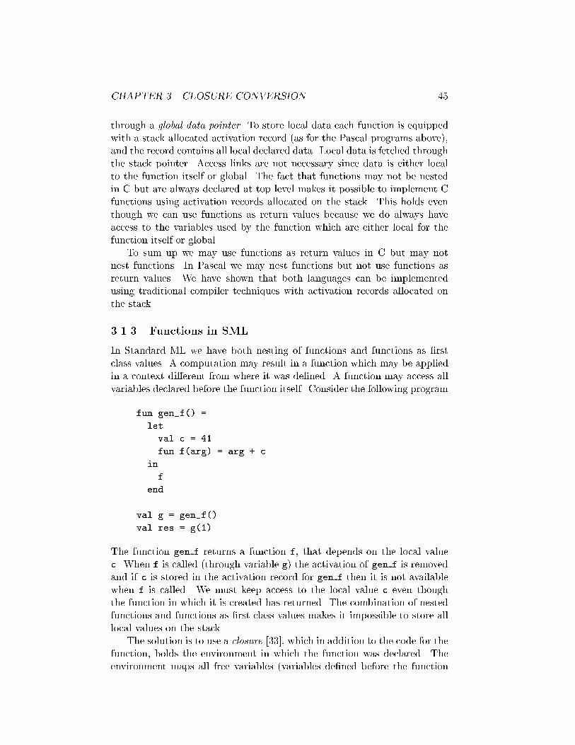
CHAPTER 3. CLOSURE CONVERSION 45
through a global data pointer. To store local data each function is equipped
with a stack allocated activation record (as for the Pascal programs above),
and the record contains all local declared data. Local data is fetched through
the stack pointer. Access links are not necessary since data is either local
to the function itself or global. The fact that functions may not be nested
in C but are always declared at top level makes it possible to implement C
functions using activation records allocated on the stack. This holds even
though we can use functions as return values because we do always have
access to the variables used by the function which are either local for the
function itself or global.
To sum up we may use functions as return values in C but may not
nest functions. In Pascal we may nest functions but not use functions as
return values. We have shown that both languages can be implemented
using traditional compiler techniques with activation records allocated on
the stack.
3.1.3 Functions in SML
In Standard ML we have both nesting of functions and functions as �rst
class values. A computation may result in a function which may be applied
in a context di�erent from where it was de�ned. A function may access all
variables declared before the function itself. Consider the following program
fun gen_f() =
let
val c = 41
fun f(arg) = arg + c
in
f
end
val g = gen_f()
val res = g(1)
The function gen f returns a function f, that depends on the local value
c. When f is called (through variable g) the activation of gen f is removed
and if c is stored in the activation record for gen f then it is not available
when f is called. We must keep access to the local value c even though
the function in which it is created has returned. The combination of nested
functions and functions as �rst class values makes it impossible to store all
local values on the stack.
The solution is to use a closure [33], which in addition to the code for the
function, holds the environment in which the function was declared. The
environment maps all free variables (variables de�ned before the function

CHAPTER 3. CLOSURE CONVERSION 46
itself) to their values. Given the closure (which in general is allocated on
the heap and not on the stack) it is possible to apply the function everywhere
in the program because all information needed to evaluate the function is
held in the closure.
In the above example the function f has c as free variable and the closure
for f is a closure record written: (code
f
; v
c
), where code
f
is a pointer to the
code for f and v
c
is the value of c. When we call f, we fetch the code
pointer from the closure (the �rst element of the closure record) and pass f
the closure record as an argument. The closure record is allocated on the
heap and is accessible for as long time as needed.
1
3.1.4 Uniform Representation of Functions
With functions as �rst class values, it is possible to call several functions
from the same application point. Therefore, a uniform representation of
closures is needed. Consider the program:
fun f(x) =
let
val a = 41
val b = 42
in
if x then
(fn y => y+a)
else
(fn z => z+2*b)
end
val g = f(true) 1 (*1*)
The result function from f(true) called at (*1*) depends on the argument
to f. However, the code performing the call is the same so the two functions
(closures) returned from the if expression must have the same representation.
To call a function we must know where the code for the function is in
addition to the environment needed to evaluate the function (in this case
either a or b). We use the �rst address in the closure for the code pointer
and the following addresses for free variables. The code calling the function
then knows where to jump but not necessarily how the free variables are
organized in the closure which is �ne because they are �rst used in the
body of the called function. The closure records for the two functions are
(code
fny
; a) and (code
fnz
; b). A closure can be viewed as a tuple where
1
In a region based system, region inference decides whether the closure record is al-
located on the stack or on the heap. The point is that the closure record should stay
allocated for as long time as it may be used.

CHAPTER 3. CLOSURE CONVERSION 47
the �rst element is the code pointer and the succeeding elements are free
variables of the function. The arguments y or z are also passed when the
functions are called.
3.1.5 Closure Representation
There are many ways to represent the closures [5, page 112]. We have two
basic methods: at and linked representation and they can be combined in
several ways. We have used at representation in the above examples.
With at representation we copy the free variables into the closure when
the closure is created. This works only if all variables are immutable, (i.e.,
the contents cannot change after declaration). This is indeed the case in
SML contrary to C and Pascal. Consider the program
let
val w=1
fun g(x) =
let
fun f(y) = w+x+y
in
f(42)
end
in
g(3)
end
With linked representation the closure for g contains all free variables in g
(i.e., w) that are not free in the outer function (i.e., still w). The closure for
f contains x (x is not free in g) but not w because w is free in g. Instead we
put a closure pointer to the closure for g in the closure for f and access w
by dereferencing the two closure pointers.
Linked representation works for mutable variables because at any time
there is only one instance of the variable. Flat representation may be
adopted to work with mutuable variables; if there will ever be more than
one instance of a variable it may be implemented as a reference to a cell in
memory.
The at representation tends to create larger closures (i.e., time used on
creation) but optimizes fetching values to only one fetch operation given the
closure pointer. Linked representation minimizes the size of closures and has
better creation times but fetching may now be done through several closure
pointers which is a serious disadvantage. Many combinations of at and
linked representation can be used. Using either at or linked representation
in uence the life range for closure records. With linked representation, a
closure record may be live even though the function it represents is never

CHAPTER 3. CLOSURE CONVERSION 48
called again. This is not the case with at representation. Region inference,
that infers life ranges for closure records, assumes that at representation is
used, thus, we use at rerpesentation in the ML Kit.
3.1.6 A Closure is Not Always Needed
Even though Standard ML (contrary to Pascal) o�ers functions as �rst class
values, functions are not always used as a �rst class value. Actually, it seems
that most functions are used as in Pascal. Consider the program at left.
2
let let
val q = 1 val q = 1
in in
let let
val f = fn x => x + q val f = fn <x,q> => x + q
in in
f 4 (*1*) f <4,q>
end end
end end
The function f does not escape and the free variable q needed to evaluate
f is available at the application point (*1*). It is therefore not necessary
to build a closure for f. Instead we can pass the free variable as an extra
argument to f. We then avoid building a closure and the free variable will
probably be in a machine register in f which is faster that fetching it from a
closure. The above code at right has the free variable q as an extra argument
to f.
The following rules may be used to �nd the function declarations that
do not need to be represented by closures. Let f be the identi�er to which
the function is bound as in the above program.
1. The identi�er f must appear only in applications and only as the
operator, (i.e., f e
2
).
2. All applications of f must have the free variables of f accessible (i.e.,
either as local or free variables in the function containing the applica-
tion).
The �rst rule says that f is a known function, that is, all application points
calling f only call f and the code to jump to is therefore known at compile
time. The second rule makes sure that we can actually access all the free
variables to f at the call site. A variable is accessible in a function g if it is
2
It is important to note that even though the functionality o�ered by Standard ML is
not always used by the programmer then it is still a very important functionality and it
is worth the trouble dealing with.

CHAPTER 3. CLOSURE CONVERSION 49
either a local declared variable or a free variable to g. We have to be a bit
careful, though, because we can nest the declaration of variables and reuse
names. A free variable to f , say v, may be overridden by a more nested
declaration of v which is less nested than the call site. Consider the code at
left:
let let
val free = 42 val free = 42
in in
let let
fun f(x) = free+x fun f<x,free> = free+x
in in
let let
val free = 43 val free = 43
in in
f(2) f <2,free>
end end
end end
end end
If we just pass the variable free to f as an extra argument as in the code at
right then we get 45 and not 44 which is the right result. We must rename
all variables such that variables on the left side of = are di�erent. This has
already been done on RegExp.
The function f in the above program satis�es the two rules but the
mostly nested function g below does not; which rules are not satis�ed?
let
val a = 1
in
let
val g =
let
val b = 2
val g = fn x => a+b+x
in
g
end
in
g 3
end
end
The �rst rule is not satis�ed because the identi�er g is the result in the inner
let expression which is not an application. Rule two is satis�ed even though

CHAPTER 3. CLOSURE CONVERSION 50
it may not seem so. In the application g 3 the free variable b to g is not in
scope. This, however, is not a violation of the rule because g in g 3 is not
the same identi�er as g to which the function is bound.
We need a closure for the inner function bound to the inner g because
it escapes. The closure only has to contain the free variable b because the
application g 3 is in scope of variable a. The code pointer is not needed
because g is the only function which can be applied. There is a variety of
ways to specialize functions as described elsewhere [56].
We note that a function f may still be implemented without a closure
even though there are lambda abstractions in between the declaration of f
and use of f (i.e., f may escape through another function g). Consider the
code:
let
val a = 42
val f = fn x => x - 2 + a
val g = fn x => f x + a
in
g
end
The application to f in the body of g escapes because g escapes. However,
no matter where g is applied, the application to f inside g will always be
to f and the free variable a of f will always be accessible inside g because
a is also free in g. The function g needs to be closure implemented. We
note that if a is not free in g then rule 2 is not satis�ed because a is not
accessible at the call to f.
3.1.7 Region polymorphic functions
A region polymorphic function di�ers from an ordinary function in three
ways [38]:
1. in every application f he
1
; : : : ; e
n
i [a
1
; : : : ; a
m
] a (see Figure 2.5 on
page 22) the function called (e.g., f ) will always be known. It is not
necessary to store the code pointer in the closure for f . The �rst rule
in Section 3.1.6 is always satis�ed.
2. in addition to the ordinary arguments he
1
; : : : ; e
n
i, f also has a region
parameter (i.e., region vector) [a
1
; : : : ; a
n
]
3. region polymorphic functions may be mutually recursive.
Consider the program with g and f as mutually recursive functions.

CHAPTER 3. CLOSURE CONVERSION 51
let
fun g [p1] x = (x+a+f[p1]x)
and f [p2] y = (y+b+f[p2]y + g[p2]y)
in
g[r1]4 + f[r2]5
end
In rule 1 above we noticed that no code pointer is necessary in the closures
for the two functions. The following closures may then be used for the two
functions:
The function g has a and f as free variables: (a; f).
The function f has b, f and g as free variables: (b; f; g).
where f and g are pointers to the two closures respectively. The mutually
recursiveness of the two functions is obvious in the closures. However, the
closures for mutually recursive functions may be merged into one shared
closure [5, 9]. This is possible because the closures are built at the same
time anyway and they have the same lifetime. Merging the two closures
gives the shared closure record : (a; b; f; g): We choose to use shared closures
rather than separate closures.
The next observation is that the two functions f and g may be removed
from the shared closure. There is no need to have the functions f and g
inside the shared closure to point at the same shared closure (i.e., f and g
are not considered free in the body of the functions). The shared closure
record then becomes: (a; b):
We end the discussion about shared closures by looking at how a shared
closure is accessed in di�erent situations [38, page 44]. Let f
1
; : : : ; f
n
be n
mutually recursive functions with bodies e
1
; : : : ; e
n
, respectively, and scope
e. Let the shared closure be sc.
� Accessing any f
i
; i 2 1; : : : ; n yields the same closure sc in e
1
; : : : ; e
n
and e. Now assume an application f
i
he
arg1
; : : : ; e
argn
i [a
1
; : : : ; a
m
] a
directly within e, that is, not within a function in e. This yields the
shared closure sc being built for f
1
; : : : ; f
n
before evaluating e.
� If the application f
i
he
arg1
; : : : ; e
argn
i [a
1
; : : : ; a
m
] a is within e but not
directly within then the shared closure is accessed through the closure
for an in between function (i.e., the shared closure is a free variable of
the in between function).
� Assuming the application f
i
he
arg1
; : : : ; e
argn
i [a
1
; : : : ; a
m
] a is directly
within e
i
; i 2 1; : : : ; n then the shared closure bound to f
i
is the same
as the current one, (i.e., no code is needed to �nd the closure).

CHAPTER 3. CLOSURE CONVERSION 52
3.1.8 Closure Explication
Several compilers, including the former versions of the ML Kit, decides the
representation of closures at the time they compile from lambda calculus (or
continuation passing style) into machine code (i.e., during code generation).
However, it is possible to separate the representation of closures (closure
conversion) from other compilation tasks because the representation of clo-
sures is not machine dependent and it is not di�cult to express closures
explicitly in intermediate languages.
There are several advantages of representing closures explicitly. Code
generation becomes simpler because all functions are at top level exactly as
they will be after code generation. Moreover, it is advantageous to include
machine independent information in the intermediate languages because it
gives more information for the optimizations performed in the backend.
We have implemented a closure conversion phase in the ML Kit that
converts the RegExp language into a language called ClosExp where function
declarations are substituted for closures being the values of the functions.
Furthermore, we give each function the closure as an explicit argument and
all accesses to values in the closure are changed into selects into the closure.
We also make the region vectors explicit in the program. There are no free
variables in the functions after closure conversion and they can be lifted to
top level.
3
The program has been translated from one expression into a list
of function declarations. Having closures made explicit in ClosExp makes
the succeeding phases, including code generation, simpler and we have made
it possible (though not used yet) to apply more advanced analyses on the
representation of closures.
3.2 Calculating the Need For Closures
In this section we present the algorithm that �nds the functions (either
ordinary or letrec bound) that may be implemented without a closure,
that is, with all free variables passed as arguments.
We use the two rules laid out in Section 3.1.6 and the additional re-
quirement that the maximum number of free variables may at most be
max free args . The limit max free args makes sure that we do not pass
huge closures as arguments where the total number of arguments exceeds
the number of machine registers available. The number max free args de-
pends on the register allocator used. If the closure arguments have to be
passed on the stack anyway then it is likely that it is better to build the
closure in order to limit the register pressure.
The algorithm performs a forward scan of the RegExp expression and
3
Variables imported in the module may still be considered free but they are referenced
through a global label.

CHAPTER 3. CLOSURE CONVERSION 53
computes a partially de�ned function
fe 2 FE = LamVar ! ffn free list ; fix free listg:
Given a variable f to which a function is bound then if f is not in the
domain of fe then the function bound to f should be implemented with a
closure. If f is in the domain of fe then it may be implemented without a
closure and fe(f) gives the free variables of the function. We let fn denote
ordinary functions and fix denote letrec bound functions.
At application points we need to make sure that the free variables of
the called function are accessible (rule two). The accessible variables are
recorded in a variable environment
VE = RegVar [ LamVar
The algorithm uses two return types
rtnType ::= func free list j other
We let RtnType denote the set of return types. If a subexpression evaluates
to a function then the return type is func and otherwise the return type is
other. Consider the expression:
let
val f = fn x => x+2
in
e
end
The return type returned from expression fn x => x+2 is func and we insert
the relation f 7! func in fe.
The algorithm inserts a function in fe when the function is declared. The
function is removed from fe if one of the requirements are not satis�ed.
Algorithm F does one forward traversal of the program.
F : RegExp ! FE ! VE ! FE � RtnType seq
3.2.1 Variables and Constants
F [[x]] fe ve =
if x 2 dom(fe) then
(fe n fxg, hotheri)
else
(fe, hotheri)
The algorithm handles applications speci�cally so the variable x in the above
case will always appear as a use, that is, not as an operator in an application.
If x represents a function then x has to be implemented with a closure and
is therefore removed from fe (i.e., rule one).

CHAPTER 3. CLOSURE CONVERSION 54
F [[i ]] fe ve = (fe, hotheri)
F [[nil]] fe ve = (fe, hotheri)
3.2.2 Boxed Expressions
F [[(e
1
; : : : ; e
n
) a]] fe
0
ve =
let
val (fe
i
, ) = F [[e
i
]] fe
i�1
ve i = 1; : : : ; n
in
(fe
n
, hotheri)
end
If e
i
for some i 2 1; : : : ; n evaluates to a function then the function is im-
plemented with a closure because it is stored in the record.
F [[�
free
hx
1
; : : : ; x
n
i => e a]] fe ve =
let
val (fe
0
, ) = F [[e]] fe (setof(free) [ fx
1
; : : : ; x
n
g)
in
(fe
0
, hfunc freei)
end
The function setof converts the list of variables into a set of variables.
The set of accessible variables in the body of the function is precisely the
arguments and the free variables of the function. The return type is a
function indicated by func.
3.2.3 Expressions
The interesting cases are the let, letrec and application constructs.
Constructors
F [[:: e]] fe ve = F [[e]] fe ve
Binary Operations
F [[e
1
bop e
2
]] fe ve =
val (fe
1
, ) = F [[e
1
]] fe ve
val (fe
2
, ) = F [[e
2
]] fe
1
ve
in
(fe
2
, hotheri)
end
The result of a binary operation is an integer so the return type is other.

CHAPTER 3. CLOSURE CONVERSION 55
Selection
F [[#n(e)]] fe ve = F [[e]] fe ve
If #n(e) evaluates to a function then the function is closure implemented
(i.e., the function is bound to a variable that has been used in an expression
creating a record.)
letrec bound functions
F [[letrec f
free
hx
1
; : : : ; x
n
i [�
1
: m
1
; : : : ; �
l
: m
l
] a = e
1
in e
2
end]] fe ve =
let
val fe
0
= if jfreej < max free args then
fe + ff 7! (fix free)g
else
fe
val (fe
0
, ) = F [[e
1
]] fe
0
(setof(free) [ ff; x
1
; : : : ; x
n
; �
1
; : : : ; �
l
g)
in
F [[e
2
]] fe
0
(ve [ ffg)
end
Initially we assume f not to be closure implemented by inserting f into fe
i� the number of free variables is less than max free args . If f should be
closure implemented then f is removed from fe when computing e
1
and e
2
.
The function f is accessible in both e
1
and e
2
. The function j�j : � list ! Int
computes the number of elements in a list.
Applications
Ordinary applications and letrec applications are handled similarly. The
letrec application is:
F [[f e [a
1
; : : : ; a
m
] a]] fe ve =
let
val fe
0
= if (f 2 dom(fe) and
fe(f).free � ve) then
fe
else
fe n ffg
val (fe
0
, ) = F [[e]] fe
0
ve
in
(fe
0
, hotheri)
end
If fe(f) = ( free list), then we write fe(f).free for free. The second re-
quirement in the condition ensures that all free variables are accessible at

CHAPTER 3. CLOSURE CONVERSION 56
the application point (i.e., rule two). The return type is hotheri because a
function is not declared.
Letregion
F [[letregion � : m in e end]] fe ve =
F [[e]] fe (ve + f�g)
The region variable � is accessible in the body e.
Declaring variables
F [[he
1
; : : : ; e
n
i]] fe
0
ve =
let
val (fe
i
,rtn type
i
) = F [[e
i
]] fe
i�1
ve i = 1; : : : ; n
in
(fe
n
, hrtn type
1
; : : : ; rtn type
n
i)
end
The set of accessible variables in each sub expression e
i
is the same because
no variable is declared between the sub expressions. We use the newest
environment fe in each sub expression because if a function has to be imple-
mented with a closure in one of the sub expressions then it has to be deleted
from the fe that we return.
F [[let val hx
1
; : : : ; x
n
i = e
1
in e
2
end]] fe ve =
let
val (fe
0
,hrtn type
1
; : : : ; rtn type
n
i) = F [[e
1
]] fe ve
val fe
i
= case rtn type
i
of i = 1; : : : ; n
func free => fe
i�1
+ fx
i
7! (fn free)g
| other => fe
i�1
in
F [[e
2
]] fe
n
(ve + fx
1
; : : : ; x
n
g)
end
The functions (if any) bound to a variable x
i
are inserted into fe as an
ordinary function fn. The variables x
1
; : : : ; x
n
are distinct.
Case
F [[case e
1
of c => e
2
| => e
3
]] fe ve =
let
val (fe
1
, ) = F [[e
1
]] fe ve
val (fe
2
, ) = F [[e
2
]] fe
1
ve
val (fe
3
, ) = F [[e
3
]] fe
2
ve

CHAPTER 3. CLOSURE CONVERSION 57
in
(fe
3
,hotheri)
end
F [[case e
1
of ::x => e
2
| => e
3
]] fe ve =
let
val (fe
1
, ) = F [[e
1
]] fe ve
val (fe
2
, ) = F [[e
2
]] fe
1
(ve+fxg)
val (fe
3
, ) = F [[e
3
]] fe
2
ve
in
(fe
3
,hotheri)
end
If e
2
or e
3
return a function then the function has to be implemented with a
closure because the application sites do not know which function is applied.
The return type is therefore other.
3.3 ClosExp
In this section we present ClosExp which is a re�nement of RegExp where
functions are lifted to top level. ClosExp is the result of closure conversion.
3.3.1 Call convention
A call convention speci�es how arguments to a function are passed. We use
a call convention with �ve entries:
cc = fclos: LamVar option,
free: LamVar list,
args: LamVar list,
reg vec: LamVar option,
reg args:LamVar list g
A function f may either have its free variables passed in a closure or as extra
arguments. If a closure is used then the closure is passed as an argument
to the function and the closure argument is written in the clos entry. If a
closure is not used then the free variable arguments are written in the entry
free. It is possible, in the same call, to pass some of the free variables in free
variable arguments and some of the free variables in a closure argument.
However, we do not use that option, that is, the entry clos and the entry
free cannot, at the same time, be non empty.
Regular arguments are written in the entry args. As with free variables
we can either pass region variables in a region vector or as region variable
arguments. We always pass region variables in a region vector argument

CHAPTER 3. CLOSURE CONVERSION 58
and the region vector argument is written in the entry reg vec. The entry
reg args is never used and is included in the call convention for complete-
ness. It is likely that we, in the future, may extend the call conventions to
include functions receiving region variables as extra arguments and thereby
eliminate the need for a region vector; this is especially useful for functions
with a low register pressure.
We note that a list may be empty (see Figure 2.4) and LamVar option
means that either there is a variable or not.
The call convention is designed to maximize exibility in calling func-
tions. The call convention fully describes how both ordinary and letrec
functions are called. The closure conversion phase lifts all functions to top
level and with the call convention speci�ed above we get the following gram-
mar for top level declarations:
top decl ::= �
fun
lab
cc => e
j �
fn
lab
cc => e
The two constructs are identical except that we syntactically di�erentiate
between letrec (abbreviated fun) and ordinary functions (abbreviated fn).
The label lab is a unique ident (name) for the function; lab 2 Label. We
let the set TopDecl denote the set of top level declarations ranged over by
top decl.
The order of arguments passed to the function is uniquely determined by
the register allocator that allocates the variables to either machine registers
or the machine stack.
Application points must follow the call convention for the called function.
We use the following grammar at application points:
e ::= e
ck
he
1
; : : : ; e
n
i he
clos
i he
f
1
; : : : ; e
f
m
i
j lab
ck
he
1
; : : : ; e
n
i he
reg
i he
�
1
; : : : ; e
�
l
i he
clos
i he
f
1
; : : : ; e
f
m
i
For ordinary function calls the regular arguments e
1
; : : : ; e
n
are written
in the �rst bracket and the optional closure and free values in the second
and third bracket. We never use the second and third bracket at the same
time.
The letrec application is similar except that the region vector and re-
gion values have been squeezed in as the second and third bracket. We
note that ClosExp is in K{normal form and all values are either bound to a
variable ranged over by x and f or the value is a constant.
In examples, we only write the non empty entries in a call convention.
We did not write the region vector that we reuse in the recursive call to
gen list in the example on page 38. In ClosExp we explicitly write all the
arguments.

CHAPTER 3. CLOSURE CONVERSION 59
3.3.2 Functions
Now that all functions are lifted to top level the two expressions
�
free
hx
1
; : : : ; x
n
i => e
and
letrec f
free
hx
1
; : : : ; x
n
i [b
1
; : : : ; b
m
] a = e in e end
disappear from the grammar.
Instead of the � expression we introduce a new boxed expression:
be ::= �
lab
[e
f
1
; : : : ; e
f
n
]
that evaluates to a closure record: (lab; v
f
1
; : : : ; v
f
n
) where v
f
i
is the value
of e
f
i
, i = 1; : : : ; n. The label lab refers to the function at top level.
The letrec construct is replaced by three new constructs. The boxed
expressions
be ::= [a
1
; : : : ; a
n
]
regvec
j [e
f
1
; : : : ; e
f
n
]
sclos
are the region vector and shared closure respectively. They evaluate to a
region vector record (v
�
1
; : : : ; v
�
n
) and a shared closure record (v
f
1
; : : : ; v
f
n
).
We also need a letrec construct to make the scope for f explicit.
e ::= letrec f
lab
= be a in e end
The label lab connects the top level function �
fun
lab
with f . We often omit the
label in examples where f and the label are identical. The boxed expression,
be, is always a shared closure which is bound to the variable f .
Examples
Consider the RegExp program:
let
val b = 5
val f = �
fbg
hxi =>
(let
val fn y = (�
fb;xg
hyi => x + y + b) attop r1
in
fn y
end) attop r1
in
f
fncall
h5i
end
In ClosExp we write the same program as:

CHAPTER 3. CLOSURE CONVERSION 60
�
fn
main
f g => let
val b = 5
val f = �
fn x
[b] attop r1
in
f
fncall
h5i hf i hi
end
�
fn
fn x
fclos=c, args=[x]g =>
let
val fn y = �
fn y
[#1(c), x] attop r1
in
fn y
end
�
fn
fn y
fclos=c, args=[y]g => #2(c) + y + #1(c)
Three functions are created at top level where main is the function that
initiates computation. All functions are closed because access to arguments
and free variables are described in the call convention. We insert explicit
selections into the closure records. The closure record passed to fn y is
c =(fn y ; b; x) where fn y is the code label and the expression #2(c) denotes
x in the original program and #1(c) denotes b. The closure record for fn x
is c =(fn x ; b).
We note that ClosExp is not a typed intermediate language. However,
it is possible to give the closure record for fn y a simple type, for instance:
c : Code � Int � Int where Code is a type donoting code. It would greatly
improve the reliability of the compiler if the intermediate languages could
be type checked even though the type system might not be sound, that is,
we cannot prove that the source and translated program evaluate to the
same result even though the translated program type checks. It is also
possible to engineer sound type systems where we can prove that if the
closure converted program type checks then it evaluates to the same result
as the original program [36]. Unfortunately, this is beyond the scope of this
project.
The running example for the next chapters is shown below:
fun foldl f b xs =
case xs of
[] => b
| x::xs' => foldl f (f x b) xs'
The same program in RegExp is shown in Figure 3.3.
The translation to ClosExp is shown in Figure 3.4 and Figure 3.5. Four
top level functions are created.

CHAPTER 3. CLOSURE CONVERSION 61
letrec foldl
[ ]
hfi [r7 : 4; r8 : 4] attop r1 =
let
val fn b = �
[f;r8;foldl]
hbi attop r7 =>
let
val fn xs = �
[b;f;foldl]
hxsi attop r8 =>
(case xs of
nil => b
| :: (v942 ) =>
let
val x = #0(v942 )
val xs' = #1(v942 )
in
letregion r22 :4 in
let
val k80 =
letregion r24 :4 in
let
val k77 =
letregion r25 :2 in
foldl
funcall
hfi [atbot r24; atbot r22] atbot r25
end (*r25*)
val k79 =
let
val k78 = f
fncall
hxi
in
k78
fncall
hbi
end (*let*)
in
k77
fncall
k79
end (*let*)
end (*r24*)
in
k80
fncall
hxs' i
end (*let*)
end (*r22*)
end (*let*))
in
fn xs
end (*let*)
in
fn b
end (*let*)
in
foldl
funcall
hsumi [atbot r4; atbot r5] atbot r6
end (*letrec*)
Figure 3.3: Our running example program written in RegExp. We
assume sum, r1, r4, r5 and r6 to be previously de�ned. We have k77 =
foldl f , k78 = f x, k79 = f x b and k80 = foldl f (f x b).

CHAPTER 3. CLOSURE CONVERSION 62
�
fun
foldl
fargs=[f ], recvec=rv , clos=cg =>
let
val fn b = �
fn b
[f , #1(rv), c] attop ff #0(rv)
in
fn b
end
�
fn
fn b
fargs=[b], clos=cg =>
let
val fn xs = �
fn xs
[b, #1(c), #3(c)] attop ff #2(c)
in
fn xs
end
�
fn
main
f g =>
letrec foldl
foldl
= [ ]
sclos
attop li r1
in
let
val rv = [attop lf r4 , atbot lf r5 ]
regvec
atbot lf r6
in
foldl
funcall
hsumi hrvi hi hfoldl i hi
end
end
Figure 3.4: The �rst three top level functions in our running example
program translated into ClosExp. In the letrec binding we introduce
both the label foldl and the variable foldl (holding the empty shared
closure). In the application the �rst term foldl is the label and the shared
closure is accessed in the fourth bracket. Actually the shared closure is
empty so it should be omitted and will be in the implementation. The
closure record c for fn b is (fn b, f , r5, foldl ).

CHAPTER 3. CLOSURE CONVERSION 63
�
fn
fn xs
fargs=[xs], clos=cg =>
(case xs of
nil => #1(c)
| :: (v942 ) =>
let
val x = #0(v942 )
val xs' = #1(v942 )
in
letregion r22 :4 in
let
val k80 =
letregion r24 :4 in
let
val k77 =
letregion r25 :2 in
let
val rv = [atbot lf r24 , atbot lf r22 ] atbot lf r25
in
foldl
funcall
h#2(c)i hrvi hi h#3(c)i hi
end
end (*r25*)
val k79 =
let
val k78 = #2(c)
fncall
hxi h#2(c)i hi
in
k78
fncall
h#1(c)i hk78 i hi
end (*let*)
in
k77
fncall
hk79 i hk77 i hi
end (*let*)
end (*r24*)
in
k80
fncall
hxs' i hk80 i hi
end (*let*)
end (*r22*)
end (*let*))
Figure 3.5: The main function fn xs. The label in the call to foldl is
known at compile time and is therefore not free in the function, however,
the shared closure foldl is free in the function. The closure record c is
(fn xs, b, f , foldl ).

CHAPTER 3. CLOSURE CONVERSION 64
3.3.3 Storage Modes
We extend the set of storage modes, see Section 2.5, in order to make code
generation easier, see Chapter 9. The storage modes attop, atbot and sat
are replaced by eight storage modes:
attop ff attop fi
attop lf attop li
atbot lf atbot li
sat ff sat fi
We have added the letter combinations:
ff: a formal region parameter with finite multiplicity.
fi: a formal region parameter with in�nite multiplicity.
lf: a letregion bound region variable with finite multiplicity.
li: a letregion bound region variable with in�nite multiplicity.
Consider the allocation point: e attop ff �. The storage mode attop ff
says that region variable � is bound as a formal region parameter with �nite
multiplicity. The new storage modes do not add new information to the
program but moves the information to places where the information is used
by the code generator. Knowing how a region variable is bound and its
multiplicity at the application point makes code generation easier. The set
SMA is the set of storage mode annotations ranged over by sma.
The function resolve sm de�ned on page 35 is rede�ned to work on the
new storage modes:
resolve sm: StorageMode � SMA! StorageMode
resolve sm( , atbot lf) = atbot
resolve sm( , atbot li) = atbot
resolve sm( , attop ff) = attop
resolve sm( , attop fi) = attop
resolve sm( , attop lf) = attop
resolve sm( , attop li) = attop
resolve sm(atbot, sat ff) = atbot
resolve sm(atbot, sat fi) = atbot
resolve sm(attop, sat ff) = attop
resolve sm(attop, sat fi) = attop
3.3.4 Grammar for ClosExp
The grammar for ClosExp is shown in Figure 3.6 and semantic objects for
the grammar in Figure 3.7.
For ordinary applications, e
ck
is either a closure or a label. For letrec
applications we always know which function to call. We let the set CC

CHAPTER 3. CLOSURE CONVERSION 65
denote call conventions. The translation into ClosExp (Section 3.4.3) intro-
duces extra let bindings and it is possible that a region descriptor is bound
to a lambda variable lv and not a region variable �. This happens when
region descriptors are stored in region vectors and then selected from the
region vectors or simply appear as a free variable to the function. We let
the set ClosExp be the set of expressions ranged over by e.
3.3.5 Dynamic Semantics for ClosExp
The semantic objects used in the dynamic semantics for ClosExp is shown
in Figure 3.8. A region name rn is used to identify a region in the heap. A
region descriptor contains the region name together with the multiplicity and
storage mode. We have turned a region descriptor into a value because they
are stored in region records. Because region descriptors are values we have
no need for the region environment RE as used in the dynamic semantics
for RegExp. Note the di�erence between a storage mode sm and a storage
mode annotation sma de�ned in the grammar, Figure 3.6. A storage mode
is either atbot or attop and never somewhere{at. A label lab is considered
a constant used when calling functions.
Top level declarations FE ` top decl ) FE
0
We create a function environment FE containing all the functions declared
at top level.
FE ` �
fun
lab
cc => e) FE + flab 7! hcc; eig
(3.1)
FE ` �
fn
lab
cc => e) FE + flab 7! hcc; eig
(3.2)
FE ` top decl
1
) FE
1
FE
1
` top decl
2
) FE
2
FE ` top decl
1
; top decl
2
) FE
2
(3.3)
Begin evaluation st; h;E ` e) v; h
0
To start evaluation we call the function main with an empty call convention.
The stack and heap are empty. The function environment FE is obtained
from the top level declarations.
fg; fg; (fg;FE) ` main
fncall
hi hi hi ) v; h
0
(3.4)

CHAPTER 3. CLOSURE CONVERSION 66
top decl ::= �
fun
lab
cc => e
j �
fn
lab
cc => e
j top decl
1
; top decl
2
ck ::= funjmp j funcall j fnjmp j fncall
sma ::= attop li j attop lf j attop fi j attop ff
j atbot li j atbot lf j sat fi j sat ff
a ::= sma xv
m ::= n j 1
b ::= � : m
c ::= i j nilj lab
pat ::= c j :: x
bop ::= +; -; <; : : :
be ::= (e
1
; : : : ; e
n
)
j �
lab
[e
f
1
; : : : ; e
f
n
]
j [a
1
; : : : ; a
n
]
regvec
j [e
f
1
; : : : ; e
f
n
]
sclos
e ::= x
j be a
j c
j :: e
j e
1
bop e
2
j #n(e)
j letrec f
lab
= be a in e end
j e
ck
he
1
; : : : ; e
n
i he
clos
i he
f
1
; : : : ; e
f
m
i
j lab
ck
he
1
; : : : ; e
n
i he
reg
i ha
�
1
; : : : ; a
�
l
i he
clos
i he
f
1
; : : : ; e
f
m
i
j letregion b in e end
j let val hx
1
; : : : ; x
n
i = e
1
in e
2
end
j case e
1
of pat => e
2
| => e
3
j he
1
; : : : ; e
n
i
Figure 3.6: The grammar for ClosExp. The call convention cc is de�ned
in Section 3.3.1. Note that an allocation point a may be of the form sma
� and sma lv.

CHAPTER 3. CLOSURE CONVERSION 67
top decl 2 TopDecl
e 2 ClosExp
x; f; lv 2 LamVar
lab 2 Label
i 2 Int
� 2 RegVar
cc 2 CC
xv 2 Var = LamVar [ RegVar
Figure 3.7: The semantic objects used in ClosExp. We let CC denote
the set of call conventions.
st 2 Stack = RegDesc stack
h 2 Heap = RegName ! Reg
s 2 Store = Stack �Heap
rd 2 RegDesc = RegName �Mult � StorageMode
rn 2 RegName
r 2 Reg = O�set ! BoxedVal
o 2 O�set
bv 2 BoxedVal = Record
ubv 2 UnBoxedVal = Int [ fnilg [ ::(Val) [ Label
v 2 Val = Addr [UnBoxedVal [ RegDesc
rec 2 Record = Val� : : :�Val
(rd; o) 2 Addr = RegName �O�set
m 2 Mult = Int [ f1g
sm 2 StorageMode = fatbot; attopg
hcc; ei 2 FEelem = (CC� ClosExp)
VE = Var ! Val
FE = Label ! FEelem
E = SClos = VE � FE
Figure 3.8: The semantic objects used in the dynamic semantics of
ClosExp. The function environment FE maps labels into a call conven-
tion cc 2 CC and the code for the function. The record rec is used for
ordinary records, closure records and region records.

CHAPTER 3. CLOSURE CONVERSION 68
Constants ` ubv) ubv
` i) i
(3.5)
` nil) nil
(3.6)
` lab) lab
(3.7)
We have the constants: integers (i), nil and labels lab. They all create
an unboxed value.
Allocation Points st; h;E ` a) (rn; o); h
0
VE(xv) = (rn;m; sm)
resolve sm(sm; sma) = attop
o 62 dom(h(rn))
st; h; (VE;FE) ` sma xv ) (rn; o); h
(3.8)
VE(xv) = (rn;m; sm)
resolve sm(sm; sma) = atbot
h
0
= h+ frn 7! fgg
o 62 dom(h(rn))
st; h; (VE;RE) ` sma xv ) (rn; o); h
0
(3.9)
If we allocate atbot then the heap is updated with the region xv being
reset. The function resolve sm is de�ned on page 64.
Call Conventions st; h;E `
ap
e) hcc; e
0
i; h
0
st; h;E ` e) (rn; o); h
0
h
0
(rn; o) = (lab; v
1
; : : : ; v
n
)
FE(lab) = hcc; e
0
i
st; h;E `
ap
e) hcc; e
0
i; h
0
(3.10)
FE(lab) = hcc; ei
st; h;E `
ap
lab ) hcc; ei; h
(3.11)

CHAPTER 3. CLOSURE CONVERSION 69
The �rst rule covers closure implemented functions and the second rule
known functions. The call convention and body of function is looked up in
FE.
We have a rule that matches arguments with a call convention and re-
turns a variable environment where arguments in the call convention are
mapped into the argument values.
st; h
i�1
;E ` e
i
) v
i
; h
i
i = 1; : : : ; l
cc = fargs = [x
1
; : : : ; x
n
];
reg vec = x
n+1
;
reg args = [x
n+2
; : : : ; x
m
];
clos = x
m+1
;
free = [x
m+2
; : : : ; x
l
]g
VE
0
= fx
i
7! v
i
g
i=1;::: ;l
st; h
0
;E `
cc
(cc; he
1
; : : : ; e
n
i he
n+1
i he
n+2
; : : : ; e
m
i
he
m+1
i he
m+2
; : : : ; e
l
i)) VE
0
; h
l
(3.12)
It is not mandatory that all brackets are non empty as long as the call
convention matches the supplied arguments. For instance, if a region record
is passed as argument then there must be a corresponding variable in the
call convention.
Boxed Expressions st; h;E ` be) bv; h
0
st; h
i�1
;E ` e
i
) v
i
; h
i
i = 1; : : : ; n
st; h
0
;E ` (e
1
; : : : ; e
n
)) (v
1
; : : : ; v
n
); h
n
(3.13)
st; h
i�1
;E ` e
f
i
) v
f
i
; h
i
i = 1; : : : ; n
st; h
0
;E ` �
lab
[e
f
1
; : : : ; e
f
n
]) (lab; v
f
1
; : : : ; v
f
n
); h
n
(3.14)
VE(xv
i
) = (rn
i
;m
i
; sm
i
)
sm
0
i
= resolve sm(sm
i
; sma
i
) i = 1; : : : ; n
st; h; (VE;FE) ` [sma
1
xv
1
; : : : ; sma
n
xv
n
]
regvec
)
((rn
1
;m
1
; sm
0
1
); : : : ; (rn
n
;m
n
; sm
0
n
)); h
(3.15)
st; h
i�1
;E ` e
f
i
) v
f
i
; h
i
i = 1; : : : ; n
st; h
0
;E ` [e
f
1
; : : : ; e
f
n
]
sclos
) (v
f
1
; : : : ; v
f
n
); h
n
(3.16)
An ordinary function closure (rule 3.14) has the function label as �rst
component in the closure. A shared closure (rule 3.16) does not have labels
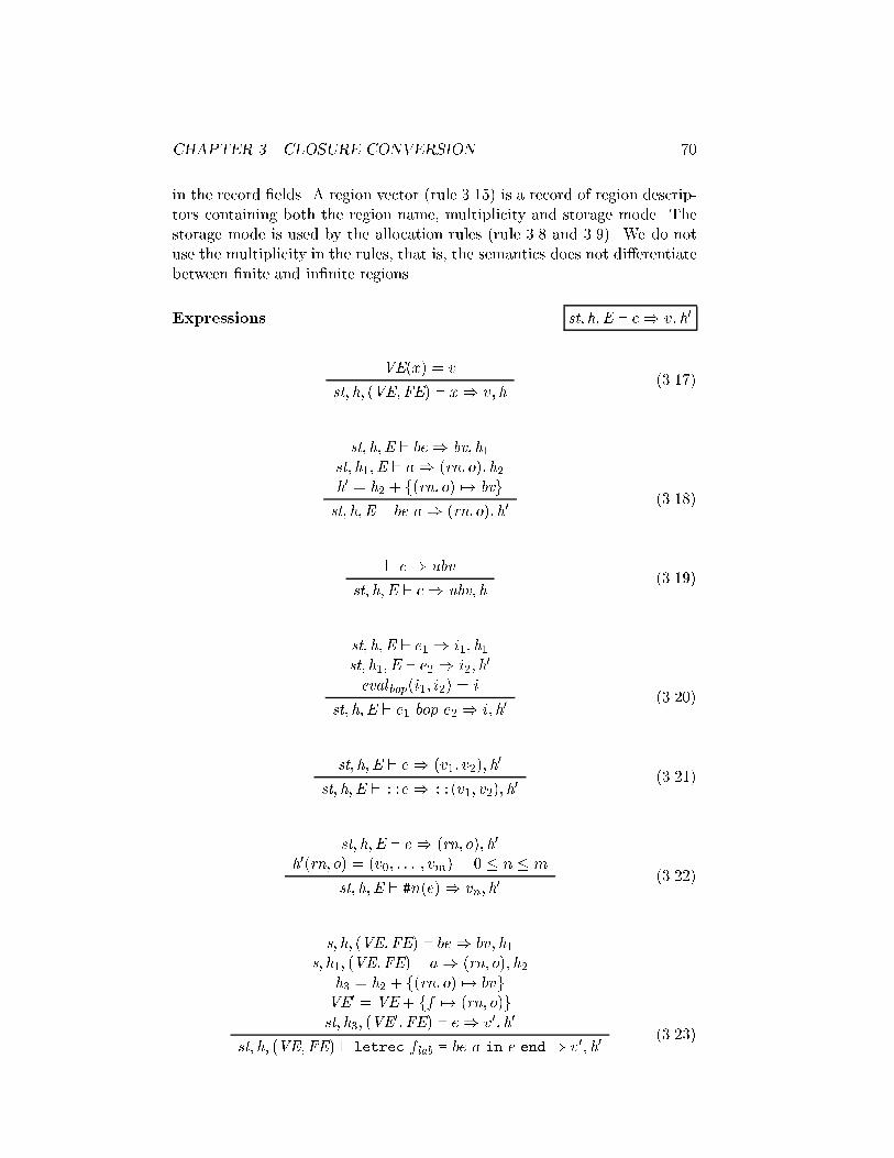
CHAPTER 3. CLOSURE CONVERSION 70
in the record �elds. A region vector (rule 3.15) is a record of region descrip-
tors containing both the region name, multiplicity and storage mode. The
storage mode is used by the allocation rules (rule 3.8 and 3.9). We do not
use the multiplicity in the rules, that is, the semantics does not di�erentiate
between �nite and in�nite regions.
Expressions st; h;E ` e) v; h
0
VE(x) = v
st; h; (VE;FE) ` x) v; h
(3.17)
st; h;E ` be) bv; h
1
st; h
1
;E ` a) (rn; o); h
2
h
0
= h
2
+ f(rn; o) 7! bvg
st; h;E ` be a) (rn; o); h
0
(3.18)
` c) ubv
st; h;E ` c) ubv; h
(3.19)
st; h;E ` e
1
) i
1
; h
1
st; h
1
;E ` e
2
) i
2
; h
0
eval
bop
(i
1
; i
2
) = i
st; h;E ` e
1
bop e
2
) i; h
0
(3.20)
st; h;E ` e) (v
1
; v
2
); h
0
st; h;E ` ::e) ::(v
1
; v
2
); h
0
(3.21)
st; h;E ` e) (rn; o); h
0
h
0
(rn; o) = (v
0
; : : : ; v
m
) 0 � n � m
st; h;E ` #n(e)) v
n
; h
0
(3.22)
s; h; (VE;FE) ` be) bv; h
1
s; h
1
; (VE;FE) ` a) (rn; o); h
2
h
3
= h
2
+ f(rn; o) 7! bvg
VE
0
= VE+ ff 7! (rn; o)g
st; h
3
; (VE
0
;FE) ` e) v
0
; h
0
st; h; (VE;FE) ` letrec f
lab
= be a in e end) v
0
; h
0
(3.23)

CHAPTER 3. CLOSURE CONVERSION 71
st; h;E `
ap
e
ck
) hcc; e
0
i
st; h; (VE;FE) `
cc
(cc; h~ei hi hi he
clos
i h ~e
f
i)) VE
0
; h
1
st; h
1
; (VE
0
;FE) ` e
0
) v
0
; h
0
st; h; (VE;FE) ` e
ck
h~ei he
clos
i h ~e
f
i ) v
0
; h
0
(3.24)
st; h;E `
ap
lab
ck
) hcc; e
0
i
st; h; (VE;FE) `
cc
(cc; h~ei he
reg
i h~e
�
i he
clos
i h ~e
f
i)) VE
0
; h
1
st; h
1
; (VE
0
;FE) ` e
0
) v
0
; h
0
st; h; (VE;FE) `
lab
ck
h~ei he
reg
i h~e
�
i he
clos
i h ~e
f
i ) v
0
; h
0
(3.25)
rn 62 dom(h)
h
1
= h+ frn 7! fgg
st
1
= push(st; rn)
st
1
; h
1
; (VE+ f� 7! (rn;m; attop)g;FE) ` e) v
0
; h
2
( ; st) = pop(st
1
)
h
0
= h
2
n frng
st; h; (VE;FE) ` letregion � : m in e end) v
0
; h
0
(3.26)
st; h; (VE;FE) ` e
1
) hv
1
; : : : ; v
n
i; h
1
st; h
1
; (VE+ fx
i
7! v
i
g
i=1;::: ;n
;FE) ` e
2
) v
0
; h
0
st; h; (VE;FE) ` let val hx
1
; : : : ; x
n
i = e
1
in e
2
end) v
0
; h
0
(3.27)
st; h
i�1
;E ` e
i
) v
i
; h
i
i = 1; : : : ; n
st; h
0
;E ` he
1
; : : : ; e
n
i ) hv
1
; : : : ; v
n
i; h
n
(3.28)
st; h; (VE;FE) ` e
1
) ::(v); h
1
st; h
1
; (VE+ fx 7! vg;FE) ` e
2
) v
0
; h
0
st; h; (VE;FE) ` case e
1
of ::x => e
2
| => e
3
) v
0
; h
0
(3.29)
st; h;E ` e
1
) c; h
1
st; h
1
;E ` e
2
) v
0
; h
0
st; h;E ` case e
1
of c => e
2
| => e
3
) v
0
; h
0
(3.30)
st; h;E ` e
1
) c
0
; h
1
c
0
6= c
st; h
1
;E ` e
3
) v
0
; h
0
st; h;E ` case e
1
of c => e
2
| => e
3
) v
0
; h
0
(3.31)

CHAPTER 3. CLOSURE CONVERSION 72
st; h;E ` e
1
) nil; h
1
st; h
1
;E ` e
3
) v
0
; h
0
st; h;E ` case e
1
of ::x => e
2
| => e
3
) v
0
; h
0
(3.32)
A boxed expression (rule 3.18) is allocated in a region.
Binary operations (rule 3.20) work on integers only. As for RegExp, we
use the function eval
bop
: Int � Int! Int to evaluate the function bop given
the two integer arguments.
In the letrec rule (rule 3.23) the boxed expression (be) is always a
shared closure.
Rule 3.24 covers the unknown function calls. The three sets of arguments
are evaluated and bound in the environment VE
0
(rule 3.12) before the body
of the called function is evaluated. The arguments and call convention must
match.
The rule for known applications (rule 3.25) is similar to the rule for
unknown applications except that we have �ve sets of arguments and not
three. Rule 3.12 is used to match the call convention and arguments.
Rule 3.26 allocates a fresh region, sets the multiplicity to m and storage
mode to attop. The storage mode is chosen arbitrarily because it is ex-
plicitly set at the allocation points and when building a region vector (rule
3.15).
3.4 Closure conversion
The algorithm that translates RegExp into ClosExp (C) is fairly straight-
forward. However, there are a few minor points that we address before we
present C:
3.4.1 Preserve K-normal form
In order to keep the code generator simple we want all value creating ex-
pressions to be assigned a variable (i.e., preserve the K{normal form). If
we keep ClosExp and LineExp (see Chapter 4) in K{normal form and all
value creating expressions are atomic then we do not have to introduce more
variables during code generation. We can generate code without introduc-
ing temporary variables as long as all value creating expressions are atomic.
An atomic expression is an expression that may easily be implemented in
machine code (maybe with the use of a few machine registers). All value cre-
ating expressions in ClosExp are atomic expressions. The simpli�cation of
function declaration and application in ClosExp is essential for this property
to hold.
The ClosExp program in Figure 3.4 and 3.5 is not in K{normal form.
For instance, in Figure 3.5 line 19, we have a call to foldl . The closure for

CHAPTER 3. CLOSURE CONVERSION 73
foldl is stored as component number 2 in the closure variable c (i.e., #2(c)).
To be in K{normal form we need the invariant that all uses in an expression
are either a variable or a constant. If this is not true then we cannot in
general generate code for the expression with no additional variables to hold
the result of sub expressions.
The algorithm C must translate the application into
let
val rv = [atbot r24 , atbot r22 ] atbot r25
val lv = #2(c)
in
foldl
funcall
hlvi hrvi hi hfoldli hi
end
where lv is a fresh lambda variable.
3.4.2 Call Conventions
The algorithm C assigns call conventions to functions using the function FE
computed in Section 3.2.3.
Consider a RegExp function
�
[f
1
;::: ;f
m
]
hx
1
; : : : ; x
n
i => e
with free variables f
1
; : : : ; f
m
. If the function is closure implemented then
we create a ClosExp closure:
�
lab
[f
1
; : : : ; f
m
]
and the following function at top level:
�
fn
lab
fclos = clos ; args = [x
1
; : : : ; x
n
]g => e
0
where e
0
is e translated into ClosExp and clos is a fresh variable. The
arguments x
1
; : : : ; x
n
are inserted into the entry args, that is, we do not
use fresh variables for the arguments. At an application to the function we
insert
x
ck
he
1
; : : : ; e
n
i hxi hi
where e
1
; : : : ; e
n
are the arguments and x is bound to the closure.
In the case that a function is implemented without a closure we get the
following ClosExp code:
lab
where the closure should have been, (i.e., we do not create a closure). At
top level we get:
�
fn
lab
ffree = [fr
1
; : : : ; fr
m
]; args = [x
1
; : : : ; x
n
]g => e
0

CHAPTER 3. CLOSURE CONVERSION 74
where e
0
is e translated into ClosExp. At an application to the function we
insert
x
ck
he
1
; : : : ; e
n
i hi he
f
1
; : : : ; e
f
m
i
where e
1
; : : : ; e
n
are the arguments, e
f
1
; : : : ; e
f
m
are the free variables and
x is bound to the label lab. Note, that a label is a constant and we therefore
do not store in the region where the closure should have been stored. It is
possible to apply a drop regions phase after closure conversion that removes
regions that are not used.
The letrec bound functions are handled similarly with an additional
region vector. Regions holding shared closures of size 0 and region vectors
of size 0 may also be removed i� they are write{once regions. A write{once
region is a region that allows one value to be stored only.
3.4.3 Algorithm C
In order to simplify the presentation, we consider all functions closure im-
plemented. The extension to include non closure implemented functions is
straightforward and concern only the translation rules for function declara-
tion and application.
In the translation rules we write ClosExp keywords in texttype and
algorithmic code in boldface.
Variable and Function Environments
The algorithm uses a variable environment ve and a function environment
for letrec bound functions funE.
ve 2 VE = Var ! Var [ f#n(x)jn 2 N ^ x 2 Varg
and
funE 2 FunE = VE ! Label
At entry to a function a free variable fv may be bound to an element in a
closure, say #n(clos). When translating the body of a function, ve maps fv
into #n(clos). At every use of fv a function lookup ve is used to �gure out
if a sub expression should be inserted, that is, if fv is not mapped into a
variable. The lookup function is de�ned as follows:
lookup ve : Var � VE ! Var � SelectExp
lookup ve(v,ve) =
if v 62 dom(ve) then
(v, none)
else
case ve(v) of
#n(v
0
) => let

CHAPTER 3. CLOSURE CONVERSION 75
val lv = fresh lvar("lv")
in
(lv,(lv,#n(v
0
)))
end
| v
0
=> (v
0
,none)
where se 2 SelectExp = fnoneg [ (Var � f#n(x)jn 2 N ^ x 2 Varg). A
select expression se is used by the function insert ses to insert extra let
expressions such that the result ClosExp program is in K{normal form. A
fresh lambda variable is returned by the function fresh lvar. The variables
are always unique (numbered) even though we reuse the same textual names
(e.g., "lv").
insert ses : ClosExp � (SelectExp list) ! ClosExp
insert ses (e, [ ]) = e
insert ses (e, none::rest) = insert ses(e, rest)
insert ses (e, (v
1
,#n(v
2
))::rest) =
let
val v
1
= #n(v
2
)
in
insert ses(e, rest)
end
The function insert se is similar to insert ses except that it works on one
select expression only. Consider the SML code
let
val x = (e1,e2)
in
e
end
where e1 and e2 are non atomic expressions. This is by algorithm C trans-
lated into
let
val x =
let
val v1 = e1
val v2 = e2
in
(v1,v2)
end
in
e
end

CHAPTER 3. CLOSURE CONVERSION 76
and not
let
val x =
(let val v1 = e1 in v1 end,
let val v2 = e2 in v2 end)
in
e
end
The record in the last translation is not an atomic expression.
Placement of Let Expressions
The placement of insert se calls in the translation rules decides where the
extra let bindings are inserted. Consider the function:
�
fn
lab
fargs=[x], clos=cg =>
let
val v
1
= #1(c)+x
val v
2
= #2(c)+v
1
.
.
.
val v
3
= #1(c)+v
1
in
(v
1
; v
2
; v
3
)
end
It is simple to just insert let expressions at the outer level binding the selec-
tions to new variables:
�
fn
lab
fargs=[x], clos=cg =>
let
val t
1
= #1(c)
val t
2
= #2(c)
val v
1
= t
1
+x
val v
2
= t
2
+v
1
.
.
.
val v
3
= t
1
+v
1
in
(v
1
; v
2
; v
3
)
end
but then the life range for t
1
is the entire function. It is better to shorten
life ranges for variables such that the register allocator can reuse machine
registers e�ciently. Inserting local let bindings we get:

CHAPTER 3. CLOSURE CONVERSION 77
�
fn
lab
fargs=[x], clos=cg =>
let
val v
1
=
let
val t
1
= #1(c)
in
t
1
+x
end
val v
2
= : : :
.
.
.
val v
3
=
let
val t
0
1
= #1(c)
in
t
0
1
+v
1
end
in
(v
1
; v
2
; v
3
)
end
The drawback is that we evaluate #1(c) twice. We believe this is better than
increasing life ranges and we never increase the number of #n(c) expressions
evaluated compared to the original program.
Region Environment
We use a region environment RE mapping a region variable into the set
fff,fi,lf,lig depending on how the region variable is bound and its mul-
tiplicity, see Section 3.3.3. The function convert sma converts a storage
mode attop, atbot and sat into a new storage mode using the region en-
vironment:
convert sma: RE � fatbot,attop,satg � RegVar ! SMA
convert sma(re,sat,�) = sat re(�)
convert sma(re,atbot,�) = atbot re(�)
convert sma(re,attop,�) = attop re(�)
We use the function mult to generate the extensions:
mult: ff,lg � Mult ! fff,fi,lf,lig
mult(f,n) = ff
mult(f,1) = fi
mult(l,n) = lf
mult(l,1) = li

CHAPTER 3. CLOSURE CONVERSION 78
where the second argument is the multiplicity as de�ned in Section 2.6.
Note, that a free region variable inherit the storage mode from the region
environment in which it is de�ned at the function declaration.
Top Level Declarations
The algorithm C
T
translates the RegExp language into the ClosExp lan-
guage using C:
C : RegExp ! VE ! FunE ! RE ! Label ! ClosExp � SelectExp
We have
C
T
(re) = add new fn("main"; fg; insert se(C [[re]] fg fg fg "main"))
where "main" is the label used for the main function and re is the RegExp
expression. As a side condition, all top level functions are introduced by
the two functions add new fn and add new fun which collects them in a
sequence as described by the grammar for top level declarations (see Figure
3.6):
add new fn : Label � CC � ClosExp ! f()g
add new fun : Label � CC � ClosExp ! f()g
We write () for unit and fg for an empty call convention.
Variables
C [[x ]] ve funE re lab = lookup ve(x ; ve)
Allocation Points
C [[�]] ve funE re lab = lookup ve(�; ve)
Constants
C [[c]] ve funE re lab = (c; none)
Boxed Expressions
C [[(e
1
; : : : ; e
n
) sma �]] ve funE re lab =
let
val (e
0
i
; se
0
i
) = C [[e
i
]] ve funE re lab i = 1; : : : ; n
val (v; se
v
) = C [[�]] ve funE lab
val ([e
00
1
; : : : ; e
00
n
; v
0
]; ses) = unify ses([(e
0
1
; se
0
1
); : : : ; (e
0
n
; se
0
n
); (v; se
v
)])
val sma
0
= convert sma(sma; re; �)
in
(insert ses((e
00
1
; : : : ; e
00
n
) sma
0
v
0
,ses),none)
end

CHAPTER 3. CLOSURE CONVERSION 79
We insert the select expressions around the record expression. The function
unify ses uni�es select expressions such that all selections are di�erent, that
is, there is no need to select the same �eld from a record more than once.
Consider the list of variables and select expressions:
([(v
1
; (v
1
; #n(v))); (v
2
; (v
2
; #n(v)))])
Both v
1
and v
2
are bound to the same selection #n(v). We only need one
variable bound to #n(v) and the function unify ses returns the following
two lists:
([v
1
; v
1
]; [(v
1
; #n(v))]);
where v
1
is used instead of v
2
and only one select expression is inserted
around the record expression.
C [[�
[f
1
;::: ;f
m
]
hx
1
; : : : ; x
n
i => e sma �]] ve funE re lab =
let
val new lab = lab ^ ".anon"
val c = fresh lvar("clos")
val cc = fclos = c; args = [x
1
; : : : ; x
n
]g
val ve
0
= ff
i
7! #i(c)g
i=1;::: ;m
val (lv
f
i
; se
f
i
) = lookup ve(f
i
, ve) i = 1; : : : ;m
val (v; se
v
) = C [[�]] ve funE lab
val ([lv
0
f
1
; : : : ; lv
0
f
m
; v
0
]; ses) = unify ses([(lv
f
1
; se
f
1
); : : : ; (lv
f
m
; se
f
m
); (v; se
v
)])
val e
0
= insert se(C [[e]] ve
0
funE re new lab)
val = add new fn(new lab, cc, e
0
)
val sma
0
= convert sma(sma; re; �)
in
(insert ses(�
new lab
[lv
0
f
1
; : : : ; lv
0
f
m
] sma
0
v
0
,ses),none)
end
We assume the function is closure implemented. Note, that the argument
variables x
1
; : : : ; x
n
are not inserted into ve
0
because we do not use fresh
variables for arguments.
The above translation rules insert let expressions around a boxed expres-
sion, as shown below:
let
val x =
let
let val lv1 = e1
val x = (e1,e2) at r ====> val lv2 = e2
in in
e (lv1,lv2) at r
end end

CHAPTER 3. CLOSURE CONVERSION 80
in
e'
end
The expression e' is e translated into ClosExp.
Binary Operators
Let expressions are inserted around a binary operation.
C [[e
1
bop e
2
]] ve funE re lab =
let
val (v
1
, se
1
) = C [[e
1
]] ve funE re lab
val (v
2
, se
2
) = C [[e
2
]] ve funE re lab
val ([v
0
1
; v
0
2
]; ses) = unify ses([(v
1
; se
1
); (v
2
; se
2
)])
in
(insert ses(v
0
1
bop v
0
2
, ses),none)
end
Constructors
Let expressions are inserted around a constructor.
C [[::e]] ve funE re lab =
let
val (v
0
, se
0
) = C [[e]] ve funE re lab
in
(insert se(::v
0
, se
0
), none)
end
Selection
The expression #n(#m(v)) is translated into
let
val v' = #m(v)
in
#n(v')
end
C [[#n(e)]] ve funE re lab =
let
val (v
0
, se
0
) = C [[e]] ve funE re lab
in
(insert se(#n(v
0
), se
0
), none)
end

CHAPTER 3. CLOSURE CONVERSION 81
letrec bound functions
C [[letrec f
[f
0
;::: ;f
m
]
hx
1
; : : : ; x
n
i [�
0
: m
0
; : : : ; �
l
: m
l
] sma � = e
1
in e
2
end]]
ve funE re lab =
let
val new lab = "f"
val sma
0
= convert sma(sma; re; �)
val re
0
= re + f�
0
7!mult(f;m
0
); : : : ; �
l
7!mult(f;m
l
)g
val (v
0
, se
0
) = C [[�]] ve funE re lab
val c = fresh lvar("clos")
val rv = fresh lvar("regvec")
val cc = fclos = c; args = [x
1
; : : : ; x
n
]; regvec = rvg
val ve
0
= ff 7! cg [ ff
i
7! #i(c)g
i=0;::: ;m
[ f�
i
7! #i(rv)g
i=0;::: ;l
val (lv
f
i
; se
f
i
) = lookup ve(f
i
, ve) i = 0; : : : ;m
val ([v
00
; lv
0
f
0
; : : : ; lv
0
f
m
]; ses) = unify ses([(v
0
; se
0
); (lv
f
0
; se
f
0
); : : : ; (lv
f
m
; se
f
m
)])
val funE
0
= funE + ff 7! new labg
val e
0
1
= insert se(C [[e
1
]] ve
0
funE
0
re
0
new lab)
val = add new fun(new lab, cc, e
0
1
)
in
(insert ses(letrec f
new lab
= [lv
0
f
0
; : : : ; lv
0
f
m
] sma
0
v
00
in
insert se(C [[e
2
]] ve funE
0
re lab)
end, ses), none)
end
We assume the function to be closure implemented. The function f has
scope in the body e
1
so we map f into the closure variable c in ve
0
. We store
the function label in funE ; then we know the label at the application points
to f . We do not use fresh variables for the arguments x
1
; : : : ; x
n
.
Applications
C [[x
ck
he
1
; : : : ; e
n
i]] ve funE re lab =
let
val (lv
i
, se
i
) = C [[e
i
]] ve funE re lab i = 1; : : : ; n
val (lv; se) = lookup ve(x, ve)
val ([lv
0
; lv
0
1
; : : : ; lv
0
n
]; ses) = unify ses([(lv; se); (lv
1
; se
1
); : : : ; (lv
n
; se
n
)])
in
(insert ses(lv
0
ck
hlv
0
1
; : : : ; lv
0
n
i hlv
0
i hi, ses), none)
end
C [[f
ck
he
1
; : : : ; e
n
i [sma
0
�
0
; : : : ; sma
l
�
l
] sma �]] ve re funE lab =
let
val (lv
�
; se
�
) = lookup ve(�, ve)

CHAPTER 3. CLOSURE CONVERSION 82
val (lv
�
i
, se
�
i
) = C [[�
i
]] ve funE re lab i = 0; : : : ; l
val ([lv
0
�
; lv
0
�
0
; : : : ; lv
0
�
l
]; ses
1
) = unify ses([(lv
�
; se
�
); (lv
�
0
; se
�
0
); : : : ; (lv
�
l
; se
�
l
)])
val rv = fresh lvar("rv")
val f lab = funE (f)
val (lv
f
; se
f
) = lookup ve(f; ve)
val (lv
i
, se
i
) = C [[e
i
]] ve funE re lab i = 1; : : : ; n
val ([lv
0
f
; lv
0
1
; : : : ; lv
0
n
]; ses
2
) = unify ses([(lv
f
; se
f
); (lv
1
; se
1
); : : : ; (lv
n
; se
n
)])
val sma
0
= convert sma(sma; re; �)
val sma
0
i
= convert sma(sma
i
; re; �
i
) i = 0; : : : ; l
in
(insert ses(let
val rv = [sma
0
0
lv
0
�
0
; : : : ; sma
0
l
lv
0
�
l
]
regvec
sma
0
lv
0
�
in
insert ses(f lab
ck
hlv
0
1
; : : : ; lv
0
n
i hrvi hi hlv
0
f
i hi, ses
2
)
end, ses
1
), none)
end
We get the label for f by looking in funE. Note that we shorten life ranges
by inserting let expressions at two di�erent places.
Letregion
C [[letregion �:m in e end]] ve funE re lab =
(letregion �:m
in
insert se(C [[e]] ve funE (re + f� 7!mult(l;m)g) lab)
end, none)
Declaring lambda variables with let
C [[let val hx
1
; : : : ; x
n
i = e
1
in e
2
end]] ve funE re lab =
(let
val hx
1
; : : : ; x
n
i = insert se(C [[e
1
]] ve funE re lab)
in
insert se(C [[e
2
]] ve funE re lab)
end, none)
Let expressions are inserted around unboxed records if necessary:
let
val v1 = e1
<e1,e2> =====> val v2 = e2
in
<v1,v2>
end

CHAPTER 3. CLOSURE CONVERSION 83
C [[he
1
; : : : ; e
n
i]] ve funE re lab =
let
val (lv
i
,se
i
) = C [[e
i
]] ve funE re lab i = 1; : : : ; n
val ([lv
0
1
; : : : ; lv
0
n
]; ses) = unify ses([(lv
1
; se
1
); : : : ; (lv
n
; se
n
)])
in
(insert ses(hlv
0
1
; : : : ; lv
0
n
i, ses), none)
end
Case
Sometimes it is necessary to insert a let around a case expression:
let
val v' = #5(v)
case #5(v) of in
::(x) => e2 ===> case v' of
| _ => e3 ::(x) => e2'
| _ => e3'
end
C [[case e
1
of pat => e
2
| => e
3
]] ve funE re lab =
let
val (e
0
1
,se
0
1
) = C [[e
1
]] ve funE re lab
in
(insert se(case e
0
1
of
pat => insert se(C [[e
2
]] ve funE re lab)
| => insert se(C [[e
3
]] ve funE re lab), se
0
1
), none)
end
3.5 Re�nements of the Representation of Func-
tions
It is hard to decide the right number of special cases to consider when
deciding how a function should be represented. We have decided to either
implement a function without a closure or with a closure holding all the free
variables. However, it is possible to have functions where some of the free
variables are accessible at the application point:
let f:fn<x,l1,clos>=>l1+(#1 clos)+x
val l1 = 1 let
in val l1 = 1
let in
val f = let
let val clos =

CHAPTER 3. CLOSURE CONVERSION 84
val l2 = 2 let
in val l2 = 2
fn x => l1 + l2 + x in
end <l2>
in end
f 2 (*1*) in
end f <2, l1, clos>
end end
end
The free variables of fn x => l1 + l2 + x are l1 and l2. At the applica-
tion point (*1*) only l1 is accessible. The function is known so it is only
necessary to store the free variable l2 in the closure and pass l1 as an extra
argument at the application point as in the above code at right. We have
lifted the function to top level and explicitly created the closure clos for f.
It is possible to apply analyses that give more than two di�erent call
conventions (i.e., either with or without closures as in the above example).
Wand and Steckler present a selective and lightweight closure conversion
algorithm [56]. Only selected application points will use a closure (as in
our approach) and some closures may be leightweight, that is, may only
contain a subset of the free variables of the function; the rest are passed as
arguments.
We use a simple approach to decide which functions should have the
free variables passed as arguments and which should use a closure. A more
aggressive but still simple algorithm is used in the SML/NJ compiler [5,
Chapter 10] where a �xed point computation is done. It is based on the
following assumptions:
1. escaping functions use a closure.
2. all mutual recursive functions (i.e., de�ned in the same letrec) use
the same shared closure if they use a closure at all.
3. known functions (i.e., letrec bound functions) will not, to start with,
require a closure. If function f calls the known function g then f will
have its free variables extended with the free variables of g. This is
necessary for f to pass them as arguments to g. This is more aggressive
than our approach; we implement g with a closure if Free(f) � Free(g),
that is, we never extend the set of free variables of any function.
4. no function may have more that N arguments where N is the number
of available argument registers.
5. if a known function f calls another known function g de�ned in the
same letrec and g uses a closure then f will use the same closure (i.e.,
the shared closure). It is waste of time and registers to both pass the

CHAPTER 3. CLOSURE CONVERSION 85
free variables as arguments and build a shared closure; why not use the
shared closure that has to be build anyway. If the register pressure is
limited then it is possible to assign closure elements to registers locally
within each function so the number of fetches from the shared closure
is limited.
A main di�erence from our approach is that we either implement all func-
tions in the same letrec with a shared closure or none at all. In SML/NJ
[5], some functions in the same letrec may use the shared closure and some
may have the free variables passed as arguments.

Chapter 4
Linearization
After closure conversion the ClosExp language is linearized into a LineStmt
language. The linearization phase makes sure that all value creating ex-
pressions are simple and that the value of such an expression is bound to a
variable. The ClosExp expression
let
val v = e1
in
e2
end
does not bind e2 to a variable. We want the linearization phase to translate
it into a sequence of statements:
val v = e1;
val res = e2
where res is the variable holding the result value. If the above let expression
is the body of a function then res is probably a machine register at runtime
in which the result of the function is returned. The expressions e1 and e2
must be simple, that is, an expression that roughly corresponds to a KAM
instruction (see Chapter 9).
4.1 Scope of Regions and Variables
It is important not to change the scope of regions. Consider the code:
let
val x =
letregion r in
let
val f = e1
86

CHAPTER 4. LINEARIZATION 87
in
f 2
end
end
in
e2
end
The expression letregion r : : : is not simple. The binding val x = : : :
has to be moved into the body of the inner let expression. If we keep the
letregion and let construct as is, then we get:
letregion r in
let
val f = e1
val x = f 2
in
e2
end
end
However, this does not work because e2 is still not bound to a variable and
more important the scope of r has changed. We cannot keep the let con-
struct because in linearized form we never have a value creating expression
that is not bound to a variable, (i.e., we cannot have a body as in the let
construct).
We want to keep the scoping of regions and if possible keep the letregion
construct as is. We also want to sequentialise value bindings. If we let the
result of e2 be stored in res then we want something like this:
letregion r in
val f = e1;
val x = f 2
end;
val res = e2
The scope of region r is now preserved but we have lost the scope of variables.
However, we must know the scope of variables in Chapter 7 where ush
addresses on the stack are calculated. We make the scope visible with a new
construct scope lv in e end. The scope construct introduces the variable
lv but does not bind it to a value. An expression e is now a sequence of
statements. Linearization of the above example then becomes:
scope res in
scope x in
letregion r in

CHAPTER 4. LINEARIZATION 88
scope f in
f := e1;
x := f 2
end
end;
res := e2
end
end
where the result e2 is explicitly stored in a variable res.
We use lv := e for assignment instead of val lv = e in order to emphasize
that the variable lv is already created; we only initialize the variable. After
linearization, we still have the invariant that a variable is initialized only
once during program evaluation. This also holds for conditionals. Consider
the program
let
val x =
case e1 of
42 => e1
| _ => e2
in
e3
end
After linearization we get
scope res in
scope x in
case e1 of
42 => x := e1
| _ => x := e2;
res := e3
end
end
where res contains the result. The variable x is always initialized only one
time after the case no matter what branch is taken.
4.2 Return Convention
In the closure conversion phase we made call conventions explicit. We also
want return conventions to be explicit and this is done during linearization
because thats where we bind the result expressions to a variable (i.e., remove
the body of let expressions).
Consider the ClosExp function foldl from Figure 3.4.

CHAPTER 4. LINEARIZATION 89
�
fun
foldl
fargs=[f ], rec vec=rv , clos=cg =>
let
val fn b = �
fn b
[f , #1(rv ), c] attop ff #0(rv)
in
fn b
end
and an application
foldl
funcall
hlv
i
i hrvi hi hlv
j
i hi
The function returns the value fn b which is bound to some variable at the
application point. We make the return convention explicit at the function
by extending the call convention cc to include a list of result variables:
cc = fclos: LamVar option,
free: LamVar list,
args: LamVar list,
reg vec: LamVar option,
reg args:LamVar list,
res: LamVar list g
Below we show the function after linearization (the extra let bindings are
actually inserted by the closure conversion algorithm).
�
fun
foldl
fargs=[f ], reg vec=rv , clos=c, res=[res ]g =>
scope lv
1
, lv
2
, fn b in
lv
1
:= #1(rv );
lv
2
:= #0(rv );
fn b := �
fn b
[f , lv
1
, c] attop ff lv
2
;
res := fn b
end
At the application point we bind the result to a variable, res say:
hresi := foldl
funcall
hlv
i
i hrvi hi hlv
j
i hi
4.3 LineStmt
The grammar for LineStmt is shown in Figure 4.1. The semantic objects are
the same as for ClosExp, see Figure 3.7 on page 67. The only places where
we have unboxed records are at application points. Unboxed records in let
constructs are translated into a sequence of variable initialization constructs
(i.e., x := se).
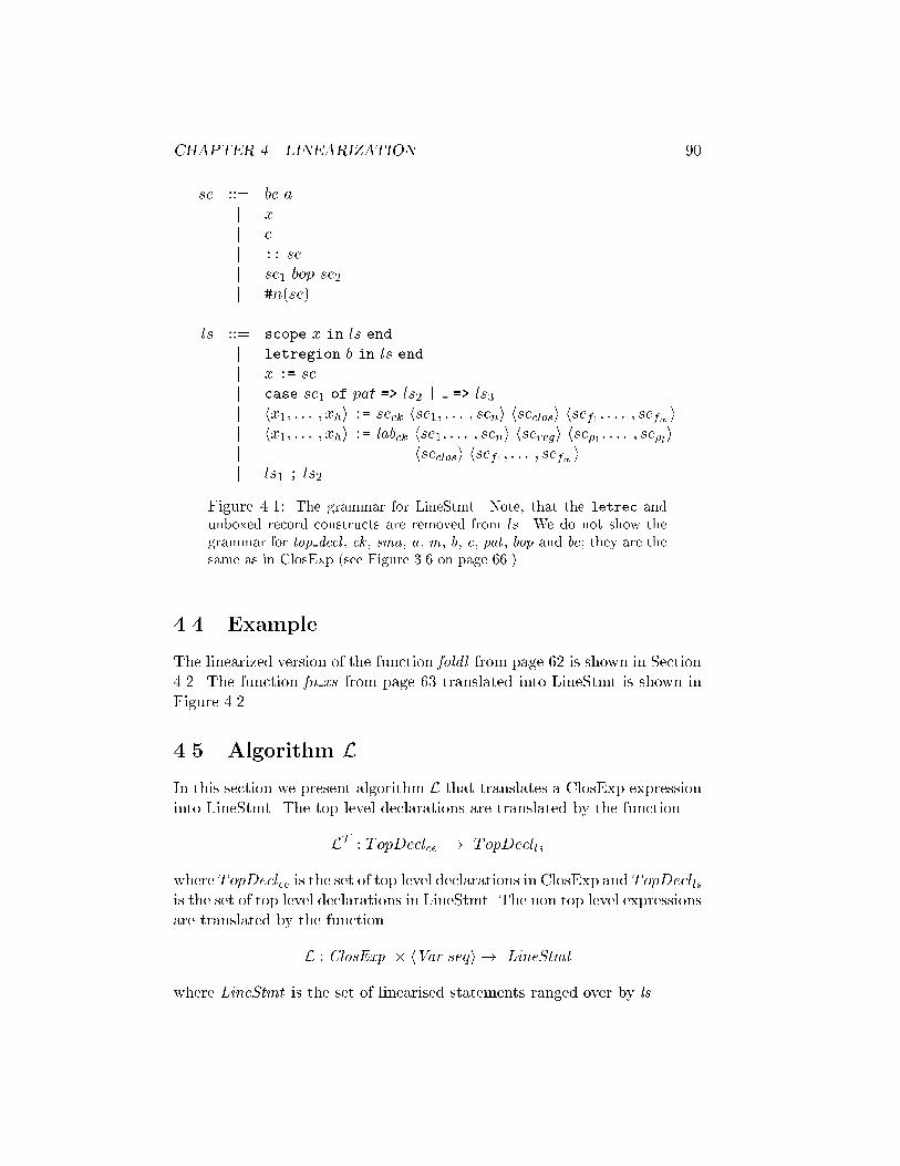
CHAPTER 4. LINEARIZATION 90
se ::= be a
j x
j c
j :: se
j se
1
bop se
2
j #n(se)
ls ::= scope x in ls end
j letregion b in ls end
j x := se
j case se
1
of pat => ls
2
| => ls
3
j hx
1
; : : : ; x
h
i := se
ck
hse
1
; : : : ; se
n
i hse
clos
i hse
f
1
; : : : ; se
f
m
i
j hx
1
; : : : ; x
h
i := lab
ck
hse
1
; : : : ; se
n
i hse
reg
i hse
�
1
; : : : ; se
�
l
i
j hse
clos
i hse
f
1
; : : : ; se
f
m
i
j ls
1
; ls
2
Figure 4.1: The grammar for LineStmt. Note, that the letrec and
unboxed record constructs are removed from ls. We do not show the
grammar for top decl , ck , sma , a , m, b, c, pat , bop and be ; they are the
same as in ClosExp (see Figure 3.6 on page 66.)
4.4 Example
The linearized version of the function foldl from page 62 is shown in Section
4.2. The function fn xs from page 63 translated into LineStmt is shown in
Figure 4.2.
4.5 Algorithm L
In this section we present algorithm L that translates a ClosExp expression
into LineStmt. The top level declarations are translated by the function
L
T
: TopDecl
ce
! TopDecl
ls
where TopDecl
ce
is the set of top level declarations in ClosExp and TopDecl
ls
is the set of top level declarations in LineStmt. The non top level expressions
are translated by the function
L : ClosExp � hVar seqi ! LineStmt
where LineStmt is the set of linearised statements ranged over by ls.

CHAPTER 4. LINEARIZATION 91
�
fn
fn xs
fargs=[xs], clos=c, res=[res ]g =>
scope v942 in
(case xs of
nil => res := #1(c)
| :: (v942 ) =>
scope x , xs' in
x := #0(v942 );
xs' := #1(v942 );
letregion r22 :4 in
scope k80 in
letregion r24 :4 in
scope k77 in
letregion r25 :2 in
scope rv , lv
1
, lv
2
in
rv := [atbot lf r24 , atbot lf r22 ] atbot lf r25;
lv
1
:= #2(c);
lv
2
:= #3(c);
hk77i := foldl
funcall
hlv
1
i hrvi hi hlv
2
i hi
end
end; (*r25*)
scope k79 in
scope lv
3
, k78, lv
4
in
lv
3
:= #2(c);
hk78i := (lv
3
)
fncall
hxi hlv
3
i hi;
lv
4
:= #1(c);
hk79i := k78
fncall
hlv
4
i hk78 i hi
end;
hk80i := k77
fncall
hk79 i hk77 i hi
end
end
end; (*r24*)
hresi := k80
fncall
hxs' i hk80 i hi
end
end (*r22*)
end)
end
Figure 4.2: The function foldl from page 63 translated into LineStmt.
Note variable lv
3
in the call to lv
3
that is used for both the code pointer
and function closure. The function lookup ve (page 74) will assign #2(c)
to two fresh lambda variables and not lv
3
only. However, the function
unify se then uni�es the two select expressions.

CHAPTER 4. LINEARIZATION 92
4.5.1 Top level declarations
We assume the number of values returned by each function to be known and
the function
RC : Label ! Int
returns the number of return values for each function represented with its
label.
L
T
[[�
fun
lab
cc => e]] =
let
val lv
i
= fresh lvar("lv i") i = 1; : : : ; RC(lab)
in
�
fun
lab
(cc + fres=[lv
1
; : : : ; lv
RC(lab)
]g) =>
L [[e]] hlv
1
; : : : ; lv
RC(lab)
i
end
The top level function �
fn
lab
cc => e is translated likewise. We write cc +
fres=[lv
1
; : : : ; lv
RC(lab)
]g as an abbreviation for constructing a new call con-
vention extended with the list of result variables. A sequence of top level
declarations is translated by:
L
T
[[top decl
1
;top decl
2
]] = L
T
[[top decl
1
]] ;L
T
[[top decl
2
]]
4.5.2 Simple Expressions
L [[c]] hlvi = lv := c
L [[x]] hlvi = lv := x
L [[be a]] hlvi = lv := be a
Boxed expressions are not changed in the translation.
L [[e
1
bop e
2
]] hlvi = lv := e
1
bop e
2
L [[#n(e)]] hlvi = lv := #n(e)
4.5.3 Expressions
L [[letrec f
lab
= be a in e end]] h
~
lvi =
scope f in
f := be a;
L [[e]] h
~
lvi
end

CHAPTER 4. LINEARIZATION 93
L [[e
ck
he
1
; : : : ; e
n
i he
clos
i he
f
1
; : : : ; e
f
m
i]] h
~
lvi =
h
~
lvi := e
ck
he
1
; : : : ; e
n
i he
clos
i he
f
1
; : : : ; e
f
m
i
L [[lab
ck
he
1
; : : : ; e
n
i he
reg
i he
�
1
; : : : ; e
�
l
i he
clos
i he
f
1
; : : : ; e
f
m
i]] h
~
lvi =
h
~
lvi := lab
ck
he
1
; : : : ; e
n
i he
reg
i he
�
1
; : : : ; e
�
l
i he
clos
i he
f
1
; : : : ; e
f
m
i
The lambda variables h
~
lvi are now explicitly marked as the return conven-
tion.
L [[letregion b in e end]] h
~
lvi =
letregion b in L [[e]] h
~
lvi end
L [[let val hx
1
; : : : ; x
n
i = e
1
in e
2
end]] h
~
lvi =
scope x
1
; : : : ; x
n
in
L [[e
1
]] hx
1
; : : : ; x
n
i;
L [[e
2
]] h
~
lvi
end
L [[he
1
; : : : ; e
n
i]] hlv
1
; : : : ; lv
n
i =
lv
1
:= e
1
;
.
.
.
lv
n�1
:= e
n�1
;
lv
n
:= e
n
L [[case e
1
of c => e
2
| => e
3
]] h
~
lvi =
case e
1
of
c => L [[e
2
]] h
~
lvi
| => L [[e
3
]] h
~
lvi
L [[case e
1
of ::(v) => e
2
| => e
3
]] h
~
lvi =
scope v in
case e
1
of
::(v) => L [[e
2
]] h
~
lvi
| => L [[e
3
]] h
~
lvi
end
We have two rules for the case construct because the pattern ::(v)
implicitly declares v and we therefore need a scope for v. We insert the
scope outside the case which is �ne in our grammar because we at most
can have one declaration. However, it does not work in the general case.
Consider the code

CHAPTER 4. LINEARIZATION 94
case e
1
of
::(v) => e
2
| ::'(hv
1
; v
2
i) => e
3
| => e
4
where we have two constructors :: and ::'. If the variables v; v
1
and v
2
are
spilled then variable v can share stack space with the variables v
1
and v
2
,
that is, v and v
1
; v
2
are not live at the same time. Introducing the scope
construct outside the case makes this sharing impossible with the o�set
calculation algorithm used in Chapter 7. However, it is not a problem in the
ML Kit because the case construct can only match constants so no variable
is ever declared in a pattern in a case construct.

Chapter 5
Register Allocation
The phases preceding register allocation assume an in�nite number of ma-
chine registers (i.e., variables). The closure conversion phase, for instance,
introduces a new variable whenever a value is selected from a closure with no
concern to how the value is stored at runtime (i.e., in a machine register or
in a memory cell). The target computer assumes all values to either reside
in machine registers or in memory.
The purpose of register allocation is to map the variables into machine
registers, memory locations or both. On most computers, and especially
RISC based computers, accessing values in memory is much more expensive
than accessing values in registers. It is essential for the running time of the
target program to map as many variables to machine registers as possible.
It is not possible to always map all variables to registers and some variables
must be stored in memory. We say such variables are spilled. Neither, is
it possible to always obtain an optimal mapping from variables to registers
and most algorithms are driven by heuristics directing the way registers are
chosen for variables (and likewise how variables are chosed to be spilled).
A popular register allocation method is graph coloring [13]. An interfer-
ence graph is built with nodes representing values (i.e., variables) and edges
representing interferences. Two nodes that interfere may not be assigned
the same register. There can be several reasons for two variables to inter-
fere but the usual reason is that they are live at the same time. Given the
interference graph and a set of colors we compute a coloring of the graph,
that is, we assign colors to the nodes and no two nodes connected with an
edge may be assigned the same color. The set of colors represent the set of
machine registers.
Register allocation can either be done locally on each function (or ba-
sic block) called intra{procedural register allocation or globally on entire
modules (or programs) called inter{procedural register allocation.
1
1
We use the term global for modules containing one or more functions. In many books
on optimizing compilers the term global refers to function wide optimizations and local
95

CHAPTER 5. REGISTER ALLOCATION 96
An intra{procedural register allocator does not have information about
register usage outside the function currently considered. It is therefore nec-
essary that all local values are at �xed places (often memory) when control
is transferred from one function to another. An inter{procedural register
allocator may use information about several functions in the program and
may therefore obtain better register mappings. For instance, it may be the
case that at every call to a function f then a large set of registers do not
contain live data and may therefore be used freely inside the function f ; or
if f only uses a few registers then the caller can use the other registers freely
even though f is called within the live range of the values in the registers.
A disadvantage with inter{procedural register allocators is that they often
depend on control ow information which is di�cult to obtain accurately in
a language with unknown functions [12, 38].
The graph color algorithm has two major problems. It may be computa-
tionally hard to color the interference graph and a variable is either assigned
a register or memory location for its entire life time. It may be better to
assign a variable a register in one part of a function and a memory location
in another part of the function. This may be done by range splitting (i.e.,
to use two variables for the same value with no overlapping life range) but
this is not included in the graph color algorithm.
It is widely believed that graph coloring is a wise choise for register allo-
cation. The average computation necessary for coloring can be made accept-
able and generating variables with short life ranges solves the range splitting
problem. For instance, the variables introduced by function insert se in the
closure conversion algorithm (Chapter 3) have small live ranges.
Other register allocation algorithms not based on graph coloring exists.
They are often motivated by the need to solve the register allocation problem
faster than is possible with graph coloring. For instance, an inter{procedural
register allocator based on graph coloring may build a huge interference
graph that is too costly to solve. Also, dynamic optimizations done at load
time require the optimizations to be almost linear which is not the case with
graph coloring.
A fast algorithm called linear scan uses the same liveness information
as graph coloring but instead of building an interference graph it is used to
compute a lifetime interval for each variable. A lifetime interval includes
the code that starts at the program point where the variable is �rst de�ned
and ends at the program point where it is last used. The lifetime intervals
can be sorted according to the order of the code. A �nite number of lifetime
intervals are active at each program point and they all compete for a register.
If there are more active lifetime intervals than registers then one or more
variables, represented by the active lifetime intervals, are spilled.
A recent study of a well written linear scan based algorithm and a well
to optimizations on basic blocks only [1, 37].

CHAPTER 5. REGISTER ALLOCATION 97
written graph color based algorithm has shown that in general the linear scan
approach is close to the quality of graph coloring [54]. However, the com-
pile time diverges as the programs get larger with more competing register
candidates, (i.e., more variables); on a program with 245 register candidates
graph coloring used 0.4 seconds and linear scan 1.5 seconds. On a program
with 6697 register candidates graph coloring used 15.8 seconds and linear
scan 4.5 seconds.
Many phases in the compiler introduce statements that move values from
one variable v
1
to another variable v
2
. If v
1
and v
2
are assigned the same
register then the move statement can be eliminated. We can traverse the
program after register allocation and remove unnecessary move statements.
However, we can do better. If there is no interference between the two
variables v
1
and v
2
then we can assign the same register to the variables and
thereby eliminate the move statement. This is called coalescing.
Our register allocator is intra{procedural and we believe graph coloring
is the best choice because the interference graphs are no larger than they
can be solved in acceptable time. The study discussed above has shown that
the result is in general slightly better than a linear scan based algorithm.
We use a variant of graph coloring with coalescing [6].
We try to merge two nodes in the interference graph if they are source
and destination of a move statement and does not interfere. We merge
the nodes only if we can prove that it is not harder to color the resulting
interference graph, that is, if we have a K color{able interference graph then
the resulting graph, with the two nodes merged, must still be K color{able.
The algorithm described in this chapter is based on the one given by Appel
[6, Chapter 11].
We �rst discuss the additions necessary to the intermediate language to
express register allocation information. We then discuss call conventions
(with caller and callee save registers), liveness analysis and explain the gen-
eral principles used in the graph color algorithm; especially how moves are
eliminated and how registers are chosen for variables. We do not discuss the
algorithm in detail because it is explained elsewere [6].
5.1 Revised Grammar
A few additions are necessary to the grammar for LineStmt in order to in-
clude register allocation information. Normally, a register allocator returns
a rewritten program where all variables have been replaced by machine reg-
isters. However, we do not remove lambda and region variables because they
are needed in the succeeding phases. Instead we insert register allocation
information into the code such that the code generator knows which regis-
ters the variables are mapped to. We keep the variables because we need
the scope information (scope and letregion constructs) in the phase that

CHAPTER 5. REGISTER ALLOCATION 98
calculates stack o�sets, Chapter 7.
One could annotate the register allocation information in two ways giving
a di�erent level of exibility.
1. For each scope lv in e end construct we can annotate the machine
register to which the lv is mapped as follows:
scope lv : phreg in e end
This says that lv has been mapped into the machine register phreg in
e.
2. We can also keep the scope construct as is, and then use a new con-
struct
e ::= regalloc lv 7! phreg
that tells the code generator that variable lv has been assigned ma-
chine register phreg. The assignment is valid until the next regalloc
construct reassigns lv to anoter machine register or cancels the assign-
ment:
e ::= regalloc lv 7! none
This implicitly says that from now on lv is spilled, (i.e., none is not a
valid color).
The �rst method is adequate for a graph color based register allocator work-
ing on entire function bodies as one entity because then any variable will
be mapped to the same register during the entire function. The second
method gives more exibility because a variable may be mapped to di�erent
machine registers during its life time. However, the extra exibility either
requires a more exible register allocator than graph coloring or a graph
color algorithm that considers the code between two function calls as one
entity instead of the entire function.
It is hard to see which is the best solution. We let the graph color
algorithm work on an entire function body as one entity because it seems
simpler. We then gain exibility by splitting registers in caller and callee
save registers which makes it possible to have registers live across function
calls. This is di�cult to achieve with a graph color algorithm working only
on the code between function calls. We annotate the register allocation
information on the scope constructs because it seems simpler and works
with our graph color method.
5.1.1 Store Type
When calculating stack o�sets we assign o�sets to spilled variables only.
The register allocator therefore annotate a store type (sty) on the scope

CHAPTER 5. REGISTER ALLOCATION 99
construct.
sty ::= stack
j phreg
where phreg 2 PhReg is a machine register. A phreg annotation says that the
variable is never spilled and stack means that there exists a path through
the function where the variable is spilled.
2
e ::= scope x : sty in e end
The variables in a call convention are replaced by a call convention store
type:
cc sty ::= LamVar : stack
j phreg
where lv :stack means that the parameter lv is passed in the call convention
on the stack and phreg says that the parameter (that was denoted by a
variable v before register allocation) is passed in the machine register phreg.
The variable v is removed from the call convention for reasons discussed in
the next section. A call convention is then as follows:
cc = fclos: cc sty option,
free: cc sty list,
args: cc sty list,
reg vec: cc sty option,
reg args: cc sty list,
res: cc sty list g
where for instance, args:cc sty list is a list of call convention store types
each denoting an argument parameter. At this point it is important to note
that a variable denoting a parameter passed on the stack has been declared,
(i.e., a stack slot has been reserved for the variable). A parameter passed
in a machine register is not bound to a variable (i.e., the variable has been
removed from the call convention). However, it may be the case that the
machine register needs to be spilled and this requires a slot on the stack to
be reserved. A stack slot is reserved by explicitly introducing the removed
variable (with scope) in the body of the function and bind it to the machine
register that it was replaced with. This is explained in the next section. We
let CC
sty
denote the set of call conventions with store types inserted ranged
over by cc
sty
.
It is not necessary to annotate store types on region variables at the
letregion construct because they always denote a known slot in the acti-
vation record of the function in which they are declared. This holds for both
�nite and in�nite regions.
2
Because we are compiling Standard ML where variables are immutable and a variable
keeps the same stack place while it is live then we store a variable only once in memory.

CHAPTER 5. REGISTER ALLOCATION 100
5.1.2 Call Conventions
Before building the interference graph we make dedicated machine registers
explicit in the program (e.g., machine registers used for argument and result
values at application points). This is necessary for the precolored variables,
that is, variables that are dictated a speci�c register by the call conventions.
Parameters and results passed on the stack do not need explicit scope
declarations in the body of the called function because they are already
stored on the stack. Actually we simplify matters even further by not letting
spilled parameters and results be part of the register allocator (i.e., if a
parameter is spilled by a call convention then it remains spilled after register
allocation). The simpli�cation is justi�ed by the fact that we reserve many
machine registers for arguments and results and if the number of arguments
or results exceeds the number of available machine registers then the register
pressure is high and we believe the advantage of letting them be register
allocated is limited.
3
Parameters and results passed in machine registers may be spilled during
register allocation. Say that a function takes variable v as argument and
the argument is passed in a machine register ph. Then v is removed from
the call convention and declared in the body of the function with a scope
construct. At entry to the function we assign v the value of ph. It is then
possible for the register allocator to spill the argument variable v and load
ph with another value. It is also possible that v is assigned another machine
register in which case the move statement becomes a copy between two
registers. It may also be the case that v and ph are coalesced in which case
the assignment is removed. It all depends on the register pressure in the
body of the function.
There are two main reasons for moving v out of the call convention
and into the body of the function: if v is spilled then the scope construct
automatically reserves a slot in the activation record by the calculate o�set
phase (Chapter 7) and the variable v is only declared once. It would be
confusing to have the same variable present in both the call convention and
in a scope construct because where is the variable then declared? It is not
declared in the call convention because the parameter is passed in a register!
Assuming we have two machine registers for passing arguments (phreg
1
and phreg
2
) and one for the result (phreg
1
) then the slightly modi�ed function
foldl from page 89 may be rewritten as the function below. We have added
another result variable res
2
that is returned on the stack to illustrate passing
both arguments and results in registers and on the stack.
�
fun
foldl
fargs=[phreg
1
], recvec=phreg
2
, clos=c:stack,
res=[phreg
1
,res
2
:stack]g =>
3
The number of available registers depends on the target architecture which may either
be a RISC or CISC machine.

CHAPTER 5. REGISTER ALLOCATION 101
scope res
1
in
scope f , rv in
f := phreg
1
;
rv := phreg
2
;
scope lv
1
, lv
2
, fn b in
lv
1
:= #1(rv );
lv
2
:= #0(rv );
hfn
b
i := �
fn b
[f , lv
1
, c] attop lv
2
;
res
1
:= fn b;
res
2
:= fn b
end
end;
phreg
1
:= res
1
end
5.1.3 Resolving Call Conventions
Given a call convention as de�ned on page 57 with variables donoting argu-
ment and result parameters we must convert it into a call convention that
speci�es how the parameters are passed, that is, either on the stack on in
registers.
The function
resolve cc : CC !
precolored arguments
z }| {
(LamVar � PhReg)list �
precolored results
z }| {
(LamVar � PhReg)list �CC
sty
makes this conversion and returns a list of precolored argument variables,
precolored result variables and a call convention with store type annotations
inserted. The compiler supports only one call convention, the standard call
convention, but any number of call conventions are easily supported. In case
more than one call convention is used, then an analysis deducing the call
conventions must be implemented. All functions which can be called at the
same application point must have the same call convention.
Assume, we have a list of machine registers for arguments args phreg
and a list of machine registers for results res phreg. We then assign the
variables in a call convention argument and result registers as follows. Re-
sult variables are assigned machine registers in the order left to right. If
res=[lvr
1
; : : : ; lvr
n
] and we have m = jres phregj � n then the �rst m vari-
ables (lvr
1
; : : : ; lvr
m
) in res are assigned a register from res phreg.
Argument parameters are resolved with the following order (priority):
clos, reg vec, args, free, reg args. For each entry, the variables are assigned
registers from args phreg.
For example, with args phreg = [q
1
; : : : ; q
9
], res phreg = [p
1
; p
2
] and call
convention

CHAPTER 5. REGISTER ALLOCATION 102
cc = fclos = c,
free = [f
1
; f
2
],
args = [a
1
; : : : ; a
9
],
reg vec = rv,
reg args = [],
res = [r
1
; : : : ; r
4
]g
then resolve cc(cc) returns
([(c; q
1
); (rv; q
2
); (a
1
; q
3
); : : : ; (a
7
; q
9
)],
[(r
1
; p
1
); (r
2
; p
2
)],
fclos = q
1
,
free = [f
1
: stack; f
2
: stack],
args = [q
3
; : : : ; q
9
; a
8
: stack; a
9
: stack],
reg vec = q
2
:,
reg args = [],
res = [p
1
; p
2
; r
3
: stack; r
4
: stack]g)
The arguments a
8
, a
9
, f
1
, f
2
and results r
3
, r
4
are passed on the stack
and the other variables are removed from the call convention and returned
as either precolored argument or precolored result variables. For instance,
result variable r
1
is precolored as register p
1
.
5.1.4 Rewriting LineStmt
As discussed above we must declare the precolored variables with scope
constructs such that a stack slot can be reserved in the case they are spilled.
We must also make sure that arguments and results, at application points,
are passed in either registers or on the stack speci�ed by the call convention.
In this section we show how to rewrite the body of a function such that this is
explicit. We believe it is better to have such information explicit in the term
because it makes it easier to implement the register allocation algorithm
and see what happens, (e.g., why is an argument variable coalesced with
register ph
1
and not ph
2
). The extra statements inserted does not e�ect the
resulting program because if they were not inserted then we would have to
incorporate the same information into the register allocation algorithm and
the algorithm would be harder to comprehend. We hope, that most of the
extra moves are removed by coalescing.
Given the function resolve cc we can rewrite a LineStmt program to
be on the same form as foldl on page 100.
We use the three functions:
resolve args : (LamVar � PhReg) list ! LineStmt
resolve res : (LamVar � PhReg) list ! LineStmt
resolve app : LineStmt! LineStmt

CHAPTER 5. REGISTER ALLOCATION 103
Declaring Argument and Result Variables
The function resolve args translates all argument variables passed in ma-
chine registers into a sequence of assignments. If resolve cc is called with
precolored argument variables: [(a
1
; r
1
); : : : ; (a
n
; r
n
)] then the sequence
a
1
:= r
1
;
.
.
.
a
n
:= r
n
is returned. The function resolve res does the opposite. Given the pre-
colored result variables [(a
1
; r
1
); : : : ; (a
n
; r
n
)] as argument the sequence of
assignments returned is
r
1
:= a
1
;
.
.
.
r
n
:= a
n
Application Points
The function resolve app resolves an application using a variant of re-
solve cc (called resolve app cc) working on call conventions containing
simple expressions and not variables only. The argument brackets are con-
verted into a temporary call convention and a list of argument and result
expressions passed in machine registers are returned from resolve app cc.
4
A sequence of copies between expressions and machine registers are then in-
serted around the application. Consider the application
hx
1
; : : : ; x
n
i := se
1
hse
2
; : : : ; se
m
i hse
1
i hi
The application is converted into the term
arg
1
:= se
1
;
.
.
.
arg
k
:= se
k
;
hres
1
; : : : ; res
h
; x
h+1
; : : : ; x
n
i :=
arg
1
harg
2
; : : : ; arg
k
; se
k+1
; : : : ; se
m
i harg
1
i hi;
x
1
:= res
1
;
.
.
.
x
h�1
:= res
h�1
;
x
h
:= res
h
4
The function resolve app cc is identical to resolve cc except that resolve app cc
has simple expressions in each entry of the call convention and not variables.

CHAPTER 5. REGISTER ALLOCATION 104
where arg
i
and res
j
are machine registers. Argument and result values not
assigned machine registers by the standard call convention are passed on the
stack (e.g., se
k+1
; : : : ; se
m
and x
h+1
; : : : ; x
n
). Notice that the translation
preserves the property that machine registers are never live across an ap-
plication. This property is used in the phase that inserts ush statements,
Chapter 6. Note, that we never insert assignments after a tail call; the
assignments are never executed.
Translation
The LineStmt program is translated with the function
CC
T
: TopDecl
ls
! TopDecl
ls
working on top level declarations and the body of each function is translated
by
CC : LineStmt ! LineStmt
Below we show the interesting cases:
CC
T
[[�
fun
lab
cc => ls]] =
let
val (args, res, cc
sty
) = resolve cc(cc)
in
�
fun
lab
cc
sty
=>
scope to lvar seq(res) in
scope to lvar seq(args) in
resolve args(args);
CC [[ls]]
end;
resolve res(res)
end
end
The function to lvar seq transforms a list [(a
1
; r
1
); : : : ; (a
n
; r
n
)] into the
sequence a
1
; : : : ; a
n
(i.e., we declare the lambda variables that are mapped
into machine registers).
CC [[ls
1
;ls
2
]] = CC [[ls
1
]] ; CC [[ls
2
]]
We do a forward scan of the program.
CC [[hx
1
; : : : ; x
n
i := se
1
hse
2
; : : : ; se
m
i hse
1
i hi]] =
resolve app(hx
1
; : : : ; x
n
i := se
1
hse
2
; : : : ; se
m
i hse
1
i hi)

CHAPTER 5. REGISTER ALLOCATION 105
�
fn
fn xs
fargs=[ph
2
], clos=ph
1
, res=[ph
1
]g =>
scope res in
scope xs , c in
c := ph
1
;
xs := ph
2
;
scope v942 in
(case xs of
nil => res := #1(c)
|:: (v942 ) =>
scope x , xs' in
x := #0(v942 );
xs' := #1(v942 );
letregion r22 :4 in
scope k80 in
letregion r24 :4 in
scope k77 in
letregion r25 :2 in
scope rv , lv
1
, lv
2
in
rv := [atbot lf r24 , atbot lf r22 ] atbot lf r25;
lv
1
:= #2(c);
lv
2
:= #3(c);
ph
1
:= lv
2
;
ph
2
:= rv;
hph
1
i := foldl
funcall
hlv
1
i hph
2
i hi hph
1
i hi;
k77 := ph
1
end
end; (*r25*) end
Figure 5.1: Part one of the function fn xs with the precolored
variables made explicit and application points resolved. We have
args phreg=[ph
1
; ph
2
] and res phreg=[ph
1
]. No arguments or results are
passed on the stack.

CHAPTER 5. REGISTER ALLOCATION 106
scope k79 in
scope lv
3
, k78, lv
4
in
lv
3
:= #2(c);
ph
1
:= lv
3
;
ph
2
:= x;
hph
1
i := (lv
3
)
fncall
hph
2
i hph
1
i hi;
k78 := ph
1
;
lv
4
:= #1(c);
ph
1
:= k78;
ph
2
:= lv
4
;
hph
1
i := k78
fncall
hph
2
i hph
1
i hi;
k79 := ph
1
end;
ph
1
:= k77;
ph
2
:= k79;
hph1i := k77
fncall
hph
2
i hph
1
i hi;
k80 := ph
1
end
end
end; (*r24*)
ph
1
:= k80;
ph
2
:= xs
0
;
hph1i := k80
fncall
hph
2
i hph
1
i hi;
res := ph
1
end
end (*r22*)
end)
end
end;
ph
1
:= res
end
Figure 5.2: Part two of the function fn xs with the precolored variables
made explicit and application points resolved.

CHAPTER 5. REGISTER ALLOCATION 107
A letrec application is done similarly.
With the LineStmt program in this form we can build the interference
graph. Figure 5.1 and 5.2 shows the example function fn xs from Figure 4.2
on page 91 with precolored variables made explicit.
Precolored registers do not spill so their live range must be small. This
is indeed the case in foldl where the argument registers are stored in argu-
ment variables at entry to the function and result registers are given their
value at exit from the function. The live ranges are also minimized around
applications.
5.2 Dummy Register Allocator
A nice e�ect of having call conventions explicit in the LineStmt code is that
we can compile the program without using a register allocator or at least
use a trivial register allocator only. Our trivial register allocator spills all
variables, that is, annotate all scope introduced variables with stack. The
code generator then inserts load and store code such that only temporary
registers are used besides the registers used in the call convention.
We found it invaluable to use such a simple register allocator in the
early stages of the compiler because we did not have a complicated reg-
ister allocator algorithm to debug while debugging the mandatory phases
of the backend. Also, the garbage collector was easier to debug without a
complicated register allocator.
5.3 Liveness Analysis
To build the interference graph we need a liveness analysis that, for each
program point, computes the set of live variables, that is, the variables that
contain a value that is needed for the remainder of the computation.
For imperative languages the liveness analysis is normally based on a
control ow graph that, for each statement, has an edge to the statements
that may follow. If the program contains loops, then the control ow graph
contains cycles. Liveness is found by a �xed point computation on the con-
trol ow graph. We compute liveness information locally for each function
and because loops are implemented with function calls in Standard ML then
we do not have loops locally in each function. We can then compute the
liveness information by a single backward scan of the LineStmt program.
Consider the LineStmt code
scope x; y; z in
x := 0 (1)
y := x + 42 (2)
z := x + y (3)

CHAPTER 5. REGISTER ALLOCATION 108
x := 42 (4)
z := z + x (5)
.
.
.
end
The liveness information is computed using def and use sets of each state-
ment, that is, the set of variables that are de�ned and used respectively
when the statement is evaluated. Note that the same variable can be used
and de�ned in the same statement (e.g., z := z + x). We let the functions
def and use return the set of de�ned and used variables for the statement
given as argument. For assignment and addition we have:
def(v
1
:= v
2
+ v
3
) = fv
1
g
use(v
1
:= v
2
+ v
3
) = fv
2
, v
3
g
The def and use functions for LineStmt are de�ned in Section 5.3.1.
The live range of a variable is the code between the �rst de�nition and
last use of the variable. The same variable may be de�ned at di�erent
program points in imperative languages but a variable is de�ned only once
in Standard ML. LineStmt is not a functional language but because it is a
linearized version of a functional language then we have a similar property,
that is, a variable is initialized only once during program evaluation, see
Section 4.1 on page 86. This is a unique property because then a variable
needs to be stored in memory at most one time even though it is spilled.
The live ranges for x, y and z in the example program above are
z = f4 7! 5, 3 7! 4g
x = f4 7! 5, 2 7! 3, 1 7! 2g
y = f2 7! 3g
Note that the above program cannot be a linearized version of a ClosExp
program because x is de�ned twice. The set of live variables at each state-
ment is computed by looking at each statement in reverse order. For each
statement we maintain a set live that is the set of live variables at entry to
the statement. If we assume z to be live after statement 5 (i.e., live(6)=fzg),
then we have
live(5) = use(5) [ (live(6) n def(5)) = fz; xg [ (fzg n fzg) = fz; xg
live(4) = use(4) [ (live(5) n def(4)) = fg [ (fz; xg n fxg) = fzg
and in general
live(i) = use(i) [ (live(i+ 1) n def(i))

CHAPTER 5. REGISTER ALLOCATION 109
5.3.1 Def and Use Sets for LineStmt
The functions def and use for LineStmt constructs are easily de�ned. The
table below shows the def and use sets for various simple constructs:
Construct def use
sma lv fg flvg
sma � fg fg
� : m fg fg
c fg fg
::x fxg fg
An allocation point sma � does not de�ne � because � is a constant at
runtime (i.e., an o�set from the stack pointer found at compile time). The
pattern ::x de�nes the variable x.
Boxed expressions do not de�ne variables. The use sets are calculated
as follows:
use((se
1
; : : : ; se
n
)) =
S
i=1;::: ;n
use(se
i
)
use(�
lab
[se
f
1
; : : : ; se
f
n
]) =
S
i=1;::: ;n
use(se
f
i
)
use([a
1
; : : : ; a
n
]
regvec
) =
S
i=1;::: ;n
use(a
i
)
use([se
f
1
; : : : ; se
f
n
]
sclos
) =
S
i=1;::: ;n
use(se
f
i
)
Def and use sets for simple expressions are found below:
Construct def use
be a fg use(be) [ use(a)
x fg fxg
c fg fg
:: se fg use(se)
se
1
bop se
2
fg use(se
1
) [ use(se
2
)
#n(se) fg use(se)
5.4 Interference Graph
With liveness information we can compute the interference graph ig where
nodes denote variables and we have an edge between two nodes if they
interfere. Two variables v
1
and v
2
may interfere for several reasons but
the usual situation is that v
1
and v
2
are live at the same time (i.e., they
cannot be assigned the same register). Other interferences may come from
instruction sets where some instructions can access a limited number of the
registers only. Then the variables in the instruction interfere with all the
registers that the instruction does not access. We only consider interferences
of the �rst kind so two variables interfere i� there exists a program point
where they are both live.
We let IG be the set of interference graphs ranged over by ig.

CHAPTER 5. REGISTER ALLOCATION 110
5.4.1 Unnecessary Copy Related Interferences
We give the assignment construct special treatment. A copy x := y does
not make x and y interfere because they contain the same value and may
therefore be assigned the same register. If, however, one of the registers, say
x, is rede�ned while y is still live then an interference edge will be inserted.
5
This is indeed necessary because at that time they do not necessarily contain
the same value.
Edges are added to an interference graph ig using, for each statement
ls, the two rules
1. if ls is a copy d := s, and the live set (live out) is flv
1
; : : : ; lv
n
g then
we add edges (d,lv
i
) to ig for all lv
i
not equal to s.
2. if ls is not a copy, de�nes variable d and the live set (live out) is
flv
1
; : : : ; lv
n
g, then we add the edges (d; lv
1
); : : : ; (d; lv
n
) to ig.
The graph ig is undirected.
5.4.2 Move Related Nodes
For every copy d := s we insert a move related edge in ig. A move related
edge is not an interference edge. Move related edges makes it possible to
distinguish move related nodes (i.e., d and s) from non move related nodes.
In the examples to come we use dotted edges for move related edges and
normal edges for interference edges. A node can be categorized as either:
1. a move related node (i.e., the node has at least one move related edge
and maybe other interference edges).
2. a non move related node (i.e., the node does not have any move related
edges).
3. a constrained move related node (i.e., a node with a move related
edge to a node n and an interference edge also to node n). Then it
is impossible to coalesce the two nodes. We remove all move related
edges from constrained move related nodes.
5.4.3 Building IG
With the def and use functions de�ned in Section 5.3.1 we can state the
algorithm that computes the interference graph.
IG
T
: TopDecl
ls
! IG
5
This never happens because we are compiling Standard ML and not an imperative
language.

CHAPTER 5. REGISTER ALLOCATION 111
works on top level declarations. The body of a function is handled by
IG : LineStmt �P(LamVar)� IG! P(LamVar)� IG
where P(LamVar) is ranged over by live and is the set of live variables.
Top Level Functions
IG
T
[[�
fun
lab
cc => ls]] =
let
val (live; ig) = IG [[ls]] fg fg
in
ig
end
The empty graph is written fg.
Statements
We do a backward scan on the statements and collect liveness information
at the same time that we insert either interference or move related edges
into ig.
IG [[scope x in ls end]] live ig = IG [[ls]] live ig
IG [[letregion b in ls end]] live ig = IG [[ls]] live ig
IG [[lv
1
:= lv
2
]] live ig =
(flv
2
g [ (live n flv
1
g),
addMoveEdge(addEdge(ig; flv
1
g; live n flv
2
g); lv
1
; lv
2
))
IG [[lv := (se
1
; : : : ; se
n
) a]] live ig
((live n flvg) [ use((se
1
; : : : ; se
n
) a),
addEdge(ig; flvg; live [ use((se
1
; : : : ; se
n
) a)))
IG [[lv := se]] live ig =
((live n flvg) [ use(se), addEdge(ig; flvg; live))
IG [[case se
1
of pat => ls
2
| => ls
3
]] live ig =
let
val (live
2
; ig
2
) = IG [[ls
2
]] live ig
val (live
3
; ig
3
) = IG [[ls
3
]] live ig
2
val live
1
= live
2
[ live
3
in
(use(se
1
) [ (live
1
n def(pat)), addEdge(ig
3
,def(pat),live))
end
IG [[hx
1
; : : : ; x
n
i := se
ffncall;funcallg
hse
1
; : : : ; se
n
i hse
clos
i hse
f
1
; : : : ; se
f
m
i]] live ig =
((
S
i2fck;1;::: ;n;clos;f
1
;::: ;f
m
g
use(se
i
)) [ (live n fx
1
; : : : ; x
n
g),
addEdge(ig; fx
1
; : : : ; x
n
g; live [ fx
1
; : : : ; x
n
g))
IG [[hx
1
; : : : ; x
n
i := se
ffnjmp;funjmpg
hse
1
; : : : ; se
n
i hse
clos
i hse
f
1
; : : : ; se
f
m
i]] live ig =

CHAPTER 5. REGISTER ALLOCATION 112
((
S
i2fck;1;::: ;n;clos;f
1
;::: ;f
m
g
use(se
i
))),
addEdge(ig; fx
1
; : : : ; x
n
g; fx
1
; : : : ; x
n
g))
IG [[ls
1
; ls
2
]] live ig =
let
val (live
2
; ig
2
) = IG [[ls
2
]] live ig
in
IG [[ls
1
]] live
2
ig
2
end
The rule for letrec application is similar to the rule for ordinary application.
Note that if more than one variable is de�ned as in an application then the
de�ned variables interfere with themselves and the live variables.
The function
addEdge : IG�P(LamVar)�P(LamVar)! IG
adds interference edges between variables in the two variable sets. The
function
addMoveEdge : IG� LamVar � LamVar ! IG
adds a move related edge between the two variables.
5.5 Spilling
Spilling a variable normally requires rewritting the program where a new
temporary will fetch the spilled variable and die right after the use. For
instance, if variable x is spilled we have
y = x + z ===x is spilled===> tmp = Fetch(x)
y = tmp + z
and tmp has a tiny life range. However, the rewritten program has to go
through the register allocation phase again (i.e., iterated register allocation).
In the ML Kit version 2 (and version 3) [22, 49, 50] we simpli�ed matters a
bit because we never rewrite the program if a variable is spilled. Instead we
reserve four registers that are not used by the register allocator.
The four registers are reserved for the purpose of compiling simple ex-
pressions and fetching spilled variables. For instance, the machine code to
allocate a region requires a few extra registers. Given any statement with
all variables spilled it is possible to compile it with the use of no more than
four registers.
The simpli�cation gives a less good register usage because the four re-
served registers are never used by the register allocator even though they
are not needed to compile all the statements. It may be solved by letting all
registers be available to the register allocator. If the code generator requires

CHAPTER 5. REGISTER ALLOCATION 113
additional registers to compile a statement then the requirements may be
build into the interference graph, that is, let the statements interfere with all
registers that are needed to compile the statements. This can be controlled
by the def and use functions. We do not use this method and still reserve
a number of registers for the code generator.
6
It is not necessary to insert spill code explicitly and use iterated regis-
ter allocation because we reserve temporaries for the code generator. This
speeds up the register allocator and we believe the performance degradation
to be moderate (i.e., the register allocator still has enough registers on a
RISC machine).
5.5.1 Statements Are Not Like Three Address Instructions
Register allocation is normally performed on three address like instructions
which are simpler than the statements in LineStmt. This means that we
perform register allocation on a term with less nodes than if we used three
address instructions which is good for the running time of the algorithm but
bad for the live ranges of variables containing intermediate values.
Consider the following assignment of a record expression where all vari-
ables x
1
; : : : ; x
n
are spilled.
x:=(x
1
; : : : ; x
n
)
If we have K machine registers and n > K then it is impossible to store
all variables in temporary registers. It is not possible to perform register
allocation on
scope tmp
1
; : : : ; tmp
n
in
tmp
1
:= x
1
;
.
.
.
tmp
n
:= x
n
;
x := (tmp
1
; : : : ; tmp
n
)
end
where all temporaries have to be machine registers. We reserve n registers
for a record with n elements which is an unreasonable amount. If we were
using three address code then an n element record would probably only
require two registers; one index register and one for the elements. This
is not possible in LineStmt because we must put all elements in registers
before allocating the record. However, this can be solved by using an alloc
primitive that can allocate memory for the record and an update primitive
to initialize each element:
6
The discussion assumes that the targe machine is a RISC machine. For CISC machines
with less registers it may not be necessary to reserve temporary registers because most
instructions can probably fetch from memory, perform the operation and then store the
result in memory again if necessary.

CHAPTER 5. REGISTER ALLOCATION 114
scope tmp
1
in
x := alloc(n);
tmp
1
:= x
1
;
update(x; 0; tmp
1
);
.
.
.
tmp
1
:= x
n
;
update(x; n� 1; tmp
n�1
);
end
We will probably use this technique in the future and thereby reduce the
register pressure.
5.6 Graph Coloring With Coalescing
After the interference graph ig is built the register allocator cycles though
the following phases that remove nodes from ig and pushes them on a stack.
Let K be the number of available machine registers (i.e., colors). The degree
of a node is the number of interference edges on the node. The move related
edges are not part of the degree.
Simplify: All non move related nodes of degree less than K are
removed from ig.
Coalesce: If simplify is not possible then do conservative coa-
lescing (see below) and return to simplify again.
Freeze: If neither simplify nor coalescing is possible, then choose
a move related node of low degree and remove the move re-
lated edges from that node. The node is not a move related
node anymore and may be removed by the simplify phase
which is applied next.
Spill: If we cannot simplify, coalesce or freeze a node then we
have to spill a variable. We calculate the priority (see be-
low) of the remaining nodes and remove the variable with
the lowest priority. We then try simplify again.
When all nodes are removed from ig we start popping nodes from the
stack. Each node is inserted in ig again and assigned a color that is not
assigned to any of the neighbors of the inserted node. We assign colors from
the caller save and callee save sets as described in Section 5.7 below. Spilled
variables are also inserted in ig and we try to assign a color even though
they were marked as potential spills on the stack. Sometimes it is possible
to assign a color to a variable that was considered spilled during the simplify
phase. For instance, if some of its neighbors share the same color or other
neighbors are spilled too. If it is not possible to color a potential spilled
variable we call it an actual spilled variable.

CHAPTER 5. REGISTER ALLOCATION 115
5.6.1 Conservative Coalescing
If an interference graph ig can be colored with M registers, then we call
it conservative coalescing when we can union two nodes in ig and still be
guaranteed that the resulting interference graph is M color{able. Appel
gives two strategies and proves that they are conservative [6, page 232]:
Briggs: Two nodes n
1
and n
2
can be coalesced if the resulting
node has fewer that K neighbors.
George: Two nodes n
1
and n
2
can be coalesced if for every
neighbor m to n
1
, either m has degree less than K or m is
also a neighbor to n
2
.
5.6.2 Spill Priority
To �nd an adequate node to spill we calculate a priority based on how many
times the variable is used in the program and the degree. Variables with a
large number of uses and low degree get a higher priority. Variables with
low priority are spilled.
priority(lv)=
uses(lv) + defs(lv)
degree(lv)
The functions uses and defs return the number of times the variable is used
and de�ned in the function.
5.6.3 Implementation
Appel gives an e�cient algorithm which can be adjusted to the speci�cs of
LineStmt and the ML Kit [6]. As noted in the introduction Elsman has
started the implementation in the ML Kit using the algorithm by Appel.
5.7 Caller and Callee Save Registers
If we have caller save registers only then it is necessary to save all live
registers before an application. If we have callee save registers only then the
called function must save all registers that it uses. Both methods may lead
to an excessive number of stores. Consider the code
f(: : : ) =
.
.
.
x := 5; g(x) = y := x + 1;
y := 6; a := y * 43;
z := y + x; b := a + y;
q := g(y); res := b

CHAPTER 5. REGISTER ALLOCATION 116
a := q + x;
b := q + z;
.
.
.
With caller save registers only, we have to ush the registers to which z
and x are bound at the application to g and fetch them afterwards. With
callee save registers only we have to ush the registers to which y, a and
b are bound in g and fetch them before we return the result res. With a
combination of callee and caller save registers we can allocate x and z to
callee save registers and avoid ushing them in f . In g we can bind y, a and
b to caller save registers because their live range do not cross an application.
Then we avoid ushing any variables at all.
Flushes across applications may be totally avoided by having the appli-
cation expression de�ne all caller save registers when the interference graph
is created. If a variable is not live across a function call then it will likely be
allocated to a caller save register. If a variable is live across the application
then it interferes with all caller save registers and will either be assigned a
callee save register or spilled. With caller save registers r
1
; r
2
and callee save
register r
3
a possible register assignment is: z : r
3
; x : spill; y : r
1
; q : r
1
; a : r
2
and b : r
1
. The variable x is spilled because we only have one callee save
register and it is given to z which is also live across the call to g. Both z
and x interfere with all caller save registers and hence one of them must be
spilled.
We can do better because we may bind x to a caller save register and
then store it across the function call. This is better than spilling where the
variable is held in memory all the time. This is achieved by not having the
call statement de�ne all caller save registers. Instead we mark variables with
a live range that crosses an application.
7
We then assign colors depending
on the marks. Variables not crossing applications are assigned caller save
registers if possible and variables crossing applications are assigned callee
save registers if possible. With this method a possible coloring is: y : r
1
; z :
r
3
; x : r
2
; q : r
1
; a : r
2
and b : r
1
. Now x is assigned a caller save register.
As an example of how registers can be divided into caller and callee
save registers we take a closer look at the HP PA-RISC architecture. The
HP PA-RISC machine has 32 general purpose registers [41, 40, 39].
8
The
Procedure Calling Convention manual [40] speci�es the callee save registers
to be gr
3
; : : : ; gr
18
and caller save registers to be gr
1
; gr
19
; : : : ; gr
26
; gr
28
and gr
29
. The convention is used by compilers supported by HP. We do not
have to use the same convention and it seems better to increase the number
7
This is done similarly to algorithm F in Chapter 6.
8
There are also oating point registers and they can also be divided into caller and
callee save registers but we limit the discussion to general purpose registers only.

CHAPTER 5. REGISTER ALLOCATION 117
Figure 5.3: All interferences in function fn xs.
of caller save registers. The reason is that all arguments and results must
be passed in caller save registers and we expect to get a high demand on
registers to be used in the call conventions.
We note that it may not be possible to be this generous with caller save
registers on other architectures like X86 based machines.
5.8 Example
Figure 5.3 shows all interferences in the example function fn xs from Figure
5.1 and 5.2. Figure 5.4 shows all non constrained move related nodes. We
assume K = 5 with ph1; ph2 and ph3 as caller save registers and ph4; ph5
as callee save registers.
We can simplify node v942 with only one interference edge and then
coalesce the nodes ph1 ,k80 ,lv2 ,res ,lv3 and k78 using coalescing strategy
George. For example, node ph1 interfere with the nodes ph2 , ph3 , k77 ,
k79 , ph4 , lv1 , rv , xs' , lv4 , ph5 , x and c. Node k80 interfere with the nodes

CHAPTER 5. REGISTER ALLOCATION 118
Figure 5.4: All move related nodes in function fn xs. We have removed
all constrained move related nodes.
ph2 and xs' . Because both nodes that interfere with k80 (i.e., ph2 and xs' )
interfere with ph1 then k80 and ph1 can be coalesced.
We can also coalesce the nodes ph2 ,k79 ,xs and rv using coalescing strat-
egy George. At �rst it seems that we cannot coalesce rv with ph2 because
lv2 does not interfere with ph2 . But after ph1 and lv2 are coalesced then
we can. The resulting graph is shown in Figure 5.5. There are no more
move related nodes.
We can then simplify lv4 with degree 3, see Figure 5.6. We do not have
more low degree moves and no more move related nodes. We therefore spill
a variable.
We calculate priorities for the 5 candidates
Variable Defs+Uses Degree Priority=
Defs+Uses
Degree
lv
1
2 5 0:40
k77 3 5 0:60
x 2 6 0:33
xs
0
2 6 0:33
c 6 6 1:00
The variable xs
0
, and x has lowest priority so we arbitrarily make xs
0
a
potential spill. Then we simplify lv1 with degree 4. The remaining variables
k77 , x and c can also be simpli�ed. We have spilled and simpli�ed in the
following order:
stack = [c; x; k77; lv1; xs
0
; lv4; v942]
with c on top of the stack. We have underlined the variables with a live range
crossing at least one application. We want to assign the underlined variables
callee save registers (i.e., ph
4
; ph
5
) and the non underlined variables caller
save registers (i.e., ph
1
; ph2 and ph3) whenever possible. We pop and assign

CHAPTER 5. REGISTER ALLOCATION 119
Figure 5.5: We have simpli�ed v942 and coalesced the nodes
ph1 ,k80 ,lv2 ,res and lv3 . We have also coalesced the nodes ph2 ,k79
and xs.
Figure 5.6: We have simpli�ed lv4 .

CHAPTER 5. REGISTER ALLOCATION 120
Figure 5.7: All nodes are now popped from the stack and inserted. We
have also removed the nodes ph
3
; ph
4
and ph
5
as they are only used by
the algorithm.
the following colors to the variables:
Variable Interfere With Assigned Color
c ph
1
; ph
2
ph
4
x ph
1
; ph
2
; ph
4
ph
5
k77 ph
1
; ph
2
; ph
4
; ph
5
ph
3
lv1 ph
1
; ph
2
; ph
4
; ph
5
ph
3
xs
0
ph
2
; ph
2
; ph
3
; ph
4
; ph
5
actual spill
lv4 ph
1
; ph
3
ph
2
v942 ph
5
ph
1
We do not have any callee save registers left for k77 so k77 is assigned the
caller save register ph
3
. The only variable that has to be ushed across
function calls is k77 and the two callee save registers at entry and exit of
the function. The resulting interference graph after inserting variables is
shown in Figure 5.7.
With the above register assignments and the coalesced nodes we have
rewritten the function fn xs to include register allocation information, see
Figure 5.8 and 5.9. It is important not to substitute registers for variables
yet because we need to compute the live range of each variable when we
insert fetch and ush instructions, see Chapter 6.

CHAPTER 5. REGISTER ALLOCATION 121
�
fn
fn xs
fargs=[ph
2
], clos=ph
1
, res=[ph
1
]g =>
scope res :ph
1
in
scope xs :ph
2
, c:ph
4
in
c := ph
1
;
xs := ph
2
;
scope v942 :ph
1
in
(case xs of
nil => res := #1(c)
|:: (v942 ) =>
scope x :ph
5
, xs
0
:stack in
x := #0(v942 );
xs' := #1(v942 );
letregion r22 :4 in
scope k80 :ph
1
in
letregion r24 :4 in
scope k77 :ph
3
in
letregion r25 :2 in
scope rv :ph
2
, lv
1
:ph
3
, lv
2
:ph
1
in
rv := [atbot lf r24 , atbot lf r22 ] atbot lf r25;
lv
1
:= #2(c);
lv
2
:= #3(c);
ph
1
:= lv
2
;
ph
2
:= rv;
hph
1
i := foldl
funcall
hlv
1
i hph
2
i hi hph
1
i hi;
k77 := ph
1
end
end; (*r25*) end
Figure 5.8: Part 1 of fn xs where we have inserted register allocation
information but not removed any assignments or simpli�ed it otherwise.
This is done by Substitution and Simplify, Chapter 8.

CHAPTER 5. REGISTER ALLOCATION 122
scope k79 :ph
2
in
scope lv
3
:ph
1
, k78:ph
1
, lv
4
:ph
2
in
lv
3
:= #2(c);
ph
1
:= lv
3
;
ph
2
:= x;
hph
1
i := (lv
3
)
fncall
hph
2
i hph
1
i hi;
k78 := ph
1
;
lv
4
:= #1(c);
ph
1
:= k78;
ph
2
:= lv
4
;
hph
1
i := k78
fncall
hph
2
i hph
1
i hi;
k79 := ph
1
end;
ph
1
:= k77;
ph
2
:= k79;
hph1i := k77
fncall
hph
2
i hph
1
i hi;
k80 := ph
1
end
end
end; (*r24*)
ph
1
:= k80;
ph
2
:= xs
0
;
hph1i := k80
fncall
hph
2
i hph
1
i hi;
res := ph
1
end
end (*r22*)
end)
end
end;
ph
1
:= res
end
Figure 5.9: Part 2 of fn xs where we have inserted register allocation
information but not removed any assignments or simpli�ed it otherwise.
This is done by Substition and Simplify, Chapter 8.

Chapter 6
Fetch And Flush
After register allocation (Chapter 5) we have mapped variables to either
machine registers or stack locations. If a variable is mapped to a caller save
register and the variable is live across a function call then it is necessary to
store its value before calling the function and retrieve its value after the call;
the caller save register may be overwritten in the called function. We do
not have to store variables mapped to callee save registers because they are
always preserved by the called function. In this chapter we present a few
phases that insert fetch and ush statements such that caller save registers
containing values live across an application are preserved.
The set of variables to ush are the variables that ful�lls all of the re-
quirements:
� the variable is locally bound (i.e., bound with a scope construct). In
contrast, argument and return values passed on the stack (i.e., vari-
ables with stack annotations in the call convention for the function)
are not said to be locally bound. Stack slots have been reserved for
such variables in the call convention before the function is entered.
� the variable has a live range that crosses an application, that is, the
variable is de�ned before the application and used after the applica-
tion.
� the variable has not already been ushed (i.e., we only ush variables
once in a function).
� the variable is assigned a caller save register. Variables assigned callee
save registers are ushed at entry to the function.
We ush callee save registers that are used within the function at entry
to the function (i.e., before the registers are assigned another value). We
fetch callee save registers at program points where control leaves the function
(i.e., at tail calls, raise and returns).
123

CHAPTER 6. FETCH AND FLUSH 124
A backward scan on the LineStmt program is used to compute the live
variables and then a forward transform inserts ush statements at selected
program points.
It is not obvious what program points should be chosen to ush and
fetch variables. H�jfeld et. al. discuss this in detail [38, Section 6.9]. We
simplify the discussion and consider two placement strategies only for ush
statements. We can ush a variable before the �rst application where the
variable is live or immediately after the statement that de�nes the variable.
Conditionals complicates the insertion of ush statements before applica-
tions because if one branch contains an application and another branch
does not, then ushing the variable in only one branch is not safe if the
variable is live across another application after the conditional. We choose
the simple solution and ush variables right after they are de�ned. If a
variable is de�ned in a conditional then all branches will contain a ush
statement because either a variable is not de�ned in a branch or it is de�ned
in all branches. This property is guaranteed by the linearization phase, see
Section 4.1. Only one ush statement is evaluated at runtime.
We insert a fetch v statement after a non tail call if variable v is bound
to a caller save register and used before the next call. We could also wait and
fetch v just before the use of v but then again conditionals may complicate
matters. Also, the register allocater has mapped v to a register for the entire
function so fetching earlier does not in uence the register pressure. Actually
fetching ealier may be good for the performance of the memory subsystem
but it is di�cult to verify such statements.
6.1 Revised Grammar
We extend LineStmt with the statements
ls ::= flush (LamVar [ PhReg)
j fetch (LamVar [ PhReg)
to ush and fetch a variable or a machine register. The register allocator
annotates a store type sty (Section 5.1.1) on each variable when it is de-
clared. We extend the storage type to include the case when a variable is
assigned a register that needs to be ushed.
sty ::= stack
j phreg
j flushed phreg
We ush a callee save register if the register is de�ned in the body of the
function. The question is then: where should we ush the register? Consider
the code fragment:

CHAPTER 6. FETCH AND FLUSH 125
scope v
1
:phreg
1
in
.
.
.
scope v
2
:phreg
2
in
flush phreg
2
;
.
.
.
fetch phreg
2
;
end;
scope v
3
:phreg
2
in
flush phreg
2
;
.
.
.
fetch phreg
2
;
end;
.
.
.
end
where phreg
2
is a callee save register and v
2
is assigned that register. The
variable v
2
does not make use of its slot on the stack and we could therefore
ush phreg
2
in that slot (as shown in the code fragment). However, because
the ushed value is lost when the scope for v
2
ends the program fetches the
value before the scope ends. This approach leads to an excessive number of
ushes and fetches and the advantage of having callee save registers disap-
pears. Instead we wrap a special scope construct around the function body
that will set space aside for callee save registers used by the function. The
above program then becomes:
scope reg phreg
2
:flushed phreg
2
in
flush phreg
2
;
scope v
1
:phreg
1
in
.
.
.
scope v
2
:phreg
2
in
.
.
.
end;
scope v
3
:phreg
2
in
.
.
.
end;
.
.
.
end;
fetch phreg
2
end
We then ush the registers at entry to the function and fetch them at exit
(i.e., callee save registers are ushed and fetched one time only in each

CHAPTER 6. FETCH AND FLUSH 126
function). The scope construct is added to the language:
ls ::= scope reg phreg : sty in e end
We have not computed the actual stack addresses yet (Chapter 7) so the
flush and fetch statements do not contain a source and destination ad-
dress.
6.2 Set Of Variables To Flush
A backward scan computes the set F 2 P(LamVar) of variables that are live
across at least one function call. It also computes the set R 2 P(PhReg) of
callee save registers that are used in the function.
The function
F
T
: TopDecl
ls
! P(LamVar)�P(PhReg)
computes F and R for a top level function. It uses the function
F : LineStmt�P(LamVar)�P(LamVar)�P(PhReg)!
P(LamVar)�P(LamVar)�P(PhReg)
on the body of a function.
6.2.1 Top Level Functions
F
T
[[�
fun
lab
cc => ls]] =
let
val ( , F;R) = F [[ls]] fg fg fg
in
(remove spilled args(cc; F ); R \ callee save)
end
The set R contains all machine registers de�ned in the function so we inter-
sect with the set of callee save registers.
The set F , containing variables live across a function call, returned from
F may contain argument variables passed on the stack. They are removed
from F by the function remove spilled args. They are spilled and there-
fore always preserved across a function call.
6.2.2 Statements
The set L contains all live variables (and not machine registers). The pro-
gram returned by the register allocator does not have machine registers live
across applications.

CHAPTER 6. FETCH AND FLUSH 127
F [[scope x: sty in ls end]] L F R =
let
val (L
0
; F
0
; R
0
) = F [[ls]] L F R
val R
00
= if sty = phreg
i
then R
0
[ fphreg
i
g else R
0
in
if sty = stack or (sty = phreg
i
and phreg
i
2 callee save) then
(L
0
; F
0
n fxg; R
00
)
else
(L
0
; F
0
; R
00
)
end
F [[letregion b in ls end]] L F R = F [[ls]] L F R
F [[v := se]] L F R =
((L n def var(v)) [ use var(se), F ,
R [ (get reg(v) [ get reg(se)))
F [[case se
1
of pat => ls
2
| => ls
3
]] L F R =
let
val (L
2
; F
2
; R
2
) = F [[ls
2
]] L F R
val (L
3
; F
3
; R
3
) = F [[ls
3
]] L F
2
R
2
val L
1
= L
2
[ L
3
in
((L
1
n def var(pat)) [ use var(se
1
), F ,
R
3
[ (get reg(se
1
) [ get reg(pat)))
end
F [[hv
1
; : : : ; v
n
i := se
ck
hse
1
; : : : ; se
n
i hse
clos
i hse
f
1
; : : : ; se
f
m
i]] L F R =
let
val vars to ush = L n fv
1
; : : : ; v
n
g
val use =
S
i2fck;1;::: ;n;clos;f
1
;::: ;f
m
g
use var(se
i
)
val L
0
= vars to ush [ use
val R
0
= R [ (
S
i2fck;1;::: ;n;clos;f
1
;::: ;f
m
g
get reg(se
i
)) [ get reg(hv
1
; : : : ; v
n
i)
in
if ck 2 ffuncall, fncallg then
(L
0
, F [ vars to ush , R
0
)
else
(use, F , R
0
)
end
F [[ls
1
; ls
2
]] L F R =
let
val (L
2
; F
2
; R
2
) = F [[ls
2
]] L F R
in
F [[ls
1
]] L
2
F
2
R
2
end
The functions def var and use var are similar to the def and use functions
from Chapter 5 except that all machine registers are removed. The function

CHAPTER 6. FETCH AND FLUSH 128
get reg returns all machine registers in the argument construct. We do not
have to ush variables live over a tail call. Before we ush a variable from
F we have to check that it is assigned a caller save register. This is done
implicitly by removing variables from F at the scope construct.
We note that it should not be necessary to update R in the application,
case and assignment constructs because if a callee save register is de�ned
in the function then it is mentioned in at least one scope construct. How-
ever, we consider the constructs anyway because this holds only as long as
argument and result values are passed in caller save registers only.
6.3 Insert Flushes and scope reg
We now insert fetch statements for callee save registers used in the body of a
function at program points where the function is left, that is, at return and
at tail calls. We also insert the scope reg construct that makes sure that
stack locations are reserved for the callee save registers used in the function.
Flush statements are inserted for variables assigned caller save registers and
live across an application.
We use the function
IFF
T
: TopDecl
ls
�P(LamVar)�P(PhReg)! TopDecl
ls
on top level functions and
IFF : LineStmt�P(LamVar)�P(PhReg)! LineStmt
on function bodies.
6.3.1 Top Level Functions
IFF
T
[[�
fun
lab
cc => ls]] F R =
�
fun
lab
cc =>
scope reg to reg seq(R) in
ush regs(R);
IFF [[ls]] F R;
fetch regs(R)
end
The set F , that contains all variables that are live across at least one ap-
plication and assigned caller save registers, does not change during the
translation. The set R is passed to IFF such that callee save registers
can be fetched before tail calls. The set R never changes. The func-
tion to reg seq converts the set of machine registers into a sequence (i.e.,
fr
1
; r
2
g = r
1
: flushed r
1
; r
2
: flushed r
2
). The function ush regs con-
verts a set of machine registers fr
1
; r
2
g into

CHAPTER 6. FETCH AND FLUSH 129
flush r
1
;
flush r
2
and fetch regs converts the set into
fetch r
1
;
fetch r
2
6.3.2 Statements
The set F contains all locally declared variables assigned caller save registers
that are live across at least one function call. The set R contains all callee
save registers used in the function.
IFF [[scope x : sty in ls end]] F R =
if x 2 F then
scope x : flushed phreg
i
in IFF [[ls]] F R end
else
scope x : sty in IFF [[ls]] F R end
IFF [[letregion b in ls end]] F R = letregion b in IFF [[ls]] F R end
IFF [[v := se]] F R =
if v 2 F then
v := se;
flush v
else
v := se
IFF [[case se
1
of pat => ls
2
| => ls
3
]] F R =
if def(pat) 2 F then
case se
1
of
pat => flush def(pat); IFF [[ls
2
]] F R
| => flush def(pat); IFF [[ls
3
]] F R
else
case se
1
of pat => IFF [[ls
2
]] F R | => IFF [[ls
3
]] F R
IFF [[hv
1
; : : : ; v
n
i := se
ck
hse
1
; : : : ; se
n
i hse
clos
i hse
f
1
; : : : ; se
f
m
i]] F R =
if ck 2 ffunjmp,fnjmpg then
let
val ck
0
= mk ck(ck,R)
in
hv
1
; : : : ; v
n
i := se
ck
0
hse
1
; : : : ; se
n
i hse
clos
i hse
f
1
; : : : ; se
f
m
i
end
else
let
val fv
0
1
; : : : ; v
0
k
g = fv
i
jv
i
2 F; i = 1; : : : ; ng
in
hv
1
; : : : ; v
n
i := se
ck
hse
1
; : : : ; se
n
i hse
clos
i hse
f
1
; : : : ; se
f
m
i;

CHAPTER 6. FETCH AND FLUSH 130
flush v
0
1
;
.
.
.
flush v
0
k�1
;
flush v
0
k
end
IFF [[ls
1
; ls
2
]] F R = IFF [[ls
1
]] F R ; IFF [[ls
2
]] F R
If the pattern is a cons (i.e., ::x) in the case construct then we ush x (if
necessary) at entry to the branches.
Consider the rule for application. A result passed on the stack will have
a variable in the result bracket and not a machine register. We ush the
variable if necessary.
We never insert ushes after a tail call but we insert fetches of callee
save registers before the call because a tail call is an exit from the function.
However, we must be careful. Is it safe to insert fetch constructs of callee save
registers before the application construct? Is it possible that the callee save
registers may, before they are fetched, contain values necessary to compile
the application? The problem is that code to pass values on the stack has
not been generated but is postponed to code generation and the callee save
registers may contain values necessary to compile the arguments. However,
in Chapter 9 we, of reasons not to mention here, decide that tail calls may
not pass arguments on the stack. The remaining code that is generated
by the code generator and executed before the call includes fetching the
code pointer from a closure in the case of an ordinary function call. If the
closure is assigned a callee save register then it is unsafe to rede�ne the
register before fetching the code pointer. We therefore annotate the fetch
statements on the call kind and the code generator can then insert the fetch
statements after the code pointer has been fetched but before jumping to
the called function. The call kind is then de�ned as
ck ::= funjmp LineStmt
j funcall
j fnjmp LineStmt
j fncall
and the function mk ck as
mk ck(funjmp, R) = funjmp (fetch regs R)
mk ck(fnjmp, R) = fnjmp (fetch regs R)
where fetch regs is de�ned in Section 6.3.1. Notice, that we, at tail calls,
may fetch more callee save registers than actually necessary because a callee
save register may not have been de�ned at the tail call. It is a simple
optimization to make sure that, at each tail call, we only fetch callee save
registers that have been de�ned.

CHAPTER 6. FETCH AND FLUSH 131
6.4 Insert Fetches
Given the set F computed by F we know what variables are ushed. With a
backward scan of the program we compute the set of variables used between
function calls and insert fetch statements.
6.4.1 Top Level Functions
The function
IF
T
: TopDecl
ls
�P(LamVar)! TopDecl
ls
inserts fetch statements in top level functions.
IF
T
[[�
fun
lab
cc => ls]] F =
let
val (ls
0
, ) = IF [[ls]] f g F
in
�
fun
lab
cc => ls
0
end
6.4.2 Statements
The function
IF : LineStmt �P(LamVar)�P(LamVar)! LineStmt �P(LamVar)
inserts fetch statements in the body of top level functions. The set U is
the set of variables that are used after the current statement and before the
next application. Notice, that U is not the same as the set of live variables
because we start with the empty set at each function call. The set F is the
set of variables live across at least one application and assigned a caller save
register.
IF [[scope x : sty in ls end]] U F =
let
val (ls
0
; U
0
) = IF [[ls]] U F
in
(scope x : sty in ls
0
end, U
0
)
end
IF [[letregion b in ls end]] U F =
let
val (ls
0
; U
0
) = IF [[ls]] U F
in
(letregion b in ls
0
end, U
0
)

CHAPTER 6. FETCH AND FLUSH 132
end
IF [[v := se]] U F = (v := se, use(se) [ (U n fvg))
IF [[case se
1
of pat => ls
2
| => ls
3
]] U F =
let
val (ls
0
2
; U
0
2
) = IF [[ls
2
]] U F
val (ls
0
3
; U
0
3
) = IF [[ls
3
]] U F
in
(case se
1
of pat => ls
0
2
| => ls
0
3
,
((U
0
2
[ U
0
3
) n def(pat)) [ use(se
1
))
end
IF [[hv
1
; : : : ; v
n
i := se
ffncall;funcallg
hse
1
; : : : ; se
n
i hse
clos
i hse
f
1
; : : : ; se
f
m
i]] U F =
let
val fv
0
1
; : : : ; v
0
k
g = F \ (U n fv
1
; : : : ; v
n
g)
in
(hv
1
; : : : ; v
n
i := se
ck
hse
1
; : : : ; se
n
i hse
clos
i hse
f
1
; : : : ; se
f
m
i;
fetch v
0
1
;
.
.
.
fetch v
0
k�1
;
fetch v
0
k
,
S
i2fck;1;::: ;n;clos;f
1
;::: ;f
m
g
use(se
i
))
end
IF [[ls
1
; ls
2
]] U F =
let
val (ls
0
2
; U
0
2
) = IF [[ls
2
]] U F
val (ls
0
1
; U
0
1
) = IF [[ls
1
]] U
0
2
F
in
(ls
0
1
; ls
0
2
, U
0
1
)
end
Notice, that we never have the case that a variable is fetched before it is
ushed. For instance, consider the code fragment:
.
.
.
hv
0
i := f hxi hci hi;
fetch v
0
;
flush v
0
;
.
.
.
Assume the function IFF inserts the ush statement because v
0
is de�ned
at the call site and v
0
2 F . However, the function IF does not insert the
fetch because v
0
is not live at entrance to the function call.

CHAPTER 6. FETCH AND FLUSH 133
6.5 Example
The function fn xs from Figure 5.8 and 5.9 on page 121 and 122 is shown
in Figure 6.1 and 6.2 where we have inserted flush, fetch and scope reg
statements.
We have used the following caller and callee save sets: caller save =
fph
1
; ph
2
; ph
3
g and callee save = fph
4
; ph
5
g.
The variables fc; x; k77; xs
0
g are live across function calls but only k77
is assigned a caller save register: ph
3
. The variables c and x are assigned
the callee save registers ph
4
and ph
5
respectively. The variable xs
0
is spilled.
The function F then returns the set F = fk77g. The set R of used callee
save registers returned by F is fph
4
; ph
5
g.

CHAPTER 6. FETCH AND FLUSH 134
�
fn
fn xs
fargs=[ph
2
], clos=ph
1
, res=[ph
1
]g =>
scope reg ph
4
: flushed ph
4
, ph
5
: flushed ph
5
in
flush ph
4
;
flush ph
5
;
scope res :ph
1
in
scope xs :ph
2
, c:ph
4
in
c := ph
1
;
xs := ph
2
;
scope v942 :ph
1
in
(case xs of
nil => res := #1(c)
|:: (v942 ) =>
scope x :ph
5
, xs
0
:stack in
x := #0(v942 );
xs' := #1(v942 );
letregion r22 :4 in
scope k80 :ph
1
in
letregion r24 :4 in
scope k77 :flushed ph
3
in
letregion r25 :2 in
scope rv :ph
2
, lv
1
:ph
3
, lv
2
:ph
1
in
rv := [atbot lf r24 , atbot lf r22 ] atbot lf r25;
lv
1
:= #2(c);
lv
2
:= #3(c);
ph
1
:= lv
2
;
ph
2
:= rv;
hph
1
i := foldl
funcall
hlv
1
i hph
2
i hi hph
1
i hi;
k77 := ph
1
;
flush k77
end
end; (*r25*)
Figure 6.1: Part 1 of function fn xs after we have inserted explicit
scope reg, fetch and flush statements. We have used caller save =
fph
1
; ph
2
; ph
3
g and callee save = fph
4
; ph
5
g.

CHAPTER 6. FETCH AND FLUSH 135
scope k79 :ph
2
in
scope lv
3
:ph
1
, k78:ph
1
, lv
4
:ph
2
in
lv
3
:= #2(c);
ph
1
:= lv
3
;
ph
2
:= x;
hph
1
i := (lv
3
)
fncall
hph
2
i hph
1
i hi;
k78 := ph
1
;
lv
4
:= #1(c);
ph
1
:= k78;
ph
2
:= lv
4
;
hph
1
i := k78
fncall
hph
2
i hph
1
i hi;
fetch k77;
k79 := ph
1
end;
ph
1
:= k77;
ph
2
:= k79;
hph1i := k77
fncall
hph
2
i hph
1
i hi;
k80 := ph
1
end
end
end; (*r24*)
ph
1
:= k80;
ph
2
:= xs
0
;
hph1i := k80
fncall
hph
2
i hph
1
i hi;
res := ph
1
end
end (*r22*)
end)
end
end;
ph
1
:= res
end;
fetch ph
4
;
fetch ph
5
end
Figure 6.2: Part 2 of function fn xs after we have inserted explicit
scope reg, fetch and flush statements. We have used caller save =
fph
1
; ph
2
; ph
3
g and callee save = fph
4
; ph
5
g.

Chapter 7
Calculate O�sets
All variables and machine registers in the LineStmt program are now anno-
tated a storage type that uniquely speci�es how it should be stored, either
on the stack, in a machine register or both. In the calculate o�sets phase
we assign a slot in the activation record for the function (i.e., on the stack)
to every variable or machine register that needs it.
We also assign one or more slots for regions. Finite regions are allocated
directly in the activation record. In�nite regions are implemented with an in-
�nite region descriptor (Chapter 2) that is allocated in the activation record.
More speci�cally we
� add o�sets to the storage type sty annotated on scope and scope reg
statements. The storage types stack and flushed require a slot in
the activation record.
� add a storage type sty to the letregion construct such that region
variables can be assigned one or more slots in the activation record.
� add o�sets to the fetch and flush statements.
7.1 Revised Storage Type
The storage type is extended with an o�set annotation for stack and flushed:
sty ::= stack(o)
j phreg
j flushed(phreg; o)
where o 2 O�set. The fetch and flush statements also include an o�set:
e ::= flush(xv; o)
j fetch(xv; o)
j letregion b : sty in e end
136

CHAPTER 7. CALCULATE OFFSETS 137
o�set: -4
rcf
return lab
o�set: -2
o�set: -1
ccf
o�set: 0
o�set: 1
activation record
6
Figure 7.1: An example stack containing a call convention frame (ccf),
return convention frame (rcf), return label and an activation record. A
call convention contains ccf , rcf and the return label. The �rst slot in
the activation record has o�set 0 and the o�sets in the call convention
are negative. The stack grows upwards.
where xv is a variable or a machine register. The storage type on letregion
constructs are always on the form stack(o), for some o�set o.
7.2 Algorithm CO
We do a single forward scan on the LineStmt program. We use the environ-
ment
F : (LamVar [ PhReg) ! O�set
to map ushed variables or machine registers into their o�set address in the
activation record.
7.2.1 Top Level Functions
The function
CO
T
: TopDecl
ls
! TopDecl
ls
is used on top level functions
CO
T
[[�
fun
lab
cc => ls]] =
�
fun(f size)
lab
cc => CO [[ls]] init F(cc) 0
Ordinary functions are done similarly. The f size annotation on top level
functions denote the size of the function frame. It is calculated as the
maximum o�set used in the body of the function and calculated as a side
e�ect in CO (though, not shown in the algorithm).
The function init F updates F with o�sets to parameters passed on the
stack. Consider Figure 7.1 where we have a call convention and an activation

CHAPTER 7. CALCULATE OFFSETS 138
record allocated on a stack. O�set 0 is the �rst slot in the activation record
(i.e., the slot at the bottom of the activation record). O�sets to parameters
in the call convention are negative and o�sets to locally de�ned variables are
positive. Given a call convention cc the function init F can assign o�sets to
the stack allocated parameters because the layout of the call convention on
the stack is uniquely de�ned in the same way that the function resolve cc
in Section 5.1.3 uniquely assigns machine registers to parameters.
7.2.2 Statements
The function
CO : LineStmt � ((LamVar [ PhReg)! O�set)�O�set! LineStmt
is used on function bodies.
CO [[scope x : stack in ls end]] F o =
scope x : stack(o) in CO [[ls]] (F + fx 7! og) (o+ 1) end
CO [[scope x : phreg
i
in ls end]] F o =
scope x : phreg
i
in CO [[ls]] F o end
CO [[scope x : flushed phreg
i
in ls end]] F o =
scope x : flushed(phreg
i
; o) in CO [[ls]] (F + fx 7! og) (o+ 1) end
CO [[scope reg phreg
i
: flushed phreg
i
in ls end]] F o =
scope reg phreg
i
: flushed(phreg
i
; o) in CO [[ls]] (F + fphreg
i
7! og) (o+ 1) end
CO [[letregion � :1 in ls end]] F o =
letregion � :1 : stack(o) in CO [[ls]] F (o+ size reg desc) end
CO [[letregion � : n in ls end]] F o =
letregion � : n : stack(o) in CO [[ls]] F (o+ n) end
CO [[v := se]] F o = v := se
CO [[case se
1
of pat => ls
2
| => ls
3
]] F o =
case se
1
of pat => CO [[ls
2
]] F o | => CO [[ls
3
]] F o
CO [[hv
1
; : : : ; v
n
i := se
ck
hse
1
; : : : ; se
n
i hse
clos
i hse
f
1
; : : : ; se
f
m
i]] F o =
hv
1
; : : : ; v
n
i := se
ck
hse
1
; : : : ; se
n
i hse
clos
i hse
f
1
; : : : ; se
f
m
i
CO [[ls
1
; ls
2
]] F o = CO [[ls
1
]] F o ; CO [[ls
2
]] F o
CO [[flush xv ]] F o = flush(xv, F (xv))
CO [[fetch xv ]] F o = fetch(xv, F (xv))
The constant size reg desc denotes the size of an in�nite region descriptor.
7.3 Example
The function fn xs from Figure 6.1 and 6.2 on page 134 and 135 is shown
in Figure 7.2 and 7.3 with o�sets inserted.

CHAPTER 7. CALCULATE OFFSETS 139
�
fn(14)
fn xs
fargs=[ph
2
], clos=ph
1
, res=[ph
1
]g =>
scope reg ph
4
: flushed(ph
4
; 0), ph
5
: flushed(ph
5
; 1) in
flush (ph
4
,0);
flush (ph
5
,1);
scope res :ph
1
in
scope xs :ph
2
, c:ph
4
in
c := ph
1
;
xs := ph
2
;
scope v942 :ph
1
in
(case xs of
nil => res := #1(c)
|:: (v942 ) =>
scope x :ph
5
, xs
0
:stack(2) in
x := #0(v942 );
xs' := #1(v942 );
letregion r22 :4:stack(3) in
scope k80 :ph
1
in
letregion r24 :4:stack(7) in
scope k77 :flushed(ph
3
; 11) in
letregion r25 :2:stack(12) in
scope rv :ph
2
, lv
1
:ph
3
, lv
2
:ph
1
in
rv := [atbot lf r24 , atbot lf r22 ] atbot lf r25;
lv
1
:= #2(c);
lv
2
:= #3(c);
ph
1
:= lv
2
;
ph
2
:= rv;
hph
1
i := foldl
funcall
hlv
1
i hph
2
i hi hph
1
i hi;
k77 := ph
1
;
flush (k77,11)
end
end; (*r25*)
Figure 7.2: Part 1 of the function fn xs where we have added o�set
annotations on the storage type, fetch and flush statements. The size
of the activation record is 14; a �nite region (r25) of size two is stored
at o�set 12 and we start at o�set 0.

CHAPTER 7. CALCULATE OFFSETS 140
scope k79 :ph
2
in
scope lv
3
:ph
1
, k78:ph
1
, lv
4
:ph
2
in
lv
3
:= #2(c);
ph
1
:= lv
3
;
ph
2
:= x;
hph
1
i := (lv
3
)
fncall
hph
2
i hph
1
i hi;
k78 := ph
1
;
lv
4
:= #1(c);
ph
1
:= k78;
ph
2
:= lv
4
;
hph
1
i := k78
fncall
hph
2
i hph
1
i hi;
fetch (k77,11);
k79 := ph
1
end;
ph
1
:= k77;
ph
2
:= k79;
hph1i := k77
fncall
hph
2
i hph
1
i hi;
k80 := ph
1
end
end
end; (*r24*)
ph
1
:= k80;
ph
2
:= xs
0
;
hph1i := k80
fncall
hph
2
i hph
1
i hi;
res := ph
1
end
end (*r22*)
end)
end
end;
ph
1
:= res
end;
fetch (ph
4
,0);
fetch (ph
5
,1)
end
Figure 7.3: Part 2 of the function fn xs where we have added o�set
annotations on the storage type, fetch and flush statements.

Chapter 8
Substitution and Simplify
The register allocator inserts register mapping information at scope con-
structs but does not replace variables with registers throughout the code.
Substitution and simplify is the last phase before code generation and re-
places variables with register allocation information. Unnecessary copy
statements are removed; coalescing two nodes may produce an unnecessary
copy statement.
Substitution and simplify produces a term where at every use or de�-
nition, we either have a label, a constant, a machine register or one of the
following annotations:
� spilled variables are annotated with stack(o), where o is the o�set in
the activation record where the variable is stored.
� locally declared in�nite regions are annotated with reg i(o) where o is
the o�set in the activation record where the in�nite region descriptor
is stored.
� locally declared �nite regions are annotated with reg f(o), where o is
the o�set in the activation record where the content of the region is
stored.
After substitution and simplify we have a simpli�ed term on which we be-
lieve code generation (Chapter 9) gets as simple as possible. For instance, it
is possible to perform code generation with no use of environments. The code
generator performs a single pass over the term and unfolds each LineStmt
construct to machine code.
It is not necessary to bind a local declared region to a variable or register
because the region is boxed (i.e., denote a memory area) and the address of
the memory area is known at compile time. However, passing a region to a
region polymorphic function does happen in either a machine register or in
a spilled variable on the stack.
141

CHAPTER 8. SUBSTITUTION AND SIMPLIFY 142
8.1 Revised Grammar
Now that we remove statements we may end up with all statements removed
(likely not to happen, though). We add the statement none to denote that.
The full grammar for LineStmt after substitution and simplify is shown
in Figure 8.1. The semantic objects are shown in Figure 8.2. We have added
an access type that denotes how a value is obtained (e.g., from a machine
register or from the stack).
The constructs scope, scope reg and letregion on �nite regions are
not needed after substitution and simplify because variables are replaced
with an access type. We can either keep the constructs anyway for the
purpose of information (i.e., how variables are mapped to stack o�sets and
machine registers) or remove them from the language. We remove them in
the presentation but the implementation keeps them. However, the pretty
printer in the implementation may choose not to print the constructs. We
may not remove the letregion construct for in�nite regions because the dy-
namic semantics for an in�nite region is to store an in�nite region descriptor
in the activation record. We therefore introduce the construct letregioni
o in ls end in the language, where o is the o�set in the activation record
where the in�nite region descriptor is stored. We can also remove the stor-
age type from the language now that the scope, scope reg and letregion
constructs are removed.
8.2 Algorithm SS
We do a single forward scan on the LineStmt program and records the access
type for each variable in an environment F .
F : Var! Aty
The environment maps variables and region variables into an access type
denoted by the set Aty (aty 2 Aty). Unnecessary copy statements are
removed by comparing the access type of the variables in the copy statement
and if they are equal then the copy statement is removed.
8.2.1 Top Level Functions
The function
SS
T
: TopDecl
ls
! TopDecl
ls
is used on top level functions
SS
T
[[�
fun(f size)
lab
cc => ls]] = �
fun(f size)
lab
cc => SS [[ls]] f g
Ordinary functions are done similarly.

CHAPTER 8. SUBSTITUTION AND SIMPLIFY 143
top decl ::= �
fun(f size)
lab
cc => ls
j �
fn(f size)
lab
cc => ls
j top decl
1
; top decl
2
aty ::= stack(o)
j phreg
j reg i(o)
j reg f(o)
ck ::= funjmp LineStmt j funcall j fnjmp LineStmt j fncall
sma ::= attop j atbot j sat
a ::= sma aty
m ::= n j 1
b ::= � : m
c ::= i j nilj lab
pat ::= c j :: aty
bop ::= +; -; <; : : :
be ::= (se
1
; : : : ; se
n
)
j �
lab
[se
f
1
; : : : ; se
f
n
]
j [a
1
; : : : ; a
n
]
regvec
j [se
f
1
; : : : ; se
f
n
]
sclos
se ::= be a
j aty
j c
j :: aty
j se
1
bop se
2
j #n(aty)
ls ::= letregioni o in ls end
j aty := se
j case se
1
of pat => ls
2
| => ls
3
j haty
1
; : : : ; aty
n
i := se
ck
hse
1
; : : : ; se
n
i hse
clos
i hse
f
1
; : : : ; se
f
m
i
j haty
1
; : : : ; aty
n
i := lab
ck
hse
1
; : : : ; se
n
i hse
reg
i ha
1
; : : : ; a
l
i
j hse
clos
i hse
f
1
; : : : ; se
f
m
i
j ls
1
; ls
2
j flush(aty; o)
j fetch(aty; o)
j none
Figure 8.1: The grammar for LineStmt after substitution and simplify.
We have removed the constructs: letregion, scope, scope reg and the
storage type. We have introduced the letregioni construct where o is
the o�set in the activation record where the in�nite region descriptor is
stored.

CHAPTER 8. SUBSTITUTION AND SIMPLIFY 144
lab 2 Label
i 2 Int
phreg 2 PhReg
o 2 O�set
cc 2 CC
Figure 8.2: The semantic objects used in LineStmt. We let CC denote
the set of call conventions. The set O�set denote o�sets in an activation
record. The set PhReg contains the machine registers.
8.2.2 Statements
The function
SS : LineStmt� (Var! Aty)! LineStmt
is used on function bodies.
SS [[scope x : stack(o) in ls end]] F = SS [[ls]] (F + fx 7! stack(o)g)
SS [[scope x : flushed(phreg) in ls end]] F = SS [[ls]] (F + fx 7! phregg)
SS [[scope x : phreg in ls end]] F = SS [[ls]] (F + fx 7! phregg)
SS [[scope reg phreg : flushed(phreg; o) in ls end]] F = SS [[ls]] F
SS [[letregion � :1 : stack(o) in ls end]] F =
letregioni o in SS [[ls]] (F + f� 7! reg i(o)g) end
SS [[letregion � : n : stack(o) in ls end]] F = SS [[ls]] (F + f� 7! reg fg(o))
SS [[v := se]] F =
if F (v) = (SS
se
[[se]] F ) then
none
else
F (v) := SS
se
[[se]] F
SS [[case se
1
of pat => ls
2
| => ls
3
]] F =
case SS
se
[[se
1
]] F of SS
pat
[[pat]] F => SS [[ls
2
]] F | => SS [[ls
3
]] F
SS [[hv
1
; : : : ; v
n
i := se
ck
hse
1
; : : : ; se
n
i hse
clos
i hse
f
1
; : : : ; se
f
m
i]] F =
hF (v
1
); : : : ; F (v
n
)i := SS
se
[[se
(SS
ck
[[ck]] F )
]] F
hSS
se
[[se
1
]] F; : : : ;SS
se
[[se
n
]] F i
hSS
se
[[se
clos
]] F i
hSS
se
[[se
f
1
]] F; : : : ;SS
se
[[se
f
m
]] F i
SS [[ls
1
; ls
2
]] F =
case (SS [[ls
1
]] F ,SS [[ls
2
]] F ) of
(none,none) => none
j (ls
0
1
,none) => ls
0
1
j (none,ls
0
2
) => ls
0
2
j (ls
0
1
,ls
0
2
) => ls
0
1
; ls
0
2
SS [[flush(xv,o)]] F = flush(F (xv); o)
SS [[fetch(xv,o)]] F = fetch(F (xv); o)

CHAPTER 8. SUBSTITUTION AND SIMPLIFY 145
The algorithm SS uses some derived functions for simple expressions, boxed
expressions, allocation directives, call kinds and patterns.
SS
ck
: CallKind ! (Var! Aty) ! CallKind
SS
ck
[[funcall]] F = funcall
SS
ck
[[fncall]] F = fncall
SS
ck
[[funjmp ls]] F = funjmp (SS [[ls]] F )
SS
ck
[[fnjmp ls]] F = fnjmp (SS [[ls]] F )
where CallKind is the set of call kinds ranged over by ck. Tail calls may
contain fetch statements for callee save registers in the call kind, see Chapter
6.
SS
pat
: Pat ! (Var! Aty) ! Pat
SS
pat
[[c]] F = c
SS
pat
[[:: x]] F = F (x)
where Pat is the set of patterns ranged over by pat.
SS
be
: BoxedExp ! (Var! Aty) ! BoxedExp
SS
be
[[(se
1
; : : : ; se
n
)]] F = (SS
se
[[se
1
]] F; : : : ;SS
se
[[se
1
]] F )
SS
be
[[�
lab
[se
f
1
; : : : ; se
f
n
]]] F = �
lab
[SS
se
[[se
f
1
]] F; : : : ;SS
se
[[se
f
n
]] F ]
SS
be
[[[a
1
; : : : ; a
n
]
regvec
]] F = [SS
sma
[[a
1
]] F; : : : ;SS
sma
[[a
n
]] ]
regvec
SS
be
[[[se
f
1
; : : : ; se
f
n
]
sclos
]] F = [SS
se
[[se
f
1
]] ; : : : ;SS
se
[[se
f
n
]] ]
sclos
where BoxedExp is the set of boxed expressions ranged over by be.
SS
sma
: Alloc ! (Var ! Aty) ! Alloc
SS
sma
[[sma xv]] F = sma F (xv)
where Alloc is the set of allocation directives ranged over by a.
SS
se
: SimpleExp ! (Var! Aty) ! SimpleExp
SS
se
[[be a]] F = (SS
be
[[be]] F ) (SS
sma
[[a]] F )
SS
se
[[x]] F = F (x)
SS
se
[[:: se]] F = :: (SS
se
[[se]] F )
SS
se
[[se
1
bop se
2
]] F = (SS
se
[[se
1
]] F ) bop (SS
se
[[se
2
]] F )
SS
se
[[#n(se)]] F = #n(SS
se
[[se]] F )
where SimpleExp is the set of simple expressions ranged over by se. The
environment F has lambda variables and region variables as domain. In the
case that we lookup a machine register (i.e., F (ph)) then we return ph.

CHAPTER 8. SUBSTITUTION AND SIMPLIFY 146
8.3 Example
The function fn xs from Figure 7.2 and 7.3 on page 139 and 140 is shown
in Figure 8.3 after substitution and simpli�cation.

CHAPTER 8. SUBSTITUTION AND SIMPLIFY 147
�
fn(14)
fn xs
fargs=[ph
2
], clos=ph
1
, res=[ph
1
]g =>
flush (ph
4
,0);
flush (ph
5
,1);
ph
4
:= ph
1
;
(case ph
2
of
nil => ph
1
:= #1(ph
4
)
| :: (ph
1
) =>
ph
5
:= #0(ph
1
);
stack(2) := #1(ph
1
);
ph
2
:= [atbot lf reg f(7), atbot lf reg f(3)] atbot lf reg f(12);
ph
3
:= #2(ph
4
);
ph
1
:= #3(ph
4
);
hph
1
i := foldl
funcall
hph
3
i hph
2
i hi hph
1
i hi;
ph
3
:= ph
1
;
flush (ph
3
,11);
ph
1
:= #2(ph
4
);
ph
2
:= ph
5
;
hph
1
i := (ph
1
)
fncall
hph
2
i hph
1
i hi;
ph
2
:= #1(ph
4
);
hph
1
i := (ph
1
)
fncall
hph
2
i hph
1
i hi;
fetch (ph
3
,11);
ph
2
:= ph
1
;
ph
1
:= ph
3
;
hph1i := (ph
3
)
fncall
hph
2
i hph
1
i hi;
ph
2
:= stack(2);
hph1i := (ph
1
)
fncall
hph
2
i hph
1
i hi);
fetch (ph
4
,0);
fetch (ph
5
,1)
Figure 8.3: We have simpli�ed the function fn xs. The code generator
works on this code.

Chapter 9
Code generation
The simpli�ed LineStmt program from Chapter 8 is in a form that makes
code generation easy; every construct in the program can be compiled by
looking at the construct only, that is, no environments are needed and the
code generator can be viewed as a sophisticated macro expander.
We use the Kit Abstract Machine (KAM) as the target machine, which
is a low level three address code machine extended with region allocation
primitives. The KAM machine is invented for the purpose of presentation
only and the code generator in the ML Kit compiles into the target machine
directly (e.g., HP PA-RISC). We believe it is better to compile directly
to the target machine (e.g., HP PA-RISC) than using another intermedi-
ate language before the tharget machine because it is di�cult to de�ne an
intermediate language that is more low level than LineStmt and still in-
corporates the di�erences in the architectures. For instance, a X86 based
machine does not require all operands of an instruction to reside in machine
registers which is normally the case for a RISC based machine. The code
generator can then compile the access type stack di�erenctly on the two
architectures. A load from store into a machine register is necessary for a
RISC machine but probably not for the X86 machine.
The grammar for KAM is shown in Section 9.1. The algorithm CG
that compiles the LineStmt program into KAM is shown in Section 9.2.
We discuss how allocation points with multiplicities and storage modes are
compiled, Section 9.2.2 and 9.2.3. Functions and applications are discussed
in Section 9.2.5 and 9.2.6. The running example program compiled into
KAM is shown in Section 9.3.
9.1 Kit Abstract Machine
The Kit Abstract Machine (KAM) resembles a von Neumann Machine with
mostly three address statements. The machine has a number of general 32
bit machine registers PhReg ranged over by ph.
148

CHAPTER 9. CODE GENERATION 149
We have a runtime stack with a stack pointer sp 2 PhReg. We may
push, pop and update the stack as an array (i.e., sp[o] denotes the cell on
the stack with o�set o 2 O�set from sp). The stack grows with increasing
addresses and sp always points at the �rst free cell on the stack. The code
generator uses the convention that the stack pointer always points at the
�rst address after the function frame for the current function, and the stack
pointer is updated at application and return points only.
The KAM does not have a regular heap but a region heap with an in�nite
number of �xed sized region pages. Finite regions are stored on the stack
and in�nite regions have an in�nite region descriptor stored on the stack
with a pointer to a list of region pages. Region pages in the region heap
are either in a free list or allocated to a region. Allocating data in in�nite
regions will fetch region pages from the free list. Contrary deallocating (or
resetting) a region puts the region pages back into the free list.
9.1.1 Grammar for KAM
The grammar we use for KAM (Figure 9.1) is almost identical to the gram-
mar found in \A Brief Introduction to Regions" [48].
We assume addresses to be word aligned, that is, with the two least
signi�cant bits zero. The two bits have a special meaning in pointers to
regions. We use the �rst bit to hold the multiplicity (�nite or in�nite) and
the second to hold the storage mode (atbot or attop). Setting the in�nite
bit is done by the primitive set inf bit. Setting the atbot bit is done
by the primitive set atbot bit. Testing the bits are done by the boolean
expressions infinite(ea) or atbot(ea). The in�nite bit is cleared with
clear atbot bit(ea). In�nite regions are allocated with alloc, reset with
reset region and deallocated with dealloc region.
A constructor tag (::) is set with cons tag and cleared with decons.
The boolean expression is cons tests wheter or not an ea is the constructor
::; it is used to compile case statements only. The semantic objects used in
the grammar are shown in Figure 9.2.
The code generator uses two macros to push and pop the stack.
push(ea) � sp := sp + 1;
sp[-1] := ea
pop(ea) � ea := sp[-1];
sp := sp - 1
The code generator uses two temporary registers t
1
; t
2
2 PhReg that are not
used by the register allocator.

CHAPTER 9. CODE GENERATION 150
c ::= i j nilj lab
ea ::= c j ph
boolexp ::= ea = ea j ea > ea j ea < eaj : : :
j infinite(ea) j atbot(ea) j is cons(ea)
bop ::= + j - j* j : : :
stmt ::= ph := ea
j ph := ph[o]
j ph[o] := ea
j ph := ea bop ea
j if boolexp then stmt
j if boolexp then stmt else stmt
j nop
j jmp(ea)
j alloc(ea; i)
j reset region(ea)
j alloc region(ea)
j dealloc region(ea)
j cons tag(ea)
j decons(ea)
j lab : stmt
j clear atbot bit(ea)
j set atbot bit
j set inf bit
j stmt ; stmt
fun ::= fun lab is stmt
j fn lab is stmt
prg ::= fun ; fun
Figure 9.1: The grammar for KAM.
lab 2 Label
i 2 Int
phreg 2 PhReg
o 2 O�set
Figure 9.2: The semantic objects used in KAM. The set O�set denote
o�sets, either positive or negative. The set PhReg contains the machine
registers.

CHAPTER 9. CODE GENERATION 151
9.2 Code Generation
The LineStmt code contains all information in the syntax necessary to gen-
erate KAM code without the use of any information about bound variables.
The code generator CG simply does code expansion and takes only three
integer arguments besides the LineStmt code. Top level declarations are
translaled with
CG
T
: TopDecl
ls
! Fun
using the function
CG : LineStmt� Int � Int ! Stmt
on function bodies, where Fun is the set of functions ranged over by fun and
Stmt is the set of KAM statements ranged over by stmt. The �rst constant
is the size of the activation record (size
�
). The second constant is the size
of the call convention frame (size
ccf
), see Section 9.2.4.
The next few sections de�ne auxiliary functions used by CG.
9.2.1 Constants and Access Types
We use four functions to translate constants and access types. The functions
take an extra argument being a temporary register that may be used to
generate code (e.g., if an access type has to be fetched from or stored on
the stack); the KAM resembles a RISC machine where an e�ective address
is a constant or a machine register. The functions return a pair with the
�rst component being code that needs to be evaluated before or after the
value or register returned as the second component is used. The function
resolve c use simply returns the constant:
resolve c use(i) = i
resolve c use(nil) = nil
resolve c use(lab) = lab
The function resolve aty use returns code to access a variable or region:
resolve aty use(stack(o), t, size
�
) = (t := sp[�size
�
+ o]; t)
resolve aty use(ph, t, size
�
) = (nop, ph)
resolve aty use(reg i(o), t, size
�
) =
(t := sp� size
�
+ o;set inf bit(t); t)
resolve aty use(reg f(o), t, size
�
) = (t := sp� size
�
+ o; t)
Figure 9.3 shows the convention used that sp always points at the �rst
address after the function frame. O�set 0 is the o�set at the bottom of the
function frame. The call convention is below the function frame and the
access types for parameters passed on the stack have negative o�sets, see
Chapter 7. The address of a slot at o�set o in the activation record (or call

CHAPTER 9. CODE GENERATION 152
o�set: -4
rcf
return lab
o�set: -2
o�set: -1
ccf
o�set: 0
o�set: 1
activation record
6
sp
-
Figure 9.3: An example stack containing a call convention frame (ccf),
return convention frame (rcf), return label and an activation record. A
call convention contains ccf , rcf and the return label. The �rst slot in
the activation record has o�set 0 and the o�sets in the call convention
are negative. The stack grows upwards.
convention) relative to sp is then sp� size
�
+ o. Addresses and o�sets are
in words.
The function resolve aty def is de�ned only for machine registers and
spilled variables because it is not possible to store into (or de�ne) a letregion
bound region variable.
resolve aty def(stack(o), t, size
�
) = (sp[�size
�
+ o] := t; t)
resolve aty def(ph, t, size
�
) = (nop, ph)
The function resolve se use is de�ned for either constants or access types.
resolve se use(c, t, size
�
) = (nop,resolve c use(c))
resolve se use(aty, t, size
�
) = resolve aty use(aty, t, size
�
)
9.2.2 Allocation Points
We have to consider both the multiplicity and storage mode when allocating
into regions. For instance, allocating atbot in an in�nite region is di�erent
from allocating atbot in a �nite region; the region pages used in the in�nite
region must be freed before allocating but no resetting is done when allo-
cating in the �nite region. The storage modes were introduced in Section
3.3.3 on page 64. The multiplicities (reg f and reg i) were introduced in
Chapter 8.
Storage modes and regions are categorized as follows in the LineStmt
program (phreg can be replaced by stack(o)):

CHAPTER 9. CODE GENERATION 153
attop li reg i(o): the region is letregion bound and in�nite. We al-
locate attop with the KAM instruction alloc because we know the
region is in�nite.
attop lf reg f(o): the region is letregion bound and �nite so storage has
already been set aside on the stack.
attop lf phreg : the region is letregion bound, �nite and free to the func-
tion. Storage has already been allocated on the stack.
attop li phreg : the region is letregion bound, in�nite and free to the
function. We use alloc to allocate storage.
attop ff phreg : the region is an actual region argument to the current
function or another function and free in the current function. The
region can either be �nite or in�ntie and we must check the multiplicity
before allocating, that is, in the case phreg represents an in�nite region
we use alloc. If phreg represents a �nite region then storage is already
allocated on the stack.
attop fi phreg : the region is in�nite and we use alloc to allocate storage.
A formal region parameter to a region polymorph function may either
be �nite or in�nite but in the case that the function stores more than
one time in the region (denoted by the last i in the annotation) then
we know the region is in�nite.
sat fi phreg : the region is in�nite. We check the storage bit to see wheter
or not we shall reset the region before allocating.
sat ff phreg : the region is either �nite or in�nite. We check the multiplicity
and if in�nite then we test the storage mode and if atbot then the
region is reset. The test on multiplicity and storage mode may be
done at the same time.
atbot li reg i(o): the region is letregion bound and in�nite. We reset
the region before allocating.
atbot lf reg f(o): the region is letregion bound and �nite. Space has
already been allocated on the stack and no resetting is necessary.
Combinations of storage modes and access types not shown above will never
happen in the LineStmt program, except that phreg may be substituted with
stack(o).
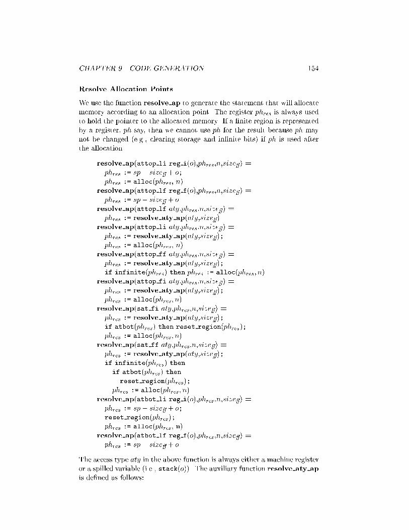
CHAPTER 9. CODE GENERATION 154
Resolve Allocation Points
We use the function resolve ap to generate the statement that will allocate
memory according to an allocation point. The register ph
res
is always used
to hold the pointer to the allocated memory. If a �nite region is represented
by a register, ph say, then we cannot use ph for the result because ph may
not be changed (e.g., clearing storage and in�nite bits) if ph is used after
the allocation.
resolve ap(attop li reg i(o),ph
res
,n,size
�
) =
ph
res
:= sp� size
�
+ o;
ph
res
:= alloc(ph
res
, n)
resolve ap(attop lf reg f(o),ph
res
,n,size
�
) =
ph
res
:= sp� size
�
+ o
resolve ap(attop lf aty,ph
res
,n,size
�
) =
ph
res
:= resolve aty ap(aty,size
�
)
resolve ap(attop li aty,ph
res
,n,size
�
) =
ph
res
:= resolve aty ap(aty,size
�
);
ph
res
:= alloc(ph
res
, n)
resolve ap(attop ff aty,ph
res
,n,size
�
) =
ph
res
:= resolve aty ap(aty,size
�
);
if infinite(ph
res
) then ph
res
:= alloc(ph
res
; n)
resolve ap(attop fi aty,ph
res
,n,size
�
) =
ph
res
:= resolve aty ap(aty,size
�
);
ph
res
:= alloc(ph
res
; n)
resolve ap(sat fi aty,ph
res
,n,size
�
) =
ph
res
:= resolve aty ap(aty,size
�
);
if atbot(ph
res
) then reset region(ph
res
);
ph
res
:= alloc(ph
res
; n)
resolve ap(sat ff aty,ph
res
,n,size
�
) =
ph
res
:= resolve aty ap(aty,size
�
);
if infinite(ph
res
) then
if atbot(ph
res
) then
reset region(ph
res
);
ph
res
:= alloc(ph
res
; n)
resolve ap(atbot li reg i(o),ph
res
,n,size
�
) =
ph
res
:= sp� size
�
+ o;
reset region(ph
res
);
ph
res
:= alloc(ph
res
, n)
resolve ap(atbot lf reg f(o),ph
res
,n,size
�
) =
ph
res
:= sp� size
�
+ o
The access type aty in the above function is always either a machine register
or a spilled variable (i.e., stack(o)). The auxiliary function resolve aty ap
is de�ned as follows:
CHAPTER 9. CODE GENERATION 155
resolve aty ap(ph,size
�
) = ph
resolve aty ap(stack(o),size
�
) = sp[�size
�
+ o]
9.2.3 Set Storage Modes
Storage modes are set when passing regions as arguments to letrec bound
functions, (e.g., when a region vector is constructed). The following speci�es
how the storage bits are set (phreg can be replaced by stack(o)).
attop li reg i(o): the atbot bit is not set so no change is necessary.
attop lf reg f(o): the region is �nite and the atbot bit is therefore in-
signi�cant.
attop lf phreg : the region is �nite and the atbot bit is therefore insigni�-
cant.
attop li phreg : even though the region is free to the function then the
atbot bit is not set because it is letregion bound. It is not necessary
to clear the atbot bit.
attop ff phreg : the region may or may not be in�nite so we have to check
the multiplicity and then clear the atbot bit if the multiplicity is in-
�nite. Actually, we may blindly clear the atbot bit no matter the
multiplicity.
attop fi phreg : the region is in�nite and we clear the atbot bit.
sat fi phreg : the atbot bit is already set appropriately.
sat ff phreg : the atbot bit is already set appropriately.
atbot li reg i(o): we set the atbot bit.
atbot lf reg f(o): the atbot bit is insigni�cant.
atbot li phreg : we set the atbot bit.
atbot lf phreg : the atbot bit is insigni�cant.
The atbot bit is never set on letregion bound regions when they are created
so we do not have to explicitly clear the atbot bit for those regions.
Resolve Storage Modes
The function resolve sm regvec sets or clears the atbot bit in regions
passed to region polymorphic functions as speci�ed in the previous section.
The function is given a temporary register t that is used if necessary.

CHAPTER 9. CODE GENERATION 156
resolve sm regvec(attop li reg i(o),t,size
�
) =
(t := sp� size
�
+ o;set inf bit(t),t)
resolve sm regvec(attop lf reg f(o),t,size
�
) = (t := sp� size
�
+ o; t)
resolve sm regvec(attop lf ph,t,size
�
) = (nop, ph)
resolve sm regvec(attop lf stack(o),t,size
�
) = (t := sp[�size
�
+ o]; t)
resolve sm regvec(attop li ph,t,size
�
) = (nop, ph)
resolve sm regvec(attop li stack(o),t,size
�
) = (t := sp[�size
�
+ o]; t)
resolve sm regvec(attop ff ph,t,size
�
) =
(t := ph; clear atbot bit(t), t)
resolve sm regvec(attop ff stack(o),t,size
�
) =
(t := sp[�size
�
+ o]; clear atbot bit(t), t)
resolve sm regvec(attop fi ph,t,size
�
) =
(t := ph; clear atbot bit(t), t)
resolve sm regvec(attop fi stack(o),t,size
�
) =
(t := sp[�f szie+ o]; clear atbot bit(t), t)
resolve sm regvec(sat fi ph,t,size
�
) = (nop, ph)
resolve sm regvec(sat fi stack(o),t,size
�
) = (t := sp[�size
�
+ o], t)
resolve sm regvec(sat ff ph,t,size
�
) = (nop, ph)
resolve sm regvec(sat ff stack(o), t) = (t := sp[�size
�
+ o], t)
resolve sm regvec(atbot li reg i(o),t,size
�
) =
(t := sp� size
�
+ o;set inf bit(t);set atbot bit(t),t)
resolve sm regvec(atbot lf reg f(o),t,size
�
) = (t := sp� size
�
+ o; t)
resolve sm regvec(atbot li ph,t,size
�
) =
(t := ph;set atbot bit(t),t)
resolve sm regvec(atbot lf ph,t,size
�
) = (nop,ph)
We note, that in many cases (e.g., when the access type is stack(o)) it
is possible to add the constants atbot bit and inf bit when the address is
calculated instead of using the set atbot bit and set inf bit primitives.
The constants must be de�ned such that they set the appropriate bit when
added.
9.2.4 Call Convention
The register allocation phase (Chapter 5) inserts statements around the
function calls such that arguments and results passed in registers are actually
put in the registers before the call and retrieved from the registers after the
call. However, it is the responsibility of the code generator to put arguments,
not passed in registers, on the stack and retrieve results, not passed in
registers, from the stack on return from the call. This section speci�es how
this can be done.
We need a convention for storing a call convention on the stack. A call
convention is split in three parts: a call convention frame (ccf), a return

CHAPTER 9. CODE GENERATION 157
�
caller
-
sp
�
caller
rcf
return lab
42
stack(2)
ccf
�
callee
-
sp
�
caller
stack(3)rcf
-
sp
6
Figure 9.4: At left we have the stack before the application. At center
we have the stack at entry to the called function and at right the stack
at return from callee. The stack grows upwards.
label
1
and a return convention frame (rcf). The call convention is allocated
before callee is called. On return from callee we have rcf allocated. Figure
9.4 shows the content of an example stack before an application, at entry to
a called function and at return.
A call convention uniquely speci�es which arguments and results are
passed on the stack and in what order. The method we use is to �rst
convert the application into a temporary call convention called the actual
call convention. We then use a function resolve act cc that, given an actual
call convention as argument, returns a statement that stores arguments into
the call convention frame (ccf) and a statement fetching results from the
return convention frame (rcf). The function also returns the size of the call
and return convention frames.
The actual call convention for an ordinary application
haty
1
; : : : ; aty
h
i := se
ck
hse
a1
; : : : ; se
an
i hse
c
i hse
f
1
; : : : ; se
f
m
i
or a region polymorphic application
haty
1
; : : : ; aty
h
i := lab
ck
hse
a1
; : : : ; se
an
i hse
r
i ha
1
; : : : ; a
l
i hse
c
i hse
f
1
; : : : ; se
f
m
i
is
acc = fclos= se
c
,
free= [se
f
1
; : : : ; se
f
m
],
args= [se
a
1
; : : : ; se
a
n
],
reg vec= se
r
,
1
We always put the return label on the stack. However, we believe it is better to let
the return label be an ordinary argument such that it can be passed in a register if the
register pressure is low.

CHAPTER 9. CODE GENERATION 158
reg args= [a
1
; : : : ; a
l
],
res= [aty
1
; : : : ; aty
h
] g
The function resolve act cc uses the same priorities as resolve cc on page
101 (and init F on page 137) to �nd the stack o�sets. Consider the appli-
cation
hph
9
; stack(3)i := lab
ck
hph
3
; 42; stack(2)i hph
2
i hi hph
1
i hi
with args phreg = [ph
1
; ph
2
; ph
3
] and res phreg = [ph
9
]. The corresponding
actual call convention is
acc = fclos= ph
1
,
free= [ ],
args= [ph
3
; 42; stack(2)],
reg vec= ph
2
,
reg args= [ ],
res= [ph
9
; stack(3)] g
Two arguments (42,stack(2)) and the result to go in stack(3) are passed
on the stack, see Figure 9.4. The function resolve act cc(acc) returns the
statement
pop(t);
sp[�size
�
+ 3] := t
that fetches the result from the return convention frame and the statement
push(42);
t := sp[�size
�
� 1 + 2];
push(t)
that stores the arguments in the call convention frame. We note that the
stack pointer is pointing at the �rst address after the current function frame
when the code to store arguments is executed. The stack pointer points at
the �rst address after the return convention frame when the code to fetch
results is executed. The o�sets used when accessing slots in the function
frame depends on the number of pop and push statements executed.
9.2.5 Functions
At entry to a function (either letrec or ordinary) we allocate the function
frame on the stack. The frame size (size
�
) is annotated on top level decla-
rations (computed in Chapter 7). The call and return convention is explicit
in the body of a function by either refering to machine registers or stack
positions directly. Arguments and results passed on the stack are referenced
directly with an o�set from the stack pointer. The stack annotations are

CHAPTER 9. CODE GENERATION 159
calculated in Chapter 7 and Figure 9.4 shows an example stack when calling
a function.
The code for the body of a function is organized as follows:
� code to allocate the function frame.
� code for the body of the function.
� code to return to the calling function by loading the return address
from the stack.
� code to set the stack pointer at the �rst address after the return con-
vention frame (i.e., rcf). The function frame for callee, call convention
frame (ccf) and return label is thus deallocated. Caller needs rcf to
fetch results passed on the stack.
Tail calls makes it necessary to deallocate both function and call conven-
tion frames before leaving the function; and not at the application point.
CG
T
[[�
fun(size
�
)
lab
cc => ls]] =
fun lab is
sp := sp+ size
�
;
CG [[ls]] size
�
size ccf(cc) ;
sp := sp� size
�
� size ccf(cc);
pop(t);
jmp t
Figure 9.5 shows the stack pointer at entry and exit of a function. The
function size ccf returns the size of the call convention frame (i.e., the
number of arguments pushed on the stack). An ordinary function (fn) is
translated likewise. Top level declarations are translated sequentially:
CG
T
[[top decl
1
;top decl
2
]] =
CG
T
[[top decl
1
]] ;
CG
T
[[top decl
2
]]
9.2.6 Applications
An ordinary application involves the following phases:
� store registers, that must be saved across the function call. This is
already done, see Chapter 6.
� allocate the return convention frame.
� push the return address on the stack. The code generator needs to
create a new return label.

CHAPTER 9. CODE GENERATION 160
�
caller
rcf
return lab
ccf
-
sp
�
caller
rcf
�
sp6
Figure 9.5: At entry to the function (at left), the stack pointer points at
the �rst free address after the call convention frame (ccf). At exit from
the function (at right), the stack pointer points at the �rst free address
after the return convention frame (rcf). The stack grows upwards.
� allocate the call convention frame.
� put arguments in machine registers or into the call convention frame as
speci�ed by the call convention. We only have to consider arguments to
go in the call convention frame. Arguments to go in machine registers
are resolved by the register allocator, see Chapter 5.
� jump to the function.
On return from the call we have to
� move the result values from the return convention frame into the places
(either machine registers or stack positions) where they are supposed
to be.
� the stack pointer points at the �rst address after rcf so we must deal-
locate rcf .
� fetch values that were stored across the function call. This is already
done, see Chapter 6.
The translation function for a function call to a region polymorphic
function is thus:
CG [[haty
1
; : : : ; aty
h
i :=
se
funcall
hse
1
; : : : ; se
n
i hse
reg
i ha
1
; : : : ; a
l
i
hse
clos
i hse
f
1
; : : : ; se
f
m
i]] size
�
=
let
val (st
args
; size
ccf
; st
res
; size
rcf
) = resolve act cc(fclos=se
clos
, : : : g)
val return lab = fresh lab("app")

CHAPTER 9. CODE GENERATION 161
val st
jmp
= resolve jmp(se; size
rcf
+ size
ccf
+ 1 + size
�
)
in
sp := sp+ size
rcf
;
push(return lab);
st
args
;
st
jmp
;
return lab: st
res
end
An application to an ordinary function is translated likewise. We use the
function resolve jmp to generate jump code depending on where the target
label is; either as a label constant or in a closure.
resolve jmp(lab; sp
adjust
) = jmp lab
resolve jmp(stack(o), sp
adjust
) =
t := sp[�sp
adjust
+ o];
t := t[0];
jmp t
resolve jmp(ph; sp
adjust
) =
t := ph[0];
jmp t
The constant sp
adjust
is the distance from top of ccf to the �rst address in
�
caller
, see Figure 9.5 at left.
Tail Calls
A tail call is simpler than an ordinary call because we do not return to caller
again; there are no more code to execute. We do not have to setup a return
convention frame and we shall not push a return address on the stack.
Because a tail call is an implicit return from the current function we
must deallocate the current function frame together with the current call
convention frame before jumping to the called function. We must also fetch
some callee save registers as explained in Chapter 6:
� fetch callee save registers.
� deallocate the current function frame.
� deallocate the current call convention frame.
� allocate a new call convention frame.
� put arguments into the call convention frame.
� jump to the function.

CHAPTER 9. CODE GENERATION 162
�
rcf
return lab
ccf
caller
�
caller
-
sp
�
rcf
return lab
�
callee
�
sp
6
Figure 9.6: At left we have the stack before a tail call. In the general
case we must deallocate �
caller
and ccf at the same time that we build
a new ccf for the called function. This is, in general, not possible to do
e�ciently so we make the assumption that all functions called in a tail
call may not have a ccf . At right, we have the stack at entry to the
called function. The stack grows upwards.
Figure 9.6 shows the stack before a tail call. If callee expects arguments on
the stack then we must overwrite ccf
caller
and �
caller
with ccf
callee
. However,
this is di�cult because both ccf
caller
and �
caller
may be needed when com-
puting the arguments (i.e., we cannot overwrite ccf
caller
and �
caller
while
building ccf
callee
). This may be solved by copying ccf
caller
into �
caller
at
entry to the caller and then reserve as much space between return lab and
�
caller
as is needed for all possible calls inside caller. The amount of space
needed is a local property of caller. We do not �nd this worth the trouble
because a tail call is not a fast call anymore. We decide to convert all tail
calls calling functions taking arguments on the stack into ordinary calls and
thereby keep tail calls fast. We do not believe this restriction to be a problem
because we have many argument registers. We make sure that algorithm F
(see Chapter 3) does not make functions non closure implemented if they get
more arguments than there are argument registers. If other analyses (like
unboxing records) also confer to this restriction then we will never convert
a tail call into a non tail call.
There is no restriction on the number of return values, that is, rcf may
always be used. We may weaken the restriction and use ccf
callee
in a tail
call in the case that ccf
callee
only contains actual region arguments being a
subset of the region arguments already in ccf
caller
, (see [49, Chapter 14]).
CG [[haty
1
; : : : ; aty
h
i :=
lab
funjmp(ls)
hse
1
; : : : ; se
n
i hse
reg
i ha
1
; : : : ; a
l
i
hse
clos
i hse
f
1
; : : : ; se
f
m
i]] size
�
size
ccf
=

CHAPTER 9. CODE GENERATION 163
if size act ccf(fclos=se
clos
, : : : g) > 0 then
CG [[haty
1
; : : : ; aty
h
i :=
lab
funcall
hse
1
; : : : ; se
n
i hse
reg
i ha
1
; : : : ; a
l
i
hse
clos
i hse
f
1
; : : : ; se
f
m
i]] size
�
size
ccf
else
CG [[ls]] size
�
size
ccf
;
sp := sp� size
�
� size
ccf
;
jmp lab
The statements ls fetches callee save registers, see Chapter 6. The callee
save registers are not fetched if the tail call is turned into an ordinary call.
Tail calls to ordinary functions are handled likewise.
9.2.7 Statements
In this section we show CG for some of the remaining statements. The
translation of statements not shown are similar to the translations shown.
They are all straight{forward given the previously de�ned functions.
CG [[aty := (se
1
; : : : ; se
n
)]] size
�
=
let
val (st
r
; r) = resolve aty def(aty, t
1
, size
�
)
val st
alloc
= resolve ap(a, r, n, size
�
)
val (t
i
; st
i
) = resolve se(se
i
; t
2
; size
�
)
in
st
alloc
;
st
1
;
r[0] := t
1
;
.
.
.
st
n
;
r[n� 1] := t
n
;
st
r
end
CG [[aty := [a
1
; : : : ; a
n
]
regvec
]] size
�
=
let
val (st
r
; r) = resolve aty def(aty, t
1
, size
�
)
val st
alloc
= resolve ap(a, r, n, size
�
)
val (t
i
; st
i
) = resolve sm regvec(a
i
; t
2
, size
�
)
in
st
alloc
;
st
1
;
r[0] := t
1
;
.
.
.
st
n
;

CHAPTER 9. CODE GENERATION 164
r[n� 1] := t
n
;
st
r
end
CG [[ls
1
; ls
2
]] size
�
size
ccf
=
CG [[ls
1
]] size
�
size
ccf
; CG [[ls
2
]] size
�
size
ccf
CG [[flush(aty,o)]] size
�
=
let
val (st; t) = resolve aty use(aty, t
1
, size
�
)
in
st;
sp[�size
�
+ o] := t
end
CG [[fetch(aty,o)]] size
�
=
let
val (st; t) = resolve aty def(aty, t
1
, size
�
)
in
t := sp[�size
�
+ o];
st
end
CG [[aty
1
:= #n(aty
2
)]] size
�
=
let
val (st
r
; t
r
) = resolve aty def(aty
1
, t
1
, size
�
)
val (st
s
; t
s
) = resolve aty use(aty
2
, t
1
, size
�
)
in
st
s
;
t
r
:= t
s
[n� 1];
st
r
end
CG [[letregioni o in ls end]] size
�
size
ccf
=
t
1
:= sp� size
�
+ o;
alloc region(t
1
);
CG [[ls]] size
�
size
ccf
;
t
1
:= sp� size
�
+ o;
dealloc region(t
1
)
CG [[aty
1
:= ::aty
2
]] size
�
=
let
val (st
r
; t
r
) = resolve aty def(aty
1
, t
1
, size
�
)
val (st
s
; t
s
) = resolve aty use(aty
2
, t
1
, size
�
)
in
st
s
;
t
r
:= cons tag(t
s
);
st
r
end
CG [[aty := se
1
bop se
2
]] size
�
=

CHAPTER 9. CODE GENERATION 165
let
val (st
r
; t
r
) = resolve aty def(aty, t
1
, size
�
)
val (st
s1
; t
s1
) = resolve se(se
1
, t
1
, size
�
)
val (st
s2
; t
s2
) = resolve se(se
2
, t
2
, size
�
)
in
st
s1
;
st
s2
;
t
r
:= t
s1
bop t
s2
;
st
r
end
CG [[case se
1
of c => ls
2
| => ls
3
]] size
�
size
ccf
=
let
val (st; t) = resolve se(se
1
, t
1
, size
�
)
in
st;
if (t = c) then
CG [[ls
2
]] size
�
size
ccf
else
CG [[ls
3
]] size
�
size
ccf
end
CG [[case se
1
of ::aty => ls
2
| => ls
3
]] size
�
size
ccf
=
let
val (st
s
; t
s
) = resolve se(se
1
, t
1
, size
�
)
val (st
r
; t
r
) = resolve aty def(aty, t
1
, size
�
)
in
st
s
;
if is cons(t
s
) then
t
r
:= decons(t
s
);
st
r
;
CG [[ls
2
]] size
�
size
ccf
else
CG [[ls
3
]] size
�
size
ccf
end
9.3 Example
The example function (fn xs) from page 147 is shown in Figure 9.7 translated
into KAM code.

CHAPTER 9. CODE GENERATION 166
fn fn xs is
sp := sp+ 14;
sp[�14 + 0] := ph
4
;
sp[�14 + 1] := ph
5
;
ph
4
:= ph
5
;
if (ph
2
= nil) then
ph
1
:= ph
4
[1]
else
if is cons(ph
2
) then
ph
1
:= decons(ph
2
);
ph
5
:= ph
1
[0];
t
1
:= ph
1
[1];
sp[�14 + 2] := t;
ph
2
:= sp� 14 + 12;
ph
2
[0] := sp� 14 + 7;
ph
2
[1] := sp� 14 + 3;
ph
3
:= ph
4
[2];
ph
1
:= ph
4
[3];
push(fold ret);
jmp foldl;
fold ret: ph
3
:= ph
1
;
sp[�14 + 11] := ph
3
;
ph
1
:= ph
4
[2];
ph
2
:= ph
5
;
push(fn ret1 );
t
1
:= ph
1
[0];
jmp t
1
;
fn ret1: ph
2
:= ph
4
[1];
push(fn ret2 );
t
1
:= ph
1
[0];
jmp t
1
;
fn ret2: ph
3
:= sp[�14 + 11];
ph
2
:= ph
1
;
ph
1
:= ph
3
;
push(fn ret3 );
t
1
:= ph
3
[0];
jmp t
1
;
fn ret3: t
1
:= sp[�14 + 2];
ph
2
:= t
1
;
push(fn ret4 );
t
1
:= ph
1
[0];
jmp t
1
;
fn ret4:
ph
4
:= sp[�14 + 0];
ph
5
:= sp[�14 + 1];
sp := sp� 14;
pop(t
1
);
jmp t
1
Figure 9.7: The function fn xs compiled into KAM code.

Part III
The Garbage Collector
167

Chapter 10
Basic Garbage Collection
Algorithms
In this chapter, we discuss basic garbage collection algorithms and introduce
a one phase and a two phase garbage collection abstraction. The immediate
di�erences between the algorithms presented are emphasized.
The chapter motivates the choice of garbage collector to use with region
inference. Region inference introduces several problems that are not found
in systems based solely on garbage collection and the choice of garbage
collector is therefore not obvious. A main di�erence is the number of heaps.
A system based on region inference does not have one or at most a small
bounded number of heaps but several maybe thousands, (i.e., each region has
its own region heap) and each region heap does not constitute a continuous
memory area but a list of linked region pages, see Chapter 2.
We illustrate some of the problems of measuring and comparing garbage
collection algorithms. These problems are relevant when evaluating our
implementation.
A comprehensive survey of garbage collection algorithms is found in Wil-
son's paper [58]. The survey has been very helpful both as a survey and as
a source of reference. The two phase garbage collection abstraction pre-
sented below is borrowed from the survey. Another excellent source is the
book \Garbage Collection { Algorithms for Automatic Dynamic Memory
Management", by Richard Jones and Rafael Lins [30].
10.1 Fundamentals
Garbage Collection may be de�ned in several ways and a de�nition often
used is that garbage collection is a mechanism which automatically reclaims
storage for the purpose of reuse. This is of course what we use garbage
collection for, but actually region inference does the same thing and the two
methods are very di�erent. It is better to characterize garbage collection
168

CHAPTER 10. BASIC GARBAGE COLLECTION ALGORITHMS 169
as an automatic and dynamic method for reclaiming storage for the purpose
of reuse. Region Inference is then characterized as an automatic and static
method for reclaiming storage for the purpose of reuse.
A static method does not interrupt program execution and is proba-
bly more time e�cient than a dynamic method. Allocation and dealloca-
tion statements are inserted into the program at compile time. A dynamic
method interrupts program execution and scans the memory to �nd the set
of values needed for the rest of the execution. This takes time but is also
more precise if the set of live objects can be determined precisely.
We use two simple garbage collection abstractions. The �rst abstraction
consists of two phases:
1. the detection or marking phase is the phase that splits the allocated
storage into a set of live objects
1
and a set of dead objects. This is
called the garbage detection phase [58].
2. in the second phase, we collect all dead objects and thereby free storage
for new objects to be allocated. This is called the garbage reclamation
phase [58].
As we will see, many garbage collection algorithms �ts into the above two{
phase abstraction. A one{phase abstraction is possible using two heaps:
1. �nd all live objects, and each time a new live object is found copy it
into a new heap. Afterwards the old heap may be freed.
An object is dead, opposed to live, if it is no longer needed by the running
program.
2
It is not necessarily the case that a garbage collector �nds all
dead objects, (i.e., conservative garbage collection). However, the set of
live objects must always contain, at least, all objects needed to �nish the
computation. If not, the garbage collector is not safe.
How do we split the memory into dead and live objects and ensure that
none of the live objects are deallocated? The set of live objects are normally
de�ned to be the set of objects that can be reached from a root{set. A
possible root{set contains globally de�ned variables, variables allocated in
activation records and registers. The root{set depends on when and where
the program may be interrupted and how the compiler is organized. The
root{set for the ML-Kit is de�ned in Chapter 13.
Given the set of live objects (Live) we require that:
1
In this section, we use the word object for one or more memory cells allocated as one
unit (e.g., a closure).
2
Note, that live as used in this chapter is di�erent from live used in liveness analyses,
see Chapter 5. If an object is needed by the program then it is de�ned live here. In the
liveness analyses, however, there may exists objects de�ned live by the liveness analysis
that are not needed by the program, (i.e., the liveness analysis is an approximation to live
as de�ned here).
CHAPTER 10. BASIC GARBAGE COLLECTION ALGORITHMS 170
for all obj 62 Live, the object obj cannot be reached by any
pointer traversal from any object live 2 Live.
If an object obj 62 Live can be reached from another object live 2 Live then
we cannot guarantee that obj is not needed to �nish the computation.
To �nd the set of live objects it is necessary to know whether or not a
given object contains scalars and/or pointers. For now, we assume objects
to be tagged with such information. Tagging in the ML-Kit is discussed in
Chapter 12.
We discuss two approaches to �nd the set of live objects. The �rst,
called reference counting is suitable for implementing real{time garbage col-
lection (i.e., the maximal program interruption time is bounded). The other
approach called tracing traverses memory starting from the root{set. The
algorithms presented here do not achieve real{time garbage collection but
can be modi�ed to do so.
10.2 Reference Counting
Reference counting [16] is a garbage collection technique which in its basic
version comes close to real{time collection. Each object holds a reference
count, which is the number of pointers pointing at the object.
An object is considered live, i� its reference count is not zero. The
reference count is initialized to one when the object is allocated for the �rst
time and incremented each time the object is allocated again (i.e., a new
pointer is pointing at the object).
An object is deallocated by decrementing the reference count, and the
object is reclaimed when the reference count reaches zero. The object being
reclaimed may point at other objects. If so the reference count of the \point
at" objects are decremented too, and if those reference counts reach zero they
must be reclaimed too. Deallocating an object may therefore start a series
of deallocations and reclamation of objects. This is why the basic reference
counting algorithm is not a real{time garbage collector; one deallocation
may lead to an unbounded number of deallocations. However, the problem
is easily solved with lazy deallocation. An object is deallocated by pushing a
reference to the object onto a stack of deallocated but non reclaimed objects.
References to objects are then popped from the stack and reclaimed with a
given frequency that cope with the real{time requirements. One possibility
is to reclaim one object at each allocation.
Garbage detection is performed by the bookkeeping of reference counts.
The garbage reclamation phase is when objects are deallocated. The book-
keeping of reference counts is limited to a small number of instructions but
they are executed every time an object is allocated and deallocated.
A reference count takes up space, and a word is necessary if a precise
bookkeeping of reference counts is needed. A shorter reference count �eld

CHAPTER 10. BASIC GARBAGE COLLECTION ALGORITHMS 171
can be used as for instance three bits with the counts 1 : : : 7 and 1. The
reference count 1 cannot be decremented and objects with the count 1
must be reclaimed with another garbage collection technique. A hybrid
garbage collector using a one{bit reference count and a tracing garbage col-
lector (e.g., mark{sweep or mark{compact, see the sections below) has been
proposed [59]. The idea is that while the tracing garbage collector is idle,
the mark bit may be used to distinguish between objects known to have a
reference count of one and objects having another reference count. Deallo-
cating an object with a reference count of one may be reclaimed instantly
whereas other objects are reclaimed by the tracing garbage collector. The
method delays the invocation of the tracing garbage collector signi�cantly
in environments where most objects are referenced only once.
In programs based solely on reference counting, it is necessary to make a
conservative approximation of the maximum number of possible references
to each object, when deciding the size of the reference count. This is in
general di�cult to estimate, especially for a compiler where it depends on
how the programmer uses the programming language being compiled. For
instance, in Standard ML, the function �a:(a; a) creates two references to a
each time the function is applied (we assume a represents a boxed value).
Manipulation of recursive data structures may create many pointers to the
same value. If we have the lists l
1
and l
2
then the function
fun splice l1 l2 = l1 @ l2
called with splice l
1
l
2
creates another pointer to the elements in list l
1
if
we use the implementation of @ as de�ned in SML90 [35].
3
The number of
pointers to the elements in l
2
remains the same except for the �rst element.
A major problem with reference counting is the inability to reclaim cyclic
structures. It is possible to have a cycle between two objects even though
there is no pointer from the root{set to the objects.
Cycles occur rarely in Standard ML, but here is an example showing
that they can occur, see Figure 10.1.
datatype cycle = A of cycle ref
| B of cycle ref
| None;
val res =
let
val n = None
val a = A (ref n)
val b = B (ref a) (* 1 *)
val _ = case a
of A(r) => r:= b (* 2 *)
3
The function is de�ned as fun nil @ M = M | (x::L) @ M = x::(L @ M).

CHAPTER 10. BASIC GARBAGE COLLECTION ALGORITHMS 172
res
-
(*1*)
A None
-
B
@
@I
res
�
(*2*)
A
�
�
B
@
@I
Figure 10.1: A possible representation of the values at the two situa-
tions (*1*) and (*2*). When the reference is updated the value None
will be deallocated, and hence freed.
| _ => print "Crash"
in
a
end
When the variable res is assigned the value of a (A) then the reference
count is two (from res and the value of b (B)). When res is deallocated
then the reference count for A is decremented to one. As no live value points
at A and the reference count is one, the values A and B are never reclaimed.
It turns out that a purely functional language creates cyclic data struc-
tures in a restricted manner, which can be treated specially and reference
counting is then applicable [7]. It is also possible to handle more general
circular structures, such as doubly linked lists. Each circular structure is
considered a single group. We have a reference count for each group and if
the count reaches zero then the entire group is deallocated [11].
The bookkeeping of reference counts puts a proportional factor on the
work done by the running program; the bookkeeping uses time on both
allocation and deallocation of objects. Reference counting may therefore not
be time e�cient, when there are many short lived values, which is common
in functional languages.
It is possible to defer the bookkeeping of local variables [18]. Instead of
updating reference counts on all objects we consider heap{allocated objects
only, that is, if a heap{allocated object points at another object then we
update the reference count. The reference count does not include pointers
from stack allocated objects. Instead of reclaiming an object when the
reference count reaches zero we insert the object in a list of potentially dead
objects. The stack is scanned with a given frequency and potentially dead
objects are only dead (and reclaimed) if they are not pointed at by any stack
allocated object.
Basic reference count algorithms consider the heap as one chunk of data.
Objects removed from the heap are inserted into one or more free lists.
Allocating an object involves searching the free lists.
The most important advantages of reference counting is the suitability for
real{time garbage collection and the fast reclamation of deallocated objects.

CHAPTER 10. BASIC GARBAGE COLLECTION ALGORITHMS 173
root
?
h
1
?
h
2
??
h
3
�
(a)
prev=nil
cur=h
1
root
?��
h
1
h
2
?
h
3
�
(b)
prev=h
1
cur=h
2
root
?��
h
1
6
h
2
6
h
3
(c)
prev=h
3
cur=nil
root
?��
h
1
6
h
2
h
3
�
(d)
prev=h
2
cur=h
3
Figure 10.2: The process of pointer reversal at four points in the al-
gorithm. Arrows pointing into \nowhere" represents nil pointers. We
assume the elements to be records with a �eld n donoting the pointer to
the next element.
10.3 Mark{Sweep Collection
A mark{sweep collector [34] �nds the live objects by following pointers from
a root{set. The objects reached are marked as live objects (i.e., detection of
live values). The heap is then sweeped for dead objects, that is, space not
occupied by marked objects is reclaimed (garbage reclamation) and inserted
in a free list.
The mark{sweep principle must perform at least two traversals of the
heap where the reclamation traversal (in its basic version) must touch every
address in the heap. As with reference counting, the heap is fragmented
in chunks of varying size containing either live or reclaimed objects. The
fragmentation problem is also known from explicit allocation by the pro-
grammer. For instance, the functions malloc() and free() are normally
implemented using one or more free lists containing chunks of reclaimed
objects of varying size [32, page 185].
To build the free lists it is necessary to search for the unmarked objects.
A scan through the entire heap may be necessary. The reclamation scan may
be optimized by building a data structure (for instance a bitmap) saying
where to �nd marked and unmarked objects while marking the live objects.
The marking phase involves considerable problems. A recursive algo-
rithm visiting nodes in either breadth or depth �rst order may run out of
stack space. An iterative algorithm pushing visited nodes on a stack for
later revisiting may also run out of stack space.
A linear and constant space algorithm can be obtained by using pointer
reversal. When traversing the heap, all branch points (i.e., objects with
unvisited children) must be saved somewhere for later revisiting. Pointer
reversal saves this information in the heap (i.e., in already allocated objects).
Consider Figure 10.2 with an example heap containing a single linked list.
While we traverse the list we reverse pointers such that we can go back
again.
Pointer reversal on a single linked list can be implemented using three

CHAPTER 10. BASIC GARBAGE COLLECTION ALGORITHMS 174
variables, prev, cur and next. Initially we have the situation in Figure 10.2(a)
with prev = nil and cur = root (i.e., h
1
). We then advance to the next
element (h
2
) by setting next = cur! n, cur ! n = prev, prev = cur and
cur = next. If variable v points at object o then we let v ! n be the �eld n
in o containing the pointer out of o. The pointer for h
1
is now reversed, see
Figure 10.2(b). We continue until the situation in Figure 10.2(c) is reached
and it is now possible to go back to h
1
from h
3
. We work back again by
setting next = prev ! n, prev ! n = cur, cur = prev and prev = next,
see Figure 10.2(d). We stop when the original heap has been reconstructed
(i.e., prev = nil). Additional ags (besides the mark ag) are needed when
objects contain more that one successor object but the method remains the
same.
4
Instead of storing mark bits in the headers of heap allocated objects
we can use an external bitmap and reserve one bit for each object with a
granularity corresponding to the smallest object allocated. On an 32 bits
machine with the smallest object being a word the bitmap size is
1
32
= 3:1%
of the heap space. On 64 bit architectures we have an overhead of 1:6%.
The sweep phase may be combined with allocation (lazy sweeping) [29].
The mark phase remains the same but we do not sweep the entire heap
and build free lists. Instead we sweep the heap imcrementally each time an
object is allocated by sweeping until an empty chunk of memory is found. If
none is found we initiate the marking phase and sweeps the newly marked
heap until a chunk of memory is found. The advantages are that no free lists
must be managed and the overall garbage collection delays are smaller. We
only need a global sweep pointer pointing at the address where the sweeper
should start next time.
Live objects spread through out the heap may invoke paging more often
than with a compacted heap (Section 10.4). The cache systems may also
su�er from having more global pointers and with an exhausted heap we may
initiate garbage collection more often because it is harder to accomodate the
allocation requirements than if all reclaimed objects were merged into one
larger chunk.
10.4 Mark-Compact Collection
A mark{compact collector solves the fragmentation problem of mark{sweep
collectors and thereby makes allocation faster.
Instead of sweeping the address space, the live objects are compacted
into one continuous block of memory. The rest of the memory area is then
4
A fun exercise is to implement the simple pointer reversal algorithm using two variables
prev and cur only and the identity (A�B)�B � A, where � is the exclusive{or operation.
The same identity can also be used to decrease the number of assignments in the algorithm
sketched above from four to three [45].

CHAPTER 10. BASIC GARBAGE COLLECTION ALGORITHMS 175
������������
������������
������������
������������
������������������
������������������
������������������
������������������
������������
������������
������������
������������
������������
������������
Dark cells contain live objects
����������
����������
����������
����������
���������������
���������������
����������
����������
���������������
���������������
���������������
���������������
����������
����������
alloc alloc and live meets
(a)
(b)
live
and white cells contain dead objects.
Figure 10.3: The two{�nger method traverses the heap in both direc-
tions looking for free space and live objects to relocate at the same time.
The initial heap is shown in (a) and (b) is after relocation. Note the re-
location pointers inserted in the relocated objects in the top half of the
heap. They are used when updating pointers in the bottom half (dark
area) of the heap.
freed.
The obvious advantages with compaction compared to sweeping are that
no free lists must be managed. Also, allocating objects is simpler as both
large and small objects are allocated from the same continuous area of mem-
ory. Only a pointer has to be moved in order to allocate an object. The
garbage collector is initiated when the allocation pointer exceeds the free
memory area.
However, as with a mark{sweep collector, two or more parses over the
address space are necessary. Many algorithms exists for compacting live
objects and we review three of them. For a more detailed comparison of
compacting algorithms including the calculation of symbolic time formulas
consult [15].
The two{�nger method [43] is simple and fast but in its basic version it
is suitable for �xed sized objects only. The �rst phase marks all live data.
The second phase scans the heap using two pointers, see Figure 10.3. The
alloc pointer starts at the bottom of the heap and looks for free space for
relocated objects. The live pointer starts at the top of the heap and looks
for live objects to relocate. Objects are relocated by copying them into the
space pointed at by alloc. After copying, the object pointed at by live is
overwritten with the new address pointed at by alloc. The copying ends
when the two pointers meet. Pointers in the bottom half are then updated
by traversing the bottom half and changing all pointers pointing into the
top half containing relocated objects, see Figure 10.3.

CHAPTER 10. BASIC GARBAGE COLLECTION ALGORITHMS 176
����������
����������
����������
����������
���������������
���������������
���������������
���������������
����������
����������
����������
����������
����������
����������
0 282 4 8 12 14 20 24 26
����������
����������
���������������
���������������
���������������
���������������
����������
����������
����������
����������
����������
����������
���������������
���������������
������������
������������
������������������
������������������
������������
������������
������������
������������
������������
������������
������������������
������������������
������������
������������
white cells contain dead objects.
����������
����������
����������
����������
���������������
���������������
����������
����������
���������������
���������������
����������
����������
���������������
���������������
(a)
(b)
(c)
(d)
0 282 4 8 12 14 20 24 26
0 282 4 8 12 14 20 24 26
(12,
6)
0 282 4 8 12 14 20 24 26
(12,
6)
(4,2
)
(4,2
)
(4,2
)
(20,
12)
(26,
14)
Dark cells contain live objects and
Figure 10.4: The break{table method inserts a break table into the free
cells in the heap. For each object moved, the old address of the object
together with the total amount of free space found so far is added to the
table. The new address of the object at address 20 is 20-12=8.
It is possible, allthough cumbersome, to implement the two{�nger method
with variable sized objects where di�erent sized compaction blocks are needed,
that is, one alloc pointer for each object size is needed.
The next method uses a break table stored in the free address space in the
heap [26]. The break table contains enough information about the relocated
objects in order to update pointers pointing at relocated objects. First live
objects are marked. The next phase moves objects and builds the break
table that, for each object moved, contains the start address of the object
before moving and the total size of free space found so far (i.e., (addr; size)),
see Figure 10.4. There is always free space for the break table as long as one
table entry (pair) is smaller than the smallest heap{allocated object [26]. As
objects are moved toward lower addresses it is necessary to move the break
table toward higher addresses. This can be done by rolling the table such
that only fractions of the table is moved for each relocated object. When
all objects are moved the table is sorted after address of object (i.e., addr).
Addresses pointing at relocated objects are resolved by scanning the
compacted half of the heap and for each pointer p �nd the entries (a
1
; s
1
)
and (a
2
; s
2
) in the break table such that a
1
� p < a
2
. The new address for p
is then p� s
1
. For instance, in Figure 10.4 the new address of the relocated
object at address 26 is 26-14=12.

CHAPTER 10. BASIC GARBAGE COLLECTION ALGORITHMS 177
InfoA
A
��������
����
B
InfoB
C
����
��������
����
����
InfoC
B
InfoB
C
InfoA
A
InfoC
(b)(a)
Figure 10.5: The original heap is shown in (a). After threading, the
header �eld of object C (infoC ) is moved into the pointer �eld of object
A and a pointer to object B is stored in the header �eld in C. Updating
the pointers to C in A and B is then done by following the pointer out
from C.
The complexity of the algorithm is O(n logn) due to the sorting and
searching into the break table (n is the size of the heap). However, in
practice an almost linear complexity can be engineered [25].
The last compacting method we discuss is based on threading and is
related to pointer reversal used for marking live objects [24, 31]. Suppose
we have two objects A and B pointing at another object C, see Figure
10.5(a). If we move object C then the pointers into C must be updated with
the new address of C. This can be done easily by �rst building the structure
in Figure 10.5(b). Given object C we know which objects are pointing at C
and can easily update the pointers with the new address of C without loss
of information including the header �eld in object C. The update of some
or all addresses is done before objects are moved to their new locations.
Besides marking live objects, a forward and backward scan of the heap
are needed (i.e., complexity O(n) where n is the size of the heap). The for-
ward pass handles forward pointing pointers and the backward scan handles
pointers pointing backwards, consult [31] for further detail. The method
assumes that pointers only point at the header of other objects. This is
always the case in the ML Kit. However, the method also assumes that a
header �eld is large enough to contain an address (necessary for threading)
and that the address is distinguishable from non addresses. This is not the
case in the ML Kit. For instance, nullary value constructors occupy one
word only even if tagging is enabled, see Chapter 12.
10.5 Copying Garbage Collection
A simple copying garbage collector (called stop and copy) [23] uses two
address spaces, also called semi spaces. Only one semi space is used at the

CHAPTER 10. BASIC GARBAGE COLLECTION ALGORITHMS 178
time (i.e., the current semi space) in which objects are allocated. Garbage
collection is initiated when the current semi space is full. Live objects are
traversed and copied from the current semi space (also called the from{space)
into a new semi space, called the to{space. The copied objects are compacted
in the to{space. After copying an object, the �elds in the copied{from
object are replaced with forward pointers pointing at the �elds in the new
object in to{space. We assume that forward pointers can be distinguished
from other pointers and values. For each object traversed in from{space we
know whether or not the object has already been copied and if an instance
already exists in to{space then a forward pointer tells us the new address
of the object. The live objects in from{space are copied exactly once. After
all live objects in from{space has been traversed, we let to{space be the
current semi space and the from{space is not used until garbage collection
is initiated again. As pointers are updated when objects are copied into
to{space, only one scan of the live objects is needed.
As with mark{compact collectors, there is no fragmention and allocation
is done e�ciently by moving an allocation pointer.
We allocate about twice the memory necessary for the running program
which may be a problem for some memory demanding programs. The virtual
memory systems used in modern computers [42, 28] partly solves the prob-
lem by swapping the non current semi space out of memory when memory
demand is high. However, the time involved in paging and swapping may
be signi�cant descreasing the overall performance of simple stop and copy
algorithms
10.5.1 Simple Stop and Copy
In this section we describe a simple stop and copy algorithm based on recur-
sion [23]. Cycles are easily handled by marking each object with a visited
ag. When an object is �rst met, the mark is set. The mark is then checked
to see whether or not an object has already been visited. However, assuming
we can distinguish forward pointers from other pointers and non pointers
then the forward pointers gives us the same information as a mark ag. This
only requires that all �elds in an object are updated with their new forward
pointers before decendants of the object are traversed. Consider the object
# 4 #
with two pointer �elds and a scalar �eld.
5
When the object is �rst met we
make a new instance of the object in to{space, and update all three �elds
in the from{space object with forward pointers into the �elds of the new
to{space object. We then recursively traverse the pointer objects in the
to{space object. Note that if pointers always point at the start of an object
then we only need one forward pointer for each object.
5
We use # to denote pointers and numbers to denote non pointer �elds.

CHAPTER 10. BASIC GARBAGE COLLECTION ALGORITHMS 179
root{set
v
1
5
?
v
2
-
?
v
3
�
�
v
4
4
Figure 10.6: Pointer �elds are shown with arrows and scalar �elds with
their scalar value. The root{set consists of the object v
1
.
root{set
v
1
5
?
v
2
-s
-s
v
0
2
-
�
�
�
v
3
�
6
v
4
4
Figure 10.7: Forward pointers are shown as arrows with a �lled circle.
The two semi spaces to{space and from{space are not shown. We assume
objects named with a \pling" (e.g. v
0
2
) to be allocated in to{space and
other objects to be allocated in from{space.
We assume that root{set objects are never moved and therefore always
leave pointers into root{set objects unchanged. However, this depends on
the application.
Consider the example heap in Figure 10.6. The root{set object contains
one pointer �eld pointing at v
2
. A copy of v
2
is put in to{space named v
0
2
,
and the two pointer �elds in v
2
are changed into forward pointers, see Figure
10.7.
The �rst pointer �eld in v
0
2
is then traversed which �rst produces a new
instance of v
3
. Forward pointers are put in v
3
, see Figure 10.8.
The �rst pointer �eld in v
0
3
points at the root{set object and is left
unchanged. The second pointer �eld in v
0
3
points at a forward pointer in
v
2
and is updated accordingly. We are now done with object v
3
and return
the address of object v
0
3
so that the pointer object in v
0
2
can be updated, see
Figure 10.9.
The second pointer �eld in v
0
2
is then traversed and a copy of v
4
is
allocated in to{space (v
0
4
). The scalar �eld in v
4
is replaced by a forward
pointer to v
0
4
. The address of v
0
4
is returned and the second pointer object in

CHAPTER 10. BASIC GARBAGE COLLECTION ALGORITHMS 180
root{set
v
1
5
?
v
2
-s
-s
v
0
2
-
�
�
�
v
3
-s
-s
v
0
3
�
6
v
4
4
Figure 10.8: The object v
3
has been copied into to{space (v
0
3
) and
forward pointers are put in v
3
. Note, that there are no changes to object
v
0
2
yet.
root{set
v
1
5
?
v
2
-s
-s
v
0
2
@
@R
�
�
�
v
3
-s
-s
v
0
3
�
6
v
4
4
Figure 10.9: The �rst pointer �eld in v
0
2
is updated after return from
object v
3
. Note the change in the second pointer �eld in object v
0
3
.

CHAPTER 10. BASIC GARBAGE COLLECTION ALGORITHMS 181
root{set
v
1
5
@
@R
v
2
-s
-s
v
0
2
@
@R
?
v
3
-s
-s
v
0
3
�
6
v
4
-s
4 v
0
4
Figure 10.10: Objects with forward pointers may now be freed.
v
0
2
is updated to point at v
0
4
. We are now done with v
2
and the address of v
0
2
is returned to v
1
and the pointer �eld is updated to point at v
0
2
, see Figure
10.10. The objects v
2
; : : : ; v
4
residing in from{space may now be freed.
The following C function implements the algorithm sketched above with
the restriction that pointers must point at the start of an object. The pointer
objPtr points at a live object.
int gc(int *objPtr ) f
int *new , *i ;
if is in root set(objPtr)
return (int)objPtr ;
else f
if is forward ptr(*objPtr )
return clear forward ptr (*objPtr);
else f /* We point at an unvisited object */
new = copy val(objPtr);
for(i=�rst obj ptr (*new),i ,i=next obj ptr (i))
if is ptr (*i)
*i = gc(*i); /* Update �eld i. */
return (int)new ;
g
g
g
The function copy val(objPtr) copies the object pointed at by objPtr and in-
troduces forward pointers. The function is in root set(objPtr ) tests whether
or not objPtr points at a root{set object and the function is forward ptr (*objPtr)
tests wheter or not the point at object is already copied. If it is copied
then the forward pointer is returned after clearing the bit that identi�es the
pointer as a forward pointer. The loop runs through all �elds in the copied
object and calls gc recursively on all pointer �elds.

CHAPTER 10. BASIC GARBAGE COLLECTION ALGORITHMS 182
root{set
v
1
5
�
v
2
X
X
X
X
X
X
X
X
X
Xy
s
X
X
X
X
X
X
X
X
X
Xy
s
v
3
�
6
v
4
4
to{space
v
0
2
s
-
a
-
@
@
@
@R
-
Figure 10.11: We loop over the to{space area to collect the live values.
The scan pointer s points at the next �eld to collect.
Recursion is expensive because we perform a function call for each live
pointer value in the heap. It takes time to setup a function frame with
temporary values etc. A deep call tree may invoke a fatal error by exhausting
the stack. Data structures, as large search trees, in Standard ML may create
a deep call tree with the above method.
10.5.2 Cheney's Algorithm
The disadvantages of recursion are easily avoided using the to{space area
to record the values that have been copied but not collected yet [14]. We
do a breadth �rst traversal instead of a depth �rst traversal as the recursive
algorithm above.
The algorithm uses an allocation pointer a and a scan pointer s both
pointing into the to{space area. The allocation pointer points at the address
where the next relocated object is stored. The scan pointer points at the
current object (or �eld) being garbage collected. Each time an object (or
�eld) is collected the scan pointer is adjusted to point at the neighbor object
(or �eld). The algorithm ends when s = a.
Consider the example heap in Figure 10.6 again. The root{set object
v
1
is not copied into to{space. The �rst value we copy is v
2
and then we
scan the to{space area and collect all other live values. As in the recursive
algorithm we insert forward pointers when copying v
2
. We also update the
pointer �eld in v
1
to point at v
0
2
, see Figure 10.11
The next �eld to collect, pointed at by s, is an object pointer pointing
at v
3
. The value v
3
is copied into to{space, see Figure 10.12.
The second object pointer in v
2
points at a scalar object that is copied
into to{space. The �rst pointer object in v
0
3
points at the root{set value
and is left unchanged. The second object pointer in v
0
3
points at a forward
pointer and is updated accordingly. Now the scan pointer points at the
scalar object which is left unchanged. The algorithm stops when a = s, see

CHAPTER 10. BASIC GARBAGE COLLECTION ALGORITHMS 183
root{set
v
1
5
�
v
2
X
X
X
X
X
X
X
X
X
Xy
s
X
X
X
X
X
X
X
X
X
Xy
s
v
3
P
P
P
Pi
s
P
P
P
Pi
s
�
�
�
�
�
�
�
�
�
�:
6
v
4
4
to{space
v
0
2
s
�
a
-
�
-
v
0
3
Figure 10.12: The �rst �eld in v
0
2
is now collected and afterwards s
points at the second object pointer in v
0
2
.
root{set
v
1
5
�
v
2
X
X
X
X
X
X
X
X
X
Xy
s
X
X
X
X
X
X
X
X
X
Xy
s
v
3
P
P
P
Pi
s
P
P
P
Pi
s
�
�
�
�
�
�
�
�
�
�:
�
v
4
4
-s
to{space
v
0
2
a; s
�
��
-
-
v
0
3
Figure 10.13: The objects v
2
; v
3
and v
4
may now be freed.
Figure 10.13.
The algorithm is fast because it is driven by a simple loop. First we loop
through the root{set values and copy the initial objects into to{space. Then
we loop over the to{space area until all objects have been collected; there
are no other external structure that has to be updated. Note, that we can
not deallocate objects containing forward pointers in from{space before all
values in to{space have been collected. The overall algorithm is as follows:
1. a = �rst addr in to space
2. 8 objPtr 2 root set : *objPtr = gc(*objPtr);
3. for(s=�rst addr in to space;s<a;s++) if (is ptr(*s)) *s = gc(*s);
4. make to{space the current semi space.
The function gc is slightly di�erent from the recursive algorithm.
int gc(int *objPtr ) f
if is in root set(objPtr ) then

CHAPTER 10. BASIC GARBAGE COLLECTION ALGORITHMS 184
return objPtr ;
else f
if is forward ptr (*objPtr) then
return clear forward ptr (*objPtr);
else /* We point at an unvisited value */
return copy val(objPtr);
g
g
The funtion copy val ajusts the allocation pointer.
10.5.3 Generational Garbage Collection
A copying garbage collector is e�ective on small objects with a short life
time; an object with a life range that starts and ends between two successive
garbage collections is collected for free. However, large objects with a longer
life range are expensive because they are copied at each collection. Especially
global data are copied over and over again.
Generational garbage collection solves this problem in the case that most
objects allocated have a short life range and the number of pointers from old
objects into newer objects are small. An older cell can point to a newer cell
if the older cell is modi�ed after it is created. This is only possible through
references in Standard ML.
The heap is divided into a number of generations, G
1
; : : : ; G
n
and the
newest generation G
1
is garbage collected most often. As objects survive
garbage collections they get older and are eventually copied into older gen-
erations that are collected less often. Given a root{set a naive algorithm
must traverse all live objects including objects in older generations in order
to �nd all live objects in the younger generations. It is better if we can limit
the search to include younger generations only. This is possible if there are
no pointers from an older generation into a younger generation. Each time
we have a pointer into an older generation we then stop traversing. However,
with references in Standard ML we may have references from older gener-
ations into younger generations, but they are relatively rare. In SML/NJ
[5] the problem is solved by maintaining a list of addresses of cells in older
generations which have been updated after they were created. Letting the
list be part of the root{set we are sure to get all live data in the younger
generations and still only traverse the younger generations. This is only
e�cient because the list in practice is small.
The Caml Light garbage collector [44] is generational with two genera-
tions and hybrid using a stop and copy collection of the young generation
and incremental mark{sweep collection of the old generation. The mark{
sweep collector reduces the time used on copying because older objects are
not moved.

CHAPTER 10. BASIC GARBAGE COLLECTION ALGORITHMS 185
10.6 Comparing The Algorithms
We have chosen the criterias below as a basis for comparing the basic garbage
collection algorithms described in this chapter.
User interaction tolerance: for how long time and how often is the user
program interrupted.
Reference counting gives small but many user interactions which may
give the impression of a smoother program execution compared to
the tracing algorithms with fewer but longer interactions. It is easier
to have reference counting ful�ll some real{time requirements than a
tracing algorithm. The lazy sweeping method [29] improves the basic
mark{sweep method but still has to trace all live data. Both reference
counting and the tracing algorithms can be made incremental but
their implementations and especially tracing algorithms tend to be
complicated.
We do not consider real{time properties to be important for the garbage
collector in the ML Kit. Garbage collection is an add on only and re-
gion inference is the main memory allocation strategy which handles
most real{time requirements. Small real{time applications should be
developed using region inference only.
Precision criteria: how precise is the algorithm in reclaiming dead ob-
jects.
Reference counting does not reclaim cyclic structures. All tracing algo-
rithms reclaims all but live data i� a precise root{set can be calculated.
We want the garbage collector in the ML Kit to reclaim all garbage
based on the root{set given, that is, we want cyclic structures to be
reclaimed properly.
Aggressiveness: for how long time are objects allocated after they have
died.
Reference counting is aggressive because an object is reclaimed as soon
as the count reaches zero. Tracing algorithms wait until they are trig-
gered by, for instance, an exhausted heap. Region inference shares
the eagerness of reference counting where entire regions are relaimed
as soon as they are inferred to be dead. The only di�erence is that
reference counting is dynamic and region inference is static. Region
inference already recycles the heap e�ciently [10, 49]. We expect re-
gion inference to recycle most of the allocated memory such that the
rate in which memory is �lled with dead objects is low.
Root{set computation: the tracing algorithms need to compute a root{
set. It is possible to compute a root{set in the ML Kit, see Chapter
13.

CHAPTER 10. BASIC GARBAGE COLLECTION ALGORITHMS 186
Tag information: what kind of tagging is necessary to implement the al-
gorithm.
Reference counting requires several bits for the reference counts op-
posed to the tracing algorithms which need a single bit only (for each
word) to di�erentiate between scalars and pointers.
6
This is indeed a
serious drawback of reference counting in our framework because we
have a large number of objects. The problem tends to disappear when
the number of objects gets smaller as for instance in �le systems where
the number of open �les is easily handled using reference counting. A
�le descriptor is reclaimed when the reference count reaches zero.
Overhead/performance: what kind of overhead is imposed by the algo-
rithm and what is the asymptotic performance complexity. We note
that complexity formulas involving constants must be read carefully
because, the size of the constants may be more important than the
actual complexity. This is indeed the case with garbage collection al-
gorithms. All algorithms we have presented are linear (in the size of
live data or the heap) except for the break table method with com-
plexity n logn, where n is the size of the heap.
Say that allocating an object gives overhead a, then if it is done often
it is signi�cant whether the constant is large or small.
Let H be the size of the heap and let U be the amount of allocated
(used) memory, (i.e., U � H). Let N be the number of times an object
is allocated (and deallocated).
The time used on reference counting is t
RC
= c
1
N , where c
1
is time
used on allocation and deallocation including bookkeeping of reference
counts and free lists.
The mark{sweep method uses time t
MS
= c
2
U + c
3
H where c
2
is the
time used on allocation and tracing the heap and c
3
is the time used
on sweeping. Using lazy sweeping the term c
3
H dissapears from t
MS
and the overhead c
2
also includes the searching for a chunk of memory.
With lazy sweeping the complexity depends on live objects only and
not the size of the heap, as is the case for mark{compact collectors.
The mark{compact method uses time t
MC
= c
4
H log c
5
U using the
break table method and t
MC
= c
6
H using threading. The constant c
4
includes time to move objects, update pointers and roll the break table.
The constant c
5
is the overhead in sorting and searching the break
table. The constant c
6
includes the work of threading and unthreading
pointers.
6
The presentation is simpli�ed because a single bit is not always enough to di�erentiate
between scalars and non scalars, see Chapter 12. But it is still, by far, better than reference
counts.

CHAPTER 10. BASIC GARBAGE COLLECTION ALGORITHMS 187
The copy method uses time t
C
= c
7
U where c
7
includes the time used
to copy live objects and update forward pointers.
Allocation is more expensive for mark{sweep collectors based on free
lists than for compacting collectors. This is important in Standard
ML where the allocation frequency is high and the average life range
small. The SML/NJ'0.93 compiler reclaims, in average, 98.7% of the
heap at each garbage collection [5, page 206]. The compating collectors
use time proportional to the heap size and not the size of live data.
This favors the copying method except in the case where we have large
objects with longer life ranges. This is however not the average case
in Standard ML programs where most objects allocated are tupples
and closures.
Implementation: considering the region heap (being a linked list of region
pages) it is di�cult to see how an e�cient allocation strategy is based
on free lists. We then need a free list for each allocated region.
Region inference makes most regions contain objects of the same size.
However, some regions do not and the two{�nger method is therefore
not suitable.
The threading algorithm assumes that all objects have a pointer sized
header �eld. We believe this to be an expensive restriction especially
due to the large amount of constructors that can be implemented using
one word only.
The break table method assumes the smallest heap allocated object
to be of size two words. This is not the case in the ML Kit where
for instance a nullary value constructor occupies one word only. It is
still possible to use the method with the cost that not all garbage may
be removed [25]. The region heap also complicates the break table
method signi�cantly because the break table must be rolled between
di�erent non continuous region pages.
The simple recursive copy method works with the region heap as long
as we can allocate into the region heap. Let each region have two lists
of region pages, a from{list and a to{list. After garbage collection we
free all from{lists and, for each region, make the to{list the current
list of region pages. This also minimizes the overhead of data used.
Instead of having an overhead of one semi space the overhead is the
number of region pages used to hold live data.
We believe the most promising choice for the ML Kit is a copying garbage
collector. It is simple to implement, works with regions and only needs a
minimum amount of tagging. We re�ne the Cheney method to work with
regions in Chapter 11.

Chapter 11
Garbage Collection of
Regions.
In Chapter 10 we found the most promising garbage collection method for
regions to be simple non generational copying garbage collection. In this
chapter we show how the copying priciple developed by Cheney [14] is ex-
tended to work with regions. We also describe extensions to region descrip-
tors and region pages.
11.1 Algorithm Using Recursion
It is easy to re�ne the simple recursive copying garbage collector from Section
10.5.1 to work with regions. The algorithm does not put restrictions on the
number of to{spaces and from{spaces.
We extend the in�nite region descriptors to hold an additional list of
region pages so that each region has its own from{space and to{space. An
in�nite region descriptor then contains the following �elds (consult [22] for
more information about each �eld in the descriptor):
1. allocation pointer (a), which points at the next available address in the
region page currently being allocated into. When garbage collecting,
a points into to{space, and otherwise a points into from{space.
2. pointer to the �rst region page (fp) in from{space.
3. pointer to the end of the region page currently being allocated into.
This is called the border pointer, b. The pointer b points at the border
of to{space when garbage collecting and otherwise at the border of
from{space.
4. pointer to the previous region descriptor on the region stack, p.
5. pointer to the �rst region page in to{space, (fp' ).
188

CHAPTER 11. GARBAGE COLLECTION OF REGIONS. 189
fp
b
a
fp'
p
(a)
-
?
0
66
-
?
fp
b
a
fp'
p
(b)
-
?
0
??
-
0
?
Figure 11.1: Part (a) shows an example region descriptor with from{
space (fp) and to{space (fp' ) at a time where garbage collection is not
performed. Values are allocated in from{space. The pointer fp' may
point at anything. Part (b) shows what happens during garbage col-
lection. The allocation and border pointers now work on the to{space.
After garbage collection the from{space region pages are freed and the
to{space region pages are turned into from{space region pages.
We note that it is not necessary to have two instances of the allocation
and border pointers because at any time we either allocate into from{space
or into to{space. The region pages in from{space contain garbage after a
garbage collection phase and are moved to the free list for recycling. The
pointer fp is then set to point at to{space, that is, to{space is then the
current space in which objects are allocated, see Figure 11.1.
11.2 Cheney's Algorithm and Regions
Cheney's algorithm from Section 10.5.2 does not, as is, work with regions
because we do not have a single to{space but an unbounded number of to{
spaces, that is, an unbounded number of scan and allocation pointers. The
algorithm ends when all scan and allocation pointers are equal. The stop
criteria is then a �xed point criteria:
8r 2 Reg : r! a = r ! s;
where Reg is the set of in�nite region descriptors on the region stack, r! a
is the allocation pointer and r ! s is the scan pointer in region r. A
naive implementation of the �xed point criteria looping through all region
descriptors on the stack is indeed not an e�cient solution. There may only
be a small number of regions not ful�lling the stop criteria.
Consider Figure 11.2 with a data structure that imposes an interesting
behavior on Cheney's algorithm extended to regions. At any time during
garbage collection, at most two regions will contain one copied and non
collected value. With the naive implementation of the �xed point criteria
the region stack is traversed for almost every copied value, see Figure 11.3.

CHAPTER 11. GARBAGE COLLECTION OF REGIONS. 190
elem
record tag
?
6
elem
NIL
record tag
?
6
CONS
?
CONS
?
CONS
?
�
elem
�
rec
�
cons
Figure 11.2: The �gure shows an example data structure allocated in
three regions. It is a possible implementation of lists where cons and nil
cells are allocated in �
cons
, records in �
rec
and elements in �
elem
. We
note that lists are implemented more e�ciently in the ML Kit and that
this �gure serves only as an illustration.
CONS
s
6
a
6
a; s
6
a; s
6
(a)
CONS
a; s
6
record
s
6
a
6
a; s
6
(b)
CONS CONS
s
6
a
6
record
a; s
6
elem
s
6
a
6
(c)
CONS CONS
a; s
6
record record
s
6
a
6
elem
a; s
6
(d)
�
elem
�
rec
�
cons
Figure 11.3: It may be necessary to loop through the region stack many
times because only a fraction of the set of live values in a region is copied
into to{space each time the region is collected. Scanning region �
cons
gives one new value in �
rec
, (a)!(b). Scanning region �
rec
gives one new
value in �
cons
and �
elem
, (b)!(c). Scanning �
elem
does not introduce
new values but scanning �
cons
introduces one new value in �
rec
, (d).

CHAPTER 11. GARBAGE COLLECTION OF REGIONS. 191
CONS
sp
-
(a)
record
sp
-
(b)
CONS
elem
sp
-
(c)
record
elem
sp
-
(d)
NIL
elem
elem
sp
-
(e)
sp
-
(f)
Figure 11.4: The �gure shows seven snapshots of the scan stack (a)
{ (f) when collecting the data structure in Figure 11.2. The maximal
height of the stack is n+1 where n is the number of elements in the list.
11.2.1 A Stack of Values
The problem with more than one to{space is avoided using a scan stack
containing pointers to values copied into to{space areas but not traversed
yet. Each time a value is copied into to{space, a pointer to the value is
pushed on the scan stack.
It is not necessary to have a scan pointer in each region descriptor, and
not even on the scan stack. We simply pop the top pointer and collect the
value it points at. We are done when the scan stack is empty.
There is a small overhead for each copied value in both time and space
compared to Cheney's algorithm, but it solves the problem of having many
to{spaces. There is no recursion and the algorithm is not vulnerable to
recursive data structures. However, many objects may be pushed on the
scan stack at the same time. This extra space usage is a fatal problem.
Figure 11.4 shows the scan stack while collecting the data structure in Figure
11.2.
11.2.2 A Stack of Regions
Instead of storing pointers to values in the scan stack we can store pointers
to region descriptors containing non collected values [47].
Consider the region descriptor in Section 11.1, Figure 11.1. We extend
the region descriptor with a region status:
NONE if there are no non collected values in to{space.
SOME(s) if there are non collected values in to{space. The
pointer s then points at the next non collected value in
to{space (i.e., s is the scan pointer).
Each time a value (v) is copied into to{space (v
0
), the region status is
checked, and if NONE, then the status is changed into SOME(a) where
a is the allocation pointer pointing at the address where v
0
is stored. A
pointer to the region is pushed onto the scan stack. If the region status is

CHAPTER 11. GARBAGE COLLECTION OF REGIONS. 192
�
1
fp
b
a
fp'
p
-
v
2
?
0 v
3
66
-
?
? ?
6
v
1
5
6
?
�
2
fp
b
a
fp'
p
-
4 v
4
0
6
6
-
�
Figure 11.5: We have drawn the values v
2
; v
3
and v
4
as allocated in
the two regions. The region �
1
has two region pages allocated with a
value in each one and a pointer to the next region page. A null pointer is
written 0. We have not drawn the backward pointer from a region page
to the region descriptor. Only one region page is necessary in region �
2
.
The value v
1
is allocated on the stack and is in the root{set.
SOME(ptr) then nothing is done, because the value v
0
is automatically col-
lected next time the pointer to the region descriptor is popped from the scan
stack. The region status of the region currently being collected is changed
to NONE when we are done with the region. This prevents the region to be
pushed on the scan stack while it is actually being collected.
A minor optimization is to push the scan pointer on the scan stack
directly (instead of a pointer to the region) and then only manage a status
bit in the region descriptor. We use Cheney's algorithm locally on each
region and are done when the scan stack is empty.
The algorithm is best illustrated on our running example in Figure 10.6
on page 179. Assume we have two regions, �
1
and �
2
, where value v
2
and
v
3
are allocated in �
1
and value v
4
is allocated in �
2
, see Figure 11.5.
To initialize the scan stack we collect all values in the root{set (i.e.,
v
1
). This may cause values allocated in regions, to be copied into to{spaces.
After initialization, all regions containing values in to{spaces will have the
region status SOME(ptr) and are pushed on the scan stack.
Unfortunately, we must check the region status each time we copy a
value. This is only feasible if we, given a pointer to a copied value inside a
region page, can �nd the region descriptor holding the region status. This
is done by having all region pages of �xed size and aligned. Given a pointer
(val ptr) into a region page, the start of the region page is found by masking
out the o�set (val o� ) of the pointer relative to the base address (base ptr)
of the region page.
Say that each region page has size 1 Kb. and is aligned at 1 Kb. ad-
dresses. The �rst 10 bits of the base pointer to the region page are then
zero. Every pointer into the region page then consists of the base pointer

CHAPTER 11. GARBAGE COLLECTION OF REGIONS. 193
�
1
fp
b
a
fp'
p
S
-
v
2
?
0 v
3
-
v
0
2
0
6
?
s
?
s
6
6
6
v
1
5
6
?
�
2
fp
b
a
fp'
p
N
-
4 v
4
0
-
scan stack
sp
-
-
Figure 11.6: We reduce pointer spaghetti by not drawing the border, al-
location and previous region descriptor pointers. The status SOME(ptr)
is drawn as S. Likewise, the status NONE is drawn N. The scan stack
contains region �
1
. Forward pointers are drawn with a bullet.
plus an o�set which is held in the �rst 10 bits:
base ptr = val ptr AND 0
31
� � � 0
10
1
9
� � � 1
0
and
val ptr = base ptr OR val o�
The region descriptor is located by storing a pointer in each region page
descriptor pointing back to the region descriptor. Given a pointer into a
region page, the corresponding region descriptor is found by a binary AND
operation and one dereferencing.
Consider Figure 11.5. After initialization the value v
2
is copied into
to{space in region �
1
, see Figure 11.6.
We pop the �rst pointer o� the scan stack that points at region �
1
. We
therefore collect value v
0
2
and the two values v
3
and v
4
are copied. While
scanning the to{space of region �
1
, we update the region status to point
at the next non collected value. The region �
1
is not pushed on the scan
stack when value v
3
is copied because v
0
3
is collected after value v
0
2
. That is,
we continue to scan to{space of region �
1
until no non collected values are
available.
After collecting value v
0
3
we are done with region �
1
and �
2
is on the scan
stack, see Figure 11.7.
It is actually not necessary to change the status of region �
2
when copying
value v
4
because the value only contains scalars.
The maximal depth of the scan stack is limited by the number of region
descriptors on the region stack; at any time, at most one pointer to each
region descriptor is on the scan stack. We can use the machine stack as a
scan{stack and the likelihood that the machine stack is exhausted during

CHAPTER 11. GARBAGE COLLECTION OF REGIONS. 194
�
1
fp
b
a
fp'
p
N
-
v
2
0 v
3
-
v
0
2
0 v
0
3
4 v
0
4
0
?
s
?
s
?
s
?
s
?
s
?
6
?
?
v
1
5
6
�
2
fp
b
a
fp'
p
S
-
v
4
0
6
-
scan stack
sp
-
�
Figure 11.7: Several pointers are not shown to reduce pointer spaghetti.
A pointer to region �
2
is now on the scan stack. No more values are
collected because value v
0
4
is a scalar.
garbage collection is no di�erent from the likelihood that the machine stack
is exhausted when not using garbage collection except for a constant factor
less than two (i.e., the scan stack occupies less space than the function frames
that hold the in�nite region descriptors). It is therefore feasible to assume
that the machine stack can hold the scan stack.
1
Consider the data structure in Figure 11.2. We saw in Section 11.2 that
the naive implementation of the �xed point criteria behaved poorly on this
data structure. We have the same behaviour with the above algorithm in
that each region will change status for almost every value copied. However,
this only implies a small constant overhead and not a linear overhead in the
size of the scan stack. We do not expect this overhead to be signi�cant.
The complexity of the algorithm is t
C
= cU where U is the amount of
live data, see Section 10.6. The constant c includes the time used to copy
live objects, update forward pointers, handling region status and the scan
stack. The algorithm is slower than the original Cheney algorithm but with
a constant factor only.
11.3 A Revised Region and Region Page Descrip-
tor
We have already discussed the changes necessary to the region descriptor in
order to adopt the Cheney algorithm for regions. We introduced a pointer
fp' pointing at to{space. However, notice that while garbage collecting a
region we never allocate into from{space. It is therefore not necessary to
have the from{space linked to the region descriptor. We just have to make
sure that from{spaces are not freed until after garbage collection.
Before garbage collection, we traverse the region stack and move the
region pages in all from{space areas (pointed at by fp) into one linked list
1
We do not use the machine stack in the initial implementation but a �xed sized array.

CHAPTER 11. GARBAGE COLLECTION OF REGIONS. 195
of region pages. We reserve a global pointer from space to point at the
�rst region page. The pointer fp in each region descriptor is then initialized
to point at a fresh region page from the free list, now being the to{space.
Garbage collection is performed as described above and when all values have
been collected the region pages pointed at by from space are garbage and
inserted into the free list.
While collection is in progress, we allocate new region pages from the
free list and not from the list pointed at by from space . This is not more
expensive than having both fp and fp', because after collection we should
append all region pages pointed at by fp to the free list anyway. With the
revised method, we remove the pages from the region descriptors before
collection, but wait to after collection before we insert them in the free list.
We implement the region status (NONE or SOME) with a single bit in
one of the address �elds in the region descriptor. The actual scan pointer is
pushed on the scan stack instead of a pointer to the region descriptor. We
then conclude that no additional �elds are added to the region descriptor in
order to implement copying garbage collection.
Each time an object is copied into to{space we need access to the region
descriptor to allocate a new object and to check the region status. The
region descriptor is found by storing an additional pointer in the region page
descriptor pointing at the region descriptor. The region page descriptor then
contains two pointers:
1. a pointer to the next region page, n
2. a pointer pointing at the region descriptor, rd
11.4 The Garbage Collection Algorithm
In this section we present the garbage collection algorithm in pseudo code.
First we traverse the region stack and move all region pages into a global list
of from{space region pages. We allocate a fresh region page for each region.
The variable topRegion points at the in�nite region descriptor at top of the
region stack. The global variables fromSpaceBegin and fromSpaceEnd point
at the �rst and last from{space region page. There is always at least one
region allocated (i.e., topRegion never points at NULL).
fromSpaceBegin = NULL;
fromSpaceEnd = addr of last region page(topRegion);
for (rd=topRegion ;rd != NULL;rd=prev region(rd)) f
lastRegionPage = get last region page(rd);
next ptr (lastRegionPage) = fromSpaceBegin ;
fromSpaceBegin = addr of �rst region page(rd );
�rst region page ptr(rd ) = fresh region page();
g

CHAPTER 11. GARBAGE COLLECTION OF REGIONS. 196
We then garbage collect all objects in the root{set.
8objP tr 2 root set : �objP tr = gc obj(�objP tr)
where the function gc obj garbage collect an object.
int gc obj (int obj ) f
if (is in root set(obj ) || is scalar (obj )) then
return obj ;
else f
/* We know obj is a pointer */
objPtr = (int *) obj;
if is forward ptr (*objPtr) then
return clear forward ptr (*objPtr);
else /* We point at an unvisited value */
return (int) copy obj (objPtr );
g
g
The function copy obj copies the value from a from{space region page into
the to{space area of the region where the object belongs. An integer (tested
with is scalar ) is unboxed and is returned as is. The region status is checked
and the region pushed on the scan stack if necessary.
int *copy obj (int *objPtr ) f
rd = get region descriptor (objPtr);
new obj ptr = copy val(objPtr ,rd );
if status(rd) = NONE f
push scan stack(new obj ptr );
set status SOME(rd);
g
return new obj ptr ;
g
The function get region descriptor returns a pointer to the region descriptor
in which the object is allocated. The region descriptor is found as shown in
Section 11.2.2; region pages contain a pointer back to the region descriptor.
The function copy val allocates space and copies the object into to{space.
A forward pointer is inserted in *objPtr pointing at the new object. The
allocation pointer in the region descriptor is adjusted.
After copying all root{set objects we iterate until the scan stack is empty.
while not empty scan stack() f
scanPtr = pop scan stack();
rd = get region descriptor (scanPtr );
while scanPtr != get alloc ptr(rd ) f

CHAPTER 11. GARBAGE COLLECTION OF REGIONS. 197
8 �eld 2 scanPtr : *�eld = gc obj (*�eld);
scanPtr = scanPtr + size of obj (scanPtr );
g;
set status NONE(rd );
g
We are done garbage collecting when the scan stack is empty. The from{
space region pages are now inserted into the free list.
next ptr (fromSpaceEnd ) = freeList ;
freeList = fromSpaceBegin ;
The variable freeList is a pointer to the �rst region page in the free list.
11.5 Finite Regions
So far we have discussed garbage collection of in�nite regions only and found
a promising algorithm. Unfortunately, �nite regions complicate matters. We
have three kinds of objects in the ML Kit.
1. objects allocated in in�nite regions. These objects are traversed and
copied by the revised Cheney algorithm.
2. objects allocated in �nite regions residing in activation records on the
machine stack. These objects are traversed but not copied (i.e., they
may contain pointers to other objects).
3. constants in the data area of the program binary. They are neither
traversed nor copied. It is not necessary to traverse a constant because
it never points at a heap allocated object.
How do we di�erentiate between the objects and how do we treat objects in
�nite regions? Constants are easily recognized because we use a bit in the
tag of objects to denote constants. The result of following a pointer to a
constant is the pointer itself and no further processing.
A pointer p pointing at an object o in a �nite region is recognized
by a range check on the machine stack boundaries (i.e., stackBot < p <
stackTop). An object in a �nite region may be in two states:
1. never traversed, that is, p is the �rst pointer found pointing at o.
2. already traversed and updated, that is, p is not the �rst pointer found
pointing at o.

CHAPTER 11. GARBAGE COLLECTION OF REGIONS. 198
In the �rst case we can either recursively follow the �elds in o and update o
or save the address of o on a scan stack for later processing. In the second
case we may not follow the pointers in o and update o because they have
already been updated.
We chose to put the object on a scan stack for later processing such
that we still have a non recursive algorithm. The size of the scan stack is
potentially unbounded. We have not found this bound to be a problem in
our implementation. Chains of pointers from �nite regions to �nite regions,
not intervened by a pointer into an in�nite region, do not seem to be long.
Every time we have a pointer to an object in an in�nite region then the
region is pushed on the scan stack (if not already there). With two scan
stacks, one for �nite regions and one for in�nite regions, then by always
popping from the stack with �nite regions (before popping from the stack
with in�nite regions) we keep the size of the two stacks small.
2
To see wheter a �nite region has already been traversed we need a mark
on the region. It is possible, however di�cult, to mark a �nite region when
it has been processed. The problem is that we must reset the marks when
we are done garbage collecting. This requires information about where the
�nite regions reside on the machine stack. One possibility is to record it in
the frame map at each application point (see Chapter 13).
If we, given a pointer p into an in�nite region, can �gure out wheter p
points into from{space or into to{space then we know whether p has already
been processed. If p points into to{space then p has already been pocessed.
We implement this by marking all region pages in from{space when from{
space is build and reset the marks when from{space is merged with the free
list.
We do not have these problems in the Cheyney algorithm. Wheter an
object has been traversed or not is recognized by the presence or absence
of a forward pointer. Also, the scan pointer never passes an object twice in
to{space.
11.5.1 Recursive Data Structures
If we have two pointers pointing at an object o in a �nite region then we
traverse o twice because there is no tag on o saying that o has already been
traversed. However, all �elds in o pointing into to{space are never followed.
What if a pointer p in o points at another �nite region? Then we follow p
because p is the same whether it has been followed or not (i.e., the point at
object is not moved). Our algorithm may therefore follow pointers out of
objects in �nite regions more than once which unfortunately take time. We
have not had time to measure this overhead.
2
We only use one scan stack in the implementation and even in that case we have never
had a problem with the size of the scan stack.

CHAPTER 11. GARBAGE COLLECTION OF REGIONS. 199
What happens if we have a cyclic data structure involving �nite re-
gions only? Then we may loop in�nitely because the regions are continously
pushed on the scan stack; we may follow the same pointer from one �nite
region into another �nite region many times. However, if the cyclic data
structure involves an in�nite region then we are safe; no object in an in�nite
region is traversed more than once.
The region inference rules and the multiplicity analysis (Section 2.3) do
not allow cyclic data structures involving �nite regions only. To create a
cyclic data structure we must use references.
The region inference rules require that the region(s) containing the value
that a reference points at are always the same for each reference. Consider
a refernece val a = ref v where v must reside in region �. If we update a
with a := v
0
then v and v
0
must both reside in region �. The multiplicity
analysis then gives � multiplicity 1 and v, v
0
are allocated in an in�nite
region.
We must always have at least one update in order to create a cycle and
we conclude that a cycle always involves at least one in�nite region. We
note that this argument has not been proved.
We consider changing the implementation to use marks on �nite regions
such that all objects are traversed only once. The above unproved argument
is then insigni�cant. This requires the frame map to be extended with
information about the placement of �nite regions in the function frames
because the marks must be reset after a garbage collection.
11.6 Garbage Collect a Few Regions Only
Experience has shown that most space leaks are localized around a few
global (i.e., older) regions, that is, a few regions contain most of the dead
values. Inspired by generational garbage collection (see Section 10.5.3) it
seems resonable to localise garbage collection to a few global regions in the
same way that generational garbage collection concentrates on the younger
generations.
Generational garbage collection uses the property that generations con-
tain objects of approximately the same age. This is not the case in region
inference. Global regions may contain old and new objects. We have lots of
pointers from younger regions into older regions.
Figure 11.8 illustrates the problem of localising the search for live objects.
We want to concentrate on the older regions (drawn black in the �gure)
but must traverse the younger regions because the yonger regions contain
pointers into the older regions.
It may be possible to limit the search by marking region pages as dirty
if they contain a pointer into an older region that is included in the set of
regions to reclaim. Then the search for live objects can stop at region pages

CHAPTER 11. GARBAGE COLLECTION OF REGIONS. 200
The old regions are drawn black.
������������������������������������������������������������������������
������������������������������������������������������������������������
������������������������������������������������������������������
������������������������������������������������������������������
��������������������������������������
��������������������������������������
Figure 11.8: Pointers can only go from newer region to older regions.
We have darkened the older regions being the regions that we would like
to concentrate on.
not marked dirty. We have not investigated this further.
We may also have pointers from older regions into younger regions but
it happens rarely and the garbage collector cannot handle them properly.
Consult [51, page 10] for an example. It is possible to detect such a pointer
at compile time and the compiler refuses to compile a program with such
a pointer when garbage collection is enabled. The problem is that such
a pointer is turned into a dangling reference when the younger region is
deallocated and the garbage collector cannot handle dangling references.
A generational garbage collector can limit the search to include younger
generations only. Only a small set of pointers point from old generations into
young generations. In SML/NJ'0.93, a set of addresses of cells in older gen-
erations, containing pointers into younger generations, is maintained (oldP-
trs). If a pointer p, pointing into an older generation, points at an address
included in oldPtrs then p is followed; otherwise p is not followed. This is
e�cient because the set oldPtrs is small.
It does not seem possible to reduce the set of live objects to traverse
in order to garbage collect global regions only because many pointers exists
from younger regions pointing into older regions (i.e., many region pages are
dirty). However, it may still be a considerable saving to reclaim objects in
a few regions only, that is, traverse all live objects but only copy objects in
the regions that contain most garbage. The regions to garbage collect may
be chosen with one of the heuristics:
1. only garbage collect the n regions allocated in the bottom of the region
stack, that is, the n oldest regions. Experience shows that they contain
most space leaks and therefore also most dead objects.

CHAPTER 11. GARBAGE COLLECTION OF REGIONS. 201
2. only garbage collect regions with more than m region pages allocated.
This concentrates garbage collection to regions containing lots of data
and therefore also the likelihood that some of the data is dead. How-
ever, it is not necessarily the case. Young regions may contain large
data structures as the result of a local computation (e.g., a large syn-
tax tree). An extra �eld in the region descriptor may be necessary to
store the number of region pages currently allocated.
3. only garbage collect regions which have grown with a certain amount
since the last garbage collection. This may require an extra �eld in
the region descriptor containing the number of region pages after the
last garbage collection.
11.7 Using Only One Global Region
Managing the region heap does involve more computing compared to having
only one or a few heaps (i.e., region pages). It may therefore be the case that
for some programs (i.e., programs where memory is not recycled e�ciently by
region inference) it is better to use an ordinary generational copying garbage
collector for the in�nite regions, that is, to throw away all region information
about in�nite regions. We may then use a traditional garbage collector for
all data allocated in in�nite regions. However, we can still use the region
information for �nite regions and still allocate them on the machine stack,
which may be a signi�cant improvement compared to allocating all objects
on the heap.
11.8 When to Increase The Heap
We do not know the demand for memory when we start executing a program.
The runtime system must require memory from the operating system if
the program requires more memory than already requested. The garbage
collector requires the heap size to be larger than the total size of region
pages currently allocated to regions. A copying garbage collector using two
semi spaces requires the heap to be twice as big as the size of one semi
space. Our garbage collector only requires the heap size to be the size of
from{spaces plus the size of to{spaces. The size of to{spaces is the size of
all region pages used to hold live values after a garbage collection phase.
We need a simple heuristic to decide when to request more memory and
also how much. A simple heuristic is to initiate garbage collection every time
the free list is exhausted. During garbage collection we request heap space
from the operating system corresponding to the size of all to{spaces. How-
ever, this will continuously increase the heap size at every garbage collection
even though the program may run e�ciently with less memory.

CHAPTER 11. GARBAGE COLLECTION OF REGIONS. 202
An heuristic based on the ratio of heap size to live data, , is used in
SML/NJ [3]. Let h be the total number of allocated region pages and let l
be the number of live region pages (which is less than the number of used
region pages). The current ratio is =
h
l
. Let
0
be the desired ratio. If
0
is too small (� 2) then the performance of garbage collection degrades (i.e.,
we garbage collect too often). If
0
is too big we use too much memory and
probably have poor locality of reference.
We initiate garbage collection when the number of region pages n in the
free list is less than
h
0
. This means that the free list cannot hold the amount
of live variables that we expect there is; given
0
and heap size h we expect
the current amount of live data, calculated in region pages, to be
h
0
. For
instance, if
0
= 3 we initiate garbage collection when n <
h
3
because we
expect l to be
h
3
.
Given
0
we have three cases where more memory is requested:
1. a large object is allocated which requires more memory than is avail-
able in the free list. We request dse
m
region pages where s is the size
of the object and d�e
m
rounds up to the nearest number divisible by
m (i.e., we let m be the smallest number of region pages that we can
require from the operating system). Garbage collection is initiated
afterwards.
2. after garbage collection we have l equal to the size of to{space. We
request n = d
0
l� he
m
new region pages from the operating system if
=
h
l
<
0
.
3. we run out of region pages during garbage collection and requests a
constant sized chunk of memory, m say, and then continue garbage
collection.
The �rst case is likely not to happen. The third case happens if we have
lots of live data or if garbage collection is initiated too late. The rounding
in 1 and 2 makes sure that we request a decent amount of memory and not
one region page only.
Finding the best value for
0
is important to get optimal performance.
We invesitigate this in Chapter 15.

Chapter 12
Data Representation
Tagging is normally used for two reasons in Standard ML compilers: poly-
morphic equality and garbage collection. The ML Kit uses a type based
translation that translate programs with polymorphic equality into programs
without polymorphic equality such that tagging is not required [21]. The
translation handles all Standard ML programs except rare programs using
non{regular datatype declarations. For instance, it is not possible to build
an explicit equality function working on the following datatype declaration;
actually it is not even possible to de�ne a function f that can be mapped
on the elements in the datatype:
datatype � dat rec = A of �
| B of (�� �) dat rec
val a = A(1)
val b = B(A(1; 1))
The values a and b both have type int dat rec but it is not possible to build
an equality function that compares A(1) and (B(A(1; 1))). The function
fun f (A(a); A(b)) = a = b
| f (B(a); B(b)) = f(a; b)
gives a type error when compiled:
datatype_ex_tags.sml:10.22-10.28 Error:
operator and operand don't agree [circularity]
operator domain: ''Z dat_rec * ''Z dat_rec
operand: (''Z * ''Z) dat_rec * (''Z * ''Z) dat_rec
in expression:
f (a,b)
The value A(1) has type int dat rec and A(1; 1) has type (int � int)
dat rec. We need polymorphic recursion to type such a function. The ML
203

CHAPTER 12. DATA REPRESENTATION 204
Kit supports a polymorphic equality function based on tagging for these rare
programs and the compiler instructs the user to enable tagging if necessary.
If the ML Kit is used without garbage collection then no tagging is
necessary which is an important feature of the ML Kit compared to other
Standard ML compilers. However, the garbage collector implemented in
the ML Kit does require tagging in order to distinguish pointers from non
pointers.
In the following we discuss the data representation used when garbage
collection is enabled. We use uniform representation such that all values or
pointers to values occupy one word. As in SML/NJ we distinguish between
objects containing pointers and objects containing scalars only [4]. The
garbage collector may skip traversing objects containing scalars only whereas
�elds in objects containing pointers must be traversed.
We assume all pointers are word aligned such that the two least signif-
icant bits are zero. We use the least signi�cant bit to di�erentiate between
pointers and scalars, that is, the least signi�cant bit is always 1 for scalars.
Integers, booleans and units are all scalars and represented as follows: in-
teger i as 2i + 1, value true as 3, value false as 1 and the unit value () as
1. Consult [22] for a discussion about the arithmetic operations working on
tagged integers.
The ML Kit can call C functions and results from C functions can be
stored in ML values (e.g., records). It is a fatal error if the garbage collector
decodes a C value as a pointer value. We therefore require all C values to
be tagged as integers with the least signi�cant bit set.
Boxed values are represented by a pointer pointing at the value allocated
in a region either in the region heap or on the stack.
1
We reserve the �rst
three bits of boxed values to hold a descriptor describing the kind of value.
A word in memory is written b
31
b
30
� � � b
1
b
0
with the least signi�cant bit (b
0
)
at right.
We have an immovable bit saying wheter the value is a constant.
12.1 Scalar and Pointer Records
A scalar record is a record containing scalars only. It is not necessary to
traverse a scalar record. A pointer record is a record containing one or more
values that must be traversed. We use the same tag for scalar and pointer
records but encode the �elds that must be traversed in the descriptor. The
descriptor for a record is as follows:
s o i tag
1
The implementation does not allocate constants (e.g., strings and reals) in a region;
they are constants in the program. Such values are never copied by the garbage collector.

CHAPTER 12. DATA REPRESENTATION 205
The �eld s (with 13 bits) denotes the size of the record excluding the de-
scriptor.
2
The �eld o (with 13 bits) denotes the number of �elds to skip. We
make sure that the values to traverse are packed at the end of the record.
We traverse s� o values. The descriptor has o�set zero and the �rst �eld in
the record has o�set 1. The �eld i denotes the immovable bit. The last �eld
tag is the descriptor tag being 5 bits. We only use the three least signi�cant
bits. Bit three and four are always 0.
12.2 Tagging Objects
The region allocated objects are listed below.
Real: a real is implemented with double precision, that is, two words for
the real and three words including the descriptor. Doubles must be
double aligned on some architectures, including the HP PA{RISC [41].
Reals are allocated in regions containing reals only and region pages
are double aligned. If a real occupies three words then each second
allocated real would not be double aligned. We therefore represent
reals with four words.
3 3 i 110 { d
1
d
2
The �rst word contains the descriptor for a scalar record of size 3
words.
String: a string is represented by a list of string fragments. This allows
strings to be larger than the size of one region page. Copying a string is
done by copying all string fragments into a new list of string fragments.
The header of a string contains the string size, descriptor and �rst
string fragment:
size i 001 fsize next w
1
� � � w
fsize
A string fragment contains a header with the size of the string fragment
(fsize) and a pointer to the next string fragment (next). The size �eld
is 26 bits. Consult [22] for more information about the implementation
of strings.
Record: all values in a record must be traversed so it is represented as a
pointer record.
n 0 i 110 v
1
� � � v
n
2
We believe 13 bits for the size �eld is adequate. A record cannot be larger than a
region page and it is unlikely that we will use region pages larger than 8Kb.

CHAPTER 12. DATA REPRESENTATION 206
The record contains n �elds.
Nullary value constructor: a nullary constructor occupies one word con-
taining a tag and constructor tag (c{tag). The constructor tag denotes
the contructor in the datatype binding.
c{tag i 010
The constructor tag occupies 26 bits. Polymorphic equality requires
distinct tags on value constructors.
Unary value constructor: a unary constructor occupies two words where
the second word contains the value:
c{tag i 011 value
The constructor tag (c{tag) occupies 26 bits.
Reference: polymorphic equality requires a distinct tag on references.
{ i 101 value
Ordinary closure: an ordinary closure contains a code pointer in the sec-
ond word and free variables in the following words. Free variables are
either lambda variables, exception constructors or region variables.
Lambda variables and exception constructors are traversed by the
garbage collector but region variables are not! A region is not a value
and a pointer to a region is not part of the set of live values. A pointer
to a region may have the two least signi�cant bits arbitrarily set (i.e.,
the storage mode and multiplicity bits). We get arbitrary results if
the garbage collector follows a region pointer because it points either
at a �nite region containing an arbitrary value or an in�nite region de-
scriptor which is not a region allocated object. A closure is therefore
divided into a part containing values and a part containing pointers
to regions.
We put the code pointer at o�set one and the regions after the code
pointer. Exception constructors and free variables are packed at the
end of the closure. A closure is represented as a pointer record with n
�elds and the �rst value to traverse at o�set o+ 1:
n o i 110 code ptr
reg ptr
1
� � � reg ptr
r
value
1
� � � value
v
The encoding makes sure that the garbage collector can copy the entire
closure and only traverse the value containing part of the closure.

CHAPTER 12. DATA REPRESENTATION 207
Letrec closure: a shared closure is similar to an ordinary closure except
that the code pointer is missing:
n o i 110 reg ptr
1
� � � reg ptr
r
value
1
� � � value
v
We have n �elds in the closure and value
1
is at o�set o+ 1.
Region vector: a region vector contains pointers to regions and is repre-
sented at a scalar record.
n n i 110 reg ptr
1
� � � reg ptr
n
Tables: tables are divided into table fragments in the same way that strings
are divided into string fragments. The table fragments are maintained
in a binary search tree such that lookup and update are done e�ciently.
The header of a table contains a descriptor, the table size and the �rst
node in the tree. A tree node contains two pointers for the children
and a table fragment:
size i 111 child
1
child
2
w
1
� � � w
n
All table fragments are of the same size n and up to n� 1 �elds may
be unused in the last table fragment. We note that it is necessary to
zero all table fragments before returning from the allocation function
because garbage collection may be initiated while a ML function ini-
tializes the table. We note that vectors are implemented as strings
(i.e., they are immutable). We use 26 bits for the size �eld.
Exception name: exception names are used by all exception constructors
and consists of two words containing an exception number and a name
of exception. The unique exception number is generated at runtime
and implements the generative nature of exceptions. The name of an
exception is a pointer to the syntactic name of the exception found
in the source program. The name is printed if the exception is never
handled after it has been raised.
2 2 i 110 exn. number name of exn.
Exception names are implemented as scalar records; the string contain-
ing the name of the exception is a constant string and the exception
number is also a constant.
Nullary exception constructor: a nullary exception constructor is rep-
resented as a pointer record of size one word. The record �eld contains
a pointer to the exception name.

CHAPTER 12. DATA REPRESENTATION 208
1 0 i 110 name ptr.
Unary exception constructor: a unary exception constructor is similar
to a nullary exception constructor except that it also carries a value:
2 0 i 110 name ptr. exn. value
Consult [27] for more information about the implementation of excep-
tions.
Objects represented as a scalar record are never seen by the polymor-
phic equality function. Of all objects represented with a pointer record the
type system makes sure that the record value is the only value seen by the
polymorphic equality function. Objects allocated in �nite regions, (i.e., in
function frames) use the same layout such that we have a uniform access
no matter where the object is allocated. Table 12.1 shows the descriptor
and content type of each region allocated object. The content type being
either pointer or scalar says how the object is scanned by the garbage
collector. Objects with content type pointer must be traversed to �nd the
boxed values and objects with content type scalar are not traversed.
Polymorphic equality (implemented with tags) and garbage collection
require tags for di�erent purposes. Polymorphic equality requires that a
subset of the region allocated objects can be distinguished precicely. For
instance, a unary value constructor must be distinguished from a reference
even though they both occupy two words. A garbage collector may view
them as the same kind of object because they are both of size two words
where the �rst �eld contains the tag and the second �eld a value either
boxed or unboxed. The garbage collector requires that all region allocated
objects are tagged including region vectors and closures.
There are two kinds of heap allocated objects in In SML/NJ [4]. Objects
containing pointers and objects containing scalars only. All objects are
allocated as a record where the �rst �eld contains the size of the record.
This makes it possible to use a small number of di�erent tags only for all
the di�erent objects. We use a few more tags in the ML Kit because we
have special implementations of tables and strings.
12.3 Eliminating Fragmented Objects
It is possible to eliminate the fragmented objects by considering objects
larger than a region page as a special object and allocate them in a sepa-
rate list of large objects. Each in�nite region descriptor then has two lists
of region pages; one with constant sized region pages and one with region
pages of varying size each holding precisely one object. This complicates

CHAPTER 12. DATA REPRESENTATION 209
Region allocated value
Content
type
Descriptor
(binary)
Eq.
String scalar 001 *
Nullary value constructor scalar 010 *
Unary value constructor pointer 011 *
Reference pointer 101 *
Real scalar 110
Exception name scalar 110
Region vector scalar 110
Record pointer 110 *
Nullary exception constructor pointer 110
Unary exception constructor pointer 110
Ordinary closure closure 110
Letrec closure closure 110
Tables pointer 111 *
Forward pointer { x00 {
Table 12.1: We have thirteen di�erent region allocated objects and a
forward pointer. The tags are in binary notation with the least signi�cant
bit at right. The forward pointer contains the tag 00 and a pointer in
the same word. The column Eq. marks the values recognized by the
polymorphic equality function based on tagging. We must be able to
distinguish these values precisely.

CHAPTER 12. DATA REPRESENTATION 210
the garbage collector because two scan pointers for each region descriptor is
needed. However, the elimination of fragmented objects may give a signi�-
cant performance gain and we never have to copy a large object. A special
region page containing one large object only is trivially compacted. We have
not implemented region pages of varying sizes.

Chapter 13
Root{set and Descriptors
The root{set is the set of root values in the graph of live values in the
program, that is, the transitive closure of the root{set is the set of live
values.
We must �nd the root{set at any program point where garbage collection
can be initiated. The root{set changes dynamically as the program executes
and at some program points it may be harder to determine the root{set than
at other program points.
The garbage collector must be safe meaning that the garbage collector
never reclaims a live object. We also want the garbage collector to be as
eager as possible, that is, to reclaim as many objects as possible. Minimizing
the root{set increases the number of objects reclaimed; objects not being in
the transitive closure of the root{set are reclaimed. A conservative garbage
collector cannot minimize the root{set and therefore reclaims fewer objects.
To be safe the root{set must at least include the values necessary to build
a graph holding the values that are potentially used for the rest of the
computation.
We simplify the root{set computation by allowing garbage collection to
be initiated at application points only. It is fairly easy to capture the state
of the machine stack at each application point and thereby determine the
root{set. Applications happen so often that we believe it is exible enough
to garbage collect at application points only.
The compiler described in Part II is organized such that a root{set can
be build using machine registers and the machine stack. It is possible to
calculate the set of live values, assigned machine registers or allocated on
the machine stack, for each function at each application point. We calculate
a frame map, representing live values, over the function frame and call con-
vention. We also calculate a register map over the machine registers. The
maps are statically determined for each application point and are inserted
into the program binary such that we can �nd the maps while traversing
the machine stack looking for live values.
211

CHAPTER 13. ROOT{SET AND DESCRIPTORS 212
O�set Value Live
0 ph
4
*
1 ph
5
*
2 xs
0
*
3 r22
4 r22
5 r22
6 r22
7 r24
8 r24
9 r24
10 r24
11 k77 *
12 r25
13 r25
Table 13.1: The function frame has size 14 words and contains 4 live
values at the application to foldl. The o�set is computed from top of the
frame. The live values are marked in the third column and is computed
by a single backward scan of the program similar to algorithm F in
Chapter 6.
13.1 A Function Frame
A function frame can be viewed as a constant sized memory area holding
local values and regions either �nite or in�nite. Regions are not part of the
root{set. Local values are in the root{set if they are live. Table 13.1 shows
the function frame for function fn xs in Figure 7.2 and 7.3 on page 139 and
140 at the �rst application to foldl.
The function frame changes as the function evaluates but the frame is
�xed at every application point. It is therefore possible to calculate a frame
map, represented as a bit vector, describing the cells holding a live value.
We use a bit for each word in the function frame and if 1 then the cell holds
a value which is in the root{set. The frame map over the function frame in
Figure 13.1 is
00100000000111;
where the least signi�cant bit (at right) represents the top word (ph
4
) in the
function frame (i.e., o�set 0).

CHAPTER 13. ROOT{SET AND DESCRIPTORS 213
frame g
arguments to g
return address to f
results to f
Figure 13.1: Function frame and call convention frame on the machine
stack for an example function g. We assume a function f has called g.
The call convention frame is allocated at the application to g and the
frame for g at entry to g.
13.2 Call Convention
A call convention allocated on the machine stack contains three parts: ar-
guments to the called function, the return address and cells in which result
values are stored, see Figure 13.1.
The call convention frame may contain live values in both the argument
and result part. This is statically determined at each application point in the
function. Note that the live values in a call convention is a property of the
called function and not the caller. We let the frame map (computed in the
previous section) include both the function frame and call convention frame
allocated below the function frame. The frame map is then represented as
a bit vector covering both the function frame and call convention frame.
13.3 Callee Save Registers
We use callee save registers for values with a life range that crosses function
calls because callee save registers are ushed only in functions using the
registers, see Chapter 5. It is impossible to know statically where a callee
save register, de�ned in a function f , is ushed. For instance, say that
ph
1
; ph
2
and ph
3
are callee save registers and live at an application in f to
a function g. The function g uses two callee save registers ph
1
and ph
2
that
are ushed at entry to g. Also, at an application to a function h, in g, the
register ph
1
is live and assume all registers are ushed at entry to h, see
Figure 13.2.
The live registers ph
1
and ph
2
in f are ushed in g but only because g
uses the two registers. The two registers ph
1
and ph
2
may not be ushed
if another function g
0
is called from the same application point. At the call
to h from g only ph
1
and ph
3
are live (and not ph
2
even though ph
2
is used
somewhere in g). We have underlined the ushed registers that contain
live values in Figure 13.2. The ushed registers, containing live data, are
found at garbage collection time with a backward scan of the machine stack

CHAPTER 13. ROOT{SET AND DESCRIPTORS 214
Live: : : :
Flush: ph
1
, ph
2
, ph
3
gFrame for h
Live: ph
1
Flush: ph
1
, ph
2
gFrame for g
Live: ph
1
; ph
2
; ph
3
Flush: ph
1
; ph
2
; ph
3
gFrame for f
6
Figure 13.2: For each function f; g and h we statically compute the
callee save registers live at an application point and the callee save regis-
ters ushed at entry to a function. For instance, ph
1
and ph
2
are ushed
at entry to function g and ph
1
is live at the application to h. The un-
derlined registers contain live data and are in the root{set. The stack
grows upwards.
computing liveness information.
At each application point we statically compute two callee save register
maps: a map with all live callee save registers liveCalleeRegs and a map
with ushed callee save registers ushedCalleeRegs. We always have live-
CalleeRegs � ushedCalleeRegs. In the example in Figure 13.2 we have:
ushedCalleeRegs
f
= fph
1
; ph
2
; ph
3
g ushedCalleeRegs
g
= fph
1
; ph
2
g
liveCalleeRegs
f
= fph
1
; ph
2
; ph
3
g liveCalleeRegs
g
= fph
1
g
ushedCalleeRegs
h
= fph
1
; ph
2
; ph
3
g liveCalleeRegs
h
= f: : : g
At garbage collection time we start at the bottom of the machine stack
and for each function frame compute the set of live and ushed callee save
registers liveAndFlushed, that is, the set of ushed callee save registers in
the root{set.
The set live holds currently live callee save registers and initially live =
;. At the function frame for f we have liveAndFlushed
f
= live \ ushed-
CalleeRegs
f
= ; and live = (live n ushedCalleeRegs
f
) [ liveCalleeRegs
f
=
fph
1
; ph
2
; ph
3
g. At g we have liveAndFlushed
g
= live \ ushedCalleeRegs
g
= fph
1
; ph
2
g and live = (live n ushedCalleeRegs
g
) [ liveCalleeRegs
g
=
fph
1
; ph
3
g. At h we have ushedAndLive
h
= live \ ushedCalleeRegs
h
=
fph
1
; ph
3
g.
Consider the function frame in Table 13.1. Now that we use the above
register maps to �nd ushed callee save registers in the root{set then it is
unnecessary to include callee save registers in the frame maps. A callee save
register being ushed in a function does not necessarily say that the ushed
value is in the root{set. We therefore remove all callee save registers from
the frame maps. The machine registers ph
4
and ph
5
are callee save registers

CHAPTER 13. ROOT{SET AND DESCRIPTORS 215
in the frame map shown in Section 13.1. The frame map is then:
001000000001
13.4 Frame Descriptors
We have now de�ned the frame and register maps necessary to compute
the root{set. The maps are computed at compile time and inserted into
the target code in a frame descriptor. Each application has its own frame
descriptor containg the following �elds:
frameMap
frameSize
o�setToReturn
ushedCalleeSaveRegs
liveCalleeSaveRegs
9
>
>
>
>
=
>
>
>
>
;
frame descriptor
The last four �elds each occupies one word assuming no more than 32 callee
save registers. It may be possible to pack the �rst four �elds into less than
four words. The o�setToReturn �eld is explained in the next section. The
frame size does not include ushed callee save registers but does include the
size of the call convention allocated below the function frame. The frame
map occupies d
frameSize
32
e words assuming a 32 bit target machine.
The �elds are stored with the frame map at top because the frame de-
scriptor is read from the bottom, see next section.
The smallest frame descriptor size is 5 words and the code size overhead
is 5noOfApp where noOfApp is the number of applications in the source
program.
13.5 Stack Layout
The machine stack holds function frames and call conventions. Figure 13.3
shows an example machine stack with two functions f and g at the top.
Function f has been called from a function allocated further down the stack,
say h and g is called from f . Say that function g calls function p.
Garbage collection is always initiated at entry to a function, that is,
before the function frame of the called function is allocated. We ush the
machine registers before calling the garbage collector.
All arguments are live at the time we garbage collect; either allocated
in the call convention frame or in the ushed machine registers. The result
part does not contain any live values.
The garbage collector is given three arguments:
number of arguments in the call convention frame below the
machine registers.
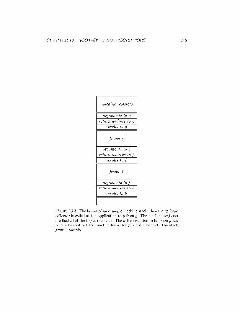
CHAPTER 13. ROOT{SET AND DESCRIPTORS 216
machine registers
arguments to p
return address to g
results to g
frame g
arguments to g
return address to f
results to f
frame f
arguments to f
return address to h
results to h
.
.
.
Figure 13.3: The layout of an example machine stack when the garbage
collector is called at the application to p from g. The machine registers
are ushed at the top of the stack. The call convention to function p has
been allocated but the function frame for p is not allocated. The stack
grows upwards.

CHAPTER 13. ROOT{SET AND DESCRIPTORS 217
fun g:
call p
frame descriptor for call to p
ret p:
fun f:
call g
frame descriptor for call to g
ret f :
Figure 13.4: Frame descriptors are inserted into the target code at the
addresses preceding the return addresses. Given the return address we
can �nd the frame descriptor. The vertical lines denote arbitrary code.
size of the call convention frame below the machine regis-
ters including return address and results.
register map describing arguments passed in machine regis-
ters. This is a one word bit vector (assuming 32 machine
registers).
The three arguments are uniquely determined at entry to a function. The
stack pointer points at the �rst cell above the machine registers. Given the
stack pointer and the three arguments, the garbage collector can determine
the argument part and the address of the top most function frame (g).
The garbage collector knows the number of machine registers on the target
machine. The garbage collector also knows the cell containing the return
address to function g (given the number of arguments).
The return address to function g is used to �nd the frame descriptor
for function g. The frame descriptor is stored in the program binary at the
addresses preceding the return address, see Figure 13.4.
Given the return address we can read the frame descriptor �elds in the
order: LiveCalleeSaveRegs, ushedCalleeSaveRegs, o�setToReturn, frame-
Size and frameMap. The �elds ushedCalleeSaveRegs and frameSize give
us the size of the function frame, including the call convention below the
function frame on the machine stack. We therefore know the address of the
next function frame on the machine stack. The �eld o�setToReturn gives us
the cell on the machine stack containing the return address where we �nd
the next frame descriptor.
Using the frame descriptors we can traverse the machine stack from top
to bottom. To calculate the liveAndFlushed sets, see Section 13.3, we need
to traverse the stack bottom up. This is done by reserving a single word

CHAPTER 13. ROOT{SET AND DESCRIPTORS 218
machine registers
arguments to p
return address to g
results to g
NULL
frame g
arguments to g
return address to f
results to f
addr. of frame desc.
g
frame f
arguments to f
return address to h
results to h
.
.
.
Figure 13.5: The address of the frame descriptor at the application to
function g, from f , is stored in the reserved word in the function frame
for f . We use NULL to denote the top most function frame. The stack
grows upwards.
in each function frame. On the way down the machine stack we store the
address of the frame descriptor of the preceding function frame, see Figure
13.5
On the way up the stack we calculate the liveAndFlushed set. Consider
Figure 13.5. At the function frame for f we know the frame descriptor for g.
Inside the function frame for g we �nd the address of the frame descriptor
for f which is used to calculate liveAndFlushed
f
.
13.6 Implementation
The frame descriptor, as presented, includes all information necessary for
callee save registers. However, we do not use callee save registers in the
initial implementation and we have therefore simpli�ed the descriptor. A
descriptor, in the implementation, contains a frame map and size of frame

CHAPTER 13. ROOT{SET AND DESCRIPTORS 219
plus call convention. Neither have we implemented the calculation of live
and ushed callee save registers. Currently, a single top down pass on the
machine stack is su�cient to calculate the root{set.

Part IV
Measurements
220

Chapter 14
Performance of the ML Kit
backend
We have divided the assessments in two chapters. In this chapter we focus
on the backend compiler. The garbage collector is tested in Chapter 15.
We still need to implement a few essential phases in the backend with the
register allocator being the most important. To test multiple argument pass-
ing we need a phase to un{curry functions and a phase to un{box records.
These de�ciencies make it uninteresting to compare our compiler with other
compilers and we refrain from doing so. However, we note that the compiler
compiles all of the Standard ML basis library and the test suite that comes
with the ML Kit.
1
One of the design goals was to implement a backend compiler organized
as a series of small phases which should make the compiler easier to compre-
hend and debug and at the same time not compromise compilation speed.
Implementing the backend has shown that this strategy indeed made the
task easier. The backend was implemented in a little more than two month
which includes adjustments to the runtime system.
2
Tagging, bit vector
calculations and the garbage collector algorithm was added in less than two
weeks. Section 14.1 gives an overview of the SML modules that implement
the new backend. To see the e�ect on compile times we compare our backed
with the backend of the ML Kit version 3 compiler (KitV3) in Section 14.3.
We investigate the e�ect of enabling tagging in Section 14.4. Tagging
has a negative e�ect on both execution times, memory usage and size of
binaries. We let tagging include boxing of lists, that is, if tagging is enabled,
then extra descriptors are inserted on boxed values and lists are represented
boxed [21].
1
Some modules (e.g., arrays and words) in the basis library do not compile with tagging
enabled because tagging of those modules has not yet been implemented in the runtime
system.
2
The runtime system is basically the same as in the ML Kit version 3.
221

CHAPTER 14. PERFORMANCE OF THE ML KIT BACKEND 222
Section 14.2 introduces the benchmark programs used in this chapter
and Chapter 15.
Compiler timings were measured on a Sun UltraSPARC 1 with 256Mb.
of main memory. Executables were run on a HP 9000/735 with 240Mb. of
main memory. The ML Kit is compiled using Standard ML of New Jersey,
version 110.0.3.
14.1 Files
The modules shown in Table 14.1 implement the new backend compiler in
the ML Kit. The garbage collector algorithm is implemented in module
GC.c (658 lines of C code) in the runtime system.
14.2 Benchmark Programs
All the benchmark programs compile without the Standard ML basis library
and are used to test both the backend compiler and garbage collector. We
use the following programs:
kitlife old: the game of life using lists. This version has not been optimized
for region inference.
kitlife35u: as kitlife old but optimized for region inference, that is, kitlife35u
uses less memory than kitlife old when compiled with region inference
enabled.
kitkb old: Knuth{Bendix completion. This version has not been optimized
for region inference.
kitkbjul1: as kitkb old but optimized for region inference.
kitkbjul9: as kitkbjul1 but more optimized for region inference, that is,
kitkbjul9 uses less memory than kitkbjul1.
kitsimple: A spherical uid{dynamics program. It performs a series of
oating point operations. It has not been optimized for region infer-
ence.
kitreynolds2: build a large balanced binary tree and search it. The pro-
gram performs well with region inference.
kitreynolds3: same as kitreynolds2 but uses lots of memory with region
inference.
kitqsort: an implementation of quick sort optimized for region inference.

CHAPTER 14. PERFORMANCE OF THE ML KIT BACKEND 223
SML Modules in the Backend Compiler
File Lines of code Notes
CALC OFFSET.sml 49
CalcOffset.sml 496 includes bit vector com-
putation.
CALL CONV.sml 54
CallConv.sml 292 implements the call con-
vention.
CLOS CONV ENV.sml 66
ClosConvEnv.sml 349 environment for closure
conversion.
CLOS EXP.sml 147
ClosExp.sml 2178 ClosExp language and
closure conversion algo-
rithm.
CODE GEN.sml 29
CodeGen.sml 2031 generates code for HP
PA{RISC.
FETCH AND FLUSH.sml 42
FetchAndFlush.sml 365 insert fetch and ush
statements.
LINE STMT.sml 191
LineStmt.sml 884 LineStmt language and
linearization algorithm.
REG ALLOC.sml 54
RegAlloc.sml 764 register allocation algo-
rithm.
SUBST AND SIMPLIFY.sml 50
SubstAndSimplify.sml 311 substitution and sim-
plify algorithm.
Total 8352
Table 14.1: The modules that implement the new backend compiler.
Signature �les are written with capital letters and functor �les with both
capital and small letters.

CHAPTER 14. PERFORMANCE OF THE ML KIT BACKEND 224
Benchmark Programs
Program Lines Of Code
kitlife old 205
kitlife35u 288
kitkb old 708
kitkbjul1 769
kitkbjul9 762
kitsimple 1115
kitreynolds2 91
kitreynolds3 92
kitqsort 157
kittmergesort 130
professor game 347
Table 14.2: Size of benchmark programs.
kittmergesort: an implementation of merge sort slightly optimized for re-
gion inference.
professor game: �nds all solutions to a 4 � 4 puzzle by searching the set
of possible solutions. This program has not been optimized for region
inference.
The size of the benchmark programs is shown in Table 14.2. We include
kitreynolds2 and kitreynolds3 in the test because they exhibit extreme be-
haviour with region inference.
14.3 Compilation Speed
Table 14.3 shows the compiler timings for our backend compiler. The ab-
breviations used are: closure conversion (CC), linearization (LS), dummy
register allocation (RA), fetch and ush (FF), calculate o�sets (CC), bit
vector calculation (CBV), simplify and substitution (SS) and code genera-
tion (CG).
Table 14.4 shows the compile timings for KitV3. The abbreviations used
are [22, 49, 50]: compile lambda (CL), copy propagation (CP), dead code
elimination (DE), register allocation (RA) and code generation (CG).
The closure conversion, linearization and fetch and ush phases are in-
cluded in the compile lambda phase in KitV3. In general it seems a little
more expensive to have three phases instead of one but we must keep in mind
that the compile lambda phase has been highly optimized. We have not done
any time pro�ling on the phases in our backend. Even in the case that we

CHAPTER 14. PERFORMANCE OF THE ML KIT BACKEND 225
Compilation Speed of New Backend
Program CC LS RA FF CO CBV SS CG Total
kitlife old 0.19 0.07 0.02 0.23 0.03 0.16 0.08 0.49 1.27
kitkbjul9 1.24 0.17 0.08 1.11 0.27 0.65 0.42 2.02 5.96
kitsimple 1.91 0.43 0.24 1.64 0.36 0.81 0.56 3.15 9.10
kitreynolds3 0.08 0.00 0.04 0.11 0.02 0.07 0.04 0.18 0.54
kitqsort 0.05 0.00 0.00 0.07 0.01 0.03 0.05 0.11 0.32
kittmergesort 0.08 0.00 0.02 0.09 0.05 0.05 0.03 0.15 0.47
professor game 0.28 0.12 0.03 0.34 0.04 0.25 0.11 0.62 1.79
Table 14.3: All timings are in seconds and do not include time used
on garbage collection. The register allocation phase (RA) is the dummy
register allocator as described in Chapter 5.
Compilation Speed of KitV3
Program CL CP DE RA CG Total
kitlife old 0.30 0.14 0.08 0.45 0.23 1.20
kitkbjul9 1.32 0.63 0.39 3.18 0.88 6.40
kitsimple 2.36 0.90 0.72 11.46 1.52 16.96
kitreynolds3 0.10 0.03 0.06 0.18 0.03 0.40
kitqsort 0.06 0.02 0.01 0.11 0.03 0.23
kittmergesort 0.07 0.02 0.01 0.17 0.05 0.32
professor game 0.32 0.10 0.10 1.32 0.25 2.09
Table 14.4: All timings are in seconds and do not include time used on
garbage collection.

CHAPTER 14. PERFORMANCE OF THE ML KIT BACKEND 226
cannot optimize either CC, LS or FF then we believe the time di�erence is
a small price for the simplicity gained in less complicated modules.
We cannot compare the timings for register allocation because we use
the dummy register allocator. However, we believe that we gain some time
on doing register allocation on the linearizated code instead of three address
code as is done in KitV3. We have a smaller number of nodes in the syntax
tree to process (e.g., records have not been compiled into three address
code instructions). The register allocator described in Chapter 5 performs
coalescing and we believe that it will not be necessary to use a separate copy
propagation phase.
We expect to incorporate dead code elimination into the phases where
it is easy to implement and a separate phase should not be necessary. For
instance, it is easy to remove code between a tail call and the next label.
We have to wait for the code produced by the register allocator described
in Chapter 5 but we do not expect to �nd code, without side e�ects, that
calculate and de�ne variables that are never used by the program.
We are surprised by the compile timings for our code generator being
higher than the timings for the code generator in KitV3 . Our code generator
should be as simple as the code generator in KitV3 and we probably have
a few time ine�ciencies that can be eliminated. Even though the code
generator generates code for allocation directives, records etc., then it is
basically driven by simple macro unfolding.
14.4 E�ect of Tagging
We have two important ine�ciencies when tagging is enabled. We add an
extra descriptor on boxed values which is expensive in both execution time
and memory usage. With tagging disabled it is possible to represent lists
unboxed [21]. Tagging e�ects execution time, memory usage and the size
of binaries. Table 14.5 shows the execution time and memory usage for
programs with tagging enabled and disabled. Memory usage is measured
in number of region pages requested from the operating system, that is, a
region page used in many regions during evaluation is counted as one region
page. The size of a region page is 1Kb. Timings are measured with the unix
program time. We report the best user time obtained after two or more
runs of the program.
We obtain considerable savings by disabling tagging in both execution
time and memory usage. Our results, especially on memory usage, with
tagging enabled are not as good as the results reported by Elsman [21]. We
believe it comes from the tagging of objects that are not seen by the poly-
morphic equality function. For instance, exception names, region vectors,
exception constructors, closures and shared closures are not tagged in the
experiments reported by Elsman.

CHAPTER 14. PERFORMANCE OF THE ML KIT BACKEND 227
E�ect of Tagging on Time and Memory Usage
Tagging Disabled Tagging Enabled
Program Time Memory Time Memory
kitlife old 41,18 7200 44,41(8%) 13110(82%)
kitlife35u 44,45 30 46,84(5%) 60(100%)
kitkb old 54,96 29250 65,04(18%) 46020(57%)
kitkbjul1 49,05 2550 58,39(19%) 4440(74%)
kitkbjul9 46,26 2010 55,26(19%) 3690(84%)
kitsimple 101,43 600 111,16(10%) 1260(110%)
kitreynolds3 25,98 16530 29,48(13%) 41490(151%)
kitreynolds2 10,88 30 11,05(2%) 30(0%)
kitqsort 11,74 5100 16,60(41%) 12750(150%)
kittmergesort 5,38 1200 7,77(44%) 3000(150%)
professor game 15,60 4170 18,41(18%) 9900(137%)
Table 14.5: All running times are in seconds. Memory usage is mea-
sured in number of region pages requested from the operating system.
One region page is 1Kb. The machine stack is not included. The over-
head
Tag�NoTag
NoTag
is written in percentages.
The size of binaries is shown in Table 14.6.
The results are mostly similar to the results reported by Elsman consid-
ering that our binaries are smaller. For instance, we report an overhead of
17% on kitsimple and Elsman reports an overhead of 10% where the size of
the binary for kitsimple with tagging enabled is 360Kb. and with tagging
disabled 328Kb.
The object �les are in general smaller in the new backend than in the old
backend. We believe it comes from more compact code generated and that
we use stub code when allocating into in�nite regions. In the old backend
we inline the code for allocating into an in�nite region. In the new backend
we jump to some stub code containing the code for allocating into an in�nite
region.

CHAPTER 14. PERFORMANCE OF THE ML KIT BACKEND 228
Size of Binaries
Tagging Disabled Tagging Enabled
Program Size of Binary Size of Binary
kitlife old 38553 51401(33%)
kitkbjul9 153425 184481(20%)
kitsimple 217697 254945(17%)
kitreynolds3 16209 19145(18%)
kitqsort 10737 13273(24%)
kittmergesort 13737 17177(25%)
professor game 58417 66953(15%)
Table 14.6: The size of binaries is in bytes. We show the size of the
stripped object �le. We have used the unix program gstrip. The over-
head
Tag�NoTag
NoTag
is written in percentages.

Chapter 15
Performance of the Garbage
Collector
In this chapter we present performance �gures for the garbage collector.
Section 15.1 measures the garbage collector combined with region infer-
ence. Section 15.1.3 compares the garbage collector with region inference in
the ML Kit and tries to answer the following question concerning the case
when region inference and garbage collection are combined: of the memory
that is reclaimed, what proportion is reclaimed by region management and
what proportion is reclaimed by the garbage collector? The heap size in u-
ences how often garbage collection is performed. We use di�erent heap sizes
in Section 15.2 and seek the optimal ratio of heap size to live data (i.e.,
0
).
Section 15.3 looks at the expense of inserting bit vectors into the binaries.
We focus on the cost of garbage collection and not the total cost of stor-
age management, that is, we do not investigate the cost of allocation and
region manipulation. Tarditi and Diwan [46] argue that it is necessary to
measure the total cost of storage menagement because the time used on
garbage collection may be less than the time used on other storage manage-
ment tasks. Actually, tagging, allocation and checking for garbage collection
seems as expensive as garbage collection and they report the total cost of
storage management in SML/NJ0.91 to be 19% to 46%; much higher than
the time used on garbage collection. Indeed it is interesting to perform
an analysis of the low{level details of the storage management scheme in
the ML Kit but such a comprehensive analysis is beyond the scope of this
project.
15.1 Cost of Garbage Collection
A popular garbage collection method used in Standard ML compilers is
generational garbage collection [3, 5]. Generational garbage collection is very
e�ective on Standard ML programs because they allocate a wast amount of
229

CHAPTER 15. PERFORMANCE OF THE GARBAGE COLLECTOR230
data with tiny life ranges and the wast majority of garbage is reclaimed in
the younger generations. The overhead of a well implemented generational
garbage collector on Standard ML programs is 5 to 10%. The overhead
depends on various parameters including the heap size contra the size of live
data. In an early version of SML/NJ an heap size of 7 times the amount of
live data gave an overhead of garbage collection of only 6% [3].
The garbage collector in the ML Kit cannot make use of the short life
range properties of Standard ML programs and must traverse all live data
at each garbage collection phase and not only regions containing newly al-
located data. However, region inference reclaims most short lived data at
almost no cost and it is therefore interesting to see how the combination of
simple copying garbage collection and region inference performs compared
to generational garbage collection. If region inference reclaims enough short
lived data such that the slower garbage collector is used at a frequency
corresponding to the frequency of garbage collecting the oldest generations
in a generational garbage collector then the performance may be almost
identical.
Many system parameters makes these simple judgements doubtful. For
instance, it is hard to estimate how region inference in uence on locality of
reference having the region heap represented as a linked list of region pages.
Also, our simple garbage collector uses a breadth �rst search to �nd live
data and not a depth �rst search (or an approximately depth-�rst search
[30, page 135]) which is better at obtaining good locality of reference. Our
garbage collector is also more complex in that in�nite regions are fragmented
and �nite regions are allocated on the machine stack. These complications
cost valuable time at garbage collection time.
We de�ne the overhead of garbage collection to be the time used on
garbage collection excluding time used on tagging, that is, the time used in
tracing and copying data. We time a program with tagging enabled (t
tag
)
and with both tagging and gc enabled (t
gc
). Time used on garbage collecting
is then t
gc
�t
tag
. Table 14.5 on page 227 shows our test programs with region
inference and tagging enabled. Garbage collection is disabled.
We measure memory usage as the number of region pages requested from
the operating system, that is, a region page can be used in many regions
during evaluation but is counted as one region page only. It is not in general
the case that all region pages are �lled with objects and we need the region
pro�ler [27] to measure the memory usage accurately. However, the region
pro�ler has not been ported to the new backend so counting region pages is
the best we can do. It is di�cult to estimate the inaccuracy that this incurs
on the results but we believe the general guidelines to hold. All timings
are measured with the unix program time. We report the best user time
obtained after two or more runs of the program.
The garbage collector is an initial implementation and contains several
ine�ciencies. We �nd it plausible that we can gain a speed up of 1.5 to 2 by

CHAPTER 15. PERFORMANCE OF THE GARBAGE COLLECTOR231
GC Enabled and RI Disabled
Program rp
total
rp
ts
t
gc
GC time # GC's
kitlife old 120 24 56.72 12.31(28%) 2833
kitlife35u 120 24 57.02 10.18(22%) 2833
kitkb old 5280 1747 236.60 171.56(264%) 675
kitkbjul9 390 91 114.19 58.93(107%) 3977
professor game 120 17 32.06 13.65(74%) 3201
Table 15.1: All timings are in seconds. Memory usage rp
ts
is the maxi-
mal number of region pages in to{space found after a garbage collection.
rp
total
is the number of region pages requested from the operating sys-
tem. Each region page is 1 Kb. The GC time is the di�erence t
gc
� t
tag
and the overhead
GCtime
t
tag
in percentages.
removind unnecessary debug code, unnecessary conditionals and optimizing
loops.
15.1.1 Simple Stop and Copy
In this section we measure the simple copying garbage collector without
region inference, that is, we let region inference use global regions only. All
values are allocated in global regions which is equivalent to turning region
inference o�.
We set
0
= 3:0 (see Section 11.8) and m = 120, where m is the smallest
amount of region pages that can be requested from the operating system
(i.e., when we call malloc). Table 15.1 shows the e�ect of enabling garbage
collection when region inference is disabled. The time used on garbage
collection GC time is calculated as the running time minus the time used
when both tagging and region inference are enabled (Table 14.5 on page
227). Using the time when region inference is enabled as base time may be
somewhat misleading. However, it has not been possible to �nd the base
time for all the programs when region inference was disabled because the
system ran out of memory. We belive the timings and overhead we report
in Table 15.1 to be a little (but not signi�cantly) higher than they should
be.
As expected, it is evident that a generational garbage collector with an
overhead of 5 to 10% is by far better than our simple stop and copy garbage
collector with region inference turned o�. Besides the lack of generations we
also have a more complicated heap split in region pages.
The optimized and unoptimized versions of kitlife behaves similarly but
there is a huge di�erence in the behavior of the two kitkb programs. We
believe the set of live values in kitkb old is so big that tracing and copying
are a major burden on the garbage collector. This is consistent with the

CHAPTER 15. PERFORMANCE OF THE GARBAGE COLLECTOR232
GC Enabled and RI Enabled
Program rp
total
rp
ts
t
gc
GC time # GC's
kitlife old 738 236 49.42 5.01(11%) 41
kitlife35u 90 28 50.38 3.54(8%) 3
kitkb old 12519 4163 73.50 8.46(13%) 21
kitkbjul1 1764 578 62.91 4.52(8%) 31
kitkbjul9 585 185 60.26 5.00(9%) 49
kitsimple 2067 679 125.10 13.94(13%) 6
kitreynolds2 30 3 12.75 1.70(15%) 1
kitreynolds3 30 7 32.81 3.33(11%) 2822
kitqsort 5994 1995 22.46 5.86(35%) 14
kittmergesort 4512 1494 9.24 1.47(19%) 7
professor game 149 40 19.56 1.15(6%) 149
Table 15.2: All timings are in seconds. Memory usage rp
ts
is the maxi-
mal number of region pages in to{space found after a garbage collection.
rp
total
is the number of region pages requested from the runtime system.
Each region page is 1 Kb. The GC time is the di�erence t
gc
� t
tag
and
the overhead
GCtime
t
tag
in percentages.
general experience that tuning a program for regions often makes them run
faster on a system that uses garbage collection and no region inference.
15.1.2 Region Inference plus Simple Stop and Copy
In this section we measure the performance of garbage collection when re-
gion inference is enabled and all regions are reclaimed each time a garbage
collection is initiated. We set
0
= 3.0 and m = 30.
In general we get much better timings with an overhead ranging from
6 to 35% and an average of 13%, see Table 15.2. Comparing the kitlife
and kitkb programs we see that the unoptimized versions use more time on
garbage collection but with a few percentages only. The kitqsort program
has a large overhead probably because the live set is big. The kitreynolds2
program is highly region inference optimized and we garbage collect one
time only.
1
The kitreynolds3 program, however, uses lots of memory with
an extremely small live set and the garbage collector is very e�ective. The
kitsimple, kittmergesort and professor game have not been region inference
optimized and they all perform well.
Comparing Table 15.1 and 15.2 we see that the size of to{space (i.e.,
rp
ts
) in general is bigger when region inference is enabled. We measure
number of region pages requested from the operating system. With the live
1
By construction, we always garbage collect at least one time.

CHAPTER 15. PERFORMANCE OF THE GARBAGE COLLECTOR233
objects allocated in many di�erent regions then we need more region pages
and each region page is less full. Because the to{space area increases then
the total memory usage rp
total
also increases. In general rp
total
should be
equal to rp
ts
0
.
Table 15.3 shows the memory usage obtained by enabling region infer-
ence, tagging and garbage collection. The results are interesting because we
have di�erent savings in the range from -276% to 100% where -276% means
that we use 276% more region pages when garbage collection is enabled.
We use more memory when enabling garbage collection on programs
that perform well without garbage collection. For instance, kitlife35u, kit-
simple and kittmergesort. First of all tagging is expensive and secondly the
garbage collector needs both a from{space and to{space. However, we get
amazing optimizations on other programs: kitlife old, kitkb old, kitkbjul9,
kitreynolds3 and the professor game. The only program that has been re-
gion inference optimized is kitkbjul9. The general guideline is that garbage
collection should not be enabled on programs that perform well on region
inference and enabling garbage collection may in fact have a negative ef-
fect. However, if you have a non region inference optimized program then
its likely that you save space by enabling the garbage collector.
Notice, that it is a guideline only and the e�ect of enabling garbage col-
lection very much depends on the program. For instance, we save memory,
using garbage collection, on a region optimized program as kitkbjul9. We
use more memory, using garbage collection, on kitqsort being region opti-
mized. We save memory, using garbage collection, on the professor game
not being region optimized. We use more memory, using garbage collection,
on kitsimple not being region optimized. Many factors (e.g., amount of
garbage generated, fragmentation in region pages, size of live set) in uence
the e�ect of enabling or disabling garbage collection.
15.1.3 Region Inference contra Garbage Collection
Experience has shown that region inference reclaims most of the garbage
generated but we do not have any measurements saying how much that
actually is. We have seen that the result of enabling garbage collection
very much depends on the target program and in general garbage collection
achieves good results on non region inference optimized programs. However,
can we estimate how much memory region inference recycles even on non
region inference optimized programs? We expect region inference to recycle
the vast amount of memory. We can do a simple estimation using Table
15.1 and 15.2, see Table 15.4.
We see that region inference gives us big savings on all programs both
in the number of times we perform garbage collection and the time we use
on garbage collection, hence region inference has a major impact on the
memory usage.

CHAPTER 15. PERFORMANCE OF THE GARBAGE COLLECTOR234
Memory Usage
Program RI GC RI TAG RI TAG�RI GC RI RI �RI GC
kitlife old 738 13110 12372(94%) 7200 6462(90%)
kitlife35u 90 60 -30(-50%) 30 -60(-200%)
kitkb old 12519 46020 33501(73%) 29250 16731(57%)
kitkbjul1 1764 4440 2676(60%) 2550 786(31%)
kitkbjul9 585 3690 3105(84%) 2010 1425(71%)
kitsimple 2067 1260 -807(-64%) 600 -1467(-244%)
kitreynolds2 30 30 0(0%) 30 0(0%)
kitreynolds3 30 41490 41460(100%) 16530 16500(100%)
kitqsort 5994 12750 6756(53%) 5100 -894(-18%)
kittmergesort 4512 3000 -1512(-50%) 1200 -3312(-276%)
professor game 149 9900 9751(98%) 4170 4021(96%)
Table 15.3: Memory usage RI GC is rp
total
when region inference and
garbage collection are enabled. RI TAG is rp
total
when region inference
and tagging are enabled. RI is rp
total
when region inference is enabled
and tagging/garbage collection disabled. The overheads
RI TAG�RI GC
RI TAG
and
RI�RI GC
RI
are in percentages.
Garbage Collection contra Region Inference
Program t
GC RI
t
GC NORI
# GC
GC RI
# GC
GC NORI
kitlife old 5.01 12.31 41 2833
kitlife35u 3.54 10.18 3 2833
kitkb old 8.46 171.56 21 675
kitkbjul9 5.00 58.93 49 3977
professor game 1.15 13.65 149 3201
Table 15.4: All timings are in seconds. t
GC RI
is the time used
on garbage collection when region inference is enabled and t
GC NORI
is when region inference is disabled. Likewise #GC
GC RI
is num-
ber of times we garbage collect when region inference is enabled and
#GC
GC NORI
is when region inference is disabled.

CHAPTER 15. PERFORMANCE OF THE GARBAGE COLLECTOR235
Memory Recycled by Region Inference
Program Approx. RI
kitlife old 94%
kitlife35u 99%
kitkb old 99%
kitkbjul1 99%
kitkbjul9 99%
kitsimple 99%
kitreynolds2 100%
kitreynolds3 31%
kitqsort 70%
kittmergesort 100%
professor game 98%
Table 15.5: We have approximated RI by calculating RI for each
garbage collection cycle and then report the average. We have
0
=
3.0 and m = 30.
With the garbage collector we can estimate the fraction of garbage re-
claimed by region inference. The fraction depends on the garbage collection
strategy used; eventually region inference reclaims all garbage (i.e., when
the program ends) and the fewer times we garbage collect the more data is
reclaimed by region inference. However, it is resonable to de�ne the data
reclaimed by garbage collection to be data that is reclaimed \too late" by
region inference corresponding to the chosen value of
0
. This fraction gives
a more precise indication of how eager region inference is.
Let g
i
be garbage collection phase i. Let L
i
be the amount of live data
after g
i
(i.e., size of to{space) and let A
p
be the total amount of data al-
located in the period between g
i
and g
i+1
. Let L
i+1
be the amount of live
data after g
i+1
and A
i+1
be the amount of allocated data before g
i+1
(i.e.,
size of from{space). The amount of data reclaimed by garbage collection
is A
i+1
� L
i+1
and the amount of data reclaimed by region inference is
L
i
+A
p
�A
i+1
. The total amount of data reclaimed is L
i
+A
p
� L
i+1
and
we get the fractions:
RI =
L
i
+A
p
�A
i+1
L
i
+A
p
� L
i+1
and GC =
A
i+1
� L
i+1
L
i
+A
p
� L
i+1
We did these calculations on the benchmark programs and Table 15.5
shows, in percentages, how much memory is approximately recycled by re-
gion inference.
The results are extraordinary but notice again, that memory is measured
in region pages. We believe this has a signi�cant and positive e�ect on RI

CHAPTER 15. PERFORMANCE OF THE GARBAGE COLLECTOR236
because every time a region is deallocated or reset then we count an entire
region page even though the region page is not full. However, even with
that inaccuracy we belive the results to be promising. Notice, that we only
measure the region heap, that is, we do not consider the values stored in
�nite regions which are also recycled automatically by region inference.
Figure 15.1 and 15.2 shows the two most interesting cases with GC (i.e.,
100-RI) as a function of time. Consider Figure 15.1. At garbage collection
number 5, the garbage collector reclaims a little less than 6% of the mem-
ory reclaimed since garbage collection number 4. Hence, region inference
reclaims more than 94% of the garbage in that period.
15.2 Heap Size
The garbage collection algorithm presented in Chapter 11 takes time pro-
portional to the number of live objects, that is, no time is used on reclaiming
garbage. We found the complexity to be t
C
= cU where U is the amount
of live data, and the constant c includes the time used to copy live objects,
update forward pointers, handling region status and the scan stack. We can
approximate the cost of garbage collection per object. Let H be the heap
size. The amount of garbage is then G = H � U and the cost per garbage
object is
cU
H � U
=
c
H=U � 1
Assuming the amount of live data U is approximately the same between
two garbage collections then the formula predicts that garbage collection
gets cheaper as the heap size increases.
Appel did a similar calculation with a simple copying garbage collector
and found the number of garbage collections and time used on garbage
collection to descrease as the heap size increased [2].
There are several issues in the ML Kit that may in uence the above
prediction.
1. garbage collection is combined with region inference and if region in-
ference reclaims most of the dead objects then the need for garbage
collection descreases.
2. for large heap sizes the live objects are likely to be scattered out on
the entire heap. As heap size increases we get more global pointers
which may have a signi�cant performance degradation on the virtual
memory system and cache performance. We get more page faults and
the cache is used less e�ciently.
3. The garbage collector must manage more region pages with a large
heap.

CHAPTER 15. PERFORMANCE OF THE GARBAGE COLLECTOR237
Memory Reclaimed by Garbage Collection
kitlife_old
0
1
2
3
4
5
6
7
8
1 4 7 10 13 16 19 22 25 28 31 34 37 40
GC no.
Rec
laim
ed b
y G
C (
%)
Figure 15.1: The �gure shows the amount of memory (in percentages)
reclaimed by garbage collection as a function of time. At garbage collec-
tion number 2, the garbage collector reclaims approximately 2% of the
memory reclaimed since garbage collection number 1. Hence region in-
ference reclaims 98% of the garbage in that period. Time is the garbage
collection cycle number.

CHAPTER 15. PERFORMANCE OF THE GARBAGE COLLECTOR238
Memory Reclaimed by Garbage Collection
kitqsort
0
5
10
15
20
25
30
35
40
45
50
1 2 3 4 5 6 7 8 9 10 11 12 13 14
GC no.
Rec
laim
ed b
y G
C (
%)
Figure 15.2: The �gure shows the amount of memory (in percentages)
reclaimed by garbage collection as a function of time. At garbage col-
lection number 10, the garbage collector reclaims approximately 7% of
the memory reclaimed since garbage collection number 9. Hence, region
inference reclaims 93% percent of the garbage in that period. Time is
the garbage collection cycle number.

CHAPTER 15. PERFORMANCE OF THE GARBAGE COLLECTOR239
Garbage Collection and Heap Size(
0
)
Program
0
rp
total
GC time #GC time=#GC rp
ts
kitkb old 2.2 9261 21.77 72 0.30 4196
kitkb old 2.5 10292 11.12 35 0.32 4105
kitkb old 3.0 12519 8.46 21 0.40 4163
kitkb old 3.5 13820 7.49 16 0.46 3940
kitkb old 5.0 18490 5.28 10 0.53 3692
kitsimple 2.2 1658 20.45 16 1.28 740
kitsimple 2.5 1722 16.05 9 1.78 677
kitsimple 3.0 2067 13.94 6 2.32 679
kitqsort 2.2 4463 34.87 67 0.52 2023
kitqsort 2.5 5087 13.23 28 0.47 2023
kitqsort 3.0 5994 5.86 14 0.42 1995
kitqsort 5.0 9975 2.04 6 0.34 1989
kittmergesort 2.2 4155 4.76 20 0.24 1875
kittmergesort 2.5 3765 2,79 12 0.23 1494
kittmergesort 3.0 4512 1.47 7 0.21 1494
Table 15.6: GC time is in seconds and is the time used on garbage
collection (i.e., t
gc
� t
tag
). Heap size (rp
total
) is the number of region
pages requested from the operating system. To{space (rp
ts
) is the largest
size of to{space after a garbage collection cycle measured in number of
region pages.
The heap size is controlled by the ratio
0
, see Section 11.8 on page 201. In
general we have h � l
0
, where h is the heap size and l is the amount of
live data. By increasing
0
we indirectly increase the heap size. We have
measured the benchmark programs with di�erent values of
0
.
All programs behaves similarly regarding the number of times we garbage
collect. As
0
increases the number of times we garbage collect decreases.
However, the total time used on garbage collection remains almost the same
for some programs: kitlife old, kitlife35u, kitkbjul1, kitkbjul9, kitreynolds2,
kitreynolds3 and the professor game. Table 15.6 shows the programs where
the time used on garbage collection decreases signi�cantly.
Why does the time on garbage collection not descrease as
0
increases
on all the programs? An important factor is that the programs not listed
in Table 15.6 are the programs with the smallest to{spaces (see Table 15.2).
This means that less time is used on each garbage collection cycle and the
total time used on garbage collection may not increase signi�cantly even
though we garbage collect more often.
Table 15.6 shows that the time used on each garbage collection cycle is

CHAPTER 15. PERFORMANCE OF THE GARBAGE COLLECTOR240
Code Size and Bit Vectors
Program
Size
(no gc.)
Size
(with gc.)
# FN # App
kitlife old 51401 57849(13%) 67 148
kitkbjul9 184481 207273(12%) 301 449
kitsimple 254945 290337(14%) 401 794
kitreynolds3 19145 22105(15%) 49 45
kitqsort 13273 14681(11%) 25 13
kittmergesort 17177 19049(11%) 31 26
professor game 66953 73937(10%) 107 98
Table 15.7: The table shows the size of stripped object �les with and
without garbage collection in bytes. The overhead comes from extra code
at entry to each function and the decriptors inserted at every application
point, see Chapter 13. The overhead
GC�NoGC
NoGC
is written in percentages.
The two last columns show the number of functions and the number of
non tail calls in the program.
either increasing, constant or descreasing depending on the program. We
would expect a constant behavior because the size of to{space is likely to
be independent of
0
. However, we see some variations in the to{space
column. An argument for an increasing time per garbage collection cycle
as
0
increases is that more time is spent manipulating region pages in
the garbage collector. We need more analyses in order to make further
conclusions.
We believe a value of
0
= 3.0 works well on most programs. How-
ever, some programs bene�t from adjusting
0
depending on the amount of
memory one wants to use.
15.3 Bit Vector Size
Table 15.7 shows the size of executables with and without garbage collection.
Tagging is enabled in both columns. We have measured the size of the object
�les, that is, the runtime system is not included in the sizes reported. The
object �les are stripped with the unix program gstrip.
The bit vectors used in the implementation have an overhead of one word
plus the words used to hold the frame map. The smallest bit vector is two
words. The code inserted at entry to each function is 12 words. The code
fetches a ag from memory and if the ag is set then the garbage collector
is called. Keeping the ag in a register would reduce the code to 9 words.
Given the number of functions and number of non tail calls we see that

CHAPTER 15. PERFORMANCE OF THE GARBAGE COLLECTOR241
most of the overhead comes from entry code to functions. For instance,
kitreynolds3 uses 2352 bytes on the entry code and 608 bytes on bit vectors.
This is a little more than 3 words per bit vector. Notice, that because all
variables are spilled the function frames are larger than they should be.
With the register allocator we expect to get a saving in memory used on bit
vectors. On kitsimple we use 19248 bytes on entry code and 16144 bytes on
bit vectors. This gives an average bit vector size of 5 words.
Allocating �nite regions in function frames increases the size of the frame
maps. The reason for kitsimple to use 5 words may be that many reals
are allocated in �nite regions and with tagging enabled each �nite region
containing a real has size 4 words. Extra space may also be used to keep
reals double aligned.

Chapter 16
Conclusion
In this chapter we discuss the contributions and some of the interesting
results obtained by combining region inference and garbage collection. We
then discuss future work.
16.1 Contributions
We have designed and implemented a new backend for the ML Kit. It has
been designed to be simple but still produce good quality code. Not having
a register allocator unfortunately makes it impossible for us to verify the
quality of the code.
The structure of the backend, with many small phases, has proven to
simplify the implementation greatly (i.e., the new backend separates aspects
of compilation which were intertwined in the old backend). Each phase
concentrates on a few minor tasks and is easier to implement and debug
than large and complicated phases that perform many tasks at the same
time. The succes of having many phases depends on the ability to express
the information computed in each phase in the intermediate languages. It
has been challenging to design the intermediate languages and we believe
we have succeeded; the LineStmt language is reused throughout the backend
and it incorporates all information computed in the di�erent phases. The
ability to de�ne polymorphic datatypes in Standard ML is a key feature in
the de�nition of LineStmt in the implementation. The backend has been
implemented in a little more than two months and already compiles the
Standard ML basis library.
The compilation speed of the new backend is faster than the old backend
on most of the benchmark programs. We believe, that this will also hold
after implementing the register allocator; the time used on register allocation
can be gained from optimizing some of the other phases including the code
generator.
We have developed a garbage collector that works with regions. We
242

CHAPTER 16. CONCLUSION 243
found that the region management scheme �ts well with a simple Cheyney
copying garbage collector where each in�nite region has its own scan pointer.
We solved the stop criteria problem using a scan stack of regions. Finite
regions gave us some problems, mainly because they are allocated on the
machine stack and therefore not copied. We solved the problems by marking
to{space and from{space region pages explicitly. The solution gave us a few
more tests when tracing objects but the garbage collector still performs well.
Tagging of values is implemented such that the same tags can be used
by the garbage collector and polymorphic equality function. We have seen
that tagging is very expensive, both in terms of space and time usage. The
size of object �les is also signi�cantly smaller when tagging is disabled. The
fact that using region inference without garbage collection requires no tags
is a signi�cant bene�t of the region management scheme.
We have implemented an e�cient root{set computation method based on
bit vectors inserted into the object �les. Object �les compiled with garbage
collection enabled are 10 to 15% larger than the corresponding object �les
without garbage collection. This is a resonable increase considering the
bene�ts, at runtime, of having bit vectors stored in the object �les.
We have seen dramatic e�ects of combining region inference and garbage
collection in Chapter 15. For instance, a program optimized for region in-
ference (e.g., kitkbjul9 contra kitkb old) may in fact give memory savings
with garbage collection, even if garbage collection is used without region
inference. However, region inference does reclaim the vast amount of mem-
ory. We have seen that the combination of region inference and garbage
collection performs well with an average execution time overhead of 13%
even though the garbage collector implementation has not been optimized.
The number of garbage collections (and time spent on garbage collec-
tion) descreases drastically for all programs if region inference is enabled.
This indicates that region inference does have the same e�ect as young gen-
erations in a generational garbage collector: a garbage collection cycle with
region inference enabled corresponds to a major garbage collection cycle in
a generational garbage collector.
Enabling region inference and garbage collection may have a negative
e�ect on memory usage compared to using garbage collection only. This is
mainly because of fragmentation problems, that is, many region pages are
almost empty. The fragmentation problem is a fundamental problem with
the region heap and it seems necessary to use both large and small region
pages to solve the problem.
A very positive result is that with the combination of garbage collection
and region inference, then the region management scheme reclaimes the vast
majority of the memory.
We have also seen that the number of garbage collections decreases as the
heap size increases (i.e., if
0
increases). We found that, for most programs,
0
= 3.0 is a resonable compromise between time spent garbage collecting
CHAPTER 16. CONCLUSION 244
and wasted space.
16.2 The ML Kit
The ML Kit is a research compiler that is freely available. The current
version is version 3 and can be found at
http://www.diku.dk/research-groups/topps/activities/mlkit.html
Version 3 does not include the new backend and garbage collector.
16.3 Future Work
It is important that we tune the implementation such that we can get more
information about the combination of region inference and simple copying
garbage collection. The register allocator and region pro�ler are two critical
components missing.
We have seen that fragmentation problems are essential for region in-
ference. Considering the increase in number of region pages used when
enabling region inference and garbage collection contra garbage collection
without region inference then there must be a lot of nearly empty region
pages. It seems plausible that a smaller region page size may solve some of
the fragmentation problems. However, it should be investigated if it is pos-
sible to implement a more exible system with two or more sizes of region
pages. Is it the case that the overall memory usage will bene�t from having
some regions use small region pages only and some regions use large region
pages only? Is it possible to improve memory performance using di�erent
sized region pages without compromising execution time?
To get more detailed information about the storage management system
in the ML Kit a comprehensive analysis looking at all aspects of storage
management is needed [46]. Detailed information about the time used on
manipulating regions, allocating into in�nite regions, tracing etc. may lead
to further optimisations. It is also possible to include the memory sub system
performance, that is, how paging and cache performance are in uenced by
region inference and the garbage collector [46, 20]. It is especially di�cult to
guess how the region heap in uences sub system performance as two region
pages allocated for the same region may be far apart in the address space.
Adding threading together with a graphics interface to the ML Kit would
make it possible to implement business like applications where the user
starts several threads running in di�erent windows. Threading in uences
garbage collection because garbage collection may only happen at gc{points,
see Chapter 13. Diwan et al. make sure that all threads reaches a gc{
point before they initiate garbage collection [19]. It is also interesting to
see if a database interface using methodologies from the world of functional

CHAPTER 16. CONCLUSION 245
programming can be designed and implemented. For instance, is it possible
to map, fold and apply a function on all or some of the entries in a table?

Bibliography
[1] Alfred V. Aho, Ravi Sethi, and Je�rey D. Ullman. Compilers, Princi-
ples, Techniques, and Tools. Addison Wesley, 1986.
[2] Andrew W. Appel. Garbage Collection Can Be Faster Than Stack
Allocation. Information Processing Letters, 25(4):275{279, 1987.
[3] Andrew W. Appel. Simple Generational Garbage Collection and Fast
Allocation. Software{Practice and Experience, 19(2):171{183, 1989.
[4] AndrewW. Appel. A runtime system. Lisp And Symbolic Computation,
3:343{380, 1990.
[5] Andrew W. Appel. Compiling With Continuations. Cambridge Univer-
sity Press, 1992.
[6] AndrewW. Appel.Modern compiler implementation in ML. Cambridge
University Press, 1998.
[7] Thomas H. Axford. Reference Counting of Cyclic Graphs for Functional
Programs. The Computer Journal, 33(5):466{470, 1990.
[8] Peter Bertelsen and Peter Sestoft. Experience with the ml kit and region
inference. Department of Mathematics and Physics Royal Veterinary
and Agricultural University, Copenhagen, Draft 1 of December 13 1995.
[9] Lars Birkedal. The ML Kit compiler { working note. Technical report,
DIKU, Department of Computer Science, University of Copenhagen,
July 1994.
[10] Lars Birkedal, Mads Tofte, and Magnus Vejlstrup. From region infer-
ence to von Neumann machines via region representation inference. In
Conference Record of the 23rd ACM SIGPLAN-SIGACT Symposium
on Principles of Programming Languages (POPL'96), pages 171{183,
St. Petersburg, Florida, January 1996. ACM Press.
[11] Daniel G. Bobrow. Managing Reentrant Structures Using Reference
Counts. ACM Transactions on Programming Lamguages and Systems,
2(3):269{273, July 1980.
246

BIBLIOGRAPHY 247
[12] David Callahan and Brian Koblenz. Register allocation via hierarchical
graph coloring. sigplan, 26(6):192{203, June 1991. pldi91.
[13] G. J. Chaitin. Register allocation and spilling via graph coloring. In
Proceedings of the SIGPLAN '82 Symposium on Compiler Construc-
tion, pages 85{94, June 1982.
[14] C. J. Cheney. A non-recursive list compacting algorithm. Communica-
tions of the ACM, 13(11):677{678, November 1970.
[15] Jacques Cohen and Alexandru Nicolau. Comparison of Compaction
Algorithms for Garbage Collection. ACM Transactions of Programming
Languages and Systems, 5(4):532{553, October 1983.
[16] George E. Collins. A Method for Overlapping and Erasure of Lists.
Communications of the ACM, 3(12):655{657, December 1960.
[17] Luis Damas and Robin Milner. Principal type-schemes for functional
programs. In Proceedings of the 9th Annual ACM Symposium on Prin-
ciples of Programming Languages, pages 207{212, January 1982.
[18] L. Peter Deutsch and Daniel G. Bobrow. An E�cient, Incremental, Au-
tomatic Garbage Collector. Communications of the ACM, 19(7):522{
526, 1976.
[19] Amer Diwan, Eliot Moss, and Richard Hudson. Compiler Support for
Garbage Collection in a Statically Typed Language. In Proceedings of
the SIGPLAN '92 Conference on Programming Language Design and
Implementation, pages 273{282. SIGPLAN, ACM Press, June 1992.
[20] Amer Diwan, David Tarditi, and Eliot Moss. Memory Subsystem Per-
formance of Programs Using Copying Garbage Collection. Technical
report, School of Computer Science, Carnegie Mellon University, De-
cember 1993. CMU-CS-93-210.
[21] Martin Elsman. Polymorphic Equality { No Tags Required. In Second
International Workshop on Types in Compilation, March 1998.
[22] Martin Elsman and Niels Hallenberg. An optimizing backend for the
ML Kit using a stack of regions. Student Project, Department of Com-
puter Science, University of Copenhagen (DIKU), July 5 1995.
[23] Robert R. Fenichel and Jerome C. Yochelson. A LISP Garbage{
Collector for Virtual{Memory Computer Systems. Communications
of the ACM, 12(11):611{612, November 1969.
[24] David A. Fisher. Bounded workspace garbage collection in an address{
order preserving list processing environment. Information Processing
Letters, 3(1):29{32, July 1974.

BIBLIOGRAPHY 248
[25] John P. Fitch and A. C. Norman. A note on compacting garbage col-
lection. Computer Journal, 21(1):31{34, February 1978.
[26] B. K. Haddon and W. M. Waite. A compaction procedure for variable{
length storage elements. Computer Journal, 10:162{165, August 1967.
[27] Niels Hallenberg. A Region Pro�ler for a Standard ML compiler based
on Region Inference. Student Project, Department of Computer Sci-
ence, University of Copenhagen (DIKU), June 14 1996.
[28] John L. Hennessy and David A. Patterson. Computer Architecture, A
Quantitative Approach. Morgan Kaufmann Publishers, second edition,
1996. ISBN: 1-55860-329-8.
[29] R. John M. Hughes. A semi{incremental garbage collection algorithm.
Software Practice and Experience, 12(11):1081{1082, November 1982.
[30] Richard Jones and Rafael Lins. Garbage Collection { Algorithms for
Automatic Dynamic Memory Management. John Wiley & SONS, 1997.
ISBN: 0-471-94148-4.
[31] H. B. M. Jonkers. A fast garbage compaction algorithm. Information
Processing Letters, 9(1):26{30, July 1979.
[32] Brian W. Kernighan and Dennis M. Ritchie. The C Programming Lan-
guage. Prentice Hall Software Series, second edition, 1988. ISBN: 0-13-
110362-8.
[33] P. J. Landin. The mechanical evaluation of expressions. Computer
Journal, 6(4):308{320, 1964.
[34] John McCarthy. Recursive Functions of Symbolic Expressions and
Their Computation by Machine, Part I. Communications of the ACM,
3:184{195, 1960.
[35] Robin Milner, Mads Tofte, and Robert Harper. The De�nition of Stan-
dard ML. MIT Press, 1990.
[36] Yasuhiko Minamide, Greg Morrisett, and Robert Harper. Typed Clo-
sure Conversion. In Conference Record of POPL '96: The 23
rd
ACM
SIGPLAN-SIGACT Symposium on Principles of Programming Lan-
guages, pages 271{283, St. Petersburg Beach, Florida, 21{24 January
1996.
[37] Steven S. Muchnick. Advanced Compiler Design and Implementation.
Morgan Kaufmann Publishers, San Francisco, California, 1997.

BIBLIOGRAPHY 249
[38] Tommy H�jfeld Olesen and Martin Koch. Compiling a Higher-Order
Call-by-Value Functional Programming Language to a RISC Using a
Stack of Regions. Master's thesis, Department of Computer Science,
University of Copenhagen, October 1996.
[39] Hewlett Packard. PA-RISC Assembly Language Reference Manual.
Hewlett Packard, fourth edition edition, January 1991.
[40] Hewlett Packard. PA-RISC Procedure Calling Conventions Reference
Manual. Hewlett Packard, second edition edition, January 1991.
[41] Hewlett Packard. PA-RISC 1.1 Architecture and Instruction Set Ref-
erence Manual. Hewlett Packard, third edition edition, February 1994.
[42] David A. Patterson and John L. Hennessy. Computer Organization &
Design, The Hardware/Software Interface. Morgan Kaufmann Publish-
ers, 1994. ISBN: 1-55860-281-X.
[43] Robert A. Saunders. The LISP System for the Q{32 Computer. In
Edmund C. Berkeley and G. Bobrow, editors, The Programming Lan-
guage LISP: Its Operation and Applications, pages 220{231. The M.I.T.
Press, fourth edition, March 1974. ISBN: 0 262 59004 2.
[44] Peter Sestoft. The garbage collector used in Caml Light. e-mail., Oc-
tober 1994.
[45] Laurent Sikl�ossy. Fast and read{only algorithms for traversing trees
without an auxiliary stack. Information Processing Letters, 1(4):149{
152, June 1992.
[46] David Tarditi and Amer Diwan. Measuring the Cost of Storage Manage-
ment. Technical report, School of Computer Science, Carnegie Mellon
University, May 1995. CMU-CS-94-201.
[47] Mads Tofte. Garbage Collection of Regions. This note outlines how
one can garbage collect regions, June 1997.
[48] Mads Tofte. A Brief Introduction to Regions. In Proceedings on the
1998 ACM International Symposium on Memory Management (ISMM
'98), pages 186{195, 1998.
[49] Mads Tofte, Lars Birkedal, Martin Elsman, Niels Hallenberg,
Tommy H�jfeld Olesen, Peter Sestoft, and Peter Bertelsen. Program-
ming with Regions in the ML Kit. Technical Report DIKU-report
97/12, Department of Computer Science, University of Copenhagen,
Universitetsparken 1, DK-2100 Copenhagen, April 1997.

BIBLIOGRAPHY 250
[50] Mads Tofte, Lars Birkedal, Martin Elsman, Niels Hallenberg,
Tommy H�jfeld Olesen, Peter Sestoft, and Peter Bertelsen. Pro-
gramming with regions in the ML Kit (for version 3). Techni-
cal Report DIKU-TR-98/25, Dept. of Computer Science, Univer-
sity of Copenhagen, 1998. (http://www.diku.dk/research-groups/
topps/activities/kit3/manual.ps).
[51] Mads Tofte and Jean-Pierre Talpin. A theory of stack allocation in poly-
morphically typed languages. Technical Report DIKU-report 93/15,
Department of Computer Science, University of Copenhagen, July 1993.
[52] Mads Tofte and Jean-Pierre Talpin. Implementing the call-by-value
lambda-calculus using a stack of regions. In Proceedings of the 21st
ACM SIGPLAN-SIGACT Symposium on Principles of Programming
Languages, pages 188{201. ACM Press, January 1994.
[53] Mads Tofte and Jean-Pierre Talpin. Region-based memory management
for the typed call-by-value lambda calculus. Submitted for publication,
April 1995.
[54] Omri Traub, Glenn Holloway, and Michael D. Smith. Quality and
Speed in Linear{scan Register Allocation. In Proceedings of the ACM
SIGPLAN 1998 Conference on Programming Language Design and Im-
plementation, June 1998.
[55] Magnus Vejlstrup. Multiplicity inference. Master's thesis, Department
of Computer Science, University of Copenhagen, September 1994. re-
port 94-9-1.
[56] Mitchell Wand and Paul Steckler. Selective and Lightweight Closure
Conversion. In Proceedings of the 21st ACM SIGPLAN-SIGACT Sym-
posium on Principles of Programming Languages, pages 435{445. ACM
Press, January 1994.
[57] Jim Welsh and John Elder. Introduction to Pascal. Prentice Hall In-
ternational, third edition, 1998. ISBN: 0-13-491549-6.
[58] Paul R. Wilson. Uniprocessor Garbage Collection Techniques, extended
remix { DRAFT. January 1994.
[59] David S. Wise and Daniel P. Friedman. The one{bit reference count.
BIT, 17(3):351{359, September 1977.