binary vs. non-binary constraints - department of computer ...fbacchus/papers/bcvwaij02.pdf ·...

Binary vs. Non-Binary Constraints�

Fahiem BacchusDepartment of Computer Science

University of TorontoToronto, Canada

[email protected]

Xinguang ChenDepartment of Computing Science

University of AlbertaAlberta, Canada

[email protected]

Peter van BeekDepartment of Computer Science

University of WaterlooOntario, Canada

[email protected]

Toby WalshDepartment of Computer Science

University of YorkYork, England

[email protected]

�This paper includes results that first appeared in [1, 4, 23]. This research has been supported in part by

the Canadian Government through their NSERC and IRIS programs, and by the EPSRC Advanced ResearchFellowship program.

1

Abstract

There are two well known transformations from non-binary constraints to bi-nary constraints applicable to constraint satisfaction problems (CSPs) with finitedomains: the dual transformation and the hidden (variable) transformation. Weperform a detailed formal comparison of these two transformations. Our com-parison focuses on two backtracking algorithms that maintain a local consistencyproperty at each node in their search tree: the forward checking and maintainingarc consistency algorithms. We first compare local consistency techniques suchas arc consistency in terms of their inferential power when they are applied to theoriginal (non-binary) formulation and to each of its binary transformations. Forexample, we prove that enforcing arc consistency on the original formulation isequivalent to enforcing it on the hidden transformation. We then extend these re-sults to the two backtracking algorithms. We are able to give either a theoreticalbound on how much one formulation is better than another, or examples that showsuch a bound does not exist. For example, we prove that the performance of theforward checking algorithm applied to the hidden transformation of a problem iswithin a polynomial bound of the performance of the same algorithm applied tothe dual transformation of the problem. Our results can be used to help decide ifapplying one of these transformations to all (or part) of a constraint satisfactionmodel would be beneficial.

2

1 Introduction

To model a problem as a constraint satisfaction problem (CSP), we specify a searchspace using a set of variables each of which can be assigned a value from some fi-nite domain of values. To specify the assignments that solve the problem, the modelincludes constraints that restrict the set of acceptable assignments. Each constraint isover some subset of the variables and imposes a restriction on the simultaneous val-ues these variables may take. In general, there are many possible ways of modeling aproblem as a CSP. Each model might contain a different set of variables, domains, andconstraints. The choice of model can have a large impact on the time it takes to find asolution [3, 17, 21], and various modeling techniques have been developed, includingadding redundant and symmetry-breaking constraints [9, 22, 25], adding hidden vari-ables [6, 24], aggregating or grouping variables together [3, 7], and transforming a CSPmodel into an equivalent representation over a different set of variables [7, 11, 19, 26].

One important modeling decision is the arity of the constraints used. Constraintscan be either binary over pairs of variables, or non-binary over three or more variables.Although a problem may be naturally modeled with non-binary constraints, these con-straints can be easily (and automatically) transformed into binary constraints. ManyCSP search algorithms are designed specifically for binary constraints, and further-more, like all modeling decisions, the choice of binary or non-binary constraints canhave a significant impact on the time it takes to solve the CSP.

In general, there is much research that remains to be done on the question of whichmodeling techniques one should choose when attacking a particular problem. In thispaper, we formally study the effectiveness of two modeling techniques that can be usedto transform a general (non-binary) CSP model into an equivalent binary CSP: the dualand hidden transformations [7, 19]. Our results give some guidance on the questionof choosing between binary and non-binary constraints. Further, the dual and hiddentransformations can be seen as extensions of the widely used techniques of aggregatingvariables together or adding hidden variables to reduce the arity of constraints and thusour results also provide information about these modeling techniques.

The choice of a CSP model also depends on the algorithm that will be used tosolve the model. We focus here on backtracking search algorithms that maintain alocal consistency property at each node in their search tree. Various types of localconsistency have been defined, and algorithms developed for enforcing them (e.g, [5,13, 14]). Algorithms that maintain a local consistency property during backtrackingsearch (e.g., [8, 10, 15, 16, 20]) can detect dead-ends sooner and thus have the potentialof significantly reducing the size of the tree they have to search. Such algorithmshave demonstrated significant empirical advantages and are the algorithms of choice inpractice. Hence, they are the most relevant objects of study.

We compare the performance of local consistency techniques and backtracking al-gorithms on three different models of a problem: the original formulation, the dualtransformation, and the hidden transformation. For the local consistency techniques,we establish whether a local consistency property on one model is stronger than orequivalent to a local consistency property on another. Among other results, we provethat arc consistency on the original formulation is equivalent to arc consistency on thehidden transformation, but that arc consistency on the dual transformation is stronger

3

than arc consistency on the original formulation. For backtracking algorithms, we giveeither a theoretical bound on how much better one model can be over another whenusing a given algorithm, or we give examples to show that no such polynomial boundexists. For example, we prove that the performance of an algorithm that maintainsarc consistency when applied to the original formulation is equal to its performancewhen applied to the hidden transformation. As another example, we also show that theperformance of the forward checking algorithm on the hidden transformation is nevermore than a polynomial factor worse than its performance on the dual, but that its per-formance on the dual can be an exponential factor worse than its performance on thehidden. Hence we have good theoretical reasons to prefer using the forward check-ing algorithm on the hidden transformation rather than on the dual transformation. Inthis way, our results can provide general guidelines as to which transformation, if any,should be applied to a non-binary CSP.

2 Background

In this section, we formally define constraint satisfaction problems and the dual andhidden transformations. In addition we briefly review local consistency techniques andthe search tree explored by backtracking algorithms.

2.1 Basic definitions

Definition 1 (Constraint Satisfaction Problem (CSP)) A constraint satisfaction prob-lem,

�, is a tuple �� whose components are defined below.

� = �� is a finite set of � variables.

� = �� !�"�#��$��%��& !�"��'�(� is a set of domains. Each variable �*)+� has acorresponding finite domain of possible values, ��& !�"�� .

= ��,-�%��(,/.0� is a set of 1 constraints. Each constraint ,2)3 is a pair��4�5�6(78�9,:�$��6<;�=��9,:�� defined as follows.

1. 4&5�6(7>�9,:� is an ordered subset of the variables, called the constraint scheme.The size of 4�5�6(78�9,:� is known as the arity of the constraint. A binaryconstraint has arity equal to 2; a non-binary constraint has arity greaterthan 2.

2. 6<;�=��9,:� is a set of tuples over 4�5�6$78�9,:� , called the constraint relation, thatspecifies the allowed combinations of values for the variables in 4�5�6(7>�9,:� .A tuple over an ordered set of variables ?A@B�%�C�%��D8� is an orderedlist of values ��E'��<E�D�� such that E�F-)3�>�� !�"��FG� , HI@KJ>��(L . A tupleover ? can also be viewed as a set of variable-value assignments ��-�NMEO�%��D:M2E�D8� .

4

Throughout the paper, we use � , � , 1 , and � to denote the number of variables,the size of the largest domain, the number of constraints, and the arity of the largestconstraint scheme in the CSP, respectively. As well, we assume throughout that for anyvariable � )!� , there is at least one constraint , )� such that � ) 4�5�6(7��9,:� .

Example 1 Propositional satisfiability (SAT) problems can be formulated as CSPs.Consider a SAT problem with � propositions, �C��<�� , and � clauses, (1) � �� , (2) �#�� , (3) �� and (4) �� . In one CSPrepresentation of this SAT problem, there is a variable for each proposition, � �� ,each variable has the domain of values ��O��J&� , and there is a constraint for each clause,,-�� , ,��>�"��%� , ,�>�"��>��&��%� and ,��>�"��>�� . Each constraintspecifies the value combinations that will make its corresponding clause true. Forexample, ,��8�"��<��%� , the constraint associated with the clause ��C�� , allowsall tuples over the variables �� , �� , and �� except the falsifying assignment ��O��'��J%� .

We use the notation 4�5�6(78�� to denote the set of variables a tuple � is over. If ? isany subset of 4�5�6(7>�� then �! ?#" is used to denote the tuple over ? that is obtained byrestricting � to the variables in ? . Given a constraint , and a subset of its variables$&% 4�5�6(78�9,:� , the projection ')(�, is a new constraint, where 4�5�6(78��'�(�,:� @ $

and6<;�= ��'�(�,:�C@ �*�! $ ",+��/) 6<;�=��9, �(� .

An assignment to a set of variables ? is simply a tuple over ? . An assignment � isconsistent if, for all constraints , such that 4�5�6(7>�9,:� % 4&5�6(7>�� , �! 4�5�6(7>�9, �-" ) 6<;�= �9,:� .A solution to a CSP is a consistent assignment to all of the variables in the CSP. If nosolution exists, the CSP is said to be insoluble.

Local consistency is an important concept in CSPs. Local consistencies are proper-ties of CSPs that are defined over “local” parts of the CSP, e.g., properties defined oversubsets of the variables and constraints of the CSP. Many local consistency propertieson CSPs have been defined (see [5] for a large collection).

Local consistency properties are generally neither necessary nor sufficient condi-tions for a CSP to be soluble. For example, it is quite possible for a CSP that is notarc consistent to have solutions, and for an arc consistent CSP to be insoluble. The im-portance of local consistency properties arise instead from the existence of (typicallypolynomial) algorithms for enforcing these properties.

We say that a local consistency property . can be enforced if there exists a (com-putable) function from CSPs to new CSPs, such that if

�is a CSP then . � � � is a

new CSP with the same set of solutions (and thus it must necessarily have the same setof variables).1 We call applying this function to a CSP enforcing the local consistency.Furthermore, we require that . � � � satisfy the property . , i.e., enforcing . mustyield a CSP satisfying .C , and that if

�satisfies . then . � � �C@ �

, i.e., enforcing alocal consistency on a CSP that already satisfies it does not change the CSP. The reasonfor enforcing a local consistency property is that often . � � � is easier to solve than

�.

In this paper we further restrict our attention to local consistency properties whoseenforcement involves only three types of transformations to the CSP: (1) the domains ofsome of the variables might be reduced, (2) some constraint relations might be reduced

1Note that we use the notation /�0 to denote the property of a problem 1 , and /�032 154 to denote theproblem resulting from enforcing the property /�0 .

5

(i.e., elements of 6<;�=��9,:� might be removed), and (3) some new constraints might beadded to the CSP.2 Note however, in all cases the variables of the CSP are unchangedand their domain of values can only be reduced.

A CSP is said to be empty if at least one of its variables has an empty domainor at least one of its constraints has an empty relation. An empty CSP is obviouslyinsoluble. Given a local consistency property . , we say that a CSP

�is not empty

after enforcing .C if . � � � is not empty.One of the most important local consistency properties is arc consistency [13, 14].

Definition 2 (Arc Consistency) Let� @ �� be a CSP. Given a constraint ,

and a variable � ) 4�5�6(78�9,:� , a value E )+�� !�� has a support in , if there is a tuple� ) 6<;�=��9,:� such that �! � " @ E . � is then called a support for �� M E'� in , . , is arcconsistent iff each value E of each variable �!) 4�5�6(78�9, � has a support in , . The entireCSP,

�, is arc consistent iff it has non-empty domains and each of its constraints is arc

consistent.

Arc consistency can be enforced on a CSP by repeatedly removing unsupportedvalues from the domains of its variables to create a subdomain.

Definition 3 (Subdomain) A subdomain � �of a CSP

� @ �� , is a set ofdomains, ��

��"�� , ��%��

��"��'�(� , where ��

��"��F � % �� !�"��FG� , for each

��F ) � . We say a subdomain is empty if it contains at least one empty domain. We saya subdomain � �

is arc consistent iff the CSP� � @ �� is arc consistent, where

� are the original constraints reduced so they contain only tuples over � �.3

Definition 4 (Arc Consistency Closure) An algorithm that enforces arc consistencycomputes the maximum arc consistent subdomain, and when applied to a CSP,

� @�� , it gives rise to a new arc consistent CSP called the arc consistency closureof�

, which we denote by 5��>� � � . We have that 5��8� � �-@ �� , where� ��

is the maximum arc consistent subdomain of�

, and �� are the originalconstraints reduced so that they contain only tuples over the subdomain � ��

.

Constraint satisfaction problems are often solved using backtracking search (for adetailed presentation see, for example, [12, 25]). A backtracking search may be seenas traversing a search tree. In this approach we identify tuples (assignments of valuesto variables) with nodes: the empty tuple is the root of the tree, the first level nodesare 1-tuples (an assignment of a value to a single variable), the second level nodesare 2-tuples (a first level assignment extended by selecting an unassigned variable,called the current variable, and assigning it a value from its domain), and so on. Wesay that a backtracking algorithm visits a node in the search tree if at some stage of the

2Only in Section 3.3 will we consider local consistency properties that might add new constraints.3According to Definition 1, the tuples of each constraint must only contain values that are in the domains

of the variables. A constraint can be reduced by deleting from the relation all tuples that contain a value �that was removed in the process of enforcing arc consistency. However, arc consistency algorithms do notnormally physically remove tuples from the constraint relations of 1 as this requires that the relations berepresented extensionally. Nevertheless, it is always implicit that the constraint relations are tuples over thereduced variable domains.

6

algorithm’s execution the algorithm tries to extend the tuple of assignments at the node.The nodes visited by a backtracking algorithm form a subset of all the nodes belongingto the search tree. We call this subset, together with the connecting edges, the searchtree visited by a backtracking algorithm.

The chronological backtracking algorithm (BT) is the starting point for all of themore sophisticated backtracking algorithms. BT checks a constraint only if all thevariables in its scheme have been instantiated. In contrast, the more widely used back-tracking algorithms enforce a local consistency property at each node visited in thebacktracking search. The consistency enforcement algorithm is applied to the inducedCSP. This is the original CSP reduced by the current assignment.

Definition 5 (Induced CSP) Given an assignment � of some of the variables of a CSP�, the CSP induced by � , denoted by

� + � , is the same as�

except that the domainof each variable � )B4�5�6(7>�� contains only one value �! � " , the value that has beenassigned to � by � , and the constraints are reduced so that they contain only tuples overthe reduced domains.

If the induced CSP is empty after enforcing the local consistency, the instantiationof the current variable cannot be extended to a solution and it should be uninstantiated;otherwise, the instantiation of the current variable is accepted and the search contin-ues to the next level. The forward checking algorithm (FC) [10, 15, 25] enforces arcconsistency only on the constraints which have exactly one uninstantiated variable. Bycomparison, on a problem that is not empty after enforcing arc consistency, the main-taining arc consistency or really-full lookahead algorithms [8, 16, 20], as their namessuggest, enforce full arc consistency on the induced CSP.

2.2 Dual and hidden transformations

The dual and hidden transformations are two general methods for converting a non-binary CSP into an equivalent binary CSP. The dual transformation comes from therelational database community and was introduced to the CSP community by Dechterand Pearl [7].

The hidden transformation, on the other hand, arose from the work of the philoso-pher Peirce. In particular, Rossi et al. [19] credit Peirce [18] with first showing that bi-nary relations have the same expressive power as non-binary relations. Peirce’s methodfor representing non-binary relations with a collection of binary relations forms thefoundation of the hidden transformation.

In the dual transformation, the constraints of the original formulation become vari-ables in the new representation. We refer to these variables, which represent the originalconstraints, as the dual variables, and the variables in the original CSP as the ordinaryvariables. The domain of each dual variable is exactly the set of tuples that are in theoriginal constraint relation. There is a binary constraint, called a dual constraint, be-tween two dual variables iff the two original constraints share some variables. A dualconstraint prohibits pairs of tuples that do not agree on the shared variables.

Definition 6 (Dual Transformation) Given a CSP� @ �� , its dual transfor-

mation ��'5�=�� = �� is defined as follows.

7

�� 2 � �� !4 � 2 � �� !4

� � 2 �� !4 � �*2 � �� 4��

� �

� �

��

� �

� �

� ��

Figure 1: The dual transformation of the CSP in Example 1.

� �� = � � � �� . � where � � �� . are called dual variables. For each

constraint ,-F of�

there is a unique corresponding dual variable � F . We use4�5�6(78� � FG� and 6<;�=�� F9� to denote the corresponding sets 4�5�6(7>�G, FG� and 6<;�=��9, F �(given that the context is not ambiguous).

� �� = �� !� � ��$��%�� !� � . �(� is the set of domains for the dual vari-

ables. For each dual variable � F , �� !� � FG�I@ 6<;�=��9,/F � , i.e., each value for � F is atuple over 4�5�6(7��9,-FG� . An assignment of a value � to a dual variable � F , � FIM � ,can thus be viewed as being a sequence of assignments to the ordinary variables�!) 4�5�6(78� � F9� where each such ordinary variable is assigned the value �! � " .

�� is a set of binary constraints over � �� called the dual constraints.

There is a dual constraint between dual variables � F and �� if$ @ 4�5�6(7>� � FG��

4�5�6(78� �� @�� . In this dual constraint a tuple ��F ) �� !� � FG� is compatible with atuple � � ) �� !� �� iff �F� $ "/@ � � $ " , i.e., the two tuples have the same valuesover their common variables.

It is important to note that in our definition all of the constraints of�

are converted todual variables, even the binary and unary constraints.

Example 2 In the dual transformation of the CSP given in Example 1, there are � dualvariables, � �%�� , one for each constraint in the original formulation as shown inFigure 1. For example, the dual variable � � corresponds to the non-binary constraint,-�� and the domain of � � contains all possible tuples except ��O��O��>� . Asan example of a dual constraint, the constraint between � � ( ,-��&��%� ) and � �( ,�>�"��%� ) requires that the first and second arguments of the tuples assigned to� � and � � agree. Hence, � � � M ��O��O��J%�$� is compatible with � � � M ��O��O��>�$� , but� � �-MA��O��O��J%�(� is incompatible with � � ��M ��O��J��>�(� .

In the hidden transformation, the set of variables consists of all the ordinary vari-ables in the original formulation with their original domains plus all the dual variablesas defined by the dual transformation. There is a binary constraint, called a hiddenconstraint, between a dual variable and each of the ordinary variables in the constraint

8

� � �� 2 � � � �� 4

� � �� 2 � � � �� 4

� � � �*2 �� 4

� � � �*2 � � �� 4

��

��

��

��

��

��

Figure 2: The hidden transformation of the CSP in Example 1.

represented by the dual variable. A hidden constraint enforces the condition that avalue of the ordinary variable must be the same as the value assigned to it by the tuplethat is the value of the dual variable.

Definition 7 (Hidden Transformation) Given a CSP� @ �� , its hidden trans-

formation�� ;�� = �� , � �� , �� is defined as follows.

�� = ��<�� . � , where �� is the original setof variables in � (called the ordinary variables) and � �%�� . are dual vari-ables generated from the constraints in . There is a unique dual variable � Fcorresponding to each constraint , F�) . When dealing with the hidden trans-formation, the dual variables are sometimes called hidden variables [6].

� �� = �� !�"��$��%�� !��'�(�� $��%��& !� � . �(� . For eachdual variable � F , �� !� � FG�C@ 6<;�=��9,/F � .

�� is a set of binary constraints over �� called the hidden con-straints. For each dual variable � , there is a hidden constraint between � andeach of the ordinary variables �!) 4�5�6(7�� . This constraint specifies that a tuple�/)+�� !� � � is compatible with a value E�)+�� !�"�� iff �! � "�@3E .

The hidden transformation has some special properties. The constraint graph of thehidden transformation is a bipartite graph, as ordinary variables are only constrainedwith dual variables, and vice versa, and the hidden constraints are one-way functionalconstraints, in which a tuple in the domain of a dual variable is compatible with at mostone value in the domain of the ordinary variable. The dual transformation can in factbe built from the hidden transformation by composing the hidden constraints between

9

the dual variables and the ordinary variables to obtain dual constraints between thedual variables, and then discarding the hidden constraints and ordinary variables [23].Note that we need not add hidden variables for binary constraints. However, as weobtain similar results if hidden variables are only introduced for ternary and higherarity constraints, we do not consider this further.

Example 3 In the hidden transformation of the CSP given in Example 1, there areJ*� variables ( � ordinary variables and � dual variables), as shown in Figure 2. Asan example of a hidden constraint, the constraint between � � ( ,-��&��%� ) and ��requires that the first argument of the tuple assigned to � � agrees with the value assignedto �#� . Hence, � � � M ��O��O��J��(� is compatible with ��:M �� , and � � � M ��O��O��J%�(� isincompatible with �� IM J&� .

In the following, we call a CSP instance�

the original formulation with respectto its dual transformation and hidden transformation. Because we usually deal withmore than one formulation of

�simultaneously, we use the notation �� , �� and

�� to denote the set of variables, the set of domains and the set of constraints in�

after it has been reformulated by some transformation � (to become a new CSP � � � � ).Also, we use ��& � �� "�� to denote the domain of variable � in � � � � .

3 Local Consistency Techniques

In this section, we compare the strength of arc consistency on the original formula-tion, and on the dual and hidden transformations. We show that arc consistency onthe original formulation and the hidden transformation are equivalent, but arc consis-tency on the dual transformation is stronger. We then compare several stronger localconsistency properties defined over the binary constraints in the dual and hidden for-mulations. We establish a hierarchy, with respect to a simple ordering relation, for thevarious combinations of local consistency and problem formulation.

Debruyne and Bessiere [5] compare local consistency properties defined on binaryCSPs. They define a local consistency property . �� to be stronger than another . ��( . �� . �� ) iff in any CSP instance in which . �� holds, then .C� holds, and. � to be strictly stronger than . �� ( . �� . �� ) if .C�� . �� and not. �� . � .

However, their definition of ordering among different local consistency propertiesdoes not provide sufficient discrimination for our purposes as we wish to simultane-ously compare changes in problem formulation and local consistency properties. Tothis end we define the following ordering relation.

Definition 8 Given two local consistency properties . �� and . �� , and two transfor-mations � and � for CSP problems (perhaps identity transformations), .C�� on � istighter than . �� on � , written . ��'��0�� . ��-� , iff

given any problem�

, if � � � � is not empty after enforcing . �� , then� � � � is also not empty after enforcing . �� .

10

. � on � is strictly tighter than .C�� on � , . �'�� . ��-� , iff . �'� �0��. � ��-� and not . � ��-� . � ��0� . And . � on � is equivalent to . � on � ,. �'��0� � . ��-� , iff . ��0� . ��-� and . ��-�� . �'� �0� . If the transfor-mations are identical; i.e., � @ � , then we simply write .C ��. �� .

The ordering relation we define is motivated by our desire to examine backtrackingsearch algorithms in which some form of local consistency is maintained during search.In such algorithms it is the occurrence of an empty subproblem at a node of the searchtree that justifies backtracking. Thus if . � is tighter than . � it follows (using thecontrapositive form of the definition: if

�is empty after enforcing . �� , then

�is also

empty after enforcing . �� ) that when an algorithm that maintains . �� backtracks ata node, then an algorithm that maintains . �� would backtrack at that node as well.

Debruyne and Bessiere’s ordering relation is defined by whether or not a problemsatisfies some local consistency property, whereas our ordering relation is defined bywhether or not a non-empty subproblem satisfies some local consistency property. Thisdistinction is important. For example, there exist problems for which the dual trans-formation is arc consistent but the original formulation is not, and problems wherethe original formulation is arc consistent while the dual is not. Thus, under Debruyneand Bessiere’s ordering (suitably modified to deal with two different problem formu-lations) arc consistency on these two formulations would be incomparable. Under ourordering relation, however, arc consistency on the dual transformation can be shownto be strictly tighter than arc consistency on the original formulation. As the followinglemma demonstrates, Debruyne and Bessiere’s ordering relation is stronger than ours.The relation �� is therefore unable to make as fine distinctions between differentlocal consistencies as the relation .

Lemma 1 . �� . �� implies . ��. �� .

Proof: Let�

be a problem which is not empty after enforcing . �� . Then there is anon-empty subdomain of

�in which . � holds and hence . � holds, since .C � � ��

. �� . Therefore�

is also not empty after enforcing .C�� , and . � �. �� .

Note also that .C�� . �� implies . �� .C�� , but not necessarily . �� . �� . In particular, . � �� . � failing to hold does not imply that . �� . �also fails to hold, as an ordering might exist between . �� and . �� even though no �� ordering exists.

3.1 Arc consistency on the hidden transformation

Consider a CSP�

with � variables, �� , each with domain ��O��J>� � � and con-straints given by, � �� , �� and �� . Figure 3shows the mappings between

�, its arc consistency closure 5��>� � � , its hidden trans-

formation� � ��;�� , and the arc consistency closure of its hidden transformation

5�� ;�� . It turns out that 5�� ;�� is the same as the hidden transfor-mation of the arc consistency closure

� � ��; � �<5��>� � �� . In this example, an ordinaryvariable has the same domain in 5�� and 5 �� ;��C� � �� and the domain of a dual

11

variable in 5�� ;�� is the same as the set of tuples in the corresponding con-straint that remain after enforcing arc consistency on the original formulation. We showin the following that these properties are true in general.

Lemma 2 If�

is arc consistent; i.e.,� @ 5�� , then

� � ��;�� is empty if and onlyif�

is empty.

Proof: If�

is empty then either it has an empty variable domain or an empty con-straint relation or both. In either of these cases

� � ��;�� will have an empty variabledomain. That is, for any

�, if

�is empty, then

� � ��;��C� � � is empty. (We do not needarc consistency for this direction.)

If� � ��;��C� � � is empty then we have one of two cases. (1)

� � ��; � � � � has an emptyvariable domain. In this case

�must also be empty. Otherwise, (2) there are no empty

variable domains but� � ��;�� has an empty constraint relation. We claim that case

(2) cannot occur if�

is arc consistent. Let ,�� be any of the hidden constraints,and say that it is a constraint between an ordinary variable � and a dual variable � .�� "�� is not empty so it must contain at least one value E . Furthermore, since

�is

arc consistent there must be a tuple � in �� such that the pair �"�� is a supportfor E in ,�� . That is, 6<;�= �9,�� (� must contain at least the pair �"�� . So none of theconstraints of

� � ��>;�� can be empty.

Theorem 1 Given a CSP�

,

1.�

is arc consistent if and only if� � ��;�� is arc consistent,

2.� � ��;��C�<5��>� � �� @ 5 �� ;��C� � �� , and

3. arc consistency on�

is equivalent to arc consistency on� � ��>;�� ; i.e., 5��

5��>� � � ��;�� .

Proof: (1) If the original formulation�

is not arc consistent, then there is at least onevalue E in the domain of an ordinary variable � and a constraint , such that � M E doesnot have a support in , . Hence, in

� � ��;�� , �+MAE will not have a support in thehidden constraint between the ordinary variable � and the corresponding dual variable� , and

� � ��;�� is not arc consistent either. On the other hand, suppose� � ��;��

is not arc consistent. Since by definition for every constraint , , 6<;�=��G,:� contains onlytuples whose values are in the product of the domains of 4�5�6(78�9,:� , each tuple in thedomain of a dual variable must have a support in a hidden constraint between the dualvariable and an ordinary variable. Hence, for

� � ��;�� not to be arc consistent theremust be a value E of an ordinary variable � and a dual variable � such that �� ME'� does not have a support in the hidden constraint between � and � ; thus �� ME'� cannot have a support in the corresponding original constraint , . Therefore, theoriginal formulation

�is not arc consistent either.

(2) First,� � ��; � � � � , � � ��;�� <5 �>� � �� , and 5��>� �� ;�� all have the same set of

variables (ordinary and dual) and the same constraint schemes since (a) enforcing arcconsistency does not alter the variables or the constraint schemes of a problem and (b)

12

� �� :

� ��

:

E � � � H �� @ � H �� E � � � �<�

�� 2 � � 4�� !"�� 2 ��!4�� $#�"�� 2 � 4�� !"�� 2 ��!4�� %"�� 2 �� 4�� !2�! � ! � #�4�"�� 2 � 4�� !2�! � # � %!4�"�� 2 � �!4�� !2�! � # � %!4�"

�� : ��

� � � � �� :

�$�� 2 � � 4�� ! � # � %"�$�� 2 � 4�� ! � # � %"�$�� 2 �� 4�� ! � # � %"�$�� 2 �� 4�� ! � # � %"

� �'& � )( ��+* �� & � �,( ��+* �� & � � ( � * � �

� �:

� :

� � � � �� $�� )� 2 � � 4��-��!"�$�� )� 2 � 4��-��!"

� � & � ( � � * � �� & � �,( ��+* �� & � �,( � * ��

� �� :

� �� :

�� :

�$�� )� 2 �� 4��-�$#�"�$�� )� 2 �� 4��-��%"

E � � � �

Achieving Arc Consistency Achieving Arc Consistency

�� :� �� :��.�� )� 2 � � 4�� ! � # � %"��.�� )� 2 � 4�� ! � # � %"��.�� )� 2 ��!4�� ! � # � %"��.�� )� 2 ��!4�� ! � # � %"

�!2�! � ! � #�4 � 2/# � ! � %!4 � 2�! � # � %!4�"��.�� )� 2 � � 4��

�

�!2�! � ! � #�4 � 2/# � ! � %!4 � 2�! � # � %!4�"�� )� 2 �� 4��

�!2�! � ! � #�4 � 2/# � ! � %!4 � 2�! � # � %!4�"��.�� )� 2 � � 4��

�� : ��

� H ��

Hidden Transformation

Hidden Transformation

Figure 3: An example to show the mappings between an original CSP, its hidden trans-formation, its arc consistency closure, the arc consistency closure of its hidden trans-formation, and the hidden transformation of its arc consistency closure.

13

the variables of the hidden are completely determined by the variables and the schemesof the constraints of the original problem.

Second, the set of domains of�� ;�� <5��>� � �� , � �� , is a subdomain of� � ��>;�� : enforcing 5�� on

�reduces the variable domains and the constraint rela-

tions, which simply has the effect, after applying the hidden transformation, of reducingthe domains of the ordinary and dual variables from their state in

� � ��;��C� � � . Further-more, by (1)

� � ��;�� <5��>� � �� must be arc consistent. Thus � �� is also asubdomain of 5��>� � � ��>;�� as � ��

� �� is the (unique) maximal arc consis-

tent subdomain of� � ��;�� . This means that for every variable � (ordinary or dual)

�� &� % ��

� �� &� .Third, we show for every variable � , ��

� �� &� % ��& �� &� ,

and hence that � �� @ � ��

. There are two cases to consider.(a) � is an ordinary variable. Since, 5�� ;��C� � �� is arc consistent, each value E )��

� �� &� must have a supporting tuple in every dual variable � that � isconstrained with. Furthermore, these supporting tuples must themselves have supportsin every ordinary variable that � is constrained with. In other words, E has a supportin each constraint by a tuple consisting of values from � ��

� �� . Thus the set of

domains of the ordinary variables in 5��>� � � ��;��C� � �� are an arc consistent subdomainof�

, and by maximality we must have that �� % �� &� .

Furthermore �� &�:@ �� &� by the construction of the hidden.

Thus for ordinary variables ��& �� &� % �>��

� �� &� . (b) � is adual variable. From (a) we know that every tuple � ) ��

� �� &� consistsof values of ordinary variables taken from � ��

. Hence, in 5�� , � will be inthe constraint relation of the constraint corresponding to � , and thus � will also be in��

� �� &� .Finally, in any hidden formulation the hidden constraints have the same intension.

Thus given that the variable domains � �� and � ��

are identi-cal all of the constraint relations (extensions) will be the same in

� � �>��;�� <5��>� � �� and5�� ;�� . (The constraint schemes are determined by the dual variables whichalso agree in these two formulations). Hence,

� � ��;�� <5 �� and 5 �� ;��C� � �<�have the same set of variables, domains for these variables, and constraints. That is,they are syntactically identical.

(3) Since 5��>� � � is arc consistent, 5�� is empty iff 5��>� � � ��>;�� is empty by(2) and Lemma 2.

Corollary 1 In any CSP�

, for each of the ordinary variables � in�

, �� "�� =��

� �� "�� = �� "�� .

Proof: The first equality follows from the construction of the hidden; the second fol-lows from (2) of Theorem 1.

3.2 Arc consistency on the dual transformation

We have proven that the original formulation is arc consistent if and only if its hiddentransformation is arc consistent. However, such an equivalence does not hold for thedual transformation.

14

Example 4 Consider a CSP�

with four Boolean variables and constraints:

,-��"��<�� @ �8��O��O��>�$��J��J��J%�(�>�,��"��<��%� @ �8��O��O��>�$��J��J��J%�(�>�,��"��<��%� @ �8��O��O��J%�$��J��J��>�(�>�

The original formulation�

is arc consistent. In its dual transformation, let the dualvariables � �%� � � , and � � correspond to the above constraints, respectively. Becauseneither of the tuples ��'��O��>� and ��J��J��J%� in the domain � � has a support in the dualconstraint between � � and � � , the domain of � � is empty after enforcing arc consistencyon the dual transformation. Thus � �'5�=�� is not arc consistent and 5��<� �'5�=� � �� isempty; i.e., 5�� 5 ��<� �'5�=9� .

Example 5 Consider a CSP�

with three Boolean variables and constraints:

,-��"��%� @ �8��J��J%�$�>�,��"��%� @ �8��J��J%�$�>�,��"��%� @ �8��J��J%�$�>�

The dual transformation � �'5�=�� is arc consistent. However, the original formulationis not arc consistent, because the value � for each of the variables will be removed fromits domain when enforcing arc consistency.

We can show that if the dual transformation is not empty after enforcing arc consis-tency, then the original formulation is not empty either after enforcing arc consistency;i.e., 5��<� �'5�=9�� 5�� . Together with Example 4 this shows that 5��<� ��5�=9�� 5�� .

Lemma 3 If a subdomain � �of a dual transformation � �'5�=�� is arc consistent,

then for each pair of dual variables � F and � � in � �'5�=� � � such that$ @ 4�5�6(7>� � FG� �

4�5�6(78� �� @ � , and for each �!) $ , '�� & �� FG� @ '��

�� .

Proof: For each � ) $and each tuple �+)&'�� &

� �� FG� there is a tuple �<F )

�� FG� such that �F � "!@ � . Because � �

is arc consistent, there must also bea tuple � � )2��&

�� such that �F� $ " @ � � $ " . Thus � @ �<F � " @ � � ��" . Be-

cause � ) ' � �� >�� , we have ' � ��

�� F � % ' � ��

�� . Similarly,

we can show that '�� % '��

�� FG� . Therefore, '��

�� FG� @

'�� .

From the arc consistency closure of � �'5�=� � �� , 5��<��'5�=� � �� , we can construct asubdomain for the original formulation

�(in Theorem 2 below we show that this sub-

domain is in fact an arc consistent subdomain of�

).

Definition 9 Let � �� denote the subdomain for the ordinary variables in

�that

is constructed from the domains for the dual variables in 5��<� �'5�=� � �<� as follows: foreach ordinary variable � in

�, choose a dual variable � in 5��>�<� �'5�=�� such that

15

� ) 4�5�6(7>� � � and set ��

�"�� to be ' � �� . Note that each

��

�"�� is well defined as (1) by our assumption that each variable is con-strained by at least one constraint, it is always possible to choose one such � , and (2)by Lemma 3, if there is more than one such � the result does not depend on the dualvariable we choose.

For example, the dual transformation of the CSP in Example 5 is arc consistent.Hence � ��

is ��>�� !� � �� @ �8��J��J��(�>�%�� %�C@ �8��J��J%�(�>�%�>�� C@ ��J��J%�(�� ,and � ��

is �� "��C@ �>J&�>�%�� "��%� @ �>J&�>�� "��%� @ �>J&�� .


, arc consistency on � �'5�=�� is strictly tighter than arcconsistency on

�; i.e., 5��<� �'5�=9�� 5�� .

Proof: We show that if 5��<� �'5�=� � �� is not empty, then neither is 5�� ; i.e. 5��>�<� ��5�=��5�� . Because the domain of each dual variable in 5��>�<��'5�=�� is not empty, its projec-tion over an ordinary variable cannot be empty either. So there is no empty domain

in � �� . In

�, for each ordinary variable � , each value E*) ��

�� "�� ,

and each constraint , , where � ) 4�5�6(78�G,:� , let E be the projection of the tuple � ofthe corresponding dual variable � . For each of the variables )B4�5�6(78�9, � , �! �"�)��

�� O� . Thus � is a support for �%� M E'� in constraint , , and furthermore

� is a tuple of values all of which come from � �� . Therefore, � ��

is anon-empty arc consistent subdomain of

�and thus 5��8� � � is not empty.

Example 4 shows that arc consistency on the dual transformation may be strictlytighter than arc consistency on the original formulation; i.e., 5�� B� �'5�=�<5��%� . There-fore, 5��<� ��5�=9�� 5�� .

By combining Theorem 1 and Theorem 2, we can make the following comparisonbetween arc consistency on the dual transformation and on the hidden transformation.

Corollary 2 Given a CSP�

, arc consistency on � �'5�=� � � is strictly tighter than arcconsistency on

� � ��>;�� ; i.e., 5��8�<� �'5�=�� 5��>� � � ��;�� .

3.3 Beyond arc consistency

Because the dual and hidden transformations are binary CSPs, we can enforce localconsistency properties that are defined only over binary constraints. Following [5], abinary CSP is ( H ,� )-consistent if it is not empty and any consistent assignment over Hvariables can be extended to a consistent assignment involving � additional variables.A CSP is arc consistent (AC) if it is ( J , J )-consistent. A CSP is path consistent (PC) ifit is (

�, J )-consistent. A CSP is strongly path consistent (SPC) if it is ( H , J )-consistent

for each J�� H�� . A CSP is path inverse consistent (PIC) if it is ( J , � )-consistent. ACSP is neighborhood inverse consistent (NIC) if any instantiation of a single variable� can be extended to a consistent assignment over all the variables that are constrainedwith � , called the neighborhood of � . A CSP is restricted path consistent (RPC) if itis arc consistent and whenever there is a value of a variable that is consistent with justone value of an adjoining variable, every other variable has a value that is compatible

16

with this pair of values. A CSP is singleton arc consistent (SAC) if it is not empty, andthe CSP induced by any instantiation of a single variable is not empty after enforcingarc consistency.

Debruyne and Bessiere [5] demonstrated that, SPC �� SAC � �� PIC � �� RPC� �� AC, and NIC �� PIC, where “ �� ” is the ordering relation defined in theirpaper, as discussed in Section 3. Thus, by Lemma 1 we immediately have that SPC SAC PIC RPC AC, and NIC PIC.


, neighborhood inverse consistency on� � ��>;�� is equiv-

alent to arc consistency on�� ;�� ; i.e., � � �� ;�� 5�� >;�� .

Proof: Since � � � A5�� , we immediately have � � �� >��;�� A5�� ;�� . Con-versely, suppose 5�� ;�� is not empty. For a dual variable � , its neighborhoodin 5�� >��;��C� � �� is 4�5�6(7>� � � . Thus an instantiation of � with a tuple � from its do-main in 5�� ;��C� � �� can be extended to a consistent assignment of its neighboringvariables, where for each of the ordinary variables � ) 4&5�6(7>� � � , � is instantiated with�! � " ( �! ��" must be in the domain of � because it is the only support for � in the hiddenconstraint between � and � ). For an ordinary variable � , � only has constraints withdual variables. An instantiation of � with a value E from its domain in 5�� ;��C� � ��can be extended to a consistent assignment including all its neighborhood, where foreach of the dual variables � in its neighborhood, � is instantiated with a tuple � such that�! � "#@ E (also, such a tuple must exist because �� M E'� has at least one support in thehidden constraint between � and � ). Therefore, the hidden transformation is not emptyafter enforcing neighborhood inverse consistency; i.e., � � �� ;�� is not empty.In fact, 5�� ;�� is already neighborhood inverse consistent.

Because neighborhood inverse consistency on the hidden transformation collapsesdown onto arc consistency those consistencies that are weaker than neighborhood in-verse consistency but tighter than arc consistency, e.g., path inverse consistency and re-stricted path consistency, are also equivalent to arc consistency. That is, � � �� ; �� >� � � ��;�� 6 � �� ;�� 5�� ;�� (and by the equivalence 5�� ;�� 5��established in Theorem 1, each of these local consistencies on the hidden transforma-tion is in turn also equivalent to arc consistency on the original formulation).

However, neighborhood inverse consistency on the dual transformation does notcollapse. It is strictly tighter than arc consistency. In fact, the even weaker restrictedpath consistency is strictly tighter than arc consistency on the dual.

Example 6 Consider a CSP with three Boolean variables and constraints:

,-��"��%��%� @ �8��O��>�$��J>��J%�(�>�,�8�"��&��%� @ �8��O��>�$��J>��J%�(�>�,�8�"��%��%� @ �8��O��J%�$��J>��>�(�>�

The dual transformation of this problem is arc consistent but not restricted path con-sistent (RPC). Furthermore, enforcing RPC on the dual transformation yields an emptyCSP. Thus we have that 6 � ��<� �'5�=9�� 5��<� �'5�=�� ; i.e., 6 � � is strictly tighter on the dual.

17

Along with the previous orderings this immediately gives that both � � �>�<� �'5�=�� 5��(� �'5�=9� , and � � ��<� ��5�=9�� 5��>�<� ��5�=�� .

Although neighborhood inverse consistency and path inverse consistency on thehidden transformation do not provide any additional power over arc consistency, thesame is not true for singleton arc consistency.

Example 7 Consider a CSP with three parity constraints: even( �C� � �� ), even( � � �� ), and even( � � � �� ). If �#� is set to 1, and the other variables have domain��O��J&� then the hidden transformation is arc consistent but not singleton arc consis-tent. Furthermore, enforcing singleton arc consistency on this problem yields an emptyCSP. Thus we have 7�5��>� � � �>��;�� A5��>� � � ��;�� and 7�5�� ;�� >��;�� (since � � �� ;�� 5�� ;�� ).


, singleton arc consistency on � �'5�=� � � is tighter than sin-gleton arc consistency on

� � �>��;�� ; i.e., 7�5��<� �'5�=9�� 7�5�� ;�� .

Proof: First we define a function � from the arc consistent subdomains of � �'5�=�� to subdomains of

� � ��; � � � � . Let � be an arc consistent subdomain of � �'5�=�� . In�#� � � each dual variable � will have the same domain as it did in � , ��&

�� @

�� , and the domain of each ordinary variable � , ��

� �"�� , is set to beequal to '�� &

�� for some dual variable � such that � ) 4�5�6(7>� � � . � is well

defined, as from Lemma 3 we know that since � is an arc consistent subdomain of� �'5&=�� , ��

� �"�� is independent of which dual variable � we choose to project.� has three relevant properties. (1) �#� �N� is an arc consistent subdomain of

� � ��;�� .For each ordinary variable � we have that ��

� �"��/@ '�� for every dual

variable � that � is constrained with. Thus, every value of � has a support in each ofthe dual variables it is constrained with (take one of the tuples whose projection wasthat value), and every tuple � of every dual variable � has a support in each of the or-dinary variables it is constrained with (take the projection of � on that variable). (2)If � �

is a subdomain of � , then �#� � � � is a subdomain of �#� �N� . This is obvious fromthe definition of � . (3) �#� �N� is an empty subdomain, if and only if � is an emptysubdomain.4 The only non-trivial case is when �#� � � contains an empty domain for anordinary variable � . But in that case there must be a dual variable � with � )*4&5�6(7>� � �such that ' � �� &

�� C@ � . And this can only be the case if ��

�� is itself empty;

i.e., � contains an empty domain.Now we show that if 7�5��<� ��5�=�� is not empty then neither is 7�5��>� � � ��;�� <� ;

i.e., 7�5��<� �'5�=G�� 7�5�� >;�� . Let �� @3� � �� and ��N@��#� �� . Our claimis that �� is a non-empty singleton arc consistent subdomain of

� � ��;�� .First, since 7�5��<��'5�=� � �� is arc consistent and non-empty, � � �� @ ��

is an arc consistent and non-empty subdomain of � �'5�=�� . Thus, �� is a non-emptymember of the domain of the function � and by (3) ��N@�#� �� is non-empty and weneed only prove that it is singleton arc consistent.

Let � be a dual variable, and � a tuple in �� . We must show that ��+ �� (i.e.,

�� in which �� has been reduced to the singleton �*�(� ) contains a non-empty

4By Definition 3 a subdomain is empty if it contains an empty domain for some variable.

18

arc consistent subdomain. However, since � � is singleton arc consistent, � ��+ �� con-tains a non-empty arc consistent subdomain 5�� + �� . �#�<5��8� � � + �� is easily seento be a subdomain of � ��+ �� , and thus by (1) and (3) �#�<5��8� � �3+ �� must be a non-empty arc consistent subdomain of � ��+ �� . On the other hand, let � be an ordinaryvariable and E a value in its domain. To show that � ��+ � � contains a non-emptyarc consistent subdomain, we choose any dual variable � that � is constrained with,and a tuple � from the domain of � such that � � " @BE . Now if we consider ��+ �� and its non-empty arc consistent subdomain 5�� + �� , we can similarly show that�#�<5 �>� ��+ �� is a non-empty arc consistent subdomain of � ��+ � � .

In the hidden transformation, for each pair of dual variables � F and �� , where4�5�6(78� � FG�� 4�5�6(78� �� @ � , enforcing strong path consistency adds a constraint between� F and �� . This constraint ensures that a tuple from � F agrees with a tuple from � �on the shared ordinary variables. The constraint is identical to the dual constraint be-tween � F and �� in the dual transformation. Thus, strong path consistency on the hiddentransformation must be as strong as on the dual. In fact, we can show their equivalence.


, strong path consistency on� � ��;�� is equivalent to

strong path consistency on � �'5�=�� ; i.e., 7 � �� >��;�� 7 � ��(� �'5�=9� .Proof: See [4].

Figure 4 summarizes our results. If there is a directed path between consistencyproperties � and � , then � is tighter than � . If the path contains a strictly tighterthan link then � is strictly tighter than � . Note that some of the relationships betweenconsistency properties are not completely characterized. For example, it is an openquestion whether or not 7�5�� ;�� 7�5��>�<� �'5�=�� .

4 Backtracking Algorithms

In this section, we compare the performance of three backtracking algorithms—thechronological backtracking algorithm, the forward checking algorithm, and the main-taining (generalized) arc consistency algorithm—when solving the original formulationand the dual and hidden transformations of a problem. Our results are proven under theassumption that a backtracking algorithm finds all solutions to a problem.

Given two backtracking algorithms and two formulations of a problem we identifywhether or not the relation “one combination can be only polynomially worse than an-other combination” holds. To formalize this relation we must first specify quantitativemeasures of the size of a CSP and the cost of solving a CSP using a given algorithm.

We denote by �� the size of a CSP�

. Consistent with real-world practice,we assume that the domains of the variables are represented extensionally and that theconstraints are represented intensionally. Thus, to specify the variables, domains, andconstraints of a (possibly transformed) CSP

�takes �N�"� � �)�� 1 �&� space, where

� denotes the number of variables, � the size of the largest domain, 1 the number ofconstraints, and � the arity of the largest constraint scheme in

�. Since the dual and

the hidden are transformations of an original (non-binary) formulation�

, we can also

19

sac(dual) pic(dual) rpc(dual) ac(dual)spc(dual)

spc(hidden) sac(hidden) pic(hidden) rpc(hidden) ac(hidden)

ac

nic(dual)

nic(hidden)

Figure 4: The hierarchy of relations between consistencies on the original, dual, andhidden formulations. A bi-directional arrow is equivalence, � , a double headed arrowis the strictly tighter relation, � , and an ordinary arrow is the tighter relation, .

20

specify their sizes in terms of the parameters of�

. In particular, let � , � , 1 , and � bethe parameters of an original (non-binary) formulation

�. In the worst case, the trans-

formation ��'5�=�� takes �N��1 �!1 �� !1 � � space and the transformation� � ��;��

takes �N�<�"� � 1 � � �"�� 1 �� 1 �&� space. Thus, the dual and hidden transfor-mations can require space that grows exponentially with the arity of the constraints inthe original formulation. In practice, one would certainly want to limit the arity of theconstraints to which these transformations are applied.

To solve a CSP with a backtracking algorithm, one must specify the variable or-dering the algorithm uses to determine which variable to instantiate next. It is wellknown that the variable ordering used can have an exponential effect on the cost ofsolving a CSP. Thus an exponentially difference in performance between two algo-rithm/formulation pairs is always trivially possible under particular variable orderings.Hence, to formalize a sensible notion of “only polynomially worse” we must do so ina way that is independent of any particular variable ordering. In our definitions weachieve this independence by quantifying over all possible orderings.

Formally, we define a variable ordering function � to be a mapping from a tuple �(a node making a, possibly empty, set of variable-value assignments) and a CSP

�to

a new variable not in 4�5�6$7>�� . We say that a variable ordering � is an ordering for aproblem

�if it is defined over the variables of

�. In addition, we say that an algorithm�

uses the variable ordering � if � characterizes the choices made by�

at the variousnodes

�visits as it does its backtracking search; i.e.,

�next instantiates the variable �

when it is at node � if and only if � �"��C@ � .We denote by �� the cost of solving a CSP

�using an algorithm

�and

a variable ordering � . This cost is determined by the number of nodes visited by thealgorithm and the cost at each node. In turn, the cost at each node is determined bythe cost of enforcing the local consistency property maintained by the backtrackingalgorithm and the cost, if any, of determining the next variable to instantiate (the costof the function � � .

Definition 10 Let�

- � denote algorithm�

applied to problems transformed by a trans-formation � . Given two backtracking algorithms

�and (possibly identical), and two

transformations � and � for CSP problems (perhaps identity transformations),

1.�

- � can be only polynomially worse than - � , written�

- �� - � , iff givenany CSP

�and variable ordering �� for � � � � , there is a variable ordering �� for

� � � � such that,

�� $� �� $� �� polynomial function of � � � � �� $� �� :� � ��$�

That is, the cost of solving � � � � using�

and �� is at most a polynomial factorworse than the cost of solving � � � � using and �� .

2.�

- � can be superpolynomially worse than - � , written�

- � �� - � , iff�

- � �� - � (i.e., the negation of polynomially worse), iff there exists a CSP�

and a variable ordering �� for � � � � , such that for any variable ordering �� for

21

� � � � ,�� $� �� :� � �$� ��

� superpolynomial function of � � � � �� $� �� $�

That is, the cost of solving � � � � using�

and �� is at least a superpolynomialfactor worse than the cost of solving � � � � using and �� .

To prove a relationship�

- � � �� - � , we (1) establish that the number of nodesvisited by

�on � is at most a polynomial factor more than the number of nodes visited

by on � , (2) establish that the time complexity of enforcing the local consistencyproperty maintained by

�at each node is at most a polynomial factor worse than the

time complexity of enforcing the local consistency property maintained by at eachnode, and (3) establish that the time complexity of � � is at most a polynomial factorworse than the time complexity of �� . In turn, to prove condition (1), we establisha correspondence between the nodes in the ordered search tree generated by � � thatare visited by

�and the nodes in the ordered search tree generated by � � that are

visited by . In the definition of�

- � � �� - � , the existential (there is a variableordering � � ) occurs within the scope of two universal quantifiers (any CSP

�and any

variable ordering � � ) and thus � � can depend on both�

and �� . To prove condition(3), we show how to construct �� given only polynomial access to � � and polynomialadditional computation.

4.1 Discussion

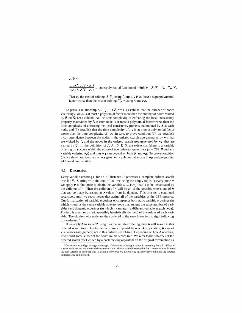
Every variable ordering � for a CSP instance�

generates a complete ordered searchtree for

�. Starting with the root of the tree being the empty tuple, at every node �

we apply � to that node to obtain the variable � @ � �"� � that is to be instantiated bythe children of � . Then the children of � will be all of the possible extensions of �that can be made by assigning � values from its domain. This process is continuedrecursively until we reach nodes that assign all of the variables of the CSP instance.Our formalization of variable orderings encompasses both static variable orderings (inwhich � returns the same variable at every node that assigns the same number of vari-ables) and dynamic orderings (in which � can return a different variable at each node).Further, it assumes a static (possibly heuristically derived) of the values of each vari-able. The children of a node are thus ordered in the search tree left to right followingthis ordering.5

If we apply�

to solve�

using � as the variable ordering, then�

will search in thisordered search tree. Due to the constraints imposed by � on

�’s operation,

�cannot

visit a node (assignment) not in this ordered search tree. Depending on how�

operates,it will visit some subset of the nodes in this search tree. We refer to the sub-tree (of theordered search tree) visited by a backtracking algorithm on the original formulation as

5Our results would go through unchanged if the value ordering is dynamic assuming that all children ofa given node are instantiations of the same variable. All that would be needed is for � to return in addition tothe next variable an ordering over its domain. However, we avoid doing this since it would make the notationunnecessarily complicated.

22

231231

321321

3121

1

321

}),({,}),({

}),({,}),({

})({,})({

({})

1,...,3},{)(

},,{

xbxaxxaxbx

xbxaxxaxax

xbxxax

x

ibaxdom

xxxVars

CSP P

i

======

======

====

=

==

=

νν

νν

νν

ν 1 ax = 1bx =

2 ax = 2 bx = 3 ax = 3 bx =

3 ax = 3 bx = 3 ax = 3 bx = 2 ax = 2 bx = 2 ax = 2 bx =

Figure 5: The ordered search tree generated by a variable ordering.

the original search tree, the sub-tree visited when solving the dual transformation asthe dual search tree, and the one visited when solving the hidden transformation as thehidden search tree. All of these sub-trees are defined with respect to particular variableorderings (each of which generates a particular ordered search tree). Figure 5 shows anexample of a CSP instance

�, variable ordering � for

�, and the complete search tree

generated by � .As we have defined them, a variable ordering can play either a descriptive or a

prescriptive role. Say that we run�

on � � � � and we use some heuristic function tocompute the next variable to instantiate at every node of the search tree. This heuristicfunction could use various pieces of the state of the program in computing its answer.For example, in an algorithm like FC, the minimum remaining values heuristic usesthe domain sizes of the uninstantiated variables in computing the next variable. Inthis case, � plays a descriptive role. After

�has run on � � � � there will be some set

of variable ordering decisions that it has made that can be captured by specifying avariable ordering function � , and we can say that

�has used � when solving � � � � .

Note that there will in general be many different variable orderings that describe�

’sbehavior on � � � � . In particular,

�will only visit a subset of the possible tuples that

could be generated from the variables and values of � � � � , and � need only agree with�on those tuples

�actually visits. How � maps the other tuples to variables can be

decided arbitrarily.On the other hand, � can also be used in a prescriptive role. If � can be computed

externally to�

, then whenever�

visits a node � it can invoke the computation of � ��to tell it what variable to instantiate next.

In our definitions the variable ordering for - � is descriptive while the variableordering for

�- � is prescriptive. In particular, we have that achieves some level of

performance when solving � � � � , and that the variable ordering it used to achieve thisperformance is described by �� . Then when we use

�to solve � � � � we assume that

there is a variable ordering �� that can be computed externally to�

to prescribe thevariable ordering it should use when solving � � � � . The definitions specify conditionson

�’s performance on � � � � under all possible � � .

The relation�

- � �� - � means that there is a problem�

such that when

23

solves � � � � using a variable ordering described by �� it achieves a performance thatis super-polynomially better than that of

�on � � � � no matter what variable ordering

is prescribed for�

to use.The relation

�- � � �� - � means that for any problem

�the performance achieved

by when solving � � � � using a variable ordering described by � � can always bematched within a polynomial by

�when solving � � � � using a prescribed variable

ordering �� .Two potentially problematic cases arise from the fact that each algorithm utilizes

a different variable ordering. First, if used an exponential computation to computeits variable ordering, then it would seem to be unfair to compare

�’s performance with

it— might have unmatchable performance simply due to its superior variable order-ing. Second, if

�used exponential resources to compute its variable ordering, then it

would seem to be unfair to say that it was polynomially as good as —it could be that needed only polynomial resources to compute its ordering and yet

�needed expo-

nential resources to achieve similar performance. Both of these problems are resolvedby our use of a ratio of costs as the metric for comparison. In particular, in the first case�

would also be allowed to use exponential resources to compute its variable ordering,and in the second case if

�used exponentially more resources than in computing its

variable ordering then the “only polynomially worse” relation would not hold.We have used quantification as a mechanism for removing any dependence on a

particular variable ordering in our definitions. Quantification allows us to achieve anumber of useful properties.

First, we need to compare the performance of algorithms on problems that containdifferent sets of variables. For example, the original formulation and the dual trans-formation contain completely different sets of variables. Hence, it is not possible tosimply assume that the same variable ordering is used in each algorithm, as is com-monly done. By quantifying over possible variable orderings we have the freedom toallow each algorithm to employ a different variable ordering.

Second, since different variable orderings can yield such tremendous differences inpractice, it is not desirable to fix the variable ordering used by an algorithm indepen-dently of the problem. By quantifying over all possible variable orderings we do notneed to fix the variable ordering.

Finally, another seemingly plausible way of comparing algorithm and problem for-mulation combinations is to compare their performance when they are both using thebest possible variable ordering. That is, to look at

�� under the condition

that � � is the best possible variable ordering for�

on problem � � � � , and similarly for�� . However, the practical impact of such an approach would be limited since deter-mining the best possible variable ordering for a given algorithm and problem combi-nation is at least as hard as solving the problem itself. With quantification we achievesomething that is both stronger and more useful. In particular, it is easy to see thatif�

- � � �� - � holds, it then also holds if we restrict our attention the best possiblevariable ordering for each combination. The advantage of our stronger formulationis that it tells us something about many different variable orderings, not only the bestones, and thus our results have a much greater practical impact. For example, if wehave

�- � � �� - � then no matter what variable ordering we use for we know that

24

there exists a variable ordering for�

that will achieve a comparable performance. Im-portantly, the variable ordering for

�need not be the best possible; in fact, in most of

our proofs of this relation we show a way of constructing the ordering for�

from theordering for .

4.2 Forward checking algorithm (FC)

In this section, we compare the performance of the forward checking backtrackingalgorithm (FC) [10, 15, 25] on the three models.

We can make things simpler by restricting the class of variable orderings that weneed to consider for FC-hidden (FC applied to the hidden transformation). In particu-lar, we assume that any variable ordering for FC-hidden always instantiates all of theordinary variables prior to instantiating any dual variable. Due to the following resultthis restriction does not affect either of the two relations � �� or �� .


and a variable ordering � for the hidden transformation� � ��>;�� , we can construct (in polynomial time given polynomial time access to � )a new variable ordering � � that instantiates all of the ordinary variables of

� � ��; � � � �prior to instantiating any dual variable such that FC-hidden using � � visits at most�N�� 8� times as many nodes as it visits when using � , where � is the size of the largestdomain and � is the arity of the largest constraint scheme in

�.

Proof: See [4].

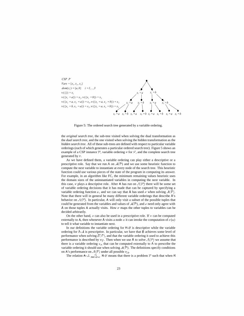
In fact we can go even further, and assume that FC-hidden explores a search treecontaining the ordinary variables only. Using one of the above restricted variable or-derings, FC-hidden will have instantiated all ordinary variables prior to instantiatingany dual variable. Due to the nature of the constraints in the hidden, once all of theordinary variables have been consistently instantiated, there will be only one consis-tent tuple in the domain of each dual variable; FC will prune away all of the other,inconsistent, tuples. FC will then proceed to descend in a backtrack free manner downthe single remaining branch to instantiate all of the dual variables. Thus we can stopthe search once all of the ordinary variables have been assigned—we already have asolution. That is, we need only consider the top part of the search tree where the or-dinary variables are being instantiated, and we can consider FC-hidden and FC-orig tobe exploring the same search tree consisting of all of the ordinary variables.

We now present examples that allow us to prove some relationships between thethree problem formulations.

Example 8 Consider a non-binary CSP with only one constraint over � Boolean vari-ables, ,N�"�#�&��'�/@ �� @3��:@��'@3�� . FC applied to this formulation visits�N� � � � nodes and performs �N� � � � consistency checks to find all solutions irrespectiveof the variable ordering used. There are only two nodes in the search tree for FC-dual,representing the two possible solutions. FC-hidden visits �N�"�� nodes and performs�N�"� � consistency checks.

25

Theorem 7 FC-orig can be super-polynomially worse than FC-dual and FC-hidden;i.e., FC-orig �� FC-dual and FC-orig �� FC-hidden.

Proof: See Example 8.

Example 9 Consider the non-binary CSP with � Boolean variables � �� and �constraints given by �� , � �#�� &� , � �#�� ,�N��>�� , � �#�� )�� . FC applied to this formulation visits � nodes and performs

� � consistency checkswhen using the static variable ordering �C�� . FC-hidden performs at least

� � � Jconsistency checks irrespective of the variable ordering used, as the domain of the dualvariable associated with the constraint � � � � �� 5� �� costs that much tofilter once any one of the ordinary variables is instantiated.

Theorem 8 FC-hidden can be super-polynomially worse than FC-orig; i.e., FC-hidden�� FC-orig.


Example 10 Consider a CSP with� � variables, � ��<� , each with domain �>J�� ,

and � constraints,

,-��"�� @ ��#�I@ ��&�>�,�8�"�� @ �� @ ��&�>�

��

,/� � ��"�� <� � �� @ �� I@ ��>�, �#�"��(�'� @ ��#� �@ ��>�

The problem is insoluble because the first � � J constraints force � � @B�� and thelast constraint forces � � �@3�� . Note that in each of the above constraints, the variable�� F merely increases the arity and the number of tuples of the constraint. Given thelexicographic static variable ordering �C�%��<� , FC-orig and FC-hidden will search� paths, ��#�0M J�� M J&� , ��0M � �� M � � , �� , ��#�0M � ��<�� M� � : at each node, there is only one value in the domain of the current variable that isconsistent with every uninstantiated variable. Thus FC-orig and FC-hidden visit �N�"� � �nodes to conclude that the problem is insoluble. However, irrespective of the variableordering used, along those paths where all of the �CF are set to the same value, FC-dualhas to instantiate at least

� ��"�� J dual variables to reach a dead-end. In particular, itmust instantiate enough of the dual variables � �%�� to allow it to conclude that��-@ �� , which will then yield a contradiction with the last dual variable � � . However,even under the restriction that each of the variables � F get the same value, FC-dualmust additionally “instantiate” a variable from � � � ��<� at each stage that has noinfluence on the failure. This will cause it to backtrack uselessly to try � different waysof setting each dual variable using different values for these variables

The best variable ordering strategy for FC-dual along these paths is to repeatedlysplit the set of ordinary variables � �� by instantiating the dual variable overthe mid-point variables, so as to most quickly derive a relation between �� and �� .

26

For example, FC-dual would first branch on the dual variable corresponding to theconstraint ,N�"�� , thus instantiating the two mid-point variables in thesequence �� . In the next two branches it would split the subproblems involv-ing �#�� and �� %�� . Continuing this way it can instantiate all of thevariables �#�� by instantiating �N� � ��"��<� dual variables and thus conclude that��I@3�� to obtain a contradiction. Once failure has been detected FC must then back-track and try the other �N�"� � consistent values of each dual variable. Hence, FC-dualhas to explore at least �N�� nodes.

Theorem 9 FC-dual can be super-polynomially worse than FC-orig and FC-hidden;i.e., FC-dual �� FC-orig and FC-dual �� FC-hidden.


Now we turn to the relation between FC-dual and FC-hidden. In Example 8, weobserve that FC-hidden visits �N�"�� times as many nodes as FC-dual does. As we nowshow, this bound is true in general. We then show that FC-hidden � �� FC-dual.

Let�

be any CSP instance, and let � �� be any variable ordering for � �'5�=�� . Wemust show that there exists a variable ordering �

�� such that the performance of

FC on� � �>��;�� using �

�� is within a polynomial of its performance on � �'5�=� � �

using � �� . First, we show how to construct � �� using � �� , then we show that

under this variable ordering a polynomial bound is achieved.Let � @ �� M EO�%��D M E�D>� be a sequence of assignments to ordinary

variables; i.e., a possible node in the search tree explored by FC-hidden. We need tocompute �

�� "�� ; i.e., the next variable to be assigned by FC-hidden when and if

it visits � . This will be the variable instantiated by the children of � . Once we cancompute � ��

� �� "�� for any node � , we will have determined the function �� , and

hence the ordered search tree generated by �� and searched by FC-hidden. To

do this we establish a correspondence between the nodes in the ordered search treegenerated by � �� , �� , and nodes that would be in the ordered search tree generatedby �

�� ,

�� . Using Theorem 6 we can consider

�� to be an ordered search

tree over only the ordinary variables (i.e., the original variables of�

).The correspondence is based on the simple observation that every assignment to a

dual variable � by FC-dual corresponds to a sequence of assignments to the ordinaryvariables in 4�5�6(7>� � � . Each node � � in

�� is a sequence of assignments to dualvariables. Let this sequence of assignments be � � �NM �<�%�� D M �D>� , where �<F isa tuple of values in the domain of the dual variable � F . Each dual variable representsa constraint (from the original formulation

�) over some set of ordinary variables.

Let 4�5�6$78� � FG� @ �� be the set of ordinary variables associated with thedual variable � F with ��F being the arity of � F . Assigning � F a value assigns a value toevery variable in 4�5�6(7>� � FG� . Given a lexicographic ordering of the ordinary variables,� F M ��F thus corresponds to a sequence of assignments to the ordinary variables in4�5�6(78� � FG� : ��&�IM ��F �&��"G�� CM ��F� � � "G� , where �! � " is the value that tuple � assignsto variable � . Thus we can convert each node � � in

� � �� , � � @ � � � M �<�%�� D M�D>� into a sequence of assignments to ordinary variables �� M �<� � � �� "G�� M�<� � � �� "G��

�� M �D� � �� "G�� M �D3 � �� "9� .

27

If no ordinary variable is assigned two different values in this sequence, then foreach variable in the sequence we can delete all but its first assignment. This will yielda non-repeating sequence of assignments to ordinary variables. The fundamental prop-erty of � ��

� �� is that each such non-repeating sequence generated by the nodes of �� will be a node in the ordered search tree

�� . We define a function, ��

from nodes of �� to the nodes of

�� . Given a node � � of

�� , �� "� �� isthe non-repeating sequence of assignments to ordinary variables generated as just de-scribed. If �� contains two different assignments to an ordinary variable, then we leave�� "� �%� undefined (in this case there is no corresponding node in

�� ).

One thing to note about the function �� is that if �� and �)� are nodes of ��

such that �� is defined on both nodes and �I� is an ancestor of �� then �� "� �� willbe a sub-sequence of or will be equal to �� "��%� . This means that either �� "� �� isthe same node as �� "�� or that �� "� �� is an ancestor of �� "�,�%� in

�� .

Example 11 For example, the sequence of assignments � � @ � � �%�"��%� M��O��J>��>� , � ��"��<��%�:M ��J>��O��>� , � ��"��>��:M ��O� �>�(� , yields the sequence of as-signments to ordinary variables �� -M � , �� M J , �� M � , �� M J , �� M � , �� M � ,�� M � , ��M �� . No variable is assigned two different values in this sequence, so�� "� �%� @ ��NM � , �� M J , �� M � , �� M J , ��M �� is the non-repeating se-quence, and this sequence of assignments will be a node in

�� . On the other hand,

the sequence � � � @ � � ��"��%�:M ��O��J%�� "��%� M ��J��>�(� has two different as-signments to �#� so �� "� � � � remains undefined, and � � � does not have a correspondingnode in

�� .

To compute �� "�� for some node � (which could be the empty set of assign-

ments) we start by setting � � @ � ; i.e. the root of �� . At each iteration �� "� �%� will

be a prefix of (or sometimes equal to) � and we will extend � � so that it covers moreof � until �� "��%� is a super-sequence of � . To extend � � we examine � �� "� �%� .Let � �� "� �%��@ � . � is the next dual variable assigned by the children of � � . Let��N@ ��&�%��D8� be the lexicographically ordered sequence of ordinary variables thatwill be newly assigned by � (these are the variables in 4�5�6$7>� � � that have not alreadybeen assigned in � � ), and let

� @ � O�%�� F � be the sequence of variables assignedby � that come after �� "� �� . (Note that either of, or both of, these sequences couldbe empty.) There are three possibilities.

1. These two sequences do not match (i.e., neither is a prefix of the other). In thiscase � does not have a matching node in

�� , and we can terminate the processand choose �

�� "�� arbitrarily.

2.�� is a sub-sequence of or is equal to

� . In this case � assigns a value to each ofthe variables � F . In addition, all of the other variables in 4�5�6(78� � � (the ones thatare not newly assigned by � ) will have been assigned by previous assignments in� . Thus there is only one tuple of values that can be assigned to � that will becompatible with � . Let this tuple be � . We check that � is in �� !� � � . If it is, then� � will have a child that makes the new assignment � M � , and we extend � � byincluding that new assignment (i.e., we move � � to this single matching child).�� "� �%� will still be a prefix of � and we can continue to the next iteration.

28

Otherwise, if � �) �� !� � � , then � has no matching node in �� and we can

terminate the process and choose �� "�� arbitrarily.

3.�� is a strict super-sequence of

� . In this case we set � �� "�� to be the first

ordinary variable �>F in�� that is unassigned by � .

The time complexity of the above process for computing �� is at most a poly-

nomial factor worse than the time complexity of � �� , as it only requires polynomialtime access to � � � �� . (In particular, we do not need to do any search in

�� to compute�� , rather we only need to follow one path of

�� .)6

Given a problem�� ;�� , the variable ordering �

�� generates an ordered

search tree�� . Using �� , we can define an “inverse” function

�� that maps

nodes of�� to nodes of

�� . The function is used in the proofs of Lemma 4 andTheorem 11. If � is a node in

�� (i.e., a non-repeating sequence of assignments

to ordinary variables that occurs in�� ) then

�� "�� is the first node of

�� in abreadth-first ordering of

�� that makes all of the same assignments as � . Formally,�� #�"�� is defined to be the shallowest (closest to the root) and leftmost node � � ) �� such that �� "� �%� is a super-sequence of � (not necessarily proper). If there isno such node in

�� then�� "�� is undefined.

Example 12 Consider the ordered search tree �� shown in Figure 6 and the corre-

sponding ordered search tree�� generated by � ��

� �� shown in Figure 7.�� IM

E�� M E�� M�� @ �)� (nodes in the diagram include all assignments madealong the arcs from the node to the root of the tree). Similarly,

�� "�� M E��<��M

E�� M��%��NM��@ �� . So additional assignments in�� do not move to new

nodes in �� if the dual node contains extra ordinary variables. On the other hand,�

� �#�"��0M E�� MAE�� M E��NMAE�� @ �� , while�� "�#� M E�� MAE��<�� M

E�� M2E�� M��C@ �� . So an additional assignment can move down through manynodes in

�� , as many as is needed to find the first descendant that assigns the newvariable. In this case we had to move down two levels to find a node assigning � � .

Lemma 4 The number of nodes in�� that are mapped to the same node in

��

by the function�� is at most � , the maximum arity of a constraint in the original

formulation.

Proof: Say that the nodes � � �� D in�� are all different and yet

�� "� � �I@

��@ �� "��D&� @ � � . By the definition of

�� , �� "� �%� must be a super-sequence

of all of these nodes. Hence, they must in fact all be of different lengths, and we canconsider them to be arranged in increasing length. We also see that ��F must be a sub-sequence of � � if �� H . �� "� �%� might be equal to � D , but it must be a proper super-sequence of all of the other nodes. Furthermore, if -� is � � ’s parent (in

�� ) then6This is an important, albeit technical point. The number of tuples in the domain of a dual variable can be

exponential in � . So a node � � might have an exponential number of child nodes. However, in this procedurewe need never search the child nodes to find the correct extension of � � . In case (2) we always know thetuple of assignments that must be the extension and we can test whether or not this extension exists with asingle constraint check. In case (3) we can compute the next variable to assign directly from the constraint’sscheme without looking at the possible assignments to the constraint.

29

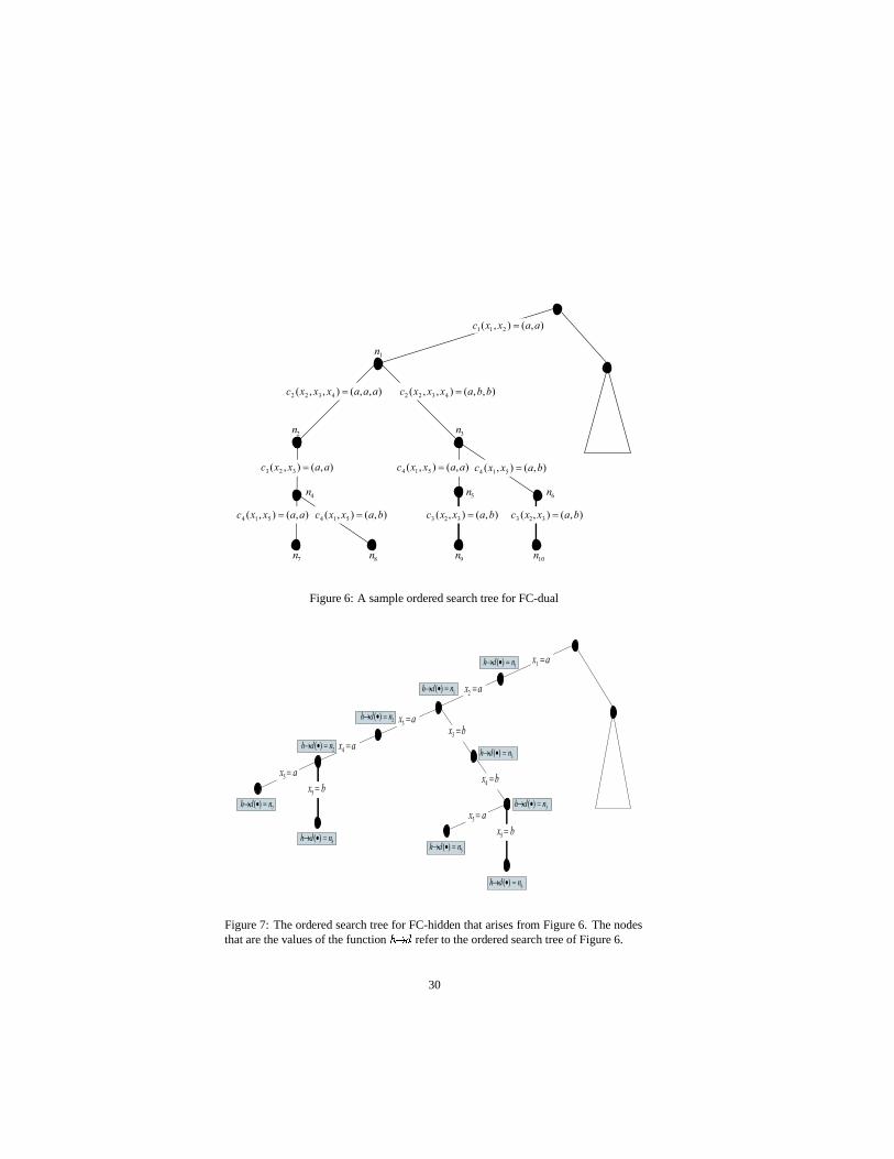
),(),( 211 aaxxc =

),,(),,( 4322 aaaxxxc =

),(),( 323 aaxxc =

),(),( 514 aaxxc =

),,(),,( 4322 bbaxxxc =

),(),( 514 baxxc =

),(),( 514 aaxxc =

),(),( 323 baxxc = ),(),( 323 baxxc =

),(),( 514 baxxc =

1n

n3

n6n5

n8n7

n4

n2

n9 n10

Figure 6: A sample ordered search tree for FC-dual

1 ax =

2 ax =

3 ax =

3 bx =

4 ax =

5 ax =

5 bx =4 bx =

5 ax =

5 bx =

1)( ndh =•→

1)( ndh =•→

2)( ndh =•→

2)( ndh =•→

8)( ndh =•→

7)( ndh =•→

3)( ndh =•→

5)( ndh =•→

6)( ndh =•→

3)( ndh =•→

Figure 7: The ordered search tree for FC-hidden that arises from Figure 6. The nodesthat are the values of the function

�� refer to the ordered search tree of Figure 6.

30

�� O� must be a proper sub-sequence of all of these nodes. (Otherwise,�� "�:��

would not be � � as � would have been a shallower node satisfying�� ’s definition.)

Since � � instantiates only one more dual variable than � , �� "� �%� can be at most� assignments (to ordinary variables) longer than �� %� . Putting these constraintstogether we see that the sequence of nodes �-�%��D can only be at most � long.

The final component we need to prove that FC-hidden � �� FC-dual is to recall acharacterization of the nodes visited by FC that is due to Kondrak and van Beek [12].Given a CSP

�and a tuple of assignments � , we say that � is consistent with a variable

if � can be extended to a consistent assignment including that variable. It is easy to seethat if an assignment � is consistent with every variable, any subtuple � � % � is alsoconsistent with every variable.

Theorem 10 (Kondrak and van Beek [12]) FC visits a node � (in the ordered searchtree it is exploring) if and only if � is consistent and its parent is consistent with everyvariable.

From this result it follows that if a node � is visited by FC and then FC subsequentlyvisits a child of � then � must be consistent with every variable. That is, all parentnodes in the search tree explored by FC must be consistent with every variable.

Theorem 11 FC-hidden can be only polynomially worse than FC-dual; i.e., FC-hidden� �� FC-dual.

Proof: Using the formalism just developed we must first show that the number ofnodes visited by FC-hidden (FC solving

�� ;�� ) using �� is within a polyno-

mial of the number of nodes visited by FC-dual (FC solving � �'5�=�� ) using � �� .That FC-hidden uses �

�� means that it searches in the tree

�� , and simi-

larly FC-dual searches in the tree �� . If � is a parent node in the sub-tree of

��

that is visited by FC, then by Theorem 10 � must be consistent with every variable.We claim that for every such parent node

�� is defined, and that FC-dual visits�

� �#�"�� in �� . We prove this claim by induction.

The base of the induction is when � is the root of�� . In this case

�� "� � is

the root of �� , and FC-dual visits it. Let � be a node that is consistent with every

variable, and let be � ’s parent. is also consistent with every variable, as we observedabove. Thus by induction

�� #� @ � is defined, and FC-dual visits it. Note that all

of � ’s ancestors must map to proper sub-sequences of (and � ) under �� , since �is the shallowest node to map to a super-sequence of . We have two cases.

1. �� %� is a proper super-sequence of . � must next assign the ordinary vari-able �

�� , which by construction must be the first ordinary variable not

assigned by in the sequence �� . Furthermore, all of � ’s siblings assignvalues to the same dual variable. Thus they all assign the same sequence of newordinary variables as �� , and in particular �� and all of its siblings must assignall of the ordinary variables assigned by � .

Let the last dual variable assigned by � be � . Since � is consistent with everyvariable, there must be at least one tuple � in �� !� � � that is consistent with � .

31

Furthermore, since � ’s parent makes fewer assignments to ordinary variablesthan does � , � ’s parent must also be consistent with � M � . (Remember thatthe dual constraints only require agreement on the shared ordinary variables).Hence, � ’s parent must have a child node making the assignment � M � , thischild node is itself consistent, and FC-dual must visit this child node. All suchchild nodes (siblings of �� ) yield super-sequences of � under the mapping �� and they are the shallowest nodes to do so: their parent maps to a proper sub-sequence of � . We may take the leftmost such child to be

�� "�� , and we have

also shown that FC-dual visits�� "�� .

2. �� %�0@ . In this case and thus � assigns every ordinary variable in thedual variables of � . Starting at � we can descend in the tree

�� . At eachstage we examine the dual variable � assigned by the children of � . If � assignsall of the variables of � , then there can be at most one tuple � in �� !� � � that isconsistent with � . Furthermore, since � is consistent with every variable, includ-ing � , such a tuple must exist. Since � makes fewer assignments to ordinaryvariables than � it too must be consistent with every variable, with � M � , and noother value in �� !� � � . Thus since FC-dual visits � it will visit the child �� of � making the assignment � M � and no other children. Now we set � to be � �and repeat the argument until we set � to be a node that makes a super-set (orthe same set) of the assignments made by � . At this point, we are back to caseone above.

So we have that for each parent node � in the sub-tree visited by FC-hidden, there isa corresponding node

�� #�"�� in the sub-tree visited by FC-dual. Furthermore, at most

� nodes can be mapped to the same node by�� (by Lemma 4), so there are at most

� times as many parent nodes visited by FC-hidden as nodes visited by FC-dual. Now,since each parent node in

�� can have at most � children (only ordinary variables

are instantiated by FC-hidden and � is the maximum number of values these variablespossess) the total number of nodes visited by FC-hidden is at most � times the numberof parent nodes visited, and at most � � times the number of nodes FC-dual visits. Tocomplete the proof, we note that both FC-dual and FC-hidden filter only dual variablesand at most 1 of them when forward checking at a node and that therefore the numberof consistency checks performed at each node are polynomially related.

We summarize the relations between FC on the different formulations in Figure 8.

4.3 Maintaining (generalized) arc consistency algorithm (MAC)

In this section, we compare the performance of an algorithm that maintains (general-ized) arc consistency or really-full lookahead [8, 16, 20] on the three models. We referto the algorithm as MAC; namely, maintaining generalized arc consistency algorithm.

We begin by characterizing the nodes visited by MAC. The algorithm enforces arcconsistency on the CSP induced by the current assignment (see Definition 5). Givena CSP and an assignment � , we say � is arc consistent if the CSP induced by � is notempty after enforcing arc consistency. It is easy to see that if an assignment � is arcconsistent, any subtuple � � % � is also arc consistent.

32

Theorem 12 MAC will visit a node � (in the ordered search tree it is exploring) if andonly if � ’s parent is arc consistent and the value assigned to the current variable by �has not been removed from its domain when enforcing arc consistency on � ’s parent.

Proof: We prove this by induction on the length of � . The claim is vacuously truewhen � is the empty sequence of assignments. Say that � is of length L , and let be� ’s parent. If � is visited then it is clear that must have yielded a non-empty CSPafter MAC enforced arc consistency on it; i.e., must have been arc consistent, and thenew assignment made at � must have survived arc consistency. Conversely, suppose was arc consistent and that � survives enforcing arc consistency at . Since is itselfarc consistent, it must have had an arc consistent parent, and it must have survivedthe enforcement of arc consistency at its parent. Hence, by induction MAC will havevisited . But then once MAC visits and enforces arc consistency there, it will havea non-empty CSP in which � survived. Thus it must continue on to visit � .

Note this also means that MAC will visit a node � (in the ordered search tree it isexploring) if � is arc consistent (as then its parent would be arc consistent, and it wouldhave survived the enforcement of arc consistency at its parent).

Just as in the case of FC-hidden, MAC-hidden does not need to instantiate all thevariables in order to find a solution. A variable ordering for MAC-hidden that instanti-ates all the ordinary variables first is at worst polynomially bounded compared to anyother variable ordering strategy.


and a variable ordering � for the hidden transformation� � ��>;�� , we can construct (in polynomial time given polynomial time access to � )a new variable ordering � � that instantiates all of the ordinary variables of

� � ��; � � � �prior to instantiating any dual variable such that MAC-hidden using � � visits at most�N�� times as many nodes as it visits when using � , where � is the arity of the largestconstraint scheme in

�.

Proof: See [4].

Given the above, we can again assume that MAC-hidden only instantiates the ordi-nary variables during its search.

We know from Theorem 1 that arc consistency on the hidden transformation isequivalent to arc consistency on the original formulation. Because MAC-orig andMAC-hidden explore the same search tree, we expect they should visit the same nodes.

Lemma 5 Given an assignment � of a CSP�

, 5�� + �� is empty iff 5��8� � � ��;�� *+ �� isempty. Furthermore, for each ordinary variable � , � has the same domain in 5��>� � + ��and 5�� ;��C� � � + �� .Proof: Since 5�� + �� is arc consistent, 5�� + �� is empty iff

� � �>��;�� <5�� + �� is empty(by Lemma 2) iff 5 �� ;�� + �� is empty (by Theorem 1). Furthermore, for each or-dinary variable � we have that �� "�� @ ��

� �� (by Corollary 1).

Now consider the two problems�� ;�� + �� and

� � ��>;�� + � . In� + � (Definition 5)

33

the domain of each ordinary variable � ) 4�5�6(78��<� is reduced to the singleton value as-signed to that variable by � , �*�! � "9� . The domains of the other variables are unaffected.However, all of the constraints of

� + � have also been reduced so that they contain onlytuples over the reduced variable domains. Thus the hidden transformation

� � ��;��C� � + ��will contain dual variables in which any tuple incompatible with � has been removed.In

� � ��;�� *+ � on the other hand, the dual variables will not be reduced, they willcontain the same set of tuples as the original constraints of

�. However, every tu-

ple in the domain of a dual variable � in� � ��; � � � � + � that is not in the domain of �

in� � ��;��C� � + �� must be arc inconsistent. It assigns an ordinary variable a value that

no longer exists in the domain of that variable. So enforcing arc consistency will re-move all of these tuples. Clearly if we sequence arc consistency so that we removethese values first, we will first transform

� � ��; � � � � + � to� � ��;�� + �� after which the

continuation of arc consistency enforcement must yield the same final CSP. That is,5�� ;�� + ��<�C@ 5�� ; � � � � + �� , and thus 5��>� � + �� is empty iff 5�� >��;�� + ��is empty. Furthermore, for every variable ��

� �� @ �>��

,and thus for every ordinary variable �� "��C@ ��

� � � �� .

Theorem 14 MAC-orig can be only polynomially worse than MAC-hidden, and viceversa; i.e., MAC-orig � �� MAC-hidden and MAC-hidden � �� MAC-orig.

Proof: Since MAC-orig and MAC-hidden search over the same variables, the samevariable ordering can be used by both formulations. Let � be the variable orderingused and let

� be the ordered search tree induced by � for a CSP

�. Both MAC-

orig and MAC-hidden will search in� . We show that they both visit the same nodes

in� . The parent of node � is arc consistent in

�iff 5�� + �8� is not empty (by

definition) iff 5�� ;��C� � � + �>� is not empty (by Lemma 5) iff is arc consistent in� � ��>;�� . Furthermore, once we enforce arc consistency at in�

the domains of allof the uninstantiated (ordinary) variables will be the same as their domains in 5�� +��>�which will be the same as their domains in 5��>� � � ��;�� + �� (by Lemma 5). Thus� will survive arc consistency enforcement at in

�iff it survives arc consistency

enforcement at in� � ��;�� . Hence, by Theorem 12, MAC will visit � in

�iff

MAC visits � in� � ��;�� .

To complete the proof, we note that arc consistency on a CSP�

takes �N�"1 � �� timein the worst case and arc consistency on

�� ;�� takes � �"1 � � � � � � time [2], where� , 1 , and � denote the size of the largest domain, the number of constraints, and thearity of the largest constraint scheme in

�, respectively.

The following example shows that MAC-orig and MAC-hidden can be exponen-tially better than MAC-dual.

Example 13 Consider a CSP with � �*� �"� � J%� � � variables � �� , and O� , �� , � � � � �� , each with domain �>J�� J&� , and � �� J%� � � constraints,

,N�"��&��&� �� @ ��#��@ ��&�>�,N�"��&��&� �� @ ��#��@ ��&�>�

��

,N�"�� &�<�� @ �� @ ��

34

It is a pigeon-hole problem with an extra variable #F in each constraint. The pigeon-holeproblem is insoluble but highly locally consistent. MAC-orig and MAC-hidden haveto instantiate at least � � � variables before an induced CSP is empty after enforcingarc consistency and they visit �N�� nodes to conclude the problem is insoluble. Itcan be seen that MAC-dual has the same pruning power as MAC-orig because eachpair of original constraints share at most one variable. However, at each node of thedual search tree, MAC-dual has to additionally instantiate a variable �F , which has noinfluence on the failure. As a result, MAC-dual has to explore a factor of �N�"� � � morenodes and is thus exponentially worse than MAC-orig and MAC-hidden.

The following example shows the converse: if two original constraints share morethan one variable, arc consistency on the dual is tighter than on the original formulation,and MAC-dual can be super-polynomially better than MAC-orig and MAC-hidden.

Example 14 Consider a CSP with �� variables, � �%��(� � � , each with domain�>J��$�� , and

� � � J constraints,

,N�"�#��&��&� @ �8�"�#� � �� @ �"�� (�>�,N�"��>��&�� @ �8�"�� @ �"�� (�>�

��

,N�"��(� � ��(��(� � �%��(� � �� @ �8�"��(� � � � ��(� � �� @ �"��(� � � � ��(� � � � �� (�>�,N�"��(� � ��(� � ��%�� @ �8�"��(� � � � ��(� � � � �� @ �"�� (�>�

�"�� @ � implies �"�� @ J implies �"�� @ � im-plies �� implies �"��(� � � ��$� � � � �� C@ � . But then the last constraint also implies�"�� !�� @ J . Thus the problem is insoluble. When enforcing arc consistencyat a node in the original search tree, no values will be removed from the domain of anordinary variable unless the variable is the last uninstantiated variable in a constraint.The best variable ordering strategy in the original formulation is to divide the prob-lem in half by first branching on the variables � � , �� , ��<� � � and � �<� � � . Then we canbranch on an insoluble subproblem consisting of ��<� , or � �<� � ��(� � � .By this divide-and-conquer approach, the maximum depth of the original search treeis �N� � ��"��<� and the number of nodes explored by MAC-orig and MAC-hidden is�N�"� � �� . In the dual transformation, on the other hand, the dual constraints forma cycle in the constraint graph. Once a dual variable is instantiated, the cycle is bro-ken so that the induced CSP is empty after enforcing arc consistency. Thus MAC-dualonly needs to instantiate one variable to conclude the problem is insoluble and it visits�N�"� � � nodes. MAC-dual is therefore super-polynomially better than MAC-orig andMAC-hidden.

Theorem 15 MAC-dual can be super-polynomially worse than MAC-orig and MAC-hidden; i.e., MAC-dual �� MAC-orig and MAC-dual �� MAC-hidden.


Theorem 16 MAC-orig and MAC-hidden can be super-polynomially worse than MAC-dual; i.e., MAC-orig �� MAC-dual and MAC-hidden �� MAC-dual.

35


MAC-dual can be super-polynomially better because it enforces a stronger consis-tency on the dual transformation and MAC-hidden can be super-polynomially betterbecause it makes fewer instantiations at each stage during the backtracking search.

Figure 8 summarizes our results. For completeness, we summarize in the diagramour results for the chronological backtracking algorithm (BT). However, for reasons oflength, we do not present the proofs of these results. Such proofs, using an alternativeformalization, can be found in [4]. As can be seen, BT-dual can be only polynomiallyworse than BT-hidden, and vice versa. On the other hand, BT-dual and BT-hidden canbe super-polynomially worse than BT-orig, and vice versa.

Also included in the diagram are results due to Kondrak and van Beek [12] betweendifferent algorithms applied to the same problem formulation. For example, considerthe relation FC-hidden � �� BT-hidden. Since the same problem is being solved, Kon-drak and van Beek’s result that FC always visits the same or fewer nodes than BT, canbe directly applied.7 Then, since arc consistency is � �"1 � � � and forward checking is�N�"1#�8� for binary problems with 1 constraints and domain size � , it follows that FC-hidden � �� BT-hidden. Interestingly, although it is easily shown that MAC-orig alwaysvisits the same or fewer nodes than FC-orig, we have that MAC-orig �� FC-orig,since there exist problems where MAC-orig can perform exponentially more constraintchecks than FC-orig.

Furthermore, we can use properties of � �� to draw additional conclusions from thediagram. Whenever we are comparing formulations that are all polynomially related insize the relation � �� is transitive. Thus, for example, since the hidden and dual transfor-mations (although exponentially larger than the original formulation) are polynomiallyrelated in size, from MAC-hidden � �� FC-hidden and FC-hidden � �� FC-dual, we canconclude that MAC-hidden � �� FC-dual. Similarly, from MAC-dual � �� FC-dual andFC-dual � �� BT-dual, we can conclude that MAC-dual � �� BT-dual. Note that the

�� relation is not transitive. So, for example, we cannot conclude that since FC-hidden �� FC-orig and FC-orig �� FC-dual we have that FC-hidden �� FC-dual. In fact, as shown in Theorem 11, FC-hidden � �� FC-dual.

5 Conclusion

We compared three possible models for a constraint satisfaction problem—the originalformulation, the dual transformation, and the hidden transformation—with respect tothe effectiveness of various local consistency properties and the performance of threedifferent backtracking algorithms. To our knowledge, this is the first comprehensiveattempt to evaluate constraint modeling techniques in a formal way.

We studied arc consistency on the original formulation, and its dual and hiddentransformations. We showed that arc consistency on the dual transformation is tighter

7Kondrak and van Beek prove their results for static variable orderings. However, their results also hold

when the algorithm searches a fixed ordered search tree, as is allowed by the definition of � �� .

36

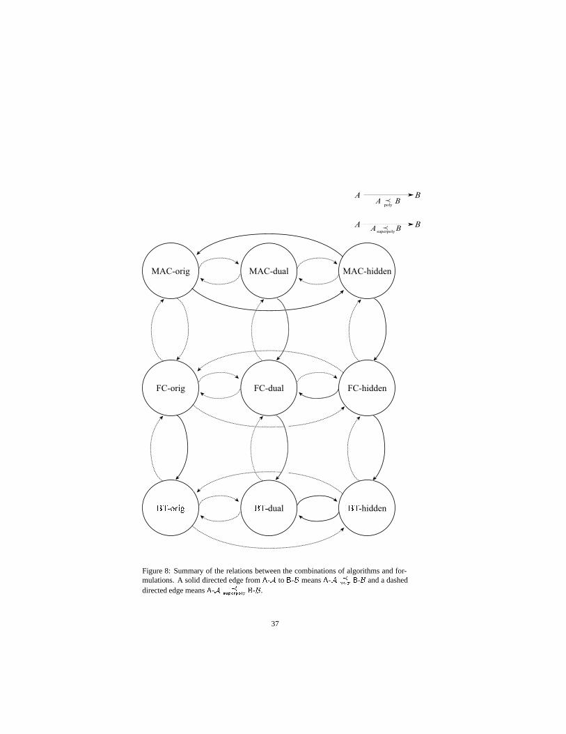
�� dual

� ��hidden

FC-orig FC-dual FC-hidden

MAC-orig MAC-dual MAC-hidden

A

A

B

B

pA B

pA B

poly

superpoly

Figure 8: Summary of the relations between the combinations of algorithms and for-mulations. A solid directed edge from

�- � to - � means

�- � � �� - � and a dashed

directed edge means�

- � �� - � .

37

than arc consistency on the original formulation, which itself is equivalent to arc con-sistency on the hidden transformation. We then considered local consistencies that aredefined over binary constraints. For example, we showed that singleton arc consistencyon the dual is tighter than singleton arc consistency on the hidden.

We then compared the performance of three different backtracking algorithms on anon-binary CSP and on its dual and hidden transformations. Considering the forwardchecking algorithm, FC-dual can be super-polynomially worse than FC-orig and FC-hidden, and FC-orig can be super-polynomially worse than FC-dual and FC-hidden.However, the cost to solve FC-hidden can be at most a polynomial factor worse thanthe cost to solve FC-dual. Turning to the algorithm that maintains arc consistency,MAC-orig and MAC-hidden visit the same nodes and have the same cost at each node,while MAC-dual can be super-polynomially worse than MAC-orig and MAC-hiddenbecause it may have to make many more instantiations at each node of the searchtree. Furthermore, MAC-orig and MAC-hidden can be super-polynomially worse thanMAC-dual because MAC-dual enforces a stronger consistency property than MAC-orig or MAC-hidden do.

Our results can be used by practitioners to help build efficient models for real-worldconstraint satisfaction problems. Our objective is to provide some general guidelines asto whether or not, or under which conditions, the dual or hidden transformation shouldbe applied to a non-binary CSP. For example, if the performance of formulation � isbounded by a polynomial from formulation � but can be super-polynomially betterthan � , then we are assured that the performance of � cannot be much worse than thatof � , and that furthermore � has the potential to provide a dramatic improvement over� . Thus, � may be preferred in the hope that it can provide super-polynomial savingsover � and given that in the worst case, it cannot lose too much. On the other hand, iftwo formulations are equivalent for a certain backtracking algorithm, there is little tobe gained from developing both models.

References

[1] F. Bacchus and P. van Beek. On the conversion between non-binary and binaryconstraint satisfaction problems. In Proceedings of the Fifteenth National Con-ference on Artificial Intelligence, pages 311–318, Madison, Wisconsin, 1998.

[2] C. Bessiere and J.-C. Regin. Arc consistency for general constraint networks:Preliminary results. In Proceedings of the Sixteenth International Joint Confer-ence on Artificial Intelligence, pages 398–404, Nagoya, Japan, 1997.

[3] J. E. Borrett. Formulation Selection for Constraint Satisfaction Problems: AHeuristic Approach. PhD thesis, University of Essex, United Kingdom, 1998.

[4] X. Chen. A Theoretical Comparison of Selected CSP Solving and Modeling Tech-niques. PhD thesis, University of Alberta, Canada, 2000.

[5] R. Debruyne and C. Bessiere. Domain filtering consistencies. J. Artificial Intelli-gence Research, 14:205–230, 2001.

38

[6] R. Dechter. On the expressiveness of networks with hidden variables. In Proceed-ings of the Eighth National Conference on Artificial Intelligence, pages 556–562,Boston, Mass., 1990.

[7] R. Dechter and J. Pearl. Tree clustering for constraint networks. Artificial Intelli-gence, 38:353–366, 1989.

[8] J. Gaschnig. Experimental case studies of backtrack vs. Waltz-type vs. new algo-rithms for satisficing assignment problems. In Proceedings of the Second Cana-dian Conference on Artificial Intelligence, pages 268–277, Toronto, Ont., 1978.

[9] L. Getoor, G. Ottosson, M. Fromherz, and B. Carlson. Effective redundant con-straints for online scheduling. In Proceedings of the Fourteenth National Confer-ence on Artificial Intelligence, pages 302–307, Providence, Rhode Island, 1997.

[10] R. M. Haralick and G. L. Elliott. Increasing tree search efficiency for constraintsatisfaction problems. Artificial Intelligence, 14:263–313, 1980.

[11] P. Jegou. Decomposition of domains based on the micro-structure of finite con-straint satisfaction problems. In Proceedings of the Eleventh National Conferenceon Artificial Intelligence, pages 731–736, Washington, DC, 1993.

[12] G. Kondrak and P. van Beek. A theoretical evaluation of selected backtrackingalgorithms. Artificial Intelligence, 89:365–387, 1997.

[13] A. K. Mackworth. Consistency in networks of relations. Artificial Intelligence,8:99–118, 1977.

[14] A. K. Mackworth. On reading sketch maps. In Proceedings of the Fifth Inter-national Joint Conference on Artificial Intelligence, pages 598–606, Cambridge,Mass., 1977.

[15] J. J. McGregor. Relational consistency algorithms and their application in findingsubgraph and graph isomorphisms. Inform. Sci., 19:229–250, 1979.

[16] B. A. Nadel. Constraint satisfaction algorithms. Computational Intelligence,5:188–224, 1989.

[17] B. A. Nadel. Representation selection for constraint satisfaction: A case studyusing � -queens. IEEE Expert, 5:16–23, 1990.

[18] C. S. Peirce. In C. Hartshorne and P. Weiss, editors, Collected Papers, Vol. III.Harvard University Press, 1933. Cited in: F. Rossi, C. Petrie, and V. Dhar, 1989.

[19] F. Rossi, C. Petrie, and V. Dhar. On the equivalence of constraint satisfactionproblems. Technical Report ACT-AI-222-89, MCC, Austin, Texas, 1989. Ashorter version appears in ECAI-90, pages 550-556.

[20] D. Sabin and E. C. Freuder. Contradicting conventional wisdom in constraintsatisfaction. In Proceedings of the 11th European Conference on Artificial Intel-ligence, pages 125–129, Amsterdam, 1994.

39

[21] H. Simonis. Standard models for finite domain constraint solving. Tutorial pre-sented at PACT’97 Conference, London, UK, 1997.

[22] B. Smith, S. C Brailsford, P. M. Hubbard, and H. P. Williams. The progressiveparty problem: Integer linear programming and constraint programming com-pared. Constraints, 1:119–138, 1996.

[23] K. Stergiou and T. Walsh. Encodings of non-binary constraint satisfaction prob-lems. In Proceedings of the Sixteenth National Conference on Artificial Intelli-gence, pages 163–168, Orlando, Florida, 1999.

[24] P. van Beek and X. Chen. CPlan: A constraint programming approach to plan-ning. In Proceedings of the Sixteenth National Conference on Artificial Intelli-gence, pages 585–590, Orlando, Florida, 1999.

[25] P. Van Hentenryck. Constraint Satisfaction in Logic Programming. MIT Press,1989.

[26] R. Weigel, C. Bliek, and B. Faltings. On reformulation of constraint satisfactionproblems. In Proceedings of the 13th European Conference on Artificial Intelli-gence, pages 254–258, Brighton, United Kingdom, 1998.

40

binary vs. non-binary constraints - department of computer ...fbacchus/papers/bcvwaij02.pdf ·...

Documents