binary solid mixtures - uni-greifswald
TRANSCRIPT

©Matthias Eschrig
Binary solid mixtures

©Matthias Eschrig
What happens when we cool down a mixture of chemical elements?
• At high temperatures, in the gaseous phase, all atoms mix, resulting in a single phase.
• In liquid phase they often mix perfectly, but can occasionally also show partial
immiscibility (like for example “emulsions” like milk-oil mixtures).
• In solid phase often phase separation between solution of element B in element A (α-
phase) and solution of element A in element B (β-phase) exists – a binary alloy.
• The phase transition from liquid to solid phase in such mixtures shows a characteristic
phase diagram, in which three components react with each other (e.g. liquid, α-phase,
β-phase).
• These reactions are classified into eutectic, peritectic and monotectic.
©Matthias Eschrighttp://resource.npl.co.uk/mtdata/phdiagrams/png/cuni.png
http://resource.npl.co.uk/mtdata/phdiagrams/png/nipd.png
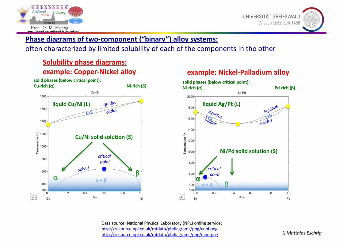
Phase diagrams of two-component (“binary”) alloy systems:
often characterized by limited solubility of each of the components in the other
Solubility phase diagrams:
example: Copper-Nickel alloy example: Nickel-Palladium alloy
Data source: National Physical Laboratory (NPL) online service:
liquid Ag/Pt (L)liquid Cu/Ni (L)
Cu/Ni solid solution (S)
solid phases (below critical point):
Cu-rich (α) Ni-rich (β)
L+S
α + β
solid phases (below critical point):
Ni-rich (α) Pd-rich (β)
αβ
βα
α + β
Ni/Pd solid solution (S) critical
point
critical
point
L+SL+S
liquidus
solidus
solvus
solidus
liquidus
solidus
liquidus

liquid Cu/Ni (L)
Cu/Ni solid solution (S)
solid phases (below critical point):
Cu-rich (α) Ni-rich (β)
L+S
α + β
l
αβ
critical
point
liquidus
solidus
solvus
©Matthias Eschrighttp://resource.npl.co.uk/mtdata/phdiagrams/png/cuni.pngData source: National Physical Laboratory (NPL) online service:
lever rule for relative
fraction of phases
wS wL
L
S
wL+wS=1
L
L
S
S
α
β

©Matthias Eschrighttp://resource.npl.co.uk/mtdata/phdiagrams/png/agpt.png
http://resource.npl.co.uk/mtdata/phdiagrams/png/agcu.png
Phase diagrams of two-component (“binary”) alloy systems:
often characterized by limited solubility of each of the components in the other
Eutectic phase diagram
example: Silver-Copper alloy
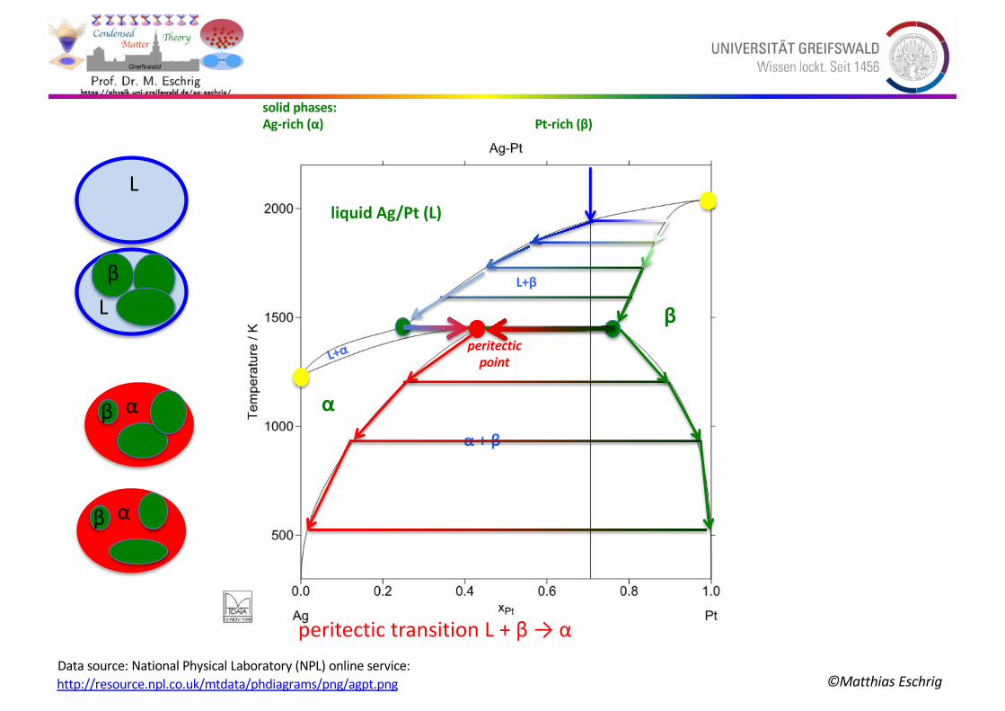
Peritectic phase diagram
example: Silver-Platinum alloy
Data source: National Physical Laboratory (NPL) online service:
liquid Ag/Pt (L)
α + β
L+β
L+α peritectic
point
peritectic transition L + β → α
liquid Ag/Cu (L)
α + β
solid phases:
Ag-rich (α) Cu-rich (β)
L+βL+α
eutectic
point
eutectic transition: L → α + β
solid phases:
Ag-rich (α) Pt-rich (β)
αβ
β
α

liquid Ag/Cu (L)
α + β
solid phases:
Ag-rich (α) Cu-rich (β)
L+βL+α
eutectic
point
eutectic transition: L → α + β
αβ
©Matthias Eschrighttp://resource.npl.co.uk/mtdata/phdiagrams/png/agcu.png
Data source: National Physical Laboratory (NPL) online service:
L
α/β

liquid Ag/Cu (L)
α + β
solid phases:
Ag-rich (α) Cu-rich (β)
L+βL+α
eutectic
point
eutectic transition: L → α + β
αβ
©Matthias Eschrighttp://resource.npl.co.uk/mtdata/phdiagrams/png/agcu.png
Data source: National Physical Laboratory (NPL) online service:
L
α/β
β
L
β
α/β
β

©Matthias Eschrighttp://resource.npl.co.uk/mtdata/phdiagrams/png/agpt.png
Data source: National Physical Laboratory (NPL) online service:
liquid Ag/Pt (L)
α + β
L+β
L+α peritectic
point
peritectic transition L + β → α
solid phases:
Ag-rich (α) Pt-rich (β)
β
α
L
L
β
α
β
α
©Matthias Eschrighttp://resource.npl.co.uk/mtdata/phdiagrams/png/agpt.png
Data source: National Physical Laboratory (NPL) online service:
liquid Ag/Pt (L)
α + β
L+β
L+α peritectic
point
peritectic transition L + β → α
solid phases:
Ag-rich (α) Pt-rich (β)
β
α
L
L
β
β α
β α
©Matthias Eschrighttp://resource.npl.co.uk/mtdata/phdiagrams/png/agpb.png
http://resource.npl.co.uk/mtdata/phdiagrams/png/cumg.png
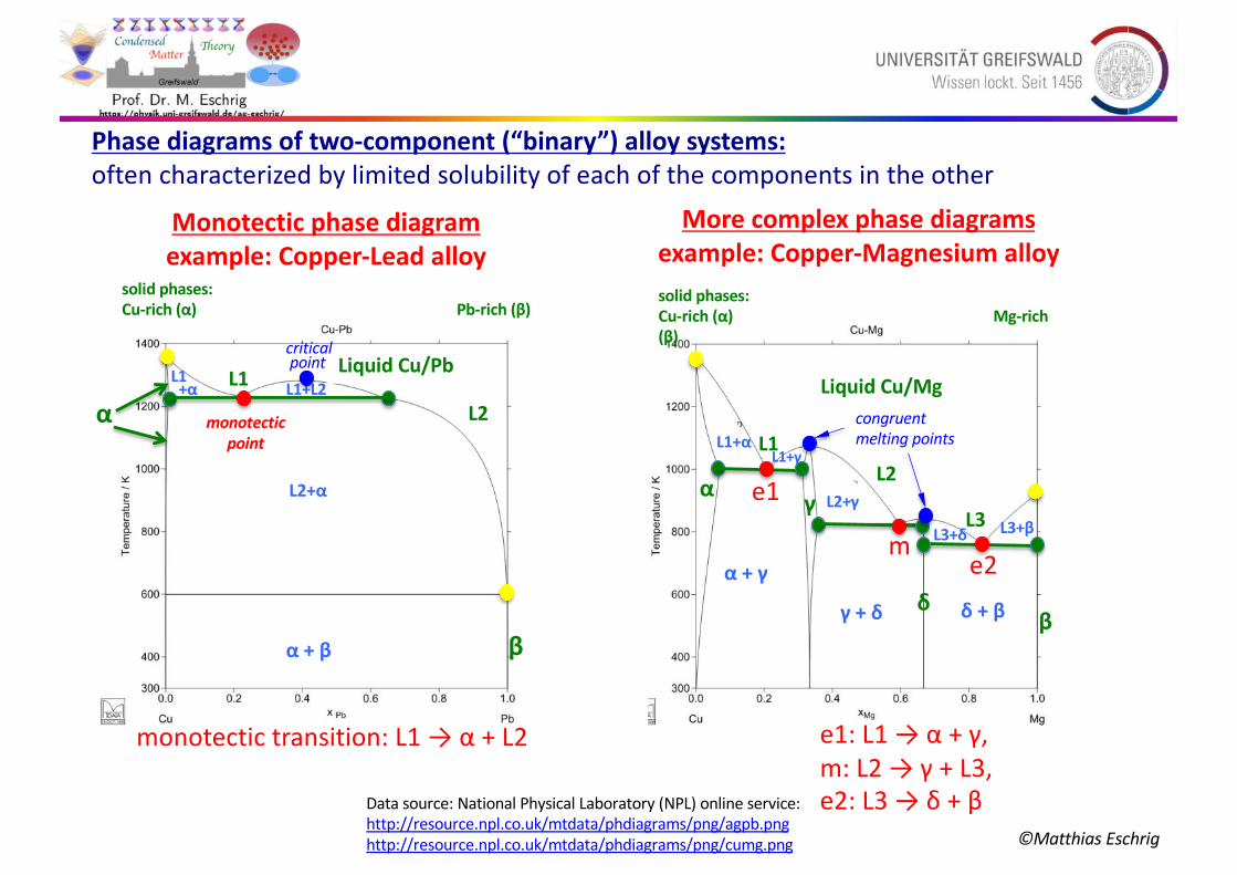
Phase diagrams of two-component (“binary”) alloy systems:
often characterized by limited solubility of each of the components in the other
Monotectic phase diagram
example: Copper-Lead alloy
More complex phase diagrams
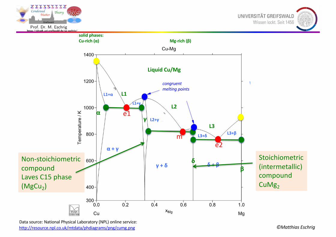
example: Copper-Magnesium alloy
Data source: National Physical Laboratory (NPL) online service:
Liquid Cu/Mg
γ + δ
α
L+sAg
peritectic
point
e1: L1 → α + γ,
m: L2 → γ + L3,
e2: L3 → δ + β
Liquid Cu/Pb
α + β
αL1+L2
L2+α
monotectic
point
monotectic transition: L1 → α + L2
L1
L2
L1+α
solid phases:
Cu-rich (α) Pb-rich (β)solid phases:
Cu-rich (α) Mg-rich
(β)
β
γ
β
L1+α L1
L2
L2+γ
L1+γ
L3 L3+β
δ
L3+δ
δ + β
α + γ
e1
me2
congruent
melting points
criticalpoint
Liquid Cu/Mg
γ + δ
α
L+sAg
peritectic
point
solid phases:
Cu-rich (α) Mg-rich (β)
γ
β
L1+α L1
L2
L2+γ
L1+γ
L3L3+β
δ
L3+δ
δ + β
α + γ
e1
me2
congruent
melting points
©Matthias Eschrighttp://resource.npl.co.uk/mtdata/phdiagrams/png/cumg.png
Data source: National Physical Laboratory (NPL) online service:
Stoichiometric
(intermetallic)
compound
CuMg2
Non-stoichiometric
compound
Laves C15 phase
(MgCu2)

©Matthias Eschrig
1.) Gibbs free enthalpy of a real binary mixture at constant pressure:
G(T,xB)/Ν = xA μA,0(T)+xB μB,0(T) + kBT (xA ln xA + xB ln xB) + xA xB [a(T)+(xA-xB) b(T)]
(Note that xA=1−xB)
Interpolates linearly
Between pure
compound Gibbs FE’s
Contribution due to
“mixing entropy”; this
term is always negative.
“Excess enthalpy”; quantifies
deviation from ideal behavior.
Can be positive or negative.
a and b are functions of T
The excess enthalpy is due to the fact that the average energy for interactions between A and B
atoms is not the same as that for A-A and B-B interactions.
In so-called ideal mixtures it is negligible (this defines ideal mixtures). This term also is zero in
the pure compounds. If the attractive interactions between A-B are on average weaker than that
for A-A and B-B, this term is positive.
The second term is due to the mixing of atoms A and B. It is zero in the pure compounds and
negative in between.
The first term is a linear function of xB that interpolates between the Gibbs free enthalpies of
the pure compounds.
Thermodynamics background: Consider two chemical components, A and B (e.g. A=Ag, B=Cu).
For each phase of a binary mixture the Gibbs free energy is given as:

©Matthias Eschrig
The construction of the lower convex hull to two curves:
Find the set of all tangents to the two curves that fulfill the condition to lie entirely below
both curves. Then find the envelope for these tangents (the “caustic”). The picture above
illustrates the procedure.
In our case it is the correct construction to find the equilibrium state between two phases from
the two Gibbs free energy curves of each phase. The red and blue curves will e.g.
correspond to the liquid and solid phases, and the green line to the coexistence region. It is
defined as a tangent to both the red and blue curves. The envelope curve (red+green+blue)
defines the thermodynamic stable state.

©Matthias Eschrig
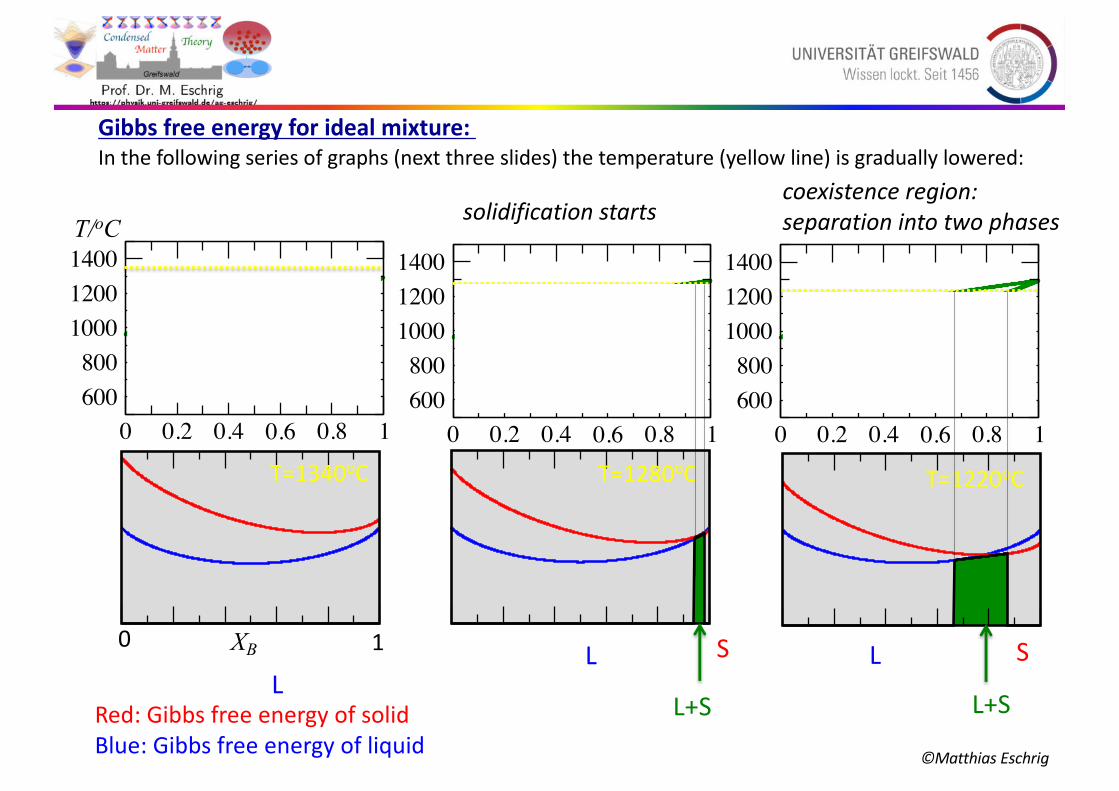
Gibbs free energy for ideal mixture:
Ideal mixtures are mixtures where the excess enthalpy term can be neglected:
G(T,xB)/N = xA μA,0(T)+xB μB,0(T) + kBT (xA ln xA + xB ln xB)
kBT (xA ln xA + xB ln xB)
xA μA,0(T)+xB μB,0(T)
G(T,xB)/N
0 1XB
A BA/B mixture
T=const.
Let us fix T and study the qualitative dependence on xB:
0

©Matthias Eschrig
Gibbs free energy for ideal mixture:
There is a version for the liquid state, GL(T,xB)/NL, and a version for the solid state, GS(T,xB)/NS .
Each of these versions of this equation has its own set of parameters.
When lowering temperature, the chemical potentials μA,0S(T) and μB,0
S(T) for the solid increase
less rapidly than μA,0L(T) and μB,0
L(T) for the liquid, as the pure solid phases must have a lower
Gibbs free energy at low temperatures than the pure liquid phases.
The mixing entropy term decreases in magnitude with decreasing temperature (it is ~T ).
NA[μA,0S(T)-μA,0
L(T)]=(-59725 + 48.35 T) J/mol
NA[μB,0S(T)-μB,0
L(T)]=(-75270 + 48.10 T) J/mol
μA,0L(T)=μB,0
L(T)
In the following pictures we take a model material with the following parameters (all
parameters are related to 1 mol, i.e. to Avogadro’s number NA=6.022x10²³ mol-1):
Ideal mixtures are mixtures where the excess enthalpy term can be neglected:
G(T,xB)/N = xA μA,0(T)+xB μB,0(T) + kBT (xA ln xA + xB ln xB)
kB=1.38x10⁻²³ J/K
NAkB=R=8.314 J/(mol K)
mixing entropylinear term
0 0.2 0.4 0.6 0.8 0
0 0.2 0.4 0.6 0.8 1
600
800
1000
1200
1400
0 0.2 0.4 0.6 0.8 1
600
800
1000
1200
1400
0 0.2 0.4 0.6 0.8 1
600
800
1000
1200
1400
©Matthias Eschrig
T=1280oC
Gibbs free energy for ideal mixture:
LL L S
L+SL+S
S
solidification starts
T=1340oC
T/oC
XB0 1
coexistence region:
separation into two phases
Red: Gibbs free energy of solid
Blue: Gibbs free energy of liquid
T=1220oC
In the following series of graphs (next three slides) the temperature (yellow line) is gradually lowered:

0 0.2 0.4 0.6 0.8 0
0 0.2 0.4 0.6 0.8 1
600
800
1000
1200
1400
0 0.2 0.4 0.6 0.8 1
600
800
1000
1200
1400
0 0.2 0.4 0.6 0.8 1
600
800
1000
1200
1400
©Matthias Eschrig
LL L S
L+S
Gibbs free energy for ideal mixture:
T/oC
XB0 1 S
SL+S L+S
Red: Gibbs free energy of solid
Blue: Gibbs free energy of liquid
T=1160oC T=1100oC T=1040oC

0 0.2 0.4 0.6 0.8 1
600
800
1000
1200
1400
0 0.2 0.4 0.6 0.8 1
600
800
1000
1200
1400
0 0.2 0.4 0.6 0.8 1
600
800
1000
1200
1400
©Matthias Eschrig
T=980oC T=920oC
L S SS
L+S
Gibbs free energy for ideal mixture:
0 0.2 0.4 0.6 0.8 1
T/oC
XB0 1
T=860oC
solidification about
to be finished
solidification is finished
no liquid left
“liquidus line”
“solidus line”
Red: Gibbs free energy of solid
Blue: Gibbs free energy of liquid

©Matthias Eschrig
2.) Composition and substance fraction of phases:
0 0.2 0.4 0.6 0.8 1
600
800
1000
1200
1400
x1x2x3x4
T1
T3
T2
A) What is the composition of the phases?
L
α
L α
T1
T2
T3
x
x x1
x3 x2
x4 x
above T1 there is only
liquid with composition x
below T3 there is only
solid with composition x
Between T1 and T3 the composition of the liquid changes from x to x4 and the composition
of the solid changes from x1 to x.

©Matthias Eschrig
0 0.2 0.4 0.6 0.8 1
600
800
1000
1200
1400
x2x3
T2
B) What is the fraction of each of the two phases?
L
α
x
sαsLwα + wL = 1
wα sα+ wL sL= sα + sL
wα= sL/(sα+sL)=(x-x3)/(x2-x3)
wL= sα/(sα+sL)=(x2-x)/(x2-x3)
“Lever rule”:
2.) Composition and substance fraction of phases:

©Matthias Eschrig
In real mixtures the excess term becomes important:
G(T,xB)/N = xA μA,0(T)+xB μB,0(T) + kBT (xA ln xA + xB ln xB) + xA xB [a(T)+(xA-xB) b(T)]
Again, there is a version pf this equation for the liquid phase, GL(T,xB)/NL, and a version for the
solid phase, GS(T,xB)/NS. Each of these versions has its own set of parameters.
NA[μA,0S(T)-μA,0
L(T)]=(-59725 + 48.35 T ) J/mol
NA[μB,0S(T)-μB,0
L(T)]=(-75270 + 48.10 T ) J/molμA,0
L(T)=μB,0L(T)
In the following pictures we take a model material with the following parameter set:
3.) Gibbs free energy leading to a miscibility gap:
aS(T)=(20719.2 – 5.5068 T ) J/mol
bS(T)=(-3597.6 + 1.035 T ) J/mol
aL(T)=(9102.6 – 1.5222 T ) J/mol
bL(T)=(-1455 + 0.5676 T ) J/molNAkB=R=8.314 J/(mol K)
mixing entropy excess enthalpylinear term

0 0.2 0.4 0.6 0.8 0
©Matthias Eschrig
1 0 0.2 0.4 0.6 0.8 1
600
800
1000
1200
12001 0 0.2 0.4 0.6 0.8 1
600
800
1000
1200
12001 0 0.2 0.4 0.6 0.8 1
600
800
1000
1200
1200T=1130.7oC
L L L S
L+S
T/oC
XB0 1
Red: Gibbs free energy of solid
Blue: Gibbs free energy of liquid
T=990.7oCT=1060.7oC
In the following series of graphs (next three slides) the temperature (yellow line) is gradually lowered:

0 0.2 0.4 0.6 0.8 0
©Matthias Eschrig
1 0 0.2 0.4 0.6 0.8 1
600
800
1000
1200
12001 0 0.2 0.4 0.6 0.8 1
600
800
1000
1200
12001 0 0.2 0.4 0.6 0.8 1
600
800
1000
1200
1200
SSSSS LL
L+S L+S
T/oC
XB0 1
Red: Gibbs free energy of solid
Blue: Gibbs free energy of liquid
T=780.7oCT=850.7oCT=920.7oC

0 0.2 0.4 0.6 0.8 1
©Matthias Eschrig
1 0 0.2 0.4 0.6 0.8 1
600
800
1000
1200
12001 0 0.2 0.4 0.6 0.8 1
600
800
1000
1200
12001 0 0.2 0.4 0.6 0.8 1
600
800
1000
1200
1200
T=710.7oC
S α β βαα+β α+β
miscibility gap miscibility gap
Mixture of two phases: α and β
T/oC
XB0 1
Red: Gibbs free energy of solid
Blue: Gibbs free energy of liquid
T=640.7oC T=570.7oC
©Matthias Eschrig
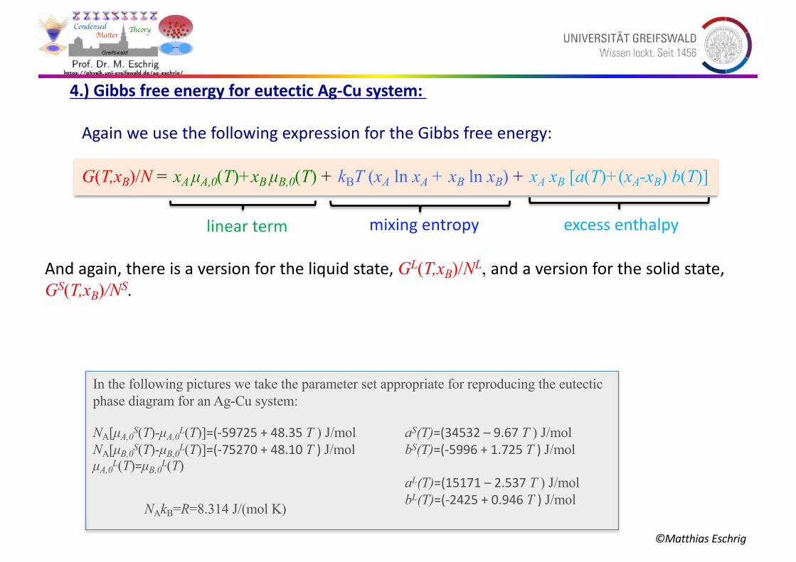
And again, there is a version for the liquid state, GL(T,xB)/NL, and a version for the solid state,
GS(T,xB)/NS.
NA[μA,0S(T)-μA,0
L(T)]=(-59725 + 48.35 T ) J/mol
NA[μB,0S(T)-μB,0
L(T)]=(-75270 + 48.10 T ) J/molμA,0
L(T)=μB,0L(T)
In the following pictures we take the parameter set appropriate for reproducing the eutectic
phase diagram for an Ag-Cu system:
aS(T)=(34532 – 9.67 T ) J/mol
bS(T)=(-5996 + 1.725 T ) J/mol
aL(T)=(15171 – 2.537 T ) J/mol
bL(T)=(-2425 + 0.946 T ) J/mol
4.) Gibbs free energy for eutectic Ag-Cu system:
Again we use the following expression for the Gibbs free energy:
G(T,xB)/N = xA μA,0(T)+xB μB,0(T) + kBT (xA ln xA + xB ln xB) + xA xB [a(T)+(xA-xB) b(T)]
NAkB=R=8.314 J/(mol K)
mixing entropy excess enthalpylinear term

©Matthias Eschrig
0 0.2 0.4 0.6 0.8 1
600
800
1000
1200
12001 0 0.2 0.4 0.6 0.8 1
600
800
1000
1200
1200
0 0.2 0.4 0.6 0.8 1
0 0.2 0.4 0.6 0.8 1
600
800
1000
1200
1
1 0 0.2 0.4 0.6 0.8 1
1 0 0.2 0.4 0.6 0.8 1
600
800
1000
1200
1
1 0 0.2 0.4 0.6 0.8 1
1 0 0.2 0.4 0.6 0.8 1
600
800
1000
1200
1
1 0 0.2 0.4 0.6 0.8 1
600
800
1000
1200
1200
Transition from ideal to eutectic phase diagram with increasing excess enthalpy(obtained by scaling the excess enthalpy part of the Gibbs free energy for both solid and
liquid by the six factors 0.4, 0.5, 0.6, 0.7, 0.8, 0.9 for the six graphs shown)
pre
ssu
re

0 0.2 0.4 0.6 0.8 0
©Matthias Eschrig
4.) Gibbs free energy for eutectic Ag-Cu system:
0 0.2 0.4 0.6 0.8 1500
600
700
800
900
1000
1100
1200
0 0.2 0.4 0.6 0.8 1500
600
700
800
900
1000
1100
1200
0 0.2 0.4 0.6 0.8 1500
600
700
800
900
1000
1100
1200
T=1130.7oC T=1060.7oC T=990.7oC
L L L ββ
L+β L+βRed: Gibbs free energy of solid
Blue: Gibbs free energy of liquid
T/oC
XB0 1
In the following series of graphs (next three slides) the temperature (yellow line) is gradually lowered:

0 0.2 0.4 0.6 0.8 0
©Matthias Eschrig
Gibbs free energy for eutectic Ag-Cu system:
0 0.2 0.4 0.6 0.8 1500
600
700
800
900
1000
1100
1200
0 0.2 0.4 0.6 0.8 1500
600
700
800
900
1000
1100
1200
0 0.2 0.4 0.6 0.8 1500
600
700
800
900
1000
1100
1200
L L βββ
ααα
LL+βL+β
L+α L+α
L+α L+β
Red: Gibbs free energy of solid
Blue: Gibbs free energy of liquid
T/oC
XB0 1
T=920.7oC T=850.7oC T=780.7oC

0 0.2 0.4 0.6 0.8 1
©Matthias Eschrig
Gibbs free energy for eutectic Ag-Cu system:
0 0.2 0.4 0.6 0.8 1500
600
700
800
900
1000
1100
1200
0 0.2 0.4 0.6 0.8 1500
600
700
800
900
1000
1100
1200
0 0.2 0.4 0.6 0.8 1500
600
700
800
900
1000
1100
1200
T=640.7oC T=570.7oC
α βα+βα+β α+βα αβ β
Red: Gibbs free energy of solid
Blue: Gibbs free energy of liquid
T/oC
XB0 1
T=710.7oC

©Matthias Eschrig
0 0.2 0.4 0.6 0.8 1500
600
700
800
900
1000
1100
1200
solv
us
line
solv
us
line
Limit of solubility is defined by the solvus line:
eutectic
isotherm
eutectic
point
eutectic
concentrationEutectic reaction: L → α+β
(takes place along eutectic isotherm)
eutectic
temperature

©Matthias Eschrig
0 0.2 0.4 0.6 0.8 1500
600
700
800
900
1000
1100
1200
L
α
βL+βL+α
α+β
TE
xx1x2xE
Fractions of the phases during eutectic reaction:
Just above TE:
α : x1 , wα=(xE-x)/(xE-x1)
L : xE , wL=(x-x1)/(xE-x1)
Just below TE:
α : x1 , wα=(x2-x)/(x2-x1)
β : x2 , wβ=(x-x1)/(x2-x1)
α
αα/β In eutectic mixture just
below TE :
α : x1 , wEα=(x2-xE)/(x2-x1)
β : x2 , wEβ=(xE-x1)/(x2-x1)
Total α below TE = primary α formed just above TE + liquid present just above TE times fraction
of α in eutectic mixture just below TE : (x2-x)/(x2-x1)= (xE-x)/(xE-x1)+(x-x1)/(xE-x1) * (x2-xE)/(x2-x1)
i.e., wα (below TE)= wα (above TE)+ wL (above TE)* wEα (below TE)
Example of how to calculate the fractions when crossing TE from above using the lever rules:

©Matthias Eschrig
Classification of various types of binary phase diagrams:
L1
L2 S
LS2S1
S1
S2L
L1 L2S
L S1S2
monotectic
eutectic
catatectic
(metatectic)
syntectic
peritectic
Eutectic type:
Peritectic type:
A→B+C
under cooling
A+B→C
under cooling
Schematic reaction types at critical lines
(slopes of phase boundaries can be deformed)
S2 S3
S1
eutectoid:
S1 S2S3
peritectoid:
L1→L2+S
L→S1+S2
S1→L+S2
L1+L2→S
L+S1→S2
S1→S2+S3
S1+S2→S3