Big Data

Donald Kossmann & Nesime Tatbul

Systems Group

ETH Zurich

Goal of this Module

• Understand how Big Data has been done so far

– i.e., how to exploit relational database systems

– which data models to use

– some interesting algorithms

• Also, understand the limitations and why we need new technology

– you need to understand the starting point!

Puzzle of the Day

• There is a jazz festival in Montreux. • Make sure Migros Montreux has enough beer.

• This is a Big Data problem! – how much beer do we need in each store?

• How does Migros solve that problem today? – data warehouses (today)

• How could Migros solve that problem in future? – data warehouses + event calendar + Facebook + …

– (coming weeks)

Selected References on Data Warehouses • General

– Chaudhuri, Dayal: An Overview of Data Warehousing and OLAP Technology. SIGMOD Record 1997

– Lehner: Datenbanktechnologie für Data Warehouse Systeme. Dpunkt Verlag 2003

– (…)

• New Operators and Algorithms – Agrawal, Srikant: Fast Algorithms for Association Rule Mining. VLDB 1994

– Barateiro, Galhardas: A Survey of Data Quality Tools. Datenbank Spektrum 2005

– Börszonyi, Kossmann, Stocker: Skyline Operator. ICDE 2001

– Carey, Kossmann: On Saying Enough Already in SQL. SIGMOD 1997

– Dalvi, Suciu: Efficient Query Evaluation on Probabilistic Databases. VLDB 2004

– Gray et al.: Data Cube... ICDE 1996

– Helmer: Evaluating different approaches for indexing fuzzy sets. Fuzzy Sets and Systems 2003

– Olken: Database Sampling - A Survey. Technical Report LBL.

– (…)

History of Databases

• Age of Transactions (70s - 00s)

– Goal: reliability - make sure no data is lost

– 60s: IMS (hierarchical data model)

– 80s: Oracle (relational data model)

• Age of Business Intelligence (95 -)

– Goal: analyze the data -> make business decisions

– Aggregate data for boss. Tolerate imprecision!

– SAP BW, Microstrategy, Cognos, … (rel. model)

• Age of „Big Data“ and „Data for the Masses“

– Goal: everybody has access to everything, M2M

– Google (text), Cloud (XML, JSON: Services)

Some Selected Topics

• Motivation and Architecture

• SQL Extensions for Data Warehousing (DSS)

• Algorithms and Query Processing Techniques

• ETL, Virtual Databases (Data Integration)

• Parallel Databases

• Column Stores, Vector Databases

• Data Mining

• Probabilistic Databases

• Temporal Databases

• This is a whole class for itself (Spring semester)

– we will only scratch the surface here

OLTP vs. OLAP

• OLTP – Online Transaction Processing

– Many small transactions

(point queries: UPDATE or INSERT)

– Avoid redundancy, normalize schemas

– Access to consistent, up-to-date database

• OLTP Examples:

– Flight reservation (see IS-G)

– Order Management, Procurement, ERP

• Goal: 6000 Transactions per second (Oracle 1995)

OLTP vs. OLAP

• OLAP – Online Analytical Processing

– Big queries (all the data, joins); no Updates

– Redundancy a necessity (Materialized Views, special-

purpose indexes, de-normalized schemas)

– Periodic refresh of data (daily or weekly)

• OLAP Examples

– Management Information (sales per employee)

– Statistisches Bundesamt (Volkszählung)

– Scientific databases, Bio-Informatics

• Goal: Response Time of seconds / few minutes

OLTP vs. OLAP (Water and Oil)

• Lock Conflicts: OLAP blocks OLTP

• Database design:

– OLTP normalized, OLAP de-normalized

• Tuning, Optimization

– OLTP: inter-query parallelism, heuristic optimization

– OLAP: intra-query parallelism, full-fledged optimization

• Freshness of Data:

– OLTP: serializability

– OLAP: reproducability

• Precision:

– OLTP: ACID

– OLAP: Sampling, Confidence Intervals

Solution: Data Warehouse

• Special Sandbox for OLAP

• Data input using OLTP systems

• Data Warehouse aggregates and replicates data

(special schema)

• New Data is periodically uploaded to Warehouse

• Old Data is deleted from Warehouse

– Archiving done by OLTP system for legal reasons

Architecture

OLTP Applications GUI, Spreadsheets

DB1

DB2

DB3

Data Warehouse

OLTP OLAP

Limitations of State of the Art

12

Business Processes

Storage Network

Archive

Manual Analysis

ETL into RDBMS

inflexible + data loss

data is dead

does not scale

Data Warehouses in the real World

• First industrial projects in 1995

• At beginning, 80% failure rate of projects

• Consultants like Accenture dominate market

• Why difficult: Data integration + cleaning,

poor modeling of business processes in warehous

• Data warehouses are expensive

(typically as expensive as OLTP system)

• Success Story: WalMart - 20% cost reduction

because of Data Warehouse (just in time...)

Products and Tools

• Oracle 11g, IBM DB2, Microsoft SQL Server, ...

– All data base vendors

• SAP Business Information Warehouse (Hana)

– ERP vendors

• MicroStrategy, Cognos

– Specialized vendors

– „Web-based EXCEL“

• Niche Players (e.g., Btell)

– Vertical application domain

Architecture

OLTP Applications GUI, Spreadsheets

DB1

DB2

DB3

Data Warehouse

OLTP OLAP

ETL Process

• Major Cost Factors of Data Warehousing – define schema / data model (next)

– define ETL process

• ETL Process – extract: suck out the data from OLTP system

– transform: clense it, bring it into right format

– load: add it to the data warehouse

• Staging areas – modern data warehouses keep results at all stages

Some Details

• Extract – easy, if OLTP is a relational database

• (use triggers, replication facilities, etc.)

– more difficult, if OLTP data comes from file system

• Transform – data clensing: can be arbitrary complicated

• machine learning, workflow with human input, …

– structures: many tools that generate code

• Load – use bulkloading tools from vendors

Some Considerations

• When to ETL data? – freshness: periodically vs. continuously

– consistency: do we need to transact the ETLs

• Granularity of ETL? – individual tuples vs. batches

– cost / freshness / quality tradeoffs • often a batch can be better clensed

• Infrastructure? – ETL from same machine or even same DB

– workload / performance separation vs. cost

ETL vs. Big Data

• ETL is the exact opposite of “modern” Big Data – “speed”: does not really work for fast data – philosophy: change question -> change ETL workflow

• Big Data prefers in-situ processing – “volume”: not all data is worth ETLing – “statistics”: error may be part of the signal (!) – “cost:” why bother if you can have it all in one

• products like SAP Hana also go into this direction

– “diversity:” increases complexity of ETL process

• But, Big Data has no magic with regard to quality – and ETL great if investment is indeed worth-while

• valuable data vs. mass data

Star Schema (relational)

Fact Table (e.g., Order)

Dimension Table (e.g. Customer)

Dimension Table (e.g., Supplier)

Dimension Table (e.g., Product)

Dimension Table (e.g., Time)

Dimension Table (e.g., POS)

Fact Table (Order)

No. Cust. Date ... POS Price Vol. TAX

001 Heinz 13.5. ... Mainz 500 5 7.0

002 Ute 17.6. ... Köln 500 1 14.0

003 Heinz 21.6. ... Köln 700 1 7.0

004 Heinz 4.10. ... Mainz 400 7 7.0

005 Karin 4.10. ... Mainz 800 3 0.0

006 Thea 7.10. ... Köln 300 2 14.0

007 Nobbi 13.11. ... Köln 100 5 7.0

008 Sarah 20.12 ... Köln 200 4 7.0

Fact Table

• Structure:

– key (e.g., Order Number)

– Foreign key to all dimension tables

– measures (e.g., Price, Volume, TAX, …)

• Store moving data (Bewegungsdaten)

• Very large and normalized

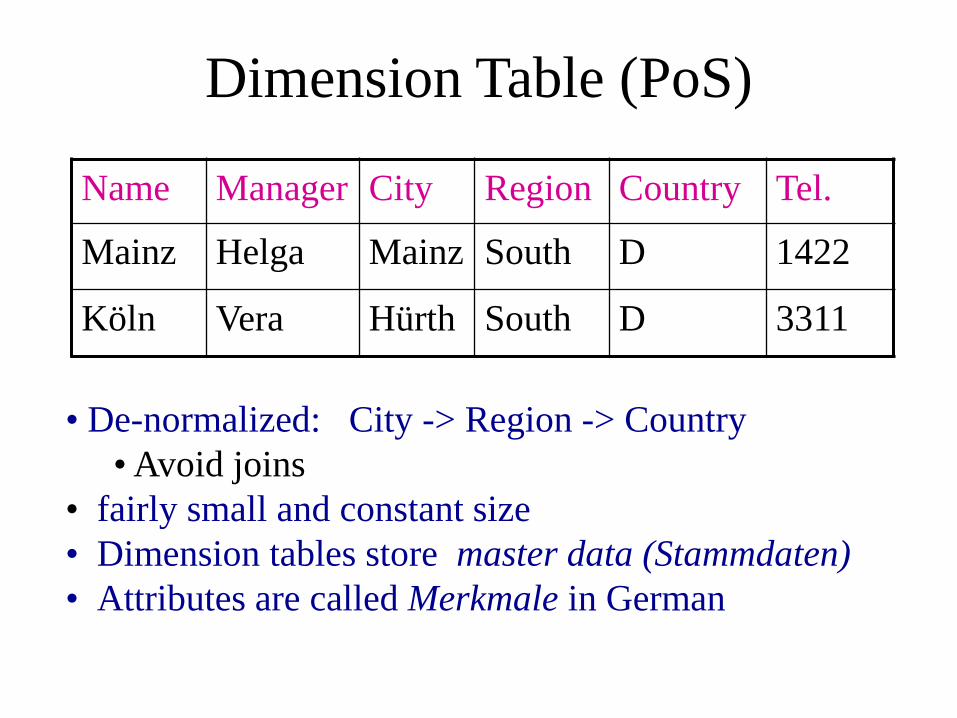
Dimension Table (PoS)

Name Manager City Region Country Tel.

Mainz Helga Mainz South D 1422

Köln Vera Hürth South D 3311

• De-normalized: City -> Region -> Country

• Avoid joins

• fairly small and constant size

• Dimension tables store master data (Stammdaten)

• Attributes are called Merkmale in German

Snowflake Schema

• If dimension tables get too large

– Partition the dimension table

• Trade-Off

– Less redundancy (smaller tables)

– Additional joins needed

• Exercise: Do the math!

Typical Queries

• Select by Attributes of Dimensions

– E.g., region = „south“

• Group by Attributes of Dimensions

– E.g., region, month, quarter

• Aggregate on measures

– E.g., sum(price * volumen)

SELECT d1.x, d2.y, d3.z, sum(f.z1), avg(f.z2)

FROM Fact f, Dim1 d1, Dim2 d2, Dim3 d3

WHERE a < d1.feld < b AND d2.feld = c AND

Join predicates

GROUP BY d1.x, d2.y, d3.z;

Example

SELECT f.region, z.month, sum(a.price * a.volume)

FROM Order a, Time z, PoS f

WHERE a.pos = f.name AND a.date = z.date

GROUP BY f.region, z.month

South May 2500

North June 1200

South October 5200

North October 600

Star Schema vs. Big Data

• Star Schema designed for specific questions – define “metrics” and “dimensions” upfront

– thus, define questions you can ask upfront

– great for operational BI

– bad for ad-hoc questions (e.g., disasters)

– breaks philosophy of Big Data (collect, then think) • e.g., health record: is “disease” metric or dimension?

• Poor on diversity – even if you know all the questions upfront, you may

end up with multiple Star schemas

Drill-Down und Roll-Up

• Add attribute to GROUP BY clause

– More detailed results (e.g., more fine-grained results)

• Remove attribute from GROUP BY clause

– More coarse-grained results (e.g., big picture)

• GUIs allow „Navigation“ through Results

– Drill-Down: more detailed results

– Roll-Up: less detailed results

• Typical operation, drill-down along hierarchy:

– E.g., use „city“ instead of „region“

Data Cube

Product

Region

Year

all North South

all

Balls

Nets 1998

1999 2000

alle

Sales by Product and

Year

Moving Sums, ROLLUP

• Example: GROUP BY ROLLUP(country, region, city) Give totals for all countries and regions

• This can be done by using the ROLLUP Operator

• Attention: The order of dimensions in the GROUP

BY clause matters!!!

• Again: Spreadsheets (EXCEL) are good at this

• The result is a table! (Completeness of rel. model!)

ROLLUP alla IBM UDB

SELECT Country, Region, City, sum(price*vol)

FROM Orders a, PoS f

WHERE a.pos = f.name

GROUP BY ROLLUP(Country, Region, City)

ORDER BY Country, Region, City;

Also works for other aggregate functions; e.g., avg().

Result of ROLLUP Operator

D North Köln 1000

D North (null) 1000

D South Mainz 3000

D South München 200

D South (null) 3200

D (null) (null) 4200

Summarizability (Unit)

• Legal Query SELECT product, customer, unit, sum(volume) FROM Order GROUP BY product, customer, unit;

• Legal Query (product -> unit) SELECT product, customer, sum(volume) FROM Order GROUP BY product, customer;

• Illegal Query (add „kg“ to „m“)!!! SELECT customer, sum(volume) FROM Order GROUP BY customer;

Summarizability (de-normalized data)

Region Customer Product Volume Populat.

South Heinz Balls 1000 3 Mio.

South Heinz Nets 500 3 Mio.

South Mary Balls 800 3 Mio.

South Mary Nets 700 3 Mio.

North Heinz Balls 1000 20 Mio.

North Heinz Nets 500 20 Mio.

North Mary Balls 800 20 Mio.

North Mary Nets 700 20 Mio.

Customer, Product -> Revenue

Region -> Population

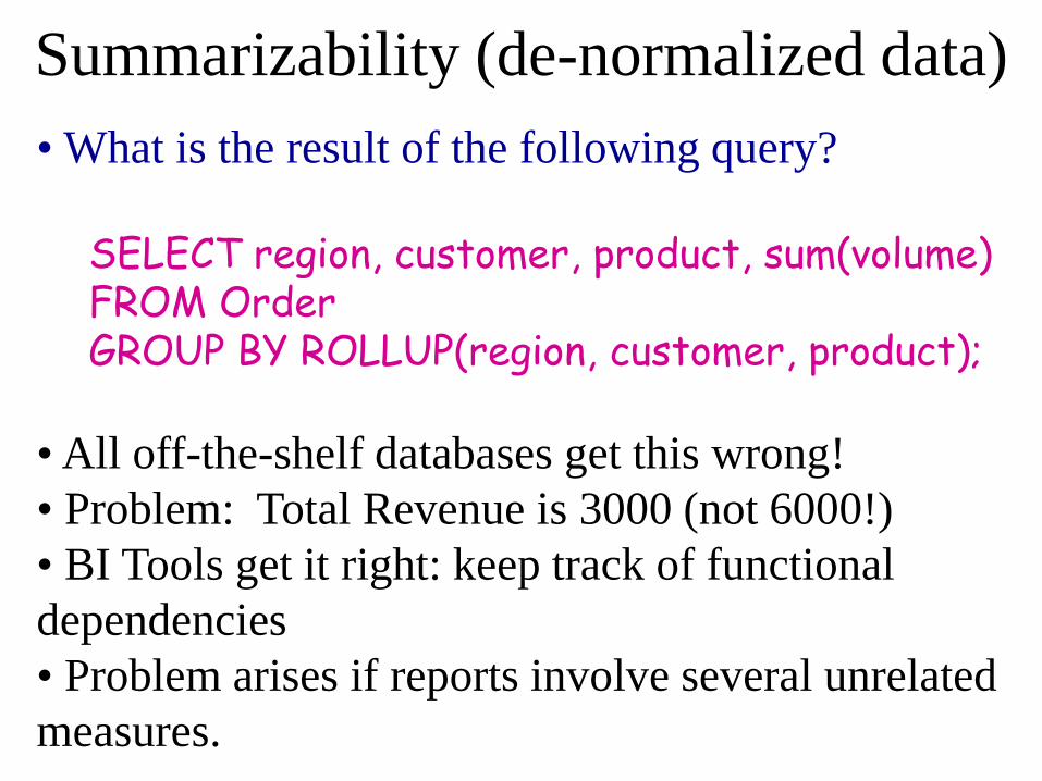
Summarizability (de-normalized data)

• What is the result of the following query?

SELECT region, customer, product, sum(volume) FROM Order GROUP BY ROLLUP(region, customer, product);

• All off-the-shelf databases get this wrong!

• Problem: Total Revenue is 3000 (not 6000!)

• BI Tools get it right: keep track of functional

dependencies

• Problem arises if reports involve several unrelated

measures.

Overview

• Motivation and Architecture

• SQL Extensions for Data Warehousing (DSS)

– Algorithms and Query Processing Techniques

• Column Stores, Vector Databases

• Parallel Databases

• Operational BI

Cube Operator

• Operator that computes all „combinations“

• Result contains „(null)“ Values to encode „all“

SELECT product, year, region, sum(price * vol)

FROM Orders

GROUP BY CUBE(product, year, region);

Result of Cube Operator

Product Region Year Revenue

Netze Nord 1998 ...

Bälle Nord 1998 ...

(null) Nord 1998 ...

Netze Süd 1998 ...

Bälle Süd 1998 ...

(null) Süd 1998 ...

Netze (null) 1998 ...

Bälle (null) 1998 ...

(null) (null) 1998 ...

Visualization as Cube

Product

Region

Year

all North South

all

Balls

Nets 1998

1999 2000

all

Computation Graph of Cube

{product, year, region}

{product}

{product, region} {year, region} {product, year}

{year} {region}

{}

Pivot Tables

• Define „columns“ by group by predicates • Not a SQL standard! But common in products •Reference:

• Cunningham, Graefe, Galindo-Legaria: PIVOT and UNPIVOT: Optimization and Execution Strategies in an RDBMS. VLDB 2004

Materialized Views

• Compute the result of a query using the result

of another query

• Principle: Subsumption

– The set of all German researchers is a subset of the

set of all researchers

– If query asks for German researchers, use set of all

researchers, rather than all people

• Subsumption works well for GROUP BY

Materialized View

SELECT product, year, region, sum(price * vol) FROM Order GROUP BY product, year, region;

SELECT product, year, sum(price * vol) FROM Order GROUP BY product, year;

Materialized View GROUP BY

product, year

Optimization of Group Bys

• Give each department with salary of employees SELECT e.dno, d.budget, sum(e.salary) FROM Emp e, Dept d WHERE e.dno = d.dno GROUP BY e.dno, d.budget;

• Plan 1: Join before Group By (classic)

– G(Emp 1 Dept)

• Plan 2: Join after Group By (advanced)

– G(Emp) 1 Dept

• Assessment

– Why (or when) is Plan 2 legal?

– Why (or when) is Plan 1 better than Plan 2?

UNPIVOT (material, factory)

PIVOT (material, factory)

Top N

• Many applications require top N queries

• Example 1 - Web databases

– find the five cheapest hotels in Madison

• Example 2 - Decision Support

– find the three best selling products

– average salary of the 10,000 best paid employees

– send the five worst batters to the minors

• Example 3 - Multimedia / Text databases

– find 10 documents about „database“ and „web“.

• Queries and updates, any N, all kinds of data

Key Observation

• So what do you do?

– Implement top N functionality in your application

– Extend SQL and the database management system

Top N queries cannot be expressed well in SQL

SELECT * FROM Hotels h WHERE city = Madison AND 5 > (SELECT count(*) FROM Hotels h1 WHERE city = Madison AND h1.price < h.price);

Implementation of Top N in the App

• Applications use SQL to get as close as possible

• Get results ordered, consume only N objects

and/or specify predicate to limit # of results

– either too many results, poor performance

– or not enough results, user must ask query again

– difficult for nested top N queries and updates

SELECT * FROM Hotels WHERE city = Madison ORDER BY price;

SELECT * FROM Hotels WHERE city = Madison AND price < 70;

Extend SQL and DBMS

• STOP AFTER clause specifies number of results

• Returns five hotels (plus ties)

• Challenge: extend query processor, performance

SELECT * FROM Hotels WHERE city = Madison ORDER BY price STOP AFTER 5 [WITH TIES];

Updates

• Give top 5 salesperson a 50% salary raise

UPDATE Salesperson SET salary = 1.5 * salary WHERE id IN (SELECT id FROM Salesperson ORDER BY turnover DESC STOP AFTER 5);

Nested Queries

• The average salary of the top 10000 Emps

SELECT AVG(salary) FROM (SELECT salary FROM Emp ORDER BY salary DESC STOP AFTER 10000);

Extend SQL and DBMSs

• SQL syntax extension needed

• All major database vendors do it

• Unfortunately, everybody uses a different syntax

– Microsoft: set rowcount N

– IBM DB2: fetch first N rows only

– Oracle: rownum < N predicate

– SAP R/3: first N

• Challenge: extend query processor of a DBMS

Top N Queries Revisited

• Example: The five cheapest hotels

SELECT * FROM Hotels ORDER BY price STOP AFTER 5;

• What happens if you have several criteria?

Nearest Neighbor Search

• Cheap and close to the beach SELECT * FROM Hotels ORDER BY distance * x + price * y STOP AFTER 5;

• How to set x and y ?

Query Processing 101 SELECT * FROM Hotels h, Cities c WHERE h.city = c.name;

Parser &

Query Optimizer

<Ritz, Paris, ...> <Weisser Hase, Passau, ...> <Edgewater, Madison, ...>

Scan(Hotels)

Hash Join

Scan(Cities)

Execution Engine

plan

Catalogue Indexes & Base Data

Schema info, DB statistics

<Ritz, ...> ...

<Paris, ...> ...

57

Processing Top N Queries

• Overall goal: avoid wasted work

• Stop operators encapsulate top N operation

– implementation of other operators not changed

• Extend optimizer to produce plans with Stop

SELECT * FROM Hotels h, Cities c WHERE h.city = c.name ORDER BY h.price STOP AFTER 10; Hotels Cities

Join

Sort

Stop(10)

?

58

Implementation of Stop Operators

• Several alternative ways to implement Stop

• Performance depends on:

– N

– availability of indexes

– size of available main memory

– properties of other operations in the query

59

Implementation Variants

• Stop after a Sort (trivial)

• Priority queue – build main memory priority queue with first N

objects of input

– read other objects one at a time: test membership bounds & replace

• Partition the input (range-based braking)

• Stop after an Index-Scan

60

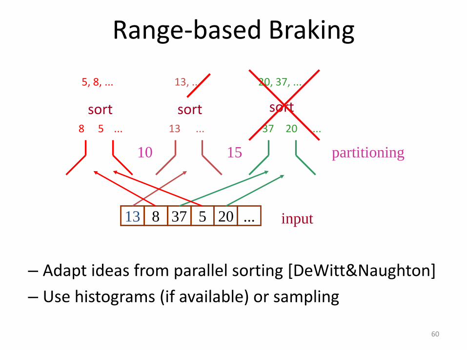
Range-based Braking

– Adapt ideas from parallel sorting [DeWitt&Naughton]

– Use histograms (if available) or sampling

13 8 37 5 20 ... input

partitioning 10 15

sort sort sort

8 5 ... 13 ... 37 20 ...

5, 8, ... 13, ... 20, 37, ...

61

Range-based Braking Variants

Input

scan

scan restart

Input

1. Materialize: store all partitions on disk

2. Reread: scan input for each partition

filter restart

3. Hybrid: materialize first x partitions; reread others

stop

stop sort

sort

sort scan

scan filter

62

Performance of Stop Operators N highest paid Emps; AODB/Sun; 4 MB mem.; 50 MB DB

N 10 100 50K ALL

Sort 104.2 103.2 112.2 117.9

PQ 54.0 52.7 n.a.n n.a.n

Mat 75.3 75.0 83.6 120.1

Reread 50.0 50.1 83.6 120.1

Hybrid 49.5 50.0 87.6 126.4

63

Stop & Indexes

• Read and follow pointers from index until N results have been produced

• Very simple to implement, result is sorted

• Random I/O if N is large or if there is an additional predicate (e.g., hotels in Madison)

5 8 13 20 37 ...

F,5

C,8

A,13 ...

output

Idxscan

Stop(N)

Fetch

A,13 C,8 D,37 F,5 H,20 ...

64

Range-based Braking & Indexes

• read first partition

• sort pointers to avoid random I/O

• read objects using (sorted) pointers

• re-sort tuples

• repeat until N results are produced

5 8 13 20 37 ...

idxscan

Stop(k)

Sort(ptr)

Fetch

Restart

Stop(N)

Sort($) A,13 C,8 D,37 F,5 H,20 ...

65

Performance Evaluation (Index) N highest paid Emps; AODB/Sun; 4 MB mem.; 50 MB DB

N 10 1K 10K 50K

Index 1.8 92.8 807.4 4505.5

Part&Index 1.0 7.8 31.0 148.1

Hybrid 49.5 55.0 55.7 87.6

66

Optimizing Top N Queries • Traditional optimizer must decide

– join order

– access paths (i.e., use of indexes), ...

• Top N optimizer must in addition decide

– which implementation of Stop operator to use

– where in a plan to place Stop operators

• Optimizer enumerates all alternative plans and selects best plan using a cost model

• Stop operators affect other decisions (e.g., join order, access paths)

67

Favor Pipelined Plans for Small N

• pipelining operators process a tuple at a time

• blocking operators consume whole input

idxscan

(hotels)

NL Join

Stop

scan

(cities) scan

(hotels)

Hash Join

Stop/PQ

scan

(cities)

5, 8, 13, 20, 37, ...

5

5

5

8 13

13

13

13, 8, 37, 5, 20, ...

13,8,37,...

13,5,,...

5 13

68

Optimization of Stop in a Pipeline

<ritz, $200>

<carlton, $100>

<plaza, $259> ...

Priority Queue

Scan(hotels)

Pipelined Ops

(e.g. filter, NLJ)

<YMCA, $25>

<Motel 5, $49>

<Days Inn, $45>

bound: $49

69

Push Down Stop Operators Through Pipeline Breakers

• Sometimes, pipelined plan is not attractive

• Or, pipelined plan is not possible (no indexes)

• In these cases, apply Stop as early as possible in order to reduce size of intermediate results

• Analogous to predicate push-down in traditional query optimization

70

Conservative Approach • example:

SELECT * FROM Hotels h, Cities c WHERE h.city = c.name ORDER BY price STOP AFTER 10;

• look at integrity constraints

• Push-down through non-reductive operators

• Every hotel qualifies join (join is non-reductive)

hotels

Hash Join

Stop(10) cities

Stop(10)

• Stop at the top necessary

if a hotel matches several cities

71

Aggressive Approach

• Conservative approach not always applicable

• example: SELECT * FROM Hotels h, Cities c WHERE h.city = c.name AND c.state = Wisconsin ORDER BY price STOP AFTER 10;

• partition on price before join

• use DB statistics

hotels

Hash Join

Stop(50) filter

Stop(10)

Restart(10)

cities

72

Conservative vs. Aggressive

• If Conservative applicable, do it.

• Aggressive:

– can reduce the cost of other operations significantly (e.g., joins, sorts)

– (unanticipated) restarts due to poor partitioning (i.e., bad statistics) cause additional costs

• Conservative is being implemented by IBM

• No commercial product is Aggressive yet

73

Union Queries (Parallel System)

SELECT * FROM Hotels ORDER BY price STOP AFTER 10; UNION

Hotels 1

Stop(10)

Hotels 2

Stop(10)

Hotels 3

Stop(10)

Stop(10)

Client

Server 1 Server 2 Server 3

74

Top N and Semi-joins

• Idea – keep rids, project out columns at the beginning

– at the end use rids to refetch columns

• Tradeoff – reduces cost of joins, sorts etc. because

intermediate results are smaller

– additional overhead to refetch columns

• Attractive for top N because N limits refetch

Skyline Queries

• Hotels which are close to the beach and cheap.

distance

price

x x

x x

x

x x x x

x

x

x

x

x

x x

x x

Top 5 Skyline (Pareto Curve)

x x

x

Convex Hull

Literatur: Maximum Vector Problem. [Kung et al. 1975]

Syntax of Skyline Queries

• Additional SKYLINE OF clause [Börszönyi, Kossmann, Stocker 2001]

• Cheap & close to the beach SELECT * FROM Hotels WHERE city = ´Nassau´ SKYLINE OF distance MIN, price MIN;

Flight Reservation

• Book flight from Washington DC to San Jose

SELECT * FROM Flights WHERE depDate < ´Nov-13´ SKYLINE OF price MIN, distance(27750, dept) MIN, distance(94000, arr) MIN, (`Nov-13` - depDate) MIN;

Visualisation (VR)

• Skyline of NY (visible buildings)

SELECT * FROM Buildings WHERE city = `New York` SKYLINE OF h MAX, x DIFF, z MIN;

Location-based Services

• Cheap Italian restaurants that are close

• Query with current location as parameter

SELECT * FROM Restaurants WHERE type = `Italian` SKYLINE OF price MIN, d(addr, ?) MIN;

Skyline and Standard SQL

• Skyline can be expressed as nested Queries

SELECT * FROM Hotels h WHERE NOT EXISTS ( SELECT * FROM Hotels WHERE h.price >= price AND h.d >= d AND (h.price > price OR h.d > d))

• Such queries are quite frequent in practice

• The response time is desastrous

Naive Algorithm

• Nested Loops

– compare every point with every other point

FOR i=1 TO N D = FALSE; j = 1; WHILE (NOT D) AND (j <= N) D = dominate(a[j], a[i]); j++; END WHILE IF (NOT D) output(a[i]); END FOR

Block Nested-Loops Algorithm

• Problems of naive algorithm

– N scans of entire table

• (many I/Os if table does not fit in memory

– points are compared twice

• Block Nested Loops Algorithm

– keep window of uncomparable points

– demote points not in window into temp file

• Assessment

– N / windowsize scans through DB

– no pairs of points are every compared twice

BNL Exampe

Input: ABCDEFG

Windowsize = 2

A

y

x

D B

C F

E G

Step Window Input Temp Output

1,2 AB CDEFG

3 AC DEFG

4-7 AC EFG

8 EFG AC

9-11 EG AC

12 ACEG

BNL Variants

• „Self-organizing List“

– move hits to the beginning of window

– saves CPU cost for comparisons

• „Replacement“

– maximize „volume“ of window

– additional CPU overhead

– less iterations because more effective window

Divide & Conquer Algorithm

• [Kung et al. 1975]

• Approach:

– Partition the table into two sets

– apply algo recursively to both sets

– Merge the two sets; special trick when merge

• Best algorithm in „worst case“ O(n * (log n) (d-2) )

• Poor in best case (and expected case)

• Bad if DB does not fit in main memory

Variants of D&C Algos

• M-way Partitioning

– Partition into M sets (rather than 2)

• choose M so that results fit in main memory

– Extend Merge Algorithm to M-way merge

– Optimize „Merge Tree“

– Much better I/O behavior

• Early Skyline

– Eliminate points „on-the-fly“

– saves both IO and CPU cost

2-D Skyline

1. Sort points according to “x, y”

2. Compare point only with previous point

x

y

1

3

2

4

5

7

6

8

Online Algorithms

• Return first results immediately

– Give response time guarantees for first x points

• Incremental Evaluation

– get better „big picture“ the longer the algo runs

– generate full Skyline if runs long enough

• Fairness; User controls where to invest

• Correct – never return non-Skyline points

• General, can be integrated well into DBMS

Online Skyline Algorithmus [Kossmann, Ramsak, Rost 2002]

• Divide & Conquer Algorithmus

– Look for Nearest Neighbor (e.g., using R* Baum)

– Partition space into Bounding Boxes

– Look for Nearest Neighbors in Bounding Boxes

Online Skyline Algorithmus [Kossmann, Ramsak, Rost 2002]

• Divide & Conquer Algorithmus

– Look for Nearest Neighbor (e.g., using R* Baum)

– Partition space into Bounding Boxes

– Look for Nearest Neighbors in Bounding Boxes

• Correctness - 2 Lemmas

– Every Nearest Neighbor is a Skyline point

– Every Nearest Neighbor in a Bounding Box is a Skyline point

Der NN Algorithmus

distance

price

x

x

x x

x x

x

x

x

x

x x

x x x

x x

Der NN Algorithmus

distance

price

x

x

x x

x x

x

x

x

x

x x

x x x

x x

Der NN Algorithmus

distance

price

x

x

x x

x x

x

x

x

x

x x

x x x

x x

Der NN Algorithmus

distance

price

x

x

x x

x x

x

x

x

x

x x

x x x

x x

Der NN Algorithmus

distance

price

x

x

x x

x x

x

x

x

x

x x

x x x

x x

x

x

x

x

x

Der NN Algorithmus

distance

price

x

x

x x

x x

x

x

x

x

x x

x x x

x x

x

x

x

x

x

Implementierung

• NN Search with R* Tree, UB Tree, ...

– Bounding Boxes easy to take into account

– Other predicates easy to take into account

– Efficient and highly optimized in most DBMS

• For d > 2 bounding boxes overlap

– need to eliminate duplicates

– Merge Bounding Boxes

– Propagate NNs

• Algorithm works well for mobile applications

– Parameterized search in R* Tree

Experimentelle Bewertung

M-way D&C

NN (prop) NN (hybrid)

User Control

distance

price

x

x

x x

x x

x

x

x

x

x x

x x x

x x

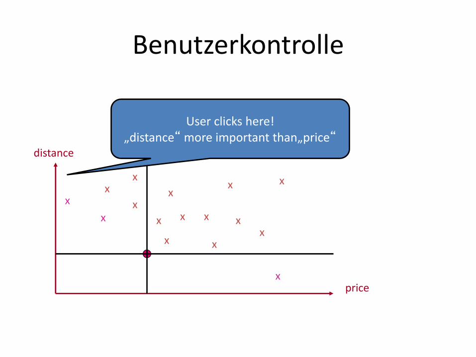
Benutzerkontrolle

distance

price

x

x

x x

x x

x

x

x

x

x x

x x x

x x

User clicks here! „distance“ more important than„price“

User Control

distance

price

x

x

x x

x x

x

x

x

x

x x

x x x

x x

User Control

distance

price

x

x

x x

x x

x

x

x

x

x x

x x x

x x

Online Aggregation

• Get approximate result very quickly

• Result (conf. intervals) get better over time

• Based on random sampling (difficult!)

• No product supports this yet

SELECT cust, avg(price) FROM Order GROUP BY cust

Cust Avg +/- Conf

Heinz 1375 5% 90%

Ute 2000 5% 90%

Karin - - -

Time

• There are two kinds of times – application specific; e.g., order date, shipping date

– system specific; when did order enter system

– bi-temporal data model

• System time can be simulated in App – but cumbersome

– most systems have built-in features for System time

• There is no update – only a new version of data – supports application-defined UNDO

– (you can spend a whole lecture on this!)

Time Travel

• Give results of query AS OF a certain point in time

• Idea: Database is a sequence of states

– DB1, DB2, DB3, … DBn

– Each commit of a transaction creates a new state

– To each state, associate time stamp and version number

• Idea builds on top of „serialization“

– Time travel mostly relevant for OLTP system in order to get reproducable results or recover old data

• Implementation (Oracle - Flashback)

– Leverage versioned data store + snapshot semantics

– Chaining of versions of records

– Specialized index structures (add time as a „parameter“)

Time Travel Syntax

• Give me avg(price) per customer as of last week

SELECT cust, avg(price)

FROM Order AS OF MAR-23-2007

GROUP BY cust

• Can use timestamp or version number

– Special built-in functions to convert timestamp <-> von

– None of this is standardized (all Oracle specific)

• Now Temporal Join and Temporal Aggregation

Notification (Oracle)

• Inform me when account drops below 1000

SELECT * FROM accounts a WHEN a.balance < 1000

• Based on temporal model

– Query state transitions; monitor transition: false->true

– No notification if account stays below 1000

• Some issues:

– How to model „delete“?

– How to create an RSS / XML stream of events?

DBMS for Data Warehouses

• ROLAP – Extend RDBMS

– Special Star-Join Techniques

– Bitmap Indexes

– Partition Data by Time (Bulk Delete)

– Materialized Views

• MOLAP – special multi-dimensional systems

– Implement cube as (multi-dim.) array

– Pro: potentially fast (random access in array)

– Problem: array is very sparse

• Religious war (ROLAP wins in industry)

Overview

• Motivation and Architecture

• SQL Extensions for Data Warehousing (DSS)

– Algorithms and Query Processing Techniques

• Column Stores, Vector Databases

• Parallel Databases

• Operational BI

A B C D E F

A B

C D

E F

OLA

P

OLTP

Row Store vs. Column Store

• OLTP: many inserts of new rows • OLAP: read (few) whole columns

• denormalization adds to this observation

Advantages of Column Stores

• Data Locality – you only read the data that you need

– you only buffer the data that you need

– small intermediate results (“position lists”)

– true for disk-based & in-memory systems

• Compression – lower entropy within a column than row

– (again, important for disk-based & in-memory)

• SIMD Instructions – execute same operation on several values at once

– (e.g., 64 bit machine with 32 bit integers -> x2)

Query Processing in Column Stores

SELECT sum(price) FROM Order WHERE product=“ball”;

RowID Product

1 ball

2 net

3 ball

4 ball

5 racket

6 net

RowID

1

3

4

RowID Price

1 5

2 10

3 7

4 9

5 12

6 2

s 1 RowID Price

1 5

3 7

4 9

=

Psum

sum

21

Disadvantages of Column Stores

• Every query involves a join of the columns – cheap if you keep position lists sorted

– not a problem if you always scan anyway • (more on that later)

• Need to “materialize” tuples; copy data – not a problem for aggregate queries (small results)

– not a problem if round-trips to disk needed

– optimizer controls best moment to “materialize”

• Every insert involves n inserts (n columns) – that is why not good for OLTP!!!

Vectorization • Iterator Model (-> Bachelor courses)

– open() – next() – close() Interface of operators

– next() returns (pointer to) one result tuple

– great for composability of operators

– great for pipelined parallelism

• Problems of Iterator Model

– poor instruction cache locality

• reload code of every operator with every tuple

– poor use of bandwidth of “bus” (network in machine)

• ship 32 bit pointers on 128 bit bus

• Idea: Ship batches of tuples with every next() call

– works well in row and column store

Overview

• Motivation and Architecture

• SQL Extensions for Data Warehousing (DSS)

– Algorithms and Query Processing Techniques

• Column Stores, Vector Databases

• Parallel Databases

• Operational BI

Parallel Database Systems

• Why is a query slow?

– bottlenecks

– it needs to do a lot of work

– (performance bugs; e.g., wrong plan)

• How to make it fast, if it is just a lot of work?

– partitioning and replication

– exploit different forms of parallelism

• Reference: DeWitt, Gray: CACM 1992

Why are response times long?

• Because operations take long

– cannot travel faster than light

– delays even in „single-user“ mode

– fix: parallelize long-running operations

• data partioning for „intra-query parallelism“

• Because there is a bottleneck

– contention of concurrent requests on a resource

– requests wait in queue before resource available

– add resources to parallelize requests at bottleneck

• replication for „inter-query parallelism“

Forms of Parallelism

• Inter-request Parallelism – several requests handled at the same time

– principle: replicate resources

– e.g., ATMs

• (Independent) Intra-request Parallelism – principle: divide & conquer

– e.g., print pieces of document on several printers

• Pipelining – each „item“ is processed by several resources

– process „items“ at different resources in parallel

– can lead to both inter- & intra-request parallelism

Inter-request Parallelism

Req 1

Resp. 1 Resp. 2 Resp. 3

Independent Parallelism Req 1

Req 1.1

split

Req 1.2 Req 1.3

Res 1.1 Res 1.2 Res 1.3

merge

Response 1

Pipelining (Intra-request) Req 1

split

Req 1.1

merge

Response 1

Example: Dish Washing

Speed-up

• Metric for intra-request parallelization

• Goal: reduce response time

– measure response time with 1 resource

– measure response time with N resources

– SpeedUp(N) = RT(1) / RT(N)

• Ideal

– SpeedUp(N) is a linear function

– can you imagine super-linear speed-ups?

Scale-up

• Goal: Scales with size of the problem

– measure response time with 1 server, unit problem

– measure response time with N servers, N units problem

– ScaleUp(N) = RT(1) / RT(N)

• Ideal

– ScaleUp(N) is a constant function (1)

– Can you imagine super scale-up?

Scale Out (transactional scale-up)

• Goal: Scale with users / jobs / transactions

– measure throughput: 1 server, k users

– measure throughput: N servers, k*N users

– ScaleOut(N) = Tput(1) / Tput(N)

• Ideal

– Scale-out should behave like Scale-Up

– (often terms are used interchangeably; but worth-while to notice the differences)

• Scale-out and down in Cloud Computing

– the ability of a system to adapt to changes in load

– often measured in $ (or at least involving cost)

Why is speed-up sub-linear? Req 1

Req 1.1

split

Req 1.2 Req 1.3

Res 1.1 Res 1.2 Res 1.3

merge

Response 1

Why is speed-up sub-linear?

• Cost for „split“ and „merge“ operation (Amdahl)

– those can be expensive operations

– try to parallelize them, too

• Interference: servers need to synchronize

– e.g., CPUs access data from same disk at same time

– shared-nothing architecture

• Skew: work not „split“ into equal-sized chunks

– e.g., some pieces much bigger than others

– keep statistics and plan better

How to split a problem?

• Cost model to split problem into „p“ pieces

Cost(p) = a * p + (b * K) / p

– a: constant overhead per piece for split & merge

– b: constant overhead per item of the problem

– K: total number of items in the problem

– cost for split and data processing may differ!!!

• Minimize this function

– simple calculus: Cost(p)‘=0; Cost(p)‘‘ > 0

p = sqrt( b * K / a)

• Do math if you can!!!

Distributed & Parallel Databases

• Distributed Databases (e.g., banks)

– partition the data

– install database nodes at different locations

– keep partitions at locations where frequently needed

– if beneficial replicate partitions / cache data

– goal: reduce communication cost

• Parallel Databases (e.g., Google)

– partition the data

– install database nodes within tightly-coupled network

– goal: speed-up by parallel queries on partitions

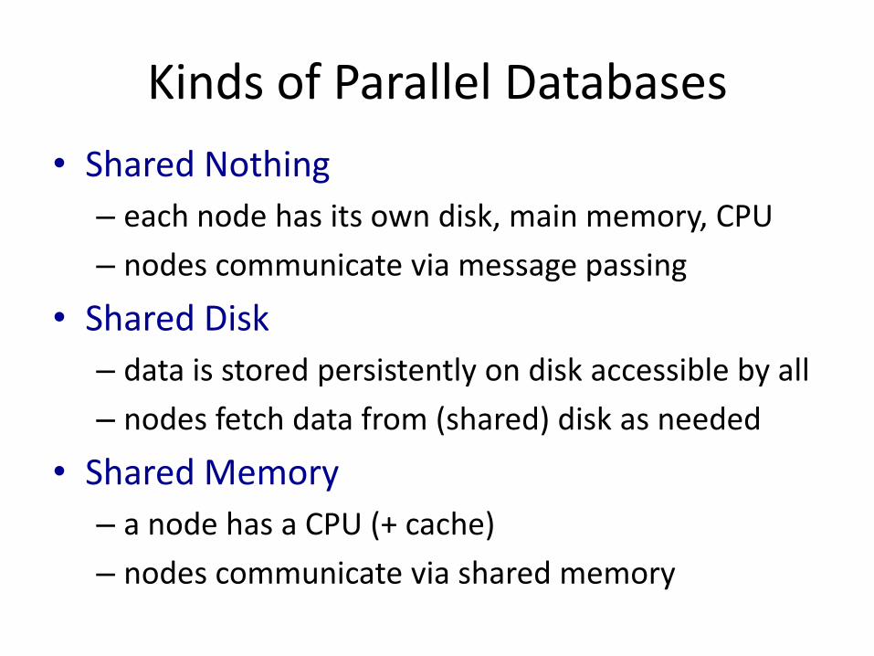
Kinds of Parallel Databases

• Shared Nothing

– each node has its own disk, main memory, CPU

– nodes communicate via message passing

• Shared Disk

– data is stored persistently on disk accessible by all

– nodes fetch data from (shared) disk as needed

• Shared Memory

– a node has a CPU (+ cache)

– nodes communicate via shared memory

Scans in Shared Nothing

• SELECT * FROM Emp WHERE salary > 1000;

(Helga, 2000) (Hubert, 150)

…

(Peter, 20) (Rhadia, 15000)

…

s s

U

Scans in Shared Nothing

• Approach

– each node has a (horizontal) partition of DB

– each node carries out scan + filter locally

– each node sends results to dedicated node

– dedicated node carries out U for final result

• Assessment

– scales almost linearly

– skew in communicating results may limit scalability

Joins in Shared Nothing (V1)

• Approach – Table 1 is horizontally partitioned across nodes

– ship (entire) Table 2 to all nodes

– carry out Pi(T1) T2 at each node

– compute U of all local joins

• Assessment – scales well if there is an efficient broadcast

– even better if Table 2 is already replicated everywhere • or if the database is shared (see later)

Joins in Shared Nothing (V2) • Approach

– partition Table 1 using Function h • ship partitions to different nodes accordingly

– partition Table 2 using Function h • ship partitions to different nodes accordingly

– carry out local joins at each node

– compute U of all local joins

• Assessment – ships both Tables entirely through network

– sensitive to skew during partitioning • can be fixed by building histograms in a separate phase

– computationally as good as hash join

Encapsulating Parallelism

T1 T2

split split

join join join join

merge

[Graefe, 1992]

Encapsulating Parallelism (Plans)

T1 T2

split split

join

merge

join join

T3

split

join join

SELECT x, y, z FROM T1, T2, T3 WHERE T1.a = T2.b AND T2.b = T3.c;

Joins in Shared Memory

• Approach

– build hash table of Table 2 in shared memory

– parallel probe hash table with Table 1

• Assessment

– resource contention on bus during probe

– build phase cannot be parallelized

– (rarely a good idea; need special HW)

Why are PDDBs so cool? ;-)

• Data is a „resource“ (just like a server)

– data can be a bottleneck if it is updated

– data can be replicated in order to improve thruput

• Data is a „problem“

– data can be partitioned in good and poor ways

– partitioning can be done statically and dynamically

– if statically, then „split“ operation is free

• Data can be used for scalability experiments

– you can nicely show all

How to partition data?

• (here: horizontal partitioning only)

• Step 1: Need to determine partitioning factor – very difficult task; depends on many factors

• Step 2: Determine partitioning method – Round-robin: good for load balancing

– Predicate-based: good for certain queries (e.g., sort)

– Hashing: good for „key“ look-ups and updates

– Sharding: partition dependent tables in the same way

• Step 3: Determine allocation – which partition to replicate and how often

– where to store replicas of each partition

Response Time Cost Models

• Estimate the response time of a query plan – Consider independent parallelism

• max

– Consider pipelined parallelism • materialized front + max

– Consider resource contention • consumption vector + max

• [Ganguly et al., 1992]

Independent Parallelism

• Response Time = max(RT(join1), RT(join2))

– assuming nothing else is happening

T1 T2

join1

T3 T4

join2

Pipelined Parallelism

max(RT(join2), RT(build1)) + max(RT(probe1), RT(probe3)

T1 T2

join1

T3 T4

join2

materialized front pipeline

join3

Resource Contention

• What if join1, join3 executed on same node?

• Model resource consumption as vector

– Consumption(probe3) = (m1, m2, m3, network)

• Add resource consumption of parallel operators

– E.g., Consumption(probe3) + Consumption (probe1)

• Model capacity as capacity vector

– Capacity = (m1, m2, m3, network)

• Match aggregated consumption with capacity

– May result in higher response times

Summary

• Improve Response Times by „partitioning“ – divide & conquer approach

– works extremely well for databases and SQL

– do the math for query optimization

• Improve Throughput by „inter-query“ parallelism – limited in SQL because of concurrency control

• Parallelism problems in databases – resource contention (e.g., lock conflicts, network)

– skew and poor load balancing

• Special kinds of experiments for scalability – speed-up and scale-up experiments

Overview

• Motivation and Architecture

• SQL Extensions for Data Warehousing (DSS)

– Algorithms and Query Processing Techniques

• Column Stores, Vector Databases

• Parallel Databases

• Operational BI

Operational BI

• Sometimes you need fresh data for decisions

– you need to be transactionally consistent

– or you cannot afford delay of ETL

• Examples

– passenger lists at airlines

– route visitors at Disney resorts

– …

Amadeus Workload • Passenger Booking Database

– ~ 600 GB of raw data (two years of bookings)

– single denormalized table (for now)

– ~ 50 attributes: flight-no, name, date, ..., many flags

• Query Workload – up to 4000 queries / second

– latency guarantees: 2 seconds

– today: only pre-canned queries allowed

• Update Workload – avg. 600 updates per second (1 update per GB per sec)

– peak of 12000 updates per second

– data freshness guarantee: 2 seconds

Amadeus Query Examples

• Simple Queries

– Print passenger list of Flight LH 4711

– Give me Hon Circle members booked Zurich to Boston

• Complex Queries

– Give me all Heathrow passengers that need special assistance (e.g., after terror warning)

• Problems with State-of-the Art

– Simple queries work only because of mat. views

• multi-month project to implement new query / process

– Complex queries do not work at all

Goals • Predictable (= constant) Performance

– independent of updates, query types, ...

• Meet SLAs – latency, data freshness

• Affordable Cost – ~ 1000 commodity servers are okay

– (compare to mainframe)

• Meet Consistency Requirements – monotonic reads and writes (ACID not needed)

• Respect Hardware Trends – main-memory, NUMA, large data centers

• Allow any kind of ad-hoc query (e.g., terror, volcano)

New Approaches for Operational BI

• Have all data in one database!

• Use a traditional DBMS with Snapshot Isolation

– SI addresses lock conflicts between OLAP + OLTP

• Delta Indexing (+ SI)

– read vs. write optimized data structures

• Crazy new ideas

– e.g. Crescando and Swissbox

Snapshot Isolation

• When a TA starts it receives a timestamp, T.

• All reads are carried out as of the DB version of T.

– Need to keep historic versions of all objects!!!

• All writes are carried out in a separate buffer.

– Writes only become visible after a commit.

• When TA commits, DBMS checks for conflicts

– Abort TA1 with timestamp T1 if exists TA2 such that

• TA2 committed after T1 and before TA1

• TA1 and TA2 updated the same object

• Snapshot Isolation and serializability? [Berenson+95]

• Advantages/disadv. of Snapshot Isolation? 151

SI and Lost Update

write(A)

commit

read(A)

T2

commit

write(A)

T1

8.

7.

6.

5.

4.

3.

2.

1.

Step

read(A)

BOT

BOT

152

SI and Lost Update (ctd.)

write(A)

commit

read(A)

T2

commit

write(A)

T1

8.

7.

6.

5.

4.

3.

2.

1.

Step

read(A)

BOT

BOT

SI reorders R1(A) and W2(A) -> not seriliz. -> abort of T1 153

SI and Uncommitted Read

write(A)

BOT

read(A)

…

T2

abort

read(B)

write(A)

BOT

T1

8.

7.

6.

5.

4.

3.

2.

1.

Step

read(A)

154

Discussion: Snapshot Isolation

• Concurrency and Availability

– No read or write of a TA is ever blocked – (Blocking only happens when a TA commits.)

• Performance – Need to keep write-set of a TA only – Very efficient way to implement aborts – Often keeping all versions of an object useful anyway – No deadlocks, but unnecessary rollbacks – Need not worry about phantoms (complicated with 2PL)

• Correctness (Serializability): Write Skew – Checking integrity constraint also happens in the

snapshot – Two concurrent TAs update different objects – Each update okay, but combination not okay – Example: Both doctors sign out… 155

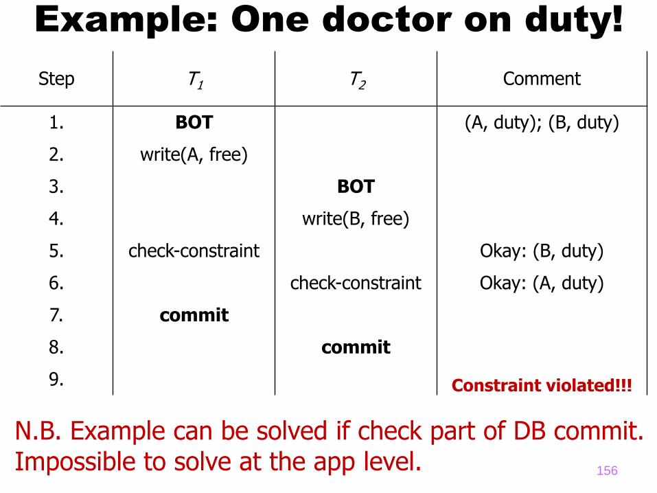
Step T1 T2 Comment

1. BOT (A, duty); (B, duty)

2. write(A, free)

3. BOT

4. write(B, free)

5. check-constraint Okay: (B, duty)

6. check-constraint Okay: (A, duty)

7. commit

8. commit

9. Constraint violated!!!

Example: One doctor on duty!

N.B. Example can be solved if check part of DB commit. Impossible to solve at the app level. 156

New Approaches for Operational BI

• Have all data in one database!

• Use a traditional DBMS with Snapshot Isolation

– SI addresses lock conflicts between OLAP + OLTP

• Delta Indexing (+ SI)

– read vs. write optimized data structures

• Crazy new ideas

– e.g. Crescando and Swissbox

Delta Indexing

• Key Idea (e.g., SAP Hana) – have a write optimized data structure (called D) – have a read optimized data structure (called “main”) – all updates create D records in D

– all queries need to be executed against D and main – periodically merge D and main so that D stays small

• Assessment – balance read and write performance,

• a number of low-level optimizations possible

– SI can nicely be integrated, allows relaxed consistency • e.g. Movies (Blunschi et al.)

– efficient merge: sort and rebuild) • but merge is potential bottleneck

Delta Indexing

put(k, value) get(k, version)

New Approaches for Operational BI

• Have all data in one database!

• Use a traditional DBMS with Snapshot Isolation

– SI addresses lock conflicts between OLAP + OLTP

• Delta Indexing (+ SI)

– read vs. write optimized data structures

• Crazy new ideas

– e.g. Crescando and Swissbox

What is Crescando?

• A distributed (relational) table: MM on NUMA

– horizontally partitioned

– distributed within and across machines

• Query / update interface

– SELECT * FROM table WHERE <any predicate>

– UPDATE table SET <anything> WHERE <any predicate>

• Some nice properties

– constant / predictable latency & data freshness

– solves the Amadeus use case

– support for Snapshot Isolation, monotonic writes

Design • Operate MM like disk in shared-nothing architect.

– Core ~ Spindle (many cores per machine & data center)

– all data kept in main memory (log to disk for recovery)

– each core scans one partition of data all the time

• Batch queries and updates: shared scans

– do trivial MQO (at scan level on system with single table)

– control read/update pattern -> no data contention

• Index queries / not data

– just as in the stream processing world

– predictable+optimizable: rebuild indexes every second

• Updates are processed before reads

Crescando on 1 Machine (N Cores)

...

Split

Scan Thread

Scan Thread

Scan Thread

Scan Thread

Scan Thread

Merge

Input Queue

(Operations)

Input Queue

(Operations)

Output Queue

(Result Tuples)

Output Queue

(Result Tuples)

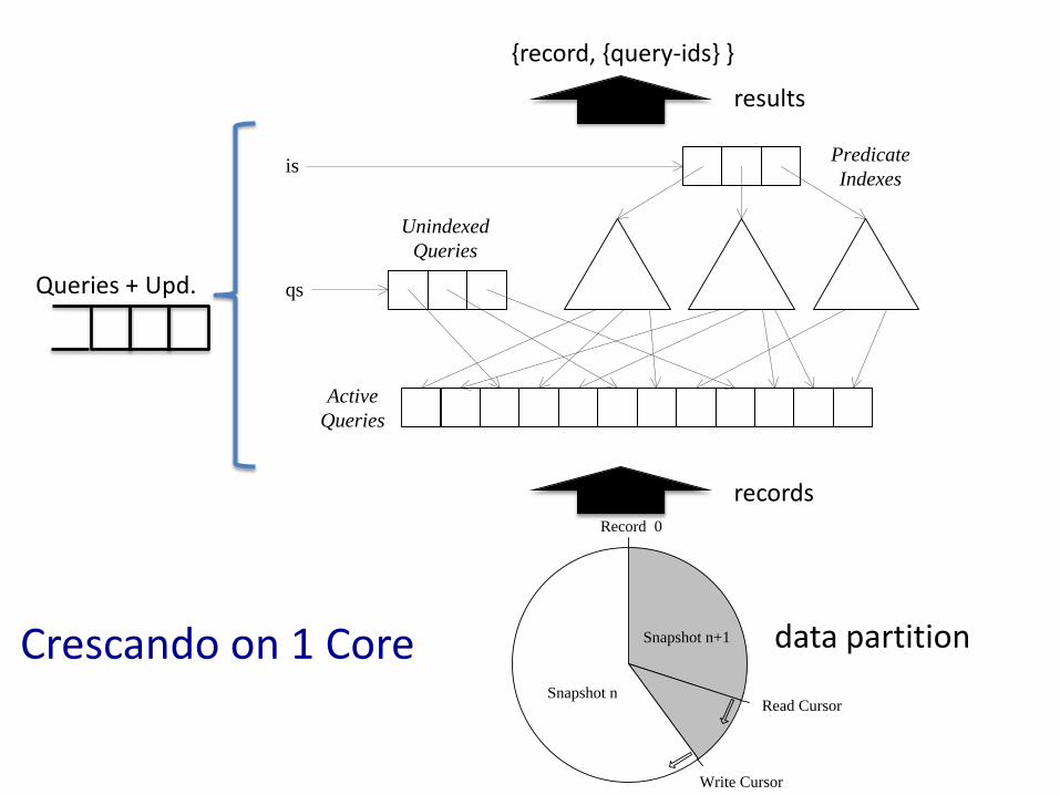
is

qs

Active

Queries

Unindexed

Queries

Predicate

Indexes

Record 0

Read Cursor

Write Cursor

Snapshot n+1

Snapshot n

Queries + Upd.

records

results

{record, {query-ids} }

Crescando on 1 Core data partition

Record 0

Read Cursor

Write Cursor

Snapshot n+1

Snapshot n

Scanning a Partition

Record 0

Read Cursor

Write Cursor

Snapshot n+1

Snapshot n

Merge cursors

Scanning a Partition

Record 0

Read Cursor

Write Cursor

Snapshot n+1

Snapshot n

Merge cursors

Build indexes for next batch of queries and updates

Scanning a Partition

Crescando @ Amadeus

Mainframe

Transactions (OLTP)

Store (e.g., S3) Store (e.g., S3) Crescando Nodes

Update stream (queue)

Aggregator Aggregator

Aggregator Aggregator

Aggregator

Queries (Oper. BI)

Key / Value

Query / {Key}

Crescando in the Cloud

Client

Store

HTTP

Web Server

App Server

DB Server

FCGI, ...

SQL

get/put block

records

XML, JSON, HTML

XML, JSON, HTML

Client Client Client

Workload Splitter

Store (e.g., S3)

Web/App Aggregator

Web/App Aggregator

XML, JSON, HTML

queries/updates <-> records

Store (e.g., S3) Crescando Nodes

Implementation Details

• Optimization – decide for batch of queries which indexes to build

– runs once every second (must be fast)

• Query + update indexes – different indexes for different kinds of predicates

– e.g., hash tables, R-trees, tries, ...

– must fit in L2 cache (better L1 cache)

• Probe indexes – Updates in right order, queries in any order

• Persistence & Recovery – Log updates / inserts to disk (not a bottleneck)

What is SharedDB?

• Implementation of relational algebra – Joins, Group-Bys, Sorting, …

• Massive sharing of operators of the same kind – Joins with the same join predicate

– Sorts with the same sorting key

• Natural extension of key Crescando idea – Apply operator on UNION of data of many queries

– Route the results to the right client

• Complements nicely with Crescando – Crescando: storage layer with predicate push-down

– SharedDB: query processor

Q1

U

R S

Q1, Q2, Q3

U

Γquery_id

σσ σ σ σσ

Q2 Q3

Q1 Q1Q2 Q2 Q3Q3

R.id = S.id &&

R.query_id =

S.query_id

SELECT *FROM R,S WHERE R.id = S.idAND R.city = ?AND S.date = ?

SELECT *FROM R,S WHERE R.id = S.idAND R.name = ?AND S.price < ?

SELECT *FROM R,S WHERE R.id = S.idAND R.address = ?AND S.date > ?

σ

R S

σ σ

R S

σ σ

R S

σQ1 Q1 Q2 Q2 Q3 Q3

R.id = S.id R.id = S.id R.id = S.id

Traditional Query Processing

Set of Queries

Shared Query Processing

Shared Group By

Shared JoinShared Duplicate

Elimination (Union)

Crescando Storage Engine

Set of Active Queries S

har

ed Q

uer

y P

roce

ssin

g E

ng

ine

Q1 Q2 Q3

Shared Sort

Global / Always-on Query Plan

Overview of Components

Take Home Messages • Big Data (Data-driven Intelligence) is not new

– 40 years of experience in database technology

– “volume” pretty much under control, unbeatable perf. (!)

– “complexity” addressed with SQL extensions

– many success stories

• What are the short-comings of data warehouses? – “diversity” – only 20% of data is relational

• very expensive to squeeze other 80% into tables

– “fast” – ETL is cumbersome and painful • in-situ processing of data much better

– “complexity” – at some point, SQL hits its limits • success kills (-> similar story with Java)

• Bottom line: Flexibility (time to market) vs. Cost