Pang eoA c o m m u n i t y - d r i v e n e f f o r t f o r

B i g D ata g e o s c i e n c e

!2

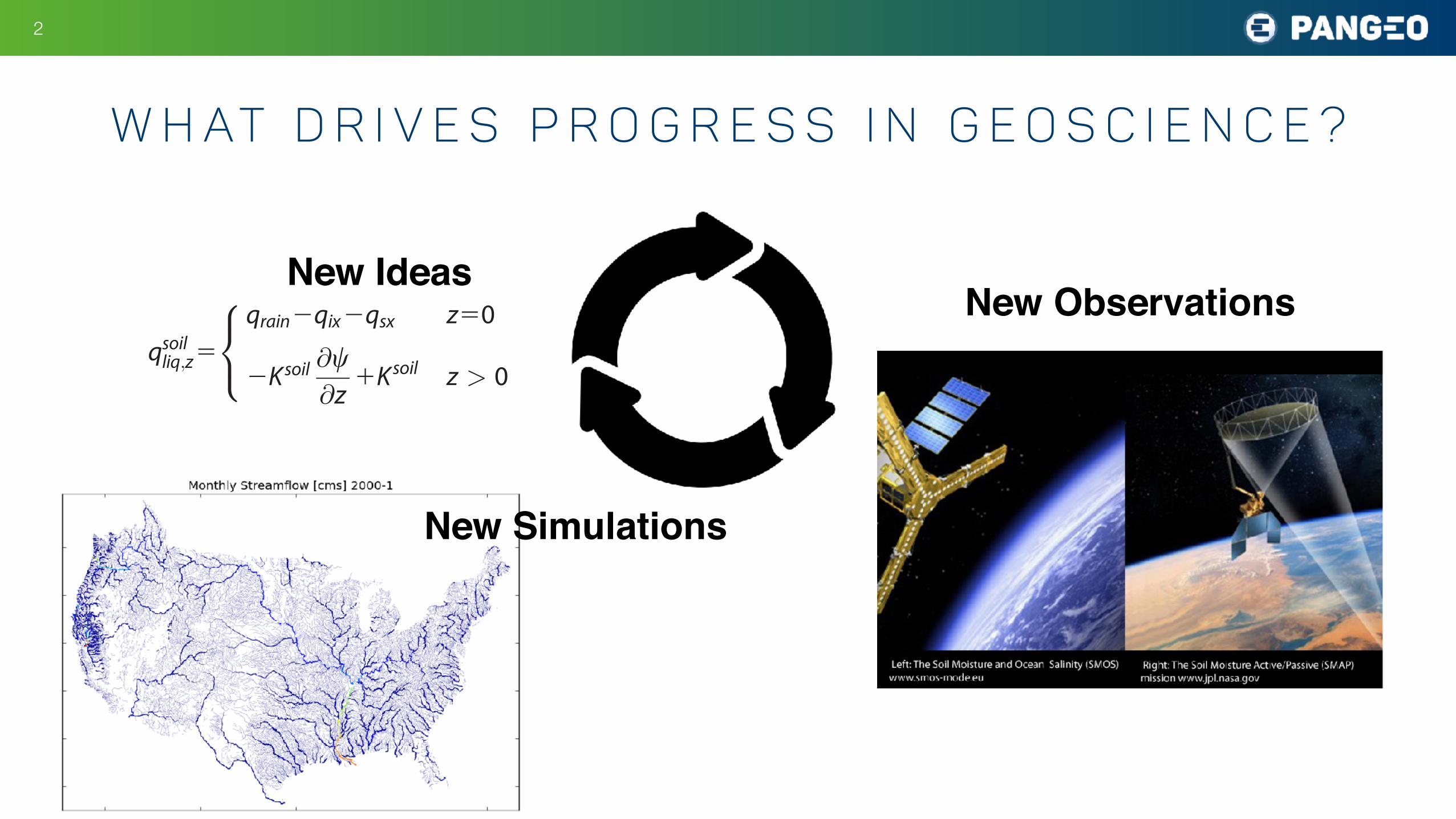
W h at D r i v e s P r o g r e s s i n G E O S c i e n c e ?

New Simulations

New ObservationsNew Ideas

snowfall over bare ground and at times when the canopy is completely covered with snow). Note that inequation (14) the solid precipitation flux occurs only at the top of the snowpack (z 5 2hsfc).

An additional equation is needed to describe the compaction of the snowpack. This is described in discre-tized form in section 4.1.4

2.2.3. Soil HydrologyThe conservation equation for soil hydrology is

@Hsoilm

@t5@qsoil

liq;x

@x1@qsoil

liq;y

@y2@qsoil

liq;z

@z1

Esoilevap1Esoil

trans

q liq(15)

In contrast to equations (12) and (13) where qice< qliq, in equation (15) we assume that qice 5 qliq, meaningthat there is no volume expansion during freezing [Dal’Amico et al., 2011], and hence Hsoil

m 5hsoilliq 1hsoil

ice .

On the RHS of equation (15), the terms qsoilliq;x , qsoil

liq;y , and qsoilliq;z (m s21) define the liquid fluxes in the x, y, and z

directions, and the terms Esoilevap and Esoil

trans (kg m23 s21) define the losses due to soil evaporation and transpi-ration, respectively.

To accommodate both unsaturated and saturated flow through soils, the fluxes on the RHS of equation (15)must be formulated as a function of liquid water matric potential, w (m). This requires additional functionsto relate the fluxes to the liquid water matric potential and to relate total water matric potential to totalwater content.

For example, the vertical fluxes of liquid water can be parameterized as a Darcy flux, with infiltration intothe soil as the upper boundary condition

qsoilliq;z5

qrain2qix2qsx z50

2K soil @w@z

1K soil z > 0

8<

: (16)

where the depth z 5 0 defines the position of the soil surface. In equation (16) qrain, qix, and qsx (m s21)define rainfall, infiltration-excess runoff and saturation-excess runoff, respectively. Within the soil profile, thetwo terms of the Darcy flux are the capillary and gravity fluxes, w (m) is the liquid water matric potential,and K soil5f ðwÞ (m s21) is the unsaturated hydraulic conductivity of soil, which varies with the liquid watermatric potential.

Water retention can be given as

Hsoilm ðw0Þ5S#ðw0Þ (17)

where S*($) is the water retention curve, e.g., the Van Genuchten [1980] function, and w0 (m) is the totalwater matric potential (note that for unfrozen conditions Hsoil

m 5hsoilliq and w0 5 w).

Liquid water flow in partially frozen soils is driven by strong capillary pressure gradients that develop as iceforms in the larger pore spaces. In this work, we follow the approach adopted by Zhao et al. [1997], in which(i) the generalized Clapeyron equation is combined with the water retention curve to separate the totalwater content Hm into the volumetric fractions of liquid water hliq and ice hice (see section 2.3.1 and Clarket al. [2015a]); and (ii) ice is treated as part of the solid matrix in order to calculate the liquid water matricpotential w. Including ice as part of the solid matrix prevents freezing-induced suction under saturated con-ditions [see also Noh et al., 2011; Painter and Karra, 2014].

Assuming that ice forms part of the solid matrix, the effective saturation of soils, Se (-) is given as

Seðw0; TÞ5 hliq2hres

hsat2hice2hres(18)

where hliq and hice can be computed from w0 and T [Clark et al., 2015a], and hsat and hres (-) define the poros-ity and residual volumetric liquid water content. Based on the ‘‘freezing equals drying’’ hypothesis (i.e., thesame constitutive functions can be used to relate hliq to w under freezing and drying conditions [Spaans

Water Resources Research 10.1002/2015WR017200

CLARK ET AL. A UNIFIED APPROACH FOR PROCESS-BASED HYDROLOGIC MODELING 6

• Familiar software ecosystem

• Data-proximate deployments

• Scalability

• Emphasis on next-generation data storage formats for the geosciences

• Demonstration

!3

R e d u c i n g T i m e t o S c i e n c e w i t h P A N G E o ( a n o u t l i n e )

!4

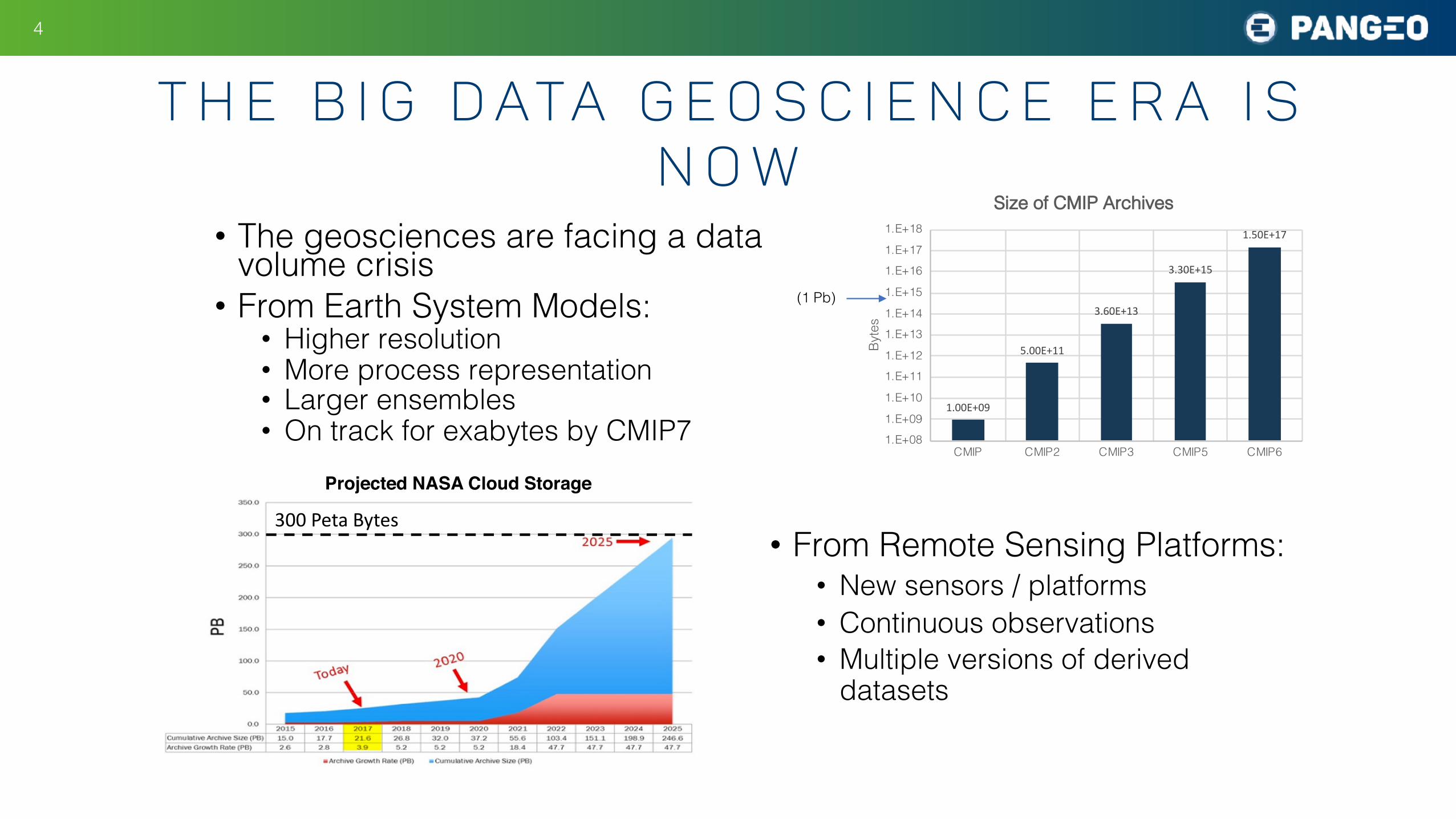
T h e b i g d ata g e o s c i e n c e e r a i s n o w

• The geosciences are facing a data volume crisis• From Earth System Models:

• Higher resolution• More process representation• Larger ensembles• On track for exabytes by CMIP7

1.00E+09

5.00E+11

3.60E+13

3.30E+15

1.50E+17

1.E+081.E+09

1.E+10

1.E+111.E+12

1.E+131.E+14

1.E+15

1.E+161.E+17

1.E+18

CMIP CMIP2 CMIP3 CMIP5 CMIP6

Byte

s

Size of CMIP Archives

Projected NASA Cloud Storage

300 Peta Bytes• From Remote Sensing Platforms:

• New sensors / platforms• Continuous observations• Multiple versions of derived

datasets

(1 Pb)

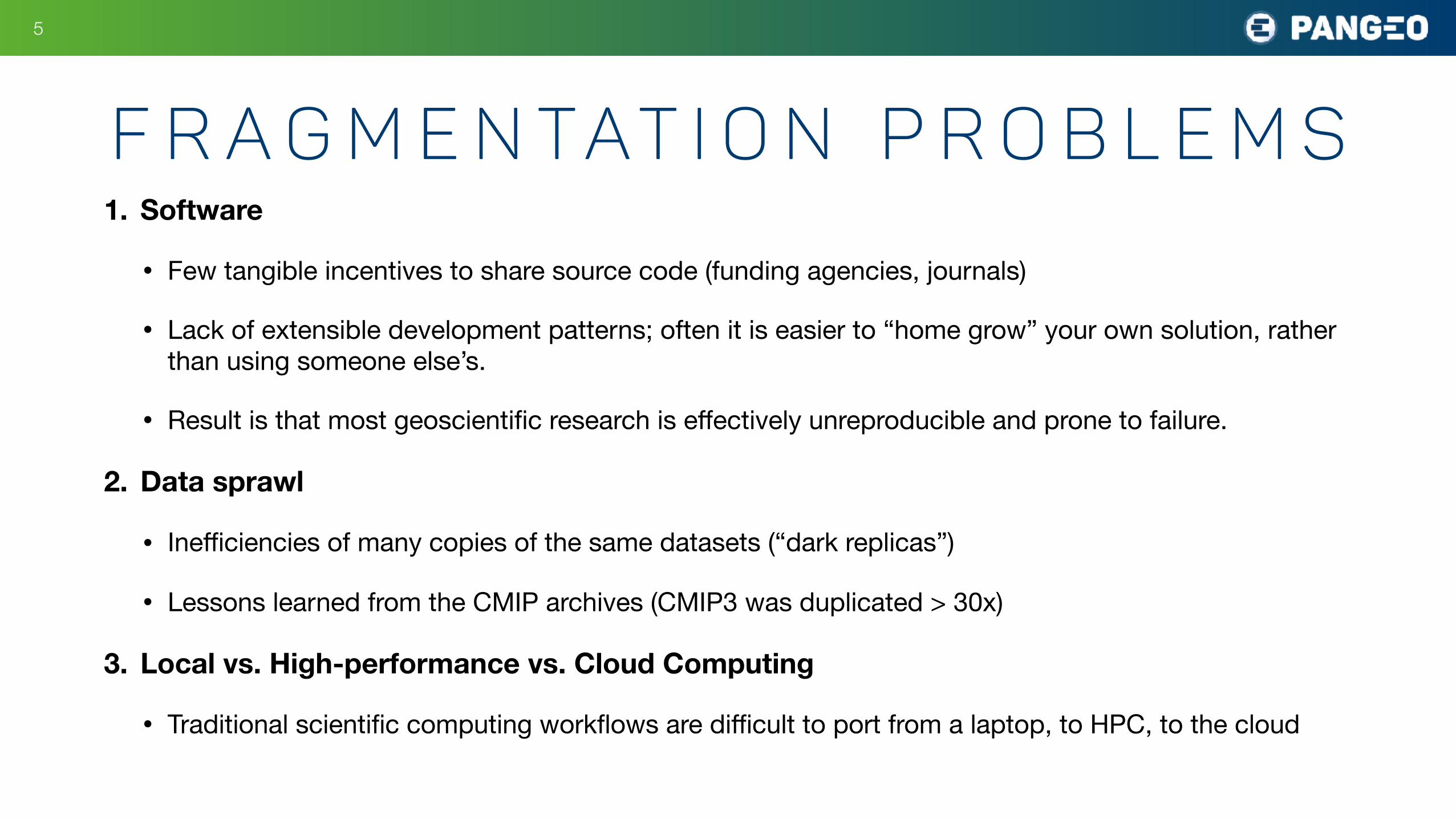
1. Software

• Few tangible incentives to share source code (funding agencies, journals)

• Lack of extensible development patterns; often it is easier to “home grow” your own solution, rather than using someone else’s.

• Result is that most geoscientific research is effectively unreproducible and prone to failure.

2. Data sprawl

• Inefficiencies of many copies of the same datasets (“dark replicas”)

• Lessons learned from the CMIP archives (CMIP3 was duplicated > 30x)

3. Local vs. High-performance vs. Cloud Computing

• Traditional scientific computing workflows are difficult to port from a laptop, to HPC, to the cloud

!5

F r a g m e n tat i o n p r o b l e m s

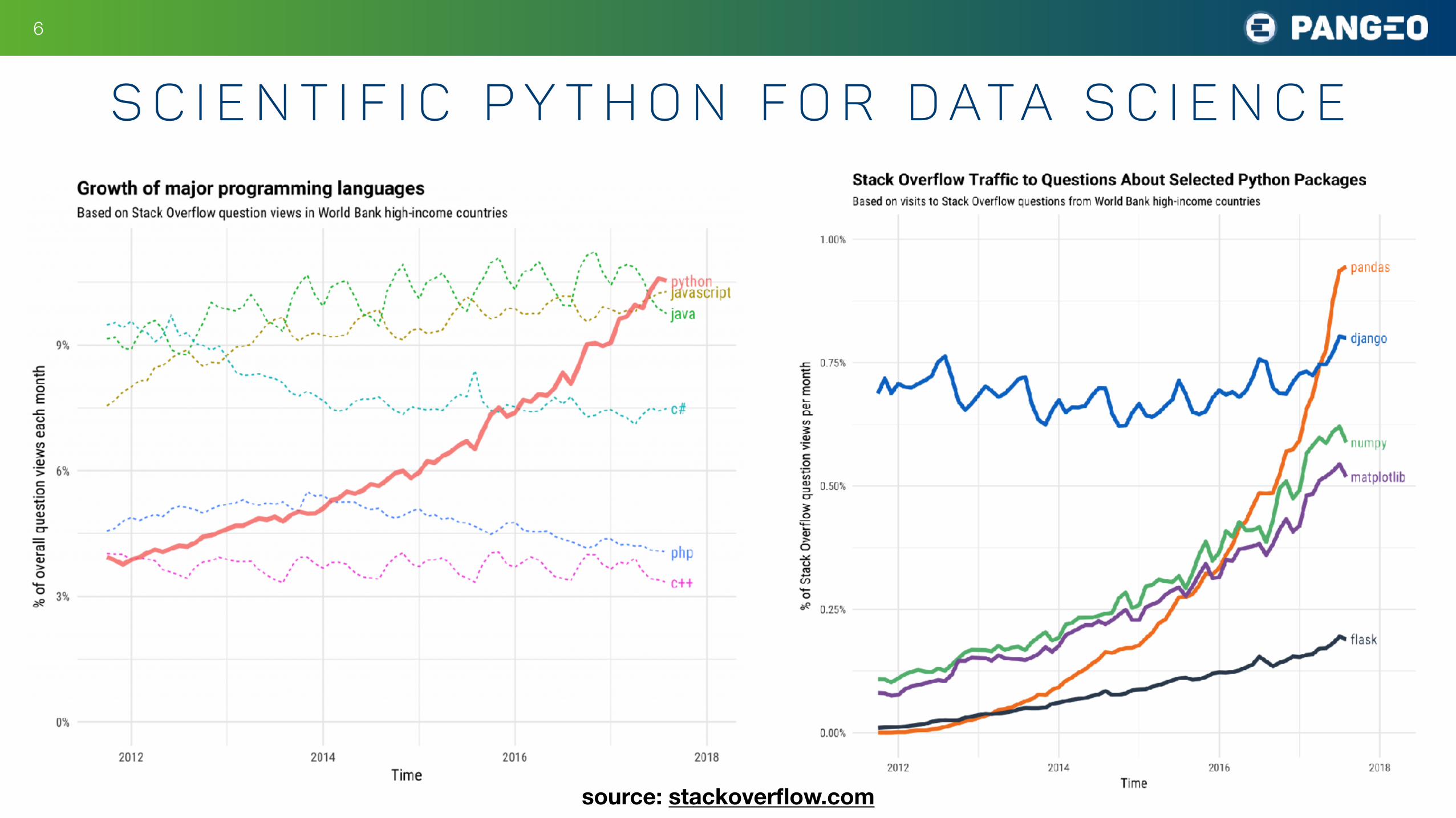
S c i e n t i f i c P y t h o n f o r D ata S c i e n c e

!6

source: stackoverflow.com

aospy

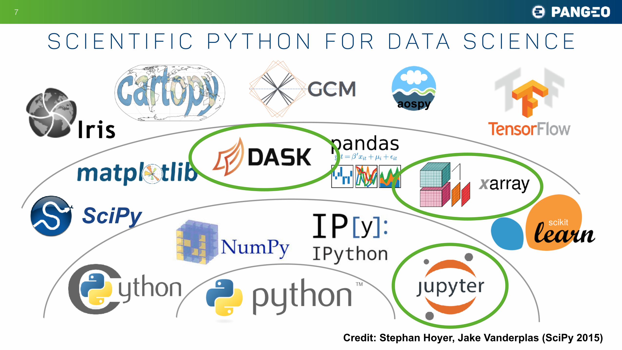
S c i e n t i f i c P y t h o n f o r D ata S c i e n c e

!7

SciPy

Credit: Stephan Hoyer, Jake Vanderplas (SciPy 2015)

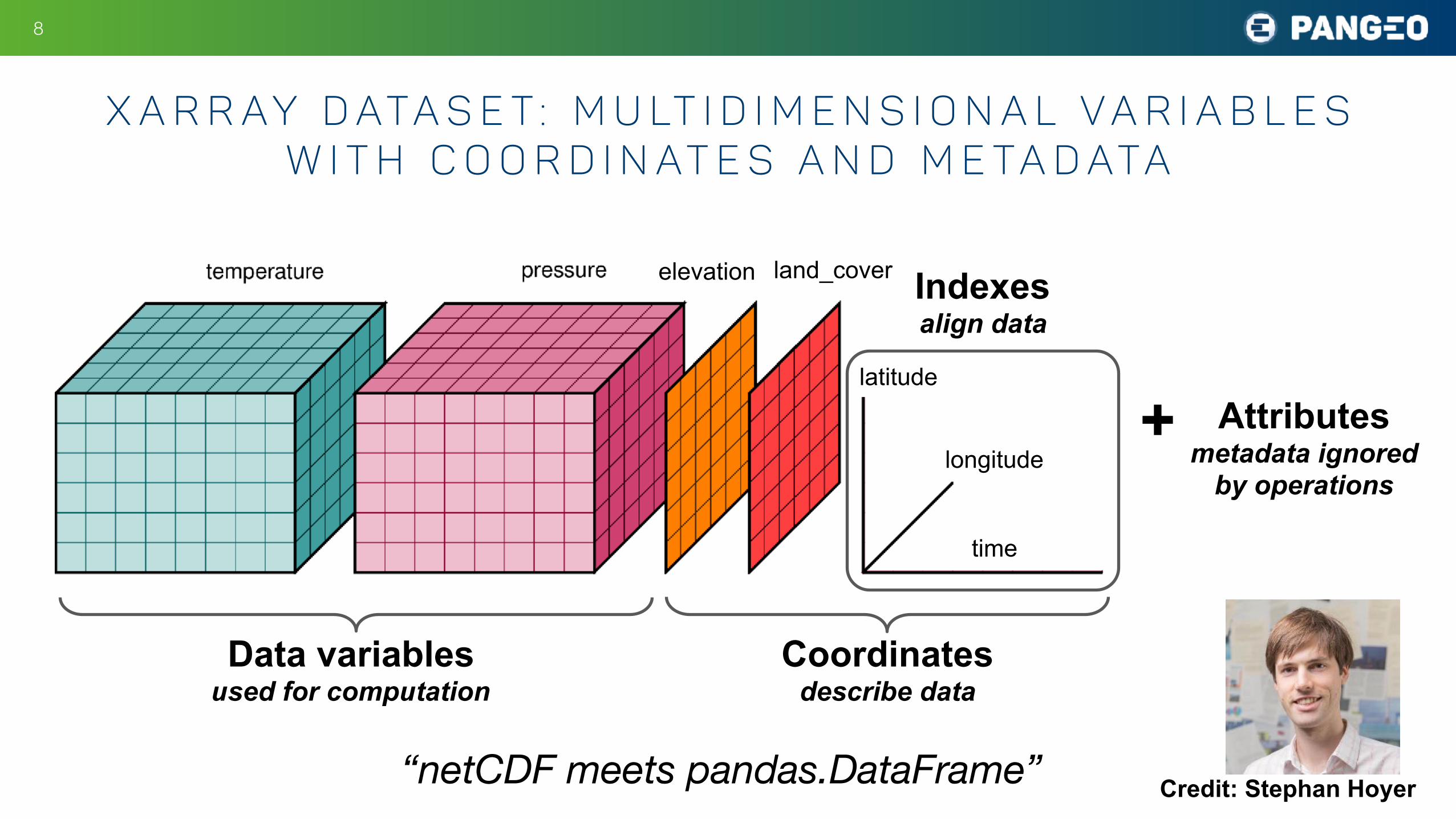
X a r r ay D ata s e t : M u lt i d i m e n s i o n a l V a r i a b l e s w i t h c o o r d i n at e s a n d m e ta d ata

!8

time

longitude

latitude

elevation

Data variables used for computation

Coordinates describe data

Indexes align data

Attributes metadata ignored

by operations

+

land_cover

“netCDF meets pandas.DataFrame” Credit: Stephan Hoyer

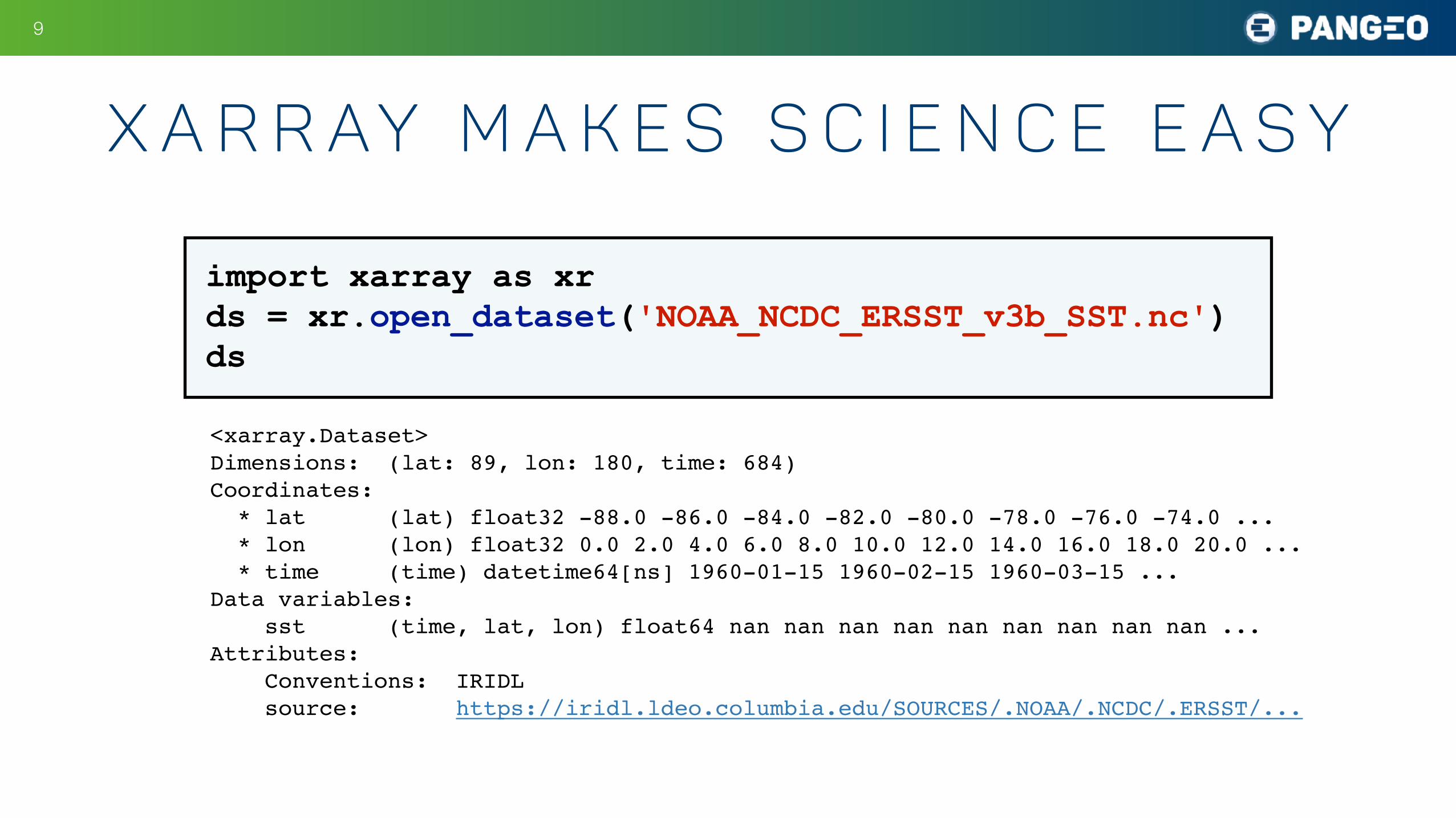
x a r r ay m a k e s s c i e n c e e a s y

!9

import xarray as xr ds = xr.open_dataset('NOAA_NCDC_ERSST_v3b_SST.nc') ds

<xarray.Dataset>Dimensions: (lat: 89, lon: 180, time: 684)Coordinates: * lat (lat) float32 -88.0 -86.0 -84.0 -82.0 -80.0 -78.0 -76.0 -74.0 ... * lon (lon) float32 0.0 2.0 4.0 6.0 8.0 10.0 12.0 14.0 16.0 18.0 20.0 ... * time (time) datetime64[ns] 1960-01-15 1960-02-15 1960-03-15 ...Data variables: sst (time, lat, lon) float64 nan nan nan nan nan nan nan nan nan ...Attributes: Conventions: IRIDL source: https://iridl.ldeo.columbia.edu/SOURCES/.NOAA/.NCDC/.ERSST/...

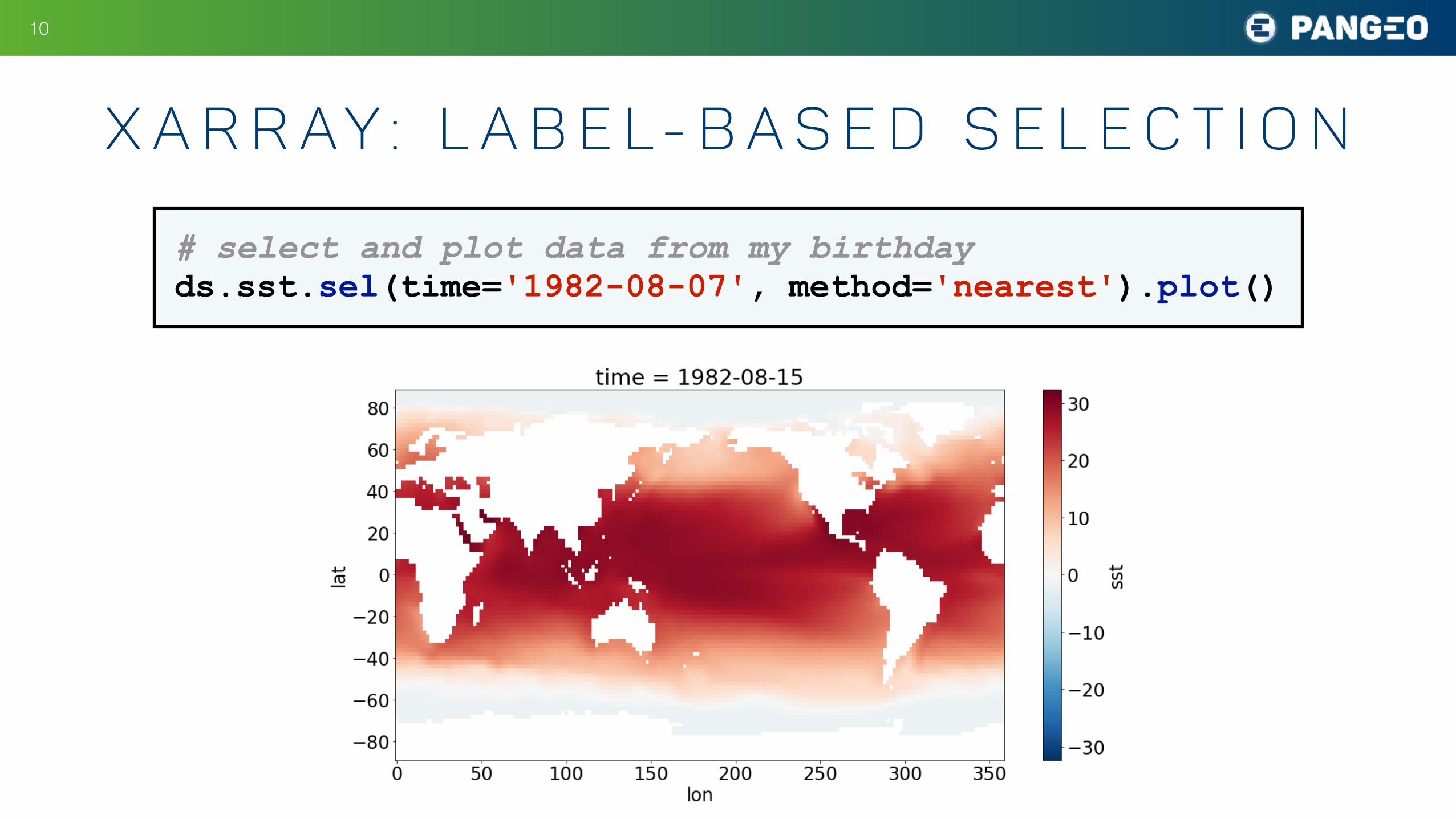
x a r r ay : l a b e l - b a s e d s e l e c t i o n

!10

# select and plot data from my birthday ds.sst.sel(time='1982-08-07', method='nearest').plot()

x a r r ay : l a b e l - b a s e d o p e r at i o n s

!11

# zonal and time mean temperature ds.sst.mean(dim=(‘time', 'lon')).plot()

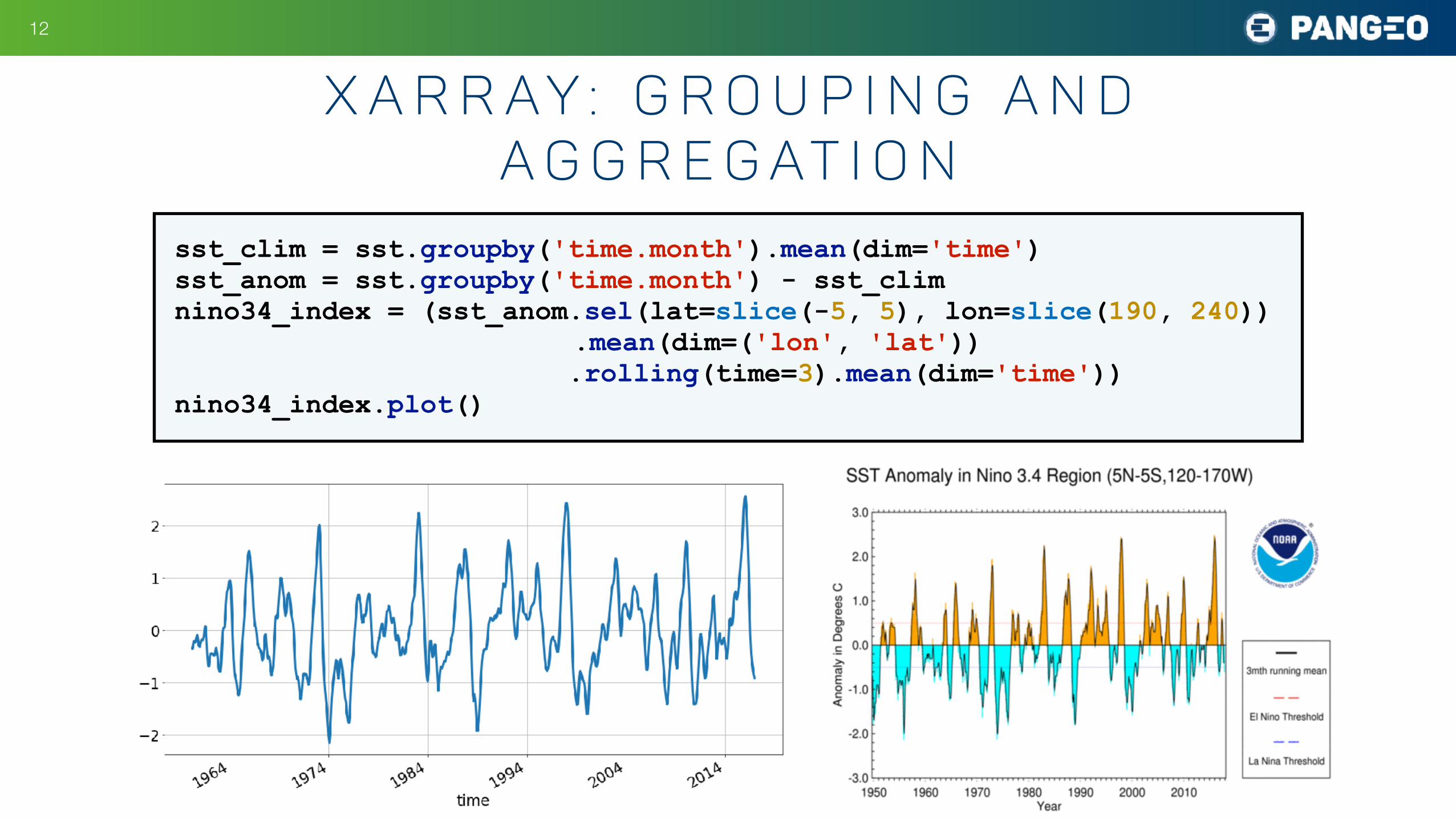
x a r r ay : g r o u p i n g a n d a g g r e g at i o n

!12

sst_clim = sst.groupby('time.month').mean(dim='time') sst_anom = sst.groupby('time.month') - sst_clim nino34_index = (sst_anom.sel(lat=slice(-5, 5), lon=slice(190, 240)) .mean(dim=('lon', 'lat')) .rolling(time=3).mean(dim='time')) nino34_index.plot()

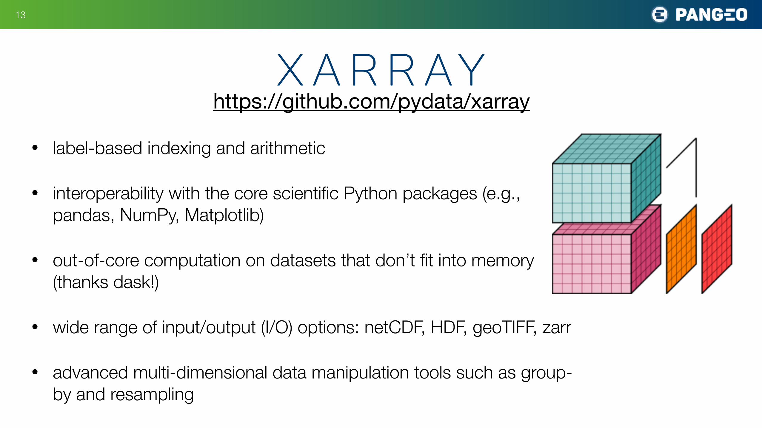
• label-based indexing and arithmetic

• interoperability with the core scientific Python packages (e.g., pandas, NumPy, Matplotlib)

• out-of-core computation on datasets that don’t fit into memory (thanks dask!)

• wide range of input/output (I/O) options: netCDF, HDF, geoTIFF, zarr

• advanced multi-dimensional data manipulation tools such as group-by and resampling

!13

x a r r ayhttps://github.com/pydata/xarray

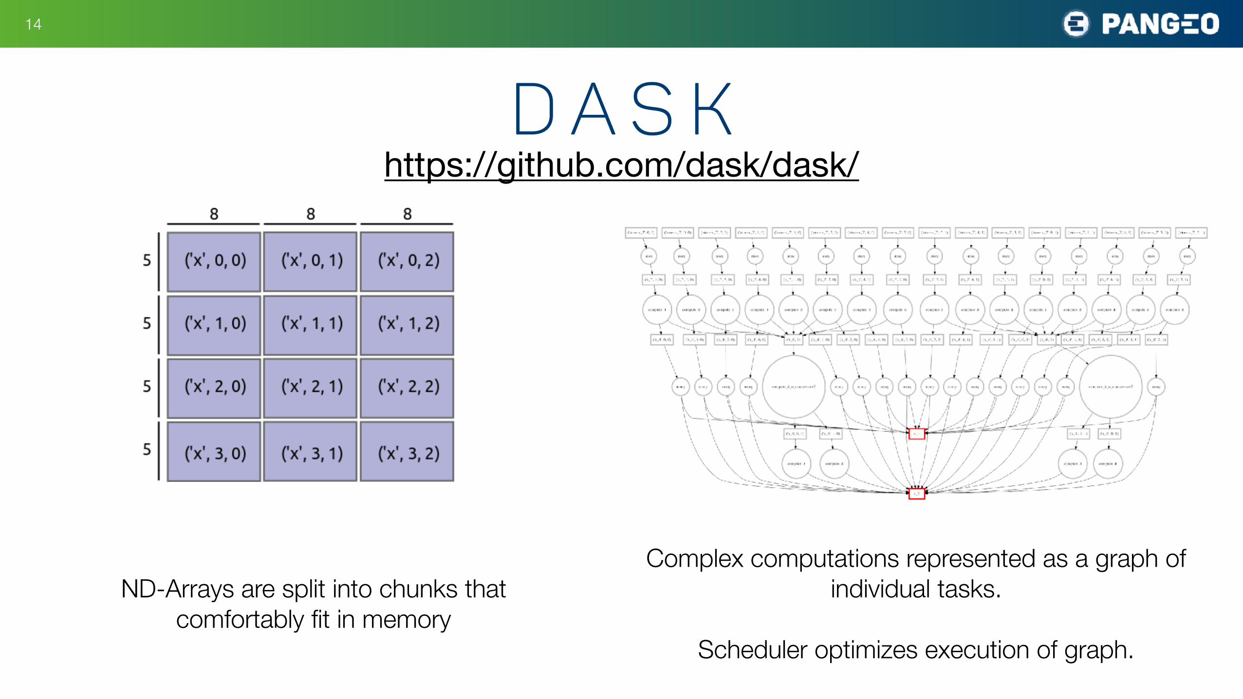
d a s k!14

Complex computations represented as a graph of individual tasks.

Scheduler optimizes execution of graph.

https://github.com/dask/dask/

ND-Arrays are split into chunks that comfortably fit in memory

!15

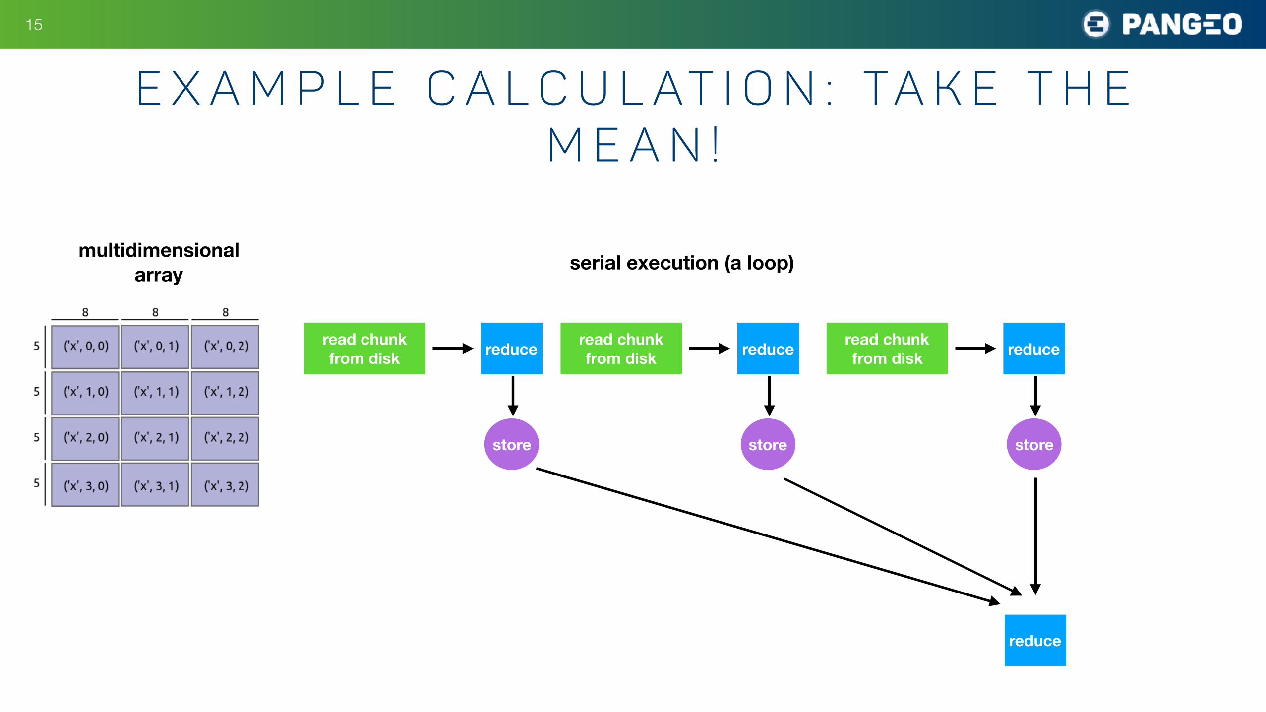
E x a m p l e C a l c u l at i o n : Ta k e t h e M e a n !

multidimensionalarray

read chunk from disk reduce

store

read chunk from disk reduce

store

read chunk from disk reduce

store

serial execution (a loop)

reduce

!16

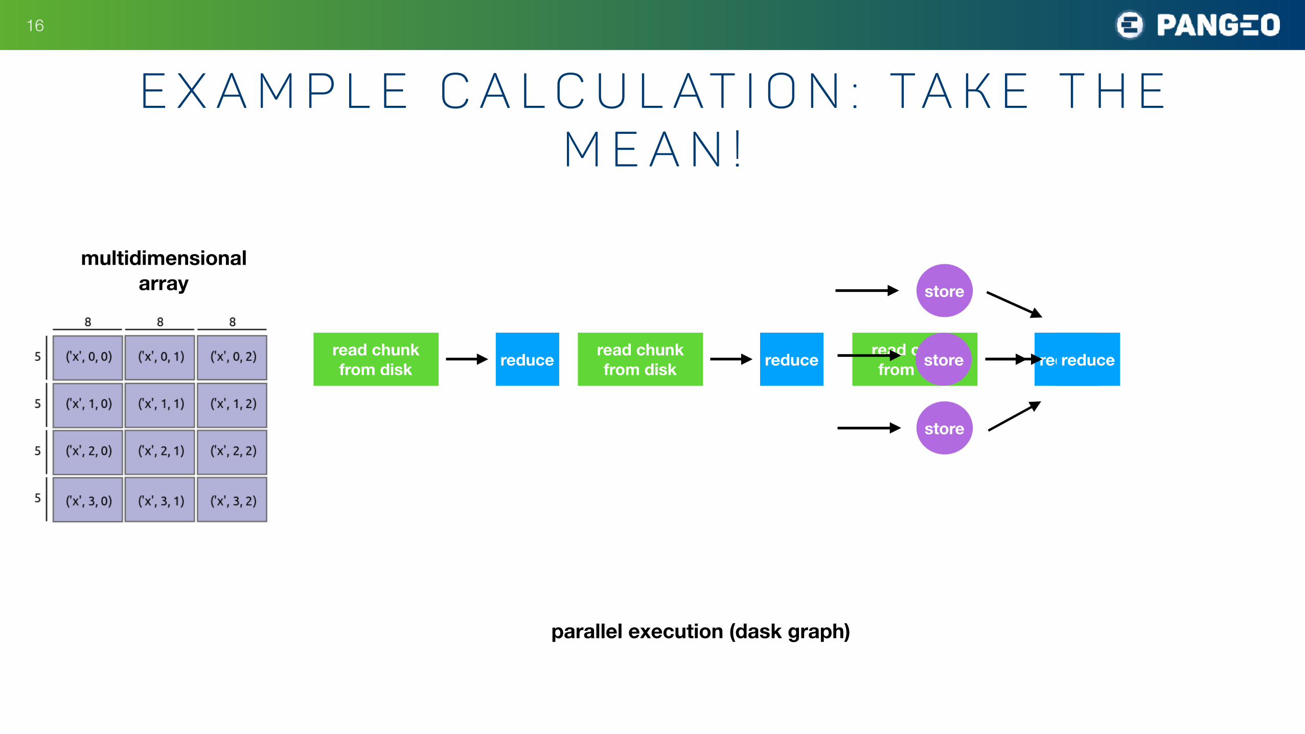
E x a m p l e C a l c u l at i o n : Ta k e t h e M e a n !

multidimensionalarray

read chunk from disk reduce read chunk

from disk reduce read chunk from disk reduce

store

store

store

reduce

parallel execution (dask graph)

• Foster collaboration around the open source scientific python ecosystem for ocean / atmosphere / land / climate science.

• Support the development with domain-specific geoscience packages.

• Improve scalability of these tools to to handle petabyte-scale datasets on HPC and cloud platforms.

!17

P a n g e o P r o j e c t g o a l s

E a r t h c u b e A w a r d T e a m

!18

Ryan Abernathey, Chiara Lepore, Michael Tippet, Naomi Henderson, Richard Seager Kevin Paul, Joe Hamman, Ryan May, Davide Del Vento Matthew Rocklin

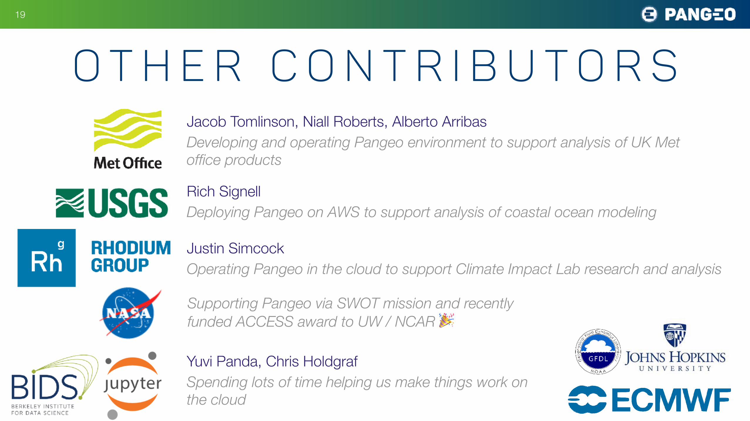
O t h e r C o n t r i b u t o r s!19

Jacob Tomlinson, Niall Roberts, Alberto Arribas Developing and operating Pangeo environment to support analysis of UK Met office products

Rich Signell Deploying Pangeo on AWS to support analysis of coastal ocean modeling

Justin Simcock Operating Pangeo in the cloud to support Climate Impact Lab research and analysis

Supporting Pangeo via SWOT mission and recently funded ACCESS award to UW / NCAR 🎉

Yuvi Panda, Chris Holdgraf Spending lots of time helping us make things work on the cloud

!20

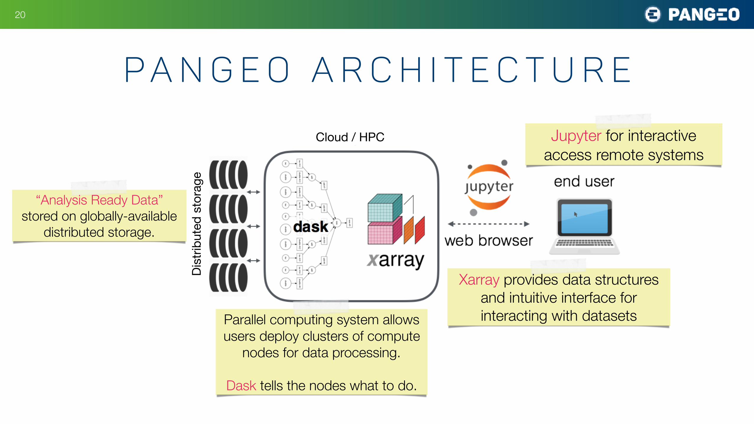
P a n g e o A r c h i t e c t u r e

Jupyter for interactive access remote systems

Cloud / HPC

Xarray provides data structures and intuitive interface for interacting with datasetsParallel computing system allows

users deploy clusters of compute nodes for data processing.

Dask tells the nodes what to do.

Dist

ribut

ed s

tora

ge“Analysis Ready Data”

stored on globally-available distributed storage.

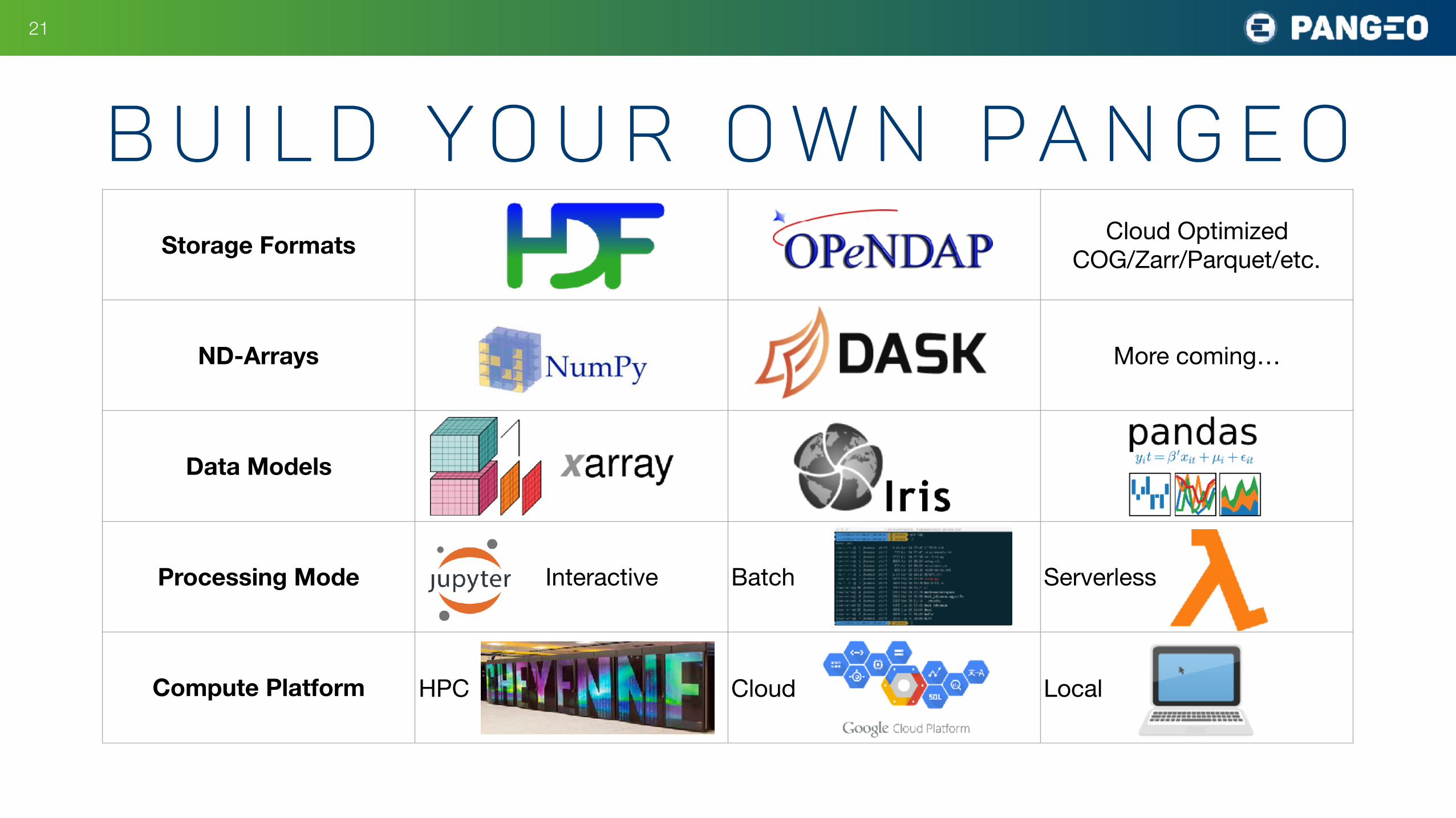
!21

B u i l d y o u r o w n p a n g e oStorage Formats Cloud Optimized

COG/Zarr/Parquet/etc.

ND-Arrays More coming…

Data Models

Processing Mode Interactive Batch Serverless

Compute Platform HPC Cloud Local

!22

P a n g e o D e p l o y m e n t sNASA Pleiades p a n g e o . p y d ata . o r g

NCAR Cheyenne

Over 500 unique users since March!

h t t p : // pa n g e o - data . o r g / d e p l oy m e n t s . h t m l

(Scale using job queue system) (Scale using Kubernetes)

S h a r i n g D ata i n t h e C l o u d

!23

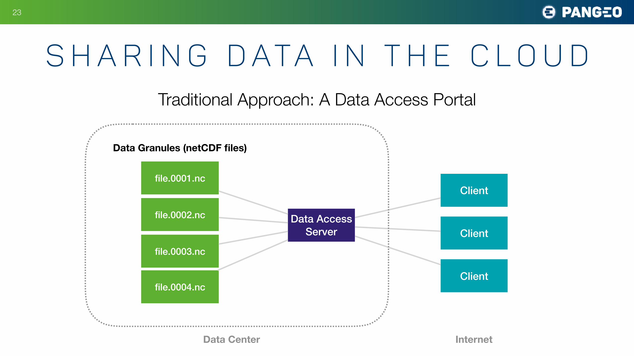
Traditional Approach: A Data Access Portal

Data Access Server

file.0001.nc

file.0002.nc

file.0003.nc

file.0004.nc

Data Granules (netCDF files)

Client

Client

Client

Data Center Internet

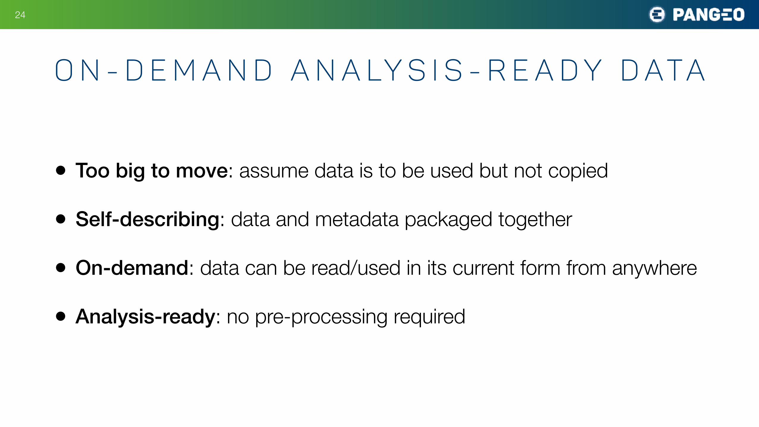
• Too big to move: assume data is to be used but not copied

• Self-describing: data and metadata packaged together

• On-demand: data can be read/used in its current form from anywhere

• Analysis-ready: no pre-processing required

!24

O n - D e m a n d A n a ly s i s - R e a d y D ata

S h a r i n g D ata i n t h e C l o u d

!25

Direct Access to Cloud Object Storage

Catalog

chunk.0.0.0

chunk.0.0.1

chunk.0.0.2

chunk.0.0.3

Data Granules(netCDF files or something new)

Cloud Object Storage

Client

Client

Client

Cloud Data Center

Cloud Compute Instances

!26

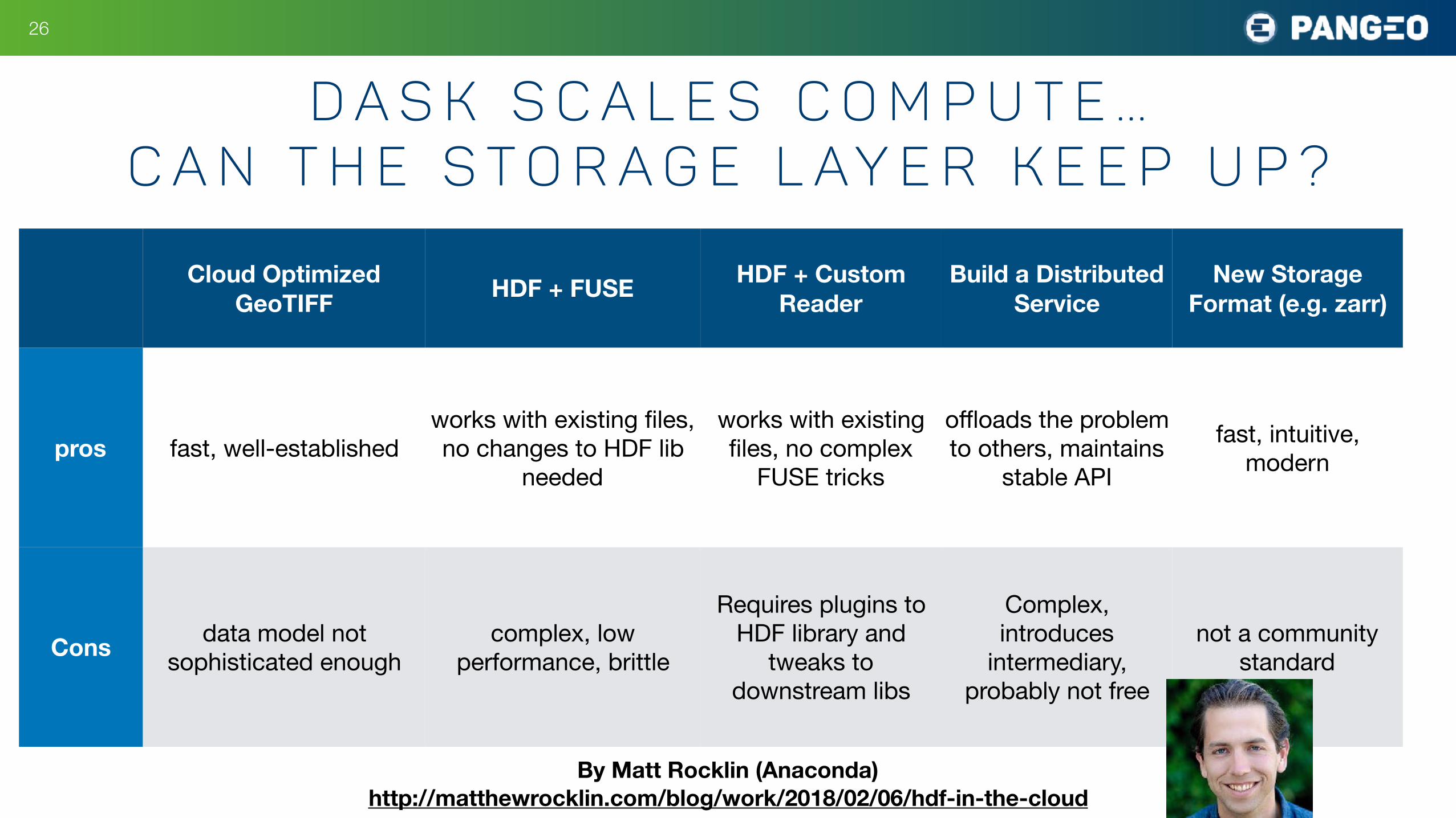
D a s k s c a l e s c o m p u t e … C a n t h e s t o r a g e l ay e r k e e p u p ?

By Matt Rocklin (Anaconda) http://matthewrocklin.com/blog/work/2018/02/06/hdf-in-the-cloud

Cloud Optimized GeoTIFF HDF + FUSE HDF + Custom

ReaderBuild a Distributed

ServiceNew Storage

Format (e.g. zarr)

pros fast, well-establishedworks with existing files, no changes to HDF lib

needed

works with existing files, no complex

FUSE tricks

offloads the problem to others, maintains

stable APIfast, intuitive,

modern

Cons data model not sophisticated enough

complex, low performance, brittle

Requires plugins to HDF library and

tweaks to downstream libs

Complex, introduces

intermediary, probably not free

not a community standard

H o w t o s h a r e a d ata s e t i n t h e c l o u d

!27

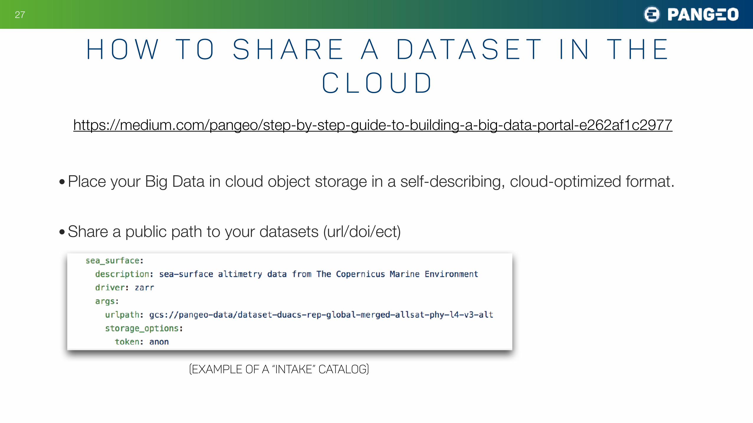
https://medium.com/pangeo/step-by-step-guide-to-building-a-big-data-portal-e262af1c2977

•Place your Big Data in cloud object storage in a self-describing, cloud-optimized format.

•Share a public path to your datasets (url/doi/ect)

(example of a “intake” catalog)

• Access and existing Pangeo deployment on an HPC cluster, or cloud resources (eg. pangeo.pydata.org)

• Adapt Pangeo elements to meet your projects needs (data portals, etc.) and give feedback via github: github.com/pangeo-data/pangeo

• Participate in open-source software development!

!28

H o w t o g e t i n v o lv e dhttp://pangeo-data.org

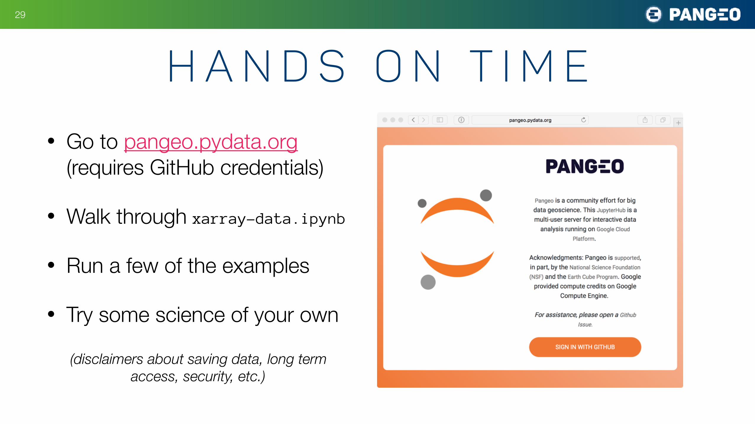
H a n d s o n t i m e!29

• Go to pangeo.pydata.org(requires GitHub credentials)

• Walk through xarray-data.ipynb

• Run a few of the examples

• Try some science of your own

(disclaimers about saving data, long term access, security, etc.)

M o r e o n C l o u d N at i v e G e o s c i e n c e

!30

• Cloud Native Geospatial Part 2: The Cloud Optimized GeoTIFF • Towards On-Demand Analysis Ready Data • https://medium.com/planet-stories

• Step-by-Step Guide to Building a Big Data Portal • https://medium.com/pangeo