Big Data for Engineers – Exercises

Spring 2019 – Week 8 – ETH Zurich

YARN + Spark

Part 1: YARN

What is YARN?Fundamentally, “Yet Another Resource Negotiator”. YARN is a resource scheduler designed to work on existing and new Hadoopclusters.

YARN supports pluggable schedulers. The task of the scheduler is to share the resources of a large cluster among different tenants(applications) while trying to meet application demands (memory, CPU). A user may have several applications active at a time.

Capacity SchedulerThe CapacityScheduler (the default YARN scheduler) gives each USER certain minimum capacity guarantees. With this strategycluster resources are allocated over a set of predetermined queues. Each queue gets only a fraction of the cluster resources. As aresult, each queue has a minimum guaranteed resource allocation.

Consider the hierarchical queues configuration in the figure bellow. Queues are represented by ellipses and the number inside anellipse is the fraction of resource (in %) allocated to the queue. Note that children get absolute memory allocation relative to that oftheir parents.

FIFO SchedulerThe FIFO (First In, First Out) Scheduler is a very simple scheduler that merely places applications in a queue and runs them in theorder they have been submitted. This means that an applications is guaranteed to obtain the resources it has asked for, provided thecluster has them. However, there is no time guarantee.

cluster has them. However, there is no time guarantee.

Fair SchedulerThe Fair Scheduler gives all applications the same priority, distributing resources fairly. It dynamically balances resources between allrunning jobs. This means that as soon as a new job is submitted, the scheduler tries to obtain resources for it such that they areequally distributed again. If preemeption is enabled, it will claim resources more or less instantly, terminating busy containers ifnecessary. Otherwise, it will have to wait until resources free up from another job.

1. ExerciseFor the following exercise, assume a cluster of 100 nodes, each with 10 GB of memory and 2 CPUs allocated for YARN containers.

1.1 – Calculate configured capacities of all leaves of the capacity scheduler above.

SolutionTotal capacity100 nodes x 10 GB = 1000 GB100 nodes x 2 CPUs = 200 CPUs

Spark1000 GB x 0.4 = 400 GB200 CPUs x 0.4 = 80 CPUs

Jack400 GB x 0.3 = 120 GB80 CPUs x 0.3 = 24 CPUs

Phill400 GB x 0.7 = 280 GB80 CPUs x 0.7 = 56 CPUs

MPI1000 GB x 0.1 = 100 GB200 CPUs x 0.1 = 20 CPUs

Jim's lab1000 GB x 0.5 = 500 GB200 CPUs x 0.5 = 100 CPUs

1.2 – Application completion timeline.Recall that free capacity in the cluster can be allocated to applications which have demand for it, regardless of the scheduler beingused (in practice, it is a bit more complicated than this, but you can ignore this for the sake of this exercise). Consider the followingtimelines of events happening in the cluster:

1. In the beginning, the entire cluster is free, with no application in any queues. Jack submits 3 applications with (120 GB, 10 CPUs)resource requirements each. Assume each application takes 1 hour to finish.

2. In the beginning, the entire cluster is free, with no applications in any queues. Jack submits 20 applications with (100 GB, 6CPUs) resource requirements each. After 1 hour, Phill submits 1 application with resource requirements of (50 GB, 10 CPUs).Assume preemption is disabled and each application takes 2 hours to finish.

Explain, for each of the 3 schedulers (ignoring the capacity tree for the other schedulers), how cluster resources would be allocatedacross jobs over time.

SolutionScenario 1.

Capacity Scheduler: All three applications will be launched at the same time regardless of the capacity of the queue, since thereare enough cluster resources to run all three jobs together (120 ∗ 3 ≤ 1000; 10 ∗ 3 ≤ 200).FIFO Scheduler: All three applications will be launched at the same time, since there are enough resources.Fair Scheduler: Again, all three applications will be launched at the same time.

Scenario 2.

Scenario 2.

Capacity Scheduler: 10 applications will be launched at the same time regardless of the capacity of the queue, since there areenough cluster resources to run 10 jobs together (100 ∗ 10 ≤ 1000; 6 ∗ 10 ≤ 200). Since preemption is disabled, Phill will have towait until any resources are freed up before he can claim its minimum capacity. This means Phill's application will start after 2hours, as well as 9 more of Jack's jobs. After 4 hours, the last of Jack's jobs will be launched.FIFO Scheduler: 10 applications will be launched at the same time. After that, since Jack submitted his jobs first, his next 10 willrun, and finally Phill's after 4h.Fair Scheduler: In this case, the outcome is the same as using the capacity scheduler. Note that if Phill had tried to claim morethan its Capacity Scheduler minimum allocation, he would only have been granted it using the Fair Scheduler (since he has theright to half the resources), but not using the Capacity Scheduler (since he's asking for more than he's guaranteed to be given).

Part 2: Spark

1. Setup the Spark cluster on Azure

Create a clusterSign into the azure portal (portal.azure.com).Search for "HDInsight clusters" using the search box at the top.Click on "+ Add".Give the cluster a unique name.In the "Select Cluster Type" choose Spark and a standard Cluster Tier (Finish with pressing "select").In step 2, the container name will be filled in for you automatically. If you want to do the exercise sheet in several sittings, changeit to something you can remember or write it down.Set up a Spark cluster with default configuration. It should cost something around 3.68 sFR/h.Wait for 20 mins so that your cluster is ready.

Important

Remember to delete the cluster once you are done. If you want to stop doing the exercises at any point, delete it and recreate it usingthe same container name as you used the first time, so that the resources are still there.

Access your clusterMake sure you can access your cluster (the NameNode) via SSH:

$ ssh <ssh_user_name>@<cluster_name>-ssh.azurehdinsight.net

If you are using Linux or MacOSX, you can use your standard terminal. If you are using Windows you can use:

Putty SSH Client and PSCP tool (get them at here).This Notebook server terminal (Click on the Jupyter logo and the goto New -> Terminal).Azure Cloud Terminal (see the HBase exercise sheet for details)

The cluster has its own Jupyter server. We will use it. You can access it through the following link:

https://<cluster_name>.azurehdinsight.net/jupyter

You can access cluster's YARN in your browser

https://<cluster_name>.azurehdinsight.net/yarnui/hn/cluster

The Spark UI can be accessed via Azure Portal, see Spark job debugging

You need to upload this notebook to your cluster's Jupyter inorder to execute Python code blocks.To do this, just open the Jupyter through the link given above and use the "Upload" button.

2. Apache Spark ArchitecutureSpark is a cluster computing platform designed to be fast and general purpose. Spark extends the MapReduce model to efficientlycover a wide range of workloads that previously required separate distributed systems, including interactive queries and streamprocessing. Spark offers the ability to run computations in memory.

At a high level, every Spark application consists of a driver program that launches various parallel operations on a cluster. Thedriver program contains your application's main function and defines distributed datasets on the cluster, then applies operations tothem.

Driver programs access Spark through a SparkContext object, which represents a connection to a computing cluster. There is noneed to create a SparkContext; it is created for you automatically when you run the first code cell in the Jupyter

The driver communicates with a potentially large number of distributed workers called executors. The driver runs in its own processand each executor is a separate process. A driver and its executors are together termed a Spark application.

2.1 Understand resilient distributed datasets (RDD)An RDD in Spark is simply an immutable distributed collection of objects. Each RDD is split into multiple partitions, which may becomputed on different nodes of the cluster.

What are RDD operations?

RDDs offer two types of operations: transformations and actions.

Transformations create a new dataset from an existing one. Transformations are lazy, meaning that no transformation isexecuted until you execute an action.Actions compute a result based on an RDD, and either return it to the driver program or save it to an external storage system(e.g., HDFS)

Transformations and actions are different because of the way Spark computes RDDs. Although you can define new RDDs any time,Spark computes them only in a lazy fashion, that is, the first time they are used in an action.

How do I make an RDD?

RDDs can be created from stable storage or by transforming other RDDs. Run the cells below to create RDDs from the sample datafiles available in the storage container associated with your Spark cluster. One such sample data file is available on the cluster at wasb:///example/data/fruits.txt .

In [1]:

fruits = sc.textFile('wasb:///example/data/fruits.txt')yellowThings = sc.textFile('wasb:///example/data/yellowthings.txt')

RDD transformations

Following are examples of some of the common transformations available. For a detailed list, see RDD Transformations

Run some transformations below to understand this better.

In [2]:

# mapfruitsReversed = fruits.map(lambda fruit: fruit[::-1])

In [3]:

# filtershortFruits = fruits.filter(lambda fruit: len(fruit) <= 5)

In [4]:

# flatMapcharacters = fruits.flatMap(lambda fruit: list(fruit))

In [5]:

Starting Spark application

ID YARN Application ID Kind State Spark UI Driver log Current session?

11 application_1557208395088_0015 pyspark3 idle Link Link ✔

SparkSession available as 'spark'.

# unionfruitsAndYellowThings = fruits.union(yellowThings)

In [6]:

# intersectionyellowFruits = fruits.intersection(yellowThings)

In [7]:

# distinctdistinctFruitsAndYellowThings = fruitsAndYellowThings.distinct()

In [8]:

# groupByKeyyellowThingsByFirstLetter = yellowThings.map(lambda thing: (thing[0], thing)).groupByKey()

In [9]:

# reduceByKeynumFruitsByLength = fruits.map(lambda fruit: (len(fruit), 1)).reduceByKey(lambda x, y: x + y)

RDD actions

Following are examples of some of the common actions available. For a detailed list, see RDD Actions.

Run some transformations below to understand this better.

In [10]:

# collectfruitsArray = fruits.collect()yellowThingsArray = yellowThings.collect()print(fruitsArray)print(yellowThingsArray)

In [11]:

# countnumFruits = fruits.count()numFruits

In [12]:

# takefirst3Fruits = fruits.take(3)first3Fruits

In [13]:

# reduceletterSet = fruits.map(lambda fruit: set(fruit)).reduce(lambda x, y: x.union(y))letterSet

Lazy evaluation

Lazy evaluation means that when we call a transformation on an RDD (for instance, calling map() ), the operation is not immediatelyperformed. Instead, Spark internally records metadata to indicate that this operation has been requested. Rather than thinking of anRDD as containing specific data, it is best to think of each RDD as consisting of instructions on how to compute the data that we buildup through transformations. Loading data into an RDD is lazily evaluated in the same way transformations are. So, when we call sc.textFile() , the data is not loaded until it is necessary. As with transformations, the operation (in this case, reading the data)

can occur multiple times.

Finally, as you derive new RDDs from each other using transformations, Spark keeps track of the set of dependencies between

['apple', 'banana', 'canary melon', 'grape', 'lemon', 'orange', 'pineapple', 'strawberry']['banana', 'bee', 'butter', 'canary melon', 'gold', 'lemon', 'pineapple', 'sunflower']

8

['apple', 'banana', 'canary melon']

{'o', 'r', 'a', 'i', 'p', 'g', 'c', ' ', 'l', 'y', 'e', 'w', 'n', 'b', 'm', 't', 's'}

Finally, as you derive new RDDs from each other using transformations, Spark keeps track of the set of dependencies betweendifferent RDDs, called the lineage graph. For instance, the code bellow corresponds to the following graph:

In [14]:

apples = fruits.filter(lambda x: "apple" in x)lemons = yellowThings.filter(lambda x: "lemon" in x)applesAndLemons = apples.union(lemons)print(applesAndLemons.collect())print(applesAndLemons.toDebugString())

Persistence (Caching)

Spark's RDDs are by default recomputed each time you run an action on them. If you would like to reuse an RDD in multiple actions,you can ask Spark to persist it using RDD.persist() . After computing it the first time, Spark will store the RDD contents inmemory (partitioned across the machines in your cluster), and reuse them in future actions. Persisting RDDs on disk instead ofmemory is also possible.

If you attempt to cache too much data to fit in memory, Spark will automatically evict old partitions using a Least Recently Used (LRU)cache policy. For the memory-only storage levels, it will recompute these partitions the next time they are accessed, while for thememory-and-disk ones, it will write them out to disk. In either case, this means that you don't have to worry about your job breaking ifyou ask Spark to cache too much data. However, caching unnecessary data can lead to eviction of useful data and morerecomputation time. Finally, RDDs come with a method called unpersist() that lets you manually remove them from the cache.

Working with Key/Value Pairs

Spark provides special operations on RDDs containing key/value pairs. These RDDs are called pair RDDs. Pair RDDs are a usefulbuilding block in many programs, as they expose operations that allow you to act on each key in parallel or regroup data across thenetwork. For example, pair RDDs have a reduceByKey() method that can aggregate data separately for each key, and a join() method that can merge two RDDs together by grouping elements with the same key. Pair RDDs are also still RDDs.

In [15]:

#Examplerdd = sc.parallelize([("key1", 0) ,("key2", 3),("key1", 8) ,("key3", 3),("key3", 9)])rdd2 = rdd.mapValues(lambda x: (x, 1)).reduceByKey(lambda x, y: (x[0] + y[0], x[1] + y[1]))print(rdd2.collect())print(rdd2.toDebugString())

[u'apple', u'pineapple', u'lemon'](4) UnionRDD[29] at union at NativeMethodAccessorImpl.java:0 [] | PythonRDD[27] at RDD at PythonRDD.scala:52 [] | wasb:///example/data/fruits.txt MapPartitionsRDD[1] at textFile at NativeMethodAccessorImpl.java:0 [] | wasb:///example/data/fruits.txt HadoopRDD[0] at textFile at NativeMethodAccessorImpl.java:0 [] | PythonRDD[28] at RDD at PythonRDD.scala:52 [] | wasb:///example/data/yellowthings.txt MapPartitionsRDD[3] at textFile at NativeMethodAccessorImpl.java:0 [] | wasb:///example/data/yellowthings.txt HadoopRDD[2] at textFile at NativeMethodAccessorImpl.java:0 []

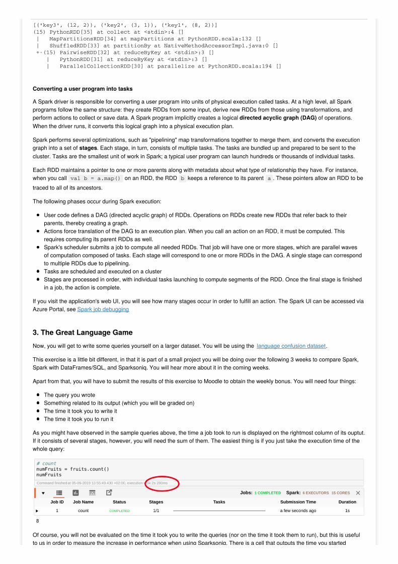
Converting a user program into tasks

A Spark driver is responsible for converting a user program into units of physical execution called tasks. At a high level, all Sparkprograms follow the same structure: they create RDDs from some input, derive new RDDs from those using transformations, andperform actions to collect or save data. A Spark program implicitly creates a logical directed acyclic graph (DAG) of operations.When the driver runs, it converts this logical graph into a physical execution plan.

Spark performs several optimizations, such as "pipelining" map transformations together to merge them, and converts the executiongraph into a set of stages. Each stage, in turn, consists of multiple tasks. The tasks are bundled up and prepared to be sent to thecluster. Tasks are the smallest unit of work in Spark; a typical user program can launch hundreds or thousands of individual tasks.

Each RDD maintains a pointer to one or more parents along with metadata about what type of relationship they have. For instance,when you call val b = a.map() on an RDD, the RDD b keeps a reference to its parent a . These pointers allow an RDD to betraced to all of its ancestors.

The following phases occur during Spark execution:

User code defines a DAG (directed acyclic graph) of RDDs. Operations on RDDs create new RDDs that refer back to theirparents, thereby creating a graph.Actions force translation of the DAG to an execution plan. When you call an action on an RDD, it must be computed. Thisrequires computing its parent RDDs as well.Spark's scheduler submits a job to compute all needed RDDs. That job will have one or more stages, which are parallel wavesof computation composed of tasks. Each stage will correspond to one or more RDDs in the DAG. A single stage can correspondto multiple RDDs due to pipelining.Tasks are scheduled and executed on a clusterStages are processed in order, with individual tasks launching to compute segments of the RDD. Once the final stage is finishedin a job, the action is complete.

If you visit the application's web UI, you will see how many stages occur in order to fulfill an action. The Spark UI can be accessed viaAzure Portal, see Spark job debugging

3. The Great Language GameNow, you will get to write some queries yourself on a larger dataset. You will be using the language confusion dataset.

This exercise is a little bit different, in that it is part of a small project you will be doing over the following 3 weeks to compare Spark,Spark with DataFrames/SQL, and Sparksoniq. You will hear more about it in the coming weeks.

Apart from that, you will have to submit the results of this exercise to Moodle to obtain the weekly bonus. You will need four things:

The query you wroteSomething related to its output (which you will be graded on)The time it took you to write itThe time it took you to run it

As you might have observed in the sample queries above, the time a job took to run is displayed on the rightmost column of its ouptut.If it consists of several stages, however, you will need the sum of them. The easiest thing is if you just take the execution time of thewhole query:

Of course, you will not be evaluated on the time it took you to write the queries (nor on the time it took them to run), but this is usefulto us in order to measure the increase in performance when using Sparksoniq. There is a cell that outputs the time you started

[('key3', (12, 2)), ('key2', (3, 1)), ('key1', (8, 2))](15) PythonRDD[35] at collect at <stdin>:4 [] | MapPartitionsRDD[34] at mapPartitions at PythonRDD.scala:132 [] | ShuffledRDD[33] at partitionBy at NativeMethodAccessorImpl.java:0 [] +-(15) PairwiseRDD[32] at reduceByKey at <stdin>:3 [] | PythonRDD[31] at reduceByKey at <stdin>:3 [] | ParallelCollectionRDD[30] at parallelize at PythonRDD.scala:194 []

to us in order to measure the increase in performance when using Sparksoniq. There is a cell that outputs the time you startedworking before every query. Use this if you find it useful.

For this exercise, you can chose to either set up a local Spark installation on your computer or use an Azure cluster as explainedabove. Both are fine, but a local installation really makes things easier to debug.

If you choose to go for a local installation:

Make sure you have Java 8 or later installed on your computer.Install the latest Spark release. Here are tutorials for Linux, Windows, and MacOS.Launch pyspark with $ pyspark

In any case:

Now either log in to your cluster using SSH as explained above and run the following commands, or of course do it locally:

wget http://data.greatlanguagegame.com.s3.amazonaws.com/confusion-2014-03-02.tbz2

tar -jxvf confusion-2014-03-02.tbz2 -C /tmp

If you're on a cluster:

hdfs dfs -copyFromLocal /tmp/confusion-2014-03-02/confusion-2014-03-02.json /confusion.json

This dowloads the archive file to the cluster, decompresses it and uploads it to HDFS when using a cluster. Now, create an RDD fromthe file containing the entries:

In [16]:

data = sc.textFile('wasb:///confusion.json')

Or locally:

>>> data = sc.textFile('file:///tmp/confusion-2014-03-02/confusion-2014-03-02.json')

Note: from here on, if you're doing things locally, just copy the contents of the cells into the pyspark shell and work on there!

Since some of the queries take a long time to execute, you might want to test them on a smaller subset of the whole dataset. Also,since the entries are JSON records, you will need to parse them and use their respective object representations. You can use thismapping for all queries:

In [17]:

testset = sc.parallelize(data.take(100000))

import jsonentries = data.map(json.loads)test_entries = testset.map(json.loads)

And test it. Is it working?

In [4]:

target_german = test_entries.filter(lambda e: e["target"] == "German").take(1)print(json.dumps(target_german, indent = 4))

Good! Let's get to work. A few last things:

Take into account that some of the queries might have very large outputs, which Jupyter (or sometimes even Spark) won't be

[ { "guess": "German", "target": "German", "country": "AU", "choices": [ "German", "Serbian", "Swedish", "Vietnamese" ], "sample": "e77d97b712adffc39e531e20237a5589", "date": "2013-08-19" }]

Take into account that some of the queries might have very large outputs, which Jupyter (or sometimes even Spark) won't beable to handle. It is normal for the queries to take some time, but if the notebook crashes or stops responding, try restarting thekernel. Avoid printing large outputs. You can print the first few entries to confirm the query has worked, as shown in query 1.Remember to delete the cluster if you want to stop working! You can recreate it using the same container name and yourresources will still be there.Refer to the documentation, as well as the programming guides on actions and transformations linked to above.

And now to the actual queries:

1. Find all games such that the guessed language is correct (=target), and such that this language is Russian.

In [ ]:

from datetime import datetime

# Started working:print(datetime.now().time())

In [4]:

# Query:matching = entries.filter(lambda e: e["target"] == e["guess"] and e["target"] == "Russian").collect()# Only print the first few entriesprint(json.dumps(matching[:3], indent=4))

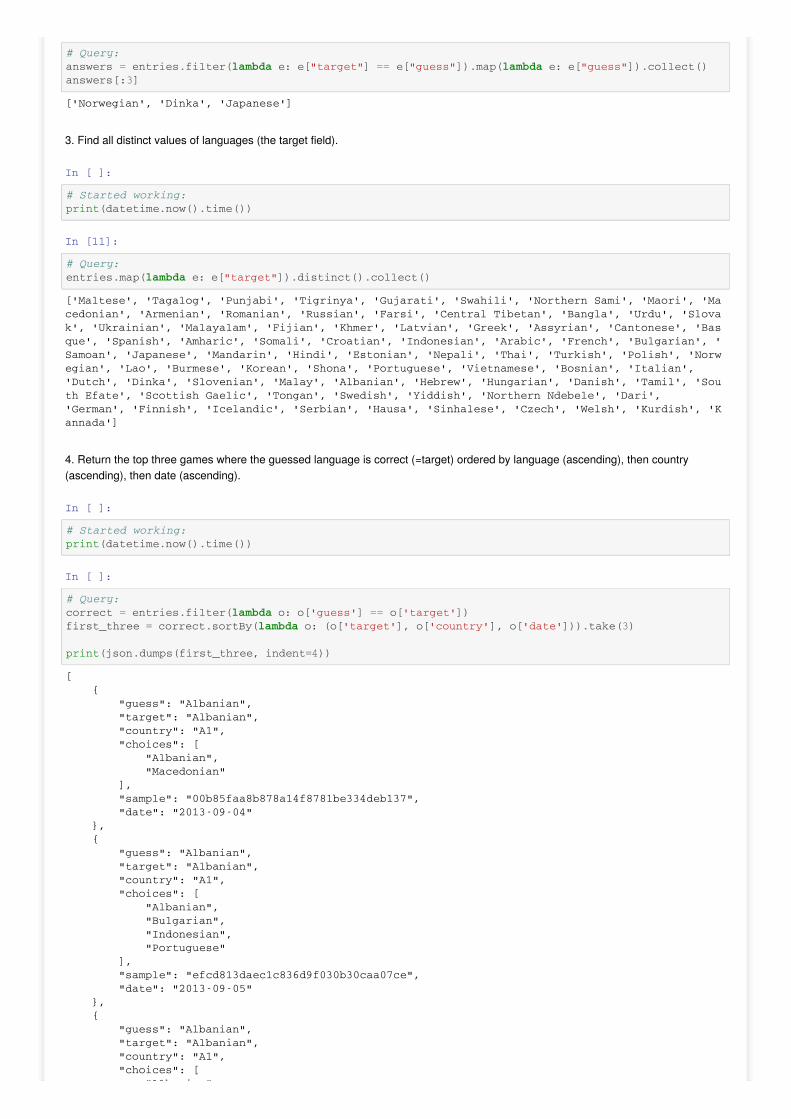
2. List all chosen answers to games where the guessed language is correct (=target).

In [ ]:

# Started working:print(datetime.now().time())

In [4]:

[ { "choices": [ "Lao", "Nepali", "Russian", "Tongan" ], "guess": "Russian", "target": "Russian", "date": "2013-08-19", "country": "AU", "sample": "8a59d48e99e8a1df7e366c4648095e27" }, { "choices": [ "Arabic", "Estonian", "Greek", "Russian" ], "guess": "Russian", "target": "Russian", "date": "2013-08-19", "country": "AU", "sample": "8a59d48e99e8a1df7e366c4648095e27" }, { "choices": [ "Croatian", "Nepali", "Russian", "Slovenian" ], "guess": "Russian", "target": "Russian", "date": "2013-08-20", "country": "AU", "sample": "8a59d48e99e8a1df7e366c4648095e27" }]

In [4]:

# Query:answers = entries.filter(lambda e: e["target"] == e["guess"]).map(lambda e: e["guess"]).collect()answers[:3]

3. Find all distinct values of languages (the target field).

In [ ]:

# Started working:print(datetime.now().time())

In [11]:

# Query:entries.map(lambda e: e["target"]).distinct().collect()

4. Return the top three games where the guessed language is correct (=target) ordered by language (ascending), then country(ascending), then date (ascending).

In [ ]:

# Started working:print(datetime.now().time())

In [ ]:

# Query:correct = entries.filter(lambda o: o['guess'] == o['target'])first_three = correct.sortBy(lambda o: (o['target'], o['country'], o['date'])).take(3)

print(json.dumps(first_three, indent=4))

['Norwegian', 'Dinka', 'Japanese']

['Maltese', 'Tagalog', 'Punjabi', 'Tigrinya', 'Gujarati', 'Swahili', 'Northern Sami', 'Maori', 'Macedonian', 'Armenian', 'Romanian', 'Russian', 'Farsi', 'Central Tibetan', 'Bangla', 'Urdu', 'Slovak', 'Ukrainian', 'Malayalam', 'Fijian', 'Khmer', 'Latvian', 'Greek', 'Assyrian', 'Cantonese', 'Basque', 'Spanish', 'Amharic', 'Somali', 'Croatian', 'Indonesian', 'Arabic', 'French', 'Bulgarian', 'Samoan', 'Japanese', 'Mandarin', 'Hindi', 'Estonian', 'Nepali', 'Thai', 'Turkish', 'Polish', 'Norwegian', 'Lao', 'Burmese', 'Korean', 'Shona', 'Portuguese', 'Vietnamese', 'Bosnian', 'Italian', 'Dutch', 'Dinka', 'Slovenian', 'Malay', 'Albanian', 'Hebrew', 'Hungarian', 'Danish', 'Tamil', 'South Efate', 'Scottish Gaelic', 'Tongan', 'Swedish', 'Yiddish', 'Northern Ndebele', 'Dari', 'German', 'Finnish', 'Icelandic', 'Serbian', 'Hausa', 'Sinhalese', 'Czech', 'Welsh', 'Kurdish', 'Kannada']

[ { "guess": "Albanian", "target": "Albanian", "country": "A1", "choices": [ "Albanian", "Macedonian" ], "sample": "00b85faa8b878a14f8781be334deb137", "date": "2013-09-04" }, { "guess": "Albanian", "target": "Albanian", "country": "A1", "choices": [ "Albanian", "Bulgarian", "Indonesian", "Portuguese" ], "sample": "efcd813daec1c836d9f030b30caa07ce", "date": "2013-09-05" }, { "guess": "Albanian", "target": "Albanian", "country": "A1", "choices": [ "Albanian",

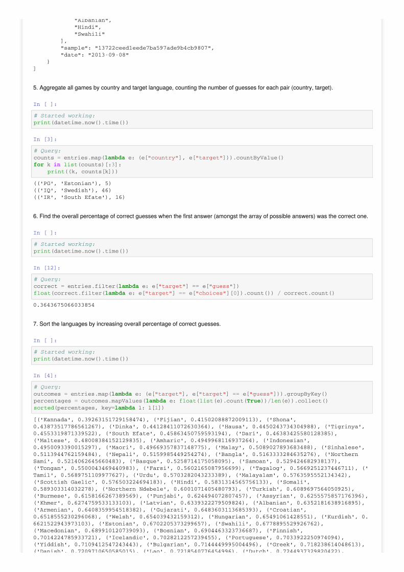
5. Aggregate all games by country and target language, counting the number of guesses for each pair (country, target).

In [ ]:

# Started working:print(datetime.now().time())

In [3]:

# Query:counts = entries.map(lambda e: (e["country"], e["target"])).countByValue()for k in list(counts)[:3]: print((k, counts[k]))

6. Find the overall percentage of correct guesses when the first answer (amongst the array of possible answers) was the correct one.

In [ ]:

# Started working:print(datetime.now().time())

In [12]:

# Query:correct = entries.filter(lambda e: e["target"] == e["guess"])float(correct.filter(lambda e: e["target"] == e["choices"][0]).count()) / correct.count()

7. Sort the languages by increasing overall percentage of correct guesses.

In [ ]:

# Started working:print(datetime.now().time())

In [4]:

# Query:outcomes = entries.map(lambda e: (e["target"], e["target"] == e["guess"])).groupByKey()percentages = outcomes.mapValues(lambda e: float(list(e).count(True))/len(e)).collect()sorted(percentages, key=lambda l: l[1])

"Albanian", "Hindi", "Swahili" ], "sample": "13722ceed1eede7ba597ade9b4cb9807", "date": "2013-09-08" }]

(('PG', 'Estonian'), 5)(('IQ', 'Swedish'), 46)(('IR', 'South Efate'), 16)

0.3643675066033854

[('Kannada', 0.39263151729158474), ('Fijian', 0.41502088872009113), ('Shona', 0.43873517786561267), ('Dinka', 0.44128411072630364), ('Hausa', 0.4450243734304988), ('Tigrinya', 0.4553319871339522), ('South Efate', 0.45863450759593194), ('Dari', 0.46383425580128385), ('Maltese', 0.48008384152129835), ('Amharic', 0.4949968116937264), ('Indonesian', 0.4950093390015297), ('Maori', 0.49669357837148775), ('Malay', 0.5089027893683488), ('Sinhalese', 0.5113944762159484), ('Nepali', 0.5159985449254274), ('Bangla', 0.5163333284635276), ('Northern Sami', 0.5214062645660483), ('Basque', 0.5258714175058095), ('Samoan', 0.529424682938137), ('Tongan', 0.5500043469440983), ('Farsi', 0.5602165087956699), ('Tagalog', 0.5669251237446711), ('Tamil', 0.5689751109977627), ('Urdu', 0.5703282043233389), ('Malayalam', 0.5763595552134342), ('Scottish Gaelic', 0.576503224694183), ('Hindi', 0.5831314565756133), ('Somali', 0.589303314032278), ('Northern Ndebele', 0.6001071405480793), ('Turkish', 0.6089697564050925), ('Burmese', 0.6158166267389569), ('Punjabi', 0.624494072807457), ('Assyrian', 0.6255575857176396), ('Khmer', 0.6274759533133103), ('Latvian', 0.6339322279509824), ('Albanian', 0.6352181638916895), ('Armenian', 0.6408359954518382), ('Gujarati', 0.6483603113685393), ('Croatian', 0.6518555230296068), ('Welsh', 0.654039432159312), ('Hungarian', 0.65491061428551), ('Kurdish', 0.6621522943973103), ('Estonian', 0.6702205373299657), ('Swahili', 0.6778895529926762), ('Macedonian', 0.689910120739093), ('Bosnian', 0.6904463323736687), ('Finnish', 0.7014224785933721), ('Icelandic', 0.7028212257239455), ('Portuguese', 0.7033922250974094), ('Yiddish', 0.7109412547243443), ('Bulgarian', 0.7144449995004496), ('Greek', 0.718238614048613), ('Danish', 0.7209710650585015), ('Lao', 0.7218540776454996), ('Dutch', 0.7244937329820422),

8. Group the games by the index of the correct answer in the choices array and output all counts.

In [ ]:

# Started working:print(datetime.now().time())

In [5]:

# Query:entries.map(lambda e: e["choices"].index(e["target"])).countByValue()

9. What is the language of the sample that has the highest successful guess rate?

In [ ]:

# Started working:print(datetime.now().time())

In [8]:

# Query:outcomes = entries.map(lambda e: (e["target"], e["target"] == e["guess"])).groupByKey()percentages = outcomes.mapValues(lambda e: float(list(e).count(True))/len(e))percentages.top(1, key=lambda e: e[1])

10. Return all games played on the latest day.

In [ ]:

# Started working:print(datetime.now().time())

In [13]:

# Query:latest = entries.groupBy(lambda e: e["date"]).top(1)[0]games = list(latest[1])

print(json.dumps(games[:3], indent=4))

('Danish', 0.7209710650585015), ('Lao', 0.7218540776454996), ('Dutch', 0.7244937329820422), ('Slovenian', 0.7330842673308426), ('Serbian', 0.7334560654783964), ('Central Tibetan', 0.7345248068509728), ('Norwegian', 0.7624699116246504), ('Swedish', 0.7643676218036267), ('Romanian', 0.7649735701351673), ('Hebrew', 0.7747572815533981), ('Polish', 0.7802123726064699), ('Slovak', 0.7806107364597559), ('Czech', 0.7871233970498145), ('Ukrainian', 0.8139437321377068), ('Thai', 0.8152080400437979), ('Arabic', 0.8297439701255851), ('Cantonese', 0.8317228973279747), ('Vietnamese', 0.8415435010399721), ('Mandarin', 0.8595242653097771), ('Japanese', 0.8603833797583054), ('Korean', 0.8681718372403979), ('Russian', 0.877602013410667), ('Italian', 0.8921389559328466), ('Spanish', 0.8956432115670598), ('German', 0.9197634593055483), ('French', 0.9382414927447232)]

defaultdict(<class 'int'>, {0: 5870142, 1: 6008820, 2: 2822396, 3: 1164825, 4: 424676, 5: 143174, 6: 47835, 7: 17058, 8: 6863, 9: 3463, 10: 1972})

[('French', 0.9382414927447232)]

[ { "choices": [ "Danish", "Swedish" ], "guess": "Swedish", "target": "Swedish", "date": "2014-03-01", "country": "DE", "sample": "6640b78667f0ab23077e4a0b51568f89" }, { "choices": [ "Latvian", "Swahili" ], "guess": "Latvian", "target": "Swahili",

4. Exercise1. Why is Spark faster than Hadoop MapReduce?2. Study the queries you wrote using Spark UI. Observe how many stages they have.3. Which of the graphs below are DAGs?

Solution1. There are many reasons for that. Firstly, Spark processes data in-memory while Hadoop MapReduce persists back to the disk

after a map or reduce action. Secondly, Spark pipelines transformations to merge them into stages.2. Follow the following instructions3. DAGs: 2,3,4,5,7

5. True or FalseSay if the following statements are true or false, and explain why.

1. Each RDD is split into multiple partitions, which may be computed on different nodes of the cluster.2. Transformations construct a new RDD from a previous one and immediately calculate the result3. Spark's RDDs are by default recomputed each time you run an action on them4. After computing an RDD, Spark will store its contents in memory and reuse them in future actions.

"date": "2014-03-01", "country": "GB", "sample": "1b959fe55794f6d4e1ea038bfe336759" }, { "choices": [ "Croatian", "Gujarati" ], "guess": "Gujarati", "target": "Croatian", "date": "2014-03-01", "country": "US", "sample": "849aa9c6c726b2ea26c84eec857817f0" }]

4. After computing an RDD, Spark will store its contents in memory and reuse them in future actions.5. When you derive new RDDs using transformations, Spark keeps track of the set of dependencies between different RDDs.

Solution1. True2. False. Spark will not begin to execute until it sees an action.3. True4. False. Users have to use persist() or cache() for that.5. True