bifurcation analysis, chaos and control in the burgers mapping

ISSN 1749-3889 (print), 1749-3897 (online)International Journal of Nonlinear Science

Vol.4(2007) No.3,pp.171-185

Bifurcation Analysis, Chaos and Control in the Burgers Mapping

E. M. ELabbasy, H. N. Agiza, H. EL-Metwally, A. A. Elsadany ∗

Department of Mathematics, Faculty of Science, Mansoura UniversityMansoura 35516, Egypt

(Received 18 April 2007, accepted 29 June 2007)

Abstract: In this paper, the bifurcation analysis for Burgers mapping has been studied. Theexistence and stability of the fixed points of this map was derived. The conditions of existencefor pitchfork bifurcation, flip bifurcation and Neimark-Sacker bifurcation are derived by usingcenter manifold theorem and bifurcation theory. The control of the map around stable Neimark-Sacker bifurcation has been achieved by using feedback polynomial controller technique. Thecomplex dynamics, bifurcations and chaos are displayed by numerical simulations.

Key words: Burgers mapping; Neimark-Sacker bifurcation; Chaotic behavior; feedback con-troller of polynomial functions

1 Introduction

The Burgers mapping is a discretisation of a pair of coupled differential equations which were used byBurgers [1] to illustrate the relevance of the concept of bifurcation to the study of hydrodynamics flows.These equations are indeed a sort of Lorenz model; being in two dimensions they cannot exhibit complextrajectories (see [2]). The Burgers mapping is defined in the following way [2,3]:

{xn+1 = (1− ν)xn − y2

n,yn+1 = (1 + µ)yn + xnyn.

(1)

In [3], the map (1) has been discussed by using the numerical methods. They proved numerically, thatBurgers mapping are produced a much richer set of dynamic patterns than those observed in continuouscase [3,2]. Nevertheless, they have not given theoretical analysis. In this paper we deduce theoreticalanalysis for bifurcations phenomenon and the polynomial type controller [4] to achieve control of chaoticattractor around stable Neimark-Sacker bifurcation for map (1). Jing group have been applied the forwardEuler scheme for the BVP oscillator, FitzHugh-Nagumo system and Predator-prey [5,6,7], they investigatedthe dynamical behaviors in detail as discrete dynamical systems by using the qualitative analysis and centermanifold theorem. In addition, Bifurcations and chaos of the delayed ecological model has been examinedin [8]. Recently, Zhang et al. applied the forward Euler scheme for the simple predator-prey model [9], andthey studied the dynamical behaviors by using the qualitative analysis and center manifold theorem.

This paper is organized as follows. In section 2, the existence and stability of the fixed points andthe qualitative behavior and bifurcations of the map (1) are examined by using the qualitative theory andbifurcation theory. Also, the conditions of existence for pitchfork bifurcation, flip bifurcation and Neimark-Sacker bifurcation deduced and proved. In section 3, we applied the controller technique of Chen-Yu [4] forcontrol this map around stable Neimark-Sacker bifurcation. In section 4, the complex behaviors for the mapvia computing bifurcation diagrams, strange attractors and Lyapunov exponents by numerical simulationswere demonstrated. Finally, section 5 draws the conclusion.

∗Corresponding author. E-mail address: [email protected]

Copyright c©World Academic Press, World Academic UnionIJNS.2007.12.15/109

172 International Journal of Nonlinear Science,Vol.4(2007),No.3,pp. 171-185

2 Existence and stability of fixed points and bifurcations

In this section, we first determine the existence of the fixed points of the map (1), then investigate theirstability by calculating the eigenvalues for the Jacobian matrix of the map (1) at each fixed point, andsufficient conditions of existence for pitchfork bifurcation flip bifurcation and Neimark-Sacker bifurcationby using qualitative theory and bifurcation theory.

By simple computation, the map (1) has the following three fixed points:(i) E0(0, 0) is trivial fixed point,(ii) E1(−µ,

√µν) is interior fixed point exist for µν > 0, and

(iii) E2(−µ,−√µν) is the other interior fixed point. Where E1 and E2 are symmetric fixed points ofcoordinates.

Next we will investigate qualitative behaviors of the map (1). The local dynamics of map (1) in aneighborhood of a fixed point is dependent on the Jacobian matrix of (1). The Jacobian matrix of map (1) atthe state variable is given by

J(x, y) =(

1− ν −2yy 1 + µ + x

). (2)

2.1 Bifurcations of E0(0, 0)

We consider the Jacobian matrix at E0 which has the form

J(E0) =(

1− ν 00 1 + µ

), (3)

which has two eigenvalues λ1 = 1− ν and λ2 = 1 + µ. From the above one can make conclusions:

Proposition 1 (1) When 0 < ν < 2 and −2 < µ < 0, E0 is a stable node (sink); (2) When ν > 2and µ > 0, E0 is unstable node (source); (3) When ν > 2 and −2 < µ < 0,or when 0 < ν < 2 andµ > 0, E0 is saddle point; (4) When ν = 0 or 2 and |λ2| 6= 1 or µ = −2 or µ = 0 and |λ1| 6= 1, E0 is anon-hyperbolic fixed point.

Considering that µ is a bifurcation parameter, and E0 is a non-hyperbolic fixed point for µ = 0 orµ = −2, so the stability and bifurcations will be discussed in the following part.

If µ = 0, then J(E0) has two eigenvalues λ1 = 1− ν and λ2 = 1. The fact that the fixed point E0 is apitchfork bifurcation point requires the following proposition.

Proposition 2 If µ = 0 and ν 6= 0, the map (1) undergoes a pitchfork bifurcation at E0. Moreover the maphas only one fixed point.

Proof. Let σn = µ, such that parameter σn be a new dependent variable, the map (1) can be rewritten in thefollowing form:

xn+1

σn+1

yn+1

=

1− ν 0 00 1 00 0 1

xn

σn

yn

+

−y2n

0xnyn + σnyn

.

By the center manifold theory there exists a center manifold of the map (1), which can expressed locally asfollows:

W c(E0) = {(x, y, σ) ∈ R3 |y = w(x, σ), w(0, 0) = Dw(0, 0) = 0, |x| < ε, |y| < δ},

Assume that w(y, σ) has the following form

xn = w(yn, σn) = a1y2n + a2ynσn + a3σ

2n + o((|xn|+ |yn|)3),

which must satisfyw(y + ynw + ynσn, σn+1) = (1− ν)w − y2

n.

IJNS email for contribution: [email protected]

E. M. ELabbasy, H. N. Agiza, H. EL-Metwally, A. A. Elsadany: Bifurcation Analysis, Chaos and· · · 173

Thus, we can obtain that

a1 = −1ν

and a2 = a3 = 0,

therefore, we have xn = w(yn, σn) = −1ν

x2n, and the map is restricted to the center manifold, which given

by

f1 : yn+1 = yn + σnyn − 1ν

y3n − o((|yn|+ |σn|)4).

Since∂2f1

∂yn∂σn

∣∣(0,0) = 1 6= 0,

∂3f1

∂y3n

∣∣(0,0) = −6

ν6= 0 and f̃1(y, σ) = y + σy − 1

νy3 is odd function for y,

then map (1) undergoes a pitchfork bifurcation at E0. If ν > 0 , then the map (1) undergoes a supercriticalpitchfork bifurcation, whereas the map (1) undergoes a subcritical pitchfork bifurcation when ν < 0.Thiscompletes the proof

Now the flip bifurcation of the map (1) at E0 is considered. If µ = −2, then J(E0) has two eigenvaluesλ1 = 1−ν and λ2 = −1. The fact that the fixed point E0 is a flip bifurcation point is given by the followingproposition.

Proposition 3 If µ = −2, ν 6= 0, the map (1) undergoes a flip bifurcation at E0.

Let σn = µ+2, such that parameter σn be a new dependent variable, the map (1) can be rewritten in thefollowing form:

xn+1

σn+1

yn+1

=

1− ν 0 00 −1 00 0 −1

xn

σn

yn

+

−y2n

0xnyn + σnyn

.

Assume that w(y, σ) has the following form:

xn = w(yn, σn) = b1y2n + b2ynσn + b3σ

2n + o((|yn|+ |σn|)3).

It must satisfy

w(−yn + ynw + σnyn, σn+1) = (1− ν)w − y2n.

Thus, we can obtain that

b1 = −1ν

and b2 = b3 = 0,

therefore, we have xn = w(yn, σn) = −1ν

y2n, and the map is restricted to the center manifold, which given

by

f2 : yn+1 = −yn + σnyn − 1ν

y3n − o((|σn|+ |yn|)4).

Since

α1 = (∂f2

∂σn

∂2f2

∂y2n

+ 2∂2f2

∂yn∂σn)∣∣(0,0) = 2 6= 0,

α2 = (12(∂2f2

∂y2n

)2 +13

∂3f2

∂y3n

)∣∣(0,0) = −2

ν< 0,

then map (6.1) undergoes a flip bifurcation at E0. If ν > 0 , then the map (1) undergoes a supercritical flipbifurcation, whereas the map (1) undergoes a subcritical bifurcation when ν < 0. This complete the proof

IJNS homepage:http://www.nonlinearscience.org.uk/


2.2 Bifurcation of fixed point E1(−µ,√

µν)

We consider the Jacobian matrix at E1 which has the form

J(E1) =(

1− ν −2√

νµ√νµ 1

), (4)

which has two eigenvalues λ1,2 = 12(2 − ν ±

√(2− ν)2 − 4(1− ν + νµ)). E1(−µ,

√µν) is nontrivial

fixed point. Under certain conditions, it can be obtained that map (1) also undergoes pitchfork bifurcationand flip bifurcation at E1(−µ,

√µν). This will be shown by the following two propositions.

Proposition 4 If ν2 − 4µν > 0 and µ = 0, the map (1) undergoes a pitchfork bifurcation at E1. Moreoverthe map has only one fixed point.

Proof. The proof is similar to the proof of proposition 2.

Proposition 5 If ν2 − 4µν > 0 and µ =ν − 2

ν, ν 6= 2 the map (1) undergoes a flip bifurcation at E1.

Proof. In order to prove this result, we consider the eigenvalues of Jacobian matrix at E1 which has theform

J(E1) =(

1− ν −2√

νµ√νµ 1

),

which has two eigenvalues are λ1,2 = 12(2 − ν ±

√(2− ν)2 − 4(1− ν + νµ)). For µ = ν−2

ν , the twoeigenvalues becomes λ1 = 3− ν and λ2 = −1.

Let ζn = xn + ν, ηn = yn −√νµ, σn =√

µ−√

ν−2ν and σn be a new dependent parameters, the map

(1) becomes

ζn+1

σn+1

ηn+1

=

1− a 0 −2√

ν − 20 −1 0√

ν − 2 0 1

+

2√

νσnηn − η2n

0√νσnζn + ζnηn

. (5)

Let

T =

−√ν − 2 0 10 1 0

1 0 −√

ν − 22

.

By the following transformation

ζn

σn

ηn

= T

un

δn

ϑn

the map (5) becomes

un+1

δn+1

ϑn+1

=

(3− ν) 0 00 −1 00 0 −1

un

δn

ϑn

+

ψ(un, δn, ϑn)0

φ(un, δn, ϑn)

, (6)

where

ψ(un, δn, ϑn) =4√

ν√

ν − 2ν − 4

δnun − ν√

ν

ν − 4δnϑn +

3√

ν − 2ν − 4

u2n −

2(ν − 1)ν − 4

unϑn +(ν − 2)

√ν − 2

ν − 4ϑ2

n

φ(un, δn, ϑn) =2ν√

ν

ν − 4δnun − 4

√ν√

ν − 2ν − 4

δnϑn +2(ν − 1)ν − 4

u2n −

(ν + 2)√

ν − 2ν − 4

unϑn +3(ν − 2)2(ν − 4)

ϑ2n

Considerun = w(ϑn, δn) = c1ϑ

2n + c2ϑnδn + c3δ

2n + o((|ϑn|+ |δn|)3),



which must satisfy that

w(−ϑn + φ(w(ϑn, δn), δn, ϑn)) = (3− ν)w(ϑn, δn) + φ(w(ϑn, δn), δn, ϑn),

Thus we can obtain that

c1 =√

ν − 2ν − 4

, c2 = − ν√

ν

(ν − 2)(ν − 4)and c3 = 0

and the map is restricted to the center manifold, which is given by

f3 : ϑn+1 = −ϑn − 4√

ν√

ν − 2ν − 4

ϑnδn +32

(ν − 2)(ν − 4)

ϑ2n +

ν(2ν − 4 + (ν + 2)√

ν)(ν − 4)2

√ν − 2

ϑ2nδn

− 2ν3

(ν − 2)(ν − 4)2ϑnδ2

n −(ν2 − 4)(ν − 4)2

ϑ3n + o((|ϑn|+ |δn|)4)

Since

α1 = (∂f3

∂δn

∂2f3

∂ϑ2n

+ 2∂2f3

∂ϑn∂δn)∣∣(0,0) = −8

√ν√

ν − 2ν − 4

6= 0 for ν 6= 2, 4

α2 = (12(∂2f3

∂ϑ2n

)2 +13

∂3f3

∂ϑ3n

)∣∣(0,0) =

ν2 − 36ν + 684(ν − 4)2

6= 0 for ν 6= 2, 4

It is clear that α2 > 0 when ν < 2 and α2 < 0 when ν > 2. Then fixed point E1 is a subcritical flipbifurcation point of map (1) when ν < 2, whereas the map (1) undergoes a supercritical bifurcation ifν > 2. This completes the proof.

Next, the Neimark-Sacker bifurcation at E1 will be discussed.

2.2.1 Neimark-Sacker bifurcation

Consider the following two-dimensional map:

Xn+1 = F (Xn, α) (7)

where Xn = (xn, yn) and Fα = (f(xn, yn, α), g(xn, yn, α)) be a one-parameter family of map of R2.The map (7) exhibits Neimark-Sacker bifurcation ( discrete Hopf bifurcation ) if a simple pair of complexconjugate eigenvalues of the linearized map crosses the unit circle [4,10].

In order to study the Neimark-Sacker bifurcation of the interior fixed point of studied map, the followingTheorem must be consider firstly.

Theorem 6 (Neimark-Sacker bifurcation [11-13]). Let Fα be a one parameter family of map of R2 satisfy-ing :

(i) Fα(0) = 0 for α near 0;(ii) DFα(0) has two complex eigenvalues λ(α), λ(α) for α near 0 with |λ(0)| = 1;(iii)d|λ(α)|

dα |α=0 > 0;(iv) λ = λ(0) is not an m-th root of unity for m = 1, 2, 3, 4.

Then there is a smooth α−dependent change of coordinates bring Fα into the form

Fα(X) = Gα(U) + O(|U |5) for U ∈ R2

where U = (u, v) and G = (g1, g2).

Moreover, for all sufficiently small positive (negative) α, Fα has an attracting (repelling) invariant circleif l(0) < 0 (l(0) > 0) respectively; and l(0) is given by the following formula:

l(0) = −Re[(1− 2λ)λ2

(1− λ)γ20γ11]− 1

2|γ11|2 − |γ02|2 + Re(λγ21). (8)



where

γ20 =18[(g1uu − g1vv + 2g2uv) + i(g2uu − g2vv − 2g1uv)],

γ11 =14[(g1uu + g1vv) + i(g2uu + g2vv)],

γ02 =18[(g1uu − g1vv − 2g2uv) + i(g2uu − g2vv + 2g1uv)],

γ21 =116

[(g1uuu + g1uvv + g2uuv + g2vvv) + i(g2uuu + g2uvv − g1uuv − g1vvv)].

The calculation of l(0) is given by Wan [12].

2.2.2 Neimark-Sacker bifurcation of fixed point E1(−µ,√

µν)

In this subsection we discuss the Neimark-Sacker bifurcation for fixed point E1(−µ,√

µν) by using abovetheorem. The Jacobian matrix of the map (1) at the fixed point E1 is

J(E1) =(

1− ν −2√

µν√µν 1

). (9)

The characteristic equation of the map (1) at the point E1 is

λ2 − (2− ν)λ + (1− ν + 2µν) = 0. (10)

The eigenvalues of J(E1) are

λ1,2 =12(2− ν ± i

√8µν − ν2) for µ >

ν

8, (11)

and|λ1,2| =

√1− ν + 2µν. (12)

Let µ0 = 12 , thus

d(|λ1,2|)dµ

|µ=µ0 = ν.

Thus, Neimark-Sacker bifurcation exists when ν > 0, and |λ1,2(µ0)| = 1 and λ1,2(µ0) = 12(2 − ν ±

i√

4ν − ν2) . If λm1,2 6= 1 for m = 1, 2, 3, 4. By the following transformation: ζn = xn+µ, ηn = yn−√µν

under which the map (1) becomes{

ζn+1 = (1− ν)ζn − 2√

νµ ηn − η2n,

ηn+1 =√

µνζn + ηn + ζnηn.(13)

Let (ζn

ηn

)= T

(un

ϑn

),

where

T =

1 0

−√

ν

4√

µ

√8µν − ν2

4√

µν

,

under which the map (13) becomes

(un+1

ϑn+1

)=

1− ν

2−

√8µν − ν2

2√8µν − ν2

21− ν

2

(un

ϑn

)+

(g1(un, ϑn)g2(un, ϑn)

)(14)



where

g1(un, ϑn) = − ν

16µu2

n +

√8µν − ν2

8µunϑn − 8µν − ν2

16µνϑ2

n

g2(un, ϑn) = − 16µν + ν2

16√

8µν − ν2u2

n + (1 +ν

8µ)unϑn

√8µν − ν2

8ϑ2

n.

Note that (10) is exactly in the form on the center manifold, in which the coefficient l [9]. By using (10) wehave

γ20

∣∣∣µ0= 12

=3

8√

4ν − ν2(√

4ν − ν2 − νi);

γ11

∣∣∣µ0= 12

= − 14√

4ν − ν2(√

4ν − ν2 + 3i);

γ02

∣∣∣µ0= 12

= − 18√

4ν − ν2((ν + 1)

√4ν − ν2 + (ν2 − ν)i);

γ21

∣∣∣µ0= 12

= 0.

and substituting into (8), we can obtain

l = −(3ν3 − 6ν2 − 24ν − 27)32(ν2 − 4ν)

< 0, ν 6= 4

From the above analysis, we have the following proposition:

Proposition 7 the map (1) undergoes a Neimark-Sacker bifurcation at the fixed point E1(−µ,√

µν) if ν2−8µν < 0 , ν > 0 and µ0 = 1

2 , ν 6= 4. Moreover, an attracting invariant closed curve bifurcates from thefixed point for µ > 1

2 .

We will not discuss the bifurcations of point E2 , because it has symmetrical structure with E1 , and hassimilar situation..

3 Controlling Neimark-Sacker bifurcations by using polynomial functions

Various methods have been used to control bifurcations in discrete dynamical systems. Bifurcation controlhas been designed for fixed points [14], discrete Hopf [15], period doubling bifurcations [16]. All of thesemethod are reviewed by Chen and Yu in [4]. Chen and Yu are designed a nonlinear feedback control withpolynomial functions to control a discrete Hopf bifurcations (Neimark-Sacker) in discrete time systems andapplied this method in some systems delay logistic map, two dimensional Henon map and three dimensionalHenon map [4].

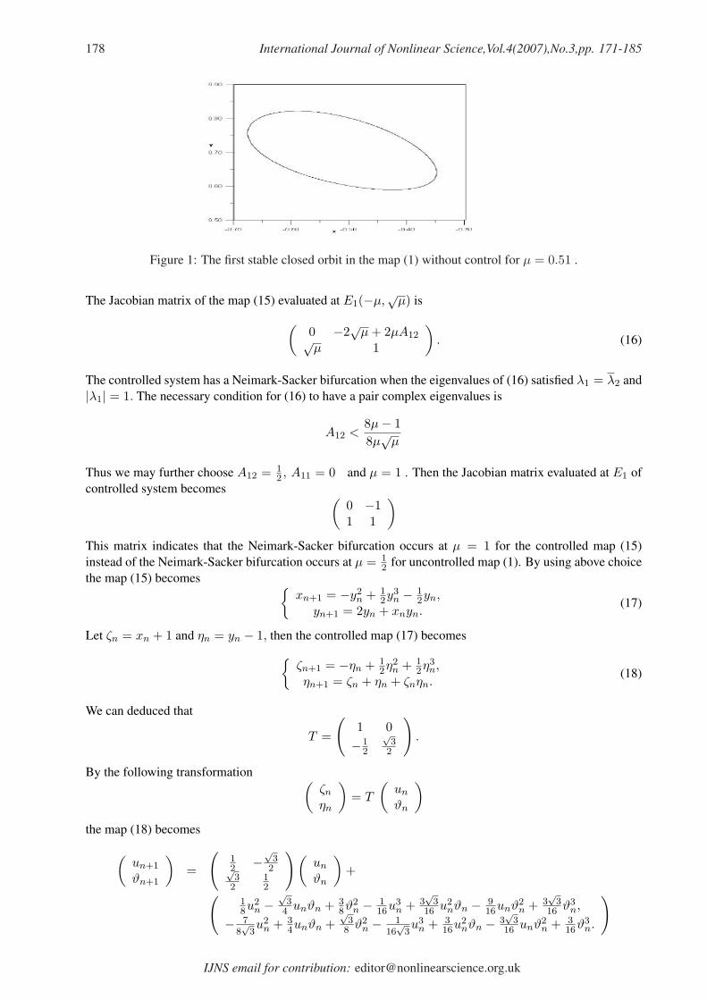
In this section we applied the same technique [4] to control our map about Neimark-Sacker bifurcation.As deduced by proposition that a stable Neimark-Sacker bifurcation occurs at µ = 0.5 . It is clear that, astable closed orbit in the phase space( see Figure 1).

Based on the above work, we may choose control component for first equation of the map (1). We canexplicitly write the controller as

kn = A11xn(xn + µ)2 + A12yn(y2n − µ2),

which preserves the three fixed points of the map (1). Then the controlled system given by xn+1 = −y2

n + A11xn(xn + µ)2 + A12yn(y2n − µ2),

yn+1 = (1 + µ)yn + xnyn.(15)



Figure 1: The first stable closed orbit in the map (1) without control for µ = 0.51 .

The Jacobian matrix of the map (15) evaluated at E1(−µ,√

µ) is

(0 −2

√µ + 2µA12√

µ 1

). (16)

The controlled system has a Neimark-Sacker bifurcation when the eigenvalues of (16) satisfied λ1 = λ2 and|λ1| = 1. The necessary condition for (16) to have a pair complex eigenvalues is

A12 <8µ− 18µ√

µ

Thus we may further choose A12 = 12 , A11 = 0 and µ = 1 . Then the Jacobian matrix evaluated at E1 of

controlled system becomes (0 −11 1

)

This matrix indicates that the Neimark-Sacker bifurcation occurs at µ = 1 for the controlled map (15)instead of the Neimark-Sacker bifurcation occurs at µ = 1

2 for uncontrolled map (1). By using above choicethe map (15) becomes {

xn+1 = −y2n + 1

2y3n − 1

2yn,yn+1 = 2yn + xnyn.

(17)

Let ζn = xn + 1 and ηn = yn − 1, then the controlled map (17) becomes

{ζn+1 = −ηn + 1

2η2n + 1

2η3n,

ηn+1 = ζn + ηn + ζnηn.(18)

We can deduced that

T =

(1 0−1

2

√3

2

).

By the following transformation (ζn

ηn

)= T

(un

ϑn

)

the map (18) becomes

(un+1

ϑn+1

)=

(12 −

√3

2√3

212

)(un

ϑn

)+

(18u2

n −√

34 unϑn + 3

8ϑ2n − 1

16u3n + 3

√3

16 u2nϑn − 9

16unϑ2n + 3

√3

16 ϑ3n,

− 78√

3u2

n + 34unϑn +

√3

8 ϑ2n − 1

16√

3u3

n + 316u2

nϑn − 3√

316 unϑ2

n + 316ϑ3

n.

)



Note that (15) is exactly in the form on the center manifold. By simple computation and using Eq. (4), wehave

γ20 =1

8√

3(√

3− i); γ11 =1

4√

3(√

3− i); γ02 = − 14√

3(√

3 + 2i); γ21 = −√

38

i.

Thus, l = − 132 < 0.

Figure 2: The first stable closed orbit in the controlled map (18) for µ = 1.1 .

Since l < 0 , the Neimark-Sacker bifurcation of the controlled map is a stable. The numerical simulationresult is shown in Figure 2, confirming the existence of a stable closed orbit in the phase space. From aboveanalysis, we deduce that the feedback controller polynomial function delays the appearance of Neimark-Sacker bifurcation and control the map around stable closed orbit.

4 Numerical Simulations

In this section, some numerical simulation results are presented to confirm the previous analytic results andto obtain even more dynamics behaviors of the map (1). To do this, we will use the bifurcation diagrams,phase portraits, Lyapunov exponents and Sensitive dependence on initial conditions and show the new in-teresting complex dynamical behaviors. The bifurcation parameters are considered in the following threecases :

(i) varying µ in range 0 ≤ µ < 1, and fixing ν = 1.

(ii) varying µ in range 0 ≤ µ < 1, and fixing ν = 2.

(iii) varying µ in range 0 ≤ µ < 1, and fixing ν = 0.5.

For case (i). Let ν = 1, the bifurcation diagram of x with respect to µ is presented in Figure 3. ThisFigure shows that the pitchfork bifurcation occurs at µ = 0, i.e., with the increase of the parameter µ, thestable fixed point E0(0, 0) loses its stability at µ = 0. When ν = 1, µ = 1

2 , according to the theoreticalanalysis given in section 2.2 , a Neimark-Sacker bifurcation should occur. This result has been proved bythe numerical simulation is shown in Figure 3.

We give the bifurcation diagram of the map (1) with ν = 1 in (µ−y) plane covering range µ ∈ [0, 0.99]in Figure 4 and the local amplification for µ ∈ [0.68, 0.72] in Figure 5 . Infact, the fixed points E1 and E2

of the map (1) losetheir stability at Neimark-Sacker bifurcation value at µ = 12 , so there is appearing of an

invariant circles when µ ≥ 12 .

Figures 3-5 show the dynamical behaviors of the map (1) become complex when the parameter µ > 12 .

Lyapunov exponents measure the exponential rates of convergence or divergence, in time, of adjacent trajec-tories in phase space. In order to analyze the parameter sets for which stable, periodic and chaotic behavior,one can compute the maximal Lyapunov exponents depend on µ . For the stable fixed points the maximalLyapunov exponents is negative. For quasiperiodic, invariant closed curve the maximal Lyapunov expo-nents is zero. For chaotic behavior the maximal Lyapunov exponents is positive. The maximal Lyapunovexponents corresponding to Figures 3-4 computed and presented in Figure 6.



Figure 3: Bifurcation diagram in(µ− x) plane for ν = 1.

Figure 4: Bifurcation diagram in(µ− y) plane for ν = 1.

Figure 5: Local amplificationcorresponding to 3.

Figure 6: Maximal Lyapunov exponents corresponding to Fig.3 and 4.

From Figure 6, one can see that the maximal Lyapunov exponents is in neighborhood of zero for µ ∈ [0, .65],which corresponds to fixed points or continuous closed invariant circles. When µ ∈ (0.65, 1) the maximalLyapunov exponents is positive which corresponding to chaotic behavior.For case (ii). The bifurcation diagram of map (6.1) in ( µ− y) plane for ν = 2 is shown in Figure 6.7. Thebifurcation diagram of the map (1) in ( µ− x) plane for ν = 2 is disposed in Figure 8. From this figure itsclear that the flip bifurcation emerges from the fixed point (−0.5, 1).

The maximal Lyapunov exponents corresponding to Figures 7, 8 is given in Figure 9, showing the periodorbits and the existence of chaotic regions as the parameter µ varying.

Case (iii), The bifurcation diagram of the map (1) in ( µ − x) plane for ν = 0.5 is plotted in Figure10, Also maximal Lyapunov exponents is disposed in Figure 10. The Neimark-Sacker bifurcation emergesfrom the fixed points (−0.5, 0.5) at ν = 0.5. It shows the correctness of Proposition 7.

From proposition 7, we deduced that the first Neimark-Sacker bifurcation takes place for µ = 12 and for

Figure 7: Bifurcation diagram in(µ− y) plane for ν = 2.

Figure 8: Bifurcation diagram in(µ− x) plane for ν = 2.

Figure 9: Maximal Lyapunovexponents corresponding toFig.7 and 8.



Figure 10: Bifurcation diagram in (µ − x) plane for ν = 0.5 and corre-sponding Maximal Lyapunov exponents .

Figure 11: The first Neimark-Sacker bifurcation when µ =0.5 .

Figure 12: The invariant closedcurve around the fixed point E1

created after Neimark-Sackerbifurcation when µ = 0.52 .

Figure 13: The breakdown ofthe invariant closed curve whenµ = 0.7 .

values lower than µ = 12 a stable fixed points exists. For µ = 1

2 and ν = 1 the fixed point E1 occurs at

x = −12 , y = 0.707 and the associated pair of complex conjugate eigenvalues are λ1,2 = 1

2 ±√

32 i with

|λ1,2| = 1, which shows that the first Neimark-Sacker bifurcation occurs at µ = 12 as shown in Figure. 11.

Continuing to increase the value of µ , we see what happens for µ = 0.52 and ν = 1 . One can see thatthe fixed point E1 became unstable and an invariant closed curve was created around the fixed point E1, asshown in the Figure 12.

The breakdown of the invariant closed curve around the fixed point E1 when µ = 0.7 and ν = 1 shownin Figure 13.

Further increases in µ the chaotic attractors arises. A typical double chaotic attractors presented inFigure 14, with µ = 0.83 and ν = 1, one chaotic attractor around fixed point E1 and the other one is aroundE2 .

In addition, Figure 15 shows more complex double chaotic attractorswith µ = 0.88 and ν = 1 .When µ = 0.9999 and ν = 1, invariant disc will appear due to a contact bifurcation between the attractor

and its basin boundary see Figure 16. The invariant disc disappear when µ = 1 . From Figure 16 its clearthat the existence of an invariant circle and invariant absolutely continuous measure on the disc boundedby this circle. It is true that the measure of the whole disc is infinitely large because the correspondingdensity is nonintegrable, the integral of this density logratithmicaly diverges near the boundary. In computersimulation, one can observe the longtime walking of iterations on the disc, but later all of them leave thedisc and go to infinity. This caused by transverse instability of the invariant boundary circle. It followsparticularly from the existence of unstable fixed points (0, 0) , (−1,±1) (and others unstable cycles) on itsboundary. After iterates arrive in a sufficiently small vicinity of such unstable fixed point or cycle they leavethe disc with a good probability because of round-of errors, see V. Tsybulin and V. Yudovich [17].

At ν = 1.5, the phase portraits corresponding to µ = 0.45, 0.5, 0.6, 0.75, and 0.85 are shown in Figure17(1)-(5) respectively. We see that the fixed points of the map (1) are stable for µ < 0.5 , and loses stabilityat µ = 0.5, an invariant closed curve appears when the parameter µ exceeds 0.5 . There is an invariant



Figure 14: Double chaotic at-tractor when µ = 0.83 .

Figure 15: Double chaotic at-tractor when µ = 0.88 .

Figure 16: Invariant disc(fulldeveloped chaos) when µ =0.999 .

closed curve for more large regions of µ ∈ (0.5, 0.72). When µ increases there are orbits of higher orderand attracting chaotic sets.

(a) (b)

(c) (d)

(e)

Figure 17: Phase portraits for various values of µ when ν = 1.5 .

In Figure 18, we see three typical chaotic attractors of the map (1) associated with the three cases (i)-(iii).

From above analysis one can deduce that Burgers mapping contains very rich nonlinear dynamics whenits parameters are varied. Many forms of complexities are observed such as chaotic bands (including peri-odic windows, pitchfork bifurcation, flip bifurcation, Neimark-Sacker bifurcation and attractors crisis) andchaotic attractors.



(a) (b)

(c)

Figure 18: Phase portraits for various values of ν when µ = 0.78 .

4.1 Sensitive dependence on initial conditions

To demonstrate the sensitivity to the initial conditions of the Burgers mapping, two orbits with initial points(x0 , y0) and (x0 +0.0001, y0) are computed, respectively,and are represented in Figure 19. At the beginning,the two time series are overlapped and are undistinguishable; but after a number of iterations, the differencebetween them builds up rapidly. Fig. 19 shows a sensitive dependence on initial conditions for x− coordinateof the two orbits for the model (1), which is plotted against the time with the parameter value µ = 0.73 andν = 2. The difference between the two x− coordinates is 0.0001 , while the other coordinate is kept to hasthe same value. For this case the two orbits with initial points (−0.04, 0.2) and (−0.0401, 0.2) are computedrespectively and plotted in Figure 19 as a function of time.

Figure 19: Sensitive dependence on initial conditions for map (1),x-coordinates of the two orbits,plottedagainst time;the x-coordinates of initial condition differ by 0.0001,and the other coordinate kept equal.

Also, the sensitive dependence on initial conditions, y− coordinates of the two orbits, for the map (1), areplotted against the time in Figure 20. The y− coordinate of initial conditions differs by 0.0001 ,while the



Figure 20: Sensitive dependence on initial conditions for map(1),y-coordinates of the two orbits,plottedagainst time;the y-coordinates of initial condition differ by 0.0001,and the other coordinate kept equal.

other coordinate is kept at the same value. From Figures 19 and 20 it is shown that the time series of themap (1) is a sensitive dependence to initial conditions, i.e. complex dynamic behaviors occur in this map.

5 Conclusions

In this paper, we have analyzed the dynamical behaviors for Burgers mapping map in R2 , and found manycomplex and interesting dynamical behaviors. Our theoretical analysis have demonstrated that the map (1)undergoes pitchfork bifurcation, flip bifurcation and Neimark-Sacker bifurcation. We controlled the maparound stable Neimark-Sacker bifurcation by using feedback polynomial controller method. Numericalsimulations carried out to verify our theoretical analysis.

Acknowledgments

One of us ( A. Elsadany) thanks Z. J. Jing, Y. Zhang and H. Cao for sending their some works papers.

References

[1] J. M. Burgers: Mathematical examples illustrating relations occurring in the theory of turbulent fluidmotion.Trans. Roy. Neth. Acad. Sci. Amsterdam. 17:1-53(1939)

[2] R. R. Whitehead, N. MacDonald: Introducing students to nonlinearity: computer experiments withBurgers mappings. Eur. J. Phys. 6:143-147(1985)

[3] R. R. Whitehead, N. MacDonald: A chaotic map that displays its own homoclinic structure.PhysicaD. 13:401-408(1984)

[4] Z. Chen, P. Yu: Controlling and anti-controlling Hopf bifurcations in discrete maps using polynomialfunctions.Chaos, Solitons & Fractals. 26:1231-1248(2005)

[5] Z. J. Jing, Z. Jia, R. Wang: Chaos bihavior in the discrete BVP oscillator. Int J Bifurcat& Chaos.12:619-627(2002)

[6] Z. J. Jing, Y. Chang, B. Guo: Bifurcation and chaos discrete FitzHugh-Nagumo system. Chaos &Solitons & Fractals. 21: 701-720(2004)

[7] Z. J. Jing, J. Yang: Bifurcation and chaos discrete-time predator-prey system. Chaos & Solitons &Fractals. 27: 259-277(2006)

[8] H. Sun, H. Cao: Bifurcations and chaos of a delayed ecological model.Chaos, Solitons & Fractals.4:1383-1393(2007)



[9] Y. Zhang, Q. Zhang, L. Zhao, C. Yang: Dynamical behaviors and chaos control in a discrete functionalresponse model. Chaos, Solitons & Fractals.4:1318-1327(2007)

[10] G. Iooss: Bifurcation of maps and applications. North-Holland, Amsterdam. (1977)

[11] Y. Chang, X. Li: Dynamical behaviors in a two-dimensional map. Acta Math App Sinica Engl Ser. 19:663-676(2003)

[12] Y.H. Wan: Computation of the stability condition for the Hopf bifurcation of diffeomorphism on R2.SIAM. J. Appl. Math. 34:167-175(1978)

[13] J. Guckenheimer, P. Holmes: Nonlinear oscillations, dynamical systems, and bifurcations of vec-tors.New York: Springer-Verlag.( 1983)

[14] K.C. Yap, GR. Chen, T. Ueta: Controlling bifurcations of discrete maps. latin Amer Appl Res. 31:157-162(2001)

[15] E.H. Abed, J.H. Fu: Local feedback stabilization and bifurcation control. I. Hopf bifurcation. SystContr Lett 7:11-17(1986)

[16] E.H. Abed, H.O. Wang, GR. Chen: Stabilization of period doubling bifurcations and implications forcontrol of chaos. Physica D. 70:150-164(1994)

[17] V. Tsybulin, V. Yudovich: Invariant setes and attractors of quadratic mapping of plane computer ex-periment and anlytical treatment.Int. J. Difference Equations and Applications. 4: 397-324(1998)


bifurcation analysis, chaos and control in the burgers mapping

Documents