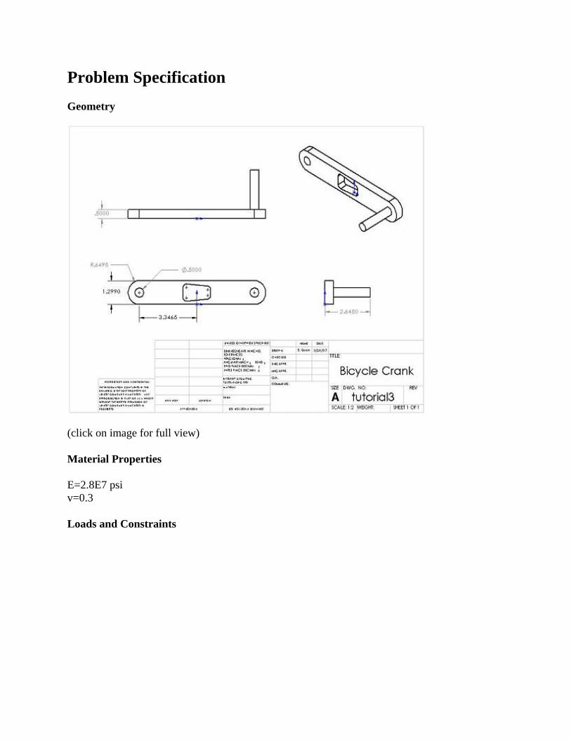
Problem Specification Geometry

(click on image for full view)

Material Properties

E=2.8E7 psi v=0.3

Loads and Constraints

Step 1: Start-up and preliminary set-up Create a folder

Create a folder called crank at a convenient location. We'll use this folder to store files created during the ANSYS session.

Start ANSYS

Start > Programs > Lab Apps > ANSYS 10.0 > ANSYS Product Launcher

In the window that comes up, enter the location of the folder you just created as your Working directory by browsing to it. All files generated during the ANSYS run will be stored in this directory.

Specify crank as your Initial jobname. The jobname is the prefix used for all files generated during the ANSYS session. For example, when you perform a save operation in ANSYS, it'll store your work in a file called plate.db in your working directory.

For this tutorial, we'll use the default values for the other fields. Click on Run. This brings up the ANSYS interface. To make best use of screen real estate, move the windows around and resize them so that you approximate this screen arrangement. This way you can read instructions in the browser window and implement them in ANSYS.

You can resize the text in the browser window to your taste and comfort.

In Internet Explorer: Menubar > View > Text Size, then choose the appropriate font size.

In Netscape: Menubar > View > Increase Font or Menubar > View > Decrease Font.

Set Preferences

As before, we'll more or less work our way down the Main Menu.

Main Menu > Preferences

In the Preferences for GUI Filtering dialog box, click on the box next to Structural so that a tick mark appears in the box. Click OK.

Recall that this is an optional step that customizes the graphical user interface so that only menu options valid for structural problems are made available during the ANSYS session.

Step 2: Specify element type and constants Specify Element Type

Main Menu > Preprocessor> Element Type > Add/Edit/Delete > Add...

Pick Structural Mass Solid in the left field and Brick 8node 45 in the right field. This is the mesh element we will be using to obtain our solution. Click Apply to select this element.

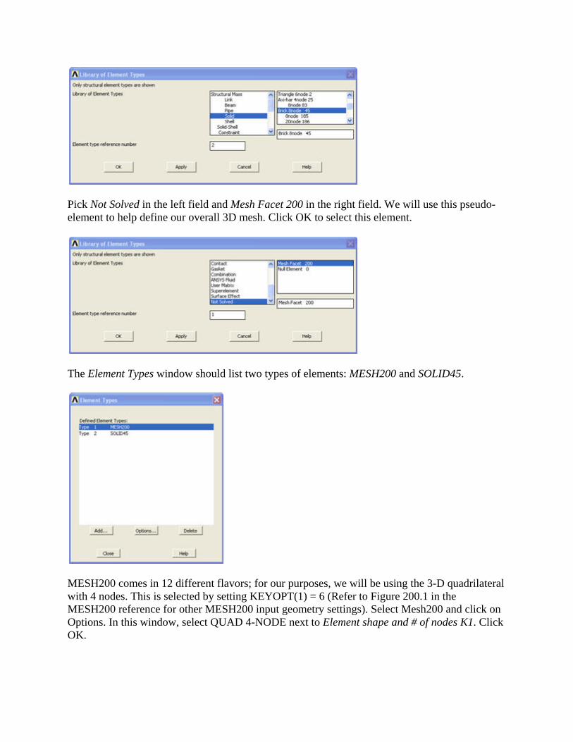
Pick Not Solved in the left field and Mesh Facet 200 in the right field. We will use this pseudo-element to help define our overall 3D mesh. Click OK to select this element.

The Element Types window should list two types of elements: MESH200 and SOLID45.

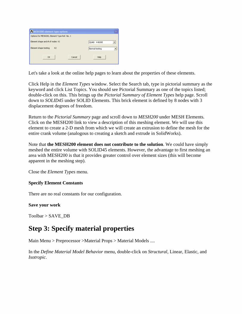
MESH200 comes in 12 different flavors; for our purposes, we will be using the 3-D quadrilateral with 4 nodes. This is selected by setting KEYOPT(1) = 6 (Refer to Figure 200.1 in the MESH200 reference for other MESH200 input geometry settings). Select Mesh200 and click on Options. In this window, select QUAD 4-NODE next to Element shape and # of nodes K1. Click OK.

Let's take a look at the online help pages to learn about the properties of these elements.

Click Help in the Element Types window. Select the Search tab, type in pictorial summary as the keyword and click List Topics. You should see Pictorial Summary as one of the topics listed; double-click on this. This brings up the Pictorial Summary of Element Types help page. Scroll down to SOLID45 under SOLID Elements. This brick element is defined by 8 nodes with 3 displacement degrees of freedom.

Return to the Pictorial Summary page and scroll down to MESH200 under MESH Elements. Click on the MESH200 link to view a description of this meshing element. We will use this element to create a 2-D mesh from which we will create an extrusion to define the mesh for the entire crank volume (analogous to creating a sketch and extrude in SolidWorks).

Note that the MESH200 element does not contribute to the solution. We could have simply meshed the entire volume with SOLID45 elements. However, the advantage to first meshing an area with MESH200 is that it provides greater control over element sizes (this will become apparent in the meshing step).

Close the Element Types menu.

Specify Element Constants

There are no real constants for our configuration.

Save your work

Toolbar > SAVE_DB

Step 3: Specify material properties Main Menu > Preprocessor >Material Props > Material Models ....

In the Define Material Model Behavior menu, double-click on Structural, Linear, Elastic, and Isotropic.

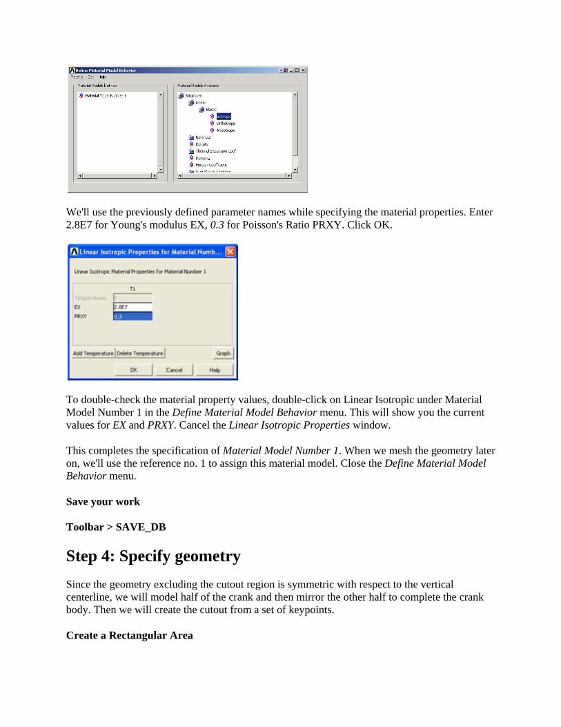
We'll use the previously defined parameter names while specifying the material properties. Enter 2.8E7 for Young's modulus EX, 0.3 for Poisson's Ratio PRXY. Click OK.

To double-check the material property values, double-click on Linear Isotropic under Material Model Number 1 in the Define Material Model Behavior menu. This will show you the current values for EX and PRXY. Cancel the Linear Isotropic Properties window.

This completes the specification of Material Model Number 1. When we mesh the geometry later on, we'll use the reference no. 1 to assign this material model. Close the Define Material Model Behavior menu.

Save your work

Toolbar > SAVE_DB

Step 4: Specify geometry Since the geometry excluding the cutout region is symmetric with respect to the vertical centerline, we will model half of the crank and then mirror the other half to complete the crank body. Then we will create the cutout from a set of keypoints.

Create a Rectangular Area

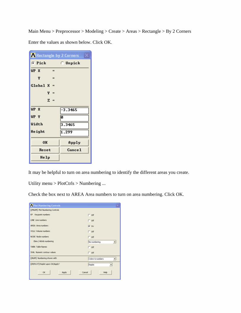
Main Menu > Preprocessor > Modeling > Create > Areas > Rectangle > By 2 Corners

Enter the values as shown below. Click OK.

It may be helpful to turn on area numbering to identify the different areas you create.

Utility menu > PlotCtrls > Numbering ...

Check the box next to AREA Area numbers to turn on area numbering. Click OK.

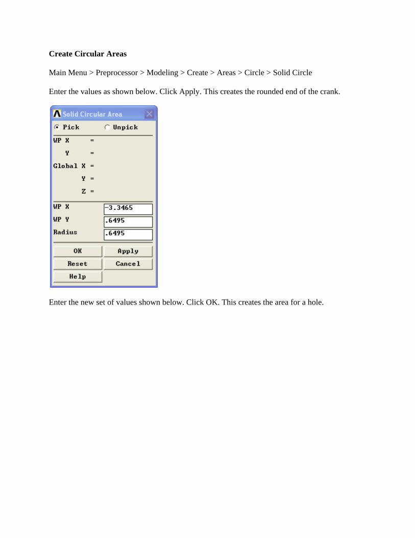
Create Circular Areas

Main Menu > Preprocessor > Modeling > Create > Areas > Circle > Solid Circle

Enter the values as shown below. Click Apply. This creates the rounded end of the crank.

Enter the new set of values shown below. Click OK. This creates the area for a hole.

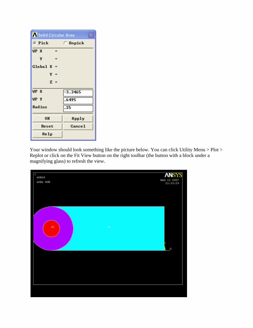
Your window should look something like the picture below. You can click Utility Menu > Plot > Replot or click on the Fit View button on the right toolbar (the button with a block under a magnifying glass) to refresh the view.

To correct any mistakes, you must click Main Menu > Preprocessor > Modeling > Delete > Areas Only and then pick each area you want to remove. The mouse pointer will show an up arrow for picking areas and a down arrow for un-picking areas. Right-click to switch between pick and unpick mode. When you have made all your selections, click OK. Click Utility Menu > Plot > Replot to refresh the view.

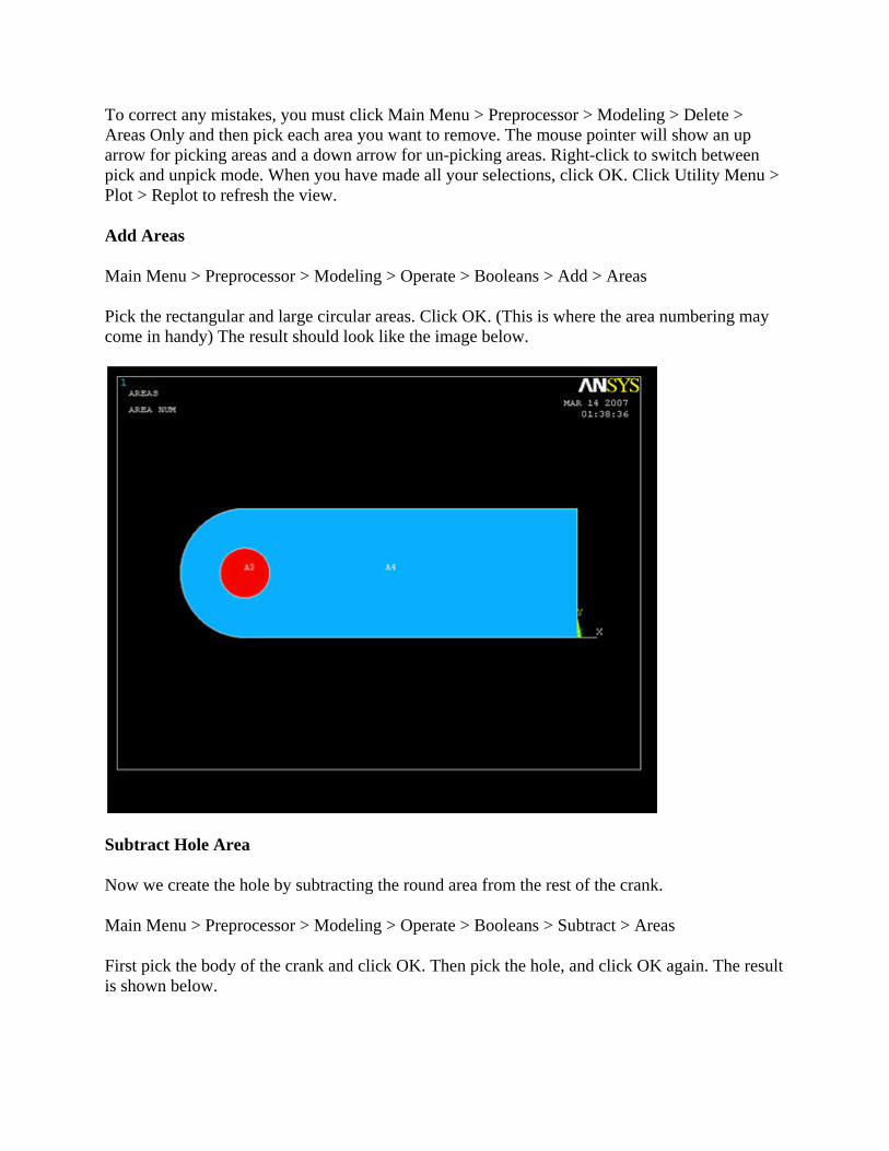
Add Areas

Main Menu > Preprocessor > Modeling > Operate > Booleans > Add > Areas

Pick the rectangular and large circular areas. Click OK. (This is where the area numbering may come in handy) The result should look like the image below.

Subtract Hole Area

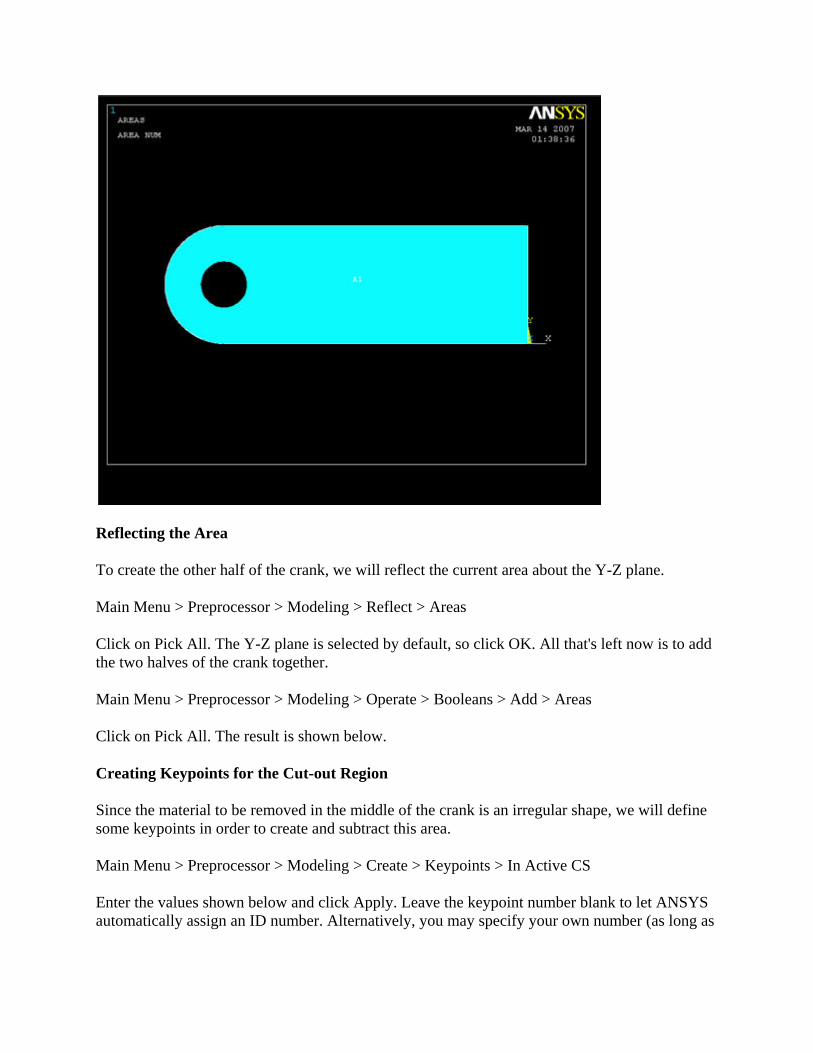
Now we create the hole by subtracting the round area from the rest of the crank.

Main Menu > Preprocessor > Modeling > Operate > Booleans > Subtract > Areas

First pick the body of the crank and click OK. Then pick the hole, and click OK again. The result is shown below.

Reflecting the Area

To create the other half of the crank, we will reflect the current area about the Y-Z plane.

Main Menu > Preprocessor > Modeling > Reflect > Areas

Click on Pick All. The Y-Z plane is selected by default, so click OK. All that's left now is to add the two halves of the crank together.

Main Menu > Preprocessor > Modeling > Operate > Booleans > Add > Areas

Click on Pick All. The result is shown below.

Creating Keypoints for the Cut-out Region

Since the material to be removed in the middle of the crank is an irregular shape, we will define some keypoints in order to create and subtract this area.

Main Menu > Preprocessor > Modeling > Create > Keypoints > In Active CS

Enter the values shown below and click Apply. Leave the keypoint number blank to let ANSYS automatically assign an ID number. Alternatively, you may specify your own number (as long as

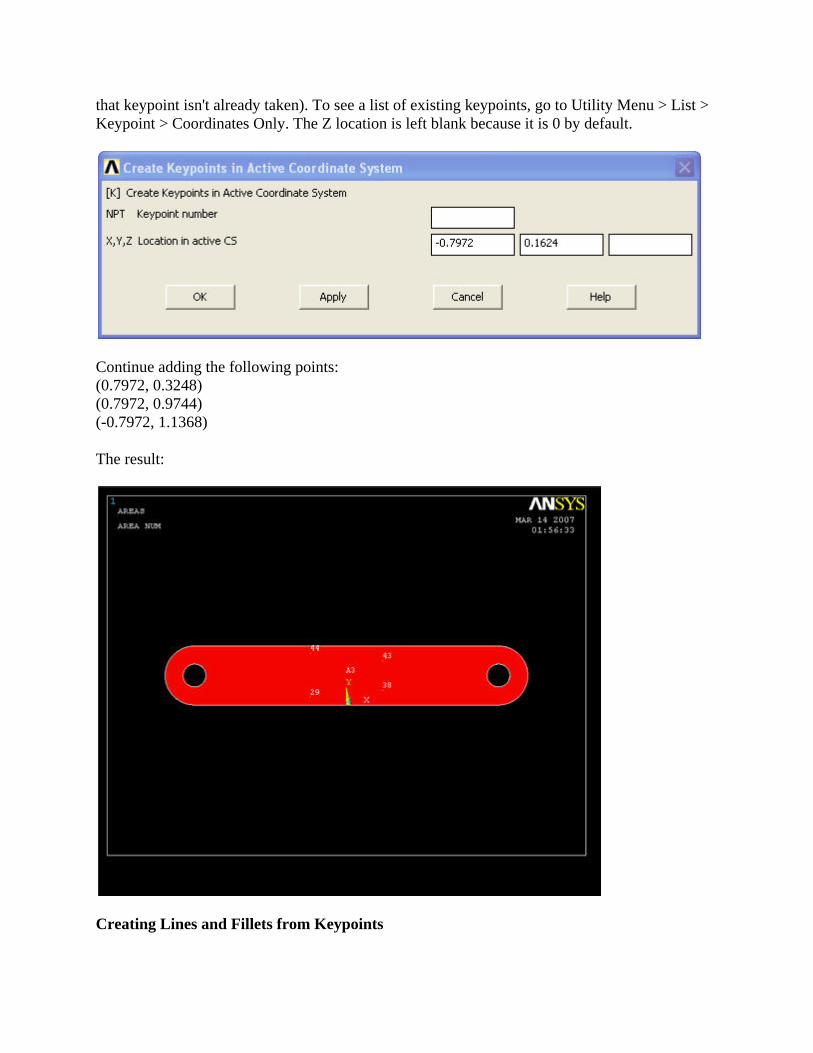
that keypoint isn't already taken). To see a list of existing keypoints, go to Utility Menu > List > Keypoint > Coordinates Only. The Z location is left blank because it is 0 by default.

Continue adding the following points: (0.7972, 0.3248) (0.7972, 0.9744) (-0.7972, 1.1368)

The result:

Creating Lines and Fillets from Keypoints

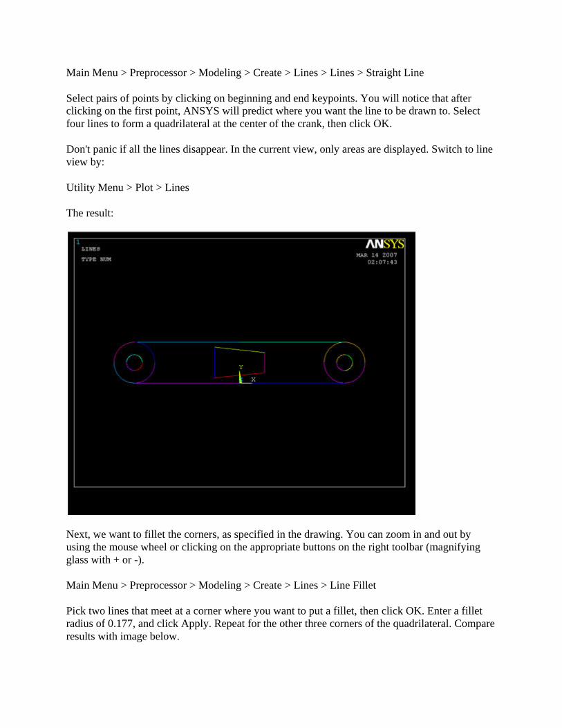
Main Menu > Preprocessor > Modeling > Create > Lines > Lines > Straight Line

Select pairs of points by clicking on beginning and end keypoints. You will notice that after clicking on the first point, ANSYS will predict where you want the line to be drawn to. Select four lines to form a quadrilateral at the center of the crank, then click OK.

Don't panic if all the lines disappear. In the current view, only areas are displayed. Switch to line view by:

Utility Menu > Plot > Lines

The result:

Next, we want to fillet the corners, as specified in the drawing. You can zoom in and out by using the mouse wheel or clicking on the appropriate buttons on the right toolbar (magnifying glass with + or -).

Main Menu > Preprocessor > Modeling > Create > Lines > Line Fillet

Pick two lines that meet at a corner where you want to put a fillet, then click OK. Enter a fillet radius of 0.177, and click Apply. Repeat for the other three corners of the quadrilateral. Compare results with image below.

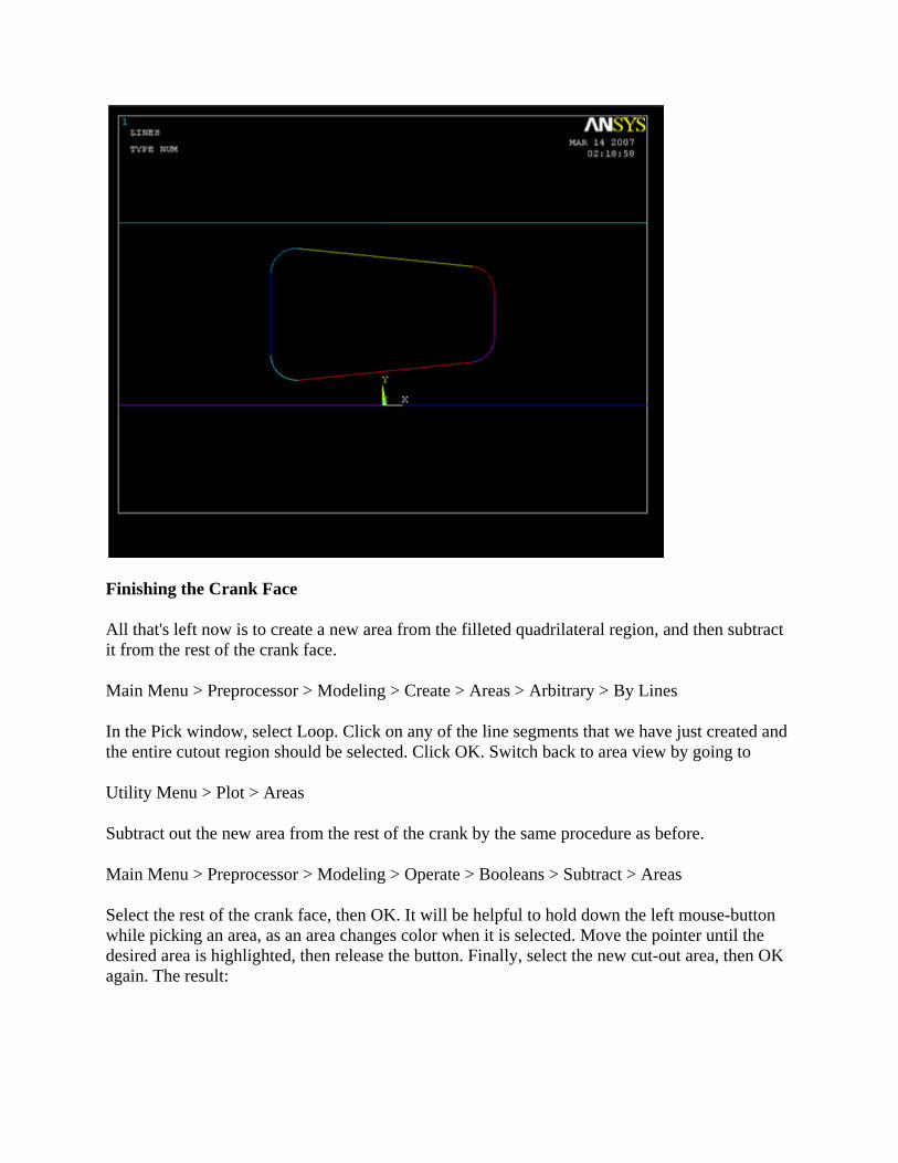
Finishing the Crank Face

All that's left now is to create a new area from the filleted quadrilateral region, and then subtract it from the rest of the crank face.

Main Menu > Preprocessor > Modeling > Create > Areas > Arbitrary > By Lines

In the Pick window, select Loop. Click on any of the line segments that we have just created and the entire cutout region should be selected. Click OK. Switch back to area view by going to

Utility Menu > Plot > Areas

Subtract out the new area from the rest of the crank by the same procedure as before.

Main Menu > Preprocessor > Modeling > Operate > Booleans > Subtract > Areas

Select the rest of the crank face, then OK. It will be helpful to hold down the left mouse-button while picking an area, as an area changes color when it is selected. Move the pointer until the desired area is highlighted, then release the button. Finally, select the new cut-out area, then OK again. The result:

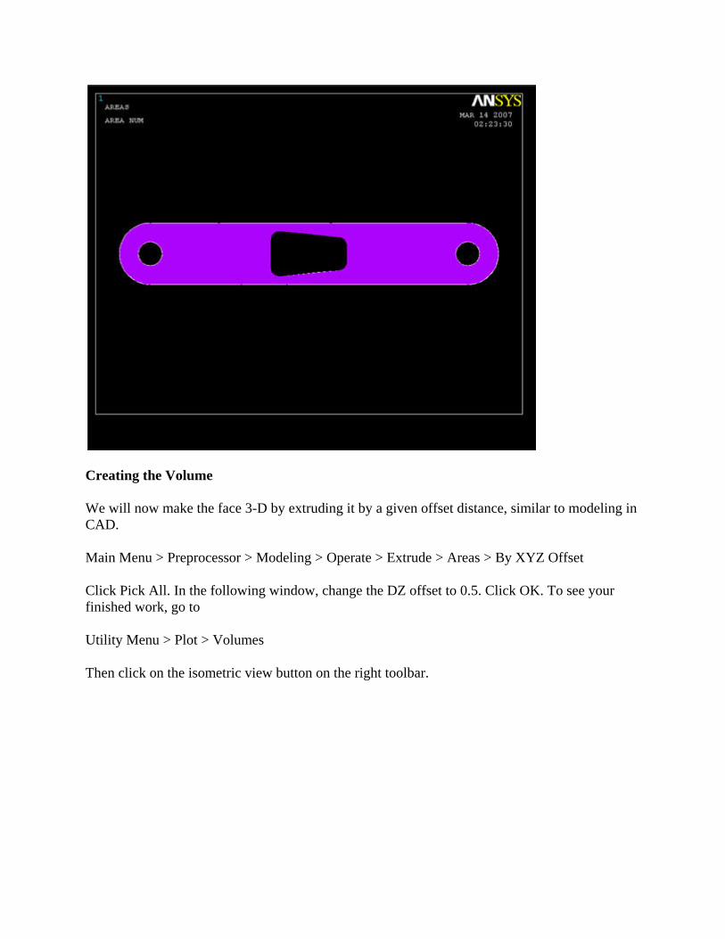
Creating the Volume

We will now make the face 3-D by extruding it by a given offset distance, similar to modeling in CAD.

Main Menu > Preprocessor > Modeling > Operate > Extrude > Areas > By XYZ Offset

Click Pick All. In the following window, change the DZ offset to 0.5. Click OK. To see your finished work, go to

Utility Menu > Plot > Volumes

Then click on the isometric view button on the right toolbar.

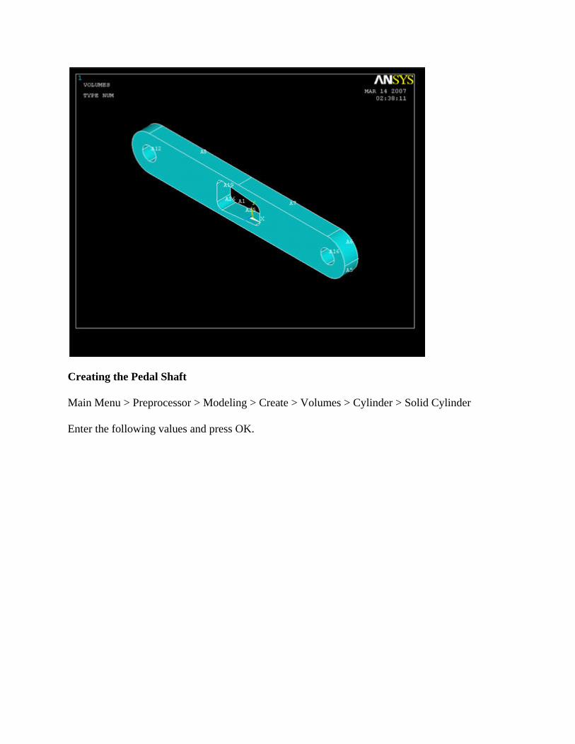
Creating the Pedal Shaft

Main Menu > Preprocessor > Modeling > Create > Volumes > Cylinder > Solid Cylinder

Enter the following values and press OK.

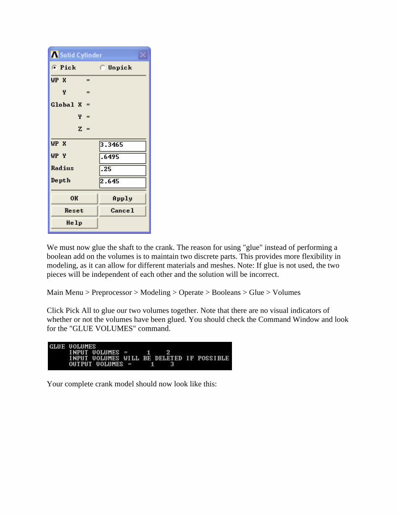
We must now glue the shaft to the crank. The reason for using "glue" instead of performing a boolean add on the volumes is to maintain two discrete parts. This provides more flexibility in modeling, as it can allow for different materials and meshes. Note: If glue is not used, the two pieces will be independent of each other and the solution will be incorrect.

Main Menu > Preprocessor > Modeling > Operate > Booleans > Glue > Volumes

Click Pick All to glue our two volumes together. Note that there are no visual indicators of whether or not the volumes have been glued. You should check the Command Window and look for the "GLUE VOLUMES" command.

Your complete crank model should now look like this:

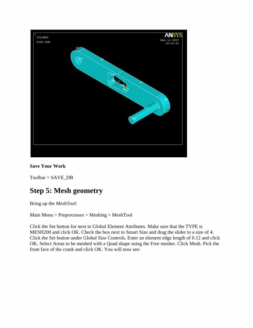
Save Your Work

Toolbar > SAVE_DB

Step 5: Mesh geometry Bring up the MeshTool:

Main Menu > Preprocessor > Meshing > MeshTool

Click the Set button for next to Global Element Attributes. Make sure that the TYPE is MESH200 and click OK. Check the box next to Smart Size and drag the slider to a size of 4. Click the Set button under Global Size Controls. Enter an element edge length of 0.12 and click OK. Select Areas to be meshed with a Quad shape using the Free mesher. Click Mesh. Pick the front face of the crank and click OK. You will now see:

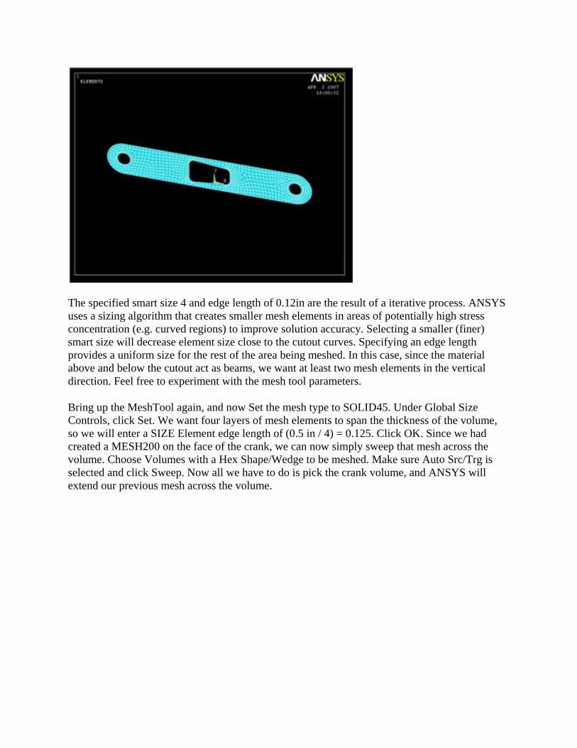
The specified smart size 4 and edge length of 0.12in are the result of a iterative process. ANSYS uses a sizing algorithm that creates smaller mesh elements in areas of potentially high stress concentration (e.g. curved regions) to improve solution accuracy. Selecting a smaller (finer) smart size will decrease element size close to the cutout curves. Specifying an edge length provides a uniform size for the rest of the area being meshed. In this case, since the material above and below the cutout act as beams, we want at least two mesh elements in the vertical direction. Feel free to experiment with the mesh tool parameters.

Bring up the MeshTool again, and now Set the mesh type to SOLID45. Under Global Size Controls, click Set. We want four layers of mesh elements to span the thickness of the volume, so we will enter a SIZE Element edge length of (0.5 in / 4) = 0.125. Click OK. Since we had created a MESH200 on the face of the crank, we can now simply sweep that mesh across the volume. Choose Volumes with a Hex Shape/Wedge to be meshed. Make sure Auto Src/Trg is selected and click Sweep. Now all we have to do is pick the crank volume, and ANSYS will extend our previous mesh across the volume.

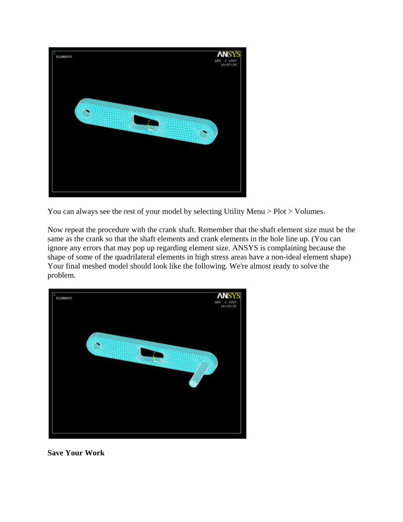
You can always see the rest of your model by selecting Utility Menu > Plot > Volumes.

Now repeat the procedure with the crank shaft. Remember that the shaft element size must be the same as the crank so that the shaft elements and crank elements in the hole line up. (You can ignore any errors that may pop up regarding element size. ANSYS is complaining because the shape of some of the quadrilateral elements in high stress areas have a non-ideal element shape) Your final meshed model should look like the following. We're almost ready to solve the problem.

Save Your Work

Toolbar > SAVE_DB

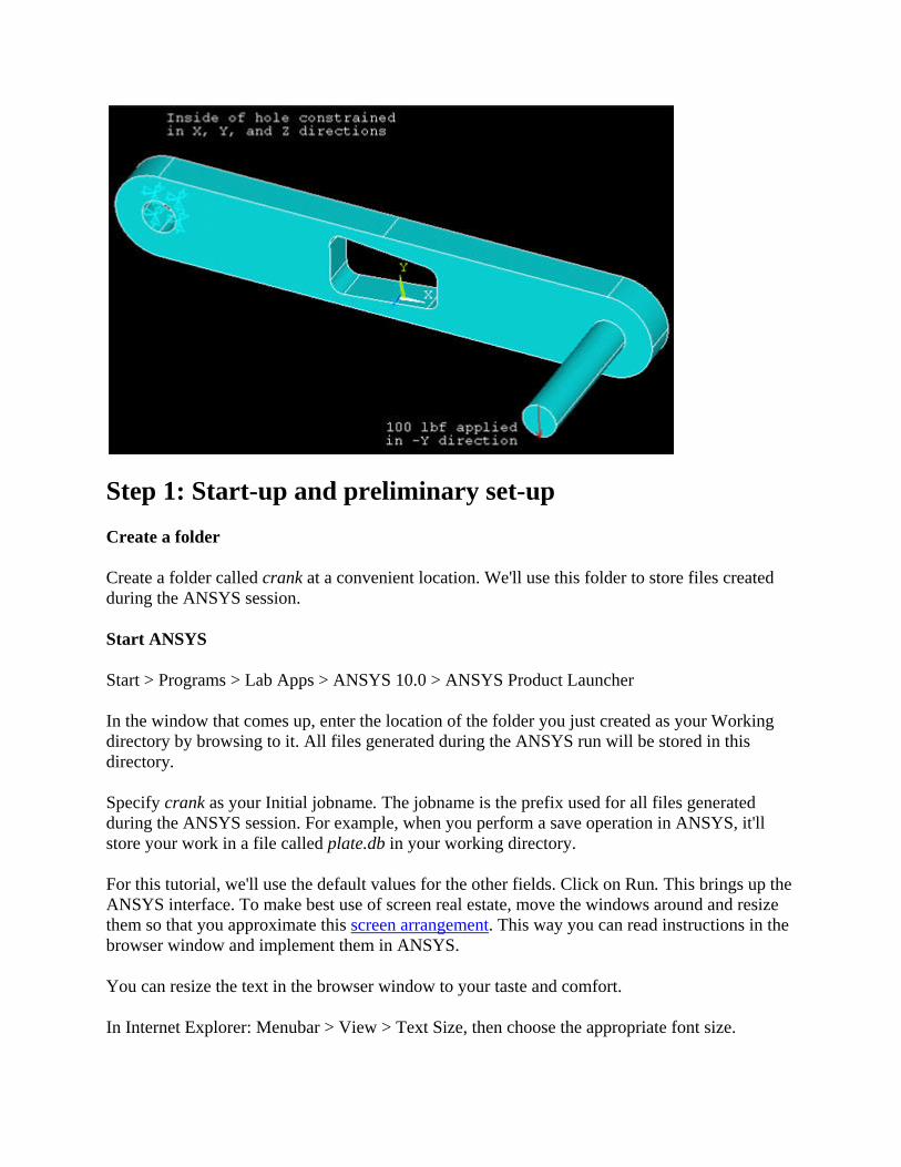
Step 6: Specify boundary conditions We have two loading conditions to specify. First we must fix the hole where the crank would attach to the bicycle. Then we apply our loading condition of 100 lb on the end of the shaft.

Fixed End

Main Menu > Preprocessor > Loads > Define Loads > Apply > Structural > Displacement > On Areas

It will be helpful to see the areas we're constraining, so select Utility Menu > Plot > Areas. We can see that the hole consists of multiple areas (4, in fact). Hold down the left-click and you can see that there are 4 surfaces that make up the inside of the hole. Pick all 4 and click OK. Select All DOF and click OK. The displacement value can be left blank as it defaults to 0. You can now see the displacement is fixed in 3 directions at four places.

Force on Shaft

Main Menu > Preprocessor > Loads > Define Loads > Apply > Structural > Force/Moment > On Keypoints

Select Utility Menu > PlotCtrls > Numbering ... and turn On Keypoint Numbers. Click OK. Notice that there is conveniently a keypoint at the tip of the shaft, and pick this point to apply the force. Click OK. From the orientation of our axes, we want a constant force in the FY direction with a value of -100. Click OK.

What the model looks like now:

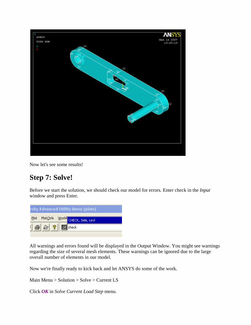
Now let's see some results!

Step 7: Solve! Before we start the solution, we should check our model for errors. Enter check in the Input window and press Enter.

All warnings and errors found will be displayed in the Output Window. You might see warnings regarding the size of several mesh elements. These warnings can be ignored due to the large overall number of elements in our model.

Now we're finally ready to kick back and let ANSYS do some of the work.

Main Menu > Solution > Solve > Current LS

Click OK in Solve Current Load Step menu.

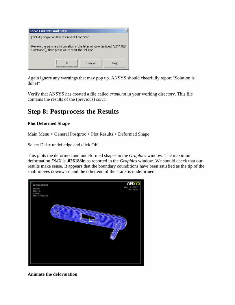
Again ignore any warnings that may pop up. ANSYS should cheerfully report "Solution is done!"

Verify that ANSYS has created a file called crank.rst in your working directory. This file contains the results of the (previous) solve.

Step 8: Postprocess the Results Plot Deformed Shape

Main Menu > General Postproc > Plot Results > Deformed Shape

Select Def + undef edge and click OK.

This plots the deformed and undeformed shapes in the Graphics window. The maximum deformation DMX is .026188in as reported in the Graphics window. We should check that our results make sense. It appears that the boundary counditions have been satisfied as the tip of the shaft moves downward and the other end of the crank is undeformed.

Animate the deformation

Utility Menu > PlotCtrls > Animate > Deformed Shape...

Select Def + undeformed and click OK. Select Forward Only in the Animation Controller.

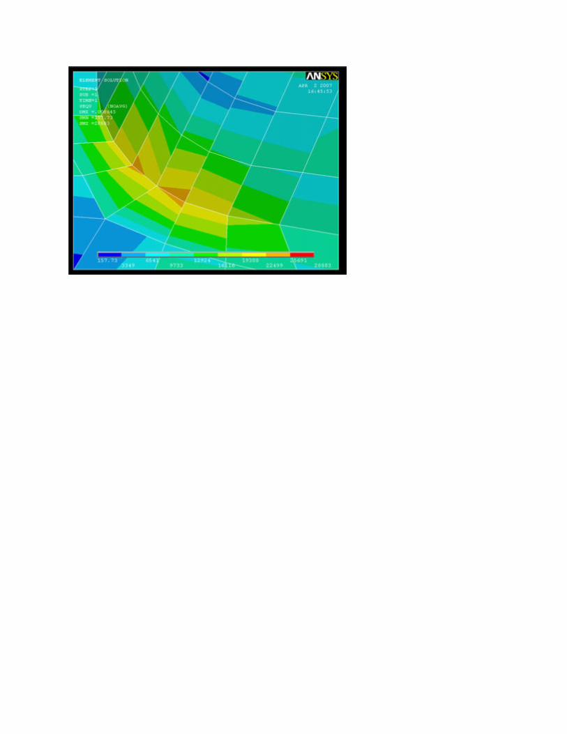
Plot Nodal Solution of von Mises Stress

Main Menu > General Postproc > Plot results > Contour Plot > Nodal Solu

For a quick refresher on von Mises stress, click Help. Search for von mises and click on the result 2.4 Combined Stresses and Strains. This can be useful if your MAE212 book isn't lying around.

Select Nodal Solution > Stress > von Mises stress and click OK. To change the range of stresses displayed, go to

Utility Menu > PlotCtrls > Style > Contours > Uniform Contours ...

and select User specified. Specify a range of minimum 0 and maximum 25000. We can now see more color variation in the model, and easily pick out the red areas.

When you plot the "Nodal Solution", ANSYS obtains a continuous distribution as follows: 1. It determines the average at each node of the values of all elements connected to the node. 2. Within each element, it linearly interpolates the average nodal value obtained in the previous step.

The stress concentration located at the tip of the shaft can be ignored as the force is applied as a point load. To hide the crank shaft, go to

Utility menu > Select > Entities ...

Select Volumes, By Num/Pick, From Full and click Apply. Pick the crank volume and click OK. After we've selected a volume, we must select all the elements in this volume to be plotted. In the Select Entities window, select Elements, Attached to, Volumes and click Apply. Click Replot to display the new selection. Notice the deformation is exaggerated, revealing that deformation is primarily caused by torsion.

To see the whole model again, go to the Select Entities window and click Sele All and Replot. (If for some reason select all fails, you can always go to Utility Menu > Select > Everything)

Comparing the Sigma_xx Stress with von Mises Stress

To verify that the bending stress in the crank is relatively insignificant, we can compare the element sigma_xx solution with the elemental von Mises solution.

General Postproc > Plot Results > Contour Plot > Element Solu

Click on Stress, then X-Component of stress , then the Apply. Notice that the top-left and bottom-right corners of the cutout area are now blue, and that the scale has been readjusted to show that blue is now a large negative stress value. If this were a case of pure bending, we would expect the top of the crank to be in tension, not compression! (Note: if grey areas are appearing in your contour plots, you should go to Utility Menu > PlotCtrls > Style > Contours > Uniform Contours ..., select Auto calculated, and click OK.)

To find out information about specific points on the model, go to

General Postproc > Query Results > Subgrid Solu

Select Stress, X-direction SX, and click OK. The picking window will appear, and you can click on any point in the model. Click OK when finished.

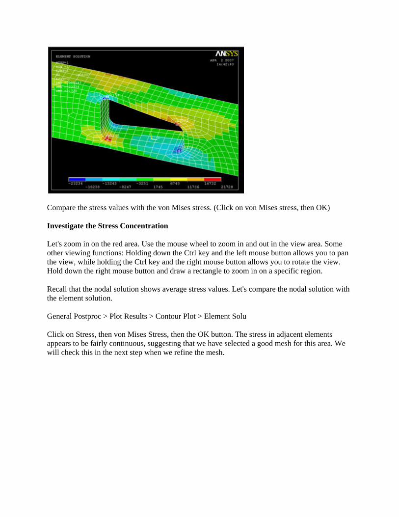
Compare the stress values with the von Mises stress. (Click on von Mises stress, then OK)

Investigate the Stress Concentration

Let's zoom in on the red area. Use the mouse wheel to zoom in and out in the view area. Some other viewing functions: Holding down the Ctrl key and the left mouse button allows you to pan the view, while holding the Ctrl key and the right mouse button allows you to rotate the view. Hold down the right mouse button and draw a rectangle to zoom in on a specific region.

Recall that the nodal solution shows average stress values. Let's compare the nodal solution with the element solution.

General Postproc > Plot Results > Contour Plot > Element Solu

Click on Stress, then von Mises Stress, then the OK button. The stress in adjacent elements appears to be fairly continuous, suggesting that we have selected a good mesh for this area. We will check this in the next step when we refine the mesh.