biases in computed returns an application to the size effect
TRANSCRIPT

Journal of Financial Economics 12 (1983) 387-404. North-Holland
BIASES IN C O M P U T E D RETURNS
An Application to the Size Effect*
Marshall E. BLUME University of Pennsylvania, Philadelphia, PA 19104, USA
Robert F. STAMBAUGH University of Pennsylvania, Philadelphia, PA 19104, USA
Received February 1983, final version received August 1983
Previous estimates of a 'size effect' based on daily returns data are biased. The use of quoted closing prices in computing returns on individual stocks imparts an upward bias. Returns computed for buy-and-hold portfolios largely avoid the bias induced by closing prices. Based on such buy-and-hold returns, the full-year size effect is half as large as previously reported, and all of the full-year effect is, on average, due to the month of January.
1. Introduction
Recent empirical work in finance reports that average risk-adjusted returns on stocks of small firms exceed those of large firms, where size is measured by the market value of outstanding common equity. 1 Using daily returns for stocks on both the New York and American Stock Exchanges, Reinganum (1982) finds that, during the 1964-1978 period, the average return for firms in the lowest market-value decile exceeds the average return for firms in the highest decile by more than 0.1 percent per day - - over 30 percent per year.
He also finds that various methods of risk adjustment contribute little towards explaining such impressive differences. 2 Keim (1983) reports that almost half of the annual difference between returns on small and large firms occurs in January.
The 'size effect' is particularly pronounced in the studies that use daily returns data, but we show that, due to a statistical bias, these studies significantly overstate the magnitude of the size effect. Although we
*We are grateful to Edwin Elton, Donald Keim, Jay Ritter, Hans Stoll, participants in workshops at New York University and Yale University, and the referee, Allan Kleidon, for comments and suggestions. The research assistance of Tzivia Kandel is gratefully acknowledged.
1See Blume and Friend (1974) and Banz (1981) for evidence on the size effect in addition to that discussed in the text.
2See also Reinganum (1981a, b).
0304~05x/83/$3.00 © 1983, Elsevier Science Publishers B.V. (North-Holland)

388 M.E. Blume and R.F. Stambaugh, Return computation and the size ~'[l~'et
empirically analyze the bias in the context of the size effect, the same bias could potentially occur in any study using closing prices to compute returns, particularly daily returns.
Using daily returns for NYSE and AMEX stocks, we find that (1) the average size effect over the entire year is about 0.05 percent per day only hal f as large as reported by Reinganum and Keim - - and (2) virtually all of this full-year average is attributable to January. In other words, the size effect averages about 0.60 percent per day in January and roughly zero in the remainder of the year. The sample contains all firms listed on the New York and American Stock Exchanges, and the time period covers 1963 through 1980. Thus, our study uses essentially the same data as prior studies.
The difference in results arises from the method used to compute average returns. Section 2 shows that single-period returns on individual stocks computed with recorded closing prices are upward biased. This bias arises from a 'bid ask' effect in closing prices and can be non-trivial for daily returns on stocks of small firms. Reinganum and Keim use arithmetic averages of daily returns to estimate the size effect. Since the arithmetic average of computed returns contains the average bias for the individual stocks, their estimates of the size effect are upward biased.
The portfolio strategy implicit in arithmetic averaging is one of daily rebalancing to equal weights. This paper shows that the returns on an alternative buy-and-hold strategy are virtually unbiased. Buy-and-hold portfolios contain a "diversification" effect, not present in rebalanced portfolios. This 'diversification" effect removes virtually all bias from the computed returns on a buy-and-hold portfolio.
Section 3 presents empirical results for both rebalanced portfolios and buy-and-hold portfolios. The differences between returns on the two strategies are negligible for large-firm portfolios. In contrast, for the portfolio of the lowest-market-value firms, the rebalanced return exceeds the buy-and- hold return by an average of 0.05 percent per day, which is approximately half of the average size effect reported in previous studies. The analysis in section 4 finds that the difference between the rebalanced and buy-and-hold returns varies inversely with share price, holding market wdue constant, and bears no significant relation to market value, holding share price constant. This finding is consistent with the analysis of the bias presented in section 2.
2. Computing returns with closing prices
2.1. A model o f closing prices
Define the true price at time t of stock i as Pi, , , the price at which, aside from transactions costs, a share of stock can be both bought and sold at a given time by placing a market order. On the Exchange, the true price can

M.E. Blume and R.F. Stambaugh, Return computation and the size q~]ect 389
be viewed as the price at which (nearly) simultaneous public market buy and sell orders would 'cross ' on the floor.
The Center for Research in Security Prices (CRSP) provides daily returns for stocks listed on the New York and American Stock Exchanges, and these returns are computed with 'closing' prices. The closing price is the price at which the last t ransaction occurred prior to the close of trading. 3 Let P~,, denote the reported closing price of stock i for the period ending at time t.
The closing price, P~.3, can deviate from the true price, Pz,,, if, for example, the last t ransaction reflects a public market order on only one side. For example, a market sell order might be matched with a limit buy order or bought by the specialist on his own account. Denote the price recorded for such transactions as a 'bid' price, and note that such a price is most likely less than the true price. Similarly, a market buy order that is not crossed on the floor results in the recording of an 'ask' price, probably greater than the true price. We refer to this property of closing prices as the bid-ask effect.
The bid-ask effect is modeled as
or
Pi,, =[1 +(~i,t]Pi,, , (1)
Pi,t = Pi,t-4-si,t, (1')
where E{6i , ,}=0, 61,~ is independently distributed across t, and 6i,t is independent of Pi,¢ for all r. At some points in the discussion, it will be convenient to use (1'), which is restated with an additive disturbance ei,t.
It is well-known that the b id-ask effect produces negative first-order autocovar iance in recorded price changes for individual stocks. 4 We show here that the b id-ask effect also imparts an upward bias to computed rates of return for individual stocks. 5 We analyze single-period returns primarily because most empirical studies employ single-period returns, often averaged either cross-sectionally or over time.
2.2. The bias in computed returns
The true return for security i for period t is defined, assuming no dividends
3If there are no trades in a day, CRSP uses as the quoted closing price the average of the bid and ask prices. To the extent that the bid and ask prices are kept up to date, this practice of CRSP could help reduce the differences between true and quoted prices.
4Niederhoffer and Osborne (1966) explain how the bid-ask effect leads to 'reversals', or negative autocorrelation in price changes.
SOur work is not without precedent, however. Although he does not consider the bid ask effect, Fisher (1966) discusses how deviations of closing prices from 'true' prices can bias computed returns.

390 M.E. Blume and R.F. Stambaugh, Return computation and the size ¢[]ect
for the period, as
Pi,t Fi, t = I.
Pi. t 1
The computed return is, using {I), defined as
El,, [1 +(Si , , ]Pi , , t : i ' t = P i . t 1 [ l+f i i . , 1]Pi., l
Combining (2) and (3} yields
l + 6 i t 6 . , - " [ l + r i , , ] - l .
1 + 6 i . ' I
Taking expectations of both sides of (4) gives
{2}
(3)
(4)
' ' { 1+6; ' t[~ ' ' + 1 = + E . ~ I / . , , ] - - 1. {5}
By Jensen's inequality, E{[1 +6~,,]/[1 +~¢., ~]}.> i. Therefore, E{r,,,}.
The bias can be approximated (using a Taylor series) as ~
E{,:;,,} >
E { r i . t } ~ E { v i , t } ~-(T2{()i,t 1}. {6)
where o-2{ } denotes the variance. If the third- and higher-ordered odd moments of (3i,t 1 are zero, then the variance term in (6) provides a lower bound for the bias induced by the bid ask effect.
2.3. The potential magnitude ol'the bid ask bias
To assess roughly the potential magnitude of the bid ask bias, denote the true price as P and assume that the closing period is either a bid price, PB, or an ask price, PA, with equal probability. Since the expected closing price is assumed equal to the true price. P must be (PB + PA)/2, and (~i is then either plus or minus (PA--PB)/2P. In this simple case, the bid-ask bias in (6) becomes
~,'i~ = + p~ (7)
"The first expecta t ion on the right side of {5) can be writ ten as E{I/{I+~5~., ~)I = E{I (5~., +6~. , . , - . . . }~l+aZ{f i i . , 11. C o m b i n i n g this with (5} and d ropp ing the cross product term gives (6). This a r g u m e n t requires 1 < ~ . , ~ < 1, that is. the closing price is greater than zero and less than twice the t rue price.

M.E. Blume and R.F. Stambaugh, Return computation and the size effect 391
Based on averages over 1963-1980, 'small' stocks - - those in the lowest decile of equity capitalization - - have an average price of about $5.00 per share and an average computed daily return of 0.141%. In order to assess the potential bias for such small stocks, we choose a single day at random, December 13, 1973, and select all NYSE common stocks with bid prices less than $8.00 per share. 7 This procedure gives 332 stocks with an average true price of $5.09, where true price is given by (PB+PA)/2. For each of these stocks we compute a2{61} using (7), and the average of these individual values is 0.051%. Thus, for small firms, a significant portion of their computed daily returns may reflect a bid-ask bias.
For the stocks of large firms, the bid-ask bias in (7) is likely to be negligible. Stoll and Whaley (1983) report that, for stocks in the highest equity-capitalization decile on the NYSE, bid-ask spreads average about 0.7~o of the 'true' price defined above. A stock with such a spread would have a value for a2{6i} of only 0.001~o.
2.4. Non-synchronous trading
Aside from the bid-ask effect, the closing price can deviate from the true price if the last transaction occurs before the end of the period. This problem, first analyzed by Fisher (1966), is generally referred to as 'non- synchronous trading' and, like the bid-ask effect, is known to produce negative autocovariance in returns. 8 Roll (1983) analyzes compounded returns in the context of this negative autocovariance. One can show that non-synchronous trading also imparts an upward bias to computed single- period returns. Under reasonable assumptions, however, the magnitude of the bias appears to be negligible compared to the bid-ask bias. 9
2.5. Rebalanced versus buy-and-hold portfolios
Many empirical studies, including those of the size effect, compute a portfolio return as the arithmetic average of the returns on individual
7Closing quotations of bid and ask prices are obtained from Stock Quotations on the New York Stock Exchange, a publication of Francis Emory Fitch.
8See Scboles and Williams (1977). 9The relative magnitudes of the biases can be analyzed within the framework used by Scholes
and Williams (1977). Assume the true price, P~.,, follows an infinitely divisible lognormal process with cti=ln[E{PL,/P~. , 1}]. Then the bias in the computed (simple) return is approximately ~2a2{s~.,}, where s~.t is the length of the period of non-trading prior to time t. Suppose ~= 1.4 × 10 -3 per day and s~.t takes values of either 0 or l with equal probability. Even in this extreme case, ct2tr2{s~.,} =4.9 × 10 -7, which is over 1000 times smaller than the potential bid-ask bias considered above.
Scholes and Williams also show that continuously compounded returns are unbiased, i.e., E{ln( l+i~, , )}=E{ln( l+rc , )} . It is easily seen that this is true with the bid-ask effect as well, since E{ln[( l+h~. , ) / ( l+fi i . t 1)]}=1 if it is further assumed that the 6~,,'s are identically distributed over time.

392 M.E. Blume and R.F. Stambaugh, Return computation and the size tT[]bet
securities. Since arithmetic averaging implies rebalancing to equal weights each period, this calculation gives the return on a rebalanced portfolio. The computed return on the rebalanced portfolio is thus biased by the average of bid-ask biases in the individual returns. That is, if the true rebalanced return is rRR,, = ( l / N ) E r i , t , and the computed return is fRR,, =( l /N) ~i i . , , then
2~. /Pi , }' t , - , (8)
where a bar indicates an average over i, and O'21(~i,t 1] in (6) is rewritten as iT~ ~ E i , t 1 / P i , t - I } using ( 1 ' ) .
The bid-ask bias can be greatly reduced by instead computing the return on a buy-and-hold portfolio. The buy-and-hold strategy invests an equal amount in each of N securities at an initial time 0, but no further transactions are performed. Assume all N stocks have the same initial price at time 0 and that no dividends are paid from time 0 through time t. Though not essential for the analysis, this assumption simplifies the notation in that numbers of shares need not appear explicitly in expressions for portfolio returns.
The true return for the buy-and-hold portfolio is given by
N
E Pi, t 1:1 1. (9)
F B H , t - - N
E Pi, , t i ~ l
The computed buy-and-hold return is
N N ~,'
2 & , Z e,.,+ 2 - i = I 1 ' = i ( = 1 - - - 1 . . . . 1 ( 1 0 ) FBH, t = N N N "
, 2 e , . , ,+E,:,., i = 1 i = I i = l
Rewriting (I 0), using (9), yields
1 +rllrl, t+F,t/Pt t " l ( l l ) r , . . , = l+g, l/P, i
The expectation of t:gn,, can be approximated [again using a Taylor series with (11)] as 1°
. } . (12)
~°First take the expectation of (10) conditional on Pt ~, the vector of true prices at t - l. Using a Taylor series, this can be written

M.E. Blume and R.F. Stambaugh, Return computation and the size effect 393
The bid-ask bias for the buy-and-hold return is reduced by a diversification effect. The bias in the rebalanced return in (8) is an average of variances of g~/Pi, or the average individual stock bias. The buy-and-hold bias in (12) is instead the variance of an average: the e~'s (and Pi's) are first averaged across stocks before computing the variance. The computed buy- and-hold portfolio return behaves like that of a security whose closing price deviates by ~ from its true price P~. For a portfolio of 100 stocks, with the occurrences of bids or asks independent across stocks, the average individual stock bias is about 100 times larger than the buy-and-hold bias.
An alternative way to view the reduction in the bias for the buy-and-hold return is as follows. The computed return on any portfolio can in general be written as i=~wii~, where wi is the proportion placed in asset i. The expected computed return is then
N N E{f}= E E{wi}E{f,}+ E cov{wi,fi}. (13)
i=1 i = 1
The first term on the right is a weighted average of computed individual returns and therefore contains the weighted average of the individual biases. For the buy-and-hold portfolio, the second term on the right of (13) offsets this bias, since the covariance between the weight and ?i is negative. I~ For the rebalanced portfolio, or for that matter any portfolio whose weights are contemporaneously uncorrelated with computed returns, the second term in (13) is zero, yielding no reduction in the bias.
The magnitude of the bid-ask bias can be assessed by examining the expected difference in computed returns on the two portfolio strategies. 12 Using (8) and (12),
E{ rRB - - ?~BH} ~ E{FRB - - ra i l} + [a2{ v.,/P, } - - o2 { ~ / P } ] , (14)
E{~.,,,,l_e, ,}~E(r. . , ,Lp ' ,}+~2{~,_,/p, ,le, ,}. Taking unconditional expectations then gives (11), noting
E[ff2{a,-l/P' l]_Pt-l}]=°'2{ ~ ̀ , / P t , since E{f.,_,/P, ,[P, t l = 0 for all P ,_ , .
lIRewrite {10) as
fun., = ~ {[P, . , - , +*;,.,- ,]/IN{P, , +.q ,)]}{{P,., + e,,)/(P,., , +e.,., ~)- 1}, i=1
where the first expression in braces equals w~ and the second expression in braces equals re. Recall from section 2.2 that the bias arises from e~.,_, in the denominator of fi (due to Jensen's inequality), which is now offset by el.,_ l in the numerator of wi. This offset produces a negative correlation between w i and il. As N grows large, ~,_, approaches zero and the reduction in the bias becomes complete.
' :See Roll {1983) for an analytical comparison of compounded returns on buy-and-hold and rebalanced portfolios in a two-period model.

394 M.E. Blume and R.F. Stambaugh, Return computation and the size e[]bct
where t ime indexes are suppressed to ease notat ion. The expected computed difference between reba lanced and buy -and -h o ld re turns equals (i) the expected difference in true re turns plus (it) the difference in the b i d - a s k biases. In general , E{rR~--r~3.}<0, since, if expected re turns differ across stocks, those with greater expected re turns receive a greater expected weight in the buy -and -ho ld por t fol io than in the reba lanced portfol io. ~3 In large portfol ios , the difference in b i d - a s k biases is close to the average individual securi ty (or r eba lanced portfol io) bias, since the b u y - a n d - h o l d bias becomes small as the number of securit ies increases. In general , (14) indicates that the expected difference in computed returns, E~?R~--t:B,}, provides a lower bound for the average bid ask bias for an indiv idual security, and the a p p r o x i m a t i o n is best for large por t fol ios whose securit ies have identical
expected true returns.
3. Empirical results
3.1. The sample and portlblio returns
The ass ignment of firms to por t fo l ios follows the a p p r o a c h used in numerous studies and is ident ical to that of Re inganum (1983). 14 At the beginning of each ca lendar year, firms are ranked by the total ma rke t value of c o m m o n stock at the end of the previous year and then par t i t ioned into ten por t fo l ios of as close to an equal number of securities each as possible. The sample for each year includes every firm for which the C R S P Dai ly Mas t e r Fi le conta ins both price per share and number of shares ou t s t and ing for the end of the previous year. 1~ This p rocedure yields a set of 10 por t fo l ios for each of the eighteen years from 1963 th rough 1980, and the number of firms in the sample at the beginning of each year ranges from 1456 in 1963 to 2583 in 1976.
F o r each year, we calculate two series of dai ly re turns on each of the ten portfol ios. Both return series assume that an equal a m o u n t is invested in each s tock at the beginning of the year. The first series assumes that no reba lanc ing occurs dur ing the year - - a buy -and -ho ld strategy. 16 The second
~3See also Cheng and Deets (1971) for a discussion of buy-and-hold versus rebalanced portfolios.
14The precise method of firm selection varies across studies. A sample of 566 firms is used by Reinganum (1981a) and, subsequently, by Brown, Kleidon and Marsh (1983). Reinganum (1981b) and Keim (1983) use all NYSE and AMEX firms, but they require that the security remains on the file for the entire year. All these methods, however, yield similar size effects.
15Some firms are excluded because data for number of shares outstanding are missing even though price data are available. This situation occurs more often for smaller firms.
16The analysis in section 2 assumes an equal investment at time 0 in each security, based on true prices. To implement this assumption empirically, the quoted price series for each stock is deflated by the initial quoted price rather than the true price. The buy-and-hold return for the first day of the year is thereby biased by the same magnitude as the rebalanced return, but this has a negligible effect upon the values reported in the table.

M.E. Blume and R.F. Stambaugh, Return computation and the size effect 395
assumes that the investments in each stock are rebalanced at the closing prices each day to the initial equal proportions - - a rebalanced strategy. 1~
3.2. A reexamination o f the size effect
Previous studies, beginning with Reinganum (1981a), use rebalanced portfolios and compute differences between the average daily returns on the portfolio with the smallest firms and the portfolio with the largest firms. These differences - - the so-called size effect - - average about 0.1 percent per day. Due to biases discussed in section 2, the average computed daily return overestimates the expected true daily return. If the magnitude of the bias differs across firm size, then the difference between returns for two portfolios is also biased. As previously discussed, average returns for buy-and-hold strategies contain less bid-ask bias.
The empirical results are consistent with the existence of a bid-ask bias. In virtually every instance, the average daily rebalanced return exceeds the average daily buy-and-hold return, but the numerical difference is much greater for the portfolios of smaller firms (table 1). For the large-firm (tenth) portfolio, the average difference for the overall period is only 0.001 percent per day, whereas the average difference for the small-firm (first) portfolio is 0.056 percent - - over fifty times as great. The differences between the two strategies decline monotonically with increases in firm size.
Using rebalanced portfolios, the average size effect for the overall period is 0.105 percent per day, which is close to the similarly calculated estimates in earlier studies. However, for buy-and-hold portfolios, the size effect is only 0.051 percent - - l e s s than half of the rebalanced size effect.
The summary statistics for three six-year subperiods presented in table 1 suggest that the size effect is non-stationary across subperiods, a result previously noted by Blume and Friend (1974) and by Brown, Kleidon and Marsh (1983). The non-stationarity is particularly evident in the buy-and- hold results, In the first and third subperiods, average buy-and-hold portfolio returns decline as one moves from smallest to largest, but that pattern is reversed in the second subperiod. In fact, the largest firms' returns in the second subperiod exceed those of the smallest firms by an average of 0.045 percent with a t statistic of 2.22. Although the size effect in the second subperiod with the rebalanced portfolios is also much smaller, there is no reversal as there is with the buy-and-hold strategy.
In an analysis of seasonality, Keim (1983) reports that approximately half
l~In the buy-and-hold series, each dividend is assumed reinvested in the issue paying the dividend on ex-dividend date, whereas in the rebalanced series each dividend is reinvested equally over all issues. Any stock dropped or delisted from the CRSP file is sold at the last available price, and in the buy-and-hold series, the proceeds are reinvested in the stocks remaining in the portfolio in proportion to the then current portfolio weights. There is no adjustment in either series for transaction costs.

Tab
le 1
Ave
rage
dai
ly p
erce
nt r
etur
ns f
or r
ebal
ance
d ve
rsus
buy
-and
-hol
d po
rtfo
lios
."
Size
de
cile
Reb
alan
ced
port
foli
o B
uy-a
nd-h
old
port
foli
o R
ebal
ance
d m
inus
buy
-and
-hol
d
1963
68
19
69-7
4 19
75
80
1963
80
19
63-6
8 19
69
74
1975
80
19
63
80
1963
68
19
69
74
I975
80
19
63
80
e~
Ave
rage
ret
urn
[sta
ndar
d
Sm
alle
st
0.18
4 0.
005
0.23
5 (0
.658
) (l
.01)
(0
.913
)
2 0.
147
-0.0
34
0.
184
{0.6
66)
(0.9
96)
(0.8
54)
3 0.
129
0.02
8 0.
164
(0.6
54)
(1.0
l)
(0.8
54)
4 0.
116
-0.0
40
0.
162
(0.6
53)
(1.0
1)
(0.8
60)
5 0.
098
0.03
9 O
. 140
[0
.635
) (0
.959
) (0
.869
)
6 0.
090
0.03
6 0.
140
ft) 6
02i
10.9
50)
10.8
59)
det:
iati
on) b
A
vera
ge d
(O~,
renc
e (t
sta
tist
ic) ~
0.14
1 0.
170
0,05
4 0.
142
0.08
5 0.
015
0.05
9 0.
093
0.05
6 (0
.881
) (0
.731
) (0
.990
) (0
.952
) (0
.905
) (3
.31)
(1
3.94
) (2
4.10
) (2
2.65
)
0.09
9 0.
139
- 0.
067
0.14
0 0.
07(/
/)
.008
0.
032
0.04
5 0.
028
(0.8
56)
(0.7
24)
(0.9
55)
(0.8
90)
(0.8
68)
(2.4
1)
(9.0
0)
(14.
47)
(14.
81)
0.08
8 0.
126
-0.0
48
0.
137
0.07
2 0.
003
0.01
9 0.
026
0.01
6 (0
.857
1 (0
.697
1 (0
.978
~ (0
.886
1 ~0
.867
1 (1
.33)
i6
.5l/
(9
.89)
(1
0.41
)
0.07
9 0.
111
-~ 0
.052
0.
146
0.06
8 0.
005
0.01
3 0.
016
0.01
l
(0.8
581
(0.6
87)
(0.9
65)
(0.8
93)
(0.8
62)
/2.7
3)
(4.8
5)
(6.9
3)
(8.5
4}
0.06
6 0.
094
0.04
7 0.
128
0.05
8 0.
004
0.00
8 0.
012
0.00
8 (0
.837
) (0
.661
1 (0
.912
) (0
.903
J (0
.838
1 (2
.42)
(3
.20)
(5
.561
(6
.48)
0.06
5 0.
091
0.03
9 O
. 133
0.
062
0.00
1 0.
003
0.00
7 0.
003
fos2
2t
(0.6
1 ,~
) (0
.809
1 t()
889
) (0
.817
) (
0.63
i r 1
.06t
t3
.2x)
~2
.27i
% ';4
:&

7 0.
085
-0.0
32
0.12
4 0.
059
0.08
3 -0
.035
0.
118
0.05
5 0.
002
0.00
3 0.
006
0.00
4 (0
.561
) (0
.926
) (0
.790
) (0
.778
) (0
.576
) (0
.879
) (0
.815
) (0
.772
) (1
.93)
(1
.22)
(3
.79)
(3
.46)
8 0.
070
-0.0
29
0.11
0 0.
051
0.06
8 -0
.031
0.
105
0.04
7 0.
002
0.00
2 0.
005
0.00
3 (0
.553
) (0
.951
) (0
.777
) (0
.781
) (0
.565
) (0
.898
) (0
.799
) (0
.770
) (2
.39)
(0
.86)
(3
.81)
(3
.31)
9 0.
065
-0.0
24
0.10
0 0.
047
0.06
3 -0
.025
0.
096
0.04
5 0.
002
0.00
1 0.
003
0.00
2 (0
.520
) (0
.908
) (0
.744
) (0
.744
) (0
.533
) (0
.868
) (0
.764
) (0
.738
) (1
.58)
(0
.30)
(2
.95)
(2
.28)
Lar
gest
0.
046
-0.0
09
0.07
0 0.
036
0.04
5 -0
,010
0,
069
0.03
5 0.
001
0.00
1 0.
001
0.00
1 (0
.493
) (0
.895
) (0
.765
) (0
.739
) (0
.502
) (0
.874
) (0
.778
) (0
.737
) (2
.14)
(0
.75)
(1
.05)
(2
.00)
At~e
rage
difJ
'eren
ce (
t st
atis
ti&
Sm
alle
st
min
us
0.13
8 0.
014
0.16
5 0.
105
0.12
5 0.
045
0,07
3 0.
051
larg
est
(10.
28)
(0.6
5)
(7.8
3)
(9.6
7)
(8.5
0)
(-2.
22)
(3.4
2)
(4.6
0)
~The
rep
orte
d st
atis
tics
are
deri
ved
from
tw
o se
ries
of
dail
y re
turn
s fo
r ea
ch y
ear
from
196
3 th
roug
h 19
80 f
or e
ach
of t
en p
ortf
olio
s fo
rmed
by
mar
ket
valu
e as
of
the
end
of t
he p
rior
yea
r. T
he f
irst
ser
ies
are
the
dail
y re
turn
s fo
r a
spec
ific
yea
r fo
r a
spec
ific
por
tfol
io r
esul
ting
fro
m a
da
ily
reba
lanc
ed s
trat
egy,
and
the
sec
ond
seri
es a
re t
he d
aily
ret
urns
for
a s
peci
fic
year
for
a s
peci
fic
port
foli
o re
sult
ing
from
a b
uy-a
nd-h
old
stra
tegy
. B
oth
stra
tegi
es a
ssum
e an
equ
al a
mou
nt i
nves
ted
in e
ach
secu
rity
at
the
begi
nnin
g of
eac
h ye
ar.
bThe
ari
thm
etic
ave
rage
s of
the
dai
ly r
etur
ns f
or t
he y
ears
ind
icat
ed f
or e
ach
size
por
tfol
io a
re s
how
n. T
he n
umbe
rs i
n pa
rent
hese
s ar
e th
e st
anda
rd d
evia
tion
s of
the
ser
ies.
~T
he i
ndic
ated
ser
ies
of d
aily
ret
urns
are
dif
fere
nced
. T
he a
vera
ges
of t
hese
dif
fere
nces
are
giv
en a
long
wit
h th
e t-
valu
es c
alcu
late
d on
the
ba
sis
of t
hese
dif
fere
nces
, thu
s ad
just
ing
for
any
depe
nden
ce b
etw
een
the
orig
inal
ser
ies.

Tab
le 2
Ave
rage
dai
ly p
erce
nt p
ortf
olio
ret
urns
by
mon
th.
1963
19
80."
Size
de
cile
Ja
n.
Feb.
M
arch
A
pril
M
ay
June
Ju
ly'
Aug
. Se
pt.
Oct
. N
ov.
Dec
.
Feb.
• "
th
roug
h D
ec.
Smal
lest
0.
73l
0.12
8 0.
055
(1.2
5)
(0.9
01)
10.8
21)
2 0.
518
0.06
4 0.
068
(1.0
3)
(0.7
86)
(0.8
51)
3 0.
445
0.03
9 0.
060
(0.9
92)
(0.7
69)
(0.8
66)
4 0.
388
0.04
1 0.
071
(0.9
40)
(0.7
38)
(0.8
68)
5 0.
334
0.02
5 0.
049
(0.9
06)
(0.7
15)
(0.8
72)
6 0.
288
0.02
4 0.
045
(0.8
58)
(0.6
73)
(0.8
58)
7 0.
242
0.02
0 0.
039
(0.7
79)
(0.6
39)
(0.7
90)
8 0.
182
0.00
1 0.
050
(0.7
65)
(0.6
55)
(0.7
90)
Buy
-and
-hol
d: A
vera
ge r
etur
n (s
tand
ard
devi
atio
n) b
0.01
9 -0
.023
-0
.012
0.
047
0.08
6 0.
080
(0.6
66)
(0.9
35)
(0.7
69)
(0.7
94)
(0.7
94)
(0.7
07)
0,03
9 -
0,05
1 -
0.01
6 0.
070
0.05
4 0.
065
(0.6
70)
(0.9
65t
(0.8
05)
(0.7
95)
(0.8
02)
{0.7
15)
0.05
4 -0
.032
0.
005
0.06
1 0.
047
0.07
7 (0
.687
) (0
.979
) {0
.813
) 10
.803
1 10
.811
) (0
.734
)
0.05
8 -
0.03
7 0.
004
0.05
7 0.
055
0.06
4 10
.710
) (0
.970
) 10
.814
) (0
.792
) (0
.787
) (0
.766
)
0.07
0 -
0.04
6 0.
005
0.04
9 0.
042
0.05
7 (0
.701
) (0
.908
) (0
.782
) (0
.780
) 10
.792
) t0
.770
)
0.06
1 0.
027
0.00
1 0.
062
0.06
7 0.
077
(0.7
20)
(0,8
89)
10.7
69!
10.7
761
(0.7
67)
10.7
50)
0.06
5 0.
022
0.00
0 0.
048
0.06
1 0.
05 I
(0
.680
) (0
.835
) 10
.718
1 (0
.735
) 10
.761
) {0
.728
)
0.06
1 0.
028
0.00
6 0.
033
0.05
1 1/
.050
(0
.693
~ [0
.841
) 10
.719
) (0
.749
) 10
.741
) [0
.752
)
0.09
9 --
0.02
7 0.
037
0.02
6 (0
.955
) (0
.939
) 10
.894
t (0
.841
)
--
0.
088
0.04
0 0.
081
0.02
9 (0
.952
) (0
.962
) 10
.845
t (0
.839
)
-0,0
51
0.06
2 0.
093
0.03
7 (0
.956
) (0
.953
) (0
.858
) {0
.846
)
-0.0
50
0.07
5 0.
089
0.03
8 (0
.947
) (I
.02)
(0
.839
) (0
.848
)
0.06
2 0.
094
0.08
4 0.
033
[0.9
34)
(0.9
49)
10.8
19)
(0.8
27)
- 0.
043
0.09
4 0.
094
0.04
1 10
.89I
) (0
.945
) (0
.803
) 10
.810
)
0.03
0 0.
100
0.09
tl 0.
038
10.8
55/
10.9
031
10.7
51/
10.7
691
-0.0
15
0.09
7 0.
082
0.03
5 (0
.830
) (0
.881
)
10.7
63)
(0.7
69)
,g ga
9 0.
149
-0.0
06
0.04
2 0.
071
-0.0
29
0.01
4 0.
040
0.04
3 0.
046
-0.0
04
0.10
1 0.
070
0.03
5 (0
.713
) (0
.609
) (0
.709
) (0
.668
) (0
.811
) (0
.690
) (0
.714
) (0
.730
) (0
.744
) (0
.793
) (0
.871
) (0
.745
) (0
.739
)
Lar
gest
0.
082
-0.0
08
0.03
4 0.
069
-0.0
14
0.01
5 0.
018
0.03
7 0.
014
0.01
9 0.
073
0.07
7 0.
030
(0.6
83)
(0.6
22)
(0.6
89)
(0.6
84)
(0.7
93)
(0.6
88)
(0.7
21)
(0.7
51)
(0.7
62)
(0.8
40)
(0.8
39)
(0.7
24)
(0.7
42)
Buy
-and
-hol
d:
Ave
rage
dif
fere
nce
in r
etur
ns (
t st
atis
tic)
~
Smal
lest
m
inus
0.
649
0.13
6 0
.02
1
-0.0
51
-0.0
09
-0.0
27
0.02
9 0.
049
0.06
6 -0
.118
-0
.100
-0
.040
-0
.005
la
rges
t (1
2.00
) (3
.39)
(0
.63)
(-
-1.6
8)
(-0.
28)
(-0.
85)
(0.9
6)
(1.5
6)
(1.9
5)
(-2.
84)
(-2.
63)
(-1.
05)
(0.4
7)
Buy
-and
-hol
d:
Shar
pe-L
intn
er
exce
ss r
etur
ns (
t st
atis
tic)
~
Smal
lest
m
inus
0.
544
0.12
0 0.
024
-0.0
69
0.01
3 -0
.040
0.
027
0.06
6 0.
034
-0.1
08
0.09
0 -0
.055
-0
.006
la
rges
t (9
.95)
(3
.08)
(0
.83)
(-
2.61
) (0
.42)
(-
1.42
) (0
.97)
(2
.38)
(1
.22)
(2
.98
) (-
2.55
) (-
1.58
) (-
0.64
)
Reb
alan
ced:
A
vera
ge d
iffe
renc
e in
ret
urns
(t
stat
isti
ct ~
Smal
lest
m
inus
0.
704
0.20
4 0.
076
0.01
0 0.
055
0.02
1 0.
080
0.08
4 0.
120
-0.0
58
-0.0
45
0.01
3 0.
050
larg
est
(13.
14)
(5.0
9)
(2.3
1)
(0.3
2)
(1.6
8)
(0.6
8)
(2.6
2)
(2.6
5}
(3.6
9)
(-l.
47
) (-
1.25
) (0
.32)
(4
.77)
aThe
rep
orte
d st
atis
tics
are
der
ived
fro
m t
he s
ame
seri
es o
f da
ily
retu
rns
desc
ribe
d in
foo
tnot
e a
of t
able
1.
bThe
ari
thm
etic
ave
rage
s of
the
dai
ly r
etur
ns f
or t
he m
onth
s in
dica
ted
for
each
siz
e po
rtfo
lio
for
the
18 y
ears
are
sho
wn.
The
num
bers
in
pare
nthe
ses
are
the
stan
dard
dev
iati
ons
of t
he r
elev
ant
seri
es.
CT
he i
ndic
ated
ser
ies
are
diff
eren
ced.
T
he a
vera
ges
of t
hese
dif
fere
nces
are
giv
en a
long
wit
h th
e t-
valu
es c
alcu
late
d on
the
bas
is o
f th
ese
diff
eren
ces.
t~

400 M.E. Blume and R.F. Stamhau~h, Return computalion and the size ~,[]~,ct
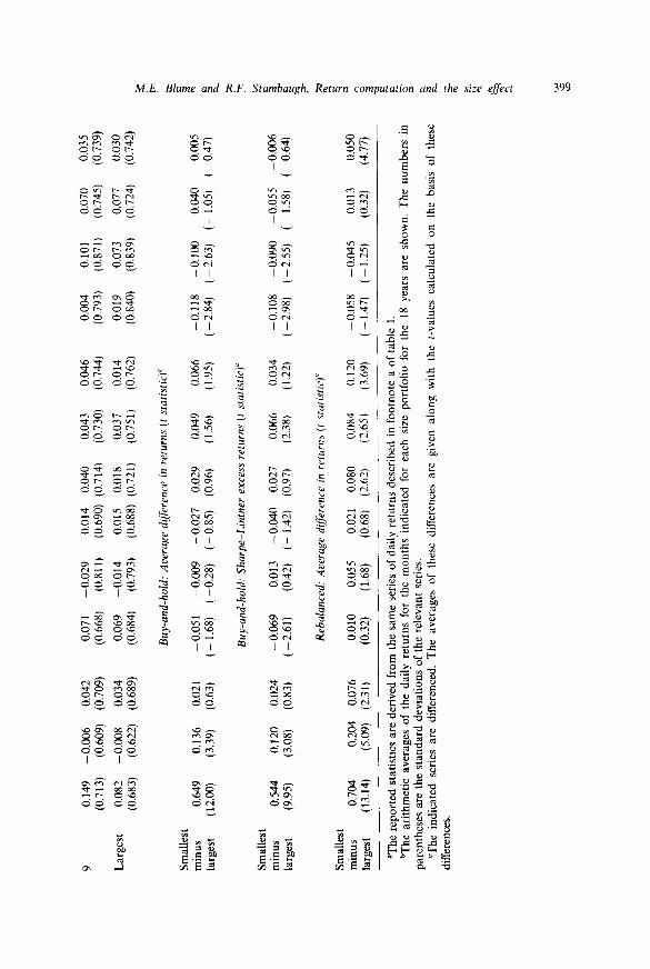
of the average size effect can be attributed to the month of January. The average daily returns for rebalanced portfolios shown in table 2 are consistent with Keim's analysis. In contrast, inferences about the size effect based upon buy-and-hold returns differ markedly from those of Keim. On average over the 1963 80 period, there is a strong January size effect. However, on average over the eleven remaining months, there is no pronounced size effect. 18 Over these months, the average return on the smallest firms minus the average return on the largest firms is -0 .005 percent per day with a t statistic of -0.47. In fact, of the ten portfolios from February through December, the smallest-firm portfolio actually has one of the l~west average daily returns.
In addition, the reader should note that for each of the twelve months, the average measure of the size effect as computed with rebalanced returns exceeds the average measure as computed with the buy-and-hold returns by about 0.05 percent per day. This relatively constant difference is to be expected if the bid-ask phenomenon is stationary across months.
A closer examination of the month-by-month buy-and-hold returns from February through December reveals some size effects that, depending on the month, go in either direction. Yet, even the largest numbers in absolute value for the last eleven months are small in comparison to those of January: for example, February's value is about one-fifth of January's.
On average over these eighteen years, there seems to be little evidence of any consistent size effect in the last eleven months of the year. Indeed, the full-year average size effect of 0.051 percent is roughly 1/12 of the January value of 0.649 percent. Nonetheless, an examination of the data by subperiods discloses some non-stationary size effects in the last eleven months of the year. For the last eleven months, the size effect is 0.096 percent for 1963 68, 0.113 percent for 1969 74, and 0.0041 percent for 1975 80 with respective t-values of 6.45, -6.13, and 0.20. For comparison, the January effect varies less across these three subperiods relative to its magnitude from 0.429 percent for 1963-68 to 0.815 percent for 1975 80 with a minimum t-value of 6.40.
3.3. Adjustments.]br risk
The portfolio returns discussed above are not adjusted for risk, as previous studies, such as Reinganum (1981b, 1982), find that various methods of risk adjustment do little to change inferences about the size effect. Nevertheless, some analysis of risk-adjusted returns is certainly warranted.
A common criterion for adjusting for risk is to define excess returns as
'sWe investigated whether the seasonality is sensitive to the time of the initial porlfolio formation. The same year-end rankings were used to form buy-and-hold portfolios with equal weights at the beginning of the subsequent July with virtually identical resuhs.

M.E. Blume and R.F. Stambaugh, Return computation and the size effect 401
those that violate the implications of the Sharpe-Lintner version of the two- parameter model. To implement this criterion, define Rs, as the return on the small-firm portfolio, RLt as the large-firm return, RMt as the return on the market portfolio, and Rvt as the riskless interest rate. Consider the regression equation
(Rs, - RLt) = a + fl(RMt -- Rvt) + e,~, (lS)
where et is an independent disturbance with zero expectation. The Sharpe Lintner model implies that a=0 . A non-zero value of a is interpreted as the excess return of small firms relative to large firms or, alternatively, the risk- adjusted size effect.
Roll (1981) suggests that infrequent trading is more often associated with small firms, and, if so, ordinary least-squares estimates of betas for these firms using daily data may be downward biased. The aggregated coefficient method of Dimson (1979) is used to adjust for this effect by estimating the regression
5
( R s t - R L t ) = c ~ + ~ flk(RM,,+k--R~.~+k)+e ,, (16) k - 15
where R M is the daily return on the S&P 500 index and R v is the daily return on a one-month T-bill (held constant within a given calendar month). The estimates of ~ and their t statistics are reported as 'Sharpe-Lintner excess returns' in table 2. The magnitude of the size effect is reduced slightly, but the changes are too small to alter any of the previous discussion.
4. A further investigation of the bias
Demsetz (1968) and more recently Branch and Freed (1977) postulate and find that the bid-ask spread of an individual stock as a percentage of its price is negatively and strongly related to the price of the stock itself in models that hold other possible explanatory variables constant. Since the bias due to the bid-ask effect is related to the variance of the percentage bid- ask spread, it seems natural to examine the relation between price and this bias. As a rough attempt to hold other variables constant, the subsequent analysis of price will control for differences in market value.
For each year, the stocks in each market value decile are partitioned into subgroups according to the closing price of the prior year. The price classifications are $2 or less, $2 to less than $5, $5 to less than $10, and $15 to less than $20. Stocks with closing prices of $20 or more are dropped since the two studies cited above suggest that the strong relation of percentage bid-ask spread to price is due primarily to lower-priced stocks.

402 ),t.t:'. Blume aml R.F. Stamhaugh, Return computation and the size g[fi'et
The expected difference between the calculated average daily rebalanced and buy-and-hold return is a function of the number of securities in the portfolio and increases as the number of securities increases. With 10 or more securities, an examination of (14) shows that the expected differences in the calculated returns do not change rapidly with the number of securities. For example, the expected difference in calculated returns for a portfolio of 100 securities, all with the same statistical properties, is only 10"Jo greater than for a portfolio of 10 of these securities. Thus, to avoid having to consider explicitly the number of securities in each portfolio, the following analysis uses only portfolios of l0 or more securities.
The average daily differences between the rebalanced and buy-and-hold returns, shown in table 3, exhibit a strong negative relation to price, when market value is held constant, but little, if any, relation to market value, once price is held constant. For instance, for the second-smallest market value group, the average difference between the computed daily returns for the rebalanced and buy-and-hold portfolios is 0.136!'~,, for the 0 to $2 range but only 0.00083; for the $15 to $20 price range. Similar negative relations appear in every market value category for which data are available.
The monotonic relationships observed in table 3 are strong. For example, there is virtually no overlap in the differences between the rebalanced and buy-and-hold portfolios as between the lowest price category ($(>$2) and the next price category ($2-$5). Of the 61 observations in the second lowest price category, 58 of the differences are less than the smallest difference in the lowest price group. Even the largest difference in the second lowest price group exceeds only 4 of the 26 observations in the lowest price group.
The significance of the relations suggested by table 3 is tested as follows. First, for each year, the average daily differences between the rebalanced and buy-and-hold returns are computed for each portfolio cross-classified by price and market value. Second, these average differences are regressed upon a constant, four dummy variables for price classes, and nine dummy variables for market value classes, t9 Because the dependent variables in this regression are differences between computed returns of portfolios of the same securities, there is no reason to believe that there will be any substantial contemporaneous correlation in the residuals. Indeed, an analysis of the residuals themselves finds little contemporaneous correlation.
The k' statistic that tests whether the coefficients on the price dummy variables are jointly zero is 394.84 with 4 and 397 degrees of freedom, which
l 'qn order to focus on cross-sectional effects, the intercept in the regression is allowed to wiry from year to year through the inclusion of seventeen dummy variables for time. The F statistic for the coefficients on the dummies for time is 7.89 with 17 and 397 degrees of freedom, which is significant at the one percent level. Although not related to the measurement of cross-sectional effects but perhaps of interest for some subsequent research, the coefficients on the time dummy variables do not appear to be measuring a simple trend: the correlation between time itself and the time dummy variable coefficients is 0.028.

M.E. Blume and R.F. Stambaugh, Return computation and the size effect 403
Table 3 Average daily percent returns for rebalanced minus buy-and-hold portfolios cross-classified by market values and stock prices, 1963-1980 (number of years of available data shown in
parentheses)2
Market value decile
Price range 1 2 3 4 5 6 7 8 9 10
$0 to 0.1412 0.1360 0.1425 0.1287 0.0987 less than $2 (13) (8) (3) (1) (1)
$2 to 0.0378 0.0454 0.0458 0.0416 0.0391 0.0373 0.0289 0.0444 less than $5 (17) (15) (9) (8) (6) (3) (2) (1)
$5to 0.0182 0.0195 0.0150 0.0149 0.0106 0.0059 0.0119 0.0170 0.0157 less than $10 (15) (17) (16) (17) (11) (8) (8) (41 (2)
$10 to 0.0075 0.0099 0.0064 0.0073 0.0075 0.0078 0.0048 0.0060 0.0078 0.0060 less than $15 (11) (15) (16) (17) (15) (15) (11) (8) (7) (4)
$15to 0.0027 0.0008 0.0030 0.0043 0.0057 0.0027 0.0041 0.0056 0.0064 0.0038 less than $20 (3) (12) (15) (16) (16) (17) (15) (13) (10) (7)
"For each year, portfolios are formed by market value at the end of the prior year. Each of these portfolios is then partitioned according to the stock price at the end of the prior year; at this stage, any stock with a stock price of $20 or more is discarded for reasons discussed in the text. For each year for which there is a marl~et value price portfolio with 10 or more securities, the difference between the average daily rebalanced and buy-and-hold returns is calculated. The averages of these differences are reported in this table along with the number of years of available data.
is significant at any usual level. The corresponding F statistic for the coefficients on the dummies for market value is 0.34 with 9 and 397 degrees of freedom, which is not significant at any usual level.
In sum, the differences between rebalanced and buy-and-hold average daily returns are significantly related to price and weakly, if at all, to market value. The strong negative relation to price is consistent with the 'bid-ask' phenomenon, but it does not preclude other explanations.
5. Conclusions
Individual stock returns computed with closing prices are upward biased, primarily due to a 'bid ask' effect. The computed return on a rebalanced portfolio is also upward biased, since such a return is simply an arithmetic average of returns on individual stocks. The computed return on a buy-and- hold portfolio largely avoids the bid-ask bias due to a 'diversification' effect. The size of the bias in daily returns on stocks of small firms is sufficient to alter substantially conclusions about the size effect. Based on buy-and-hold daily returns, the full-year size effect is half as large as previously reported using rebalanced returns, and, on average, all of the size effect is due to the month of January.

404 M.E. Blume and R.b. Stambau~,,h. Return computation and the size ~JJg'ct
T h e i m p l i c a t i o n s of this s t u d y reach b e y o n d c o n s i d e r a t i o n of the size effect.
T h e biases a n a l y z e d here , w h i c h are s o m e t i m e s subs t an t i a l , can p o t e n t i a l l y
ar ise in a n y s t u d y t h a t f o r m s e q u a l l y - w e i g h t e d r e b a l a n c e d po r t fo l io s (or,
m o r e genera l ly , a n y po r t fo l i o wi th we igh t s tha t are u n c o r r e l a t e d wi th
c o m p u t e d re turns) . T h e s e b iases can be g rea t ly r e d u c e d by us ing r e t u r n s
impl ic i t in a b u y - a n d - h o l d s t ra tegy .
References
Banz. R.W., 1981, The relationship between return and market value of common stocks, Journal of Financial Economics 9, 3 18.
Blume, M.E. and I. Friend, 1974, Risk, investment strategy, and the long-run rates of return, Review of Economics and Statistics 56, 259 269.
Branch, B. and W. Freed, 1977, Bid asked spreads on the AMEX and the Big Board, Journal of Finance 32, 159 163.
Brown. P., A.W. Kleidon and T.A. Marsh. 1983. New evidence on the nature of size related anomalies in stock prices, Journal of Financial Economics 12, 33 56.
Cheng, P i . and M.K. Deets, 1971, Portfolio returns and the random walk theory, Journal of Finance 26, 11 30.
Demsetz, H., 1968, The cost of transacting, Quarterly Journal of Economics 82, 33 53. Dimson, E., 1979, Risk measurement when shares are subject to infrequent trading, Journal of
Financial Economics 7, 197 226. Fisher, L., 1966, Some new stock market indices, Journal of Business 29, 191 225. Keim, D.B., 1983, Size related anomalies and stock return seasonality: Eurlher empirical
evidence, Journal of Financial Economics 12, 13 32. Niederhoffer. V. and M.F.M. Osborne, 1966, Market making and reversal on the Stock
Exchange, Journal of the American Stalistical Association 61. 897 916. Reinganum, M.R., 1981a, Misspecification of capital asset pricing: Empirical anomalics bascd ~m
earnings' yields and market values, Journal of Financial Economics 9, 19 46. Reinganum, M.R., 1981b, The arbitrage pricing theory: Some empirical results, Journal of
t:inance 36, 313-321. Rcinganurn, M.R., 1982, A direct test of Roll's conjecture on the firm size effect, Journal of
Finance 37, 27 35. Reinganum, M.R.. 1983, The anomalous stock market behavior of small firms m Jalluary:
Empirical tests for tax-loss selling effects, Journal of Financial Economics 12, 89 104. Roll, R., 1981, A possible explanation of the small firm effect, ,lournal of Finance 36, 879 888. Roll, R., 1983, On computing mean returns and the small firm premium, Journal of Financial
[-conomics, this issue. Scholes, M. and J. Williams, 1977, Estimating betas from non-synchronous data, Journal of
I.'inancial Economics 5, 309 327. Stock quotations on the New York Stock Exchange, 1973 1Francis Emory l:itch, New York). Sloll, H.R. and R.E. Whalcy, 1983, Transaction costs and Ihe small firm efli:ct. Journal of
Financial Economics 12. 57 79.