bias adjustment of satellite rainfall data through...
TRANSCRIPT

Bias adjustment of satellite rainfall data through stochastic
modeling: Methods development and application to Nepal
Marc F. Muller∗, Sally E. Thompson
Department of Civil and Environmental Engineering, Davis Hall, University of California, BerkeleyCA, USA
Abstract
Estimating precipitation over large spatial areas remains a challenging problem forhydrologists. Sparse ground-based gauge networks do not provide a robust basis forinterpolation, and the reliability of remote sensing products, although improving, isstill imperfect. Current techniques to estimate precipitation rely on combining thesedifferent kinds of measurements to correct the bias in the satellite observations. Wepropose a novel procedure that, unlike existing techniques, (i) allows correcting thepossibly confounding effects of different sources of errors in satellite estimates, (ii)explicitly accounts for the spatial heterogeneity of the biases and (iii) allows the useof non overlapping historical observations. The proposed method spatially aggregatesand interpolates gauge data at the satellite grid resolution by focusing on parametersthat describe the frequency and intensity of the rainfall observed at the gauges. Theresulting gridded parameters can then be used to adjust the probability density functionof satellite rainfall observations at each grid cell, accounting for spatial heterogeneity.Unlike alternate methods, we explicitly adjust biases on rainfall frequency in additionto its intensity. Adjusted rainfall distributions can then readily be applied as input instochastic rainfall generators or frequency domain hydrological models. Finally, we alsoprovide a procedure to use them to correct remotely sensed rainfall time series.
We apply the method to adjust the distributions of daily rainfall observed by theTRMM satellite in Nepal, which exemplifies the challenges associated with a sparsegauge network and large biases due to complex topography. In a cross-validation anal-ysis on daily rainfall from TRMM 3B42 v6, we find that using a small subset of theavailable gauges, the proposed method outperforms local rainfall estimations using thecomplete network of available gauges to directly interpolate local rainfall or correctTRMM by adjusting monthly means. We conclude that the proposed frequency-domainbias correction approach is robust and reliable compared to other bias correction ap-
∗Corresponding authorEmail addresses: [email protected] (Marc F. Muller),
[email protected] (Sally E. Thompson)
Preprint submitted to Advances in Water Resources Saturday 27th July, 2013

proaches.
Keywords: Bias Correction, Remote Sensing, Stochastic Model, Areal Precipitation,Rainfall Interpolation, Himalayas
1. Introduction
Spatially explicit rainfall estimates are crucial for hydrologic predictions, but due tochallenges in observing rainfall at watershed scales, rainfall estimates remain a majorsource of uncertainty for hydrologic models (1). In many parts of the world, ground-based rain-gauge networks are irregular and locally sparse (2), and may be biased withrespect to the sources of environmental variability (see Figure 1 for an example). Suchnetworks do not provide a robust basis for inferring the spatial pattern of rainfall fields.An alternative and explicitly spatial rainfall product is provided by satellite obser-vations of precipitation. Unfortunately, satellite observations of rainfall have widelyacknowledged limitations, including sensitivity to precipitation type (3), underestima-tion of orographic rainfall (4), a tendency to miss snowfall (5), inability to captureshort rainfall events (6) and systematic biases in mountainous areas (7, 8, 5, 9). Usingground-based data to correct biases in satellite data provides one method to addressthese limitations. For example, the satellite observations in the NASA Tropical RainfallMeasuring Mission (TRMM) 3B42 dataset are adjusted using monthly-averaged groundobservations provided by local monitoring agencies to the Global Precipitation Clima-tology Centre (GPCC) (3). However, the efficiency of the adjustment is limited by thescarcity of available gauges and typically requires careful regional evaluation againstlocal precipitation measurements.
The correction applied by NASA on TRMM is a standard bias adjustment procedurefor satellite rainfall observations, based on correcting rainfall time series - in this caseby regression analysis applied to cumulative rainfall totals (7, 10, 11). Other standardprocedures adjust quantiles of the daily rainfall to match those observed at gauges (12).These approaches suffer from several drawbacks:
1. Biases in TRMM observations of rainfall timeseries are influenced by errors inboth rainfall frequency and rainfall intensity, which may have opposite signs (13).Adjusting satellite precipitation totals or PDFs will thus correct errors in themagnitude of rainfall, but not in its temporal structure, although both factors areimportant for hydrological predictions (14, 15).
2. Although some recent studies account for the observed spatial heterogeneity inbiases, and in doing so significantly improved the corrected dataset (10, 11), ap-proaches based on preserving regional rainfall totals often do not account forspatial patterns in bias or focus on single precipitation stations. One of the fac-tors that makes spatially-explicit corrections challenging is the upscaling of pointobservations from gauges to areal rainfall at the resolution of the satellite grid.
2
3. Finally, correction of monthly time series on a pixel by pixel basis is numeri-cally intensive, and cannot take advantage of historical rainfall datasets which,although not overlapping with contemporary observations, may still contain usefulinformation about spatial patterns in rainfall.
We therefore propose an alternative strategy for bias adjustment of satellite rainfalldata using ground-based gauge observations. Instead of adjusting daily rainfall tomatch the mean monthly precipitation, we perform the bias adjustment on a set of(pseudo)stationary stochastic parameters that describe the rainfall process in terms offrequency, intensity, and the autocorrelation of wet and dry periods (16, 17, 18). Thisapproach addresses the key limitations of time series based bias adjustment:
1. It is a direct response to the observation of different directionality in TRMM-gaugebias arising due to different and independent features of the rainfall time series(13). This observation implies that separating the bias adjustment for rainfalloccurrence and intensity might improve the robustness of the resulting rainfallestimates.
2. It allows different features of rainfall to be independently interpolated accountingfor spatial heterogeneity and, unlike existing studies, also accounting for potentialdifferences in spatial heterogeneities between stochastic rainfall features.
3. Being in the frequency domain, the bias adjustment can be operated using nonoverlapping observed time series provided stationarity conditions are satisfied.
A key contribution of the proposed procedure lies in its ability to spatially aggregateand interpolate the stochastic rainfall descriptors at the grid resolution. This provides aground truth estimate of the daily rainfall distribution at each pixel that can be used tocorrect satellite rainfall distributions, with two potential applications. Firstly, grid-scalerainfall cumulative probability densities are valuable for correcting rainfall timeseriesmagnitudes via quantile mapping (12). Our proposed method explores the upscalingof gauge-derived rainfall PDFs and their spatial interpolation, allowing corrections tothe rainfall CDF to be applied in a spatially explicit fashion. Moreover, the procedureupscales and interpolates information about the autocorrelation of rainfall, allowingthe bias adjustment procedure to correct the temporal structure of satellite rainfallobservations as well as the magnitudes. Since the temporal structure of rainfall isan important driver of hydrological responses in the vadose zone (14) and in the flowregime (15), incorporating this information into satellite bias correction is a usefuladvance. The stochastic parameters may be directly utilized in stochastic descriptionof the resulting streamflow (15); used to generate ensembles of synthetic time series datausing stochastic weather generation models (19, 20), or incorporated into time-seriescorrection approaches (as outlined in Section 2.5).
The proposed approaches are illustrated here using Nepal as a case study. Nepalprovides an excellent opportunity to test the new bias correction procedure because twosatellite rainfall products are available that incorporate very different bias-adjustmenttechniques: TRMMv6 and TRMMv7. The major distinction between the two datasets
3
for terrestrial rainfall estimates lies in the rain gauge datasets used for monthly biasadjustment (21). In Nepal the number of considered gauges increases from 11 (GPCCmonitoring dataset v2) to 280 gauges (GPCC full analysis dataset v6). Thus, TRMMv6in Nepal represents a satellite rainfall data product with minimal ground-based correc-tion, while TRMM v7 represents satellite data corrected using conventional time seriesadjustment. In this study, we therefore develop a bias adjustment technique, applyit to TRMM v6 and compare the results against the performance of TRMM v7 as abenchmark.
We first describe a stochastic rainfall model (Section 2.1) and its use to adjustsatellite rainfall observation biases through space. Spatial adjustment of stochastic pa-rameters is not straightforward because of their nonlinear relationships to the momentsand time-structure of the rainfall distribution. To estimate bias, the stochastic modelparameters obtained from point-scale rainfall measurements at gauges are spatially ag-gregated to the scale of a satellite observation pixel (Section 2.2). The stochastic modelparameters estimated at the pixel scale are then spatially interpolated to provide es-timates at the satellite pixels devoid of gauges (Section 2.3). Section 2.4 summarizesthe method to correct the bias of gridded, remotely sensed daily rainfall observationsin the frequency domain using multi-site gauge observations – the main contributionof this paper. Using bias adjusted frequency domain information, rainfall time seriescan then easily be adjusted through quantile mapping (Section 2.5). An illustrativeexample of time series correction is given in Section 3.2.6. The remainder of the paperfocuses on assessing the performance of the frequency domain bias correction method,which underpins both the stochastic and time-series adjustments. The sensitivity ofthe method to common sources of uncertainties is first assessed in a Monte Carlo anal-ysis (Sections 3.1), and its ability to adjust the frequency, mean intensity and varianceof actual remote sensing rainfall data is assessed in a cross validation analysis usingNepalese rainfall for various densities of gauge networks (Section 3.2). The main resultsand their implications are discussed in Section 4 and Section 5 concludes.
2. Theory
2.1. Stochastic Model
We use a two-step stochastic weather generator to represent the statistical propertiesof the rainfall time series. We firstly disaggregate the time series into two independentseasons (16) – the dry season and the monsoon. We identify the seasons by the calen-dar days corresponding to the average start date (RnStr) and end date (RnStp) of themonsoon. Next, we describe the rainfall for each season in terms of two stochastic pro-cesses: the daily occurrence, and daily intensity of rainfall. We use a first-order Markovchain model to represent rainfall occurrence (17, 18). This model is governed by twoparameters P01 and P11, which characterize the probability of a rainy day, conditionalon the previous day being dry (P01) or rainy (P11). We use a gamma distribution with
4

shape parameter GS and rate parameter GR to describe the probability distribution ofdaily rainfall depths on those days when rain occurred. This representation of rainfallrequires a total of 10 stochastic model parameters (SMPs) listed in Table 2. These modelparameters are directly related to a range of relevant metrics that describe rainfall dis-tribution and can thus be used to evaluate the bias adjustment method. These metricsare derived in Appendix A and include the length of wet and dry spells, the number ofrainy days per year, the unconditional variance on daily rainfall and the average annualrainfall .
2.2. Areal Aggregation of Stochastic Model Parameters
While gauges monitor precipitation at particular points, satellites observe an areallyaveraged value of rainfall over many square kilometers. Correcting remote sensing pre-cipitation observations therefore requires spatially aggregating point-scale precipitationparameters to the level of the satellite resolution. We perform this aggregation analyt-ically, rather than directly from the time series because (i) it is more computationallyefficient and (ii) it allows us to use data provided by on (stationary) rainfall gaugesthat do not overlap in time with the TRMM observation window. We outline the ap-plicability of the methods to the case study with TRMM in Nepal below, including anevaluation of the stationarity of ground-based rainfall measurements in terms of the 10SMPs.
2.2.1. Seasonal Parameters
We assume that the starting day of the rainy and dry seasons at the pixel level canbe approximated by the weighted average of the corresponding values across the Np
gauges in the pixel,
Strpix =
Np∑i=1
aiStri Str ∈ {RnStr,RnStp} (1)
where ai is the proportion of the pixel’s area covered by a Thiessen polygon centeredon gauge i.
2.2.2. Occurrence Parameters
A pixel should be classified as ‘rainy’ on a given day if rain occurs at any of itsgauges during that day. Thus the probability of rain at the level of a pixel is nota simple average of the occurrence probabilities at the gauges within the pixel, but ismodified by the correlation between the gauges. If the correlation length-scale of rainfallexceeds the pixel size, then it is reasonable to assume that the correlation between therain occurrence probabilities Pi at the different gauges is positive and maximal. That is,if the gauge that is most likely to receive rainfall is dry, the pixel is also dry. Using this
5

assumption, the probability of rainfall in a pixel is well approximated by the maximumoccurrence probability across the Np gauges within that pixel, as:
Ppix ≈ maxPi (2)
A similar assumption about the ratio of wet-to-wet transitions Pi · P11,i leads to thefollowing estimate for the pixel-level transition probability:
P11,pix ≈ max
{max (Pi · P11,i)
Ppix; 1−
∑Ni=1 Pi · (1− P11,i)
Ppix
}(3)
where the transition probability P11 at the satellite pixel level can be approximated byits lower bound. This bound is given by the higher of (i) the maximal value of wet-to-wet ratio (P · P11) and (ii) the sum of wet-to-dry transition ratios (P · P10) withinthat pixel. The full derivation of equations 2 and 3 is presented in Appendix B. Ourcase study in Nepal is characterized by a maximum density of 5 gauges per pixel andspatial autocorrelation ranges of approximately 3 (dry season) to 4 (wet season) timesthe pixel size of 27.7km (Table 4), meeting the assumptions used in the derivation ofequations 2 and 3. We tested the performance of the aggregation equations via a MonteCarlo analysis. We found that using equations 2 and 3 generated less than 2% error inboth metrics (Pi and Pi · P11,i). This error declined with an increase in the correlationlength scale, but increased with increasing numbers of gauges per pixel.
2.2.3. Intensity Parameters
To aggregate rainfall intensity we preserve the weighted average of the first twomoments of the distributions measured at each gauge, using the Thiessen polygon arearatios ai as weights. Doing so based on the SMPs that describe the rainfall intensity(GS and GR) poses three challenges. Firstly, the SMPs are non linearly related to themoments of the gamma distribution:
E [X | wet] = GS/GR (4)
Var (X | wet) = GS/GR2. (5)
Thus, aggregating the weighted sum of the distribution’s parameters is not equivalentto aggregating the distribution’s moments. Secondly, the parameters represent thedistribution of rainfall intensity conditional on rainfall occurrence, so the probability Pof rainfall occurrence must be incorporated into the aggregation. Finally, the varianceof areal rainfall is affected by spatial autocorrelation. A full derivation of the upscalingrelationship for the rainfall intensity properties, accounting for these three challenges, isprovided in Appendix C. The methodology used consists of (i) conditioning for rainfalloccurrence and the location of individual gauges, (ii) applying the laws of iteratedexpectation and total variance to compute the mean and variance of rainfall intensity
6

at the pixel scale (Equations 6 and 7) and (iii) correcting the variance of areal rainfallto account for the transition from point to areal probabilities (22). We assume thesame functional form of the PDF applies to pixels and all gauges, meaning that thepixel-scale rainfall intensity is a gamma distribution and that its parameters GS andGR are directly related to its mean and variance as in Equations 4 and 5. With theseassumptions, we obtain the expectation and variance of the pixel-level areal rainfall as:
E [Xpix | wet] =1
Ppix·
N∑i=1
aiPiE [Xi|wet] (6)
Var (Xpix | wet) =
=C(d)
Ppix
[N∑i=1
aiPi
(Var (Xi | wet) + PiE [Xi | wet]2 − PiE [Xi | wet]
)]+ C(d)Ppix
[E [Xpix | wet]− E [Xpix | wet]2
], (7)
where Pi is the probability of rainfall occurrence at the gauge level, and Ppix is theprobability of rainfall occurrence at the pixel level (from Equation 2). C(d) is anattenuation factor applied to the variance of areal rainfall based on the derivation ofRodriguez-Iturbe and Mejıa (22):
C(d) =
∫ √2dr(ν)f(ν)dν ≤ 1,
where r(ν) is the spatial correlation function of rainfall intensity and f(ν) is the dis-tribution of distances between two points chosen at random in the pixel. Point-scalerainfall typically over-estimates the variance of areal rainfall, so C(d) < 1. C(d) in-creases with pixel size d and decreases with the spatial autocorrelation range, both ofwhich are typically spatially homogenous. In Nepal we estimated C(27.7km) as 0.75 inthe monsoon and 0.86 in the dry season, using a correlogram estimated from the spatialdistribution of rainfall intensity at gauges over 2,000 randomly selected days.
2.3. Spatial Interpolation of Stochastic Model Parameters
A typical spatial interpolation methodology would approximate daily rainfall X atunmonitored locations as linear combinations of Xi the rainfall measured at surroundinglocations i on the same day, weighted by vXi , a normalized similarity metric based onrelative position (e.g. inverse weighted distance) or the spatial correlation function ofX (e.g. kriging):
X =
Ng∑i=1
v(X)i Xi (8)
7

Interpolation of the probabilistic descriptors of the rainfall, however, cannot be under-taken by directly interpolating the SMP’s because neither the moments of the gammadistribution of conditional rainfall intensity nor the moments of the binomial distri-bution of daily rainfall occurrence are linear combinations of the SMPs. Thus, weinterpolate the moments of the distributions, expressed as functions of the SMPs. Weassume that interpolation must preserve seasonal transition dates (RnStr and RnStp),the daily occurrence probability of rainfall (P ) and the ratio of wet-to-wet transitions(P · P11). This allows us to express the interpolated rainfall metrics as linear combina-tions of their respective values at the Ng observed locations, which are directly relatedto the observed SMPs:
Str =
Ng∑i=1
v(Str)i Stri Str ∈ {RnStr,RnStp} (9)
P =
Ng∑i=1
v(P )i Pi =
Ng∑i=1
v(P )i
P01,i
1 + P01,i − P11,i
(10)
P · P11 =
Ng∑i=1
v(P ·P11)i Pi · P11,i =
Ng∑i=1
v(P ·P11)i
P11,iP01,i
1 + P01,i − P11,i
(11)
Using similar reasoning to that in section 2.2, but replacing area weights ai withinterpolation weights v
(E)i , we compute the interpolated moments of the distribution
of conditional rainfall intensity. Here we use weights v(E)i generated from kriging of
the expected rainfall E [Xi] for the interpolation of both the mean and variance of therainfall PDF. Either ordinary kriging or univerval kriging can be used (23, 24). For thisinterpolation, we do not use the attenuation factor C(d) as there is no point to areatransformation. From equations 6 and 7 we obtain the expectation and variance of therainfall at the ungauged location:
E[X | wet
]=
1
P·
Ng∑i=1
v(E)i PiE [Xi|wet] (12)
Var(X | wet
)=
=1
P
[Ng∑i=1
v(E)i Pi
(Var (Xi | wet) + PiE [Xi | wet]2 − PiE [Xi | wet]
)]
+ P
[E[X | wet
]− E
[X | wet
]2](13)
where Pi is the probability of rainfall occurrence at the observation point i, and P theinterpolated probability of rainfall given by Equation 10.
8

2.4. Bias adjustment of Stochastic Model Parameters
The bias adjustment approach is based on the assumption of spatial correlation inthe differences in daily rainfall between the TRMM pixels and the (aggregated) gauges.Biases at pixels devoid of gauges can then be estimated by interpolating the biasesobserved at pixels that contain gauges. Interpolating the biases for each stochasticparameter to un-gauged pixels raises the same problems as interpolating the stochasticparameters within the pixels (Section 2.3). Thus, we independently interpolate theSMPs estimated from TRMMv6 at gauged pixels and the pixel-scale SMPs estimatedfrom the gauges (and not the difference between them), before computing the biasesat ungauged pixels as the difference between the two interpolations. The full biasadjustment procedure thus consists of the following steps:
(i) Aggregating the SMPs observed at the gauges to the resolution of TRMM pixels(Section 2.2).
(ii) Interpolating the aggregated SMPs from the gauged to the ungauged pixels (Sec-tion 2.3), labeled as ˜SMPpix .
(iii) Interpolating the SMPs obtained for TRMMv6 at the gauged pixels to the un-gauged pixels (Section 2.3), labeled as ˜SMPTRMM.
(iv) Computing the biases ˜∆SMPTRMM at ungauged pixels by subtracting the resultof step (ii) ( ˜SMPpix) to the result of step (iii) ( ˜SMPTRMM).
(v) Finally, biases are adjusted by subtracting the modeled bias ˜∆SMPTRMM fromSMPTRMM, the local SMPs of TRMMv6:
SMPadjusted = SMPTRMM − ˜∆SMPTRMM = SMPTRMM −(
˜SMPTRMM − ˜SMPpix
).
Assuming rainfall follows the stochastic model described in section 2.1, this procedureallows the bias adjusted distribution of rainfall to be estimated for all pixels.
2.5. Bias adjustment of time series
A useful application of the bias adjusted distribution of rainfall obtained in the pre-vious section is its use to correct remotely sensed time series through quantile mapping.Quantile mapping is a well established technique (see (12) for a review) that, in the
context of this paper, attempts to find a transformation of X(t)TRMM , the remotely sensed
rainfall observation at time t, such that its new distribution equals the distribution ofX
(t)adj, the corresponding bias adjusted rainfall observation. The distribution of X
(t)TRMM
can be readily characterized from remote sensing observations. The method presentedin Section 2.2.3 provides the bias corrected distribution of rainfall (i.e the distribution
of X(t)adj). The transformation can therefore be written as
X(t)adj = F−1adj (FTRMM(X
(t)TRMM)) (14)
where F−1adj (·) is the inverse of the bias adjusted cumulative distribution function andFTRMM(·) is the cumulative distribution function of remotely sensed rainfall at the con-
9

sidered pixel. FTRMM(X(t)) can be calculated using the relevant stochastic model param-eters obtained from remotely sensed rainfall by applying the law of total probabilities:
FTRMM(X(t)TRMM) = (1− PTRMM) + PTRMM · FTRMM,w(X
(t)TRMM) (15)
where PTRMM = P01,TRMM if X(t−1)TRMM = 0 and PTRMM = P11,TRMM otherwise; and where
FTRMM,w(X(t)) is the cumulative distribution function of a gamma distribution with rateGRTRMM and shape GSTRMM. Similarly, the bias-adjusted cdf Fadj can be calculatedusing the bias-adjusted stochastic model parameters.
Fadj(X(t)adj) = (1− Padj) + Padj · Fadj,w(X
(t)adj) (16)
where Padj = P01,adj if X(t−1)adj = 0 and Padj = P11,adj otherwise; and where Fadj,w(Y (t)) is
the cumulative distribution function of a gamma distribution with rate GRadj and shapeGSadj. We define the inverse of Fadj(·) as
F−1adj (Y(t)) =
{0 if Y (t) ≤ 1− Padj
F−1adj,w(Y (t)) otherwise(17)
Note that FTRMM(·) has a discontinuity at zero. Therefore, its image doesn’t spanall possible probabilities between zero and one (i.e. values below PTRMM are excludedfrom the image). When applying quantile mapping (Equation 14) part of the rainfall
range is therefore censored. For example if Fadj(0) < 1 − PTRMM, all values of X(t)TRMM
will be mapped to positive rainfall.1 In other words, a dry data point in TRMMis always matched to the largest rainfall value X
(t)adj that occurs with the probability
FTRMM(0) in our model. Of course, any rainfall prediction below this cutoff would bejust as reasonable. To avoid artificial overestimation of rainfall occurrence, we thereforematch a dry TRMM data point to a random sample from the conditional distributionFadj(x | x ≤ X
(t)adj), given by
Fadj(x | x ≤ X(t)adj) =
Fadj(x)
Fadj(X(t)adj )
if x ∈ [0, X(t)adj]
1 if x > X(t)adj.
(18)
This correction ensures that we preserve the actual rainfall distribution (including rain-fall occurrence) for large samples.
To summarize, we first determine which stochastic model parameters to use accord-ing to the season of X
(t)TRMM (Monsoon vs. dry season) and the rainfall occurrence
1One particular concern is artificial oscillation of rainfall occurrence during dry periods, whenPadj,01 < PTRMM < Padj,11 (or Padj,11 < PTRMM < Padj,01).
10

status at X(t−1)TRMM (wet vs. dry). Then,
• if X(t)TRMM > 0, we apply Equation 15 to get the probability of X
(t)TRMM , on which
we finally apply Equation 17 to get the corresponding quantile in the adjustedrainfall distribution.• if X
(t)TRMM = 0 we have FTRMM(X
(t)TRMM) = PTRMM and are confronted to the
discontinuity problem mentioned above. The case where F−1adj (PTRMM) = 0 results
in a dry day and X(t)adj = 0. If F−1adj (PTRMM) > 0, X
(t)adj is stochastically determined as
a random draw from the distribution, which cdf is described in Equation 18. Thisis equivalent to the practically more convenient option of a random draw fromthe distribution in Equation 16 with rejection of samples above F−1adj (PTRMM).
3. Methods
The methods section describes the metrics used to evaluate the bias adjustmentprocess of stochastic model parameters described in section 2.4, and a Monte Carloanalysis in which the performance of the process was tested on synthetic data (Section3.1). It then outlines the application of the technique to rainfall data in Nepal (Section3.2). As part of this application we characterize the bias in TRMM observations (Sec-tion 3.2.3), and perform a jack-knife cross validation (25) to assess the performance ofthe bias-adjustment technique (Section 3.2.5). Finally, an example of the applicationof the adjusted stochastic model parameters to correct TRMM time series is given inSection 3.2.6. The stochastic model, bias adjustment methods and time series correc-tion procedure were compiled in an R script (26) and are provided as supplementarymaterial.
3.1. Monte Carlo Analysis
To evaluate the performance of the bias adjustment we focus on the mean absoluteerrors (MAE) in annual rainfall. The MAE avoids outlier compensation effects, wherebyoverestimation at one gauge may cancel out the underestimation at another (leadingto under-estimation of the true error). The MAE of annual rainfall provides a scalarperformance metric that combines errors in the occurrence, intensity and seasonalityof rainfall and is easily understood in physical terms. We also compute MAEs for thevariance and occurrence probability of daily rainfall.
We run a Monte Carlo analysis using synthetic data to evaluate the properties ofour bias adjustment technique and its sensitivity to a range of characteristics of thegauge network and TRMM observations (presented in Table 3).
We apply the following procedure to generate a synthetic rainfall surface, TRMMdata and gauge observations that are representative of our case study site (Nepal):
1. The SMP values observed at Nepalese gauges are interpolated by ordinary krigingonto a 0.05o grid, which is generated from a high resolution digital elevation modelof Nepal (27).
11

2. Synthetic SMP surfaces are created by adding white noise (with standard devia-tion fAWNlocal) to each point of the grid. This additive noise represents inaccu-racies associated with the interpolation and local rainfall variations that are notcaptured by the gauge network.
3. N grid points are randomly selected as ‘rain gauge’ locations. We control biasin the selection of gauge locations by specifying an elevation threshold zmax, andforcing all gauges to be located below this threshold.
4. Random observation errors are simulated by adding white noise with standarddeviation fAWNobs to the SMPs at the synthetic gauges.
5. Synthetic TRMM data are generated by spatially aggregating (Section 2.2) thesynthetic SMP surfaces at the TRMM resolution of 0.25◦ and adding a spatiallycorrelated random bias. The mean value and spatial correlation range of the biasare prescribed as multiples of the corresponding values observed in Nepal withmultiplication factors fBIASmean and fBIASrange.
6. For each of the ‘real’, bias-corrected and the two control procedures (interpolationof gauges only, or direct use of TRMM observations only), we also generate asurface of the expected annual rainfall, which is used as a basis for computingMAE and evaluating the bias correction technique.
We generate approximately 80 realizations of potential rainfall surfaces by varyingeach of the parameters in Table 3 while maintaining others at the default values listedin Table 3. We assess the MAE on the annual rainfall in each case. For each set ofnumerical experiments, we repeat the Monte Carlo process until the computed MAEbecomes insensitive to the addition of further iterations (i.e. changes by less than1%). The Monte Carlo estimate of the mean absolute error on yearly rainfall (MAEMC)is estimated for the three regionalization procedures: our bias adjustment method,unadjusted (synthetic) TRMM and interpolated (synthetic) gauges. In order to comparethe robustness of each procedure to changes in the uncertainty sources in Table 3, wenormalized all MAEMC values by the mean absolute error obtained with the defaultparameter values (Table 3). This analysis compares the robustness of the procedures touncertainty in the input data, but does not evaluate the absolute quality of the rainfallpredictions obtained by each method.
3.2. Nepal Case Study
3.2.1. Study Area
We used our proposed bias adjustment technique to correct TRMMv6 using raingauge data in Nepal. Nepal lies on an escarpment bounded by the Gangetic Plain tothe south and the Tibetan Plateau to the north. Its large altitudinal range spans di-verse physiographic regions, from tropical lowlands to high Himalayan mountains thatcontain the headwaters of Asia’s major river systems and thus water supply for closeto 1.4 billion people (28). This diversity is reflected in the annual rainfall observed atlocal gauges, which varies from 200 mm y−1 in the Trans-Himalayan semi-arid Mustang
12
region, to 4000 mm y−1 100 km further south near the city of Pokhara, upwind of theAnnapurna Range (Figure 1). We estimated the average annual rainfall of Nepal as1750mm y−1 via Theissen polygon weighting of gauge observations. Most precipitationoccurs during the Asian summer monsoon (June to September), when the Himalayanrange intercepts strong easterly winds carrying moist air from the Bay of Bengal (29).The precipitation declines towards the west, reflecting the monsoon circulation. Orog-raphy and rain shadows affect rainfall in the high Himalayas and the Tibetan plateau,causing rainfall to also decline towards the north (2). These regional rainfall patternsreverse in winter (December-February), when westerly weather systems generate snow-fall preferentially in the high mountains in Western Nepal. Figure 1 shows the spatialpattern in annual rainfall for 2010 as measured by the TRMM 3B43 (v6) monthly rain-fall product aggregated at the annual scale. At smaller scales, orographic effects aresignificant and affect both the spatial and temporal distribution of rainfall. Daytimerainfall is abundant on ridges, while rain occurs at night, and in smaller volumes, inthe valleys (2).
There have been several evaluations of TRMM rainfall predictions in Nepal. TR-MMv6 reliably detects monthly rainfall patterns, large-scale rainfall patterns and heavyrainfall events in the Himalayas (29, 30, 31, 32). At daily time scales, however, TR-MMv6 consistently underestimated rainfall volume along the Himalayan range in Nepal(5, 9), while overestimating it on the Tibetan Plateau (10). A major revision of TRMM3B42 (TRMMv7) was released in late 2012. In this revision, satellite observations areadjusted using a much larger density of rainfall gauges (33). As discussed in the intro-duction, TRMMv6 in Nepal provides us with a barely-corrected satellite rainfall dataproduct, while TRMM v7 provides a comparison with a more traditional method ofbias correction, allowing us to benchmark our process against a state-of-the-art bias-adjusted product. We therefore applied the bias correction techniques to TRMMv6data, treating TRMMv7 as a validation dataset for comparison.
3.2.2. Data Sources and Pre-Processing
Gauge data from 192 rainfall stations for the 1969-1995 period are available from the“Hindu-Kush Himalayan Flow Regimes from International Experimental and NetworkData” (HKH-FRIEND) project’s Regional Hydrological Data Centre (34). We obtainedadditional data from 47 gauges covering a more recent period (1998-2010) from theDepartment of Hydrology and Meteorology of Nepal (35). These gauges are a subset ofthe 280 gauges used to generate the gridded GPCC dataset on which NASA calibratesTRMMv7.
We remove all years that were missing more than 10 days of data and use doublemass plots to remove gauges with inhomogeneous data. Different datasets collected atidentical locations are merged, generating a final dataset of 114 gauges, with data spansof at least 10 years. We anticipate that considerable observation error remains in thisdataset, due to (at least) the diverse range of technologies and data records used at
13

individual gauges. Figure 1 shows the gauge locations. Gauges are scarce at elevationsabove 2000 masl and in the mountainous regions of northern Nepal (Figure 1 and 1).
Remote sensing precipitation data are obtained from NASA’s TRMM 3B42 v6 andv7 research products (36), and aggregated to provide daily rainfall estimates between1998 and 2010. The daily timescale exceeds the characteristic duration of single rainfallevents (29), allowing us to neglect the internal temporal structure of rainfall events.
We test for stationarity of the rainfall fields in the subset of gauges that spannedthe whole 1969-2010 period by estimating the value of each SMP over a moving windowof 4 years: about 160 rain events. We regress the estimates of the SMPs against timeand tested the statistical significance of the regression coefficient with Student-t tests.For gauges where a statistically significant trend was identified (p<0.01), we evaluatedits impact on the prediction of the annual rainfall over a period of 12 years, which isthe average lag between the end of the gauged record and the beginning of the TRMMdatasets. For a trend in the SMP to impact the prediction of rainfall, it should generateerrors in the annual rainfall prediction that are comparable to the error associated withthe bias adjustment method (22% over 12 years – Section 4.4.2). The majority of gauges(75%) do not have a significant trend in yearly rainfall at the 99% confidence interval.Most (70%) of the gauges with statistically significant rainfall trends do not generatelarge enough changes in SMPs to affect the bias correction. SMP changes exceeding22% arose in only 7% of the gauges, mostly on the SMPs related to conditional rainfallintensity: in these gauges, increases in the rate parameter of the gamma distributionwere offset by decreases in the shape parameter, leading to little effect on the expectedvalue of rainfall. Therefore, using SMPs computed in the 1969-2010 window provide avalid point of comparison to the SMPs computed from TRMM in the 1998-2010 periodin which the satellite operated.
3.2.3. Stochastic Model Fit
We fit the 10-parameter stochastic model to daily precipitation at each gauge andat each TRMM pixel independently. Chi-squared tests confirm significant differencesin the P01 and P11 transition probabilities, validating the use of a Markov chain modelfor over 90% of the gauges. Kolmogorov-Smirnov and Anderson-Darling tests indicatethat a gamma distribution provides the best representation of conditional daily rainfallintensity during the wet season and is comparable to alternative distributions (expo-nential and log-normal) during the dry season. The calendar days representing theaverage start and end date of the monsoon (RnStr and RnStp) were identified by fittinga step function to the precipitation time series (Figure 3). Once calibrated, the overallperformance of the stochastic model was evaluated in terms of mean absolute error,based on its ability to reproduce yearly rainfall as well as the variance and occurrenceprobability of daily rainfall from the stochastic model parameters.
14
3.2.4. Bias Adjustment Performance at Gauged Pixels
We verify that removing the biases on the SMPs improves our estimation of theannual rainfall in pixels containing rain gauges. In these pixels, we (i) aggregate theSMPs observed at the gauges to the pixel scale, (ii) correct the SMPs of TRMMv6using these aggregated values and (iii) evaluate the mean absolute error in estimatedyearly rainfall by comparing the adjusted SMPs to rainfall observed at the gauges. Thesame set of gauges are used to adjust and evaluate the procedure: this first evaluationestimates the combined effects of adjusting the biases in multiple individual parametersat a point, without assessing the effect of aggregating and regionalizing the adjustment.
3.2.5. Bias Adjustment Performance at Ungauged Pixel
We regionalize the adjustments to ungauged pixels by interpolating the SMPs andtheir biases. We test for spatial trends by running stepwise multiple regressions ofthe SMP and their respective biases against (i) elevation (as a surrogate for orographiceffects), (ii) latitude (as a surrogate for the east-west rainfall trend we anticipated due toMonsoonal circulation patterns) and (iii) longitude (as a surrogate for the north-southrainfall trend we anticipated due to rain-shadow effects). The coefficients resultingfrom the optimal combinations of covariates that minimized the Akaike InformationCriterion (37) were either not significantly different from zero at the 95% confidenceinterval, or orders of magnitude smaller than the intercept, allowing us to use ordinarykriging to interpolate the SMPs. The biases in the SMPs were spatially auto-correlated,with ranges above 50km for the stochastic parameters and above 25km for their biases(Table 4).
The performance of the bias adjustment method at ungauged locations is assessedby comparing its performance to the two control methods used in the Monte Carloanalysis: (i) the interpolation of rain gauges and (ii) the direct use of unadjustedTRMMv6. The predictive performance of these three methods is assessed using twoindependent validation datasets. (i) TRMMv7, which provides an external validationset, and (ii) jack-knife resampling of the ground gauge data, which provides an internalvalidation set (25). The jack-knife procedure was applied to predict the pixel-scalerainfall characteristics for twenty percent of the 95 pixels containing rain gauges. Afraction of the remaining gauges was randomly assigned to a training set and used asinput for interpolation and bias adjustment. We repeated the jack-knife resamplingprocess approximately 50 times, again terminating the process when adding anotherreplicate caused a change of less than 1% in the MAE. We finally computed the jack-knife estimate of the mean absolute error:
MAECV =1
NCV
NCV∑j=1
MAEj (19)
where MAEj is the mean absolute error in cross validation round j, and NCV is the
15

the total number of cross validation rounds. MAECV was estimated for annual rainfall,daily rainfall variance and daily rainfall occurrence probability. To simulate the effectof gauge network density on the performances of the three interpolation procedures, wevaried the size of the training set, keeping the size of the validation set constant.
3.2.6. Application to the bias correction of time series
We finally illustrate the application of adjusted stochastic model parameters tocorrect time series through quantile mapping. The method was applied on the TRMMtime series recorded above Darchula (1685 m.a.s.l) a rain gauge location in the hillyregion of western Nepal (Figure 1 (a)). Although the gauge itself features an observationperiod that overlaps the TRMM time series, records from surrounding gauges werediscontinued before the launch of the TRMM satellite, which illustrates the ability of theproposed method to use non-overlapping observations for bias correction. We considerthe time series of daily rainfall in September 2005, a period overlapping both rainfallseasons – on average, monsoon ends on September 7th at that location. Similar to thecross validation analysis, stochastic model parameters are adjusted based on informationfrom the neighboring gauges (i.e. excluding Darchula – the verification gauge). TRMMtime series are corrected using the adjusted stochastic model parameters as describedin Section 2.5. The ability of the corrected time series to reproduce the gauged dailyrainfall is then assessed and compared to the performance of raw TRMM time series.Finally, for comparative purposes, we also compute TRMM time series corrected byscaling the monthly mean to match the (inverse distance weighted) mean Septemberrainfall observed at surrounding gauges. The latter procedure is very similar to the biascorrection operated by NASA on TRMMv6.
4. Results and Discussion
4.1. Monte Carlo Robustness Analyses
Results from the Monte Carlo analysis are presented in Figure 2, showing the resultsfor the four numerical experiments outlined in Section 3.1. The outcome of the fourexperiments was similar: in all cases, combining the ground and satellite data to esti-mate “true” rainfall resulted in a product that was more robust to errors in either datasource. For example, Figures 2 (a), (b) and (c) show how the MAE in annual rainfallestimates responds to different kinds of error sources that impact uncertainty in thegauge data. Figure 2 (a) illustrates the effect of elevation bias in the gauge locations,Figure 2 (b) shows the effects of observation error at the gauges and Figure 2 (c) showsthe effects of local rainfall heterogeneities. In each case, and for any given magnitude ofthe gauge based errors, the MAE computed from bias-adjusted, regionalized estimateswith TRMM is much less (often approximately 30% less) than the MAE based on thegauges alone. Conversely, Figure 2 (d) assesses the effects of bias in TRMM measure-ments, and demonstrates that combining gauge data with TRMM stabilizes the MAE
16
in the bias adjusted data even when TRMM itself is biased. Experiments in whichboth observation errors in gauges and biases in TRMM were present lead to similarresults: the bias adjustment method increased the robustness of the predicted rainfallwith respect to the most extreme uncertainty source.
The increased robustness arises due to the near independence of errors in satelliteand ground-based rainfall measurements. Since there is not a systematic correlationin uncertainty between these datasets, their joint use stabilizes the bias adjustmentmethod. The results of the Monte Carlo analysis suggest that the proposed bias ad-justment procedure is robust to independent errors in the satellite and gauge basedobservations. This separation of compensating errors is likely to make this data-fusionapproach a generic improvement on single-source estimates.
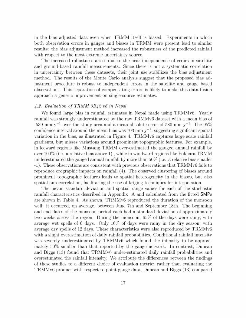
4.2. Evaluation of TRMM 3B42 v6 in Nepal
We found large bias in rainfall estimates in Nepal made using TRMMv6. Yearlyrainfall was strongly underestimated by the raw TRMMv6 dataset with a mean bias of-539 mm y−1 over the study area and a mean absolute error of 580 mm y−1. The 95%confidence interval around the mean bias was 703 mm y−1, suggesting significant spatialvariation in the bias, as illustrated in Figure 4. TRMMv6 captures large scale rainfallgradients, but misses variations around prominent topographic features. For example,in leeward regions like Mustang TRMM over-estimated the gauged annual rainfall byover 100% (i.e. a relative bias above 1) , while in windward regions like Pokhara TRMMunderestimated the gauged annual rainfall by more than 50% (i.e. a relative bias smaller-1). These observations are consistent with previous observations that TRMMv6 fails toreproduce orographic impacts on rainfall (4). The observed clustering of biases aroundprominent topographic features leads to spatial heterogeneity in the biases, but alsospatial autocorrelation, facilitating the use of kriging techniques for interpolation.
The mean, standard deviation and spatial range values for each of the stochasticrainfall characteristics described in Appendix A and calculated from the fitted SMPsare shown in Table 4. As shown, TRMMv6 reproduced the duration of the monsoonwell: it occurred, on average, between June 7th and September 18th. The beginningand end dates of the monsoon period each had a standard deviation of approximatelytwo weeks across the region. During the monsoon, 65% of the days were rainy, withaverage wet spells of 6 days. Only 16% of days were rainy in the dry season, withaverage dry spells of 12 days. These characteristics were also reproduced by TRMMv6with a slight overestimation of daily rainfall probabilities. Conditional rainfall intensitywas severely underestimated by TRMMv6 which found the intensity to be approxi-mately 50% smaller than that reported by the gauge network. In contrast, Duncanand Biggs (13) found that TRMMv6 under-estimated daily rainfall probabilities andoverestimated the rainfall intensity. We attribute the differences between the findingsof these studies to a different choice of evaluation metric: rather than evaluating theTRMMv6 product with respect to point gauge data, Duncan and Biggs (13) compared
17

TRMMv6 to interpolated daily precipitation measurements. As discussed in section4.4.2, errors associated with spatial interpolation of rainfall gauges exceed the errorsources in TRMMv6 in regions with low gauge densities. Because of such embedded in-terpolation errors, the evaluation of TRMMv6 against gridded precipitation stemmingfrom interpolated gauge data is problematic.
4.3. Stochastic modeling of Nepalese rainfall
Applying the stochastic model described in section 2.1 to rain gauge data in Nepallead to a mean absolute error in the annual rainfall of 7.8 mm y−1 compared to theobserved time series – 0.4% of the region’s average annual rainfall of 1754 mm y−1.Evaluating the stochastic model for each TRMM pixel as illustrated for one gauge inFigure 3 lead to a mean absolute error of the same order. These results suggest thatdespite the complexity of Himalayan precipitation processes the local daily rainfall waswell described by a simple seasonal parametric model.
4.4. Performance of the Bias Adjustment Method in Nepal
4.4.1. Performance at Gauged Pixels
Adjusting the SMPs at TRMMv6 pixels that contain gauges (Section 3.2.4) reducedthe mean error in annual rainfall to -9 mm y−1 (90% CI: 30 mm y−1), effectivelyeliminating it. The mean absolute error between gauges and corrected TRMMv6 pixelswas reduced by a factor of 45%, from 580 mm y−1 to 319 mm y−1. The fact that somuch error remains in the MAE indicates significant outlier compensation effects. Thatis, the biases are eliminated on average, but remain locally important.
4.4.2. Annual Rainfall at Ungauged Pixels
Figure 5 shows the results of the cross validation procedure described in section3.2.5, which illustrates the ability of the bias adjustment method to reproduce yearlyrainfall at ungauged locations. Comparing raw TRMMv6 and TRMMv7 to gaugesresults in MAEs of 580 mm y−1 and 404 mm y−1 respectively. These values compareto a MAE of 443 mm y−1 obtained when interpolating SMPs from all available gauges.Thus, interpolating the existing gauge network in Nepal outperforms TRMMv6 in theestimation of local annual rainfall, but is surpassed by TRMMv7. The MAE relatedto gauge interpolation increases steadily with decreasing gauge network density, andexceeds that of the unadjusted TRMMv6 for densities below 2 gauges per 10,000 km2;that is, an average distance between gauges of about 70km. Using all the gauges in thetraining set (i.e. 80% of the total number of gauges) to adjust the bias on TRMMv6reduced the mean absolute error in annual rainfall to 391 mm y−1. This represents22% of the region’s average gauged rainfall of 1753 mm y−1 estimated through Thiessenpolygons (section 3.2.1). When considering the perhaps more accurate measure ofaverage rainfall of 1233 mm y−1 obtained by adjusting TRMMv6 over the whole studyarea, the relative error increases to 31%. This includes the effect of errors related toaggregation and spatial interpolation to ungauged TRMMv6 pixels.
18

4.4.3. Decreasing Returns to Network Density
The error curve for the bias adjustment on annual rainfall is shown in Figure 5 (a).This curve flattens and asymptotes to the error curve for the TRMMv7 data when allavailable gauges are used to correct TRMMv6. This is consistent with the large num-ber of gauges used by TRMMv7 to adjust the remote sensing rainfall estimates. Theflattening of the error curve leads to two noteworthy implications. (i) The incrementalbenefit of adding gauges to the network to adjust TRMMv6 decreases with increas-ing network density. The curvature appears to be highest at a density of about 2.5gauges per 10,000 km2, where the error is decreased to 458 mm y−1, that is 36% ofthe TRMM-adjusted average rainfall using only 25% of the available gauges. Thus, arelatively sparse network of gauges, integrated in a bias adjustment procedure based on10 parameters, efficiently corrects TRMMv6 and generates performance levels compa-rable to TRMMv7. (ii) The hypothetical availability of a dense gauge network – e.g.observed data for every TRMM pixel – to adjust TRMMv6 would result in a non-zeroasymptotic error. Indeed, TRMMv7, which is calibrated on 280 gauges, does not out-perform a bias adjusted TRMMv6 that uses only 91 gauges. The asymptotic error of319 mm y−1 was estimated using the complete set of available gauges as training andvalidation sets simultaneously, overriding the aggregation and interpolation steps of theprocedure. This residual error is related to omission of local rainfall variations by thecoarse resolution of the TRMM satellite and spacing of the Nepalese gauges.
4.4.4. Rainfall Variance and Occurrence Probability
Figure 5 (b) and 5 (c) show the method’s performance at predicting rainfall vari-ance and occurrence using the same cross validation approach as Section 4.4.2. Forthe variance of daily rainfall, the performance of TRMMv7 was reached by correctingTRMMv6 using a small subset of the gauge network. Increasing the density of gaugesonly slightly improved the performance of gauge-based techniques.
When considering rainfall occurrence, gauge interpolation outperformed both TR-MMv6 and TRMMv7 by nearly 30%, with an average error of 21 rainy days per yearwhen all gauges were used. This is consistent with the fact that the TRMM algorithmcalibrates remote sensing data using observed monthly mean precipitations, which cor-rects for average rainfall intensity but fails to adjust biases on rainfall occurrence. Theerror curve corresponding to the bias adjustment procedure follows the curve relatedto gauge interpolation, showing that the proposed bias adjustment method successfullycorrects rainfall occurrence. Similar to yearly rainfall, the error curve on rainfall oc-currence flattens, again suggesting that the incremental benefit of adding gauges to thenetwork to adjust TRMMv6 decreases with increasing network density.
4.4.5. TRMMv7 vs. Bias-Adjusted TRMMv6
Despite the availability in Nepal of high quality TRMMv7 data that successfully rep-resents annual rainfall, the proposed approach to correct TRMMv6 finds its usefulness
19
in its parsimony and its ability to correct hydrologically relevant rainfall statistics usinga much sparser gauge network. Our approach reached the performance of TRMMv7in the prediction of annual rainfall using a small subset (90 gauges) of the 280 gaugesused in the GPCC dataset to calibrate TRMMv7. Including a stochastic model in theapproach allows the daily rainfall to be corrected by adjusting 10 stationary parame-ters, instead of the 144 monthly means calibrated by the TRMM algorithm for eachpixel over a period of 12 years. The proposed method reaches the prediction of rainfallvariance and significantly improves that of rainfall occurrence in ungauged locations rel-ative to TRMM v7, using only a subset of the gauges. Finally, we have shown that ourmethod enables even a sparse ground gauge network to correct satellite observations tothe same level of accuracy as achieved by monthly-interpolation from a dense network,suggesting that our approach will have applicability in sparsely monitored locations.
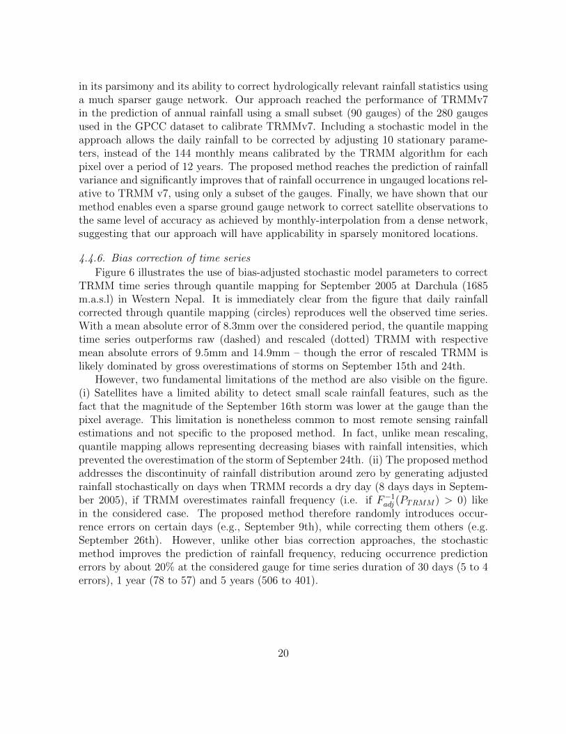
4.4.6. Bias correction of time series
Figure 6 illustrates the use of bias-adjusted stochastic model parameters to correctTRMM time series through quantile mapping for September 2005 at Darchula (1685m.a.s.l) in Western Nepal. It is immediately clear from the figure that daily rainfallcorrected through quantile mapping (circles) reproduces well the observed time series.With a mean absolute error of 8.3mm over the considered period, the quantile mappingtime series outperforms raw (dashed) and rescaled (dotted) TRMM with respectivemean absolute errors of 9.5mm and 14.9mm – though the error of rescaled TRMM islikely dominated by gross overestimations of storms on September 15th and 24th.
However, two fundamental limitations of the method are also visible on the figure.(i) Satellites have a limited ability to detect small scale rainfall features, such as thefact that the magnitude of the September 16th storm was lower at the gauge than thepixel average. This limitation is nonetheless common to most remote sensing rainfallestimations and not specific to the proposed method. In fact, unlike mean rescaling,quantile mapping allows representing decreasing biases with rainfall intensities, whichprevented the overestimation of the storm of September 24th. (ii) The proposed methodaddresses the discontinuity of rainfall distribution around zero by generating adjustedrainfall stochastically on days when TRMM records a dry day (8 days days in Septem-ber 2005), if TRMM overestimates rainfall frequency (i.e. if F−1adj (PTRMM) > 0) likein the considered case. The proposed method therefore randomly introduces occur-rence errors on certain days (e.g., September 9th), while correcting them others (e.g.September 26th). However, unlike other bias correction approaches, the stochasticmethod improves the prediction of rainfall frequency, reducing occurrence predictionerrors by about 20% at the considered gauge for time series duration of 30 days (5 to 4errors), 1 year (78 to 57) and 5 years (506 to 401).
20
5. Conclusion
This study explored the potential for bias correction techniques based on stochas-tic rainfall representations to provide spatially aggregated rainfall data with value fordriving hydrological simulations. We have demonstrated that such methods are robustto multiple sources of error and bias in both satellite and ground-based observationsof rainfall, and provide robust results for gauge densities as low as 2.5 per 10,000 km2.We have illustrated that by separating out sources of rainfall observation bias whichhave different directionalities in different spatial locations, this methodology not onlyprovides a reproduction of rainfall totals which compares to alternative bias correctionapproaches, such as that applied by NASA for the TRMMv7 dataset; but actually repro-duces important statistical features of the rainfall time series, notably the local rainfallvariance and rainfall occurrence probabilities, with greater fidelity than obtained fromconventional time series bias adjustments.
While a fundamental limitation lies in the inability of satellites to observe small scalerainfall features (a limitation common to other bias adjustment approaches, as shown bythe convergence of error estimates between the stochastic approach and the TRMMv7observations), the proposed method successfully generates parametric distributions ofbias-corrected rainfall using a finite number of gauges. Useful application of these resultsinclude their use as inputs to frequency domain hydrological models, the stochasticgeneration of synthetic rainfall or the correction of remotely sensed time series throughquantile mapping.
Thus, the stochastic procedure effectively combines satellite data with sparse raingauges, providing a robust technique for estimating rainfall properties in minimally-gauged regions, and offering insight into the minimal rainfall gauge network that couldbe reliably used to understand the spatio-temporal variations in precipitation in moun-tainous regions.
6. Acknowledgement
The authors would like to thank Michele Muller for her invaluable assistance indata analysis and coding, as well as Slav Hermanowicz and anonymous reviewers fortheir helpful review and comments. Data have been graciously provided by the NASATropical Rainfall Measurement Mission, the Department of Hydrology and Meteorol-ogy of Nepal and the HKH-FRIEND project. The Fulbright Science and TechnologyFellowship and the National Science Foundation NSF EAR-1013339 are gratefully ac-knowledged for funding.
21

References
[1] Soni Yatheendradas, Thorsten Wagener, Hoshin Gupta, Carl Unkrich, David Goodrich,Mike Schaffner, and Anne Stewart. Understanding uncertainty in distributed flashflood forecasting for semiarid regions. Water Resources Research, 44(5), 2008.doi:10.1029/2007WR005940.
[2] S.R. Kansakar, D.M. Hannah, J. Gerrard, and G. Rees. Spatial pattern in the precip-itation regime of Nepal. International Journal of Climatology, 24(13):1645–1659, 2004.doi:10.1002/joc.1098.
[3] G.J. Huffman, D.T. Bolvin, E.J. Nelkin, D.B. Wolff, R.F. Adler, G. Gu, Y. Hong, K.P.Bowman, and E.F. Stocker. The TRMM multisatellite precipitation analysis (TMPA):Quasi-global, multiyear, combined-sensor precipitation estimates at fine scales. Journalof Hydrometeorology, 8(1):38–55, 2007. doi:10.1175/JHM560.1.
[4] Y Chen, E.E. Ebert, K.J.E. Walsh, and N.E. Davidson. Evaluation of TRMM 3b42precipitation estimates of tropical cyclone rainfall using PACRAIN data. Journal ofGeophysical Research: Atmospheres, 2013. doi:10.1002/jgrd.50250.
[5] C. Andermann, S. Bonnet, and R. Gloaguen. Evaluation of precipitation data setsalong the Himalayan front. Geochemistry Geophysics Geosystems, 12(7):Q07023, 2011.doi:10.1029/2011GC003513.
[6] B. Bookhagen and D.W. Burbank. Topography, relief, and TRMM-derived rainfallvariations along the Himalayas. Geophysical Research Letters, 33(8):L08405, 2006.doi:10.1029/2006GL026037.
[7] M.S. Shrestha. Bias-Adjustment of Satellite-Based Rainfall Estimates over the CentralHimalayas of Nepal for Flood Prediction. PhD thesis, Kyoto University, 2011.
[8] E. Ward, W. Buytaert, L. Peaver, and H. Wheater. Evaluation of precipitation productsover complex mountainous terrain: A water resources perspective. Advances in WaterResources, 34(10):1222–1231, 2011. doi:10.1016/j.advwatres.2011.05.007.
[9] M.N. Islam, S. Das, and H. Uyeda. Calibration of TRMM derived rainfall overNepal during 1998–2007. The Open Atmospheric Science Journal, 4:12–23, 2010.doi:10.2174/1874282301004010012.
[10] Z.Y. Yin, X. Zhang, X. Liu, M. Colella, and X. Chen. An assessment of the bi-ases of satellite rainfall estimates over the Tibetan Plateau and correction meth-ods based on topographic analysis. Journal of Hydrometeorology, 9(3):301–326, 2008.doi:10.1175/2007JHM903.1.
[11] M.J.M. Cheema and W.G.M. Bastiaanssen. Local calibration of remotely sensedrainfall from the TRMM satellite for different periods and spatial scales in theIndus Basin. International Journal of Remote Sensing, 33(8):2603–2627, 2012.doi:10.1080/01431161.2011.617397.
22

[12] L. Gudmundsson, J.B. Bremnes, J.E. Haugen, and T. Engen Skaugen. Technical note:Downscaling RCM precipitation to the station scale using quantile mapping – a compar-ison of methods. Hydrol. Earth Syst. Discuss., 9:6185–6201, 2012. doi:10.5194/hessd-9-6185-2012.
[13] J. Duncan and E.M. Biggs. Assessing the accuracy and applied use of satellite-derived precipitation estimates over Nepal. Applied Geography, 34:626–638, 2012.doi:10.1016/j.apgeog.2012.04.001.
[14] F Laio, A Porporato, L Ridolfi, and Ignacio Rodriguez-Iturbe. Plants in water-controlledecosystems: Active role in hydrologic processes and response to water stress: Ii. proba-bilistic soil moisture dynamics. Advances in Water Resources, 24(7):707–723, 2001.
[15] G. Botter, A. Porporato, I. Rodriguez-Iturbe, and A. Rinaldo. Basin-scale soil mois-ture dynamics and the probabilistic characterization of carrier hydrologic flows: Slow,leaching-prone components of the hydrologic response. Water Resources Research, 43(2):2417, 2007. doi:10.1029/2006WR005043.
[16] R. Srikanthan and T.A. McMahon. Stochastic generation of annual, monthly and dailyclimate data: A review. Hydrology and Earth System Sciences, 5(4):653–670, 2001.doi:10.5194/hess-5-653-2001.
[17] C.W. Richardson. Stochastic simulation of daily precipitation, temperature, and solar ra-diation. Water Resources Research, 17(1):182–190, 1981. doi:10.1029/WR017i001p00182.
[18] O.D. Jimoh and P. Webster. The optimum order of a Markov chain model for dailyrainfall in Nigeria. Journal of Hydrology, 185(1):45–69, 1996. doi:10.1007/s00704-008-0051-3.
[19] D.S. Wilks. Multisite generalization of a daily stochastic precipitation generation model.Journal of Hydrology, 210(1):178–191, 1998. doi:10.1016/S0022-1694(98)00186-3.
[20] F.P. Brissette, M. Khalili, and R. Leconte. Efficient stochastic generation ofmulti-site synthetic precipitation data. Journal of Hydrology, 345(3):121–133, 2007.doi:10.1016/j.jhydrol.2007.06.035.
[21] G.J. Huffman and D.T. Bolvin. Trmm and other data precipitation data set documen-tation. Technical report, Mesoscale Atmospheric Processes Laboratory, NASA GoddardSpace Flight Center, 2013.
[22] Ignacio Rodriguez-Iturbe and Jose M Mejıa. On the transformation of pointrainfall to areal rainfall. Water Resources Research, 10(4):729–735, 1974.doi:10.1029/WR010i004p00729.
[23] Edzer J. Pebesma. Multivariable geostatistics in S: the gstat package. Computers andGeosciences, 30:683–691, 2004. doi:10.1016/j.cageo.2004.03.012.
23
[24] P.J Ribeiro and P.J Diggle. geoR: a package for geostatistical analysis. R-NEWS, 1(2):14–18, June 2001. URL http://CRAN.R-project.org/doc/Rnews/. ISSN 1609-3631.
[25] J. Shao and D. Tu. The Jackknife and Bootstrap. Springer-Verlag, New York, 1995.
[26] R. Ihaka and R. Gentleman. R: A language for data analysis and graph-ics. Journal of Computational and Graphical Statistics, 5(3):299–314, 1996.doi:10.1080/10618600.1996.10474713.
[27] NASA and JAXA. http://asterweb.jpl.nasa.gov/gdem.asp, January 2013.
[28] W.W. Immerzeel, L.P.H. van Beek, and M.F.P. Bierkens. Climate change will affect theAsian water towers. Science, 328(5984):1382–1385, 2010. doi:10.1126/science.1183188.
[29] B.C. Bhatt and K. Nakamura. Characteristics of monsoon rainfall around the Himalayasrevealed by TRMM precipitation radar. Monthly Weather Review, 133(1):149–165, 2005.doi:10.1175/MWR-2846.1.
[30] A.M. Anders, G.H. Roe, B. Hallet, D.R. Montgomery, N.J. Finnegan, and J. Putkonen.Spatial patterns of precipitation and topography in the Himalaya. Special Papers -Geological Society of America, 398:39, 2006. doi:10.1130/2006.2398(03).
[31] A.P. Barros, M. Joshi, J. Putkonen, and D.W. Burbank. A study of the 1999monsoon rainfall in a mountainous region in central Nepal using TRMM productsand rain gauge observations. Geophysical Research Letters, 27(22):3683–3686, 2000.doi:10.1029/2000GL011827.
[32] M.K. Yamamoto, K. Ueno, and K. Nakamura. Comparison of satellite precipitationproducts with rain gauge data for the Khumb region, Nepal Himalayas. Journal of theMeteorological Society of Japan, 89(6):597–610, 2011. doi:10.2151/jmsj.2011-601.
[33] Satya Prakash, C Mahesh, and RM Gairola. Comparison of TRMM Multi-satellite Precipitation Analysis (TMPA)-3B43 version 6 and 7 products with raingauge data from ocean buoys. Remote Sensing Letters, 4(7):677–685, 2013.doi:10.1080/2150704X.2013.783248.
[34] HKH-FRIEND. http://www.hkh-friend.net.np/rhdc.html, August 2011.
[35] Department of Hydrology and Meteorology. Kathmandu, September 2011.
[36] NASA. http://mirador.gsfc.nasa.gov, November 2012.
[37] W.N. Venables and B.D. Ripley. Modern applied statistics with S. Springer-Verlag, NewYork, 2002.
24

7. Tables
SMP Stochastic Model ParameterMAE Mean Absolute ErrorX Daily PrecipitationP Probability of daily precipitation occurrenceNp Number of gauges in the considered pixelNg Number of gauges to interpolate fromNMC Number of Monte Carlo roundsNCV Number of Cross Validation roundsai Fraction of pixel occupied by the Thiessen polygon of gauge i
v(param)i Interpolation weight associated to gauge i and parameter paramC(d) Correction factor on variance for areal rainfall on in a pixel of diagonal d
i Subscript for gauges (point rainfall)
pt Subscript for pixels aggregated from gauges (point rainfall)
pix Subscript for pixels aggregated from gauges (areal rainfall)
TRMM Subscript for TRMM pixelswet Subscript for rainy days
j Subscript for Monte Carlo or Cross Validation rounds
Table 1: Acronyms, variables and subscripts
P(w)01 Probability of a dry day being followed by a wet day in the wet season
P(d)01 Probability of a dry day being followed by wet day in the dry season
P(w)11 Probability of a wet day being followed by wet day in the wet season
P(d)11 Probability of a dry day being followed by wet day in the wet season
GS(w) Gamma shape parameter for daily rainfall depth in the wet season
GS(d) Gamma shape parameter for daily rainfall depth in the dry season
GR(w) Gamma rate parameter for daily rainfall depth in the wet season
GR(d) Gamma rate parameter for daily rainfall depth in the dry seasonRnStr Average calendar day when Monsoon startsRnStp Average calendar day when Monsoon ends
Table 2: Stochastic Model Parameters (SMP).
25
Variable Default Value Experimental Range
fAWNlocal 0 0 - 0.2N 50 10 - 1000
zmax 8848 1000 - 8848fAWNobs 0 0 - 0.3
fBIASmean 1 0.5 - 5fBIASrange 1 0.01 - 2
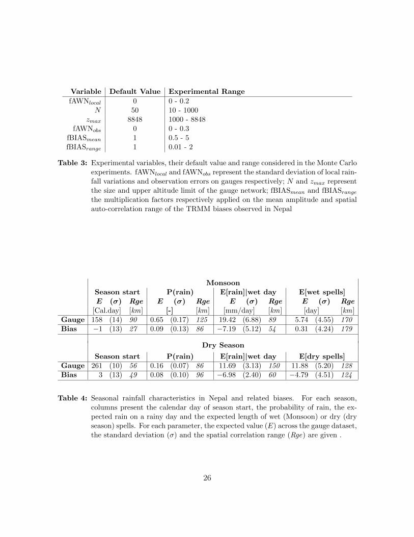
Table 3: Experimental variables, their default value and range considered in the Monte Carloexperiments. fAWNlocal and fAWNobs represent the standard deviation of local rain-fall variations and observation errors on gauges respectively; N and zmax representthe size and upper altitude limit of the gauge network; fBIASmean and fBIASrange
the multiplication factors respectively applied on the mean amplitude and spatialauto-correlation range of the TRMM biases observed in Nepal
MonsoonSeason start P(rain) E[rain]|wet day E[wet spells]E (σ) Rge E (σ) Rge E (σ) Rge E (σ) Rge
[Cal.day] [km] [-] [km] [mm/day] [km] [day] [km]Gauge 158 (14) 90 0.65 (0.17) 125 19.42 (6.88) 89 5.74 (4.55) 170Bias −1 (13) 27 0.09 (0.13) 86 −7.19 (5.12) 54 0.31 (4.24) 179
Dry Season
Season start P(rain) E[rain]|wet day E[dry spells]Gauge 261 (10) 56 0.16 (0.07) 86 11.69 (3.13) 150 11.88 (5.20) 128Bias 3 (13) 49 0.08 (0.10) 96 −6.98 (2.40) 60 −4.79 (4.51) 124
Table 4: Seasonal rainfall characteristics in Nepal and related biases. For each season,columns present the calendar day of season start, the probability of rain, the ex-pected rain on a rainy day and the expected length of wet (Monsoon) or dry (dryseason) spells. For each parameter, the expected value (E) across the gauge dataset,the standard deviation (σ) and the spatial correlation range (Rge) are given .
26

8. Figures
27

7. Figures
(a)
(b)
0e+00
1e 04
2e 04
3e 04
4e 04
0 2000 4000 6000Altitude (m.a.s.l)
Den
sity
Rain GaugesTerrain
(c)
Figure 1: Study region and available data. (a) Location of the available gauges and meanannual rainfall. The figure shows vast zones in the North that are not coveredby the gauge network. The di !erence in annual rainfall between Pokhara (P)and Mustang (M), two proximate regions separated by the Annapurna range,illustrates the importance of rain shadow e !ects. (b) TRMMv6 measured yearlyrainfall in 2010, showing decreasing trends towards the east and north. (c) Kerneldensity estimates of the altitude distributions of the area and of the rain gauges.The figure shows that the altitude distribution of the area is bimodal with modesat 1000 masl and 5000 masl. This distribution is not matched by the gauges,which are preferentially located below 3000 masl.
21
D
Figure 1: Study region and available data. (a) Location of the available gauges and mean an-nual rainfall. The figure shows vast zones in the North that are not covered by thegauge network. The difference in annual rainfall between Pokhara (P) and Mus-tang (M), two proximate regions separated by the Annapurna range, illustrates theimportance of rain shadow effects. The example of time series correction describedin Section 3.2.6 focuses on the rainfall gauge at Darchula (D) in western Nepal.(b) Yearly rainfall in 2010 measured by TRMM 3B43 v6 (monthly precipitation)and aggregated annually, showing decreasing trends towards the east and north.(c) Kernel density estimates of the altitude distributions of the area and of therain gauges. The figure shows that the altitude distribution of the area is bimodalwith modes at 1000 masl and 5000 masl. This distribution is not matched by thegauges, which are preferentially located below 3000 masl.
28

25%50%75%
100%
0.0
0.5
1.0
1.5
2.0
0 2000 4000 6000 8000Maximum Gauge Altitude (m.a.s.l)
MAE
/ M
AE(8
848)
(a)
02468
10
0.0 0.1 0.2 0.3Noise factor on gauges
MAE
/ M
AE(0
)
(b)
02468
1012
0 1 2 3 4 5Multiplic. factor on mean TRMM bias
MAE
/ M
AE(0
)
(c)
02468
10
0.00 0.05 0.10 0.15 0.20Noise factor on local rainfall
MAE
/ M
AE(0
)
(d)
Figure 2: Monte-Carlo simulation of the e↵ects of uncertainty sources on the estimatedannual rainfall for the bias adjustment method (squares) and the two controlmethods: unadjusted TRMM (triangles) and interpolation from gauges (circles).The vertical axis represents the mean absolute error on annual rainfall, normalizedby its value at the default state described in Table 3. (a) E↵ect of the systematicselection of low altitude gauges: the x axis represents the lower altitude limit set forthe randomly selected gauge locations; the graph line without point markers andsecondary y axis represent the cumulative altitude distribution of the study area.(b) E↵ect of the variance of the random observation errors on SMPs observedat synthetic gauges. (c) E↵ect of the mean amplitude of the TRMM bias. (d)E↵ect of the variance of local random rainfall variations occurring at a spatialscale smaller than that being captured by the gauge network.
22
0
2
4
6
8
10
0.00.10.20.3Noise factor on gauges
MAE
/ M
AE(0
)
Data SourceBias Corrected TRMMGauge interpolationRaw TRMM
Bias Corrected TRMM
0
2
4
6
8
10
0.00.10.20.3Noise factor on gauges
MAE
/ M
AE(0
)
Data SourceBias Corrected TRMMGauge interpolationRaw TRMMGauge Interpolation
0
2
4
6
8
10
0.00.10.20.3Noise factor on gauges
MAE
/ M
AE(0
)
Data SourceBias Corrected TRMMGauge interpolationRaw TRMMRaw TRMM
Figure 2: Monte-Carlo simulation of the effects of uncertainty sources on the estimatedannual rainfall for the bias adjustment method (squares) and the two controlmethods: unadjusted TRMM (triangles) and interpolation from gauges (circles).The vertical axis represents the mean absolute error on annual rainfall, normalizedby its value at the default state described in Table 3. (a) Effect of the systematicselection of low altitude gauges: the x axis represents the lower altitude limit set forthe randomly selected gauge locations; the graph line without point markers andsecondary y axis represent the cumulative altitude distribution of the study area.(b) Effect of the variance of the random observation errors on SMPs observedat synthetic gauges. (c) Effect of the mean amplitude of the TRMM bias. (d)Effect of the variance of local random rainfall variations occurring at a spatialscale smaller than that being captured by the gauge network.
29

0 100 300
050
150
Calendar Day
Prec
ipita
tion
(mm
)
(a)
Rainfall (mm/d)
Den
sity
0 50 1000.00
0.04
0.08
(b)
0 4 8 12
020
4060
Dry spell length (days)
Spel
l cou
nt
(c)
0 5 15
020
40
Wet spell length (days)
Spel
l cou
nt
(d)
Figure 3: Stochastic rainfall parametrization at a gauge in Western Nepal (Lat:29�28’,Long:80�32’, z=1266m). (a) A step function is fitted to the time series of dailyrainfall to determine seasonality. Monsoon starts and ends at calendar days, whenthe step function is vertical. (b) A two-parameter gamma distribution is fittedon daily rainfall intensity for each season. The fit on Monsoon rainfall is rep-resented in the figure. (c) The distribution of dry spells (here during the dry
season) matches a geometric distribution with probability P(d)01 . (d) The distri-
bution of wet spells (here during the Monsoon) matches a geometric distribution
with probability P(w)11 .
Figure 4: Spatial repartition of the TRMM bias on yearly rainfall. The relative bias iscalculated by normalizing the observed bias by the yearly rainfall measured at thegauge. A relative bias of -1 means that the average yearly rainfall observed at thegauge is double the value given by the covering TRMM pixel. The large variationand di↵erent signs between Pokhara (P) and Mustang (M), two proximate regionsseparated by the Anapurna Range illustrates the e↵ect of rain shadows on thebias.
23
Figure 3: Stochastic rainfall parametrization at a gauge in Western Nepal (Lat:29◦28’,Long:80◦32’, z=1266m). (a) A step function is fitted to the time series of dailyrainfall to determine seasonality. Monsoon starts and ends at calendar days, whenthe step function is vertical. (b) A two-parameter gamma distribution is fittedon daily rainfall intensity for each season. The fit on Monsoon rainfall is rep-resented in the figure. (c) The distribution of dry spells (here during the dry
season) matches a geometric distribution with probability P(d)01 . (d) The distri-
bution of wet spells (here during the Monsoon) matches a geometric distribution
with probability P(w)11 .
Figure 4: Spatial repartition of the TRMM bias on yearly rainfall. The relative bias iscalculated by normalizing the observed bias by the yearly rainfall measured at thegauge. A relative bias of -1 means that the average yearly rainfall observed at thegauge is double the value given by the covering TRMM pixel. The large variationand different signs between Pokhara (P) and Mustang (M), two proximate regionsseparated by the Anapurna Range illustrates the effect of rain shadows on thebias.
30

0
200
400
600
0.0 2.5 5.0 7.5 10.0 12.5Gauge Density (10,000km−2)
MAE
(mm
/yr)
Gauge Interpolation
Bias Corrected TRMMv6
Raw TRMMv6
Raw TRMMv7
(a) Annual Rainfall
0
50
100
0.0 2.5 5.0 7.5 10.0 12.5Gauge Density (10,000km−2)
MA
E (m
md)
2
(b) Rainfall Variance
0
10
20
30
40
0.0 2.5 5.0 7.5 10.0 12.5Gauge Density (10,000km−2)
MA
E (d
yr)
(c) Rainfall Occurence
Figure 5: Cross validation performances of TRMMv6 (white circles), TRMMv7 (black cir-cles), gauge interpolation (crosses) and bias adjusted TRMMv6 (crossed circles).(a) Mean absolute error on yearly rainfall prediction at ungauged location: bias ad-justed TRMMv6 outperforms raw TRMMv6 and gauge interpolation and reachesthe performance of TRMMv7 at gauge densities of 6 gauges per 10,000 km2. (b)Mean absolute error on the variance of daily rainfall: Correcting TRMMv6 leads toequivalent performances than TRMMv7 and both datasets outperform TRMMv6.(c) Mean absolute error on the prediction of the average number of rainy days peryear: Gauges outperform both TRMM dataset and improve the performance ofbias adjusted TRMMv6.
31

Sep 04 Sep 09 Sep 14 Sep 19 Sep 24 Sep 29
020
4060
80
2005
Rai
nfal
l (m
m/d
)
GaugeTRMM: Quantile MappingTRMM: RawTRMM: Scaled Mean
Figure 6: Application of the bias-adjusted stochastic model parameters in a quantile map-ping procedure to correct daily rainfall time series at Darchula (1683 m.a.s.l) inWestern Nepal. The ability of the TRMMv6 time series adjusted with the proposedmethod (solid) to reproduce gauged values (shaded) exceeded the performance ofraw TRMMv6 (dashed) and that of rescaled TRMMv6 (dotted) – i.e. adjustedwithout stochastic model parameters .
32

Appendix A. From stochastic model parameters to evaluation metrics
The output of our stochastic model are the 10 parameters described in Table 2.Combining these parameters, one can obtain seasonal metrics such as the unconditionalexpectation and variance of daily rainfall (E
[X(i)
], Var
(X(i)
)) the expected length of
wet and dry spells (L(i)w , L
(i)d ) and the probability of rainfall occurring on any given day
(P (i)). These relationships are listed in equations A.1-A.5:
L(i)w =
1
1− P (i)11
(A.1)
L(i)d =
1
P(i)01
(A.2)
P (i) =P i01
1 + P(i)01 − P
(i)11
(A.3)
E[X(i)
]= P (i)GS
GR(A.4)
Var(X(i)
)= P (i) GS
GR2 + P (i)(1− P (i))GS
GR(A.5)
where the subscript i indicates either the wet (w) or dry (d) season. By weighingseasonal metrics by the duration of the corresponding season we get the annual metrics(Lw, P , E [X] and Var (X)):
P = LRnP(w) + (1− LRn)P
(d) (A.6)
Lw =
(1− LRnP
(w)P(w)11 + (1− LRn)P
(d)P(d)11
P
)−1(A.7)
E [X] = LRnP(w)GS
(w)
GR(w)+ (1− LRn)P
(d)GS(d)
GR(d)(A.8)
Var (X) = LRn
(GS(w)
GR(w)
)2
+ (1− LRn)
(GS(d)
GR(d)
)2
−
(LRn
GS(w)
GR(w)+ (1− LRn)
GS(d)
GR(d)
)2
+ LRnGS(w)
GR2(w)
+ (1− LRn)GS(d)
GR2(d)
(A.9)
(A.10)
with LRn = (RnStp−RnStr)/365, the fraction of the year occupied by the rainy season.Finally, yearly rainfall and the average number of rainy days per year can easily be
33
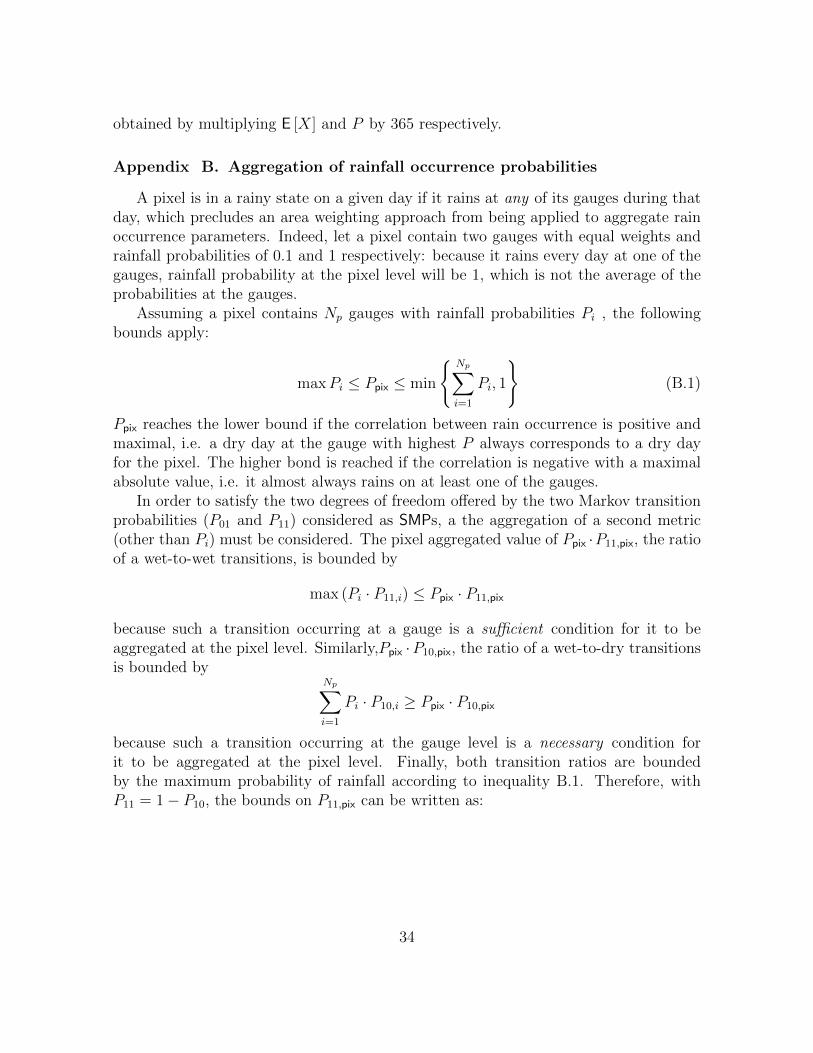
obtained by multiplying E [X] and P by 365 respectively.
Appendix B. Aggregation of rainfall occurrence probabilities
A pixel is in a rainy state on a given day if it rains at any of its gauges during thatday, which precludes an area weighting approach from being applied to aggregate rainoccurrence parameters. Indeed, let a pixel contain two gauges with equal weights andrainfall probabilities of 0.1 and 1 respectively: because it rains every day at one of thegauges, rainfall probability at the pixel level will be 1, which is not the average of theprobabilities at the gauges.
Assuming a pixel contains Np gauges with rainfall probabilities Pi , the followingbounds apply:
maxPi ≤ Ppix ≤ min
{Np∑i=1
Pi, 1
}(B.1)
Ppix reaches the lower bound if the correlation between rain occurrence is positive andmaximal, i.e. a dry day at the gauge with highest P always corresponds to a dry dayfor the pixel. The higher bond is reached if the correlation is negative with a maximalabsolute value, i.e. it almost always rains on at least one of the gauges.
In order to satisfy the two degrees of freedom offered by the two Markov transitionprobabilities (P01 and P11) considered as SMPs, a the aggregation of a second metric(other than Pi) must be considered. The pixel aggregated value of Ppix ·P11,pix, the ratioof a wet-to-wet transitions, is bounded by
max (Pi · P11,i) ≤ Ppix · P11,pix
because such a transition occurring at a gauge is a sufficient condition for it to beaggregated at the pixel level. Similarly,Ppix ·P10,pix, the ratio of a wet-to-dry transitionsis bounded by
Np∑i=1
Pi · P10,i ≥ Ppix · P10,pix
because such a transition occurring at the gauge level is a necessary condition forit to be aggregated at the pixel level. Finally, both transition ratios are boundedby the maximum probability of rainfall according to inequality B.1. Therefore, withP11 = 1− P10, the bounds on P11,pix can be written as:
34
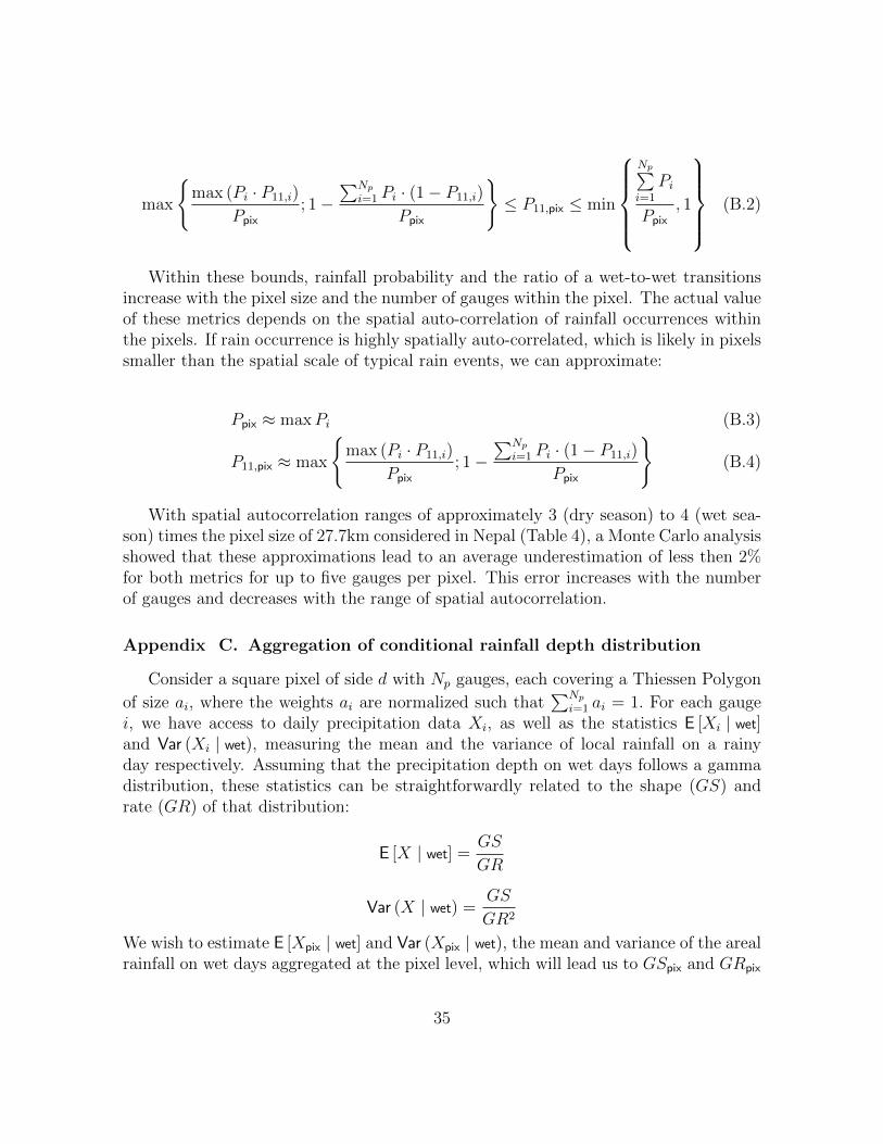
max
{max (Pi · P11,i)
Ppix; 1−
∑Np
i=1 Pi · (1− P11,i)
Ppix
}≤ P11,pix ≤ min
Np∑i=1
Pi
Ppix, 1
(B.2)
Within these bounds, rainfall probability and the ratio of a wet-to-wet transitionsincrease with the pixel size and the number of gauges within the pixel. The actual valueof these metrics depends on the spatial auto-correlation of rainfall occurrences withinthe pixels. If rain occurrence is highly spatially auto-correlated, which is likely in pixelssmaller than the spatial scale of typical rain events, we can approximate:
Ppix ≈ maxPi (B.3)
P11,pix ≈ max
{max (Pi · P11,i)
Ppix; 1−
∑Np
i=1 Pi · (1− P11,i)
Ppix
}(B.4)
With spatial autocorrelation ranges of approximately 3 (dry season) to 4 (wet sea-son) times the pixel size of 27.7km considered in Nepal (Table 4), a Monte Carlo analysisshowed that these approximations lead to an average underestimation of less then 2%for both metrics for up to five gauges per pixel. This error increases with the numberof gauges and decreases with the range of spatial autocorrelation.
Appendix C. Aggregation of conditional rainfall depth distribution
Consider a square pixel of side d with Np gauges, each covering a Thiessen Polygon
of size ai, where the weights ai are normalized such that∑Np
i=1 ai = 1. For each gaugei, we have access to daily precipitation data Xi, as well as the statistics E [Xi | wet]and Var (Xi | wet), measuring the mean and the variance of local rainfall on a rainyday respectively. Assuming that the precipitation depth on wet days follows a gammadistribution, these statistics can be straightforwardly related to the shape (GS) andrate (GR) of that distribution:
E [X | wet] =GS
GR
Var (X | wet) =GS
GR2
We wish to estimate E [Xpix | wet] and Var (Xpix | wet), the mean and variance of the arealrainfall on wet days aggregated at the pixel level, which will lead us to GSpix and GRpix
35

the aggregated parameters of our stochastic model.As a first step, we determine the local rainfall at a random point of the pixel Xpt
according a two-step data generating process as follows:(i) At the outset, before any measurements are made, a point of the pixel is chosen
uniformly at random. As a result, the area weights ai measure the probabilitythat this point is located in Thiessen Polygon i.
(ii) Subsequently, we assume that local rainfall across the entire Thiessen Polygon isconstant and measured by gauge i.
As a result, we can determine the expected unconditional rainfall at a random point ofthe pixel using the law of iterated expectation,
E [Xpt] = E [E [Xpt | i]] =
Np∑i=1
aiE [Xi] .
Here, E [Xpt | i] denotes the expected rainfall conditional on the random point being inPolygon i, in which case Xpt is equal to Xi by assumption. Knowing that the meanvalue over the pixel area of all possible realizations of the point process Xpt results inan areal rainfall process with an identical expectation (22) (i.e. E [Xpix] = E [Xpt]), wecan calculate the mean areal rainfall on a rainy day by applying the law of iteratedexpectations both at the pixel level and for each individual gauge,
E [Xpix | wet] =1
Ppix·
Np∑i=1
aiPiE [Xi | wet] . (C.1)
with Pi and Ppix the probability or rainfall at the gauge i and at the pixel level re-spectively and represent the expectations of the binomial stochastic processes definingrainfall occurrence at these points.
For the local variance, the same data generating process implies, by the law of totalvariance,
Var (Xpt) = E [Var (Xpt | i)] + Var (E [Xpt | i])= E [Var (Xi)] + E
[E [Xi]
2]− E [E [Xi]]2
=
Np∑i=1
aiVar (Xi) +
Np∑i=1
aiE [Xi]2 −
(Np∑i=1
aiE [Xi]
)2
Again, we condition on the polygon i and assume that precipitation is homogenous
36

within each Thiessen polygon (i.e. Xpt = Xi ). From equation C.1, we get:
Var (Xpt) =
Np∑i=1
aiVar (Xi) +
Np∑i=1
aiE [Xi]2 − P 2
pixE [Xpix | wet]2 (C.2)
In the next step, we condition on rainfall probability, applying the law of totalvariance and taking rainfall occurrence as a binomial random variable:
Var (Xi) = Var (E [Xi | wet]) + E [Var (Xi | wet)]= Pi(1− Pi)E [Xi | wet] + PiVar (Xi | wet) (C.3)
Substituting equation C.3 in equation C.2 we have:
(1− Ppix)PpixE [Xpix | wet] + PpixVar (Xpt | wet) =
= Pi(1− Pi)E [Xi | wet] + PiVar (Xi | wet) +
Np∑i=1
aiE [Xi]2 − P 2
pixE [Xpix | wet]2
Using equation C.1 to express PpixE [Xpix | wet] and rearranging, we get the expressionfor the point variance:
Var (Xpt | wet) =
=
Np∑i=1
aiPi
Ppix
[Var (Xi | wet) + P 2
i E [Xi | wet]2 + (Ppix − Pi)E [Xi | wet]]
− PpixE [Xpix | wet]2 (C.4)
Finally, following Rodriguez-Iturbe and Mejıa (22), we can infer the variance of arearainfall Xpix from that of the point rainfall process Xpt by correcting it with a factor
C(d) =
∫ √2dr(ν)f(ν)dν ≤ 1,
where r(ν) is the spatial correlation function and f(ν) the distribution of distancesbetween two points chosen at random in the pixel. In other words, Var (Xpix) =C(d) · Var (Xpt), implying that point rainfall typically overestimates the variance ofarea rainfall because the area averaged intensity of local rainfall events are dampenedby the absence of rain in parts of the pixels that do not fall in the current extent ofthe storm. It directly follows that the attenuation factor C(d) is increasing in pixel sized and decreasing in spatial autocorrelation range. For TRMM pixels in Nepal, wherepixel size and spatial auto-correlation are spatially homogenous, we have estimatedC(27.7km) at 0.75 in the monsoon and 0.86 in the dry season, using a correlogram
37

estimated based on the spatial distribution of rainfall occurrences at gauges on 2,000randomly drawn days. Therefore, we can express the conditional variance of areal rain-fall at the pixel level as a function of the moments of conditional rainfall measured atthe gauges:
Var (Xpix | wet) =
=
Np∑i=1
C(d)aiPi
Ppix
[Var (Xi | wet) + PiE [Xi | wet]2 + (Ppix − Pi)E [Xi | wet]
]− C(d)PpixE [Xpix | wet]2
Finally, using equation C.1 and rearranging the terms we can write:
Var (Xpix | wet) =
=C(d)
Ppix
[Np∑i=1
aiPi
(Var (Xi | wet) + PiE [Xi | wet]2 − PiE [Xi | wet]
)]+ C(d)Ppix
[E [Xpix | wet]− E [Xpix | wet]2
](C.5)
In essence, in order to aggregate point rainfall distribution from gauges to arealdistribution at on the pixel, we first aggregate the probability of rainfall occurrencePpix and ratio of wet-to-wet transitions Ppix · P11pix (Appendix B). We use the former toaggregate the conditional expectation of rainfall E [Xpix | wet]. Both parameters are thenused to aggregate the conditional variance Var (Xpix | wet). The procedure is repeated forboth seasons and the four related parameters of our stochastic model (P11, P01, GR,GS)are calculated based on the four aggregated metrics.
For interpolation we assume that the interpolated mean and variance of conditionalrainfall is a linear combination of the corresponding moments of conditional rainfallat the observation points. This allows us to apply an identical procedure as above,replacing area weights ai with interpolation weights and setting C(d) = 1, as no pointto areal rainfall transformation occurs.
38