Beyond the Frontier: Using a DFA Model to Derive the Cost of Capital

Daniel Isaac FCAS and Nathan Babcock ACAS1 Abstract

Since the middle of the 1990s, Dynamic Financial Analysis (DFA) has become a popular

method for insurance companies to compare alternative corporate level strategies (e.g.

investment policies, reinsurance structures). Most of the work in this area has focused on

determining which strategies maximize reward for a given level of risk. Relatively little

attention has been focused on how a company should choose between two strategies that

maximize reward for different levels of risk.

This paper will attempt to fill that gap by drawing on current finance theory. In

particular, the paper will describe a method that can be used to develop a strategy-specific cost of

capital within a DFA model. By comparing the company’s results under different strategies to

each strategy’s cost of capital, we will be able to determine which strategy maximizes the value

added for the company’s owners. Several practical examples will be shown to demonstrate the

usefulness of the approach.

Keywords: Dynamic Financial Analysis (DFA), Cost of Capital, Value Added

1 Swiss Re Investors, 111 S. Calvert St., Suite 1800, Baltimore, MD 21202. Phone: (410) 369-2822, Fax: (410) 369-2922, E-mail: dan_isaac@swissre.com.

Introduction

Over the past few years, several articles have been written about how an insurance

company can use a DFA model to help it make better decisions.i, ii In most of these papers, the

focus has been on comparing the risks and rewards for different corporate strategies. In

particular, the focus has been on finding the Efficient Frontier, the subset of strategies that

maximizes the reward measure for each possible level of risk. The clear message from this

approach is that companies can improve their results by moving towards the frontier. What is

less clear is which point on the frontier the company should move towards. For example, how

much additional risk is acceptable to obtain an additional $1 million of reward: $1 million? $5

million? $50,000? This paper will attempt to help fill that void. In particular, it will describe a

systematic way to use a DFA model to estimate the appropriate tradeoff between risk and

reward. However, before we dive into that discussion, it is important to understand some of the

financial theory on which this approach is based.

Financial Theory

Traditionally, public companies have focused on maximizing shareholder value.

According to this theory, a company’s management should undertake whatever strategy leads to

the highest stock price. One of the problems with this approach is that it ignores the risk

associated with different strategies. For example, for an insurance company, a pure application

of the theory would suggest investing most, if not all, of their assets in equities and buying no

reinsurance. Clearly, this is not a strategy that many senior managers would even consider given

the extreme volatility that such a strategy would entail. In recent years, the basic theory has been

expanded to address this concern by adding a charge related to the riskiness of a particular

strategy: the cost of capital.

Under the expanded theory, a company needs to compare the results generated from a

particular strategy to its cost of capital to determine whether the strategy is worth undertaking.

In this context, the cost of capital can be thought of as the cost of financing the specific

strategy.iii When comparing two strategies, senior management should select the one that

maximizes its excess return, or Economic Value Added (EVA). While this theory is fairly

simple to explain, there is one fairly obvious complication: how can we determine the cost of

capital for a particular strategy?

While there is no generic answer to this question, there are several general properties that

the cost of capital must have. First, as the above discussion suggests, the cost of capital should

increase along with the strategy’s riskiness. Second, it needs to be related to the types of returns

available from other financial instruments. For example, consider current-day Japan and the

Brazilian economy of the early 1990’s. In Japan today, short-term government yields are

substantially below 1% per year.iv On the other hand, Brazil was suffering through inflation in

excess of 1% per day during the early 90’s.v Clearly, investors would require very different

returns for the same project in these two situations. Finally, the cost of capital needs to be

related to the length of the project. In particular, everything else being equal, short-term projects

should base their cost of capital on short-term investments (e.g. Commercial Paper, Treasury

Bills) and long-term projects should use long-term investments (e.g. Treasury Bonds, Equities).

In order to see how these factors can lead to the selection of a cost of capital, let us turn our

attention to the mutual fund industry.

A mutual fund is “an investment company that pools the money of many people and

invests it in a variety of securities in an effort to achieve a specific objective over time”.vi At the

end of 2000, there were over 11,000 such funds available in the United States, each with its own

objective and investment philosophy.vii In order to allow the average investor to actually

determine which fund is right for his/her needs, the industry has established certain standard

classifications based on the types and quality of assets allowed in the fund. Within each of these

categories, the funds returns’ are compared to the return on a specific basket of securities which

is designed to mimic the overall category. In many respects then, the return on this benchmark

portfolio can be viewed as the mutual fund’s “cost of capital”. At this point, an example may

help clarify the definition.

Consider two different funds offered by Vanguard: their Primecap Fund and their

Intermediate-Term Corporate Fund. The Primecap fund primarily invests in the stock of

established US-based companies that trade on national security exchanges (e.g. the New York

Stock Exchange, the NASDAQ exchange).viii As a result, its returns get compared to the return

on the Standard & Poor’s 500 (S&P 500).ix On the other hand, the Intermediate-Term Corporate

Fund invests, as its name suggests, in debt obligations of US-based companies with between 5

and 10 years to maturity.x Because of this, its results get compared to the Lehman Brothers

Aggregate Bond Index (LB Aggregate).xi The first lesson we learn is that, even though the basis

for the cost of capital is known beforehand, the actual cost of capital will not be known until

AFTER the period has ended.xii In particular, the Primecap fund’s benchmark ranged from a

low of –9.1% in 2000 to a high of 37.6% in 1995. Second, because different strategies may have

very different benchmarks, it is possible for the strategy with a higher return to add less value.

For example, in 2000, the Intermediate-Term Corporate fund beat the Primecap fund by over 6%

(i.e. 10.7% vs. 4.5%). However, the Intermediate-Term Corporate fund’s performance was

largely due to the robust returns for bond funds in general, as evidenced by the 11.6% return on

the LB Aggregate. Primecap, on the other hand, added substantial value for their shareholders

during the year since they achieved this relatively meager return while the S&P 500 was falling

by 9.1%. Third, the same truth can apply to a single strategy during different time periods. In

particular, despite returning nearly 21% more in 1998 than in 2000 (i.e. 25.4% vs. 4.5%), the

Primecap fund actually destroyed value in 1998 because the S&P 500 returned 28.6%.xiii

So how can we use a similar approach to evaluate different strategies for an insurance

company? Clearly, we can’t simply assign a cost of capital benchmark based solely on the

company’s investment strategy. Doing so would miss the major source of risk for most

insurance companies: their underwriting obligations. Similarly, we don’t simply want to base

the assignment on a company’s mix of business, especially when we are analyzing alternative

investment strategies. Since we need to incorporate both of these risk elements in our selection

of a cost of capital benchmark, we turn our attention to DFA models, since they are tools

specifically designed to model both asset and liability risks for an insurance operation.

Extending the Theory to Insurance Companies

As was mentioned earlier, DFA models are used primarily to evaluate and compare

different corporate strategies (e.g. asset allocation, reinsurance structure). Therefore, in order for

this cost of capital approach to be useful, it must be devised in such a way that it can be

implemented within a DFA model. To that end, we propose the following steps to ascertain

which strategy maximizes Cumulative EVA:

1. Determine the universe of possible benchmarks.

2. Run the DFA model for the desired strategy.

3. Identify the benchmark (from Step 1) that best matches the insurance company’s

results (from Step 2).

4. Calculate the Cumulative EVA for the selected strategy.

For each strategy under consideration, Steps 2 through 4 are completed. The best strategy is the

one that maximizes its Cumulative EVA. After reviewing each of these steps in more detail, we

will proceed to several examples to show how the approach can be used to make decisions.

Step 1: Determine the Universe of Possible Benchmarks

One of the largest sources of risk for an insurance company is its investment portfolio.

As a result, most DFA models have fairly sophisticated procedures for simulating the different

returns from a broad range of possible investment categories. In addition to being one set of

drivers for a company’s results, these same asset classes represent the other financial instruments

to which the cost of capital is related (see “Financial Theory” section). One way to define the

universe of possible benchmarks is simply to allow all possible combinations of these asset

classes. While there are several problems with this approach, the biggest concern is that it

ignores the very different tax treatments among different asset classes. For example, imagine if

an insurance company used the Lehman Brothers Municipal Bond Index as its benchmark.xiv

Furthermore, assume that the company actually achieved the same return as this index over some

period of time. Would we then conclude that the company had provided an adequate return for

its investors? It seems unlikely that we would reach that conclusion since anyone trying to

realize that gain (i.e. sell their holdings in the company) would have to pay a tax that, most

likely, wouldn’t exist for the Municipal Bond portfolio underlying the benchmark.xv

There are at least two ways to fix this problem. First, we could specifically model the tax

impacts of the different investment benchmarks. While this may be the most appropriate way to

approach the problem, its practical implementation would be exceedingly difficult. Specifically,

we would need to know not only the different tax features of the assets, but also the tax positions

of our different constituents: corporation vs. individual, taxable vs. tax-deferred holdings (e.g.

IRAs and 401(k)’s), domestic vs. foreign. The second approach is to only consider those

portfolios on the asset-only efficient frontier, without regard to taxes.xvi The advantage of this

approach is that it will avoid situations like the one described above (i.e. having a Municipal

Bond Index as the benchmark) not through a lot of additional complicated calculations, but

simply because there will be more attractive alternatives (e.g. US Treasuries of a similar

duration).xvii In addition, this approach is consistent with the notion that investors will only

reward companies for achieving returns that are NOT otherwise available in the marketplace.

In order to determine the actual efficient frontier, we need to make a few assumptions.

First, we assume that management’s budgeting time frame, which is typically three to five years,

is a reasonable proxy for investor’s preferred holding period. Given that a company’s

management is expected to run the company in the best interest of the shareholders, this does not

seem to be too unreasonable an approximation. Another assumption we need to make is how the

investors judge both risk and reward. Here, we follow the seminal work by Markowitzxviii, the

creator of the efficient frontier concept, and assume that the investors will use mean for reward

and standard deviation for the risk measure. The final, and potentially most contentious,

assumption relates to the actual return measure being used. Specifically, are investors more

interested in cumulative or annualized returns? Do they consider nominal or real (i.e. after

inflation) results? A strong case can be made for many of these combinations. For example,

almost all presentations of asset returns, including those for mutual funds, are done on an

annualized nominal basis. However, for the purpose of this paper, we have assumed that

investors are most concerned with how much “stuff” they will be able to buy at the end of the

period (i.e. cumulative real returns).

In order to see the types of results this methodology produces, we have included several

graphs based on the asset returns from Swiss Re’s internal DFA model. Figures 1 and 2 show a

sample efficient frontier for a five-year projection period and the associated portfolio

composition. Figure 3 shows the comparable portfolio composition for an annualized nominal

return metric. As expected, this metric puts less emphasis on short-term assets (i.e. cash and

short-term corporate bonds) whose reinvestment can help reduce the impact of inflation on a

particular strategy. Figure 4, on the other hand, shows the impact of changing the time horizon,

specifically switching to a one-year period. Again, we see that the resulting portfolios are quite

different.

Step 2: Run the DFA Model for the Desired Strategy

For each strategy that is being investigated, the DFA model needs to simulate the results

for the same scenarios that were used to produce the asset-only efficient frontier. In particular,

the model must determine 1. the cash flows into (i.e. capital infusions) and/or out of (i.e.

dividends) the operation being considered and 2. both the beginning and ending “Market-based”,

or simply Market, Surplus. The Market Surplus is essentially the difference between the market

value of a company’s assets and its liabilities.xix In particular, the assets and liabilities should not

only include items that are on the standard balance sheet (e.g. marketable securities, loss

reserves), but also many items that aren’t included in all accounting regimes (e.g. employee

pension fund surpluses, off balance sheet financing). What this value should NOT include is an

estimate of the value of future operations, or goodwill. This is because the method we are

applying is geared towards evaluating whether or not a company’s future operations are adding

value. Including a market estimate of this valuexx would change this to a relative valuation: is

the company’s strategy adding more or less value than the market expects? While this may be a

useful approach in some situations, it can also eliminate some possible uses (e.g. evaluating

whether or not a company should continue operating). One major difference between the

standard literature and our approach is that we treat the company’s own debt as a liability, rather

than part of the financing base. The reason we’ve taken this approach is that an insurance

company’s debt structure is very closely related to its operations. In particular, a company can

achieve many of the same results by either changing its debt structure or changing its investment

policy. Because of this, we feel it is more appropriate to include it along with the rest of the

company’s operations.

There are several reasons to use the Market Surplus instead of one of the more common

accounting measures such as Statutory Surplus or Shareholders Equity. First, the returns on the

benchmark portfolios are all market returns. Therefore, it is important for the insurance

company’s results to be market driven. For example, in Statutory accounting, most bonds are

held on the balance sheet at their book value. In this environment, a bond with a book yield of

7% will have a 7% return almost every year, regardless of what happens to interest rates.xxi

Second, it is easier to compare different companies using Market Surplus. Specifically, two

companies with very similar operations and assets can have very different financial statements

based on when they acquired and/or disposed of their assets. This is even more important when

comparing companies using different accounting standards (e.g. US vs. International GAAP).

Finally, there shouldn’t be any opportunities for management to add value simply by changing

the valuation of certain assets and/or liabilities. For example, a company with unrealized gains

on its bonds can increase its Statutory Surplus simply by selling these bonds and then buying

them back at the market price. To avoid this sort of opportunity, we require assets or liabilities

to be evaluated at their current market value.

Despite all the advantages of using Market Surplus, actually calculating this value for an

insurance company is somewhat problematic. For a mutual fund, the process is relatively simple

since most of their assets and liabilities have an active market.xxii For an insurance company, the

process is much harder since there is no active market for the majority of their liabilities (i.e. loss

reserves, unearned premium reserves). In addition, insurance companies have a number of assets

that are very difficult to evaluate. Consider, for example, the asset related to Net Operating Loss

(NOL) Carryforwards. Everything else being equal, a company with an NOL Carryforward will

pay less in taxes, and thus have higher returns, than one without it. Clearly, then, the NOL

Carryforward has some value. However, its valuation is complicated by several factors. First,

an NOL can’t be sold; only the company that created it can use it to offset future profits. Even

when a company is acquired, the full value of the NOL cannot be realized because of restrictions

placed on the acquirer’s post-acquisition usage.xxiii Further complicating matters is the

uncertainty with respect to both timing and amounts of NOL utilization. As a result, the value of

an NOL will depend on how long ago it was createdxxiv, how big it isxxv and how profitable future

operations are expected to be.xxvi Despite these complexities, many of which we have yet to

solve, enough value can be derived based solely on rough estimates (e.g. our examples will

assume that an NOL is only worth 50% of its face amount) that the endeavor is still worthwhile.

Step 3: Identify the Benchmark that best matches the Insurance Company’s Results

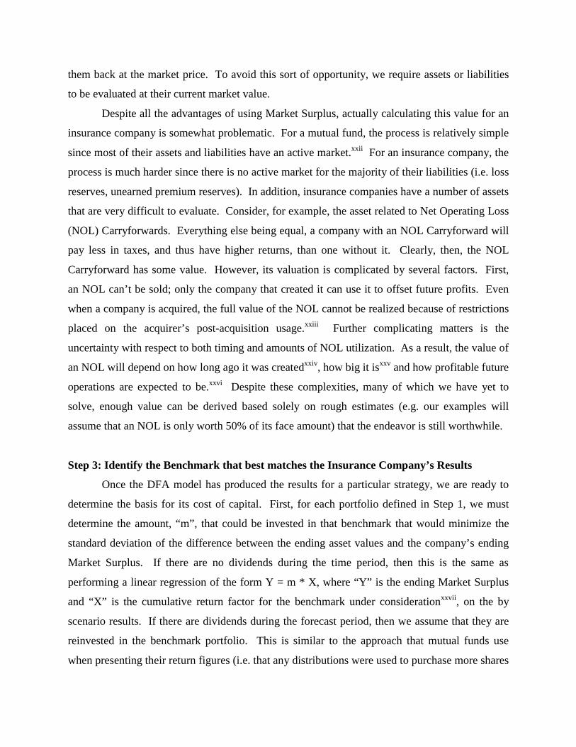
Once the DFA model has produced the results for a particular strategy, we are ready to

determine the basis for its cost of capital. First, for each portfolio defined in Step 1, we must

determine the amount, “m”, that could be invested in that benchmark that would minimize the

standard deviation of the difference between the ending asset values and the company’s ending

Market Surplus. If there are no dividends during the time period, then this is the same as

performing a linear regression of the form Y = m * X, where “Y” is the ending Market Surplus

and “X” is the cumulative return factor for the benchmark under considerationxxvii, on the by

scenario results. If there are dividends during the forecast period, then we assume that they are

reinvested in the benchmark portfolio. This is similar to the approach that mutual funds use

when presenting their return figures (i.e. that any distributions were used to purchase more shares

of the fund), but is more practical for our purposes since it does not involve trying to estimate the

company’s market value at future time periods. Second, we calculate the standard deviation of

the difference at the end of the time period (i.e. the standard deviation of the error term in the

above regression equation). Finally, we select the portfolio that minimizes this standard

deviation. This becomes the basis of the cost of capital for that particular strategy.

To see how this approach works, consider the following simplified example. Table 1

shows the hypothetical cumulative returns for each of four portfolios on the asset-only efficient

frontier. For these same scenarios, we also have the projected ending Market Surplus for a

particular strategy of interest. For the purpose of this example, we have assumed that there are

no intermediate cash flows. Therefore, for each portfolio, we need to determine the amount that

needs to be invested to best duplicate the company’s results (i.e. “m”) through a simple linear

regression. It is important to note that the different portfolios require different amounts of initial

investments. Specifically, the lower expected returns for the benchmark (i.e. Portfolios A and B

in this example) lead to higher initial investment requirements. Once “m” has been determined

for each of the portfolios, we calculate the amount of money this will accumulate to on a

scenario-by-scenario basis (i.e. the “Accumulated Value” figures in the Table). For each

portfolio, we calculate the difference between these results and the company’s projected ending

Market Surplus. Next, we calculate the standard deviation of the by scenario differences.

Finally, we select the portfolio that minimizes the standard deviation of this difference. In this

example, Portfolio C is the benchmark for the strategy of interest.

There are a number of items worth mentioning about this approach. First, in finance

theory, the difference we are considering is referred to as the diversifiable, or non-systematic,

risk. Specifically, it is independent of the returns on all the other securities in the marketplace.

If it weren’t, then we would be able to add or subtract some portion of the correlated asset to

reduce the tracking error, which would violate the way in which the portfolio was selected.

According to finance theory, investors do not need to be compensated for this risk (i.e. it doesn’t

affect their cost of capital) because they will simply diversify it away with the other holdings in

their portfolio. Second, it is important to note that the cost of capital is based on the entire

company’s operations. As a result, we are deriving a basis for the ENTIRE strategy’s cost of

capital even if we are only considering changes to some of the components of that strategy (e.g.

investment strategy). This goes to back to one of the basic tenets of DFA modeling: what

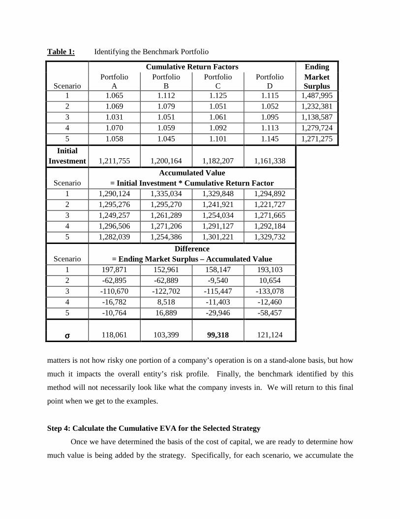
Table 1: Identifying the Benchmark Portfolio

Cumulative Return Factors Ending

Scenario Portfolio

A Portfolio

B Portfolio

C Portfolio

D Market Surplus

1 1.065 1.112 1.125 1.115 1,487,995 2 1.069 1.079 1.051 1.052 1,232,381 3 1.031 1.051 1.061 1.095 1,138,587 4 1.070 1.059 1.092 1.113 1,279,724 5 1.058 1.045 1.101 1.145 1,271,275

Initial Investment 1,211,755 1,200,164 1,182,207 1,161,338

Accumulated Value Scenario = Initial Investment * Cumulative Return Factor

1 1,290,124 1,335,034 1,329,848 1,294,892 2 1,295,276 1,295,270 1,241,921 1,221,727 3 1,249,257 1,261,289 1,254,034 1,271,665 4 1,296,506 1,271,206 1,291,127 1,292,184 5 1,282,039 1,254,386 1,301,221 1,329,732 Difference

Scenario = Ending Market Surplus – Accumulated Value 1 197,871 152,961 158,147 193,103 2 -62,895 -62,889 -9,540 10,654 3 -110,670 -122,702 -115,447 -133,078 4 -16,782 8,518 -11,403 -12,460 5 -10,764 16,889 -29,946 -58,457

σσσσ 118,061 103,399 99,318 121,124

matters is not how risky one portion of a company’s operation is on a stand-alone basis, but how

much it impacts the overall entity’s risk profile. Finally, the benchmark identified by this

method will not necessarily look like what the company invests in. We will return to this final

point when we get to the examples.

Step 4: Calculate the Cumulative EVA for the Selected Strategy

Once we have determined the basis of the cost of capital, we are ready to determine how

much value is being added by the strategy. Specifically, for each scenario, we accumulate the

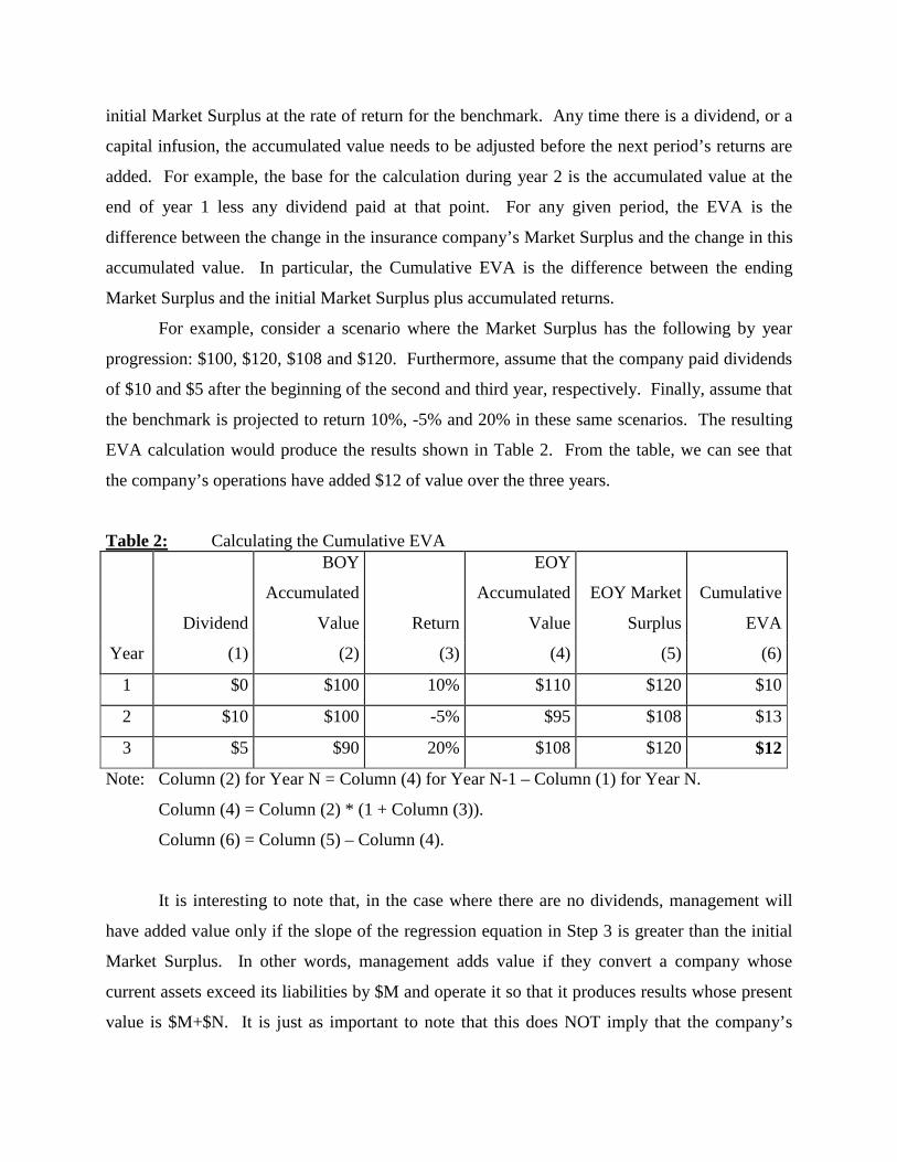
initial Market Surplus at the rate of return for the benchmark. Any time there is a dividend, or a

capital infusion, the accumulated value needs to be adjusted before the next period’s returns are

added. For example, the base for the calculation during year 2 is the accumulated value at the

end of year 1 less any dividend paid at that point. For any given period, the EVA is the

difference between the change in the insurance company’s Market Surplus and the change in this

accumulated value. In particular, the Cumulative EVA is the difference between the ending

Market Surplus and the initial Market Surplus plus accumulated returns.

For example, consider a scenario where the Market Surplus has the following by year

progression: $100, $120, $108 and $120. Furthermore, assume that the company paid dividends

of $10 and $5 after the beginning of the second and third year, respectively. Finally, assume that

the benchmark is projected to return 10%, -5% and 20% in these same scenarios. The resulting

EVA calculation would produce the results shown in Table 2. From the table, we can see that

the company’s operations have added $12 of value over the three years.

Table 2: Calculating the Cumulative EVA

Dividend

BOY

Accumulated

Value Return

EOY

Accumulated

Value

EOY Market

Surplus

Cumulative

EVA

Year (1) (2) (3) (4) (5) (6)

1 $0 $100 10% $110 $120 $10

2 $10 $100 -5% $95 $108 $13

3 $5 $90 20% $108 $120 $12

Note: Column (2) for Year N = Column (4) for Year N-1 – Column (1) for Year N.

Column (4) = Column (2) * (1 + Column (3)).

Column (6) = Column (5) – Column (4).

It is interesting to note that, in the case where there are no dividends, management will

have added value only if the slope of the regression equation in Step 3 is greater than the initial

Market Surplus. In other words, management adds value if they convert a company whose

current assets exceed its liabilities by $M and operate it so that it produces results whose present

value is $M+$N. It is just as important to note that this does NOT imply that the company’s

stock is expected to return more than its cost of capital. Specifically, if the market believes that

the company is going to produce results that are currently worth $M+$N, then the company’s

stock price will be bid up to that level. To the extent that the price is some other value, there

must be a difference between the company’s projections and the investors’ expectations.

Now that we have explained the theory, we will show how it can be applied to an actual

company. We will start with a very simple example to help explain some of the basic features of

the approach.

A Simple Example

Simple Insurance Company has, despite its name, never written a single insurance policy,

nor do they plan to. Currently, they do not pay any income taxes. In fact, their only expenses

are related to managing their investment portfolio. Now, clearly, this is a VERY simplistic

insurance company. In fact, “insurance company” is somewhat of a misnomer: it is actually a

mutual fund. Even so, we can still see some of the dynamics of the proposed approach in this

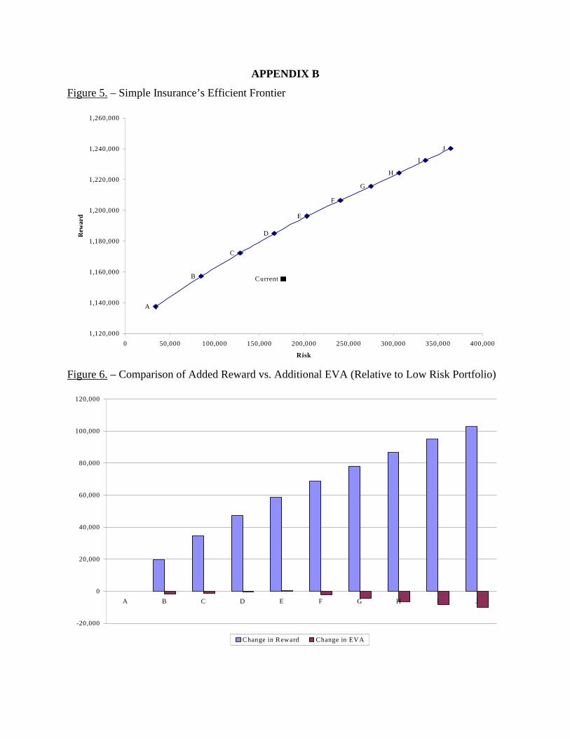
example. Figure 5 shows Simple’s efficient frontier for asset allocation strategies. Clearly,

Simple has some room for improvement. Unfortunately, how they change to reap these benefits

remains somewhat of a mystery. In particular, because the slope of the efficient frontier is fairly

constant, there is no obvious strategy for Simple.

So what about the EVA for each of these strategies? Figure 6 shows the results of the

approach we have described in this paper. Based on this analysis, Simple should move towards

point E, a roughly 50/50 mix of stocks and bonds. Up to that point, the additional return

generated has almost exactly offset the additional risk in the efficient portfolios. Beyond that

point, though, the increased risk starts to dominate the additional reward. As a result, the EVA

trails off. For Simple, the explanation for this result is fairly straightforward: portfolios beyond

E have more equities than Simple does in its current portfolio. Because equities have both

higher annual management fees and higher fees for new purchases, these portfolios trail their

benchmarks by significant amounts.

There are several lessons we should take away from this rudimentary example. First, the

EVA approach has done exactly what we wanted it to: it gave us a single measure that takes into

account both risk and reward. As a result, it can help differentiate between portfolios that might

otherwise be hard to compare, even in this case. Second, one of the problems with this approach

is something that mutual funds have had to deal with for years: the returns on indices do not

reflect any expenses. As a result, it may be unrealistic to hope to exactly match the benchmark’s

return. One way to fix this would be to subtract some reasonable fee from the returns.

Unfortunately, even this seemingly simple solution would be complicated by the fact that what is

“reasonable” depends heavily on the type of investor (e.g. corporations with millions to invest

tend to get much lower fees than individuals with thousands at their disposal). Third, and

perhaps most concerning, it suggests that it is difficult for a company’s asset managers to add

value through superior security selection. In particular, one of our implicit assumptions is that

whatever returns an asset manager can achieve, the investor can get through some other vehicle.

One way to address this problem would be to model different results for the company’s internal

assets and those generally available in the marketplace. Under this approach, an asset manager

who can consistently return 100 basis points more than the S&P without taking on additional risk

would be adding substantial value. Of course, this would require determining how we expect the

two to differ, not at all an easy task. The second approach, and the one we have chosen to adopt,

is to recognize that there are several ways investors can use its asset manager’s expertise. One,

obviously, is to buy the company’s stock. The second is to have a separate mutual fund run by

these same managers. If the asset managers are truly adding substantial value, then the

shareholders would be able to reap more benefit from the mutual fund since the company’s stock

will be impacted by a number of other factors.

A Simple Example – Take 2

Simple Insurance Company, much to the chagrin of their shareholders, has managed to

make themselves subject to US taxation. Clearly, this will dramatically lower their return

potential. Figure 7 shows that this change will cost the company about $100 million over their

three-year projection period in expected reward.xxviii Interestingly, Figure 8 indicates that this

change has slightly increased the slope of the curve, but otherwise has little effect on the tradeoff

between the different strategies.xxix Without the benefit of the EVA analysis, we would probably

be inclined to move out further on the curve because of this slightly better tradeoff. However,

the results for the EVA analysis do not mesh with this intuition (Figure 9). In particular, the

clear winning strategy is now point A, a combination of cash and short-term bonds. The reason

for this, given the previous results when there were no taxes, is that strategy A has the least

amount of taxes because it has the lowest returns. The other interesting fact that this example

demonstrates is that the basis of the cost of capital will not necessarily be the same as the

company’s asset allocation.

To see how this result arises, let us focus on point E, the 50/50 mix of stocks and bonds

that was the optimal solution when there were no taxes. With the introduction of taxes, this

strategy’s benchmark has changed to a 35/65 mix. Because stocks are expected to have higher

returns, this lowers the average cost of capital by about 60 basis points, partially offsetting the

additional tax burdenxxx. But how could this happen? How could adding taxes change the basis

for the strategy’s cost of capital? The first thing to note is that taxes not only reduce the reward,

but also the risk of any particular strategy. In this case, the risk has dropped a little over 35%

(i.e. the standard US Income Tax rate). The reason that it has dropped slightly more than the tax

rate is that the current US tax code does not treat positive and negative results symmetrically. In

particular, taxes on positive results are due immediately. Negative results, on the other hand,

need to be carried forward in the hopes of being used to offset future profits, which makes them

less than their face value. This change has the impact of dropping the skew of the terminal

Market Surplus from 0.595 to 0.496. The net result of this change is that the company’s returns

are more like those of a bond and less like those of equities, which leads to the revision in the

basis for the cost of capital.

DFA Insurance Company (DFAIC)

Having seen the benefit of this approach to some rudimentary examples, we are now

ready to proceed to a more realistic example. DFAIC is a privately held property-casualty

insurance company operating in all fifty states with business concentrations in the northeast and

mid-west. The company writes personal and “main-street” commercial coverage through

independent agents. The company writes business primarily in the northeast and mid-west.xxxi

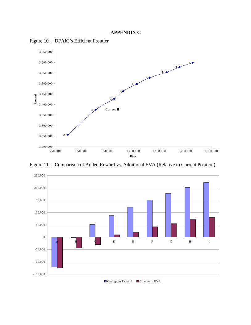
DFAIC is considering changing its investment strategy to try and improve its results. Figure 10

indicates that DFAIC has some limited room for improvement. However, a review of the EVA

for these efficient strategies shows a very clear preference for the higher-reward portfolios. In

particular, this analysis suggests that DFAIC would be best served by moving to point I, a

10/60/30 mix of cash, stocks and bonds, respectively.xxxii Let us take a closer look at how this

happens.

From the Simple Insurance example with taxes, we know that higher-reward portfolios

tend to produce higher corporate income tax burdens. Figure 12 confirms that expectation:

Portfolio I incurs over $200 million more in taxes than the lower returning Portfolio A. Another

obstacle that higher-rewarding strategies pointed out by the EVA approach is that their

associated higher risk leads to an increase in the average costs of capital. For DFAIC, this means

a difference of nearly 2% per year, or roughly $300 million over their five-year planning

horizon, between Portfolios A and I (Figures 13 and 14). Another detriment to riskier strategies

stems from the regulated nature of insurance companies. Specifically, every year insurance

regulators look at a company’s financial health to evaluate its viability. If they feel that the

company is in trouble, they will begin placing restrictions on the company’s operations. Even if

the company manages to recover, the damage to the company’s long-term prospects may not be

reversible.xxxiii While there is no exact method to predict the timing and type of regulatory

intervention, it is still important to allow for its effect, especially when considering very different

strategies. For the purpose of this analysis, we have assumed that the company’s ability to

produce new business is permanently impaired in any scenario where they exceed a 2:1 Premium

to Statutory Surplus ratio at any point during the projection period.xxxiv While reality is likely to

be much more complicated, even this simplistic approach has a significant impact: DFAIC’s

business is hampered in nearly 20% of the scenarios for Portfolio I, as opposed to less than 2%

for Portfolio A. So how is Portfolio I is able to overcome these disadvantages?

The answer lies in the nature of an insurance company. Specifically, insurance

companies write new business in order to leverage their capital. In the case of DFAIC, this

means that a company with only $2.2 billion of Market Surplus controls over $5 billion in

investable assets. As a result of this leverage, Figure 15 indicates that Portfolio I generates over

$700 million more in returns than Portfolio A.xxxv Without that leverage, Portfolio I would not

have been able to generate enough returns to offset its disadvantages, which is what we saw in

the case of Simple Insurance with taxes. It is also important to note that the benefit of this

leverage is also seen in the basis of the cost of capital. Specifically, the benchmark for Portfolio

I is a 70/30 mix of stocks and bonds, as opposed to Simple Insurance where taxes actually

lowered the allocation to stocks.

Conclusion

This paper has presented a new way of comparing different corporate strategies: the

Economic Value Added (EVA). Specifically, by blending together the power of today’s

Dynamic Financial Analysis (DFA) models with the tenets of financial theory, we are able to

determine a benchmark against which the company can compare its results. In particular, by

comparing the growth in the company’s Market Surplus to the returns on this benchmark across

a broad range of scenarios, we are able to arrive at the strategy that maximizes EVA. In so

doing, we ensure that management is performing one of its basic functions: operating the

company in the best interests of their shareholders. Despite the power of this new approach,

there are still several areas that can and should be developed to help improve the theory. In order

to keep the discussion on this important topic moving forward, we will focus on two of the more

important such issues: 1. insurance industry systemic risk and 2. expanding the universe of

portfolios to allow shorting.

As was pointed out in the “Identify the Benchmark…” section, the EVA method

described in this paper is driven largely by an attempt to split a company’s overall risk: systemic

and non-systemic. The reason this split is important is that investors only require additional

returns for taking on systemic risk. Non-systemic risk, on the other hand, doesn’t change the

cost of capital because it can be diversified away. For insurance companies, this is a particularly

difficult question to answer. For example, natural catastrophes are one of the largest single risks

facing many insurance companies. However, there is no reason to believe that these events are

correlated with any other investments. In fact, this is often one of the selling points for the

different methods companies have used to try and sell these risks directly to the capital markets

(e.g. catastrophe bonds, swaps). This brings up the rather unsettling possibility that companies

that focus on highly volatile catastrophe business may actually have a fairly low cost of capital.

One way address this issue is by adding an “insurance industry” index to the available

investment options used to determine the basis of the cost of capital. Clearly, the returns on this

index would need to be correlated with the company’s underwriting results. As a result, to the

extent that such an investment was part of the portfolios on the asset-only efficient frontier, we

would reclassify some of the insurance company’s risks as systemic. If this new asset didn’t

affect the efficient frontier, we would be in a much better position to defend these sorts of

unexpected results.

Another issue that needs to be addressed is whether or not to include the ability to short

(i.e. “sell” an asset today in anticipation of buying it back after its price has dropped) some or all

of the available investments when determining the asset-only efficient frontier. In today’s

increasingly complex capital markets, there are numerous ways for investors to either directly

(e.g. buying on margin) or indirectly (e.g. futures, options, swaps) short any number of different

financial instruments. One issue with allowing these types of investments is that they tend to be

much more expensive than the underlying instruments. Specifically, the counterparty to the

short (i.e. the entity that “buys” the asset) needs to be compensated for the risk that the “seller”

will not be able to deliver the asset should its price go up. Another issue with shorting is that it

invariably leads to scenarios in which the investor suffers a loss greater than his/her initial

investment. If we want to assume that the investor can simply walk away from such situations,

just as they would an insolvent company, then they should be getting charged an option fee at the

beginning of the transaction. If, on the other hand, we assume that such shortfalls will be met

with additional cash flows, we run into the thorny issue of determining the opportunity cost of

this contingent borrowing.

Neither of these issues should be seen as a reason to dismiss this new EVA approach.

Rather, we hope that they will stimulate discussion within the actuarial community about making

this method even more robust. By continuing this discussion, we hope to develop even more

sophisticated tools to aid in the management of insurance companies.

APPENDIX A

Figure 1. – Five Year, Asset-Only Efficient Frontier

Figure 2. – Portfolio Composition of the Efficient Frontier

15%

20%

25%

30%

35%

40%

5% 10% 15% 20% 25% 30% 35% 40%

Standard Deviation

Co

mp

ou

nd

Rea

l R

etu

rn

0%

10%

20%

30%

40%

50%

60%

70%

80%

90%

100%

cash us US Stock Corp 1-5

Corp 5-10 Corp 10-30

Figure 3. – Portfolio Composition of the Five Year, Annualized Total Return Efficient Frontier

Figure 4. – Portfolio Composition of the One Year, Cumulative Real Return Efficient Frontier

0%

10%

20%

30%

40%

50%

60%

70%

80%

90%

100%

cash us US Stock Gov't 1-5 Corp 1-5 Corp 5-10 Corp 10-30 M uni 1-5

0%

10%

20%

30%

40%

50%

60%

70%

80%

90%

100%

cash us US Stock Gov't 1-5

Corp 1-5 Corp 5-10 Corp 10-30

APPENDIX B

Figure 5. – Simple Insurance’s Efficient Frontier

Figure 6. – Comparison of Added Reward vs. Additional EVA (Relative to Low Risk Portfolio)

J

I

H

G

F

E

D

C

B

A

Current

1,120,000

1,140,000

1,160,000

1,180,000

1,200,000

1,220,000

1,240,000

1,260,000

0 50,000 100,000 150,000 200,000 250,000 300,000 350,000 400,000

Risk

Rew

ard

-20,000

0

20,000

40,000

60,000

80,000

100,000

120,000

A B C D E F G H I J

Change in Reward Change in EVA

Figure 7. – Impact of Taxes on Simple Insurance’s Efficient Frontier

Figure 8. – Impact of Taxes on Simple Insurance’s Risk vs. Reward Trade Off

JI

HG

FE

DC

B

A

JIHGF

ED

CB

A

1,000,000

1,050,000

1,100,000

1,150,000

1,200,000

1,250,000

1,300,000

0 50,000 100,000 150,000 200,000 250,000 300,000 350,000 400,000

Risk

Rew

ard

W ithout Taxes W ith Taxes

0%

5%

10%

15%

20%

25%

30%

35%

40%

45%

A to B B to C C to D D to E E to F F to G G to H H to I I to J

Rat

io o

f Cha

nge

in R

ewar

d to

Cha

nge

in R

isk

W ithout Taxes W ith Taxes

Figure 9. – Impact of Taxes on Cumulative EVA

-45,000

-40,000

-35,000

-30,000

-25,000

-20,000

-15,000

-10,000

-5,000

0

5,000

A B C D E F G H I J

Rel

ativ

e EV

A A

dded

W ithout Taxes W ith Taxes

APPENDIX C

Figure 10. – DFAIC’s Efficient Frontier

Figure 11. – Comparison of Added Reward vs. Additional EVA (Relative to Current Position)

IH

G

F

E

D

C

B

A

Current

3,200,000

3,250,000

3,300,000

3,350,000

3,400,000

3,450,000

3,500,000

3,550,000

3,600,000

3,650,000

750,000 850,000 950,000 1,050,000 1,150,000 1,250,000 1,350,000

Risk

Rew

ard

-150,000

-100,000

-50,000

0

50,000

100,000

150,000

200,000

250,000

A B C D E F G H I

Change in Reward Change in EVA

Figure 12. – Additional Taxes Incurred (Relative to Low Risk Position)

Figure 13. –Average Cost of Capital

7.0%

7.5%

8.0%

8.5%

9.0%

9.5%

10.0%

10.5%

A B C D E F G H I

0

50,000

100,000

150,000

200,000

250,000

A B C D E F G H I

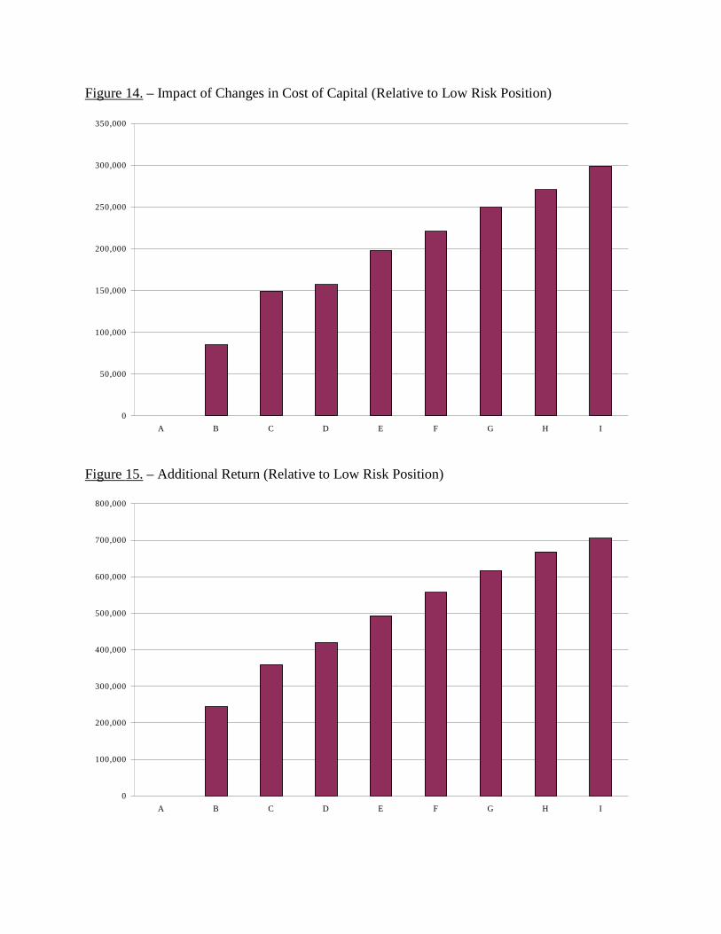
Figure 14. – Impact of Changes in Cost of Capital (Relative to Low Risk Position)

Figure 15. – Additional Return (Relative to Low Risk Position)

0

50,000

100,000

150,000

200,000

250,000

300,000

350,000

A B C D E F G H I

0

100,000

200,000

300,000

400,000

500,000

600,000

700,000

800,000

A B C D E F G H I

REFERENCES

Brazil – A Country Study. Library of Congress, Federal Research Division. 20 February 2001 <http://rs6.loc.gov/frd/cs/brtoc.html>.

Burkett, John, Thomas McIntyre and Stephen M. Sonlin, “DFA Insurance Company Case Study, Part I: Reinsurance and Asset Allocation,” Casualty Actuarial Society Forum, Summer 2001. Arlington, VA: Casualty Actuarial Society.

Correnti, Salvatore, Stephen M. Sonlin and Daniel B. Isaac, “Applying a DFA Model to Improve Strategic Business Decisions,” Casualty Actuarial Society Forum, Summer 1998, 15-51. Arlington, VA: Casualty Actuarial Society.

D’Arcy, Stephen P., Richard W. Gorvett, Thomas E. Hettinger and Robert J. Walling III, “Using the Public Access DFA Model: A Case Study,” Casualty Actuarial Society Forum, Summer 1998, 53-118. Arlington, VA: Casualty Actuarial Society.

Fama, Eugene F. and Kenneth R. French, “The Corporate Cost of Capital and the Return on Corporate Investment,” Journal of Finance, 54(1999): 1939-1967.

Government Bonds. Bloomberg L.P. 20 February 2001 <http://www.bloomberg.com>.

Kaufman, Allan M. and Thomas A. Ryan, “Strategic Asset Allocation for Multi-Line Insurers Using Dynamic Financial Analysis,” Casualty Actuarial Society Forum, Summer 2000, 1-20. Arlington, VA: Casualty Actuarial Society.

Kirschner, Gerald S., “A Cost/Benefit Analysis of Alternative Investment Strategies Using Dynamic Financial Analysis Tools,” Casualty Actuarial Society Forum, Summer 2000, 21-54. Arlington, VA: Casualty Actuarial Society.

Lehman Brothers, Inc., New York, New York. Global Family of Indices, 1998.

Markowitz, Harry M. Portfolio Selection: Efficient Diversification of Investments. 2nd ed. New York: Blackwell, 1991.

Modigliani, Franco and Merton H. Miller, “Corporate Income Taxes and the Cost of Capital: A Correction,” American Economic Review, 1963.

Modigliani, Franco and Merton H. Miller, “The Cost of Capital, Corporation Finance and the Theory of Investment,” American Economic Review, 1958.

Morningstar Quicktake Report - VFICX. Morningstar, Inc. 28 February 2001 <http://quicktake.morningstar.com>.

Morningstar Quicktake Report - VPMCX. Morningstar, Inc. 28 February 2001 <http://quicktake.morningstar.com>.

Philbrick, Stephen and Robert Painter, “DFA Insurance Company Case Study, Part II: Capital Adequacy and Allocation,” Casualty Actuarial Society Forum, Summer 2001. Arlington, VA: Casualty Actuarial Society.

Sec. 382. Limitation on net operating loss carryforwards and certain built-in losses following ownership change. John Walker. Fourmilab Switzerland. 28 February 2001 <http://www.fourmilab.ch>.

The Vanguard Group, Inc. Vanguard Intermediate-Term Corporate Fund’s Prospectus, 9 February 2000.

The Vanguard Group, Inc., Vanguard Primecap Fund’s Prospectus, 7 April 2000.

The Year 2000 in Review. Morningstar, Inc. 20 February 2001 <http://www.morningstar.com>.

END NOTES

i Salvatore Correnti, et. al., “Applying a DFA Model to Improve Strategic Business Decisions” and Stephen P. D’Arcy et. al., “Using the Public Access DFA Model: A Case Study” in the Casualty Actuarial Society Forum, (Arlington, VA: Casualty Actuarial Society, 1998). ii Allan Kaufman and Thomas Ryan, “Strategic Asset Allocation for Multi-Line Insurers Using Dynamic Financial Analysis” and Gerard Kirschner, “A Cost/Benefit Analysis of Alternative Investment Strategies Using Dynamic Financial Analysis Tools” in the Casualty Actuarial Society Forum, (Arlington, VA: Casualty Actuarial Society, 2000). iii It is important to note that the cost of capital will include an implicit component for compensating the company’s shareholders. The cost of financing of a project is usually thought of only in terms of interest rates on debt financing (e.g. bonds, mortgages). iv As of February 20th, 2001, yields on 3-month Japanese Treasury bills were 0.218%. Bloomberg. www.bloomberg.com. v Brazilian inflation peaked at 50% (~ 1.4% per day) during June of 1994. Library of Congress, Federal Research Division. rs6.loc.gov/frd/cs/brtoc.html vi The Vanguard Group, Inc. Vanguard Primecap Fund’s Prospectus, April 7, 2000. p. 24. vii Morningstar. The Year 2000 in Review. www.morningstar.com. viii Vanguard Primecap, 2000, p. 1. ix The S&P 500 is a market weighted index consisting of the stocks of 500 of the largest US based companies whose stocks are frequently traded. x The Vanguard Group, Inc. Vanguard Intermediate-Term Corporate Fund’s Prospectus, February 9, 2001, p. 14. xi The Lehman Brothers Aggregate Bond Index is a market-weighted index of all investment grade debt with 1. at least $100 million outstanding, 2. at least one year to maturity, 3. a fixed rate and 4. US dollar denominated. Global Family of Indices, Lehman Brothers Inc. New York, New York. 1998, p. xxxvii. xii In the rest of this paper, we will use the terms “benchmark” and “basis of the cost of capital” interchangeably. xiii Morningstar.com (www.morningstar.com) reports for Vanguard Primecap (VPMCX) and Intermediate-Term Corporate Bond funds. xiv Lehman Brother’s Municipal Bond Index only includes tax-free debt obligations of states and municipalities in the United States. xv Only the income on municipal bonds is tax-free. Any realized gains would be taxable. xvi The asset-only efficient frontier consists of those investment strategies that maximize reward for each possible level of risk. Unlike the efficient frontiers that are discussed in the DFA literature, this frontier is calculated without reference to a particular insurance company’s operations. xvii Specifically, since tax-free Municipal Bonds should always be priced at a discount to US Treasuries because of their tax advantages, we would expect a portfolio of Treasuries to dominate (i.e. have more reward AND lower risk) than a similarly constructed one of Municipal Bonds. As a result, there shouldn’t be any portfolios on the Efficient Frontier that contain Municipal Bonds. xviii Harry Markowitz, Portfolio Selection: Efficient Diversification of Investments. New York : Blackwell, 1991. xix There is also an adjustment necessary for any items that are contingent on the actual realization of these values (e.g. taxes on unrealized capital gains). xx The market’s value of a company’s future operations can be estimated by comparing the Market Surplus figure we are calculating to the current market value of a company’s outstanding securities. xxi The bond’s return will change only if the bond is sold, retired (e.g. called, converted into shares) or if its NAIC rating category gets lowered. xxii Mutual funds occasionally have to estimate the current market value for certain privately placed instruments and for assets with “stale” prices (i.e. investments that haven’t recently) such as stocks listed on foreign exchanges. xxiii If a company acquires another company with an outstanding NOL, it can only use 10% of its value per year. Section 382, “Limitation on net operating loss carryforwards and certain built-in losses following ownership change” of the U.S. Tax Code. www.fourmilab.ch/ustax/ustax.html. xxiv Older NOLs are more likely to expire worthless and so have less value. xxv The “last” dollar of NOL can only be used after all the previous NOLs have been used, so NOLs have a decreasing marginal value.

xxvi An increase in future profitability will increase the expected speed with which an NOL can be used. This, in turn, will increase its value. xxvii For any given year, the return factor is 1 plus the return for that year. For a multi-period projection, the cumulative return factor is the product of the factors for each year in the projection. xxviii It is important to note that the strategies on the “With Taxes” curve are the same as the corresponding strategies on the “Without Taxes” Efficient Frontier. As a result, they may or may not be on the “With Taxes” Efficient Frontier, but the two curves are directly comparable. xxix We are specifically NOT considering what would be the most logical course of action for Simple at this point: liquidating and returning the proceeds to the shareholders. xxx The impact on a scenario by scenario basis is much more pronounced: the cost of capital was lower by as much as 18% in certain scenarios and higher in others by as much as 8% for within the 1000 scenarios we modeled. While this has very little impact on the Cumulative EVA, since it is based on averages, it will dramatically impact any historical analysis management might perform. xxxi For a more detailed description of DFAIC, please refer to John Burkett, et. al., “DFA Insurance Company Case Study, Part I: Reinsurance and Asset Allocation” and Stephen Philbrick and Robert Painter, “DFA Insurance Company Case Study, Part II: Capital Adequacy and Allocation” in the Casualty Actuarial Society Forum, (Arlington, VA: Casualty Actuarial Society, 2001). xxxii DFAIC’s asset allocation strategy required at least 10% cash (actually, one-month T-Bills) and no more than 60% stocks. xxxiii Rating agencies can have a similar effect on a company’s operations when results deteriorate. Specifically, rating agencies can either suggest restrictions (e.g. buying more reinsurance) that are necessary to maintain a current rating or it can lower the company’s rating, which will likely impact the company’s ability to sell its products. xxxiv DFAIC is currently writing at about 1.45:1. xxxv This amount includes additional returns off DFAIC’s future cash flows, since they get invested once DFAIC generates them, as well as those off the initial $5 billion.