better-than-chance classi cation for signal detection · 2017-12-15 · better-than-chance classi...

Better-Than-Chance Classification for SignalDetection

Jonathan D. RosenblattDepartment of IE&M and

Zlotowsky Center for Neuroscience,Ben Gurion University of the Negev, Israel.

Yuval BenjaminiDepartment of Statistics,Hebrew University, Israel

Roee GilronMovement Disorders and Neuromodulation Center,

University of California, San Francisco.

Roy MukamelSchool of Psychological Science

Tel Aviv University, Israel.

Jelle GoemanDepartment of Medical Statistics and Bioinformatics,Leiden University Medical Center, The Netherlands.

December 15, 2017

AbstractThe estimated accuracy of a classifier is a random quantity with

variability. A common practice in supervised machine learning, is thusto test if the estimated accuracy is significantly better than chancelevel. This method of signal detection is particularly popular in neu-roimaging and genetics. We provide evidence that using a classifier’saccuracy as a test statistic can be an underpowered strategy for find-ing differences between populations, compared to a bona-fide statisti-cal test. It is also computationally more demanding than a statistical

1

arX

iv:1

608.

0887

3v2

[st

at.M

E]

14

Dec

201

7

Classification for Signal Detection 1 INTRODUCTION

test. Via simulation, we compare test statistics that are based on clas-sification accuracy, to others based on multivariate test statistics. Wefind that probability of detecting differences between two distributionsis lower for accuracy based statistics. We examine several candidatecauses for the low power of accuracy tests. These causes include: thediscrete nature of the accuracy test statistic, the type of signal accu-racy tests are designed to detect, their inefficient use of the data, andtheir regularization. When the purposes of the analysis is not signaldetection, but rather, the evaluation of a particular classifier, we sug-gest several improvements to increase power. In particular, to replaceV-fold cross validation with the Leave-One-Out Bootstrap.

Keywords: signal-detection; multivariate-testing; supervised-learning;hypothesis-testing; high-dimension

1 Introduction

Many neuroscientists and geneticists detect signal by fitting a classifier andtesting whether it’s prediction accuracy is better than chance. The workflowconsists of fitting a classifier, and estimating its predictive accuracy usingcross validation. Given that the cross validated accuracy is a random quan-tity, it is then common to test if the cross validated accuracy is significantlybetter than chance using a permutation test. Examples in the neuroscientificliterature include Golland and Fischl [2003], Pereira et al. [2009], Schreiberand Krekelberg [2013], Varoquaux et al. [2016], and especially the recentlypopularized multivariate pattern analysis (MVPA) framework of Kriegesko-rte et al. [2006]. For examples in the genetics literature see for example Golubet al. [1999], Slonim et al. [2000], Radmacher et al. [2002], Mukherjee et al.[2003], Juan and Iba [2004], Jiang et al. [2008].

To fix ideas, we will adhere to a concrete example. In Gilron et al. [2016],the authors seek to detect brain regions that encode differences betweenvocal and non-vocal stimuli. Following the MVPA workflow, the localizationproblem is cast as a supervised learning problem: if the type of the stimuluscan be predicted from the brain’s activation pattern significantly better thanchance, then a region is declared to encode vocal/non-vocal information. Wecall this an accuracy test, because it uses the prediction accuracy as a teststatistic.

This same signal detection task can also be approached as a multivariatetest. Inferring that a region encodes vocal/non-vocal information, is essen-tially inferring that the spatial distribution of brain activations is differentgiven a vocal/non-vocal stimulus. As put in Pereira et al. [2009]:

2


... the problem of deciding whether the classifier learned to dis-criminate the classes can be subsumed into the more general ques-tion as to whether there is evidence that the underlying distribu-tions of each class are equal or not.

A practitioner may thus approach the signal detection problem with a two-group location test such as Hotelling’s T 2 [Anderson, 2003]. Alternatively, ifthe size of the brain’s region of interest is large compared to the number ofobservations, so that the spatial covariance cannot be fully estimated, thena high dimensional version of Hotelling’s test can be called upon. Examplesof high dimensional multivariate tests include Schafer and Strimmer [2005],Goeman et al. [2006], or Srivastava [2007] . For brevity, and in contrastto accuracy tests, we will call these location tests, because they test for theequality of location of two multivariate distributions.

At this point, it becomes unclear which is preferable: a location testor an accuracy test? The former with a heritage dating back to Hotelling[1931], and the latter being extremely popular, as the 1, 170 citations1 ofKriegeskorte et al. [2006] suggest.

The comparison between location and accuracy tests was precisely thegoal of Ramdas et al. [2016], who compared Hotelling’s T 2 location test toFisher’s linear discriminant analysis (LDA) accuracy test. By comparing therates of convergence of the power of each statistic, Ramdas et al. [2016] con-cluded that accuracy and location tests are rate equivalent. Rates, however,are only a first stage when comparing test statistics.

Asymptotic relative efficiency measures (ARE) are typically used by statis-ticians to compare between rate-equivalent test statistics [van der Vaart,1998]. ARE is the limiting ratio of the sample sizes required by two statis-tics to achieve similar power. Ramdas et al. [2016] derive the asymptoticpower functions of the two test statistics, which allows to compute the AREbetween Hotelling’s T 2 (location) test and Fisher’s LDA (accuracy) test.Theorem 14.7 of van der Vaart [1998] relates asymptotic power functions toARE. Using this theorem and the results of Ramdas et al. [2016] we deducethat the ARE is lower bounded by 2π ≈ 6.3. This means that Fisher’s LDArequires at least 6.3 more samples to achieve the same (asymptotic) power asthe T 2 test. In this light, the accuracy test is remarkably inefficient comparedto the location test. For comparison, the t-test is only 1.04 more (asymptot-ically) efficient than Wilcoxon’s rank-sum test [Lehmann, 2009], so that anARE of 6.3 is strong evidence in favor of the location test.

Before discarding accuracy tests as inefficient, we recall that Ramdaset al. [2016] analyzed a half-sample holdout. The authors conjectured that a

1GoogleScholar. Accessed Aug 2017.

3


leave-one-out approach, which makes more efficient use of the data, may havebetter performance. Also, the analysis in Ramdas et al. [2016] is asymptotic.This eschews the discrete nature of the accuracy statistic, which we willshow to have crucial impact. Since typical sample sizes in neuroscience arenot large, we seek to study which test is to be preferred in finite samples,and not only asymptotically. Our conclusion will be quite simple: locationtests typically have more power than accuracy tests, are easier to implement,and interpret.

Our statement rests upon the observation that with typical sample sizes,the accuracy test statistic is highly discrete. Permutation testing with dis-crete test statistics are known to be conservative [Hemerik and Goeman,2017], since they are insensitive to mild perturbations of the data, and can-not exhaust the permissible false positive rate. As put by Prof. Frank Harrellin CrossValidated2 post back in 2011:

... your use of proportion classified correctly as your accuracyscore. This is a discontinuous improper scoring rule that can beeasily manipulated because it is arbitrary and insensitive.

The degree of discretization is governed by the number of samples. Inour example from Gilron et al. [2016], the classification accuracy is computedusing 40 samples, so that the test statistic may assume only 40 possiblevalues. This number of samples is not unusual in an neuroimaging study.

Power loss due to discretization is further aggravated if the test statistic ishighly concentrated. For an intuition consider the usage of the resubstitutionaccuracy, a.k.a. the train error, or empirical risk, as a test statistic. Resub-stitution accuracy is the accuracy of the classifier evaluated on the trainingset. If data is high dimensional, the resubstitution accuracy will be very highdue to over fitting. In a very high dimensional regime, the resubstitution ac-curacy may be as high as 1 for the observed data [McLachlan, 1976, Theorem1], but also for any permutation. The concentration of resubstitution accu-racy near 1, and its discretization, render this test completely useless, withpower tending to 0 for any (fixed) effect size, as the dimension of the modelgrows.

To compare the power of accuracy tests and location tests in finite sam-ples, we study a battery of test statistics by means of simulation. We startwith formalizing the problem in Section 2. The main findings are reportedin Sections 3, and 4. A discussion follows.

2A Q&A website for statistical questions: http://stats.stackexchange.com/

questions/17408/how-to-assess-statistical-significance-of-the-accuracy-of-a-classifier

4

http://stats.stackexchange.com/questions/17408/how-to-assess-statistical-significance-of-the-accuracy-of-a-classifier

http://stats.stackexchange.com/questions/17408/how-to-assess-statistical-significance-of-the-accuracy-of-a-classifier

Classification for Signal Detection 2 PROBLEM SETUP

2 Problem setup

2.1 Multivariate Testing

Let y ∈ Y be a class encoding. Let x ∈ X be a p dimensional feature vector.In our vocal/non-vocal example we have Y = {0, 1} and p = 27, the numberof voxels in a brain region so that X = R27.

Denoting a dataset by S := {(xi, yi)}ni=1, a multivariate test amounts totesting whether the distribution of x given y = 1 is the same as x given y = 0.For example, we can test whether multivariate voxel activation patterns (x)are similarly distributed when given a vocal stimulus (y = 1) or a non-vocalone (y = 0). The tests are calibrated to have a fixed false positive rate(α = 0.05). The comparison metric between statistics is power, i.e., theprobability to infer that x|y = 1 is not distributed like x|y = 0.

2.2 From a Test Statistic to a Permutation Test

The multivariate tests we will be considering rely on fixing some test statistic,and comparing it to it’s permutation distribution. The tests differ in thestatistic they employ. Our comparison metric is their power, i.e., their truepositive rate. We adhere to permutation tests and not parametric inferencebecause our problems of interest are typically high-dimensional. This meansthat n � p does not hold, and central limit laws do not apply. Becausewe focus on two-group testing under an independent sampling assumption,we know that a label-switching permutation test is valid even if possiblyconservative. The sketch of our permutation test is the following:(a) Fix a test statistic T with a right tailed rejection region.(b) Sample a random permutation of the class labels, π(y).(c) Permute labels and recompute the statistic Tπ.(d) Repeat (a)-(c) R times.(e) The permutation p-value is the proportion of Tπ larger than the observedT . Formally: P{Tπ ≥ T } := 1

R

∑π I{Tπ ≥ T }.

(f) Declare classes differ if the permutation p-value is smaller than α, whichwe set to α = 0.05.

We now detail the various test statistics that will be compared.

2.3 Location Tests and Hotelling’s T 2

The most prevalent interpretation of “x|y = 1 is not distributed like x|y = 0”is to assume they differ in means. In his seminal work, Hotelling [1931] has

5


proposed the T 2 test statistic for testing the equality in means of two mul-tivariate distributions. Using our notations this statistic is proportional tothe difference between group means, measured with the Mahalanobis norm:

T 2 ∝ (xy=1 − xy=0)′ Σ−1 (xy=1 − xy=0), (1)

where xy=j is the p-vector of means in the y = j group, and Σ is a pooledcovariance estimator. Perhaps more intuitively, T 2 is Euclidean norm of themean difference vector, but after transforming to decorrelated scales. Formore background see, for example, Anderson [2003].

The major difficulty with these multivariate tests is that Σ has p(p+1)/2free parameters, so that n has to be very large to apply these tests. If nis not much larger than p, or in low signal-to-noise (SNR), the test is verylow powered, as shown by Bai and Saranadasa [1996]. In these cases, highdimensional versions of the T 2 should be applied, which essentially regularizethe estimator of Σ, thus reducing the dimensionality of the problem andimproving the SNR and power.

2.4 Prediction Accuracy as a Test Statistic

An accuracy test amounts to using a predictor’s accuracy as a test statistic.A predictor3, AS : X → Y , is the output of a learning algorithm A

when applied to the dataset S. The accuracy of predictor4, EAS , is definedas the probability of AS making a correct prediction. The accuracy of analgorithm5, EA, is defined as the expected accuracy over all possible data setsS. Formalizing, we denote by P the probability measure of (x, y), and by PSthe joint probability measure of the sample S. We can then write

EAS :=

∫(x,y)

I{AS(x) = y} dP , (2)

and

EA :=

∫SEAS dPS , (3)

where I{A} is the indicator function6 of the set A.Denoting an estimate of EAS by EAS , and EA by EA, a statistically signifi-

cant “better than chance” estimate of either, is evidence that the classes aredistinct.

3Known as a hypothesis in the machine learning literature.4Known as (the complement of) the test error in Friedman et al. [2001]5Known as (the complement of) the expected test error in Friedman et al. [2001]6Mutatis mutandis for continous y.

6


Two popular estimates of EA are the resubstitution estimate, and theV-fold Cross Validation (CV) estimate.

Definition 1 (Resubstitution estimate). The resubstitution accuracy esti-mator of a learning algorithm A, denoted EResubA , is defined as

EResubA :=1

n

n∑i=1

I{AS(xi) = yi}. (4)

Definition 2 (V-fold CV estimate). Denoting by Sv the v’th partition, orfold, of the dataset, and by S(v) its complement, so that Sv∪S(v) = ∪Vv=1Sv =S, the V-fold CV accuracy estimator, denoted EV foldA , is defined as

EV foldA :=1

V

V∑v=1

1

|Sv|∑i∈SvI{AS(v)(xi) = yi}, (5)

where |A| denotes the cardinality of a set A.

2.5 How to Estimate Accuracies?

Estimating EA requires the following design choices: Should it be cross-validated and how? If cross validating using V-fold CV then how many folds?Should the folding be balanced? If estimation is part of a permutation test:should the data be refolded after each permutation?

We will now address these questions while bearing in mind that unlikethe typical supervised learning setup, we are not interested in an unbiasedestimate of EA, but rather in the detection of its departure from chance level.

Cross validate or not? For the purpose of statistical testing, bias in EA isnot a problem, as long as it does not invalidate the error rate guarantees. Theunderlying intuition is that if the same bias is introduced in all permutations,it will not affect the properties of the permutation test. We will thus beconsidering both cross validated accuracies, and resubstitution accuracies.

Balanced folding? The standard practice in V-fold CV is to constrain thedata folds to be balanced, i.e. stratified [e.g. Ojala and Garriga, 2010]. Thismeans that each fold has the same number of examples from each class. Wewill report results with both balanced and unbalanced data foldings.

7


Refolding? In V-fold CV, folding the data means assigning each observa-tion to one of the V data folds. The standard practice in neuroimaging isto permute labels and refold the data after each permutation. This is donebecause permuting labels will unbalance the original balanced folding. Wewill adhere to this practice due to its popularity, even though it is compu-tationally more efficient to permute features7 instead of labels, as done byGolland et al. [2005].

How many folds? Different authors suggest different rules for the numberof folds. We fix the number of folds to V = 4, and do dot discuss the effectof V because we will ultimately show that V-fold CV is dominated by othercross-validation procedures, and thus, never recommended.

Table 1 collects an initial battery of tests we will be comparing.

Name Algorithm Resampling Parameters

Oracle Hotelling Resubstitution –Hotelling Hotelling Resubstitution –Hotelling.shrink Hotelling Resubstitution –Goeman Hotelling Resubstitution –sd Hotelling Resubstitution –lda.CV.1 LDA V-fold –lda.noCV.1 LDA Resubstitution –svm.CV.1 SVM V-fold cost=10svm.CV.2 SVM V-fold cost=0.1svm.noCV.1 SVM Resubstitution cost=10svm.noCV.2 SVM Resubstitution cost=0.1

Table 1: This table collects the various test statistics we will be studying. Lo-cation tests include: Oracle, Hotelling, Hotelling.shrink, Goeman, and sd. Oracleis the same as Hotelling’s T 2, only using the generative covariance, and not anestimated one. Hotelling is the classical two-group T 2 statistic [Anderson, 2003].Hotelling.shrink is a high dimensional version of T 2, with the regularized covari-ance from Schafer and Strimmer [2005]. Goeman and sd are other high dimensionalversions of the T 2, from Goeman et al. [2006] and Srivastava [2013]. The rest of thetests are accuracy tests, with details given in the table. For example, svm.CV.2 isa linear SVM, with V-fold cross validated accuracy, and cost parameter set at 0.1[Meyer et al., 2015]. Another example is lda.noCV.1, which is Fisher’s LDA, witha resubstituted accuracy estimate.

7The difference between permuting labels or features is in the mapping to folds. Whenpermuting features, the label assignment to folds is fixed. When permuting labels, thefeature assignment to folds is fixed.

8

Classification for Signal Detection 3 RESULTS

3 Results

We now compare the power of our various statistics in various configurations.We do so via simulation. The basic simulation setup is presented in Sec-tion 3.1. Following sections present variations on the basic setup. The R codefor the simulations can be found in http://www.john-ros.com/permuting_

accuracy/.

3.1 Basic Simulation Setup

Each simulation is based on 1, 000 replications. In each replication, we gen-erate n i.i.d. samples from a shift class

xi = µyi + ηi, (6)

where yi ∈ Y = {0, 1} encodes the class of subject i, µ is a p-dimensionalshift vector, the noise ηi is distributed as Np (0,Σ), the sample size n = 40,and the dimension of the data is p = 23. The covariance Σ = I. In thisbasic setup, reported in Figure 1, the shift effect is captured by µ. Shiftsare equal in all p coordinates of µ. With e being a p-vector of ones, thenµ := c e. We will use c to index the signal’s strength, and vary it overc ∈ {0, 1/4, 1/2}. The (squared) Euclidean and Mahalanobis norms of thesignal are ‖µ‖2

2 = ‖µ‖2Σ = c2p ≈ {0, 1.4, 5.7}. These can be thought as the

effect’s size.Having generated the data, we compute each of the test statistics in Ta-

ble 1. For test statistics that require data folding, we used 4 folds. Wethen compute a permutation p-value by permuting the class labels, and re-computing each test statistic. We perform 300 such permutations. We thenreject the “x|y = 0 distributed like x|y = 1” null hypothesis if the permuta-tion p-value is smaller than 0.05. The reported power is the proportion ofreplication where the permutation p-value fell below 0.05.

3.2 False Positive Rate

We start with a sanity check. Theory suggests that all test statistics shouldcontrol their false positive rate. Our simulations confirm this. In all ourresults, such as Figure 1, we encode the null case, where no signal is presentand x|y = 1 has the same distribution as x|y = 0, by a red circle. Sincethe red circles are always below the desired 0.05 error rate then the falsepositive rate of all test statistics, in all simulations is controlled. We maythus proceed and compare the power of each test statistic.

9

http://www.john-ros.com/permuting_accuracy/

http://www.john-ros.com/permuting_accuracy/


3.3 Power

Having established that all of the tests in our battery control the false pos-itive rate, it remains to be seen if they have similar power– especially whencomparing location tests to accuracy tests.

From Figure 1 we learn that location tests are more powerful than accu-racy tests. This is particularly visible for intermediate signal strength (greentriangle), and location tests Goeman, sd and Hotelling.shrink defined in Ta-ble 1.

Figure 1: The power of the permutation test with various test statistics. The poweron the x axis. Effects are color and shape coded. The various statistics on the y axis.Their details are given in Table 1. Effects vary over c = 0 (red circle), c = 1/4 (greentriangle), and c = 1/2 (blue square). Simulation details in Section 3.1. Cross-validationwas performed with balanced and unbalanced data folding; see sub-captions.

●

●

●

●

●

●

●

●

●

●

●

Oracle

Hotelling

Hotelling.shrink

Goeman

sd

lda.CV.1

lda.noCV.1

svm.CV.1

svm.CV.2

svm.noCV.1

svm.noCV.2

0.00 0.25 0.50 0.75 1.00

Power

(a) Unbalanced V-fold CV.

●

●

●

●

●

●

●

●

●

●

●

Oracle

Hotelling

Hotelling.shrink

Goeman

sd

lda.CV.1

lda.noCV.1

svm.CV.1

svm.CV.2

svm.noCV.1

svm.noCV.2

0.00 0.25 0.50 0.75 1.00

Power

(b) Balanced V-fold CV.

3.4 Tie Breaking

As already stated in the introduction, the accuracy statistic is highly dis-crete. Especially the resubstitution accuracy tests. Discrete test statisticslose power by not exhausting the permissible false positive rate. A commonremedy is a randomized test, in which the rejection of the null is decided atrandom in a manner that exhausts the false positive rate. Formally, denotingby T the observed test statistic, by Tπ, its value after under permutation π,and by P{A} the proportion of permutations satisfying A then the random-ized version of our tests imply that if the permutation p-value, P{Tπ ≥ T },

10


is greater than α then we reject the null with probability

max

{α− P{Tπ > T }P{Tπ = T }

, 0

}.

Figure 2 reports the same analysis as in Figure 1b, after allowing for ran-dom tie breaking. It demonstrates that the power disadvantage of accuracytests, cannot be remedied by random tie breaking.

●

●

●

●

●

●

●

●

●

●

●

Oracle

Hotelling

Hotelling.shrink

Goeman

sd

lda.CV.1

lda.noCV.1

svm.CV.1

svm.CV.2

svm.noCV.1

svm.noCV.2

0.00 0.25 0.50 0.75 1.00

Power

Figure 2: The same as Figure 1b, with random tie breaking.

3.5 Departure From Gaussianity

The Neyman-Pearson Lemma (NPL) type reasoning that favors the locationtest over accuracy tests may fail when the data is not multivariate Gaussian,and Hotelling’s T 2 statistic no longer a generalized-likelihood-ratio test.

To check this, we replaced the multivariate Gaussian distribution of η inEq.(6) with a heavy-tailed multivariate-t distribution. In this heavytailedsetup, the dominance of the location tests was preserved, even if less evidentthan in the Gaussian case (Figure 3).

3.6 Departure from Sphericity

We now test the robustness of our results to the correlations in x. In termsof Eq.(6), Σ will no longer be the identity matrix. Intuitively- both locationtests and accuracy tests include the estimation of Σ, so that correlations

11


●

●

●

●

●

●

●

●

●

●

●

Oracle

Hotelling

Hotelling.shrink

Goeman

sd

lda.CV.1

lda.noCV.1

svm.CV.1

svm.CV.2

svm.noCV.1

svm.noCV.2

0.0 0.2 0.4 0.6 0.8

Power

Figure 3: Heavytailed. ηi is p-variate t, with df = 3 .

should be accounted for. To keep the comparisons “fair” as the correlationsvary, we kept ‖µ‖Σ :=

√µ′Σ−1µ fixed.

Which test has more power: accuracy or location? We address this ques-tion using various correlation structures. We also vary the direction of thesignal, µ, and distinguish between signal in high variance principal compo-nent (PC) of Σ, and in the low variance PC.

The simulation results reveal some non trivial phenomena. First, whenthe signal is in the direction of the high variance PC, the high dimensionallocation tests are far superior than accuracy tests. This holds true for variouscorrelation structures: the short memory correlations of AR(1) in Figure 4a,the long memory correlations of a Brownian motion in Figure 5a, and thearbitrary correlation in Figure 6a.

When the signal is in the direction of the low variance PC, a differentphenomenon appears. There is no clear preference between location or ac-curacy tests. Instead the non-regularized tests are the clear victors. Thisholds true for various correlation structures: the short memory correlationsof AR(1) in Figure 4b, the long memory correlations of a Brownian motionin Figure 5b, and the arbitrary correlation in Figure 6b. We attribute thisphenomenon to the bias introduced by the regularization, which masks thesignal. This matter is further discussed in Section 5.3.

12


Figure 4: Short memory, AR(1) correlation. Σk,l = ρ|k−l|; ρ = 0.6

●

●

●

●

●

●

●

●

●

●

●

Oracle

Hotelling

Hotelling.shrink

Goeman

sd

lda.CV.1

lda.noCV.1

svm.CV.1

svm.CV.2

svm.noCV.1

svm.noCV.2

0.00 0.25 0.50 0.75 1.00

Power

(a) Signal in direction ofhighest variance PC ofΣ.

●

●

●

●

●

●

●

●

●

●

●

Oracle

Hotelling

Hotelling.shrink

Goeman

sd

lda.CV.1

lda.noCV.1

svm.CV.1

svm.CV.2

svm.noCV.1

svm.noCV.2

0.00 0.25 0.50 0.75 1.00

Power

(b) Signal in direction oflowest variance PC ofΣ.

3.7 Departure from Homoskedasticity

Our previous simulations assume variables a have unit variance. The het-eroskedastic case, where difference coordinates have different variance, is oflesser importance, since we can typically normalize the variable-wise variance.Some test statistics have built-in variance normalization, and are known asscalar invariant. The sd test statistic is scalar invariant. Statistics that arenot scalar-invariant such as the Goeman statistic, will give less importanceto high-variance directions than to low-variance directions.

In Figure 7a we see that as before, location tests dominate accuracy tests.For the first time, we can see the difference between the scalar-invariant sdand Goeman: the latter gaining power by focusing on low variance coordi-nates. Since the signal’s magnitude is the same in all coordinates, Goemangains power by putting emphasis where it is needed.

When the signal is in the low variance PC, Goeman puts emphasis onvariables which carry little signal. For this reason it has less power than sd,as seen in Figure 7b.

3.8 Departure from V-fold CV

Intuition suggests we may alleviate the discretization of the accuracy teststatistic by replacing the V-fold CV, and resampling with replacement. Thediscretization of the accuracy statistic is governed by the number of samplesin the union of test sets. For V-fold CV, for instance, the accuracy may

13


Figure 5: Long-memory Brownian motion correlation: Σ = D−1RD−1 where D isdiagonal with Djj =

√Rjj , and Rk,l = min{k, l}.

●

●

●

●

●

●

●

●

●

●

●

Oracle

Hotelling

Hotelling.shrink

Goeman

sd

lda.CV.1

lda.noCV.1

svm.CV.1

svm.CV.2

svm.noCV.1

svm.noCV.2

0.00 0.25 0.50 0.75 1.00

Power


●

●

●

●

●

●

●

●

●

●

●

Oracle

Hotelling

Hotelling.shrink

Goeman

sd

lda.CV.1

lda.noCV.1

svm.CV.1

svm.CV.2

svm.noCV.1

svm.noCV.2

0.00 0.25 0.50 0.75 1.00

Power

(b) Signal in direction oflowest lowest variancePC of Σ.

assume as many values as the sample size. This suggests that the accuracycan be “smoothed” by allowing the test sample to be drawn with replacement.An algorithm that samples test sets with replacement is the leave-one-outbootstrap estimator, and its derivatives, such as the 0.632 bootstrap, and0.632+ bootstrap [Friedman et al., 2001, Sec 7.11].

Definition 3 (bLOO). The leave-one-out bootstrap estimate, bLOO, is theaverage accuracy of the holdout observations, over all bootstrap samples.Denote by Sb, a bootstrap sample b of size n, sampled with replacementfrom S. Also denote by C(i) the index set of bootstrap samples not containingobservation i. The leave-one-out bootstrap estimate, EbLOOA , is defined as:

EbLOOA :=1

n

n∑i=1

1

|C(i)|∑b∈C(i)

I{ASb(xi) = yi}. (7)

An equivalent formulation, which stresses the Bootstrap nature of the algo-rithm is the following. Denoting by S(b) the indexes of observations that arenot in the bootstrap sample b and are not empty,

EbLOOA =1

B

B∑b=1

1

|S(b)|∑i∈S(b)

I{ASb(xi) = yi}. (8)

Simulation results are reported in Figure 8 with naming conventions inTable 2. As expected, selecting test sets with replacement does increase the

14


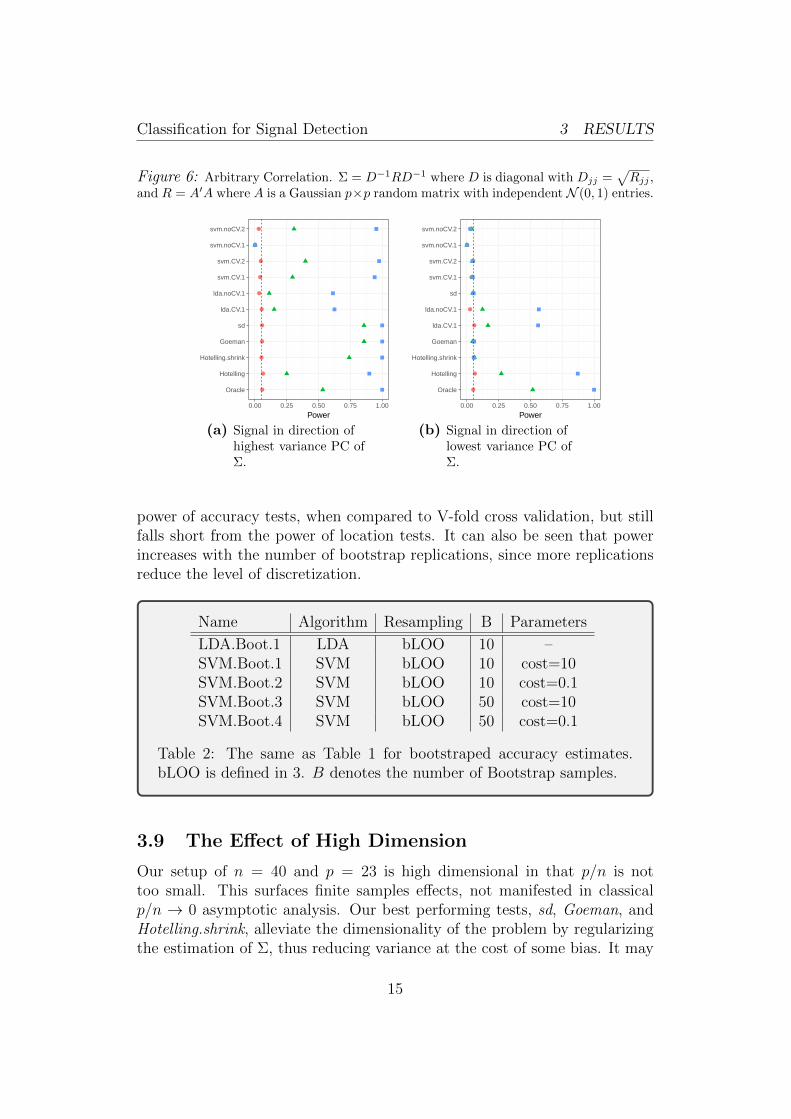
Figure 6: Arbitrary Correlation. Σ = D−1RD−1 where D is diagonal with Djj =√Rjj ,

and R = A′A where A is a Gaussian p×p random matrix with independent N (0, 1) entries.

●

●

●

●

●

●

●

●

●

●

●

Oracle

Hotelling

Hotelling.shrink

Goeman

sd

lda.CV.1

lda.noCV.1

svm.CV.1

svm.CV.2

svm.noCV.1

svm.noCV.2

0.00 0.25 0.50 0.75 1.00

Power


●

●

●

●

●

●

●

●

●

●

●

Oracle

Hotelling

Hotelling.shrink

Goeman

lda.CV.1

lda.noCV.1

sd

svm.CV.1

svm.CV.2

svm.noCV.1

svm.noCV.2

0.00 0.25 0.50 0.75 1.00

Power

(b) Signal in direction oflowest variance PC ofΣ.

power of accuracy tests, when compared to V-fold cross validation, but stillfalls short from the power of location tests. It can also be seen that powerincreases with the number of bootstrap replications, since more replicationsreduce the level of discretization.

Name Algorithm Resampling B Parameters

LDA.Boot.1 LDA bLOO 10 –SVM.Boot.1 SVM bLOO 10 cost=10SVM.Boot.2 SVM bLOO 10 cost=0.1SVM.Boot.3 SVM bLOO 50 cost=10SVM.Boot.4 SVM bLOO 50 cost=0.1

Table 2: The same as Table 1 for bootstraped accuracy estimates.bLOO is defined in 3. B denotes the number of Bootstrap samples.

3.9 The Effect of High Dimension

Our setup of n = 40 and p = 23 is high dimensional in that p/n is nottoo small. This surfaces finite samples effects, not manifested in classicalp/n → 0 asymptotic analysis. Our best performing tests, sd, Goeman, andHotelling.shrink, alleviate the dimensionality of the problem by regularizingthe estimation of Σ, thus reducing variance at the cost of some bias. It may

15


Figure 7: Heteroskedasticity: Σ is diagonal with Σjj = j.

●

●

●

●

●

●

●

●

●

●

●

Oracle

Hotelling

Hotelling.shrink

Goeman

sd

lda.CV.1

lda.noCV.1

svm.CV.1

svm.CV.2

svm.noCV.1

svm.noCV.2

0.00 0.25 0.50 0.75 1.00

Power

(a) µ in the high variancePC of Σ.

●

●

●

●

●

●

●

●

●

●

●

Oracle

Hotelling

Hotelling.shrink

Goeman

sd

lda.CV.1

lda.noCV.1

svm.CV.1

svm.CV.2

svm.noCV.1

svm.noCV.2

0.00 0.25 0.50 0.75 1.00

Power

(b) µ in the low variancePC of Σ.

thus be argued that the power advantages of the location tests are driven bythe regularization of the covariance, and not the statistic itself. We wouldthus augment the comparison with various covariance-regularized accuracytests. The l2 regularization in our SVM accuracy test, already regularizesthe covariance, but it is certainly not the only way to do so. We thus addsome covariance-regularized accuracy tests such as a shrinkage based LDA[Pang et al., 2009, Ramey et al., 2016], where similarly to Hotteling.shrink,Tikhonov regularization of Σ is employed. We also try we try a diagonalizedLDA8 [Dudoit et al., 2002], which regularizes Σ similarly to sd and Goeman.

Simulation results are reported in Figure 9 with naming conventions inTable 3. The proper regularization of the covariance of a classifier, just likea location test, can improve power. See, for instance, svm.CV.6 which isclearly the best regularized SVM for testing. Replacing the V-fold with abootstrap allows us to further increase the power, as done with lda.highdim.4.Even so, the out-of-the-box location tests outperform the accuracy tests.

8Known as Gaussian Naıve Bayes.

16


●

●

●

●

●

●

●

●

●

●

●

●

●

●

●

●

Oracle

Hotelling

Hotelling.shrink

Goeman

sd

lda.CV.1

lda.noCV.1

svm.CV.1

svm.CV.2

svm.noCV.1

svm.noCV.2

svm.Boot.1

svm.Boot.2

svm.Boot.3

svm.Boot.4

lda.Boot.1

0.00 0.25 0.50 0.75 1.00

Power

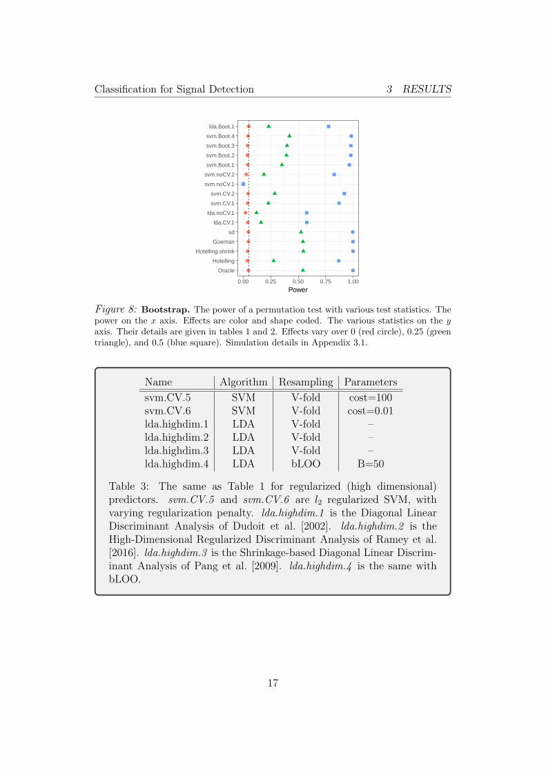
Figure 8: Bootstrap. The power of a permutation test with various test statistics. Thepower on the x axis. Effects are color and shape coded. The various statistics on the yaxis. Their details are given in tables 1 and 2. Effects vary over 0 (red circle), 0.25 (greentriangle), and 0.5 (blue square). Simulation details in Appendix 3.1.

Name Algorithm Resampling Parameters

svm.CV.5 SVM V-fold cost=100svm.CV.6 SVM V-fold cost=0.01lda.highdim.1 LDA V-fold –lda.highdim.2 LDA V-fold –lda.highdim.3 LDA V-fold –lda.highdim.4 LDA bLOO B=50

Table 3: The same as Table 1 for regularized (high dimensional)predictors. svm.CV.5 and svm.CV.6 are l2 regularized SVM, withvarying regularization penalty. lda.highdim.1 is the Diagonal LinearDiscriminant Analysis of Dudoit et al. [2002]. lda.highdim.2 is theHigh-Dimensional Regularized Discriminant Analysis of Ramey et al.[2016]. lda.highdim.3 is the Shrinkage-based Diagonal Linear Discrim-inant Analysis of Pang et al. [2009]. lda.highdim.4 is the same withbLOO.

17

Classification for Signal Detection 4 NEUROIMAGING EXAMPLE

●

●

●

●

●

●

●

●

●

●

●

●

●

●

●

●

Oracle

Hotelling

Hotelling.shrink

Goeman

sd

lda.CV.1

svm.CV.1

svm.CV.2

svm.CV.5

svm.CV.6

lda.highdim.1

lda.highdim.2

lda.highdim.3

lda.highdim.4

svm.Boot.3

svm.Boot.4

0.00 0.25 0.50 0.75 1.00

Power

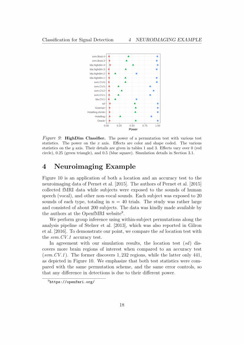
Figure 9: HighDim Classifier. The power of a permutation test with various teststatistics. The power on the x axis. Effects are color and shape coded. The variousstatistics on the y axis. Their details are given in tables 1 and 3. Effects vary over 0 (redcircle), 0.25 (green triangle), and 0.5 (blue square). Simulation details in Section 3.1.

4 Neuroimaging Example

Figure 10 is an application of both a location and an accuracy test to theneuroimaging data of Pernet et al. [2015]. The authors of Pernet et al. [2015]collected fMRI data while subjects were exposed to the sounds of humanspeech (vocal), and other non-vocal sounds. Each subject was exposed to 20sounds of each type, totaling in n = 40 trials. The study was rather largeand consisted of about 200 subjects. The data was kindly made available bythe authors at the OpenfMRI website9.

We perform group inference using within-subject permutations along theanalysis pipeline of Stelzer et al. [2013], which was also reported in Gilronet al. [2016]. To demonstrate our point, we compare the sd location test withthe svm.CV.1 accuracy test.

In agreement with our simulation results, the location test (sd) dis-covers more brain regions of interest when compared to an accuracy test(svm.CV.1 ). The former discovers 1, 232 regions, while the latter only 441,as depicted in Figure 10. We emphasize that both test statistics were com-pared with the same permutation scheme, and the same error controls, sothat any difference in detections is due to their different power.

9https://openfmri.org/

18

https://openfmri.org/

Classification for Signal Detection 5 DISCUSSION

Figure 10: Brain regions encoding information discriminating between vocal and non-vocal stimuli. Map reports the centers of 27-voxel sized spherical regions, as discoveredby an accuracy test (svm.CV.1 ), and a location test (sd). svm.CV.1 was computed using5-fold cross validation, and a cost parameter of 1. Region-wise significance was determinedusing the permutation scheme of Stelzer et al. [2013], followed by region-wise FDR ≤ 0.05control using the Benjamini-Hochberg procedure [Benjamini and Hochberg, 1995]. Numberof permutations equals 400. The location test detect 1, 232 regions, and the accuracy test441, 399 of which are common to both. For the details of the analysis see Gilron et al.[2016].

5 Discussion

We have set out to understand which of the tests is more powerful: accuracytests or location tests. Our current observation is that accuracy tests arenever optimal. There is always a multivariate test, possibly a location test,that dominates in power. Our advice to the practitioner is that locationtests, in particular their regularized versions, are good performers in a widerange of simulation setups and empirically. They are also typically easierto implement, and faster to run, since no resampling is required. Theirhigh-dimensional versions, such as Schafer and Strimmer [2005], Goemanet al. [2006], and Srivastava [2007], are particularly well suited for empiricalproblems such as neuroimaging and genetics.

5.1 Where do Accuracy Tests Lose Power?

The low power of the accuracy tests compared to location tests can be at-tributed to the following causes:(a) Discretization: The discrete nature of accuracy test statistics. Thedegree of discretization is governed by the sample size. For this reason, anasymptotic analysis such as Ramdas et al. [2016], or Golland et al. [2005],

19


will not capture power loss due to discretization10. An asymptotic analysismay suggest resubstitution accuracy estimates are good test statistics, whilethey suffer from very low finite-sample power. The canonical remedy forties— random tie breaking — showed only a minor improvement (Sec. 3.4).(b) Shift Alternatives: We focused on shift alternative so that locationtests are expectedly superior via an NPL type argument.(c) Inefficient use of the data when validating with a holdout set.(d) Inappropriate regularization in high SNR regimes: testing requires lessregularization than predicting.

Given the above reasons and based on our professional experience, wedare argue that an accuracy test will rarely have more power than a high-dimensional location test.

5.2 Interpretation

Multivariate tests, and location tests in particular, are easier to interpret. Todo so we typically use a NPL type argument, and think: What type of signalis a test sensitive to? What is the direction of the effect? etc. Accuracy testsare seen as “black boxes”, even though they can be analyzed in the same way.Gilron et al. [2017] demonstrate that the type of signal captured by accuracytests is less interpretable to neuroimaging practitioners than location tests.

Some authors prefer accuracy tests because they can be seen as effect-sizeestimates, invariant to the sample size. This is true, but the multivariate-statistics literature provides many multivariate effect-size estimators, thatgeneralize Cohen’s d, and do not suffer from discretization like accuracy esti-mates. Examples can be found, for instance, in Stevens [2012] and referencestherein.

5.3 Fixed SNR

For a fair comparison between simulations, in particular between those withdifferent Σ, we needed to fix the difficulty of the problem. We defined “afair comparison” to be such that a maximal power test would have the samepower, justifying our choice of fixing the Mahalanobis norm of µ. Formally,in all our simulations we set ‖µ‖2

Σ = c2p.Our choice implies that the Euclidean norm of µ varies with the covari-

ance, and with the direction of the signal. An initial intuition may suggest

10This actually holds for all power analyses relying on a contiguity argument [van derVaart, 1998, Ch.6].

20


that detecting signal in the low variance PCs is easier than in the high vari-ance PCs. This is true when fixing ‖µ‖2, but not when fixing ‖µ‖Σ.

For completeness, Figure 11 reports the power analysis under AR(1) cor-relations, but with ‖µ‖2 fixed instead of ‖µ‖Σ. We compare the power of ashift in the direction of some high variance PC (Figure 11a), versus a shiftin the direction of a low variance PC (Figure 11b). The intuition that itis easier to detect signal in the low variance directions is confirmed. It isalso consistent with Figure 4, in the following aspects: (i)Hotelling.shrink isa good performed “on average”, (ii) sd and Goeman have the best powerto detect signal in the noisiest directions, but low power for signal in thenoiseless directions.

Figure 11: Short memory, AR(1) correlation. ‖µ‖2 fixed.

●

●

●

●

●

●

●

●

●

●

●

Oracle

Hotelling

Hotelling.shrink

Goeman

sd

lda.CV.1

lda.noCV.1

svm.CV.1

svm.CV.2

svm.noCV.1

svm.noCV.2

0.00 0.25 0.50 0.75 1.00

Power

(a) µ in PC7 of Σ.

●

●

●

●

●

●

●

●

●

●

●

Oracle

Hotelling

Hotelling.shrink

Goeman

sd

lda.CV.1

lda.noCV.1

svm.CV.1

svm.CV.2

svm.noCV.1

svm.noCV.2

0.00 0.25 0.50 0.75 1.00

Power

(b) µ in PC15 of Σ.

5.4 Detecting Signal in Different Directions

Figures 4, 5, 6 and 11, demonstrate that detecting signal in the direction ofthe high variance PCs is very different than detecting in the low variancePCs. Why is that?

We attribute this phenomenon to regularization. While the signal, µvaries in direction, the regularization of Σ does not. The various regulariza-tion methods deflate the high variance directions, thus, relatively inflate thelow variance directions. If the signal is in the low variance directions, theregularization may mask it. This is what we see in figures 4b, 5b, and 6b:the unregularized tests have more power than the regularized.

21


5.5 Implications to Other Problems

Our work studies signal detection in the two-group multivariate testing frame-work, i.e., MANOVA framework. The same problem can be cast in theunivariate generalized linear models framework, and in particular, as a Bre-noulli Regression problem. If any of the predictors, x, carries any signal,then x|y = 0 has a different distribution than x|y = 1. This view is the oneadopted Goeman et al. [2006].

Another related problem is that of multinomial-regression, i.e., multi-classclassification. We conjecture that power differences in favor of location testsversus accuracy tests will increase as the number of classes increases.

5.6 Testing in Augmented Spaces

It may be argued that only accuracy tests permits the separation betweenclasses in augmented spaces, such as in reproducing kernel Hilbert spaces(RKHS) by using non-linear predictors. This is a false argument— accu-racy tests do not have any more flexibility than location tests. Indeed, it ispossible to test for location in the same space the classifier is learned. Forindependence tests with kernels see for example Szekely and Rizzo [2009] orGretton et al. [2012].

5.7 A Good Accuracy Test

Brain-computer interfaces and clinical diagnostics [e.g. Olivetti et al., 2012,Wager et al., 2013] are examples where we want to know not only if infor-mation is encoded in a region, but rather, that a particular predictor canextract it. In these cases an accuracy test cannot be replaced by a location,or other, statistical test. For the cases an accuracy test cannot be replacedwith other tests, we collect the following observations.

Sample size. The conservativeness of accuracy tests, due to discretization,decrease with sample size.

Regularize. Regularization proves crucial to detection power in low SNRregimes, such as when n is in the order of p, or under strong correlations. Wefind that the Shrinkage-based Diagonal Linear Discriminant Analysis of Panget al. [2009] is a particularly good performer, but more research is requiredon this matter. Particularly, in the possibility of regularizing in directionsorthogonal to µ.

22


Smooth accuracy. Smooth accuracy estimate by cross validating withreplacement. The bLOO estimator, in particular, is preferable over V-fold.

Resubstitution accuracy in high SNR. Resubstitution accuracy is use-ful in high SNR regimes, such as n � p, because it avoids cross validationwithout compromising power. In low SNR, the power loss is considerable.We attribute this to the compounding of discretization and concentration ef-fects: the difference between the sampling distribution of the resubstitutionaccuracy is simply indistinguishable under the null and under the alternative.In high SNR, the concentration is less impactful, and the computational bur-den of cross validation can be avoided by using the resubstitution accuracy.

5.8 Related Literature

We now review some related accuracy-testing literature, with an emphasison neuroimaging applications. Ojala and Garriga [2010] study the power oftwo accuracy tests differing in their permutation scheme: One testing the “nosignal” null hypothesis, and the other testing the “independent features” nullhypothesis. They perform an asymptotic analysis, and a simulation study.They also apply various classifiers to various data sets. Their emphasis isthe effect of the underlying classifier on the power, and the potential of the“independent features” test for feature selection. This is a very differentemphasis from our own.

Olivetti et al. [2012] and Olivetti et al. [2014] looked into the problemof choosing a good accuracy test. They propose a new test they call anindependence test, and demonstrate by simulation that it has more powerthan other accuracy tests, and can deal with non-balanced data sets. Wedid not include this test in the battery we compared, but we note that theindependence test of Olivetti et al. [2012] relies on a discrete test statistic.It may thus be improved by regularizing and resampling with replacement.

Schreiber and Krekelberg [2013] used null simulations to study the statis-tical properties of linear SVM’s for signal detection, and in particular, falsepositive rates. They did not study the matter of power. They recommendedto test the significance of accuracy estimates using permutation testing in-stead of parametric t-tests, or binomial tests. They recommend so due tothe correlations between data folds in V-fold CV. The authors were also con-cerned with temporal correlations, which biases accuracy estimates even ifcross validated. Bias in accuracy estimates is of great concern when study-ing a classifier, but it is of lesser concern when using the accuracy merely forlocalization. Their recommendations differ from ours: they recommend to

23


ensure independent data foldings in V-fold CV, whereas we claim discretiza-tion is the real concern, and thus recommend bLOO.

Golland and Fischl [2003] and Golland et al. [2005] study accuracy testsusing simulation, neuroimaging data, genetic data, and analytically. Thefinite Vapnik–Chervonenkis dimension requirement [Golland et al., 2005, Sec4.3] implies a the problem is low dimensional and prevents the permutationp-value from (asymptotically) concentrating near 1. They find that the powerincreases with the size of the test set. This is seen in Fig.4 of Golland et al.[2005], where the size of the test-set, K, governs the discretization. Weattribute this to the reduced discretization of the accuracy statistic.

Golland et al. [2005] simulate the power of accuracy tests by samplingfrom a Gaussian mixture family of models, and not from a location familyas our own simulations. Under their model (with some abuse of notation)

(xi|yi = 1) ∼ πN (µ1, I) + (1− π)N (µ2, I) ,

(xi|yi = 0) ∼ (1− π)N (µ1, I) + πN (µ2, I) .

Varying π interpolates between the null distribution (π = 0.5) and a locationshift model (π = 0). We now perform the same simulation as Golland et al.[2005], and in the same dimensionality as our previous simulations. We re-parameterize so that π = 0 corresponds to the null model:

(xi|yi = 1) ∼ (1/2− π)N (µ1, I) + (1/2 + π)N (µ2, I) ,

(xi|yi = 0) ∼ (1/2 + π)N (µ1, I) + (1/2− π)N (µ2, I) .(9)

From Figure 12, we see that also for the mixture class of Golland et al.[2005] locations tests are to be preferred over accuracy tests.

5.9 Epilogue

Given all the above, we find the popularity of accuracy tests for signal de-tection quite puzzling. We believe this is due to a reversal of the inferencecascade. Researchers first fit a classifier, and then ask if the classes are anydifferent. Were they to start by asking if classes are any different, and onlythen try to classify, then location tests would naturally arise as the preferredmethod. As put by Ramdas et al. [2016]:

The recent popularity of machine learning has resulted in the ex-tensive teaching and use of prediction in theoretical and appliedcommunities and the relative lack of awareness or popularity ofthe topic of Neyman-Pearson style hypothesis testing in the com-puter science and related “data science” communities.

24


●

●

●

●

●

●

●

●

●

●

●

Oracle

Hotelling

Hotelling.shrink

Goeman

sd

lda.CV.1

lda.noCV.1

svm.CV.1

svm.CV.2

svm.noCV.1

svm.noCV.2

0.00 0.25 0.50 0.75 1.00

Power

Figure 12: Mixture Alternatives. xi is distributed as in Eq.(9). µ is a p-vector with3/√p in all coordinates. The effect, π, is color and shape coded and varies over 0 (red

circle), 1/4 (green triangle) and 1/2 (blue square).

Acknowledgments

JDR was supported by the ISF 900/60 research grant. JDR also wishes tothank, Jesse B.A. Hemerik, Yakir Brechenko, Omer Shamir, Joshua Vogel-stein, Gilles Blanchard, and Jason Stein for their valuable inputs.

25

Classification for Signal Detection REFERENCES

References

T. W. Anderson. An Introduction to Multivariate Statistical Analysis. Wiley-Interscience, Hoboken, NJ, 3 edition edition, July 2003. ISBN 978-0-471-36091-9.

Z. Bai and H. Saranadasa. Effect of high dimension: by an example of a twosample problem. Statistica Sinica, pages 311–329, 1996.

Y. Benjamini and Y. Hochberg. Controlling the false discovery rate: a prac-tical and powerful approach to multiple testing. JOURNAL-ROYAL STA-TISTICAL SOCIETY SERIES B, 57:289–289, 1995.

S. Dudoit, J. Fridlyand, and T. P. Speed. Comparison of DiscriminationMethods for the Classification of Tumors Using Gene Expression Data.Journal of the American Statistical Association, 97(457):77–87, Mar. 2002.ISSN 0162-1459. doi: 10.1198/016214502753479248.

J. Friedman, T. Hastie, and R. Tibshirani. The elements of statistical learn-ing, volume 1. Springer series in statistics New York, 2001.

R. Gilron, J. Rosenblatt, O. Koyejo, R. A. Poldrack, and R. Mukamel. Quan-tifying spatial pattern similarity in multivariate analysis using functionalanisotropy. arXiv:1605.03482 [q-bio], May 2016.

R. Gilron, J. Rosenblatt, O. Koyejo, R. A. Poldrack, and R. Mukamel. What’sin a pattern? examining the type of signal multivariate analysis uncoversat the group level. NeuroImage, 146:113–120, 2017.

J. J. Goeman, S. A. Van De Geer, and H. C. Van Houwelingen. Testingagainst a high dimensional alternative. Journal of the Royal StatisticalSociety: Series B (Statistical Methodology), 68(3):477–493, 2006.

P. Golland and B. Fischl. Permutation tests for classification: towards statis-tical significance in image-based studies. In IPMI, volume 3, pages 330–341.Springer, 2003.

P. Golland, F. Liang, S. Mukherjee, and D. Panchenko. Permutation Tests forClassification. In P. Auer and R. Meir, editors, Learning Theory, number3559 in Lecture Notes in Computer Science, pages 501–515. Springer BerlinHeidelberg, June 2005. ISBN 978-3-540-26556-6 978-3-540-31892-7. doi:10.1007/11503415 34.

26


T. R. Golub, D. K. Slonim, P. Tamayo, C. Huard, M. Gaasenbeek, J. P.Mesirov, H. Coller, M. L. Loh, J. R. Downing, M. A. Caligiuri, C. D.Bloomfield, and E. S. Lander. Molecular Classification of Cancer: ClassDiscovery and Class Prediction by Gene Expression Monitoring. Science,286(5439):531–537, Oct. 1999. ISSN 0036-8075, 1095-9203. doi: 10.1126/science.286.5439.531.

A. Gretton, K. M. Borgwardt, M. J. Rasch, B. Scholkopf, and A. Smola. AKernel Two-sample Test. J. Mach. Learn. Res., 13:723–773, Mar. 2012.ISSN 1532-4435.

J. Hemerik and J. Goeman. Exact testing with random permutations. TEST,Nov 2017. ISSN 1863-8260. doi: 10.1007/s11749-017-0571-1. URL https:

//doi.org/10.1007/s11749-017-0571-1.

H. Hotelling. The Generalization of Student’s Ratio. The Annals of Math-ematical Statistics, 2(3):360–378, Aug. 1931. ISSN 0003-4851, 2168-8990.doi: 10.1214/aoms/1177732979.

W. Jiang, S. Varma, and R. Simon. Calculating confidence intervals forprediction error in microarray classification using resampling. StatisticalApplications in Genetics and Molecular Biology, 7(1), 2008.

L. Juan and H. Iba. Prediction of tumor outcome based on gene expressiondata. Wuhan University Journal of Natural Sciences, 9(2):177–182, Mar.2004. ISSN 1007-1202, 1993-4998. doi: 10.1007/BF02830598.

N. Kriegeskorte, R. Goebel, and P. Bandettini. Information-based functionalbrain mapping. Proceedings of the National Academy of Sciences of theUnited States of America, 103(10):3863–3868, July 2006. ISSN 0027-8424,1091-6490. doi: 10.1073/pnas.0600244103.

E. L. Lehmann. Parametric versus nonparametrics: two alternative method-ologies. Journal of Nonparametric Statistics, 21(4):397–405, 2009. ISSN1048-5252. doi: 10.1080/10485250902842727.

G. J. McLachlan. The bias of the apparent error rate in discriminant analysis.Biometrika, 63(2):239–244, Jan. 1976. ISSN 0006-3444, 1464-3510. doi:10.1093/biomet/63.2.239.

D. Meyer, E. Dimitriadou, K. Hornik, A. Weingessel, and F. Leisch. e1071:Misc Functions of the Department of Statistics, Probability Theory Group(Formerly: E1071), TU Wien. 2015. R package version 1.6-7.

27

https://doi.org/10.1007/s11749-017-0571-1

https://doi.org/10.1007/s11749-017-0571-1


S. Mukherjee, P. Tamayo, S. Rogers, R. Rifkin, A. Engle, C. Campbell,T. R. Golub, and J. P. Mesirov. Estimating dataset size requirementsfor classifying DNA microarray data. Journal of Computational Biology:A Journal of Computational Molecular Cell Biology, 10(2):119–142, 2003.ISSN 1066-5277. doi: 10.1089/106652703321825928.

M. Ojala and G. C. Garriga. Permutation Tests for Studying Classifier Perfor-mance. Journal of Machine Learning Research, 11(Jun):1833–1863, 2010.ISSN ISSN 1533-7928.

E. Olivetti, S. Greiner, and P. Avesani. Induction in Neuroscience withClassification: Issues and Solutions. In G. Langs, I. Rish, M. Grosse-Wentrup, and B. Murphy, editors, Machine Learning and Interpretationin Neuroimaging, number 7263 in Lecture Notes in Computer Science,pages 42–50. Springer Berlin Heidelberg, 2012. ISBN 978-3-642-34712-2978-3-642-34713-9. doi: 10.1007/978-3-642-34713-9 6.

E. Olivetti, S. Greiner, and P. Avesani. Statistical independence for theevaluation of classifier-based diagnosis. Brain Informatics, 2(1):13–19, Dec.2014. ISSN 2198-4018, 2198-4026. doi: 10.1007/s40708-014-0007-6.

H. Pang, T. Tong, and H. Zhao. Shrinkage-based Diagonal DiscriminantAnalysis and Its Applications in High-Dimensional Data. Biometrics, 65(4):1021–1029, Dec. 2009. ISSN 1541-0420. doi: 10.1111/j.1541-0420.2009.01200.x.

F. Pereira, T. Mitchell, and M. Botvinick. Machine learning classifiers andfMRI: A tutorial overview. NeuroImage, 45(1, Supplement 1):S199–S209,Mar. 2009. ISSN 1053-8119. doi: 10.1016/j.neuroimage.2008.11.007.

C. R. Pernet, P. McAleer, M. Latinus, K. J. Gorgolewski, I. Charest, P. E. G.Bestelmeyer, R. H. Watson, D. Fleming, F. Crabbe, M. Valdes-Sosa, andP. Belin. The human voice areas: Spatial organization and inter-individualvariability in temporal and extra-temporal cortices. NeuroImage, 119:164–174, Oct. 2015. ISSN 1053-8119. doi: 10.1016/j.neuroimage.2015.06.050.

M. D. Radmacher, L. M. McShane, and R. Simon. A Paradigm forClass Prediction Using Gene Expression Profiles. Journal of Computa-tional Biology, 9(3):505–511, June 2002. ISSN 1066-5277. doi: 10.1089/106652702760138592.

A. Ramdas, A. Singh, and L. Wasserman. Classification Accuracy as a Proxyfor Two Sample Testing. arXiv:1602.02210 [cs, math, stat], Feb. 2016.

28


J. A. Ramey, C. K. Stein, P. D. Young, and D. M. Young. High-DimensionalRegularized Discriminant Analysis. arXiv preprint arXiv:1602.01182,2016.

J. Schafer and K. Strimmer. A Shrinkage Approach to Large-Scale CovarianceMatrix Estimation and Implications for Functional Genomics. StatisticalApplications in Genetics and Molecular Biology, 4(1), Jan. 2005. ISSN1544-6115. doi: 10.2202/1544-6115.1175.

K. Schreiber and B. Krekelberg. The statistical analysis of multi-voxel pat-terns in functional imaging. PLoS One, 8(7):e69328, 2013.

D. K. Slonim, P. Tamayo, J. P. Mesirov, T. R. Golub, and E. S. Lander. ClassPrediction and Discovery Using Gene Expression Data. In Proceedings ofthe Fourth Annual International Conference on Computational MolecularBiology, RECOMB ’00, pages 263–272, New York, NY, USA, 2000. ACM.ISBN 978-1-58113-186-4. doi: 10.1145/332306.332564.

M. S. Srivastava. Multivariate Theory for Analyzing High Dimensional Data.Journal of the Japan Statistical Society, 37(1):53–86, 2007. doi: 10.14490/jjss.37.53.

M. S. Srivastava. On testing the equality of mean vectors in high dimension.Acta et Commentationes Universitatis Tartuensis de Mathematica, 17(1):31–56, June 2013. ISSN 2228-4699. doi: 10.12697/ACUTM.2013.17.03.

J. Stelzer, Y. Chen, and R. Turner. Statistical inference and multiple test-ing correction in classification-based multi-voxel pattern analysis (MVPA):Random permutations and cluster size control. NeuroImage, 65:69–82, Jan.2013. ISSN 1053-8119. doi: 10.1016/j.neuroimage.2012.09.063.

J. P. Stevens. Applied multivariate statistics for the social sciences. Rout-ledge, 2012.

G. J. Szekely and M. L. Rizzo. Brownian distance covariance. The Annals ofApplied Statistics, 3(4):1236–1265, Dec. 2009. ISSN 1932-6157, 1941-7330.doi: 10.1214/09-AOAS312.

A. W. van der Vaart. Asymptotic Statistics. Cambridge University Press,Cambridge, UK ; New York, NY, USA, Oct. 1998. ISBN 978-0-521-49603-2.

G. Varoquaux, P. R. Raamana, D. Engemann, A. Hoyos-Idrobo, Y. Schwartz,and B. Thirion. Assessing and tuning brain decoders: cross-validation,caveats, and guidelines. working paper or preprint, June 2016.

29


T. D. Wager, L. Y. Atlas, M. A. Lindquist, M. Roy, C.-W. Woo, and E. Kross.An fMRI-Based Neurologic Signature of Physical Pain. New England Jour-nal of Medicine, 368(15):1388–1397, Apr. 2013. ISSN 0028-4793. doi:10.1056/NEJMoa1204471.

30

better-than-chance classi cation for signal detection · 2017-12-15 · better-than-chance classi...

Documents