Better Statistics, Better Economic Policies?*

Johannes Binswanger� Manuel Oechslin�

September 28, 2020

Abstract

More and more economic transactions leave a “digital footprint”. This trend opens

unprecedented opportunities for improving economic statistics and underpins demands to

give statistical agencies far-reaching access to private-sector data. We analyze the conse-

quences of better economic statistics in a political-agency framework that includes funda-

mental uncertainty about the impact of potentially welfare-enhancing reforms. We demon-

strate that improvements in economic statistics can inhibit—rather than stimulate—

reform attempts. With better statistics, the government is less likely to receive the “benefit

of the doubt” if the numbers suggest its past reforms are failing. Reforms therefore come

with a higher risk of electoral losses, implying that the government has stronger incen-

tives to preserve the status quo. We identify political environments that are particularly

vulnerable to this mechanism and contribute to the debate on private-sector data access.

Keywords: Digitalization, economic statistics, political economy, reforms, uncertainty

*We thank seminar and conference participants at Goethe University Frankfurt, Harvard University Kennedy

School of Government, UC Louvain, University of Geneva, University of Gothenburg, University of Lucerne,

the 2017 Annual Conference of the Society for Institutional & Organizational Economics in New York, and the

2018 Annual Conference of the Royal Economic Society in Brighton for helpful comments. An earlier version

of this paper circulated under the title “Smaller Measurement Errors, Better Economic Policies?”.�University of St. Gallen, School of Economics and Political Science, Department of Economics, Bodanstrasse

8, CH-9000 St.Gallen, Switzerland; e-mail: johannes.binswanger@unisg.ch.�Corresponding author. University of Lucerne, Department of Economics, P.O. Box 4466, CH-6002 Lucerne,

Switzerland; e-mail: manuel.oechslin@unilu.ch. CentER, Tilburg University, The Netherlands.

1

1 Introduction

In recent years, the amount of data available in digital form has been expanding fast (see, e.g.,

National Academies, 2017). An ever-growing number of devices generate data on people and

businesses. More and more economic transactions automatically leave a “digital footprint”.

These developments promise unprecedented opportunities for statistical offices in charge of key

economic indicators such as GDP growth, inflation, and job creation (see, e.g., Coyle, 2014;

Karabell, 2014; Jarmin, 2019). Sample frames can be broadened and data access accelerated

at low cost. Proxy indices, useful inputs into estimations when timely survey data is missing,

can be made more informative. More generally, “big data” offers opportunities to broaden the

set of economic indicators with a view to specific evaluation tasks. To take advantage of these

opportunities, statistical agencies around the world demand statutory changes that would give

them the legal right to regularly access large amounts of private-sector data. The European

Statistical System (2017, p. 2), for instance, suggested that the European Commission come

up “with relevant provisions that would establish a general principle of access to privately-held

data which are of public interest.”1 The extent to which democratic societies should accede to

such demands is among the key policy questions of our time. The present paper contributes

to the current debate from a political-economy perspective.

Currently, official economic statistics suffer from several limitations. For one, economists

have documented that GDP estimates are often imprecise and subject to large revisions (e.g.,

Croushore, 2011; Manski, 2015). As a result, policy makers and business leaders face sig-

nificant uncertainty when consulting the latest estimates to gauge whether the economy has

been gaining or losing momentum recently. At the same time, economists increasingly mind

that the results of reforms and new programs are often context-specific and therefore hard to

predict with accuracy (Manski, 2013).2 So there is a rising interest in concepts such as growth

diagnostics (Rodrik, 2010) and experimentation at scale (Muralidharan and Niehaus, 2017),

i.e., approaches that emphasize “[policy] experimentation as a strategy for discovery of what

works, along with monitoring and evaluation.” (Rodrik, 2010, p. 41). With these concepts in

mind, improvements in the precision and breadth of economic statistics are highly welcome:

evaluation processes become more informative, thereby speeding up the learning process about

what “works”. In fact, improving the evaluations of reforms and new programs is an important

argument in the statistical agencies’ quest for new data sources.

1The UK Statistics Authority (2016) made a similar suggestion, which found its way into the Digital EconomyAct of 2017. See Bostic et al. (2016) and Jarmin (2019, p. 177) for the state of the discussion in the US.

2Muralidharan and Niehaus (2017, p. 103) note that “[governments] often roll out new government programsrepresenting millions (...) of dollars of expenditure with little evidence to indicate whether they will work.”

2

It is an obvious conclusion that better economic statistics are unambiguously helpful if

politicians are guided by the common interest and pursue a “dashboard approach” to eco-

nomic policy. In this paper, we ask whether this conclusion will continue to hold if politicians

are self-interested and subject to a common choice distortion. The answer is no. Paradoxically,

better economic statistics may weaken, rather than strengthen, politicians’ incentives to initi-

ate promising reforms if the reforms’ optimal design is subject to substantial uncertainty and

must be discovered in an experimental fashion. To grasp intuitively why progress in economic

statistics may “backfire”, note that ambiguities and uncertainties in economic statistics often

play a prominent role in the public discourse on policy outcomes. In particular, emphasizing

limitations of economic statistics belongs to a common strategy of defense used by politicians

when facing negative news on the economy: point to ambiguities and uncertainties in economic

statistics and then appeal to voters for the benefit of the doubt.3 In other words, politicians

opportunistically use the leeway offered by statistical ambiguities and uncertainties to cast

doubt on an alleged unwelcome truth. When the leeway shrinks, so our argument, this strat-

egy becomes less effective and starting reforms means a higher risk of electoral punishment,

reducing politicians’ private valuation of reform experiments. As a result, reform experiments

that are beneficial from a social perspective may not be pursued.

The opportunities big data promises for economic statistics have received a lot of attention

lately, and so have the associated benefits that may emerge if economic policy were determined

by benevolent and pragmatic policy makers. Potential costs and risks have attracted less

coverage. Some existing worries concern privacy. Abowd and Schmutte (2019) point out

that more accuracy inevitably means a loss in privacy.4 So how should societies trade off

improvements in statistics against a common desire to guard privacy and trade secrets? While

we recognize potential costs and risks, this paper scrutinizes the benefits for policy-making if

politicians are not of the “ideal” kind described above. We show that the putative gains can

easily turn into losses. Our model isolates a robust mechanism by which an improvement in

statistics used for evaluating promising, yet uncertain, reforms may eliminate the incentive

of politicians to go for them in the first place. Generally, our analysis suggests that—even if

worries about privacy are ignored—maximalist demands regarding private-sector data access

by statistical agencies deserve great skepticism. Granting them may actually obstruct evidence-

based policy-making. More specifically, when it comes to calibrating private-sector data access,

3An earlier version of this paper (Binswanger and Oechslin, 2020, Sect. 3) provides a number of concreteexamples of this defense strategy. The examples come from France, the United Kingdom and the United States.

4Another worry is that providing the government with enormous amounts of data on firms and citizens couldbe a first step away from liberal democracy towards a “big nudging” society (e.g., Helbing and Pournaras, 2015).

3

decision makers should not disregard a country’s political environment. In Section 7, we show

how our model can be applied to obtain concrete predictions about the vulnerability of different

political environments to the mechanism identified in this paper.

We propose a two-period political-agency model with an electorate and two parties. The

party initially in power, the incumbent, is a priori preferred and up for re-election in the second

period. Power comes with a private benefit for the party leadership. The leadership of the

incumbent party chooses between a status quo policy and two alternative reform policies, both

of which a priori sensible. Yet, in fact, only one of them is beneficial, while the other one is

harmful. Which is which depends on the unobserved state of the economy. Implementing a

reform, and then observing the output estimate, permits learning. But the scope for learning

is limited due to imprecise estimation. The party leaders show characteristics that are widely

observed in politics: they like private benefits and can be “stubborn”. By stubborn we mean

a tendency to commit to own past decisions even if the evidence suggests that they are a

failure. This phenomenon features prominently in the political science literature, which points

to sunk-cost bias as a key explanation. Sheffer et al. (2018, p. 304) note that “commitment

in face of sunk costs is seen as the central behavioral disposition accounting (...) for decisions

to extend (...) failed programs and policies.”5 We capture this by assuming that there are two

types of party leaderships, a “pragmatic” type and a “sunk-cost” type. While a pragmatic

leader changes course whenever necessary, a sunk-cost type leader does not repeal its own past

reforms but sticks to them even if the evidence advises otherwise.

In this setup, more precise output estimation means that the impact of a particular reform

alternative can be assessed more clearly. For the leadership of the incumbent party, a clearer

assessment is a mixed blessing. On the positive side, it helps in choosing the beneficial reform in

the second period, thereby lifting the expected second-period output. On the negative side, it

means that a low output estimate is a stronger signal that the implemented reform is harmful.

The expected cost of not repealing the reform due to sunk-cost bias is thus higher. So the

electorate has a stronger incentive to replace the incumbent and is less inclined to grant its a

priori preferred party the benefit of the doubt, i.e., to discount a low output estimate as a mere

reflection of imprecise estimation. For the incumbent, a clearer assessment thus means that

reforms come with a higher risk of losing power. As the level of precision rises, this negative

effect strengthens. Eventually, it may become sufficiently strong to discourage the incumbent

party from reforms. In that case, the inefficient status quo prevails.

The rest of the paper is organized as follows. The next section discusses the related lit-

5Sheffer et al. (2018) find that politicians are even more prone to sunk-cost bias than ordinary citizens are.

4

erature. Sections 3 and 4, respectively, introduce and solve the model. Section 5 focuses on

welfare and the comparative-static analysis. Section 6 assesses the robustness of our findings,

while Section 7 demonstrates how they can be applied in practice. Section 8, finally, concludes.

2 Literature

Several recent papers consider politicians’ incentives to learn through policy experimentation,

among them Callander and Hummel (2014) and Millner et al. (2014). These papers assume

exogenous political turnover or electoral competition among well-intentioned parties and ex-

plore strategic experimentation as a means to influence the information set of future policy

makers. Both papers identify incentives for strategic experimentation that induce incumbents

to “over-experiment”. Our framework assumes office-seeking politicians and studies how politi-

cians’ incentives to experiment with reforms change with the informativeness of the evidence

on the effect of these reforms. We show that higher informativeness can lead to “under-

experimentation”. There is thus a link to other theoretical studies focusing on policy inertia

and reform delay. Fernandez and Rodrik (1991) show that uncertainty about the individual

effects of a reform can lead to a status quo bias. In a setup featuring uncertainty about the

aggregate effects of different reforms, Mukand and Rodrik (2005) demonstrate that politicians

can have incentives to stick to a policy that—while being beneficial elsewhere—is a bad fit for

their own country. Binswanger and Oechslin (2015) show that heterogeneous beliefs about the

uncertain consequences of alternative reforms can be an obstacle to experimentation, thereby

bolstering an inefficient status quo. Spiegler (2013) considers a model in which boundedly-

rational voters always attribute a change in the relevant economic indicator, which shows

mean reversion, to the latest policy intervention. In that setup, anticipating voters’ disregard

of mean reversion, a policy maker delays the adoption of reforms until after a sufficiently neg-

ative shock has hit.6 None of these papers, though, explores a possible link between better

statistics, re-election concerns, and status quo bias or reform delays.

More broadly, this paper deals with the ambiguous role of information in (political) decision

making. A large part of that literature focuses on transparency in agency relationships that

involve career concerns. For instance, in a setting where generic expert agents differ in their

ability to understand the state of the world, Prat (2005) shows that more transparency on

the actions taken by an expert can hurt the principal because transparency strengthens the

incentives of the agent to engage in conformist behavior. Focusing on committees of experts or

6As in Spiegler (2013), our setup assumes deviations from strict rationality. However, while Spiegler (2013)considers deviations by the public, we assume a behavioral bias on the part of the politicians.

5

politicians, Levy (2007) finds that under some voting rules a secretive committee (individual

votes note disclosed) generates higher welfare than a transparent one. Considering transparency

on outcomes, Bonfiglioli and Gancia (2013) show that politicians may invest more in long-term

projects if the performance indicator is noisier and therefore gives them weaker incentives to

focus on the short run in order to appear more talented. In a setup where an agent privately

learns about the quality of an ongoing project and must decide when to abandon a bad one,

Halac and Kremer (2020) demonstrate that welfare suffers if, at the outset, the public observes

an imperfect signal on the project’s quality. None of these papers, however, considers a setup

in which the agent must learn about alternative reform options by way of experimentation, a

process that is often thought to benefit from better statistics.

Another important branch of the literature considers the acquisition of public information

by committees that vote on policies involving uncertainty about which members will benefit and

which ones will lose. Gersbach (1991; 2000), for instance, shows that the acquisition of relevant

information prior to the vote can make a majority of members worse off, inducing the committee

to choose ignorance. Our paper demonstrates that the possibility of a collective preference for

ignoring (better) information on the effects of an untested policy is not a particularity of the

committee setting with distributional uncertainty—the preference may also emerge if policies

are chosen, and possibly revised, by office-seeking politicians.

3 Model

3.1 Basic Structure and Actors

We consider a two-period political-agency model. The list of actors includes the leaderships

of two political parties, A and B, and an electorate. Party A holds political power in the first

period. At the beginning of the second period, the electorate decides on whether to re-elect A

or to replace it by B. The leadership of the party in power decides on economic policy, thereby

affecting economic performance. Economic performance is estimated as the average output in

a sample of firms, ynt , where n ≥ 1 is the number of firms sampled by the statistical office and

t ∈ {1, 2} refers to time. Below, we detail how firms are affected by economic policy and how

the statistical office computes the estimates of average firm output.

The two party leaderships care about economic performance as well as political power. The

utility function of the leadership of party j ∈ {A,B} is of the form

U j = yn1 + yn2 + δIj , (1)

6

where Ij is a binary variable indicating which party holds power in the second period: IA = 1

if party A holds power and IA = 0 otherwise (IB is defined analogously). The parameter δ > 0

measures the (relative strength of the) private benefit from holding political power. It may

capture ego rents (e.g., Rogoff, 1990) or any kind of personal material advantages to which

politicians are entitled or that relate to opportunities for corruption.

With respect to policy-making, there are two types of party leaderships. A leadership that

is of the “pragmatic” type does not hesitate to repeal its own past policy decisions whenever

the evidence suggests it should; it simply maximizes the expected value of utility function (1).

A “sunk-cost” type leadership, however, is subject to the corresponding bias. Political science

considers sunk-cost bias to be widespread among real-world politicians (Sheffer et al., 2018).

The bias makes politicians stick to a losing course of action just because they have invested

resources—time, prestige, money—to bring it about. In the model, a sunk-cost type leadership

deviates from the maximization of the expected value of (1) in one specific situation: if the

maximization of (1) requires the leadership to repeal one of its own past reforms, it fails to do

so.7 The probability that a leadership is of the sunk-cost type is ϕ ∈ (0, 1). Leaderships know

that they could be subject to the bias and learn their type if they are in a situation in which

a decision between retaining and repealing an own past reform is due.

The electorate, too, is interested in economic performance. In addition, it has an a priori

preference for one of the parties. Its utility function is represented by

V = yn1 + yn2 + αIA, (2)

where the sign of α Q 0 determines which party is preferred a priori, while the relative strength

of the preference is measured by the absolute value of α. As in Besley et al. (2010), the party

preference allows for the existence of additional salient political issues, orthogonal to economic

policy, on which the electorate is more closely aligned with one of the two parties. A set

of suitable examples would include “value issues”, for instance the degree to which foreign

immigrants should be subjected to comprehensive integration requirements.

The statistical office is a non-strategic player. It collects firm-level output data, which it

uses to compute ynt at the end of each period. Yet the office does not observe the entire universe

of firms: ynt is based on a random sample of n ≥ 1 firms, while the total number of firms is

N > n. Because firms are affected by idiosyncratic shocks, the output estimates are subject

7Instead of making a direct assumption about behavior, one could capture sunk-cost bias within the expected-utility framework by assuming that sunk-cost types face a sufficiently large psychological cost when repealingan own past decision. We do not explicitly pursue this approach to keep the exposition as compact as possible.

7

to sampling error. As we will show, an increase in n reduces the standard deviation of the

sampling error and hence permits more precise estimation. Since the purpose of this analysis is

to identify possible consequences for economic policy if statistical offices were allowed to harness

digitalization and big data to improve the precision of their estimates, the model treats n as

an exogenous variable that can be increased from a lower to a higher level.

3.2 Firm Output and Economic Policy

All firms in the economy produce an identical good. Output by firm i in period t is given by

yit = xt +√σζit, (3)

where xt is the random component of firm output that is affected by economic policy, ζit

is an i.i.d. firm-specific disturbance with a standard normal distribution, and σ > 0 is a

scale parameter.8 Equation (3) captures the basic idea that firms—while being subject to

idiosyncratic disturbances—are affected by the general policy environment in similar ways.

Following Binswanger and Oechslin (2015), we assume that there is a set of three policy options,

{−1, 0, 1}, where−1 and 1 are two alternative “reform policies” and 0 is the “status quo policy”.

The impact of policy option Pt ∈ {−1, 0, 1} on firm output is described by

xt = x(Pt, S) = γPtS, (4)

where γ > 0 captures the economic significance of the reform and S ∈ {−1, 1} refers to the

unobserved state of the economy that materializes prior to the start of the game. Equation

(4) implies that reform policy −1 is beneficial if S = −1, and vice versa. Switching from

one policy to another does not involve any cost of change. So our setup mainly captures

policy domains that, were it not for the political intricacies, would be particularly suitable

for reform experiments. S takes each of its two possible values with probability 1/2. This

specific choice is made for analytical convenience and is not crucial for our argument. What

matters is that there is some uncertainty regarding the direction of the impact of a given reform

alternative. Allowing for two opposite reform options reflects reality in many policy domains

(e.g., reducing vs. increasing the pace of fiscal consolidation). The model’s implications would

be largely unchanged if there were only one deviation from the status quo.

8There is a possible micro foundation for (3): if firms face iso-elastic demand curves with two multiplicative“demand shifters”, exp(xt) and exp(

√σζit), yit is the log of the profit-maximizing firm revenue. Moreover,

note that the model’s implications would be identical if (3) included an additive constant χ > 0.

8

3.3 Output Estimation and Policy Assessment

Each firm i observes its output, yit, but does neither directly observe xt nor ζit.9 If sampled,

firms truthfully report output to the statistical office. The office draws a random sample of

n ≥ 0 firms. The resulting estimate of average firm output is given by

ynt = x(Pt, S) + εnt , (5)

where εnt ≡ (√σ/n)

∑ni=1 ζit. Just like in the case of individual firms, the information available

to the statistical office does not permit the separate identification of either xt or εnt (unless

Pt = 0). Yet, although εnt is generally not observed, all actors can infer its distribution.

Because the firm-specific disturbances are standard normal, one obtains

εnt ∼ N(0, σ/n). (6)

By definition, the sampling error associated with the statistical office’s estimate is given by

ynt − yNt . From equation (5), we conclude that ynt − yNt = εnt − εNt . Moreover, accounting for

the distribution of εnt , the distribution of the sampling error is given by

ynt − yNt ∼ N(

0,σ

n− σ

N

). (7)

From equation (7), it follows that an increase in sample size reduces the variance of the sampling

error and hence improves the precision of the estimates. We henceforth assume that the total

number of firms, N , is “very large”, such that there is virtually no limit to increases in sample

size. Then, approximately, εnt represents the sampling error and we can refer to

d ≡√σ/n (8)

as the standard deviation of the sampling error (formally, as N →∞, εNt converges in proba-

bility to zero and εnt − εNt converges in distribution to εnt ). As d falls from its maximum of√σ

towards 0 (i.e., as n grows large), the precision of output estimation improves and the effect of

an adopted reform policy can be decided with increasing reliability. Note that the only role of

the parameter σ is to scale the maximum of d. We assume that σ is large, implying that ynt

contains little information for the purpose of reform evaluation if n is “small”.

9In the context of the possible micro foundation of (3), discussed in Footnote 8, this means that the twomultiplicative demand shifters exp(xt) and exp(

√σζit) are not individually observed by the firm.

9

If a reform policy is implemented in the first period (P1 6= 0), all actors assess its effect on

the economy. After the publication of yn1 by the statistical office, they compute

q(yn1 ) ≡ Pr[P1 = S| yn1 ], (9)

the ex post probability that the implemented reform has had a positive impact on firm output.

3.4 Timing and Remaining Assumptions

Prior to the start of the game, nature determines the realizations of the random variables, i.e.,

the state of the economy, S, the firm-specific disturbances, {ζit}Ni=1, and the leadership types.

While the state and the disturbances are not directly observed by anybody, the leadership of

party A learns its type if re-elected. In the first period, the leadership of party A chooses the

first-period policy, P1; the statistical office publishes yn1 ; if P1 6= 0, all actors compute q(yn1 ).

In the second period, the electorate decides on the allocation of political power; the leadership

of the party in power chooses the second-period policy, P2; the statistical office publishes yn2 ,

and the game ends. As none of the strategic actors has private information, this is a dynamic

game with complete information. It can be solved by backward induction.

Finally, we make assumptions with respect to the parameter constellation. We impose that

0 < α < 2ϕγ, (A1)

a constellation that avoids the trivial situations in which party A is either replaced under any

circumstance (if α < 0) or re-elected under any circumstance (if α > 2ϕγ).

4 Equilibrium

4.1 Second Period

Conditional on the implementation of a reform policy in the first period (P1 6= 0), the ex post

probability that P1 is the beneficial reform, q(yn1 ), plays a crucial role for the decisions in the

second period. Given this, we first characterize q(yn1 ) before going backwards through the

sequence of decisions. The Appendix (Lemma 1) establishes that

q(yn1 ) =

[1 + exp

(−2γ

yn1d2

)]−1. (10)

10

Equation (10) implies that q is a strictly increasing function of yn1 . It rises from 0 (if yn1 → −∞)

to 1/2 (if yn1 = 0) to 1 (if yn1 → ∞). The higher yn1 , the larger the probability that the

implemented reform is the beneficial one (i.e., matches state S).

Now consider the decision on P2, which is the final decision in the second period. At this

point, maximizing the expected value of utility function (1) requires the leadership of the party

in power to maximize the expectation of yn2 (equation (1)). First suppose that in the preceding

period the status quo was upheld (P1 = 0). In this case, no additional information about S

has been revealed, implying that the expectation of yn2 is based on the a priori probability

Pr[S = −1] = 1/2. Given this, it follows from equations (4) and (5) that the expected value of

yn2 equals zero for any P2 ∈ {−1, 0, 1}. As a result, the decision maker is indifferent. Without

loss of generality, we henceforth assume that in this situation the status quo is again preserved:

P2|P1=0 = 0. (11)

Now suppose that P1 6= 0. In that case, the expectation of yn2 is based on the ex post

probability q(yn1 ). As a result, maximizing the expected value of (1) requires pragmatism: P1

must be preserved if q(yn1 ) ≥ 1/2 and turned into its opposite otherwise. Yet pragmatism does

not necessarily get its way: if party A was re-elected and its leadership is of the sunk-cost type,

it will always stick to its earlier policy decision. To summarize:

P2|P1 6=0 =

P1 : q ≥ 1/2; or q < 1/2 and re-elected sunk-cost type leader

−P1 : otherwise. (12)

Now consider the electorate’s decision problem. When allocating political power in the

second period, the electorate aims to maximize the expected value of yn2 +αIA (equation (2)).

If P1 = 0 or if P1 6= 0 and q(yn1 ) ≥ 1/2, the electorate’s decision problem is straightforward.

In both cases, the two party leaderships will act in exactly the same way: they will uphold

the first-period policy decision, thereby maximizing the expectation of yn2 —which is aligned

with the electorate’s preferences. As a result, the electorate can simply follow its a priori

party preference and re-elect party A. However, if P1 6= 0 and q(yn1 ) < 1/2, maximizing the

expectation of yn2 demands a switch to the alternative reform policy (equation (12)). The

electorate is therefore presented with a trade-off: re-electing party A, while being consistent

with its a priori preference, entails the risk that the party leadership in charge will be of the

sunk-cost type and thus fail to deliver the required policy change. The electorate is willing to

11

take this risk as long as q(yn1 ) is not too small.10 More precisely:

PROPOSITION 1 In the second period, the electorate replaces party A by party B if and

only if a reform policy was implemented in the first period (P1 6= 0) and

q(yn1 ) <1

2

(1− 1

2

α

γϕ

)≡ µ ∈ (0, 1/2). (13)

When expressed in terms of the first-period output estimate, yn1 , cutoff rule (13) is given by

yn1 < uv · d ≡ yn1≤ 0, (14)

where

u ≡ ln

(µ

1− µ

)1

2< 0 and v ≡ d

γ≥ 0. (15)

Proof. See the Appendix.

Only if the output estimate is sufficiently low, and hence a failure to switch to the alternative

reform sufficiently costly, the electorate votes in a fresh political force to “clean up the mess”.

Figure 1 here

Figure 1 summarizes how in the second period political power and economic policy depend

on yn1 if P1 6= 0. Party A is re-elected if yn1 ≥ yn1

and replaced otherwise. The leaderships of

both parties stick to the inherited first-period policy if yn1 ≥ 0 (or, equivalently, if q(yn1 ) ≥ 1/2).

If yn1 < 0, maximizing the expectation of yn2 requires a switch to the alternative reform policy.

Yet, if yn1 ∈ [yn1, 0), the required switch fails with probability ϕ.

4.2 First Period

To determine its policy choice in the first period, the leadership of party A compares the

expected utility under the status quo policy to the utility under any of the two reform alter-

natives. In what follows, we use E{·} to denote expectations formed at the start of the first

period. Moreover, we assume that the leadership opts for reform −1 when deciding against the

status quo (which is without loss of generality because of symmetry). If the leadership opts for

the status quo (P1 = 0), party A will definitely retain power (Proposition 1) and set P2 = 0

(equation (11)). So the expected sum of average firm output estimates is zero, while there is

10From this discussion, it follows that the electorate would replace party A irrespective of the values of P1

and q(yn1 ) if α were negative, i.e., if the electorate had an a priori preference for party B.

12

no uncertainty as to the private benefit from holding power in the second period. Accordingly:

E{UA∣∣P1 = 0} = δ. (16)

Otherwise, if the leadership of party A sets out for reforms (e.g., P1 = −1),

E{UA∣∣P1 = −1} = E {yn1 + yn2 |P1 = −1}+ E

{δIA

∣∣P1 = −1}. (17)

The Appendix establishes how the standard deviation of the sampling error, d, affects the two

components on the right-hand side of equation (17). While the upper limit of d is√σ (since

n ≥ 1), the analysis in the Appendix also considers d → ∞, a benchmark that is useful to

study as σ can take an arbitrarily high value. It turns out that the expected sum of average

output estimates, E {yn1 + yn2 |P1 = −1}, is a monotonically decreasing function of d, falling

from γ towards 0 as d increases from its minimum of 0 (Lemma 2). The logic behind these

properties is evident. If d → 0, yn1 reveals state S and therefore the beneficial reform policy.

So the decisions taken in the second period guarantee x2 = γ.11 As d rises, yn1 becomes a

less informative signal, reducing the probability that the beneficial reform will be implemented

eventually. As a result, E {yn1 + yn2 |P1 = −1} is a decreasing function of d. Finally, if d→∞,

new information about state S is no longer revealed. Hence there is an equal probability that

the second-period reform will be beneficial (x2 = γ) or harmful (x2 = −γ).

The Appendix further establishes that a fall in estimation precision increases the chance

that party A can hold on to power: the expected private benefit accruing to the leadership

of party A, E{δIA

∣∣P1 = −1}

, is a monotonically increasing function of d, rising from δ/2

towards δ as d increases from its minimum of 0 (Lemma 3). An increase in d entails that q(yn1 )

responds less sharply to realizations of yn1 (equation (10)). So there is a smaller chance that

q(yn1 ) falls short of µ, the threshold for A’s re-election.

From these results, it immediately follows that the limits of E{UA∣∣P1 = −1} are given by

limd→0

E{UA∣∣P1 = −1} = γ + δ/2 and lim

d→∞E{UA

∣∣P1 = −1} = δ. (18)

Now consider the limiting case of d→ 0 (reform impact unambiguously revealed ex post). For

this case, equations (16) and (18) imply that the leadership of party A picks the status quo if

δ > 2γ. (R1)

11If d→ 0, we know that yn1

= 0 (equation (14)) and that yn1 is either −γ or γ (equation (5), with εn1 = 0).In the former case, party B takes over, thereby ensuring that the required policy switch is implemented.

13

That is, if condition (R1) holds, the party leadership prefers the combination of an assured

re-election and economic stagnation to the alternative combination of a one-half chance of

re-election and an assured output gain in the future. In the rest of this section, we assume

condition (R1) to be satisfied (and discuss the opposite constellation in Section 5). It appears

natural to assume that the private benefit from holding power is large as compared to the

indirect benefit of a higher average output in the future.

Figure 2 here

Assuming that condition (R1) holds, the Appendix (Lemma 4) establishes two further

important properties of the relationship between E{UA∣∣P1 = −1} and d, both of which visible

in Figure 2a. First, E{UA∣∣P1 = −1} has an interior global maximum at point η > 0. Second,

there must be a decisive threshold θ ∈ (0, η) that satisfies

E{UA∣∣P1 = −1}

< δ : d < θ

= δ : d = θ

> δ : d > θ

. (19)

Given this, we can state the main result of the analysis:

PROPOSITION 2 Suppose that condition (R1) holds. Then, in equilibrium, the leadership

of party A opts for a reform policy in the first period (e.g., P1 = −1) if and only if d ≥ θ, i.e.,

if and only if output estimation is sufficiently imprecise.

Proof. Follows from equations (16) and (19).

Proposition 2 is illustrated by Figure 2a. The proposition suggests that the leadership of

party A behaves in a simple—if perhaps surprising—way: it starts a reform process if the

standard deviation of the sampling error is sufficiently large to exceed θ; otherwise, the status

quo is preserved. So the leadership finds it optimal to experiment with reforms if and only if

the reform’s ex post assessment remains sufficiently vague.

4.3 The Benefit of the Doubt

A natural way to describe the logic behind Proposition 2 is to interpret the election as a

hypothesis test performed by the electorate if party A has started a reform process in the first

period. In this test, the Null hypothesis, H0, holds that party A has implemented the beneficial

reform alternative. The electorate replaces party A if and only if the realization of yn1 leads

14

to a rejection of the Null. To see how the precision of output estimation affects the test, note

that the electorate can commit two different types of errors: a type-I error (true H0 rejected)

and a type-II error (false H0 not rejected). All else equal, the leadership of party A prefers the

test to have a small chance of a type-I error (high significance) and a large chance of a type-II

error (low power). This combination guarantees that the overall probability that party A will

be replaced, either mistakenly or correctly, is just small.

Whether or not the electorate commits an error depends on the realization of εn1 . Figure

3 shows the distribution of εn1/d (which is standard normal). There are two sub-figures, one

assuming imprecise estimation and the other precise estimation. In each sub-figure, two areas

are of interest: the gray-shaded area and the red-shaded area. The gray-shaded area is the

chance of a type-I error, conditional on the implementation of the beneficial reform.12 The

red-shaded area is the chance of a type-II error, conditional on the implementation of the

harmful reform. Clearly, with imprecise estimation, the test is no threat to party A: the

chance of a type-I error is negligible, while the chance of a type-II error is large; so the party is

almost certainly re-elected. Intuitively, with imprecise estimation, party A can count on being

given the benefit of the doubt: unless the realization of εn1 (and thus of yn1 ) is very small, the

electorate will not switch parties; as a result, starting reforms does not cause a meaningful

reduction in the expected second-period private benefit.

Figure 3 here

With precise estimation, the situation is very different: the chance of a beneficial type-II

error is much smaller, while there is only a slight drop in the chance of a harmful type-I error.

As a result, the overall probability that party A will be replaced is much larger. More precise

estimation essentially means that party A must pass a much more powerful test for re-election.

Put differently, the benefit of the doubt is no longer freely given. Starting reforms therefore

does cause a large drop in the expected second-period private benefit. It is true that more

precise estimation also increases the expected second-period output estimate. However, as any

possible reform-related output gain is small relative to the private benefit from holding political

power (condition (R1)), a sufficiently large improvement in estimation precision must cause

party A to switch from embracing reforms to embracing the status quo.

12Since the probability of P1 = S is 1/2, the unconditional probability of a type-I error is one-half times thegray-shaded area, as is indicated in the figure. An analogous remark applies to the red-shaded area.

15

5 Precision and Welfare

5.1 Basic Relationship

We now explore how in equilibrium the precision of output estimation relates to the utility

expected by the electorate. In a first step, we consider the expected utility for a given P1. If

P1 = 0, the above analysis immediately implies

E{V |P1 = 0} = α. (20)

For the case P1 = −1, the Appendix establishes that E {V |P1 = −1} is a monotonically

decreasing function of d, falling from γ + α/2 towards α as d increases from its minimum of 0

(Lemma 5). Conditional on a reform policy being implemented in the first period, less precise

estimation makes the electorate worse off since E {yn1 + yn2 |P1 = −1} is a decreasing function

of d (Subsection 4.2). The electorate loses, although less precise estimation means a lower

chance that it will replace its a priori preferred party at the beginning of the second period.

This result reflects that the potential gain from starting reforms is large relative to the benefit

from having party A re-elected (equation (A1)).

In Figure 2b., we plot the utility expected by the electorate as a function of d, separately for

the cases P1 = 0 and P1 = −1. Together, the two parts of Figure 2 imply that the electorate

and the leadership of party A may have a shared interest in more precise estimation: as d

starts to fall from a high level, both E {V |P1 = −1} and E{UA∣∣P1 = −1} rise monotonically;

however, as soon as d reaches η, further improvements will reduce the leadership’s expected

utility, while the electorate continues to benefit.

As to the utility expected by the electorate in equilibrium, we now conclude the following:

PROPOSITION 3 Suppose that condition (R1) holds. Then, in equilibrium, E {V } > α if

d ≥ θ, i.e., if output estimation is sufficiently imprecise so that a reform policy is implemented

in the first period; otherwise, E {V } = α. As long as d > θ, a (marginal) rise in the precision

of output estimation increases E {V }.

Proof. Follows from Proposition 2, equation (20), and Lemma 5 in the Appendix.

Proposition 3 implies that there are situations in which a trend towards more precise output

estimation will eventually harm the electorate (as is also apparent from Figure 2b.). When

precision reaches a critical threshold, a further improvement prevents party A from starting

reforms and so pushes the economy from an experimentation to a stagnation equilibrium in

16

which the status quo wins and learning is absent.

5.2 The Role of Political Parameters

In the model, the political environment is captured by three political parameters: the strength

of the electorate’s a priori preference for party A; the prevalence of sunk-cost type leaderships;

and the size of the private benefit. All of them have a clear-cut effect on the critical threshold:

PROPOSITION 4 Suppose that condition (R1) holds. Then, the critical threshold θ takes

on a higher value (i) if the electorate’s a priori preference for party A is less strong (i.e., if α

is lower); (ii) if sunk-cost type leaderships are more prevalent (i.e., if ϕ is higher); and (iii) if

holding political power offers a larger private benefit (i.e., if δ is higher).

Proof. See the Appendix.

All else equal, a less strong party preference and/or a higher prevalence of sunk-cost type

leaderships make the leadership of party A expect a smaller net gain from initiating reforms

because of a higher risk of losing power once the reform process has started (in Figure 2a.,

E{UA∣∣P1 = −1} shifts downward); so the level of imprecision at which the status quo becomes

the preferred option must be higher. On the other hand, an increase in the private benefit

leads to a larger expected gain if the leadership sticks to the status quo: without reforms, the

private benefit is certain, while it materializes with a probability of strictly less than one in

the case of a reform (in Figure 2a., E{UA∣∣P1 = 0} shifts upward by a larger amount than

E{UA∣∣P1 = −1} does); again, this means that the level of imprecision at which the status

quo becomes the preferred option must be higher.

So far, when discussing changes to parameters, we have assumed that condition (R1) re-

mains satisfied. This condition ensures that the private benefit from holding power is “large”

relative to the possible gain coming from higher average output in the future, a constellation

we consider most relevant. We now explain the consequences for the critical threshold if a fall

in the private benefit leads to a violation of (R1):

PROPOSITION 5 Suppose that condition (R1) is violated. Then, a threshold θ such that

P1 = 0 for all d < θ no longer exists. Depending on parameters, two situations are possible:

(i) either the leadership of party A opts for a reform policy in the first period (e.g., P1 = −1)

irrespective of the value of d; or (ii) the leadership opts for a reform policy unless d ∈ (θ, θ),

where θ and θ are strictly positive and finite values.

Proof. See the Appendix.

17

If political power offers only a small private benefit, a trend towards more precise estimation

is either unambiguously beneficial or will eventually be beneficial (as θ is strictly positive). In

the latter case, as the private benefit falls, the range of values of d that are associated with the

status quo narrows monotonically (and vanishes eventually).

6 Robustness

A key feature of our model is that the electorate faces a “dilemma” when a first-period reform

is followed by a low output estimate: re-electing the incumbent party is consistent with the

electorate’s a priori party preference but entails the risk of being stuck with a failing reform;

voting for the opposition guarantees a repeal of the reform but goes against the electorate’s

party preference. This dilemma arises from a number of specific modeling choices, among

them: the introduction of a fixed party preference into utility function (2); the assumption

that the experiences gained with implementing a reform do not provide the incumbent party

with superior information; and the absence of any reason that could prevent the newly elected

opposition party from repealing a failing reform. This section explains to what extent our

analysis is robust to modifications to these modeling choices.

We consider one modification at a time and start with the party preference. Our baseline

analysis assumes that α is a strictly positive constant, implying that the leadership of party A

can be sure that its party is a priori preferred by the electorate. We can weaken this assumption

without affecting the model’s main implications. In fact, it is sufficient that there be a strictly

positive probability that in the second period party A is a priori preferred. One could model α

as a random variable that, for instance, takes a value αh > 0 with probability r (A preferred)

and a value αl < 0 (B preferred) with probability 1− r, where 0 < r < 1. This would capture

that politics is a “volatile business”, i.e., that the salience of (additional) political issues is to

some degree shaped by exogenous, accidental forces. In this modified setup, the threshold θ

continues to exist. Yet, all else equal, θ takes a lower value, implying that improvements in

economic statistics are beneficial over a broader range. With uncertainty regarding the party

preference, sticking to the status quo policy is a less reliable approach to secure re-election;

this makes starting a reform process more attractive in relative terms.13

The baseline model does not allow for the possibility that the experiences gained with

implementing a reform provide party A with additional knowledge that is not available to the

other players. This is clearly restrictive. However, the baseline model is robust to introducing

13The equivalents of (A1) and (R1) are given by αh < 2ϕγ and δ > 2γ/r, respectively. The latter is stricterthan in the baseline model since adherence to the status quo no longer guarantees re-election.

18

this possibility. Consider the following modification. If party A implements a reform policy in

the first period, its leadership receives with probability ψ > 0 an exact signal about the state

of the economy; the signal is private and its existence cannot be verified by the electorate. We

continue to assume that sunk-cost type leaderships fail to repeal own past reforms no matter

how strong the evidence against a reform is (also note that (A1) and (R1) do not require any

modification). We find that in this version of the model the electorate is more reluctant to

replace party A as the party may have information that the opposition lacks. Reflecting this,

all else equal, the threshold θ takes a lower value; yet, once again, the threshold continuous to

exist. The logic is as follows. If the output estimates are relatively precise, the possible signal

to the leadership of party A does not confer a big informational advantage. As a result, with

precise estimation, the electorate’s incentives to replace party A in the case of a low output

estimate are nearly as strong as in the baseline model. Therefore, as in the baseline, party A

will stick to the status quo if the output estimates are sufficiently precise.

Finally, the baseline model assumes that, in situations where the evidence suggests a repeal

of a reform, party B would reliably do so, while party A would fail to act with a probability

of ϕ > 0. In practice, though, there are good reasons (e.g., inexperience) to expect that the

reliability of a newly elected party is less than perfect. Yet perfect reliability is not necessary

for the model to work. Suppose that party A, if re-elected, fails to repeal an apparently harmful

reform with probability ϕA > 0, while party B would fail with probability ϕB > 0. In this

modified setup, the threshold θ continues to exist if ϕA is sufficiently larger than ϕB .14 The

model’s implications survive as long as voting for the opposition means a sufficiently large

increase in the chance that an apparently failing reform will be repealed.

7 Applying the Model

What constellations are well suited for improvements in economic statistics? With some addi-

tional work, our analysis offers concrete answers. To turn the model into a practical guide, its

political parameters must be linked to features of real-world political environments. We now

establish these links and provide examples of polities that are more or less vulnerable to the

mechanism identified in the previous analysis. When using the model as a practical guide, it

is important to keep two limitations in mind. First, our analysis focuses on statistics used ex

post in the evaluation of uncertain reforms (rather than ex ante in their design). Second, our

analysis considers reforms that affect everyone in exactly the same way (size uncertainty only).

14The equivalents of (A1) and (R1) are given by α < 2γ(ϕA − ϕB) and δ > 2γ(1 − ϕB), respectively. Theformer is stricter than in the baseline since electing B no longer guarantees repeal of a failing reform.

19

Two of the model’s political parameters, α and δ, reflect salient aspects of a country’s

political institutions. The electorate’s a priori preference for the incumbent party, α, can be

interpreted as an inverse measure of the extent to which a country’s party system is fragmented.

While this can be shown formally in an extended version of the model, the logic is evident even

without formal modeling.15 All else equal, stronger fragmentation means a more competitive

party system in the sense that the pivotal voter’s attachment to the incumbent party is weaker:

with a larger set of alternative parties to choose from, handing the government to a fresh party

or coalition of parties can be accomplished with a smaller cost in terms of deviation from the a

priori party preference. In the model, this means a smaller α. Note that fragmentation refers

exclusively to the additional (and orthogonal) political issue that underlies party preferences.

The two reform policies continue to affect everyone in exactly the same way. Distributional

uncertainty, as for example considered in Gersbach (1991; 2000), is absent.

The second institutional parameter, the size of the private benefit associated with holding

political power, δ, can be linked to a country’s electoral system. In particular, δ can be

interpreted as an inverse measure of the degree to which the electoral system holds incumbent

politicians accountable to the voters. Again, this link can be established formally, for instance

by associating low accountability with closed party lists and high accountability with open

party lists.16 All else equal, an important consequence of a low-accountability system is that

the average incumbent politician has a larger private interest in being re-elected: with closed

party lists, the voters have less latitude in rejecting rent-seeking (or plainly corrupt) office

holders in elections. In the model, this means a larger δ. Lastly, it is plausible to link the

share of sunk-cost type leaders, ϕ, to the voters’ attitudes towards incumbent politicians:

ϕ can be interpreted as an inverse measure of the level of general trust voters place in the

national government. Why? In a broader interpretation of the model, one can think of 1− ϕ

as the extent to which voters trust the incumbent government to take action in order to avert

economic damage, provided that the situation requires it.17 Based on this interpretation, in

the model, a lower level of general trust in the government means a larger ϕ.

With the help of these interpretations, Propositions 4 and 5 allow us to assess real-world

political environments with regard to the vulnerability to the mechanism identified in the pre-

vious analysis. At the positive end of the spectrum, there are places where the party system

shows little fragmentation, the electoral system enforces a high degree of accountability, and

15The party system of the extended version would feature a third party, in addition to parties A and B. Thethird party would be in the “middle”, i.e., between A and B, in terms of the additional political issue.

16If a list is open, voters may replace any list member with another member of the same party. Closed listspreclude this option. Empirically, open lists are associated with less corruption (Persson et al., 2003).

17Experience may teach voters about ϕ. More instances of inaction imply a higher ϕ and erode general trust.

20

the national government commands high levels of trust. In these places, there is more scope

for improving economic statistics without pushing the government into embracing the status

quo. At the negative end, one finds places where the party system is highly fragmented, ac-

countability to voters is weak, and trust in the national government runs low. In these places,

improvements in economic statistics more quickly trigger the mechanism. If the political pa-

rameter constellation brightens along some dimension(s), the scope for beneficial improvements

widens accordingly. Similarly, the leeway for beneficial improvements grows in the relevance

of the modifications discussed in Section 6. For instance, if the salience of additional politi-

cal issues, and thus the party preferences, become more volatile, it takes more to trigger the

mechanism since retaining the status quo is a less reliable path to re-election.

Finally, for the sake of concreteness, consider New Zealand and Italy, two countries that may

delimit the spectrum. In New Zealand, there is more scope for improving economic statistics

without triggering the mechanism: the two largest parties typically account for close to four-

fifths of votes in national parliamentary elections; accountability to voters is strong, not least

because just one-third of the members of parliament (MPs) are elected on closed party lists;

and the level of trust in the national government is among the highest in the OECD. Thus, our

analysis does not offer strong reasons for denying the country’s statistical agencies far-reaching

private-sector data access. Italy is closer to the opposite end of the spectrum: the party system

is highly fragmented; two-thirds of MPs are elected on closed party lists; and the level of trust

in the national government is among the lowest in the OECD.18 So Italy, compared to New

Zealand, is more vulnerable to the mechanism identified in this paper. Accordingly, demands

to give Italy’s statistical agencies far-reaching private-sector data access deserve more scrutiny.

8 Conclusion

Do improvements in economic statistics that are used for evaluation purposes advance the

cause of evidence-based policy-making, as is often claimed in the debate on the extent to

which statistical agencies should obtain access to the expanding universe of private-sector

data? To address this question, we propose a political-agency model in which politicians can

learn what policies work. In the model, the notion that better economic statistics improve

evidence-based policy-making does not hold universally. In fact, better statistics may imply

less experimentation and learning: with better statistics, voters are less inclined to grant

politicians the benefit of the doubt in case of disappointing economic data, thereby weakening

18See the New Zealand Electoral Commission and Chiaramonte and D’Alimonte (2018) for details about thetwo countries’ electoral systems. See OECD (2017, pp. 214-5) for data on trust in the national government.

21

politicians’ incentives to set out for reforms in the first place. According to our analysis, the

scope for beneficial improvements in statistics is narrower if the party system is fragmented, the

electoral system implies weak accountability, and voters cannot count on incumbent politicians

to revisit their own decisions. Regarding the debate on private-sector data access, it follows

that indiscriminate calls for maximum access may not be warranted.

In practice, incumbent politicians typically have a larger action space than our model

assumes. For instance, politicians determine the budget of the statistical agencies and may

have some direct control over the agencies’ mandates or operations. Politicians may also be in

a position to undermine the public’s trust in official economic figures by setting up partisan

statistical outfits in order to add noise to the overall picture painted by the official statistics.

Above all, politicians have a say in the fundamental matter of statistical agencies’ access to

the expanding universe of private-sector data. Analyzing models with such extended action

spaces will further deepen our understanding of the political and economic consequences of

moving towards a data-rich world that offers unprecedented opportunities for improving official

economic statistics. We consider this a promising line for future work.

22

References

[1] Abowd, John M. and Ian M. Schmutte (2019); “An Economic Analysis of Privacy Pro-

tection and Statistical Accuracy as Social Choices”, American Economic Review, 109(1),

171-202.

[2] Besley, Timothy, Torsten Persson, and Daniel M. Sturm (2010); “Political Competition,

Policy and Growth: Theory and Evidence from the US”, Review of Economic Studies,

77(4), 1329-1352.

[3] Binswanger, Johannes and Manuel Oechslin (2015); “Disagreement and Learning about

Reforms”, Economic Journal, 125(May), 853-886.

[4] Binswanger, Johannes and Manuel Oechslin (2020); Better Statistics, Better Economic

Policies? Working paper.

[5] Bonfiglioli, Alessandra and Gino Gancia (2013); “Uncertainty, Electoral Incentives and

Political Myopia”, Economic Journal, 123(May), 373-400.

[6] Bostic Jr., William G., Ron S. Jarmin, and Brian Moyer (2016); “Modernizing Federal

Economic Statistics”, American Economic Review, 106(5), 161-164.

[7] Callander, Steven and Patrick Hummel (2014); “Preemptive Policy Experimentation”,

Econometrica, 82(4), 1509-1528.

[8] Chiaramonte, Alessandro and Roberto D’Alimonte (2018); “The new Italian electoral

system and its effects on strategic coordination and disproportionality”, Italian Political

Science, 13(1), 8-18.

[9] Coyle, Diane (2014); GDP. A Brief But Affectionate History. Princeton and Oxford:

Princeton University Press.

[10] Croushore, Dean (2011); “Frontiers of Real-Time Data Analysis”, Journal of Economic

Literature, 49(1), 72-100.

[11] European Statistical System (2017); Position paper on access to privately held data which

are of public interest. Online document.

[12] Fernandez, Raquel and Dani Rodrik (1991); “Status Quo Bias in the Presence of

Individual-Specific Uncertainty”, American Economic Review, 81(5), 1146-1155.

23

[13] Gersbach, Hans (1991); “The value of public information in majority decisions”, Eco-

nomics Letters, 35, 239-242.

[14] Gersbach, Hans (2000); “Size and distributional uncertainty, public information and the

information paradox”, Social Choice and Welfare, 17, 241-246.

[15] Halac, Marina and Ilan Kremer (2020); “Experimenting with Career Concerns”, American

Economic Journal: Microeconomics, 12(1), 260-288.

[16] Helbing, Dirk and Evangelos Pournaras (2015); “Society: Build digital democracy”, Na-

ture, 527(7576), 33-34.

[17] Jarmin, Ron S. (2019); “Evolving Measurement for an Evolving Economy: Thoughts on

21st Century US Economic Statistics”, Journal of Economic Perspectives, 33(1), 165-184.

[18] Karabell, Zachary (2014); The Leading Indicators. New York: Simon & Schuster Paper-

backs.

[19] Levy, Gilat (2007); “Decision Making in Committees: Transparency, Reputation, and

Voting Rules”, American Economic Review, 97(1), 150-168.

[20] Manski, Charles (2013); Public Policy in an Uncertain World. Analysis and Decision.

Cambridge: Harvard University Press.

[21] Manski, Charles (2015); “Communicating Uncertainty in Official Economic Statistics: An

Appraisal Fifty Years after Morgenstern”, Journal of Economic Literature, 53(3), 631-653.

[22] Millner, Antony, Helene Ollivier, and Leo Simon (2014); “Policy experimentation, political

competition, and heterogeneous beliefs ”, Journal of Public Economics, 120, 84-96.

[23] Mukand, Sharun and Dani Rodrik (2005); “In Search of the Holy Grail: Policy Conver-

gence, Experimentation, and Economic Performance”, American Economic Review, 95(1),

374-383.

[24] Muralidharan, Karthik and Paul Niehaus (2017); “Experimentation at Scale”, Journal of

Economic Perspectives, 31(4), 103-124.

[25] National Academies of Sciences, Engineering, and Medicine (2017); Innovations in Fed-

eral Statistics: Combining Data Sources While Protecting Privacy. Washington, DC: The

National Academies Press.

[26] OECD (2017); Government at a Glance 2017. Paris: OECD Publishing.

24

[27] Persson, Torsten, Guido Tabellini, and Francesco Trebbi (2003); “Electoral Rules and

Corruption”, Journal of the European Economic Association, 1(4), 958-989.

[28] Prat, Andrea (2005); “The Wrong Kind of Transparency”, American Economic Review,

95(3), 862-877.

[29] Rodrik, Dani (2010); “Diagnostics before Prescription”, Journal of Economic Perspectives,

24(3), 33-44.

[30] Rogoff, Kenneth (1990); “Equilibrium Political Budget Cycles”, American Economic Re-

view, 80(1), 21-36.

[31] Sheffer, Lior, Peter John Loewen, Stuart Soroka, and Stefaan Walgrave (2018); “Nonrep-

resentative Representatives: An Experimental Study of the Decision Making of Elected

Politicians”, American Political Science Review, 112(2), 302-321.

[32] Spiegler, Ran (2013); “Placebo Reforms”, American Economic Review, 103(4), 1490-1506.

[33] UK Statistics Authority (2016); Delivering better statistics for better decisions. Why we

need new legislation for better access to data. Online document.

25

Online Appendix for

Better Statistics, Better Economic Policies?

September 28, 2020

Lemmas

LEMMA 1 Suppose that P1 6= 0. Then, conditional on the observation of yn1 , the probability

of P1 = S, q(yn1 ), is given by equation (10).

Proof. If P1 6= 0, it follows from equations (4) to (6) that the distribution of yn1 is either

N(γ, d2) or N(−γ, d2) with probability 1/2 each. As a consequence, Bayes’ rule implies

q(yn1 ) =(1/2) · f (yn1 |P1 = S)

(1/2) · f (yn1 |P1 = S) + (1/2) · f (yn1 |P1 = −S), (A1)

where f (yn1 | ·) is the probability density function associated with distribution N(γP1S, d2).

Using the functional form of f (yn1 | ·), we can rearrange (A1) to obtain (10).

LEMMA 2 Conditional on a reform being implemented in the first period (e.g., P1 = −1),

the expected sum of average output estimates, E {yn1 + yn2 |P1 = −1}, falls monotonically from

limd→0

E {yn1 + yn2 |P1 = −1} = γ to limd→∞

E {yn1 + yn2 |P1 = −1} = 0

as the standard deviation of the sampling error increases from zero to infinity.

Proof. Using the fact that S ∈ {−1, 1} takes each of its two possible values with probability

1/2, the first component of (17) can be rewritten as

E {yn1 + yn2 |P1 = −1} = (1/2)E {yn1 + yn2 |S = P1 = −1} (A2)

+ (1/2)E {yn1 + yn2 |S 6= P1 = −1} .

First consider the sum’s expected value given S = P1 = −1. In this case, the expectation of

yn1 is γ (equations (4) and (5), together with χ = 0 ). To find the expectation of yn2 , one needs

26

to consider how P2 depends on yn1 . Figure 1 suggests that (i) P2 switches to 1 if yn1 < yn1; (ii)

P2 switches to 1 with probability 1 − ϕ and is unchanged with probability ϕ if yn1≤ yn1 < 0;

(iii) P2 is unchanged if 0 ≤ yn1 . Because we consider the case S = P1 = −1, switching to policy

1 will be harmful (i.e., x2 = −γ) and maintaining policy −1 will be beneficial (i.e., x2 = γ).

Putting everything together, we obtain

E {yn1 + yn2 |S = P1 = −1} = γ − Pr[yn1 < yn1] · γ − Pr[yn

1≤ yn1 < 0] · (1− ϕ)γ (A3)

+ Pr[yn1≤ yn1 < 0] · ϕγ + Pr[0 ≤ yn1 ] · γ.

Considering yn1 = γ + εn1 (equations (4) and (5), together with χ = 0 and S = P1 = −1), the

fact that εn1 ∼ N(0, d2), and the definition of yn1, equation (A3) can be rearranged to obtain

E {yn1 + yn2 |S = P1 = −1} = 2γ [1− ϕΦ(uv − 1/v)− (1− ϕ)Φ(−1/v)] , (A4)

where we use Φ (·) to refer to the distribution function of the standard normal distribution.

Now suppose that S 6= P1 = −1. In this case, an approach similar to the one above leads

to the analog of equation (A3), which in turn can be rearranged to obtain

E {yn1 + yn2 |S 6= P1 = −1} = 2γ [−1 + ϕΦ(uv + 1/v) + (1− ϕ)Φ(1/v)] . (A5)

Together, equations (A4), (A5), and (A2) imply

E {yn1 + yn2 |P1 = −1} = γϕ[Φ(uv + v−1)− Φ(uv − v−1)

](A6)

+ γ(1− ϕ)[Φ(v−1)− Φ(−v−1)

].

Observing the definition of v given in Proposition 1, we get

dE{yN1 + yN2

∣∣P1 = −1}

dd= − 1√

2π

1

v2e−(1/2)(u

2v2+v−2) (A7)

·{ϕ[eu(uv2 + 1)− e−u(uv2 − 1)

]+ (1− ϕ)2e(1/2)u

2v2}.

The first line of the right-hand side (RHS) of equation (A7) is strictly negative for ∀ v2 ∈

(0,∞), while the second line is strictly positive because u < 0 implies −e−u(uv2 − 1) >

eu(uv2 + 1). It follows that derivative (A7) is strictly negative for ∀ v2 ∈ (0,∞), implying that

E{yN1 + yN2

∣∣P1 = −1}

is a strictly decreasing function of d on the interval (0,∞). For v2 = 0

and for v2 → ∞, the derivative equals zero, and so we conclude that E{yN1 + yN2

∣∣P1 = −1}

27

must fall monotonically as d rises from 0 to ∞. Finally, we note that the two limiting values

of E{yN1 + yN2

∣∣P1 = −1}

stated in the lemma follow from the properties of the distribution

function of the standard normal distribution.

LEMMA 3 Conditional on a reform being implemented in the first period (e.g., P1 = −1),

the expected private benefit accruing to the leadership of party A, E{δIA

∣∣P1 = −1}

, rises

monotonically from

limd→0

E{δIA

∣∣P1 = −1}

= (1/2)δ to limd→∞

E{δIA

∣∣P1 = −1}

= δ

as the standard deviation of the sampling error increases from zero to infinity.

Proof. To find the expectation of IA, we need to consider how the allocation of power in the

second-period depends on yn1 . Proposition 1 and equation (14) suggest IA = 0 if yn1 < yn1

and

IA = 1 otherwise. Taking into account that yn1 is either equal to γ + εn1 or equal to −γ + εn1

with probability 1/2 each, it follows that

E{δIA

∣∣P1 = −1}

= δ{

(1/2) Pr[γ + εn1 ≥ yn1 ] + (1/2) Pr[−γ + εn1 ≥ yn1}. (A8)

Considering εn1 ∼ N(0, σ/n) and using the definition of yn1, equation (A8) can be turned into

E{δIA

∣∣P1 = −1}

= δ{

1− (1/2)[Φ(uv − v−1

)+ Φ

(uv + v−1

)]}, (A9)

where we use Φ (·) to refer to the distribution function of the standard normal distribution.

Observing the definition of v given in Proposition 1, we get

dE{δIA

∣∣P1 = −1}

dd= − 1√

2π

1

v2e−(1/2)(u

2v2+v−2) (A10)

·[δ/2

γeu(uv2 + 1) +

δ/2

γe−u(uv2 − 1)

].

The first line of the RHS of equation (A10) is identical to the first line of the RHS of equation

(A7) and hence strictly negative for ∀ v2 ∈ (0,∞). Since u < 0, it follows that e−u(uv2−1) < 0

is larger in absolute value than eu(uv2 + 1). So the second line of the RHS of equation (A10)

is strictly negative, too, implying that derivative (A7) is strictly positive for ∀ v2 ∈ (0,∞).

As a result, E{δIA

∣∣P1 = −1}

is a strictly increasing function of d on the interval (0,∞). For

v2 = 0 and for v2 →∞, the derivative equals zero, and so we conclude that E{δIA

∣∣P1 = −1}

must rise monotonically as d rises from 0 to∞. Finally, we note that the two limiting values of

28

E{δIA

∣∣P1 = −1}

stated in the lemma follow from the properties of the distribution function

of the standard normal distribution.

LEMMA 4 Suppose that condition (R1) holds. Then, E{UA∣∣P1 = −1} is a function of d ∈

[0,∞) that has an interior global maximum at point η > 0. Moreover, there exists a threshold

θ ∈ (0, η) such that: (i) E{UA∣∣P1 = −1} = δ if d is equal to θ; (ii) E{UA

∣∣P1 = −1} < δ for

all d stricly less than θ; and (iii) E{UA∣∣P1 = −1} > δ for all d stricly greater than θ.

Proof. We start by deriving properties of the derivative of E{UA∣∣P1 = −1} with respect to

d. Combining equations (A7) and (A10) yields

dE{UA∣∣P1 = −1}dd

= D1(v2) ·D2(v2), (A11)

where

D1(v2) ≡ − 1√2π

1

v2e−(1/2)(u

2v2+v−2) (A12)

and

D2(v2) ≡[(

δ/2

γ+ ϕ

)eu −

(δ/2

γ− ϕ

)e−u

](A13)

+

[(δ/2

γ+ ϕ

)eu +

(δ/2

γ− ϕ

)e−u

]uv2 + (1− ϕ)2e(1/2)u

2v2

.

Equation (A12) implies that D1(v2) < 0 for ∀ v2 ∈ (0,∞). Regarding D2(v2), which is a

continuous function of v2, we note three properties: first, D2(0) < 0 is equivalent to

δ > 2γϕ(e−u + eu) + (1− ϕ)2

e−u − eu; (R2)

second, limv2→∞D2(v2) = ∞ because (1 − ϕ)2 exp[(1/2)(u2v2] is an exponential function of

v2, while the first term on the same line – which is negative because u < 0 and δ/(2γ)−ϕ > 0

– is a linear function of v2; third, the second derivative of D2(v2) with respect to v2 is strictly

positive for any v2 ≥ 0, implying that D2(v2) is strictly convex.

To prove the lemma, we now consider two different situations in turn: first, (R2) holds and,

second, (R2) does not hold. If (R2) is statisfied, D2(0) < 0. Due to the continuity and strict

convexity of D2(v2), and because limv2→∞D2(v2) =∞, there must exist a unique v ∈ (0,∞)

that satisfies D2(v2) = 0, D2(v2) < 0 for all v < v, and D2(v2) > 0 for all v > v. Observing

29

that D1(v2) < 0 for ∀ v2 ∈ (0,∞), we therefore conclude from equation (A11) that

dE{UA∣∣P1 = −1}dd

> 0 : v = d/γ ∈ (0, v)

= 0 : v = d/γ = v

< 0 : v = d/γ ∈ (v,∞)

. (A14)

Now consider the behavior of E{UA∣∣P1 = −1} as d (and hence v) increases from 0 to infinity:

according to equation (A14), E{UA∣∣P1 = −1} is strictly increasing on (0, vγ), reaches its global

maximum at point η ≡ vγ, and then is strictly decreasing on (vγ,∞), falling monotonically

towards its limit δ (equation (18)). Therefore, and because E{UA∣∣P1 = −1} < δ at d = 0

(condition (R1)), E{UA∣∣P1 = −1} must cross the δ−threshold exactly once (from below) at

a value of d that is stricly positive and strictly less than η.

Now suppose that (R2) is violated. Then, D2(0) ≥ 0, implying that E{UA∣∣P1 = −1} is a

(weakly) decreasing function of d in the vicinity of 0 (equations (A11) and (A12)). However,

because E{UA∣∣P1 = −1} < δ at d = 0 (condition (R1)) and limd→∞E{UA

∣∣P1 = −1} = δ

(equation (18)), it follows that – as d rises – D2(v2) must change its sign at some point,

thereby turning E{UA∣∣P1 = −1} into a strictly increasing function of d. With D2(v2) strictly

negative, a sequence of arguments similar to those above suggests that—as d rises further—

E{UA∣∣P1 = −1} crosses the δ−threshold (from below) at some strictly positive level of d,

thereafter reaches its global maximum at some strictly higher level of d (point η), and then

monotonically falls towards its limit δ.

We conclude that in both cases E{UA∣∣P1 = −1} has a global maximum at point η > 0

and that there exists a θ ∈ (0, η) that satisfies the properties specified in the lemma.

LEMMA 5 Conditional on a reform being implemented in the first period (e.g., P1 = −1),

the utility expected by the electorate, E {V |P1 = −1}, falls monotonically from

limd→0

E {V |P1 = −1} = (α/2) + γ to limd→∞

E {V |P1 = −1} = E {V |P1 = 0} = α,

as the standard deviation of the sampling error increases from zero to infinity.

Proof. The electorate’s objective function is specified in equation (2). For P1 = −1, the value

of V expected prior to the implementation of P1 is

E{V |P1 = −1} = E {yn1 + yn2 |P1 = −1}+ E{αIA

∣∣P1 = −1}, (A15)

where E {yn1 + yn2 |P1 = −1} is stated in Lemma 2 and E{αIA

∣∣P1 = −1}

can be obtained by

30

swapping the δ for an α in the corresponding expression in Lemma 3. Thus,

E{V |P1 = −1} = α+ γ(1− ϕ) [Φ(1/v)− Φ(−1/v)] (A16)

−(α

2− γϕ

)Φ(uv + 1/v)−

(α2

+ γϕ)

Φ(uv − 1/v).

The two limiting values of E{V |P1 = −1} stated in the lemma follow from the properties of the

distribution function of the standard normal distribution. Moreover, the discussion preceding

equation (16) immediately implies E{V |P1 = 0} = α.

The derivative of E{V |P1 = −1} with respect to d is given by

dE{V |P1 = −1}dd

= D1(v2) · D2(v2), (A17)

where D1(v2) is specified in equation (A12) and

D2(v2) ≡[(

α/2

γ+ ϕ

)eu −

(α/2

γ− ϕ

)e−u

](A18)

+

[(α/2

γ+ ϕ

)eu +

(α/2

γ− ϕ

)e−u

]uv2 + (1− ϕ)2e(1/2)u

2v2

.

The first term in square brackets on the right-hand side of equation (A18) is strictly positive

because of equation (A1). Observing the definition of u given in Proposition 1, the second term

in square brackets can be shown to be zero. Thus, D2(v2) must be strictly positive. Because

D1(v2) < 0 for ∀ v2 ∈ (0,∞) (see the proof of Lemma 4), it follows that dE{V |P1 = −1}/dd

is strictly negative for all v2 ∈ (0,∞), implying that E{V |P1 = −1} is a strictly decreasing

function of d on the interval (0,∞). For v2 = 0 and for v2 →∞, derivative (A17) equals zero,

and so we conclude that E{V |P1 = −1} must fall monotonically as d rises from 0 to ∞.

Proofs of Propositions

Proof of Proposition 1. Suppose that P1 6= 0 and condition (13) holds. For this case,

equation (12) implies that the party holding power in the second period will attempt a switch to

the alternative reform policy (i.e., to set P2 = −P1). This switch will succeed with probability

1 − ϕ < 1 if party A remains in power and with probability 1 if party B takes over. As a

result, the expected value of yn2 +αIA is given by (1−ϕ) [(1− q)γ − qγ]+ϕ [qγ − (1− q)γ]+α

if party A remains in power and by (1 − q)γ − qγ if party B takes over. Since the expected

value of yn2 +αIA is what the electorate wants to maximize at this point of the game, party A

31

is replaced by party B if

(1− ϕ) [(1− q)γ − qγ] + ϕ [qγ − (1− q)γ] + α < (1− q)γ − qγ. (A19)

Because conditions (13) and (A19) are equivalent, it follows that party A is replaced by party

B if P1 6= 0 and condition (13) holds. Equation (A1) ensures that µ ∈ (0, 1/2)

To prove the converse, suppose that party A is replaced by party B. Then, the paragraph

preceding Proposition 1 implies that we can rule out the case P1 = 0 and the case P1 6= 0

and q ≥ 1/2. To complete the proof, we have to show that the case P1 6= 0 and q ∈ [µ, 1/2)

can be ruled out as well. So assume that – contrary to what we want to show – P1 6= 0 and

q ∈ [µ, 1/2). Then, the expected value of yn2 +αIA under the two different parties would again

be given by the expressions stated in the first paragraph of this proof. However, if q ∈ [µ, 1/2),

the expected value of yn2 + αIA under party A is at least as high as the expected value of

yn2 + αIA under party B. As a result, the electorate would not replace party A, implying that

the case P1 6= 0 and q ∈ [µ, 1/2) can indeed be ruled out. As a result, the only remaining

possibility is P1 6= 0 and q < µ.

Finally, condition (14) can be obtained from condition (13) by using equation (10). Note

that u < 0 because equation (A1) and the first part of the proposition imply 0 < µ < 1/2. As

a result, the threshold yn1

is strictly negative.

Proof of Proposition 4. According to Lemma 4, the threshold θ is the unique value of d

that satisfies E{UA∣∣P1 = −1} = δ; it is strictly positive and finite.

(i) Implicit differentiation of E{UA∣∣P1 = −1} = δ with respect to α and d yields

dθ

dα= −

dE{UA∣∣P1 = −1}/du

dE{UA|P1 = −1}/dddu

dµ

dµ

dα. (A20)

We now determine the signs of the four derivatives in (A20). At d = θ, dE{UA∣∣P1 = −1}/dd

is strictly positive since E{UA∣∣P1 = −1} intersects the δ−threshold from below (Proof of

Lemma 4). The definitions of u and µ– provided in equations (15) and (13), respectively –

imply du/dµ > 0 and dµ/dα < 0. Finally,

dE{UA∣∣P1 = −1}du

= −(δ/2− ϕγ) · φ(uv + v−1) · v (A21)

− (δ/2 + ϕγ) · φ(uv − v−1) · v < 0,

where φ(·) refers to the probability density function of the standard normal distribution. The

32

strict negativity of dE{UA∣∣P1 = −1}/du follows from (R1) and the fact that v = dγ−1 is

strictly positive and finite. From these findings, we conclude that dθ/dα < 0. Therefore, as

stated in the proposition, θ increases as α falls.

(ii) Implicit differentiation of E{UA∣∣P1 = −1} = δ with respect to ϕ and d yields

dθ

dϕ= −

dE{UA∣∣P1 = −1}/dϕ

dE{UA|P1 = −1}/dd. (A22)

As discussed under (i), the denominator of (A22) is strictly positive. The numerator is given

by

dE{UA∣∣P1 = −1}dϕ

= γ{

Φ(−v−1

)− Φ

(uv − v−1

)−[Φ(v−1

)− Φ

(uv + v−1

)]}(A23)

+dE{UA

∣∣P1 = −1}du

du

dµ

dµ

dϕ.

where Φ(·) refers to the distribution function of the standard normal distribution. Since v =

dγ−1 is strictly positive and finite and u < 0 (equation (15)), the properties of the standard

normal distribution imply that the first line of the RHS of (A23) is strictly negative. From

(i), we further know that dE{UA∣∣P1 = −1}/du is strictly negative and that du/dµ is strictly

positive. Finally, the definition µ – provided in equation (13) – implies dµ/dϕ > 0. As a result,

the numerator of (A22) is strictly negative, implying that dθ/dϕ is strictly positive. Therefore,

as stated in the proposition, θ increases in ϕ.

(iii) Implicit differentiation of E{UA∣∣P1 = −1} = δ with respect to δ and d yields

dθ

dδ=

1

2

[Φ(uv − v−1

)+ Φ

(uv + v−1

)]dE{UA|P1 = −1}/dd

. (A24)

Because Φ (·) denotes the cumulative distribution function of the standard normal distribution,

and because v = dγ−1 is strictly positive and finite, the numerator of (A24) is strictly positive.

As discussed above, the denominator is strictly positive as well. From these findings, we

conclude that dθ/dδ > 0. Therefore, as stated in the proposition, θ increases in δ.

Proof of Proposition 5. This proof draws on the Proof of Lemma 4. We again distinguish

situations in which condition (R2) holds from situations in which (R2) is violated. If (R2) is

satisfied, the basic pattern of the relationship between E{UA∣∣P1 = −1} and d is unchanged

from the pattern described in the corresponding part of the Proof of Lemma 4: as d increases

from 0 to infinity, E{UA∣∣P1 = −1} rises monotonically to some global maximum and then

falls monotonically towards its limit δ. However, because we now assume that condition (R1) is

33

violated, we have E{UA∣∣P1 = −1} > δ if d = 0. It therefore follows that E{UA

∣∣P1 = −1} >

E{UA∣∣P1 = 0} = δ for all finite values of d. As a result, party A prefers reform alternative −1

to the status quo policy irrespective of the value of d, as is stated in part (i) of the proposition.

Now suppose that condition (R2) is violated. Then, it is again the case that the basic pattern

of the relationship between E{UA∣∣P1 = −1} and d is the same as the one described in the

corresponding part of the Proof of Lemma 4: As d increases from 0 to infinity, E{UA∣∣P1 = −1}

falls monotonically to some global minimum, then rises monotonically to some global maximum

(that exceeds δ), and eventually falls monotonically towards its limit δ. Two different situations

can now be distinguished. Since E{UA∣∣P1 = −1} > δ if d = 0, the global minimum can be

greater or less than δ. If it is greater than δ, it is again the case that E{UA∣∣P1 = −1} >

E{UA∣∣P1 = 0} for all finite values of d, implying that the government behaves as is stated in

part (i) of the proposition.

On the other hand, if the global minimum is less than δ, E{UA∣∣P1 = −1} must intersect

the δ−threshold exactly once from above at a strictly positive value of d, denoted by θ; as d

rises further, E{UA∣∣P1 = −1} crosses the δ−threshold exactly once from below at a finite

value of d, denoted by θ > θ, and then remains above δ as d goes to infinity. So, in this case,

E{UA∣∣P1 = −1} < E{UA

∣∣P1 = 0} = δ if d ∈ (θ, θ) and E{UA∣∣P1 = −1} ≥ E{UA

∣∣P1 =

0} = δ otherwise, implying that party A behaves as stated in part (ii) of the proposition.

34

FIGURE 1: Political power and economic policy in period 2, conditional on 𝑃1 ≠ 0

Party in power in period 2: 𝐴

𝐵

Policy in period 2: 𝑃1

−𝑃1

𝑦1𝑛 0 𝑦1

𝑛

Pr 1 − 𝜑

Pr𝜑

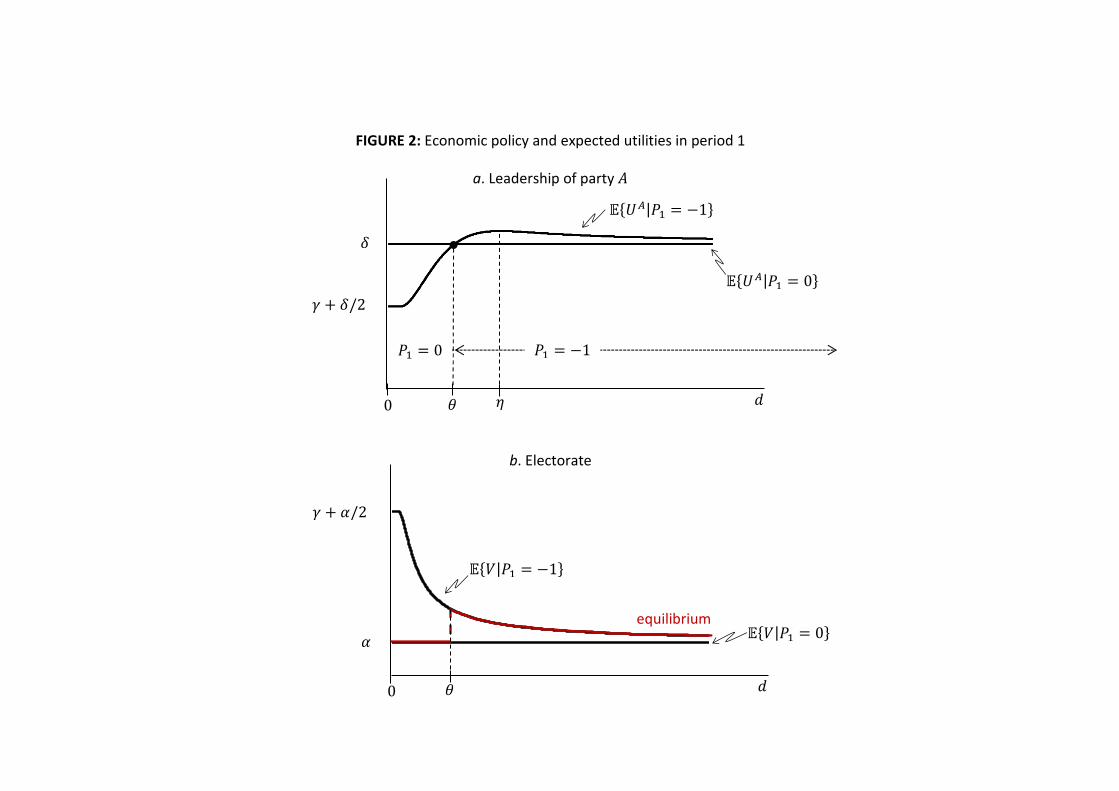
FIGURE 2: Economic policy and expected utilities in period 1

a. Leadership of party 𝐴

b. Electorate

equilibrium

𝜃

𝜂

𝔼{𝑉|𝑃1 = 0}

𝔼{𝑉|𝑃1 = −1}

𝛿

0 𝑑

𝛾 + 𝛿/2

0

𝔼{𝑈𝐴|𝑃1 = 0}

𝜃 𝑑

𝔼{𝑈𝐴|𝑃1 = −1}

𝑃1 = −1 𝑃1 = 0

𝛼

𝛾 + 𝛼/2

FIGURE 3: The election as a hypothesis test

a. Imprecise estimation (large 𝑑)

b. Precise estimation (small 𝑑)

chance of a type-I error = (1/2) ∙ gray-shaded area

chance of a type-II error = (1/2) ∙ red-shaded area

𝑢𝑣 − 1/𝑣

𝑢𝑣 − 1/𝑣 𝑢𝑣 + 1/𝑣

𝑢𝑣 + 1/𝑣 ε1𝑛/𝑑

휀1𝑛/𝑑