better machine learning models with multi-objective

Better Machine Learning Models with

Multi-Objective Optimization

Dr. Ingo Mierswa

RapidMiner | Real Data Science, Fast and Simple | 2

The Basics of Feature SelectionFeature selection can greatly improve your machine learning models. In this eBook, I outline all you need to know about feature selection. In Part 1 I discuss why feature selection is important, and why it’s in fact a very hard problem to solve. I detail some of the different approaches which are used to solve feature selection today.

Why Should We Care About Feature Selection?There is a consensus that feature engineering often has a bigger impact on the quality of a model than the model type or its parameters. Feature selection is a key part of feature engineering, not to mention Kernel functions and hidden layers are performing implicit feature space transformations. Therefore, is feature selection then still relevant in the age of support vector machines (SVMs) and Deep Learning? Yes, absolutely.

First, we can fool even the most complex model types. If we provide enough noise to overshadow the true patterns, it will be hard to find them. The model starts to use the noise patterns of the unnecessary features in those cases. And that means, that it does not perform well. It might even perform worse if it starts to overfit to those patterns and fail on new data points. This is made even easier for a model with many data dimensions. No model type is better than others in this regard. Decision trees can fall into this trap as well as multi-layer neural networks. Removing noisy features can help the model focus on relevant patterns.

But there are other advantages of feature selection. If we reduce the number of features, models are generally trained much faster. And often the resulting model is simpler and easier to understand. We should always try to make the work easier for we model. Focus on the features which carry the signal over those that are noise and we will have a more robust model.

Part 1


Why is this a Hard Problem?Let’s begin with an example. Let’s say we have a data set with 10 attributes (features, variables, columns) and one label (target, class). The label column is the one we want to predict. We’ve trained a model on this data and determined the accuracy of the model built on data is 62%. Can we identify a subset of those 10 attributes where a trained model would be more accurate?

We can depict any subset of 10 attributes as bit vectors, i.e. as a vector of 10 binary numbers 0 or 1. Zero means that the specific attribute is not used, and 1 depicts an attribute which is used for this subset. If we want to indicate that we use all 10 attributes, we would use the vector (1 1 1 1 1 1 1 1 1 1). Feature selection is the search for such a bit vector that produces the optimal accuracy. One possible approach for this would be to try out all the possible combinations. Let’s start with using only a single attribute. The first bit vector looks like this:

As we can see, when we use the first attribute we come up with an accuracy of 68%. That’s already better than our accuracy with all attributes, 62%. But can we improve this even more? Let’s try using only the second attribute:

Still better than using all 10 attributes, but not as good as only using the first.

We could continue to go through all possible subsets of size 1. But why we should stop there? We can also try out subsets of 2 attributes now:

Using the first two attributes immediately looks promising with 70% accuracy. We can collect all accuracies of these subsets until we have tried all of the possible combinations:

We call this a brute force approach.

How many combinations did we try for 10 attributes? We have two options for each attribute: we can decide to either use it or not. And we can make this decision for all 10 attributes which results in 2 x 2 x 2 x … = 210 or 1,024 different outcomes. One of those combinations does not make any sense though, namely the one which does not use any features at all. So, this means that we only need to try 210 – 1 = 1,023 subsets. Even for a small data set, we can see there are a lot of attribute subsets. It is also helpful to keep in mind that we need to perform a model validation for every single one of those combinations. If we use a 10-fold cross-validation, we need to train 10,230 models. It is still doable for fast model types on fast machines.


But what about more realistic data sets? If we have 100 instead of only 10 attributes in our data set, we already have 2100 – 1 combinations bringing the number combination to 1,267,650,600,228,229,401,496,703,205,375. Even the largest computers can no longer perform this.

Heuristics to the Rescue!Going through all possible attribute subsets is not a feasible approach then. We should however try to focus only the combinations which are more likely to lead to more accurate models. We could try to prune the search space and ignore feature sets which are not likely to produce good models. However, there is of course no guarantee that we will find the optimal solution any longer. If we ignore complete areas of our solution space, it might be that we also skip the optimal solution, but these heuristics are much faster than our brute force approach. And often we end up with a good, and sometimes even with the optimal solution in a much faster time. There are two widely used approaches for feature selection heuristics in machine learning. We call them forward selection and backward elimination.

Forward SelectionThe heuristic behind forward selection is very simple. We first try out all subsets with only one attribute and keep the best solution. But instead of trying all possible subsets with two features next, we only try specific 2-subsets. We try the 2-subsets which contain the best attribute from the previous round. If we do not improve, we stop and deliver the best result from before, i.e. the single attribute. But if we have improved the accuracy, we continue trying by keeping the best attributes so far and try to add one more. We continue this until we no longer have to improve.

What does this mean for the runtime for our example with 10 attributes from above? We start with the 10 subsets of only one attribute which is 10 model evaluations. We then keep the best performing attribute and try the 9 possible combinations with the other attributes. This is another 9 model evaluations then. We stop if there is no improvement or keep the best 2-subset if we get a better accuracy. We now try the 8 possible 3-subsets and so on. So, instead of going brute force through all 1,023 possible subsets, we only go through 10 + 9 + … + 1 = 55 subsets. And we often will stop much earlier as soon as there is no further improvement. We see below that this is often the case. This is an impressive reduction in runtime. And the difference becomes even more obvious for a case with 100 attributes. Here we will only try at most 5,050 combinations instead of the 1,267,650,600,228,229,401,496,703,205,375 possible ones.


Backward EliminationThings are similar with backward elimination, we just turn the direction around. We begin with the subset consisting of all attributes first. Then, we try to leave out one single attribute at a time. If we improve, we keep going. But we still leave out the attribute which led to the biggest improvement in accuracy. We then go through all possible combinations by leaving out one more attribute. This is in addition to the best ones we already left out. We continue doing this until we no longer improve. Again, for 10 attributes this means that we will have at most 1 + 10 + 9 + 8 + … + 2 = 55 combinations we need to evaluate.

Are we done? It looks like we found some heuristics which work much faster than the brute force approach. And in certain cases, these approaches will deliver a very good attribute subset. The problem is that in most cases, they unfortunately will not. For most data sets, the model accuracies form a so-called multi-modal fitness landscape. This means that besides one global optimum there are several local optima. Both methods will start somewhere on this fitness landscape and will move from there. In the image below, we have marked such a starting point with a red dot. From there, we continue to add (or remove) attributes if the fitness improves. They will always climb up the nearest hill in the multi-modal fitness landscape. And if this hill is a local optimum they will get stuck in there since there is no further climbing possible. Hence, those algorithms do not even bother with looking out for higher hills. They take whatever they can easily get. Which is exactly why we call those “greedy” algorithms. And when they stop improving, there is only a very small likelihood that they made it on top of the highest hill. It is much more likely that they missed the global optimum we are looking for. Which means that the delivered feature subset is often a sub-optimal result.

Slow vs. Bad. Anything Better Out There?This is not good then, is it? We have one technique which would deliver the optimal result, but is computationally not feasible. This is the brute force approach. But as we have seen, we cannot use it at all on realistic data sets. And we have two heuristics, forward selection and backward elimination, which deliver results much quicker. But unfortunately, they will run into the first local optimum they find. And that means that they most likely will not deliver the optimal result.

Don’t give up though – next we will discuss another heuristic which is still feasible even for larger data sets. And it often delivers much better results than forward selection and backward elimination. This heuristic is making use of evolutionary algorithms.


How do Evolutionary Algorithms work?Evolutionary algorithm is a generic optimization technique mimicking the ideas of natural evolution. There are three basic concepts in play. First, parents create offspring (crossover). Second, there is a chance that individuals undergo small changes (mutation). And third, the likelihood for survival is higher for fitter individuals (selection).

We now know that we can represent possible attribute subsets with bit vectors. We can represent the selection of all attributes of a data set which consists of 10 attributes in total such as (1 1 1 1 1 1 1 1 1 1). A bit vector for the subset which only uses the third attribute would be (0 0 1 0 0 0 0 0 0 0) instead.

The first step of an evolutionary algorithm is to create a population of individuals. This population will evolve over time. We call this the initialization phase of the evolutionary algorithm. The individuals in our starting population are randomly generated. And each individual is a bit vector like those described above. We create individuals by tossing a coin for each available attribute. Depending on the result we either include the attribute in this individual or not. There are no fixed rules for the size of a starting population. However, we should have at least 2 individuals in the population if we want to do crossover. A good rule of thumb is to use between 5% and 30% of the number of attributes as population size.

After we create the initial population, there is a series of steps we need to keep performing. That is until we reach a stopping criterion. The image to the right depicts one possible way to implement such a loop. Please note that there are different approaches for the implementation of evolutionary algorithms. Some people prefer to perform the selection only for crossover. Others first select a new generation and perform crossover afterwards. Some people mutate only the offspring, but others also mutate parents. In my experience, the exact details of the algorithm have only little effect on how well they perform so I will explain only one variant.

Step OneThe first step is to pick parents from our population for crossover. I prefer to randomly pick parents from my population until I use all parents in exactly one crossover. Since the selection of survivors happens directly before (see below), we do not need to use the fitness for the parent selection. The selection step will already make sure that we mate only fitter parents in the next generation. There are many variants to implement this.

There are also many variants for the actual crossover. The variant in the picture above uses a single split point at the same position for both parent bit vectors. We create the offspring by using the front part from the first parent combined with the back part of the second parent and vice versa. Crossover can lead to large jumps in the fitness landscape. These jumps allow evolutionary algorithms to cope much better with multi-modal fitness landscapes. They simply have less likelihood to get stuck in a local extremum.

Part 2


Step TwoThe next step is to perform mutation. Mutation means that we flip a single bit from 0 to 1 or the other way around. Many people only mutate the offspring of crossover, but I prefer to also mutate the parents. Please note that sometimes there is no mutation at all anyway. The likelihood for flipping the selection of a single attribute is 1 / m if m is the number of attributes. That means that we flip on average one attribute for each individual in the mutation. Mutation leads to a small movement in the fitness landscape. It can be useful to climb up towards a close-by extremum in the landscape. Finally, we can decide if we want to keep the original individuals as well or only keep the mutated individuals. I often keep both.

If we do decide to keep the original and the mutated individuals, then our population size is now 4 times bigger. We first created two new offspring from each pair of parents which doubled the population size. And then we created one mutation for each individual which doubles that population size again. In the next step, we should bring the population size down again to a smaller number. And we should prefer fitter individuals for survival while we are doing this.

Step ThreeBut first we will evaluate all individuals in our current population. We call this the evaluation phase of the evolutionary algorithm. We can, for example, use the accuracy of a cross-validated model trained on this feature subset. We store those accuracies together with the individuals, so we can perform a fitness-driven selection in the next step.

Step FourThe last step in our iterative process is selection. This step implements the concept of “survival of the fittest”. That means that individuals, i.e. attribute subsets, which lead to models with a higher accuracy should have a higher likelihood to survive. And survivors build the basis for new attribute sets in the next generation. There are many ways of performing a selection. We will in fact see in my next blog post that we have several interesting options for solving the feature selection problem in even better ways. But for now, we go with one of the most widely used selection schemes, namely tournament selection.

For tournament selection we pit a small group of individuals against each other. The fittest one of the group survives and makes it into the next generation. We use sampling with replacement for creating our tournament groups. This means that individuals can be also selected multiple times. We keep pitting individuals until the population of the next generation has reached the desired size again.

The group size has some impact on how likely it is that weaker individuals have a chance to survive. If the size of the tournament is equal to the population size, only the fittest individual will survive. But with a tournament size of only 2, even weaker individuals have a chance if they are up against another weak candidate. We can adapt the so-called selection pressure by picking different values for the tournament size. But be careful: too large and the algorithm might become too greedy. This increases the likelihood for sub-optimal results. But if the tournament size is too low, the optimization runs longer.

The loop ends when we meet a stopping criterion. This can be a maximum number of generations or the fact that there was no improvement any longer for some time. Or the optimization reached a time limit. But whatever the reason was, we deliver the best individual so far as result.


How Can We Easily Use Evolutionary Feature Selection?Let’s discuss how we can setup those different heuristics for feature selection in RapidMiner.

There have been numerous papers showing that evolutionary feature selection is effective. In this eBook, we want to show that the results of each of the different approaches can differ. We will use a single data set. Keep in mind that the approaches are heuristics and results can be completely different for other data sets, but in practice we will often see patterns like those we will discuss below.

The data set we will analyze is the Sonar data. It has 208 examples (rows, observations, cases…) and each one is a frequency spectrum of objects in the water. In total, we have 60 different frequency bands which form the attributes of our data set. Our goal is to detect from the frequency spectrum of an object if this object is a rock or a naval mine. The image below shows a visualization of the data in a parallel plot. Each line in this chart is representing one example in the data set. The color specifies if the corresponding object is a rock (blue) or a mine (red).

As we can see, this is a pretty hard task, but there are certain areas in the frequency spectrum where the two classes differ a bit more. These areas are even easier to see in the deviation chart below. This chart only shows the mean values for each attribute of both classes. The transparent regions represent the standard deviations of the attributes for each class.

There are 4 different areas of the frequency spectrum where the two classes differ most. Those are the areas around attribute 11, attribute 20, attribute 35, and attribute 45. We saw in the first image that a single area will be sufficient to find a good model. But some combination of attributes in those areas should help a lot to get over the noise.

https://1xltkxylmzx3z8gd647akcdvov-wpengine.netdna-ssl.com/wp-content/uploads/2017/11/post-3-process-1-multi-objective-feature-selection-on-sonar.zip


Process 1: Cross-Validation of Naïve Bayes on Complete Data (Benchmark)Before we do any feature selection, let’s first establish a benchmark by evaluating how well our model works on the complete data set. We will use Naïve Bayes as model type for the experiments here. And we will evaluate all models with the same 5-fold cross-validation. This means that there is no impact from different data splits during our experiments. We can do this in RapidMiner by defining a local random seed for the cross-validation operator.

We achieve 67.83% accuracy on the Sonar data set with Naïve Bayes. And of course, we expect that feature selection will improve the accuracy even further. We will not try the brute force approach here though. For the 60 attributes (frequency bands) of our data set, we would end up with 260 – 1 = 1,152,921,504,606,849,999 combinations.

Process 2: Forward SelectionThe next experiment we perform is a forward selection approach. We use the same 5-fold cross-validation as used above to evaluate the performance of each attribute subset. The optimization stopped already after 4 rounds and delivered attributes 12, 15, 17, and 18. The accuracy of this subset was 77.43%. This is much higher than our benchmark without any feature selection. But another thing is worth noticing. The feature selection has only selected attributes from the left two areas out of the 4 relevant areas of the frequency spectrum. The right two areas have not made it into the result. The forward selection simply stopped before after running into a local extremum.

Process 3: Backward EliminationWe will now try backward elimination as an alternative as it might do a better job in finding a good model considering all four important areas of the frequency spectrum. Unfortunately, this isn’t the case. This algorithm only removed 8 out of the 60 attributes from the data set. All other noise attributes stayed in the data set before the backward elimination was running into the first local extremum. The lower accuracy of only 73.12% should not come as a result then, although it is still better than using the full data. At least we can see that getting rid of those 8 attributes paid off already. But there is still too much noise in the data which covers the actual signals.

Follow Along!Make sure to have RapidMiner downloaded. Then download the processes here to build this machine learning model yourself in RapidMiner.

Process 1: Cross-validation of Naïve Bayes on Complete Data

Process 2: Forward Selection

Process 3: Backward Elimination

Process 4: Evolutionary Feature Selection

Please download the zip-file and extract its content. The result will be an .rmp file which can be loaded into RapidMiner via “File” 4 “Import Process”.

https://rapidminer.com/signup/

https://1xltkxylmzx3z8gd647akcdvov-wpengine.netdna-ssl.com/wp-content/uploads/2017/11/part-2.zip


Process 4: Evolutionary Feature SelectionLastly, let’s look at the evolutionary approach for feature selection. We use a population size of 20 and stop the optimization after a maximum of 30 generations. The optimization runs slightly longer than forward selection or backward elimination. But the accuracy is clearly higher: 82.72% and with that the best result we have achieved. What is equally interesting is the subset of 11 attributes selected by the algorithm:

attribute_6

attribute_11

attribute_12

attribute_16

attribute_20

attribute_21

attribute_28

attribute_36

attribute_39

attribute_47

attribute_49

This subset covers all four important areas of the frequency spectrum. We have attributes around attribute 11, attribute 20, attribute 35, and attribute 45. Which is exactly the reason why this feature selection has outperformed the other approaches. The evolutionary algorithm was simply not running into local extrema and stopped too early. It kept going until it found a much better result.

Key TakeawayForget about forward selection and backward elimination. Evolutionary feature selection should be the technique used to solve this problem. Next I discuss how we can get better results and additional insights by not only optimizing for the most accurate model alone. Instead, we will also optimize for the simplest model at the same time.


In Part 1 and Part 2, we discussed why feature selection is a great technique for improving your models. By having the model analyze the important signals, we can focus on the right set of attributes for optimization. As a side effect, less attributes also mean that you can train your models faster, making them less complex and easier to understand. Finally, less complex models tend to have a lower risk of overfitting. This means that they are more robust when it comes to creating the predictions for new data points.

We also discussed why a brute force approach to feature selection is not feasible for most data sets and tried multiple heuristics for overcoming the computation problem. We looked at evolutionary algorithms which turned out to be fast enough for most data sets. And they have a higher likelihood to find the optimal attribute subset.

So, we’ve found the solution then, right? Well, not quite yet.

Part 3Regularization for Feature SelectionSo far, we have been optimizing for model accuracy alone. We know from regular machine learning methods that this is a bad idea. If we only look for the most accurate model on the training data it will lead to overfitting. Our models will perform worse on new data points as a result. Most people only think about overfitting when it comes to the model itself. We should be equally concerned about overfitting when we make any decision in data analysis.

If we decide to merge two data sets, take a sample, or filter down the data, we are making a modeling decision. In fact, a more sophisticated machine learning model could have made this decision on its own. We need to be careful about overfitting and validating all decisions, not just the model itself. This is the reason it does not make sense to separate data preparation from modeling. We need to do both in an integrated fashion, and validate them together.

It doesn’t matter if we do feature selection automatically or manually. Any selection becomes a part of the model. And as such it needs to be validated and controlled for overfitting. Learn more about this in our blog series on correct validation.

We need to perform regularization to control overfitting for feature selection, just like we do for any other machine learning method. The idea behind regularization is to penalize complexity when you build models. The concept of regularization is truly at the core of statistical learning. The image below defines regularized risk based on the empirical risk and the structural risk. The empirical risk is the error we make on the training data. Which is simply the data we use for doing our feature selection. And the structural risk is a measurement of complexity. In case of an SVM the structural risk would be a low width of the margin. In case of feature selection it is simply the number of features. The more features, the higher the structural risk. We of course want to minimize both risks, error and complexity, at the same time.

https://rapidminer.com/blog/validate-models-training-test-error/


Minimizing the number of features and maximizing the prediction accuracy are conflicting goals. Less features means reduced model complexity. More features mean more accurate models. If we can’t minimize both risks at the same time, we need to define which one is more important. This is necessary so we can decide in cases where we need to sacrifice one for the other.

When we make decisions dealing with conflicting objectives, we can introduce a trade-off factor. This is the factor “C” in the formula above. The problem is that we cannot determine C without running multiple experiments. What are the possible accuracy ranges we can reach with our models on the given data set? Do we need 10 or 100 features for this? We can define C without knowing those answers. We could use hold-out data set for testing and then try to optimize for a good value of C, but that takes time.

Wouldn’t it be great if we didn’t have to deal with this additional parameter “C”? Finding a complete range of potential solutions. Some models would be great for lots of accuracy while others would use as little attributes as possible. And then of course some solutions for the trade-off in between. At this point, we also want to use an automated algorithm in a fast and feasible way.

The good news: this is exactly the key idea behind multi-objective optimization. We will see that we can adapt the evolutionary feature selection from our previous post. Once we do that, our model will deliver all good results rather than a single solution.

Or… You Just Optimize for Both SimultaneouslyWe want to maximize the accuracy and minimize the number of features at the same time. Let’s begin by drawing this solution space so that we can compare different solutions. The result will be an image like the one below. We use the number of features on the x-axis and the achieved accuracy on the y-axis. Each point in this space is now representing a model using a specific feature set. The orange point on the left, for example, represents a model which uses only one feature. And the accuracy of this model is 60% (or “0.6” like in the image).

Is the point on the left now better or worse than the other ones? We do not know. Sometimes we prefer less features which makes this a good solution. Sometimes we prefer more accurate models where more features work better. One thing is for sure, we want to find solutions towards the top left corner in this chart. Those are the models run with as little features as possible, and are also the most accurate. This means that we should prefer solutions in this corner over those more towards the bottom right.


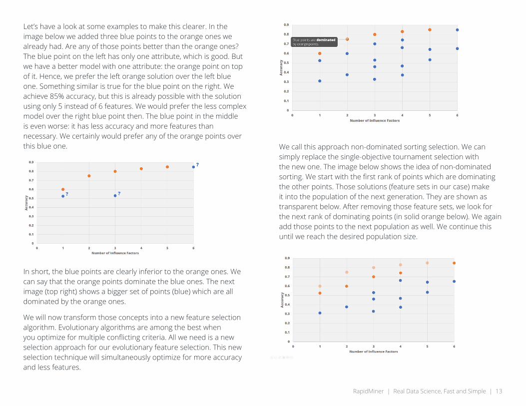
Let’s have a look at some examples to make this clearer. In the image below we added three blue points to the orange ones we already had. Are any of those points better than the orange ones? The blue point on the left has only one attribute, which is good. But we have a better model with one attribute: the orange point on top of it. Hence, we prefer the left orange solution over the left blue one. Something similar is true for the blue point on the right. We achieve 85% accuracy, but this is already possible with the solution using only 5 instead of 6 features. We would prefer the less complex model over the right blue point then. The blue point in the middle is even worse: it has less accuracy and more features than necessary. We certainly would prefer any of the orange points over this blue one.

In short, the blue points are clearly inferior to the orange ones. We can say that the orange points dominate the blue ones. The next image (top right) shows a bigger set of points (blue) which are all dominated by the orange ones.

We will now transform those concepts into a new feature selection algorithm. Evolutionary algorithms are among the best when you optimize for multiple conflicting criteria. All we need is a new selection approach for our evolutionary feature selection. This new selection technique will simultaneously optimize for more accuracy and less features.

We call this approach non-dominated sorting selection. We can simply replace the single-objective tournament selection with the new one. The image below shows the idea of non-dominated sorting. We start with the first rank of points which are dominating the other points. Those solutions (feature sets in our case) make it into the population of the next generation. They are shown as transparent below. After removing those feature sets, we look for the next rank of dominating points (in solid orange below). We again add those points to the next population as well. We continue this until we reach the desired population size.


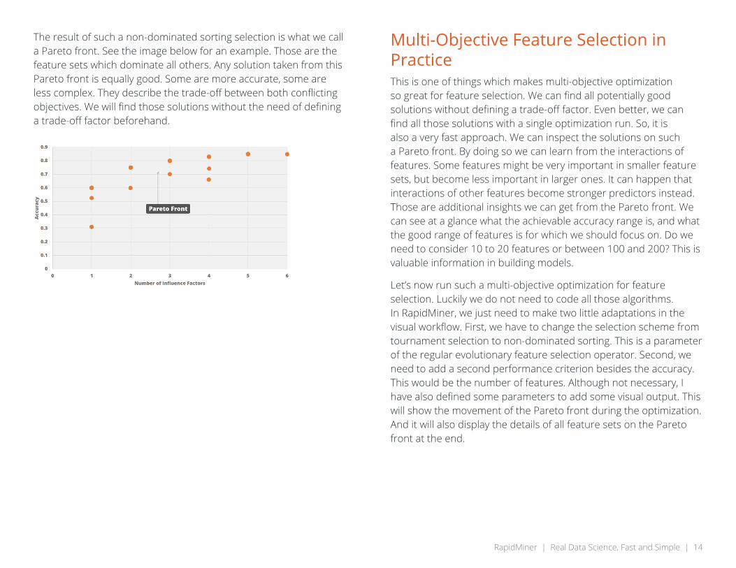
The result of such a non-dominated sorting selection is what we call a Pareto front. See the image below for an example. Those are the feature sets which dominate all others. Any solution taken from this Pareto front is equally good. Some are more accurate, some are less complex. They describe the trade-off between both conflicting objectives. We will find those solutions without the need of defining a trade-off factor beforehand.

Multi-Objective Feature Selection in PracticeThis is one of things which makes multi-objective optimization so great for feature selection. We can find all potentially good solutions without defining a trade-off factor. Even better, we can find all those solutions with a single optimization run. So, it is also a very fast approach. We can inspect the solutions on such a Pareto front. By doing so we can learn from the interactions of features. Some features might be very important in smaller feature sets, but become less important in larger ones. It can happen that interactions of other features become stronger predictors instead. Those are additional insights we can get from the Pareto front. We can see at a glance what the achievable accuracy range is, and what the good range of features is for which we should focus on. Do we need to consider 10 to 20 features or between 100 and 200? This is valuable information in building models.

Let’s now run such a multi-objective optimization for feature selection. Luckily we do not need to code all those algorithms. In RapidMiner, we just need to make two little adaptations in the visual workflow. First, we have to change the selection scheme from tournament selection to non-dominated sorting. This is a parameter of the regular evolutionary feature selection operator. Second, we need to add a second performance criterion besides the accuracy. This would be the number of features. Although not necessary, I have also defined some parameters to add some visual output. This will show the movement of the Pareto front during the optimization. And it will also display the details of all feature sets on the Pareto front at the end.


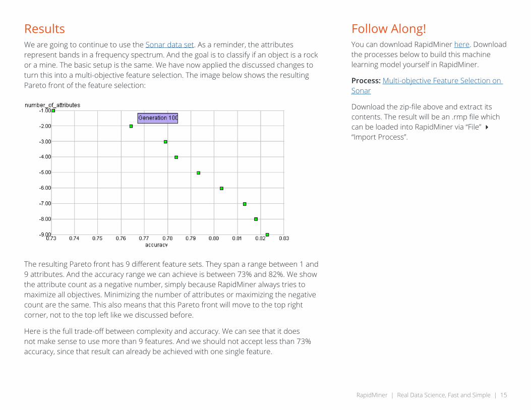
ResultsWe are going to continue to use the Sonar data set. As a reminder, the attributes represent bands in a frequency spectrum. And the goal is to classify if an object is a rock or a mine. The basic setup is the same. We have now applied the discussed changes to turn this into a multi-objective feature selection. The image below shows the resulting Pareto front of the feature selection:

The resulting Pareto front has 9 different feature sets. They span a range between 1 and 9 attributes. And the accuracy range we can achieve is between 73% and 82%. We show the attribute count as a negative number, simply because RapidMiner always tries to maximize all objectives. Minimizing the number of attributes or maximizing the negative count are the same. This also means that this Pareto front will move to the top right corner, not to the top left like we discussed before.

Here is the full trade-off between complexity and accuracy. We can see that it does not make sense to use more than 9 features. And we should not accept less than 73% accuracy, since that result can already be achieved with one single feature.

Follow Along!You can download RapidMiner here. Download the processes below to build this machine learning model yourself in RapidMiner.

Process: Multi-objective Feature Selection on Sonar

Download the zip-file above and extract its contents. The result will be an .rmp file which can be loaded into RapidMiner via “File” 4 “Import Process”.






It is also interesting to look further into the details of the resulting attribute sets. If we configure the workflow, we end up with a table showing the details of the solutions:

We again see the range of attributes (between 1 and 9) and accuracies (between 73% and 82%). We can gain some additional insights if we look into the actual attribute sets. If we only use one single feature, let it be attribute_12. But if we use two features, then attribute_12 is inferior to the combination of attribute_11 and attribute_36. This is another indicator why hill-climbing heuristics like forward selection have such a hard time.

The next attribute we should add is attribute_6. But we should drop it again for the attribute sets with 4 and 5 features in favor of other combinations. This attribute becomes interesting only for the larger sets again.

Finally, we can see that the largest attribute sets consisting of 8 or 9 attributes cover all relevant areas of the frequency spectrum. See the previous post for more details on this.

It is these insights which make multi-objective feature selection the go-to-method for this problem. Seeing good ranges for attribute set sizes or the interactions between features allow us to build better models. But there is more! We can use multi-objective feature selection for unsupervised learning methods like clustering.


Feature Selection for Unsupervised LearningIn part 1 of this eBook, we established that feature selection is a computationally hard problem. We then saw that evolutionary algorithms can tackle this problem in part 2. Finally, we discussed and that multi-objective optimization delivers additional insights into your data and machine learning model.

There’s one thing we haven’t discussed yet which is multi-objective feature selection. It can also be used for unsupervised learning. This means that you can now also identify the best feature spaces in which to find your clusters. Let’s discuss the problem in more detail and see how we can now solve it.

Part 4Unsupervised Feature Selection and the Density ProblemWe will focus on clustering problems for this part. Everything below is valid for most other unsupervised learning techniques as well.

Ok, let’s discuss k-means clustering for now. The idea of the algorithm is to identify centroids for a given number of clusters. Those centroids are the average of all features of the data points of their respective cluster. We then assign all data points to those centroids which – after some points have been re-assigned – will be recalculated. This procedure stops after either a maximal number of iterations or after the clusters stay stable and no point has been re-assigned.

So how can we measure how well the algorithm segmented our data? There is a common technique for this, namely the Davis-Bouldin index (or short: DB index). It can be calculated using the following formula:

with n as the number of clusters, ci as centroid of cluster i, σi as the average distance of all points of cluster i to their centroid, and d(ci,cj) as the distance between the centroids of clusters i and j.

As we can see, the result of a clustering is better if points within a cluster are close to each other. That of course is exactly what we wanted, but this also means that the DB index prefers clustering results where the clusters have a higher density.

But this preference for higher densities in the clusters is posing a problem for feature selection. If we do feature selection, we reduce the number of features. Less features also means higher densities in the remaining dimensions. This makes intuitive sense, because we map the data points from the higher-dimensional space into a smaller number of dimensions, bringing the points closer to each other.

Traditional feature selection cannot be used for clustering. Imagine that we have one feature as part of our data that is pure noise, but completely random. Say we flip a coin and use 0 for head and 1 for tails. We want to use k-means clustering with k=2 to find two clusters in our data and then decide to use forward selection to find the best feature set for this task. It first tries to find the best clusters using


only one feature. Of course, our random feature described above will win this race: it will produce two clusters with infinite density! One cluster will have all the points at 0 and the other one all the points at 1, but keep in mind that this was a complete random feature. As a result, clustering only using this dimension would be completely meaningless for the original problem and data space.

Even in cases where we don’t have a pseudo-categorical random feature, we will always pick only one feature. Namely the one which delivers the k densest clusters. Adding more features would only reduce the density again so we will not go there.

The Solution: Multi-Objective Feature SelectionCan multi-objective optimization help with this problem? Let’s do some experiments and see how this works. The data set below has four clusters in two dimensions: att1 and att2. There are also four additional random features called random1, random2 etc. The random features use a gaussian distribution of values around 0. Please note: the data is normalized so all data columns have mean 0 and standard deviation 1. This process is called standardization.

Here is how the data set looks if you only look at the dimensions att1 and att2:

It is easy to see the four natural clusters here. However, things change a bit if you plot the same data with the same point colors.

Follow Along!If you haven’t already, download RapidMiner here. Then you can download the processes below to build this machine learning model yourself in RapidMiner.

Please download the Zip-file and extract its content. The result will be a .rmp file which can be loaded into RapidMiner via “File” 4 “Import Process”.

Please note that you need to run the first three processes to create the data sets which will be used by the other processes. Please adapt the storage paths in the parameters of the storage and retrieval operators of all processes according to your setup.


https://1xltkxylmzx3z8gd647akcdvov-wpengine.netdna-ssl.com/wp-content/uploads/2018/01/process-files.zip


Below we use the dimensions random1 and random2 instead:

As expected, you can no longer see any clusters, and the data points are randomly scattered around the center. Before we even start with feature selection, let’s just run a k-means clustering with k=4 on the full data set consisting of all 6 features.

The clusters now represent the clusters found by k-means and they are not completely horrible. Still, the additional random attributes managed to throw off our k-means. On the left, you have the red and blue clusters completely mixed up and some of the red and blue points are even in the right clusters. Same is true for the yellow and green clusters on the right.

We can see that the noise attributes can render the clustering completely meaningless. The desired clusters have not been found. Since traditional feature selection is not helpful, let’s see how well a multi-objective approach will do.

We use the same basic setup like in the previous part. First, we retrieve the data set and then normalize the data as described above. We then use an evolutionary feature selection scheme where we use “non-dominated sorting” as the selection scheme.

The differences are a bit bigger inside of the feature selection operator:

Instead of using a 10-fold cross validation, we can create the clustering using k=4. The first performance operator takes the clustering result and calculates the DB-Index. The second operator calculates the number of features used for the current individual. We add this number as the second objective for our optimization.


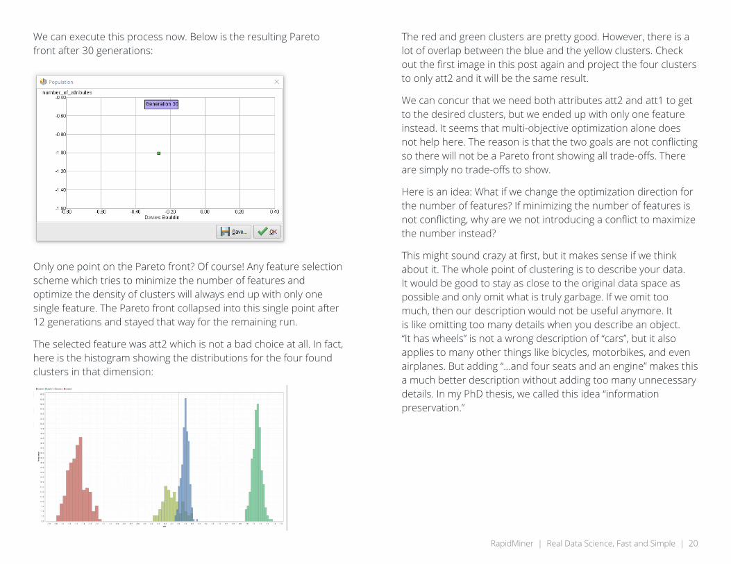
We can execute this process now. Below is the resulting Pareto front after 30 generations:

Only one point on the Pareto front? Of course! Any feature selection scheme which tries to minimize the number of features and optimize the density of clusters will always end up with only one single feature. The Pareto front collapsed into this single point after 12 generations and stayed that way for the remaining run.

The selected feature was att2 which is not a bad choice at all. In fact, here is the histogram showing the distributions for the four found clusters in that dimension:

The red and green clusters are pretty good. However, there is a lot of overlap between the blue and the yellow clusters. Check out the first image in this post again and project the four clusters to only att2 and it will be the same result.

We can concur that we need both attributes att2 and att1 to get to the desired clusters, but we ended up with only one feature instead. It seems that multi-objective optimization alone does not help here. The reason is that the two goals are not conflicting so there will not be a Pareto front showing all trade-offs. There are simply no trade-offs to show.

Here is an idea: What if we change the optimization direction for the number of features? If minimizing the number of features is not conflicting, why are we not introducing a conflict to maximize the number instead?

This might sound crazy at first, but it makes sense if we think about it. The whole point of clustering is to describe your data. It would be good to stay as close to the original data space as possible and only omit what is truly garbage. If we omit too much, then our description would not be useful anymore. It is like omitting too many details when you describe an object. “It has wheels” is not a wrong description of “cars”, but it also applies to many other things like bicycles, motorbikes, and even airplanes. But adding “…and four seats and an engine” makes this a much better description without adding too many unnecessary details. In my PhD thesis, we called this idea “information preservation.”


In fact, you only need to change one thing in the RapidMiner process above. The second performance operator has a parameter creatively called “optimization direction.” When we change this from “minimize” to “maximize” and we are ready to go. Below is the Pareto front we are getting at the end of this optimization run:

That looks much better, doesn’t it? We get five different points on this Pareto front. There is a clear difference for the DB index using only the first two attributes and the remaining solutions using 3, 5, or 6 features. What makes those first two solutions special then? Here is a table with the details about the solutions:

First, we get two times the same solution using only one attribute. We already know that att2 is the winner here having the best DB index. However, the next one is only slightly worse in terms of DB index and adds the “necessary” feature att1 as well. From there on, there is clear drop for the DB-Index when we start adding the random features.

There is no way to make the final choice of a cluster set without inspecting the resulting clusters. But now we can at least see if they make sense and describe our data in a meaningful way. It is often a good idea to start at those areas short before clear drops for the DB-index. This is not dissimilar to the known elbow criterion for selecting the best number k of clusters. We can clearly see the shape of this drop-off in the Pareto front chart above.

Thanks to the information-preserving nature of the approach, it delivers all relevant information. And you get this information in one single optimization run. Feature selection for unsupervised learning has been finally solved.


ConclusionEven in the age of deep learning, there are still a lot of applications where other model types are superior or preferred. Additionally, in almost all cases those models benefit from reducing the noise in the input data by dropping unnecessary features. Models are less prone to overfitting and become simpler which makes them more robust against small data changes. Also, the simplicity improves understandability of the models a lot.

Evolutionary algorithms are a powerful technique for feature selection. They are not getting stuck in the first local optimum such as forward selection or backward elimination. This leads to more accurate models.

An even better approach is using a multi-objective selection technique. These algorithms deliver the full Pareto front of solutions in the same runtime. We can inspect the trade-off between complexity and accuracy yourself (“is it really worth to add this additional feature?”) and you will get additional insights about the interaction of the features.

Finally, this multi-objective feature selection approach has another advantage. We can use it for unsupervised learning like for clustering techniques. However, we need to change the optimization direction for the number of features. This can be easily seen when maximizing density-based cluster measurements. If we simultaneously also minimize the number of features, we end up with only one single attribute, but if we maximize the number of attributes, it is harder to find dense clusters for more features. This will lead to the best clusters for all sensible numbers of features. We also preserve the original information which is what clustering is all about: find the hidden segments in your original data.

Here we have it: the one and only feature selection solution needed in the future.

Dr. Ingo MierswaFounder & President of RapidMiner

Ingo Mierswa is an industry-veteran data scientist since starting to develop RapidMiner at the Artificial Intelligence Division of the TU Dortmund University in Germany. Mierswa, the scientist, has authored numerous award-winning publications about predictive analytics and big data. Mierswa, the entrepreneur, is the founder of RapidMiner.


RapidMiner builds software for real data science, fast and simple. We make data science teams more productive through a lightening fast platform that unifies data prep, machine learning, and model deployment. More than 300,000 users in over 150 countries use RapidMiner products to drive revenue, reduce costs, and avoid risks.

For more information, visit www.rapidminer.com

10 Milk Street, 11th Floor Boston, MA 02108

©2018 RapidMiner, Inc. All rights reserved

better machine learning models with multi-objective

Documents