best practices in overset grid generation · best practices in overset grid generation william m....

BEST PRACTICES IN OVERSETGRID GENERATION

William M. ChanNASA Ames Research CenterMoffett Field, CA 94035

Reynaldo J. Gomez IIINASA Johnson Space CenterHouston, TX 77058

Stuart E. RogersNASA Ames Research CenterMoffett Field, CA 94035

Pieter G. BuningNASA Langley Research CenterHampton, VA 23681

AIAA 2002-3191

32nd AIAA Fluid Dynamics Conference24-26 June, 2002 / St. Louis, Missouri

For permission to copy or to republish, contact the copyright owner named on the first page.For AIAA-held copyright, write to AIAA Permissions Department,

1801 Alexander Bell Drive, Suite 500, Reston, VA 20191-4344.

AIAA 2002-3191

BEST PRACTICES IN OVERSET GRID GENERATION

William M. Chan �

NASA Ames Research Center

Mo�ett Field, California 94035

Reynaldo J. Gomez III y

NASA Johnson Space Center

Houston, Texas 77058

Stuart E. Rogers z

NASA Ames Research Center

Mo�ett Field, California 94035

Pieter G. Buning x

NASA Langley Research Center

Hampton, Virginia 23681

Abstract

Grid generation for overset grids on complex geom-etry can be divided into four main steps: geometryprocessing, surface-grid generation, volume-grid gen-eration and domain connectivity. For each of thesesteps, the procedures currently practiced by experi-enced users are described. Typical problems encoun-tered are also highlighted and discussed. Most of theguidelines are derived from experience on a varietyof problems including space access and return vehi-cles, subsonic transports with propulsion and high-liftdevices, supersonic vehicles, rotorcraft vehicles, andturbomachinery.

1. Introduction

One of the �rst applications of overset-gridtechniques1 to complex geometries took place in1988 on the Integrated Space Shuttle Launch Vehi-cle (SSLV). The �rst computations were performed ona highly simpli�ed model with less than a million gridpoints.2 Even for such a simple model, grid genera-tion consumed almost twelve man months. With notools available to build computational grids from CADmodels, special programs had to be written to con-struct some of the grids from CAD drawings. It was

�Computer Scientist, Senior Member, AIAAyAerospace Engineer, Member, AIAAzAerospace Engineer, Senior Member, AIAAxAerospace Engineer, Associate Fellow, AIAA

Copyright c 2002 by the American Institute of Aeronautics and Astro-

nautics, Inc. No copyright is asserted in the United States under Title 17, U.S.

Code. The U.S. Government has a royalty-free license to exercise all rights un-

der the copyright claimed herein for Governmental Purposes. All other rights

are reserved by the copyright owner.

clear that general purpose grid generation tools wereurgently needed to improve the process.

The second generation of SSLV grids3;4 were builton a CAD model with signi�cantly higher geometric�delity and contained about 16 million points. Ittook approximately two man years to create usinggeneral tools - ICEMCFD5 for geometry processingand surface-grid creation, HYPGEN6;7 for volume-gridgeneration and version 4 of PEGASUS8 for domainconnectivity. Concepts on the methods and toolsneeded to speed up grid generation were beginningto emerge, including the initial hyperbolic surface-gridgeneration development for complex geometries9 andcollar-grid applications.10 Geometry clean-up in theCAD package alone devoured one of the two totalman years. Surface grids were created using algebraicand elliptic methods on the CAD and required heavyuser's e�ort. The use of hyperbolic methods broughtsigni�cant savings in volume-grid generation time. Itwas recognized that such methods are best suited totake advantage of the exibility of the overset-grid ap-proach. The domain-connectivity input �le requiredthousands of lines of manual input and was anotherplace where improvements were desperately needed.

The Advanced Subsonic Technology Program playeda key role in driving the next phase in overset-analysisprocess development. The NASA IGES format11

was introduced and employed for some of the ge-ometry �les. CAD tools such as ICEMCFD andPro/ENGINEER were used for geometry processing.Hyperbolic surface grids were beginning to be usedfor some of the components. It was also important

1

American Institute of Aeronautics and Astronautics

to be able to duplicate the entire process quickly forslight design changes. This brought about the develop-ment of grid-generation scripts where important gridattributes were parameterized. Advances in variousparts of the process resulted in a grid-generation timeof 48 man days for a 22 million point grid system on acomplete subsonic-transport airplane with propulsionand high-lift devices.12 More than two-thirds of thegrid generation time was spent on domain connectiv-ity. Valuable experience was gained on the grid qualityrequired to attain accurate lift and drag predictions.

Key drivers in the further development of oversettools in the late 1990's came from the DOD HighPerformance Computing and Modernization Programand NASA's High Performance Computing and Com-munications Program. These programs supported thedevelopment of a comprehensive graphical user inter-face OVERGRID13 which serves as a uni�ed environ-ment for performing most of the grid-generation tasks.Major upgrades also occurred for two domain connec-tivity programs: version 5 of PEGASUS14 and DCFwith object X-rays.15 Applications involving complexgeometries were routinely performed starting from aCAD model. Highly complex grid systems such as theV-22 Tiltrotor, Comanche, subsonic-commercial air-planes could be produced in a few weeks.

Although the e�ort needed to perform overset-gridgeneration on complex geometries has been signi�-cantly reduced, state-of-the-art tools still require theuser to make key decisions and to enter some inputs.This paper describes the procedures practiced by ex-perienced users in overset-grid generation today. Sincethe software tools and algorithms are still evolvingtowards more automation and robustness, more andmore of the guidelines given in this paper are expectedto be automated in the future. In any case, a newoverset-grid user should be able to follow the stepsdescribed in this paper to generate high quality over-set grids. Advanced users may �nd this paper to bea useful collection of the current best practices. Theprinciples discussed here are independent of the soft-ware tools used, but examples will be given on toolsthat try to follow these principles.

The grid-generation process can be decomposed intofour main steps: geometry processing, surface-gridgeneration, volume-grid generation and domain con-nectivity. Details of each step are presented in Sec-tions 2 to 5. The overall strategy is to �rst createa clean surface-geometry de�nition on which overlap-ping surface grids can be generated. With suÆcientoverlap between surface grids, the volume grids canbe created easily with hyperbolic marching out to a�xed distance from the surface. The distance is cho-sen such that the outer boundaries of the near-bodyvolume grids are well clear of the boundary layer. Thenear-body volume grids are then embedded inside o�-body Cartesian grids that extend to the far �eld. Since

grid-generation strategies may di�er depending on theultimate goal of the simulation, issues related to thedi�erent goals will be discussed. Special attention willbe given to the treatment of airfoil shapes since theyoccur frequently in aerospace and marine applications.Best practices on the overall process are given in Sec-tion 6, and concluding remarks are given in Section 7.

2. Geometry Processing

Most grid-generation techniques require an under-lying geometry de�nition that represents the bound-aries of the objects about which computations are tobe performed. Input geometries can range from sim-ple analytic surfaces to computer-aided-design (CAD)generated solid models. These geometry de�nitionsare usually given to the computational uid dynam-ics (CFD) user in a variety of formats (Section 2.1).Unfortunately, most input geometries are usually in-appropriate in some way and require some work be-fore they can be used in surface-grid generation (Sec-tion 2.2). This step can be a very signi�cant bottleneckin the overall CFD process. Some experts estimatethat geometry repair can consume up to 80% of the to-tal time required for grid generation.16 Some examplesof geometry repair methods are given in Section 2.3.

2.1. Geometry Formats

Typical geometry database formats fall into two cat-egories (Fig. 1):

Analytic databasesThese usually contain CAD entities such as Non-

Uniform Rational B-Spline (NURBS) curves and sur-faces. Typical �le formats include Initial GraphicsExchange Speci�cation (IGES), Standard for the Ex-change of Product Model Data (STEP), and othernative CAD formats from individual vendors such asPro/ENGINEER.

Discrete databasesThese usually consist of a set of vertices with pre-

scribed connectivity to form a collection of quadrilat-erals or triangles. A bilinear representation of the sur-face based on these shapes is usually adopted. Com-mon examples include:

(1) Structured panel networks (multiple patcheswhere each patch contains a rectangular array ofquadrilaterals de�ned by a rectangular array ofvertices), e.g., PLOT3D17 format.

(2) Unstructured triangulated surfaces (unstruc-tured collection of triangles de�ned by anunstructured collection of vertices), e.g., Stere-olithography (STL), Drawing Exchange Format(DXF), Virtual Reality Markup Language(VRML), CART3D (http://www.nas.nasa.gov/~aftosmis/cart3d/cart3dTriangulations.html),FAST unstructured.18

2


(b)

(a)

(c)

Fig. 1 Analytic and discrete geometry databases.(a) CAD surfaces (analytic). (b) Multiple panelnetworks (discrete). (c) Surface triangulation (dis-crete).

Gridgen,19;20 OVERTURE21;22 and SURGRD9 allhave hyperbolic surface marching capabilities. SUR-GRD has the most mature hyperbolic marching capa-bility but is currently limited to marching on discretegeometry databases. Gridgen can march on CAD sur-faces and a future version will add the ability to useunstructured STL and VRML formats. A future ver-sion of OVERTURE will also introduce capabilities torepair and to march on CAD surfaces.23 Some commonoverset-grid-generation software and supported geom-etry formats are given in Table 1.

Ideally, surface grids should be generated on themost accurate representation of the geometry avail-able, which is typically a CAD geometry in IGES orSTEP format. The next best alternative is to use adiscrete database. These databases are typically pro-duced using standard manual grid generation tools orthrough in-house codes which can generate high qual-ity panel networks relatively automatically. Often themanual generation of a discrete-structured database,including any geometry repair, can be less time con-suming than the time required to repair a CAD �le.

Table 1.

Software Supported Geometry FormatsGridgen structured and unstructured

databases, IGES,native CAD import

ICEMCFD structured and unstructureddatabases, IGES,direct CAD interface

OVERTURE unstructured triangular formats,IGES

SURGRD/ structured and unstructuredOVERGRID databases: PLOT3D, CART3D,

FAST

2.2. Defects and Ideal Attributes

The input geometry should accurately represent theobjects being simulated. If the geometry representsan existing vehicle or wind-tunnel model, it should becompared with pictures of the as-built con�guration.Ideally a geometric veri�cation should be performedusing a 3D digitizer to insure that the computed ge-ometry matches the actual geometry. Missing gapsand protuberances can make the di�erence between apoor comparison and a good one. Minor geometric aws may cause local pressure variations but may nota�ect integrated forces and moments. Major aws,such as missing geometric features, can yield incorrectsolutions and can have serious consequences if they arenot detected.24

A model containing only relevant geometry shouldbe used as the input for grid generators. ProductionCAD models often include internal geometric compo-nents that do not come in contact with the ow �eld.Models can include wiring harnesses and fastener de-tails that will have a minimal in uence on the ow�eld but would require a large number of grid pointsto model. Ideally these details should be removed inthe original CAD system rather than in a CFD gridgenerator.A single valued, watertight geometry with consis-

tent normals can simplify grid generation. Many grid-generation techniques project points onto the underly-ing geometry database. Untrimmed, self-intersectingor overlapping surface geometry should be avoided

3


(c)

(a)

untrimmed surfaces

point to be projected

(b)

gaps

(d)

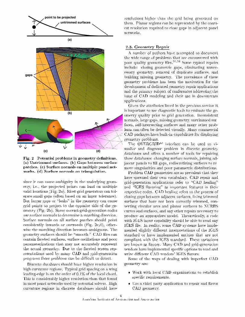
Fig. 2 Potential problems in geometry de�nitions.(a) Untrimmed surfaces. (b) Gaps between surfacepatches. (c) Surface normals on multiple panel net-works. (d) Surface normals on triangulation.

since it can cause ambiguity in the underlying geom-etry, i.e., the projected points can land on multiplevalid locations (Fig. 2a). Most grid generators can tol-erate small gaps (often based on an input tolerance).But larger gaps or \leaks" in the geometry can causegrid points to project to the opposite side of the ge-ometry (Fig. 2b). Some overset-grid-generation codesuse surface normals to determine a marching direction.Surface normals on all surface patches should pointconsistently inwards or outwards (Fig. 2c,d), other-wise the marching direction becomes ambiguous. Thegeometry surfaces should be \smooth." CAD �les cancontain faceted surfaces, surface oscillations and poorparameterizations that may not accurately representthe actual geometry. Due to the faceted screen rep-resentations used by many CAD and grid-generationprograms these problems can be diÆcult to detect.

Discrete databases should have higher resolution inhigh curvature regions. Typical grid spacing on a wingleading-edge is on the order of 0.1% of the local chord.This is considerably higher resolution than that foundin most panel networks used by potential solvers. Highcurvature regions in discrete databases should have

resolutions higher than the grid being generated onthem. Planar regions can be represented by the coars-est resolution required to close gaps in adjacent panelnetworks.

2.3. Geometry Repair

A number of authors have attempted to documentthe wide range of problems that are encountered withpoor quality geometry �les.25;26 Some typical repairsinclude: closing geometric gaps, eliminating unnec-essary geometry, removal of duplicate surfaces, andbuilding missing geometry. The prevalence of thesegeometry problems has been the motivation for thedevelopment of dedicated geometry repair applicationsand the primary subject of conferences addressing theissue of CAD modeling and their use in downstreamapplications.Given the attributes listed in the previous section it

is important to use diagnostic tools to evaluate the ge-ometry quality prior to grid generation. Inconsistentnormals, large gaps, missing geometry, untrimmed sur-faces, self-intersecting surfaces and many other prob-lems can often be detected visually. Many commercialCAD packages have built-in capabilities for displayinggeometry problems.The OVERGRID13 interface can be used to vi-

sualize and diagnose problem in discrete geometrydatabases and o�ers a number of tools for repairingthese databases: changing surface normals, joining ad-jacent panels to �ll gaps, rediscretizing surfaces to re-move singularities and poor parametric distributions.Problem CAD geometries are so prevalent that they

have spawned their own vocabulary. CAD repair andgrid-generation applications refer to \CAD healing"and \IGES avoring" as important features in theirrespective codes. CAD healing refers to the process ofclosing gaps between adjacent surfaces, �xing trimmedsurfaces that have not been correctly trimmed, con-verting circular arcs and planar surfaces to NURBScurves and surfaces, and any other repairs necessary toproduce an appropriate model. Theoretically, a codewith IGES input capability should be able to read anyIGES �le. In reality, some CAD systems have imple-mented slightly di�erent interpretations of the IGESstandard or have implemented entities that are notcompliant with the IGES standard. These variationsare known as avors. Many CAD and grid-generationvendors have implemented speci�c options to read andwrite di�erent CAD vendors' IGES avors.Some of the ways of dealing with imperfect CAD

geometry are:

� Work with local CAD organizations to establishspeci�c requirements.

� Use a third-party application to repair and avorCAD geometry.

4


� Use a grid-generation code that has a robust CADimport capability.

� Import native CAD format to avoid IGES issues.

� Interface directly to the native CAD system.

CAD�x from International TechneGroup Inc., Mil-ford, Ohio, and PlanetCAD's online service athttp://www.planetcad.com/index.html are two com-mercial options for geometry repair. CAD�x has aparticularly good range of geometry diagnostic and re-pair tools.

Gridgen has developed a robust capability to importand repair geometry by creating topology informationand \gluing" adjacent surfaces together based on inputnode and curve tolerances. The OVERTURE develop-ers have chosen to automate as much of the geometryrepair process as possible and are planning to providea set of geometry repair tools.22;23

Another solution to the CAD-import problem is toadd a direct CAD interface to the code. This al-lows the grid-generation software to work with a CADpart in its original format and potentially enablinggrid regeneration on parametrically varying surfaces.ICEMCFD, Inc. has developed versions of their grid-generation software that directly interfaces to a num-ber of commercial CAD systems.27 The CAPRI28 li-brary provides an application programmer's interfaceto several di�erent commercial CAD systems, simpli-fying the process of interfacing grid-generation codesto native CAD.

3. Surface-Grid Generation

Identify features

Decompose domain by features and gaps

Identify components

Decompose domain by components

Extract domain curve(s)

Create hyperbolic/algebraic surface grids

Distribute grid points on domain curve(s)

Trimmed Untrimmed

DoneNoYes Are there remaininggaps between grids

Fig. 3 Surface-grid generation procedure fortrimmed and untrimmed approach.

The goal of surface-grid generation is to create sur-face grids that capture both geometric and ow fea-tures with suÆcient resolution. A strategy for creatingoverset surface grids begins with this goal in mind and

can be carried out via the trimmed or untrimmed ap-proach (Fig. 3). In complex applications, surface gridsare usually generated using a mixture of the two ap-proaches. The trimmed approach follows the surfacefeatures, and places grid points only on the exposedsurfaces. The untrimmed approach follows the geo-metric components where some points may be placedon unexposed surfaces which will later be removed (seeSection 5).

One of the advantages of using overset grids is thatvarious components of a complex body can be added,removed or substituted without regridding the entirecon�guration. For example, in a fuselage/wing con-�guration, the untrimmed approach will identify thefuselage and the wing as separate components. Af-ter building a fuselage grid, a wing grid can be addedby punching a hole in the fuselage grid using a domainconnectivity program (Figs. 4a,b). This hole cutting isneeded because the fuselage is untrimmed in the vicin-ity of the wing. A collar grid is then used to �ll theresulting hole (Fig. 4c). Further analysis may requirethe introduction of a tail over the fuselage and a pylonand nacelle under the wing. A new design may requiresubstitution of the old wing with a new wing. In allsuch cases, existing grids do not have to be regener-ated, but holes will need to be created or modi�ed. Insome cases, if the components introduced are signi�-cantly smaller than the parent component, points onthe parent grid should be redistributed to match thatof the smaller component locally (see Section 3.4).

For the trimmed approach, the wing/fuselage in-tersection curve, the wing leading- and trailing-edgecurves, the symmetry-plane curve and the fuselagenose and tail apexes are identi�ed as surface features.In Fig. 4d, surface grids are built around these surfacefeatures. E�ectively, the fuselage is trimmed where thewing is to be attached. A wing grid can then be intro-duced without the need to cut a hole on the fuselage.As will be discussed in Section 5, domain connectivityis robust and highly automated on grid systems thatrequire no hole cutting other than that on the o�-bodyCartesian grids. The addition of new attachments dorequire a repartitioning of the parent grid with thetrimmed approach, which then results in more work.

In practice, it is diÆcult to anticipate all possiblecomponents that will be attached to a body. Careshould be taken at the start of an analysis to include asmany permanent attachments as possible to maximizeusage of the trimmed approach. Optional attachmentsare more conveniently added via the untrimmed ap-proach. For example, the vertical tail is an importantattachment to a space launch vehicle which shouldbe included with the trimmed approach. More de-tailed subsequent analysis may require the modelingof a small feedline between the fuselage and a booster.The feedline could be attached using the untrimmedapproach.

5


(a)

(b)

(c)

(d)

Fig. 4 Untrimmed versus trimmed approach forfuselage/wing con�gurations. (a) Untrimmed fuse-lage and wing. (b) Hole cut in fuselage due to wing.(c) Collar grid used to �ll fuselage/wing junction.(d) Fuselage grids for trimmed approach.

For both trimmed and untrimmed approaches, thesurface-grid generation procedure can be subdividedinto the following steps: feature/component identi�ca-tion, surface-domain decomposition, domain-curve(s)extraction, grid-point distribution and surface-gridcreation. These steps are presented in more detail inthe subsections below.

3.1. Feature/Component Identi�cation

For the trimmed approach, surface features of thegeometry are �rst identi�ed. These features are de-scribed by either curves or points.29 Examples of fea-ture curves include sharp edges on the surface, in-tersection curves between components, high curvaturecontours such as those along the leading edges of airfoilshapes, and open-boundary curves (Fig. 5). Examplesof feature points include the intersection of multiplefeature curves and an apex point such as that at theapex of a cone (Fig. 5). In order to accurately capturea feature curve, a grid line should be made to followthe curve. Similarly, a grid point should be placed ata feature point.The importance of a clean starting point in the ge-

ometry description is immediately felt in trying toidentify and extract surface features. Since these fea-tures frequently lie along the boundary between ad-

apex point

open boundary curve

sharp edge curve

high curvature contour

intersection curve

feature point

Fig. 5 Examples of surface-feature curves and fea-ture points.

jacent geometric patches, gaps between the patcheswould result in ambiguity in determining such features.For the untrimmed approach, components of the

geometry are �rst identi�ed. In most cases, the bound-aries of a component are clearly de�ned, e.g. wing,canard, nacelle, pylon, �n, feedline, etc. In some cases,it is not at all clear where one component ends andwhere another one begins, e.g., the outboard face ofthe tail �ns of the X-38 blends directly into the mainbody (Fig. 5).

3.2. Surface-Domain Decomposition

Surface-domain decomposition is the task of decom-posing the surface of a solid body into overlappingfour-sided domains suitable for surface-grid genera-tion. Three-sided domains are sometimes used nearsurface-feature points. An advantage of the overset ap-proach is that the boundaries of such domains can beplaced arbitrarily provided they allow suÆcient over-lap between neighboring grids (see Sections 3.4 and 5for more details on the overlap required). A domainwith complicated topologies tends to result in diÆcultsurface- and volume-grid generation and domain con-nectivity, and complex inputs for the ow solver. Also,a large number of small domains tends to reduce owsolver eÆciency. Therefore, the ideal surface decom-position should contain as few domains as possible toresolve the geometry, and that each domain should betopologically as simple as possible.

6


For the trimmed approach, relevant surface featuresshould be used as starting points for the design of asurface decomposition. For example, a feature curvecould form one of the boundaries of a four-sided do-main while the remaining boundaries are free oating.The exact locations of free- oating boundaries are usu-ally not known until the surface grid has been createdby hyperbolic marching from the �xed boundary. Fre-quently, a domain is built on each side of a featurecurve with the �nal surface grid built by combining thegrids from the two resulting domains. For example, acurve that lies along the wing/fuselage intersection inFig. 4 is used to construct a domain on the fuselageside and a domain on the wing side. Surface gridscreated in the two domains are combined to form asingle collar grid (Section 3.2.1). Work on automaticdomain decomposition near surface features has beenpresented in Ref. 29. However, the distances by whichsuch domains should extend from the surface featuresto maximize surface coverage are currently not auto-matically determined.

Frequently, domains built around the surface fea-tures do not �ll the entire surface geometry. Addi-tional domains need to be constructed in the gaps.Such gap domains are usually �lled by (1) creatingsurface curves that form the four boundaries of thedomain, and then the interior grid is generated bytrans�nite interpolation, or (2) creating one surfacecurve through the middle of the domain, and then sur-face grids on each side of the curve are generated byhyperbolic marching. An algorithm to automaticallyidentify and �ll such gaps is given in Ref. 30. Un-fortunately, this algorithm tends to generate a largenumber of small domains which can be ineÆcient for ow-solver processing.

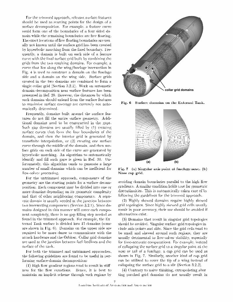
For the untrimmed approach, components of thegeometry are the starting points for a surface decom-position. Each component may be divided into one ormore domains depending on its geometric complexityand that of other neighboring components. A sepa-rate domain is usually needed at the junction betweentwo intersecting components (Section 3.2.1). Since do-mains designed in this manner will cover each compo-nent completely, there is no gap-�lling step needed asfound in the trimmed approach. For example, the Ex-ternal Tank surface is divided into 15 domains (someare shown in Fig. 6). Domains on the upper side arerequired to be more dense to communicate with theattach hardware and the Orbiter. Collar grid domainsare used at the junction between fuel feedlines and thesurface of the tank.

For both the trimmed and untrimmed approaches,the following guidelines are found to be useful in per-forming surface-domain decomposition:

(1) High ow-gradient regions tend to result in sti�-ness for the ow equations. Hence, it is best tomaintain an implicit scheme through such regions by

collar grid domains

Fig. 6 Surface domains on the External Tank.

(a) (b)

Fig. 7 (a) Singular axis point at fuselage nose. (b)Nose cap grid.

avoiding domain boundaries parallel to the high owgradients. A similar condition holds true for geometricdiscontinuities. This is automatically taken care of byfollowing the guidelines for the trimmed approach.

(2) Highly skewed domains require highly skewedgrid topologies. Since highly skewed grid cells usuallyresult in poor accuracy, their use should be avoided ifalternatives exist.

(3) Domains that result in singular grid topologiesshould be avoided. Singular surface-grid topologies in-clude axis points and slits. Since the grid cells tend tobe small and skewed around such regions, they areusually detrimental to ow-solver stability, especiallyfor time-accurate computations. For example, insteadof collapsing the surface grid to a singular point at thenose or tail of a fuselage, a cap grid can be used asshown in Fig. 7. Similarly, another kind of cap gridcan be utilized to cover the tip of a wing instead ofcollapsing the surface grid to a slit (Section 3.2.2).

(4) Contrary to naive thinking, extrapolating abut-ting patched grid domains do not usually result in

7


patch to be extended

Fig. 8 Patched grids that would result in pooroverset grids when extrapolated.

high quality overset domains. This is because patchedgrid domains frequently violate conditions (1) and (2)above. For example, a common practice of the patchedgrid approach is to place a domain boundary alonga geometric discontinuity. As shown in Fig. 8, ex-trapolating the indicated patch by hanging it over orwrapping it around the sharp edge on the left wouldresult in bad overset, i.e., the overset boundary runsparallel to and is close to a geometric discontinuity.From the patched grid viewpoint, it may seem likea burden to make grids overset. However, from theoverset viewpoint, the ability to freely place the gridboundaries (given the guidelines above) is a exibilitythat is most valuable.Surface-domain decomposition remains one of the

most diÆcult tasks to automate and relies heavily onthe experience of the user for an e�ective strategy. Theguidelines provided here should provide a start for fur-ther automation research.

3.2.1. Collar Grids

The concept of collar grids was originally intro-duced in the context of intersecting components usingthe untrimmed approach.10 The term is used todayto describe a grid around the junction between twocomponents for both the untrimmed and trimmed ap-proaches. With the trimmed approach, the collar gridis the result of combining the grids on each side ofthe intersection curve between two neighboring com-ponents. For the untrimmed approach, a collar grid isneeded to �ll the junction between two components. Inorder to understand why this is necessary, consider thewing/body example in Fig. 9. The untrimmed bodyvolume grid contains grid points that lie inside thewing and the untrimmed wing volume grid containsgrid points that lie inside the body. After removingthese non-physical grid points by hole cutting (Sec-tion 5), the junction between the components is left

(a) (b) (c)

Fig. 9 (a) Volume slice from untrimmed body.(b) Volume slices from wing and body after holecutting. (c) Volume slice and surface grid for collar.

(a) (b) (c)

Fig. 10 (a) Two collars in concave region. (b)Close-up view of left collar. (c) Close-up view ofright collar.

empty. The collar grid is introduced to �ll the gap inthis region.

Concave corners that arise from collar grid topolo-gies can pose a diÆcult problem for any volume-gridgenerator. In particular, generating a single volumegrid that completely �lls such a region can be toughor even impossible (Fig. 10). Opposite faces of thecorner will restrict the total distance that the grid canbe marched without overlapping itself. Breaking theconcave region into two or more overlapping grids cansigni�cantly simplify the volume gridding process andimprove the local grid quality by reducing the numberof constraints on the grid generator.

3.2.2. Airfoil Shapes

In aerospace and marine applications, airfoil shapesappear in many di�erent geometric components.These include wings, pylons, nacelles and tails in spacevehicles and airplanes, turbine blades in turbomachin-ery, slats and aps in high-lift devices, rotor blades

8


(a) (b)

(c) (d)

Fig. 11 (a) O-type tip cap (front view). (b) C-type tip cap (front view). (c) O-type tip cap (backview). (d) C-type tip cap (back view).

in rotorcraft, �ns and canards in missiles, and sailsin submarines. Choosing a grid topology is the �rstorder-of-business for any structured grid approach.For overset gridding of wings or other extruded shapes,there are two special regions, the root and the tip.As mentioned above, the wing root can be conve-

niently covered with a collar grid, with the streamwisetopology and grid spacing usually chosen to match themain-wing grid. In the spanwise direction, the gridwraps onto the fuselage as shown in Fig. 9c, conve-niently producing a collar grid with only one viscousdirection.The wing tip region is most e�ectively covered by a

tip cap grid. As opposed to closing the tip into a slitor trying to wrap the wing grid around the tip, thetip cap can resolve high gradients from the tip vor-tex while maintaining relatively smooth grid spacing.Again depending on the wing-grid topology, the capcan either wrap from the tip onto the wing trailingedge (O-type cap) or extend into the wake along thewake cut (C-type cap) (Fig. 11).With care, tip caps can also cover squared-o� tips

while preserving the sharp edge. This topology is use-ful for covering an engine pylon-shelf region (Fig. 12),or the ends of aps or control surfaces (Fig. 13). Tipcap grids can be generated using the \wingcap" toolin Chimera Grid Tools (CGT).31

One �nal issue on gridding wings is how to handleblunt (or �nite thickness) trailing edges. While ideal-ized wings have a sharp trailing edge, most real wingshave have a blunt trailing edge, requiring some grid ap-proach to handling this geometric feature. For caseswhere wake resolution is not critical, an O-grid can beused to wrap around the trailing edge. Otherwise, aC-grid topology can be utilized in one of several ways,

pylon shelf cap

nacelle

Fig. 12 Pylon-shelf cap grid.

Fig. 13 Flap end cap grid.

(a) (b)

Fig. 14 Finite thickness trailing edge grids. (a)Collapse in �rst wake point. (b) Wrap around thebase then to wake.

depending on the trailing-edge thickness compared tothe streamwise grid spacing at the trailing edge. Ifthe thickness is less than 0.2% of the local chord, itis recommended that the grid be continued aft of thetrailing edge and the gap closed in the �rst point inthe wake (Fig. 14a). If the trailing edge thickness isgreater than 0.2% chord, this approach can result intoo abrupt a change in grid spacing and direction. Analternative is to wrap the surface grid onto the baseand then out the wake (Fig. 14b).32;33 The drawbackto this second approach is that it tends to result inunsmooth, skewed grids.

3.3. Domain Curves Extraction

The surface grid for a domain may be created fromone or more bounding curves depending on how many

9


boundaries are �xed or are free to oat. Curves thatlie on �xed boundaries have to be extracted from thesurface geometry. Whether the trimmed or untrimmedapproach is taken, these are typically just the featurecurves of the geometry. For the trimmed approach,some domains are used to �ll the gaps between gridscreated from the surface features. All boundaries ofsuch domains are usually free oated. The numberof bounding curves to be extracted then depends onwhether a hyperbolic or algebraic method is employedfor grid generation (see Section 3.5 for further discus-sion).The domain curves extraction method is dependent

on the format of the geometry de�nition. For a CADgeometry description, curve extraction should be per-formed inside the same CAD tool from which the CADmodel is built. Sometimes feature curves, such asintersection curves, are already present in the CADde�nition. At other times, they have to be extractedmanually. If the geometry description is in the formof panel networks or triangles, surface features can beextracted using the algorithms and tools described inRef. 29. Automatic extraction is possible for sharpedges, intersection curves and open boundaries. Insuch cases, small manual clean up using a graphicalinterface is still necessary as extraneous curves are fre-quently produced as a result of poor surface resolutionon high curvature regions and gaps between surfacepatches. For high curvature contours, manual extrac-tion using a graphical interface such as OVERGRID isstill the most robust method.

3.4. Grid-Point Distribution

After extraction of the domain-bounding curve(s),grid points should be appropriately distributed onthese curves. The grid-point distribution should pro-vide suÆcient resolution of the surface geometry andsuÆcient overlap between neighboring domains (Sec-tion 5). A grid-induced truncation-error analysis34;35

could be used to diagnose grid-point-distribution qual-ity.Decisions on grid-point distribution usually begin

with the choice of a grid spacing for near-�eld reso-lution �sg . This is the typical grid spacing on thesmooth and at regions of the surface geometry andserves as the upper limit on the grid spacings of allsurface and volume grids in the near-body ow �eld.In other words, �ner grid spacings will be used in highsurface-curvature regions (e.g., leading edges), sharpconvex corners, and high ow-gradient regions. Thechoice of �sg directly a�ects the total number of gridpoints required in the con�guration and hence could bein uenced by the a�ordability of the simulation. Forexample, a one-inch near-�eld resolution may be de-sirable for a particular scenario, but limited time andcomputer resources may dictate a larger value.

(a)

(b)

Fig. 15 Surface and volume grid point distribu-tions at (a) convex, and (b) concave corners.

It is clear that grid clustering should be used wherethe geometry is changing rapidly in the convex sense,i.e., at convex high curvature regions and convex sharpcorners. The faster the change, the smaller the gridspacing needs to be to counteract the diverging e�ectof grid spacing in the volume grid around such a region(Fig. 15a). By the same token, grid spacings shouldnot be clustered into regions where the geometry ischanging in the concave sense since the volume gridlines tend to converge as they grow away from thesurface. Moreover, equal grid spacings and stretch-ing ratios should be used on both sides of a corner tomaintain a uniform resolution of the corner (Fig. 15b).

The truncation error induced by the grid is relatedto the grid stretching ratio.34 In order to minimizetruncation errors, a small stretching ratio should beused. Again, this is counter-balanced by the a�ord-ability of using a large number of grid points with asmall stretching ratio. In practice, a stretching ratioof 1.2 or below for surface grids and 1.3 or below forvolume grids is found to work well.

Section 2 already discussed the removal of irrele-

10


vant geometric features. Relevant geometric featuresshould therefore be represented adequately, no matterhow small. Most ow solvers utilize at least a 5 pointdi�erencing stencil (because even 3-point central dif-ferencing schemes also add a 5-point smoothing term)which implies that at least 5 points should be usedon any geometric feature. Obviously, similar sizedgeometric features at di�erent locations should be re-solved with similar grid-point distributions. Also, for ow solvers with multigrid options, a multigridablenumber of points (2n + 1) is preferred for each griddimension.One of the most important aspects of grid-point dis-

tribution is to ensure that the grid resolutions arecomparable in regions where inter-grid informationis exchanged. For overset grids, grid spacings fromneighboring grids in the overlapped zones should becomparable. A common mistake is to dump the wakeof an airfoil C-grid into a coarse background Cartesianmesh a short distance downstream from the airfoil.The coarse Cartesian mesh clearly cannot resolve the ow features passed on from the viscous spacing in theC-grid with the same �delity. Moreover, the C-gridalso receives poor resolution interpolation data fromthe coarse Cartesian mesh thus resulting in possibleupstream contamination (see Section 4.1.3 for furtherdiscussion). The grid spacing compatibility issue alsoarises when a small component is added to a largecomponent. For example, an analysis may �rst be per-formed on a wing with no pylon/nacelle attached. Thewing may have uniform spacing in the span direction.With the introduction of a pylon/nacelle attachment,the spanwise grid spacing around the pylon intersec-tion on the wing should be reduced to match the pylongrid spacing (Fig. 16). Higher spanwise resolution isalso needed to capture the high angle-of-attack owphysics caused by the nacelle.

3.4.1. Airfoil Shapes

Clustering for overset wing grids must satisfy geo-metric and ow-gradient requirements, as well as pro-vide adequate resolution in overlap regions for goodcommunication between grids. In that the major-ity of the wing surface can be covered with a singlegrid, many of these requirements are the same as forpatched/structured or unstructured grid approaches.Required clustering at wing leading and trailing

edges is determined by expected ow gradients. Forthe leading edge, this depends on the leading-edge ra-dius and the range of stagnation-point locations, buta rule of thumb is to use a grid spacing of 0.1% of thelocal chord.33 For the trailing edge, a spacing of 0.2%chord is recommended in order to capture the high owgradient associated with the equalization of upper andlower surface pressure. The use of 101 grid points onthe upper surface and 101 points on the lower surface

Fig. 16 Wing surface grid is re�ned near pylon at-tachment region to provide proper communicationwith pylon grids.

will avoid high grid stretching and maintain adequateresolution when using these leading- and trailing-edgeclusterings. More points may be needed for good com-munication between high lift elements or for precisecapturing of shocks, while fewer points can be used forlightly loaded components like pylons.In the spanwise direction, grid clustering for the

wing is determined by having suÆcient resolution tooverlap the wing-root collar and tip-cap grids. Typicalspacing in the root and tip overlap regions is 5% of thelocal chord. There may be additional requirements inthe middle of the wing due to geometry or expected ow gradients. For example, Fig. 16 shows a re�nedwing grid in the region of an underwing pylon/nacelle.

3.5. Surface-Grid Creation

The goal of surface-grid creation is to generate a sur-face grid from one or more supplied bounding curves ofthe domain. Grid points created during the griddingprocess should lie on the geometry de�nition, and gridcells should follow the guidelines of good mesh qualitysuch as orthogonality and stretching constraints. It isgood practice to do a quick check on surface-grid qual-ity prior to volume-grid generation, e.g., by looking ata graphical plot of grid quality functions as those foundin the OVERGRID interface.At the surface-domain decomposition step, the num-

ber of prescribed bounding curves for each domain isalready determined. By following the overset griddingstrategy described so far, domains with just one spec-i�ed bounding curve frequently arise, e.g., the collarand cap grids discussed in Section 3.2.2. Such casesare perfectly suited for hyperbolic surface-grid gener-ation methods.9 From the prescribed initial curve, the

11


surface grid is created by a marching scheme underorthogonality and cell area constraints. Side bound-aries are usually free oated or restricted to oat alonga given plane or curve. The boundary opposite theinitial curve is always free oated. Enforcing orthog-onality with the hyperbolic marching is not alwaysappropriate as in the case of growing a surface grid(part of a collar) onto a swept wing from the wingroot. The underlying geometry dictates that the gridlines be swept to follow isoparametric lines on thewing. In this situation, an algebraic marching schemeis preferred.9

Domains with two, three or four prescribed bound-ing curves could also arise in certain situations. Suchgrids are best treated with algebraic or elliptic meth-ods. Ref. 9 presents an implementation that usestrans�nite interpolation for the grid interior. Miss-ing bounding curves are �rst automatically created forcases with two or three prescribed boundaries. Theclass of grids associated with airfoil-shape componentsare good examples requiring such treatment. For in-stance, the leading- and trailing-edge curves of a wingare two opposite bounding curves for a surface grid onthe upper or lower surface of the wing. One could,of course, break the upper surface into two domains,each with only one prescribed bounding curve, and usehyperbolic marching from the leading-edge curve andthe trailing-edge curve respectively. However, in orderto preserve ow solver implicitness over such impor-tant shapes, it is preferable to model the airfoil shapein one domain in the streamwise direction.

4. Volume-Grid Generation

The goal of volume-grid generation is to �ll the ow�eld with discrete points �ne enough to resolve the uid ow around an object. Body-conforming vol-ume grids should clearly be used near the surface. Inthe normal direction, the grid spacing should be smallnear the body surface and should increase with dis-tance from the surface. For a simple object that canbe modeled with just one surface grid, it is appropri-ate to grow a single volume grid from the surface tothe far �eld. For more complex objects with multiplesurface grids, the near-body volume grids usually can-not uniformly �ll the three-dimensional space in thevicinity of the body due to grid-spacing stretching. Inorder to provide a uniform resolution of the near-body ow �eld, and to �ll any gaps that might exist betweenthe near-body volume grids, it is advantageous to growthese grids to just a short distance from the body, andthen embed the near-body grids in stretched Cartesiangrids that extend to the far �eld.The question then remains as to how far the near-

body volume grids should extend from the surface.Two criteria are typically used to determine an es-timate, with the second criterion applying only for

viscous ows. The �rst criterion is based on optimalinter-grid communication with the o�-body Cartesiangrids. With grid-spacing stretching in the normal di-rection, the normal grid spacing will increase withdistance from the surface until it reaches a value closeto the near-�eld resolution spacing �sg discussed inSection 3.4. Let Dm be the distance from the surfaceat which this occurs. At this distance, the volume cellsize is approximately �sg in all three directions since�sg is a typical cell size in the tangential directioninherited from the surface grids. Enclosing the near-body grids grown to a distance Dm inside a uniformo�-body Cartesian grid with spacing �sg would thenprovide optimal inter-grid communication, thus easingthe task of domain connectivity. Moreover, the Carte-sian grid could uniformly �ll any gaps that may occurbetween the near-body grids as the inter-grid overlapstarts to deteriorate with distance away from the sur-face under certain situations.

For viscous ows, it is advantageous to completelycapture any wall-bounded viscous e�ects (boundarylayers, etc.) by the �ne near-body grids. Supposethis requires that the near-body grids be grown to aminimum distance of Dv. If Dv is less than Dm, thenear-body grids should be allowed to grow to distanceDm to satisfy both criteria. If Dv is greater thanDm, grid stretching in the normal direction shouldbe halted at distance Dm, and extra uniformly-spacedgrid points (with �sg spacing) should be padded untildistance Dv is reached.

The far-�eld boundary of the o�-body Cartesiangrids should be positioned such that interference withthe near-�eld ow is minimized. The appropriate dis-tance from the body surface to the far-�eld boundarytypically depends on the speed of the free-stream ow,and on the importance of capturing body forces ac-curately. At low Mach numbers, this distance cangreatly a�ect the computed forces for a high-lift airfoilat maximum-lift conditions. Computational studiesin two dimensions showed a dependency of the liftand drag forces on the far-�eld distance up to about60 chord lengths.36 This dependency can be reducedthrough the use of a far-�eld boundary condition whichsimulates a point-vortex that matches the circulationof the airfoil ow. With this boundary condition, afar-�eld distance of 40 chord lengths was adequate. Inthree dimensions (3-D), the sensitivity to far-�eld dis-tance is less severe. For 3-D transonic ows, a typicalfar-�eld distance of about 20 body lengths is used. Forsupersonic ows, the far-�eld boundary can be placedmuch closer, e.g., about 10% of body length upstreamand one body length downstream. In this ow regime,accurate capturing of the bow shock by the volumegrids becomes an important issue.

12


4.1. Near-Body Grid Generation

The near-body volume grids should conform to thebody to provide proper modeling of the body ge-ometry. Tight normal-direction clustering should bemaintained near the wall to provide good boundarylayer resolution for viscous cases. Mesh orthogonal-ity should be maximized and grid stretching shouldbe minimized for better solution accuracy. All ofthe above desirable attributes could be accomplishedby using hyperbolic methods.6 Moreover, hyperbolicvolume-grid generation only requires the speci�cationof a surface grid while the remaining boundaries donot have to be prescribed. The hyperbolic-marchingscheme is computationally much cheaper than ellip-tic methods. Together, the simple inputs and eÆcientmarching scheme result in extremely fast grid genera-tion time.

With the surface grids already designed to pro-vide suÆcient overlap, this property is inherited bythe near-body volume grids in the vicinity of thebody. The overlap can be maintained away from thebody by applying a splay boundary condition on the oating boundaries of the volume grid during hyper-bolic marching. Several visualization tools, such asVisual337 and Fieldview,38 have the ability to createand display cutting planes through a collection of vol-ume grids for checking grid-overlap quality. This canbe a useful diagnostic tool prior to running a domain-connectivity code.

Typically the same wall spacing, marching distanceand total number of points are used for all near-bodygrids in the marching (normal) direction. Moreover,if the surface grids are designed with relatively simpletopologies, side boundary control (periodic, axis, con-stant plane, free oating) can be automated and thesame smoothing parameters could be employed for allgrids. For such cases, a multi-million point volume-grid system can be created in just a few minutes on atypical workstation or PC with almost no user inter-vention (Fig. 17).

It is important to ensure the volume grids have nonegative Jacobians and that the grids are of high qual-ity prior to proceeding to domain connectivity andthe ow solver. Since Jacobian computation is non-unique, the most appropriate check is to use the samealgorithm as that in the ow solver. For example, theHYPGEN7 tool contains a Jacobian calculator thatis identical to that used by the OVERFLOW39 owsolver. A quick visual inspection is also highly rec-ommended since having positive Jacobians for all cellsdoes not guarantee a properly formed grid, as shownin the self-intersecting case in Fig. 18.

Some considerations that arise for near-body volumegrids are discussed in the subsections below.

(a)

(b)

Fig. 17 Near-body volume grids and o�-bodyCartesian grid for X-38 V-131R vehicle. (a) Farview. (b) Close-up view showing marching distanceof near-body grids and grid spacing matching witho�-body Cartesian grids.

4.1.1. Viscous Wall Spacing

The requirements for the normal-direction spacingat the wall for viscous calculations depend heavily onthe Reynolds number and on the type of turbulencemodeling used. Although the boundary layer thicknesswill vary signi�cantly over the surface of a body, it is atypical practice to maintain the same wall spacing foran entire con�guration. Here the discussion is limitedto considerations of Reynolds-averaged Navier-Stokessolvers. Two-equation turbulence models often rec-ommend a wall spacing with y+ values less than one,where y+ is the non-dimensional turbulent distance.One equation turbulence models require a wall spac-

13


Fig. 18 Self-intersecting volume grid where all cellvolumes are positive.

ing given by y+ approximately equal to one. If wallfunctions are used, a signi�cantly larger wall spacingcan be used, corresponding to y+ between 35 and 100.The turbulent y+ distance can be estimated by us-

ing at plate formulas for either subsonic/transonic ows40 or supersonic/hypersonic ows.41 These formu-las are summarized as follows. Let

y+ =�wu

�y

�w(1)

where �w is the density at the wall, y is the physi-cal distance normal to the wall, �w is the viscosityat the wall, and u� is the friction velocity given byu� =

p�w=� where �w is the wall shear stress. As-

suming �w = �1 and �w = �1, we can write

y+ = Re

rcf2y (2a)

y =y+

Req

cf2

(2b)

where cf is the skin friction coeÆcient. It can be esti-mated from at-plate correlation40 as:

cf �0:455

ln2(0:06Rex)(3)

where Rex is the Reynolds number based on somedownstream distance x at which we wish to computey+. A typical choice would be at 10% of the referencelength, or x = 0:1 and Rex = 0:1�Re.This method gives reasonable values for subsonic

ow, and conservative values for higher Mach numbers.A more sophisticated model from Ref. 41 incorporatescompressibility as a function of free-stream temper-ature and Mach number. De�ning a compressibilityfactor fcomp and a reference temperature T �,

fcomp = 1 + 0:1157M21

(4a)

T �

T1= fcomp (4b)

A viscosity ratio is computed using Sutherland's law,and a compressibility correction rcomp is de�ned forthe Reynolds number:

��

�1=

�T �

T1

� 32

1 + S

T1T�

T1+ S

T1

!(5a)

rcomp =1

��

�1fcomp

(5b)

where the Sutherland constant S = 199ÆR for air. Thecompressible skin friction coeÆcient is then estimatedas

cf �0:455

ln2(0:06Rexrcomp)fcomp

(6)

The di�erence between free stream and wall condi-tions are accounted for as

TwT1

= 1 + � 1

2Pr

13M2

1(7a)

�w�1

=

�TwT1

� 32

1 + S

T1TwT1

+ ST1

!(7b)

�w�1

=

�TwT1

��1

(7c)

Typically the Prandtl number for air is taken as Pr =0:72.A modi�ed expression for the distance to the wall

can now be written as

y =y+

Req

cf2

0@ �w

�1q�w�1

1A (8)

Note that for M1 = 0 this equation reduces to thesimpler version in Eq. 2a, regardless of temperature.Typically, 20 to 30 points in the boundary layer is

considered good resolution. Besides viscous grid spac-ing, initial stretching also a�ects the accuracy of cal-culated skin friction. If the ow solver uses �rst-orderone-sided di�erencing for grid metrics at the wall, sev-eral points of constant spacing should be used.42 Forexample, Fig. 19 compares skin friction on a at platefor grids with 0, 2, and 5 cells of constant spacing atthe wall before beginning grid stretching. It can beseen that even 2 cells of constant spacing removes thestretching dependence on the skin friction.

4.1.2. One Versus Two Viscous Directions

In Section 3.2.2 a collar grid topology with onlyone viscous direction was discussed. This is adequatefor resolving integrated aerodynamic forces and mostcorner ow features. It simpli�es the use of a thin-layer viscous approach and avoids extremely small gridcells that result from grids which require viscous spac-ing in two directions (Such small cells can limit the

14


5 6 7 810 10 10 10

Re_x

-3

-2

10

10

Cf

0 cells const spacing2 cells const spacing5 cells const spacing

Fig. 19 Skin friction coeÆcient vs. plate Reynoldsnumber, for grids with 0, 2, and 5 cells of constantspacing next to the plate (solid line, dashed line,and �lled circles, respectively).

(a) (b)

Fig. 20 Slice of collar grid at fuselage/pylon junc-tion. (a) C-type topology (one viscous direction).(b) CH-type topology (two viscous directions).

stable time step, slowing convergence). One draw-back of the single viscous-direction approach is thetreatment for a wake cut of a C-grid collar. For thefuselage/pylon/nacelle topology shown in Fig. 20a, thefuselage in the wake of the pylon is represented as asolid surface plus a ow-through wake cut. Becauseof coordinate-direction di�erencing, the ow near thesurface may e�ectively see a partial grid-cell \tab" atthe root of the wake cut. At signi�cant angles-of-attack this can interrupt the smooth cross ow aroundthe fuselage, degrading the accuracy of the calcula-tion. This can be avoided by using an H-grid topologyin the spanwise direction (Fig. 20b), but results in acollar grid with two viscous directions.

4.1.3. C and O Grids and Wake Smoothing

While the choice of a C- or O-type grid for a winghas been referred to obliquely as a�ecting other gridchoices such as caps and collars, it is primarily a choicedetermined by the wing. Typically a C-grid is chosenfor wings to provide grid resolution in the wake regionand to avoid wrapping a grid around the obtuse an-gle of a sharp trailing edge. Conversely, con�gurations

0.01 0.02 0.03 0.04 0.05

CD

0.0

0.5

1.0

1.5

CL

Grid TypeO-GridC-Grid

Fig. 21 Drag polars for a NACA 0015 airfoil usingan O-grid (solid) and C-grid (dashed).

(a) (b)

(c) (d)

Fig. 22 Airfoil wake region. (a) Before smoothing(far view). (b) After smoothing (far view). (c)Before smoothing (close-up). (d) After smoothing(close-up).

where the wing wake does not impinge on other aero-dynamic surfaces, or for geometries with thick trailingedges such as space access or reentry vehicles, the wingmay be more conveniently resolved with an O-grid.Even for a relatively sharp NACA 0015 airfoil, Fig. 21shows a di�erence of only about 5% between O-gridand C-grid drag polars.

Another issue with C-grid wakes is viscous clusteringat the wake cut. It has been found that maintaining ay+ = 1 spacing in the wake can result in convergencediÆculties for some ow solvers (e.g., OVERFLOW).This cell spacing is unnecessarily small in the wake re-gion, and generally does not coincide with the actualwake. Furthermore, one typically stretches the stream-wise spacing aft of the trailing edge, resulting in gridcells with extremely large aspect ratios. One way to re-solve these problems is to smooth the grid in the wakeregion, relaxing the viscous clustering (Fig. 22). The\smogrd" tool in CGT31 can perform this function forwing, collar and wing cap grids.

15


Pylon InboardSlat

Krueger

Fig. 23 Leading edge devices in high-lift con�gu-ration.

4.1.4. Multi-Element Systems

High-lift aerodynamic analysis presents one of themost diÆcult challenges for CFD due to the com-plex geometry and complex ow physics. This stemsfrom the multiple bodies that make up the high-liftcomponents (wing, aps, slats, and various attach-ing hardware) and their large range of length scales.The small gaps between successive elements lead toboundary-layer and wake interactions, a complicatedviscous uid-dynamic phenomenon which greatly af-fects the performance of the high-lift system. Thiscomplex geometry and ow put speci�c constraints onthe volume-grid generation. The body-normal spac-ing must be �ne enough to resolve the wakes owingfrom upstream elements. Also, the spanwise spacingon the wing and aps must be �ne enough to resolvethe vortical structures formed at the spanwise ends ofthe leading-edge devices. Fig. 23 shows the leadingedge of a Boeing 777-200 aircraft43 in a high-lift con-�guration, near the engine pylon. The inboard slatand the Krueger slat can be seen, and the small gaps(both spanwise and streamwise) between the elementsare apparent.An example of the e�ect of the body-normal spacing

in resolving a high-lift ow �eld was shown previouslyby Rogers for ow computations about a three-elementairfoil.44 Fig. 24a shows a grid system with inadequatenormal spacing in the mesh around the downstreamelement. The hole in the downstream-element gridcaused by the upstream element is in an area wherethe normal spacing is too coarse. The grid pointsdenoted with circles are the only fringe points whichwill receive data interpolated from the wake of the up-stream element. They surround the wake, but thereare no points within the wake. This causes the down-stream grid to entirely miss the wake velocity defect,and hence compute too much mass ow in this region.This mass- ow error is passed back into the upstream-element grid when it receives interpolated data at itsdownstream outer boundary. This causes too muchmass to ow over the upper surface of the upstreamelement resulting in large errors in the computed pres-

(a)

(b)

Fig. 24 Close-up view of wake of upstream el-ement and upper surface of downstream element.(a) Grids with resolution mismatch. (b) Grids withmore resolution compatibility.

sure. An improved grid system for this geometry isshown in Fig. 24b, which has signi�cantly better gridresolution in the normal direction. It can be seen thatthere are more fringe points to resolve the wake ofthe upstream element. Results from this grid werereported by Rogers44 to be in good agreement withexperimental data.

4.2. O�-Body Cartesian Grid Generation

As already mentioned, it is advantageous to employuniform o�-body Cartesian grids to provide uniformresolution of important near-�eld ow features. Be-yond the near-�eld, stretched grids are used to extendthe computational domain to the far �eld. Two ap-proaches in use today are described below.The �rst approach encloses the near-body curvilin-

ear volume grids with a small number of Cartesiangrids. Each of these Cartesian grids has a uniformcore region that completely encloses some componentsof the near-body grids, and contains stretched outerlayers that extend away from the body (Fig. 17). Thefar �eld can be resolved with either a large coarseCartesian grid or with a curvilinear grid with ellip-soidal topology (Fig. 25).The second approach utilizes many Cartesian grids

16


Fig. 25 O�-body Cartesian grid and ellipsoidal far�eld grid.

Fig. 26 O�-body Cartesian grids with successivelevels of re�nement by proximity to body.

with successive levels of re�nement.45 These grids are�rst generated automatically based on proximity tothe body where the grid spacing of the �rst and �nestlevel is matched to the near-�eld grid resolution �sg .The grid spacings are coarsened by a factor of two foreach level of the outer layers which extends to the far�eld (Fig. 26). All levels of these Cartesian grids canbe modi�ed to adapt to the solution.

Both approaches are highly automated and providevery good results if the main purpose of the simula-tion is the accurate prediction of forces and moments.If o�-body ow features such as shocks need to becaptured accurately, the second approach is clearlymore appropriate. However, it also tends to be more

expensive due to a higher volume of inter-grid commu-nication between a larger number of grids.

5. Domain Connectivity

The task of domain connectivity consists of threeprocesses: projection, hole cutting, and fringe-pointinterpolation. Projection involves shifting surfacepoints to remove the e�ect of surface-discretization er-rors. Hole cutting is the removal of grid points fromone grid that reside inside the solid wall of anothergrid. The exibility of allowing neighboring grids toarbitrarily overlap often results in these situations.Fringe points are boundary points which are to be up-dated by the ow solver using interpolated solutiondata from a neighboring grid. Fringe points arise fromtwo sources: at the outer boundary of each grid whereno ow-solver boundary conditions are speci�ed, andat the boundary of holes. A valid interpolation sten-cil needs to be provided for each fringe point. If avalid interpolation cell cannot be obtained for a fringepoint, this is called an orphan point. Orphan pointscan occur where the hole-cutting operation removestoo many points, too few points, or where there is in-adequate overlap between neighboring overset grids.There are a number of di�erent software pro-

grams which were written to perform these oversetdomain-connectivity tasks. A partial list of thesecodes includes: PEGSUS4,8 PEGASUS5,14 DCF,15

BEGGAR,46�49 CHALMESH,50 OGEN,51 and soft-ware from the CFDRC corporation.52

5.1 Projection

Surface to surface projection is an issue for oversetgrids because of discretization errors. When two dif-ferent overlapped meshes discretize the same curvedanalytic surface, they each represent a di�erent ap-proximation to the original surface. Thus at any pointin the ow volume above the solid body, each meshwill have a di�erent measure of the distance from thispoint to its own discrete surface. Consider the sim-pli�ed representation of a two-dimensional mesh ona curved surface shown in Figs. 27a and 27b, wherethe body-circumferential direction has been immenselycompressed in scale in relation to the body-normaldirection. This way the �gure can represent the high-aspect ratio grid cells typically found in high Reynolds-number simulations, where the tangential spacing istypically on the order of 100 to 1000 times the normalspacing at the wall. The circular arcs in the �guresrepresent the exact surfaces; the 3x7 meshes repre-sents a subset of a donor mesh; and the circles drawnalong a wall-normal line represent fringe points froma neighboring mesh.In Fig. 27a, it can be seen that the �rst fringe point

above the surface actually lies in the �fth donor cell

17


(a) (b)

Fig. 27 Discrete surface mismatch on a curvedsurface. (a) Convex surface. (b) Concave surface.

above the surface. In actual high-Reynolds numberoverset meshes, the situation is typically worse, with�rst-cell fringe points residing in donor cells which are10-20 cells above the wall. When the curvature ofthe surface is reversed from convex to concave as inFig. 27b, the fringe points close to the wall can actu-ally lie inside the solid body of the neighboring mesh.The convex scenario will result in signi�cant errors inthe resulting overset solution; recipient fringe pointsat the �rst point above the wall can receive donor so-lution data from cells in the middle of the boundarylayer. The concave scenario will result in fringe pointsfor which no donor interpolation cell can be found,resulting in orphan points.

The solution to this problem is to perform sometype of projection operation such that all fringe pointsmeasure their distance above their neighbor's wallsconsistently with the distance from their own walls.The details of implementing such a �x di�er signi�-cantly from one domain connectivity code to another.The procedure adopted by the PEGSUS4 code involvesusing the PROGRD software in CGT31 to shift the ac-tual coordinates of each surface fringe point and theline of points immediately above. This requires run-ning PEGSUS4 twice, �rst to identify the fringe points,and again after running PROGRD. The PEGASUS5code o�ers a much cheaper and more automatic solu-tion by incorporating parts of the PROGRD softwareinternally. The interpolation process then uses theseprojected mesh de�nitions to determine interpolationcoeÆcients. However, it does not modify the grid coor-dinates that will be used by the ow solver. A similarapproach is adopted by the OGEN code in determin-ing the interpolation coeÆcients. The method devel-oped by Noack48 for the BEGGAR code uses what heterms a subcell trans�nite interpolation (TFI). Thisapproach applies a standard TFI to the computedprojection errors between two overlapping bilinear sur-faces. This provides an error correction term for thedistance to the wall for any subcell location, and thisis used to correct the trilinear-interpolation mappingfor the fringe points.

5.2 Hole Cutting

Typical situations where holes are required to be cutin volume grids are illustrated in Figs. 28a, 28b and9a. Fig. 28a shows one plane of a stretched Cartesian

(a) (b)

Fig. 28 (a) Cartesian box grid intersecting a wingsurface. (b) Wing and ap grid; ap grid requireshole cutting due to presence of wing.

box grid which intersects the surface of a wing grid;the box-grid points which lie inside the wing must becut. Fig. 28b shows a wing and a ap surface, witha spanwise plane from the ap grid which has gridpoints lying inside the wing. Fig. 9a shows one of themost diÆcult types of holes to be cut: an intersectionof two untrimmed components, in this case, of a wingand fuselage. The �gure shows a streamwise planefrom the fuselage grid in a region where the wing willhave to cut a hole that pierces the fuselage surface.

An important issue with hole-cutting is the opti-mization of the size of the hole. Ideally, one strives tocreate overlaps where the sizes of the donor and recipi-ent grid cells are similar. If this is not the case, detailedsolution features can be lost when passing interpolatedinformation from a �ne grid onto a coarse grid. For ex-ample, consider the grids shown in Fig. 28a. If the holecut in the outer box grid only removed box-grid pointswhich are inside the wing, this would leave box-gridfringe points very near the body surface. These near-surface fringe points would receive interpolated datafrom the boundary-layer region of the wing. The boxgrid certainly does not have the resolution required toresolve a boundary layer, and it would thus create aninaccurate solution consisting of a highly dissipatedshear layer. If this solution in the box grid is usedto update any other interpolation fringe points, suchas the outer-boundary points of the wing grid, it willcontaminate the entire solution, leading to very pooraccuracy. Thus, not only does the hole cutting proce-dure have to remove grid points which are embeddedinside solid surfaces, it must attempt to optimize thelocation where the overlap between neighboring gridsis to occur.

The PEGSUS4 code requires the user to provide adescription of all the surfaces that are used to cut eachhole. This method is very tedious and error prone, anddemands a signi�cant amount of user expertise. TheDCF code provides a big improvement over PEGSUS4with its object X-ray method. Hole cutters for com-ponents in the geometry are �rst identi�ed and objectX-rays are built for each hole cutter. The user doeshave to supply the list of meshes that each object X-ray is allowed to cut, and an o�set distance with whichto grow each hole away from the body. EÆciency is

18


(a) (b)

Fig. 29 Object X-rays for swept wing. (a) OneX-ray. (b) Multiple X-rays.

sometimes gained by breaking a single component ob-ject X-ray into multiple X-rays, as is shown in Figs. 29aand 29b. The PEGASUS5 code also o�ers a signi�-cant improvement in the reduction of input requiredby the user. It contains an automatic hole-cutting al-gorithm whose input only requires knowledge of thesolid-wall boundaries, which must form a closed sur-face. It also contains an additional hole-optimizationstep, which will e�ectively grow the holes away fromthe solid bodies, and optimize the overlap between twoor more neighboring grids.14

5.3 Fringe-Point Interpolation

During this process, fringe points must be iden-ti�ed, and interpolation stencils must be computed.The stencils will be used by the ow solver to updatethe dependent variables de�ned at the fringe pointsusing trilinear interpolation. The process of identi-fying all of the fringe points is straight-forward, andcomes from two sources. All grid points which areimmediately adjacent to a hole point must be classi-�ed as fringe points. All mesh outer boundaries whichare not part of a solid wall, symmetry plane, peri-odic boundary, in ow, out ow, or similar boundarycondition must also be fringe points. Identi�cation ofsuch outer boundary points is therefore automatableand has been implemented in recently developed soft-ware such as PEGASUS5 and DCF. The code merelyrequires that the user to supply all of the boundaryconditions which are to be given to the ow solver.Some of the domain-connectivity codes also allow

the user to require that a double layer of fringe pointsbe present at the hole boundaries and the outer bound-aries, rather than just a single layer. Using a doublelayer of fringe points is the recommended practice.This allows the ow solver to retain the same di�erenc-ing stencil or ux construction for cells for all interiorpoints, including the ones adjacent to the fringe points.With a single layer of fringe points, 4th-order smooth-ing at points adjacent to a fringe point would haveto drop to 2nd-order (for central di�erencing), and2nd- or 3rd-order upwind di�erencing would have to

drop to 1st-order. The accuracy of the �nal solutionwould then be degraded in regions with non-zero owgradients. It has also been observed that values ofstagnation enthalpy contours in a multi-element air-foil are much closer to free stream (hence less error)for double fringe versus single fringe solutions. Thedownside to using double-fringe points is that it doesrequire more overlap between neighboring grids, andthus utilizes more grid points. However, the bene�tsare typically worth the extra cost.

All of the more recently developed domain-connectivity programs utilize some form of tree data-structure as part of the procedure for �nding fringe-point interpolation stencils. These methods are typi-cally used to �nd a close starting location for a New-ton stencil-walk inversion. The utilization of thesetree structures signi�cantly increases the robustnessand eÆciency as compared to the Newton stencil-walkmethod by itself. The PEGASUS5 and the CFDRCcodes use an alternating-digital tree.53 The BEGGARcode uses a polygonal-mapping tree, which is a combi-nation of the octree and binary-space-partition (BSP)tree data-structures.

5.4 General Guidelines

No matter which software program is used to per-form domain connectivity, the key quality check is toinspect the orphan points before proceeding to the owsolver. Orphan points are present wherever the hole-cutting has failed, and wherever the volume grids donot have adequate overlap. The domain connectiv-ity software should report the number and location ofany orphan points. Typically the best method for ex-amining orphan points is to graphically display theirlocation together with a plot of nearby grid planes, orwith a representation of the outline of the hole cuts.Both of these plotting functions are implemented inthe PLOT3D17 and OVERGRID13 codes. An exam-ple of this type of plot is given in Fig. 30, which showssome orphan points occurring at the outer bound-aries of two meshes due to inadequate overlap. Thevolume-grid generation of these two grids did not splayoutward enough to maintain their overlap. To �x thisproblem, the volume grids need to be regenerated suchthat the overlap is maintained.

Besides inadequate overlap in the original volumegrids, the other primary source of orphan points is afailure in the hole-cutting operation. This failure couldcause either too small of a hole, resulting in orphanpoints left inside a solid body, or too large of a holeresulting in not enough overlap left between neighbor-ing meshes. Again, plotting the orphan points and/orthe outline of the hole cuts is a good method for de-termining the cause of the orphan points.

19


Grid 1

Grid 2

Fig. 30 Orphan points due to inadequate overlapbetween two volume grids (circle symbols - orphanpoints from grid 1, square symbols - orphan pointsfrom grid 2).

6. Overall Process

As described in the previous sections, overset-structured-grid generation is a multi-step process in-volving a variety of software tools where the user needsto provide inputs at each step. It is clearly convenientto have all the necessary tools accessible from one cen-tral environment such as a graphical interface wherethe results from each step are displayed and inspectedprior to moving to the next step. This is especiallyuseful for novice users who are not necessarily famil-iar with the details of each tool. Examples of suchgraphical interfaces for overset-grid generation includeOVERGRID13 and the OVERTURE suite of tools.21

In a design environment, repetitive analyses maybe performed with just slight changes in the geome-try of the vehicle. It is clearly tedious to repeat themulti-step grid generation process manually for eachsmall design change. The preferred treatment is torecord the di�erent steps into a script during the �rstanalysis. Repeated subsequent analyses can then beperformed in batch mode with little user's e�ort in justa small fraction of the �rst analysis time. Althoughbuilding the script requires some work and expertise,the advantages usually far outweigh the e�ort spent.It has been observed that script building is worthwhileeven for a one-time analysis of a vehicle. Not only doesthe script provide a documentation of the entire grid-generation process, it also allows for rapid parameterstudies such as grid re�nement.Ideally, the typical process script would perform

most or all of the following in batch mode: modify-ing the geometry de�nition into a form suitable forsurface-grid generation, generation of surface and vol-ume grids, creation of input �les for domain connectiv-ity, ow solver and solution post-processing tools, andrunning the domain-connectivity program. An appro-priate scripting language for this task should supportmodular function calls and oating-point arithmetic.For example, Tcl/Tk,54 Perl,55 and Python56 are goodcandidates while Bourne- and C-shell scripts are not.

Important variables in the process should be param-eterized in the script. For geometry processing, keyparameters could include geometric attributes such asde ection angles of control surfaces, locations of �nsand canards, number of blades in a turbopump compo-nent, etc. For surface-grid generation, key parameterscould include grid spacings, stretching ratios, numberof grid points, and marching distances. One could as-sign a di�erent parameter for each key grid spacingapplied to each grid. This would make it quite cum-bersome to control grid re�nement. A better approachis to use just a small number of independent grid-spacing parameters such as the global near-�eld gridspacing �sg (Section 3.4) and a leading-edge spacing,etc. Rules could then be established to express gridspacings at other speci�c locations as a function of thefew independent parameters. A single change in thevalue of these independent parameters would then re-sult in wide spread grid re�nement/coarsening.

Another tempting choice for a parameter is the num-ber of grid points applied to a given grid. Unfortu-nately, a new number of grid points would have to bedetermined if the physical size of the grid changes, e.g.,a longer fuselage would require more points to preservesimilar grid quality as a shorter fuselage. A better pa-rameter choice would be the grid stretching ratio whichcould remain constant over the entire geometry andover di�erent designs. Again a single change in thisparameter would propagate grid re�nement globally.

For volume-grid generation, the typical parametersneeded are the normal spacing at the wall, the march-ing distance, and the stretching ratio in the normaldirection. These parameters are usually the same forall near-body volume grids. Also, only a few param-eters are usually employed for domain connectivity.These may include the orphan-point stencil qualityand the number of fringe points (single or double).Sometimes, a few diÆcult grids may require specialtreatment such as higher smoothing values for volume-grid generation and di�erent hole-cutting parametersfor domain connectivity.

Many parts of the overset-analysis process requirethe same information from each grid such as gridtopology (periodicity, axis, symmetry-plane, wake cut,etc.), location of solid wall boundaries, and ow char-acteristics (in- ow and out- ow boundaries). It isconvenient to de�ne this information just once, thenstore it in a hash table or array that could be createdby a script, or read by the script from a �le. Dif-ferent modules called by the script could then sharethe same information. This procedure is followedby the con�guration-automation script system in theChimera Grid Tools package.31

The scripting methods discussed here have been ap-plied to a number of complex con�gurations. Theseinclude a subsonic transport with propulsion and high-lift devices12 and a turbopump with inlet-guide vanes,

20


(a) (b)

(c) (d)

(e) (f)

Fig. 31 Automated procedures handled by scriptfor inlet-guide vanes of turbopump. (a) Geometryde�nition. (b) Surface grid for one blade with col-lar topology. (c) Volume grid slices. (d) ObjectX-ray for blade. (e) Result of domain connectivityprogram with input generated by script. (f) Com-plete 360 degree grid system for hub and blades.

impeller and di�user. Both scripts were created in un-der 4 weeks. The procedures handled by the scriptfor the inlet-guide vanes of the turbopump are illus-trated in Fig. 31. The subsonic-transport grid systemcontains about 23 million grid points while the tur-bopump contains about 34 million grid points. Surfaceand volume grids could be regenerated in a worksta-tion in under 20 minutes for the subsonic transportand under 8 minutes for the turbopump. Domain con-nectivity information could also be regenerated with32 processors of an SGI Origin in about 15 minutesfor both grid systems.

7. Concluding Remarks

The procedures and guidelines described in this pa-per represent the current practices of experienced usersin overset-grid generation. With tools evolving fur-ther towards automation, it is expected that theseprocedures will also evolve. Some anticipated futuredevelopments are discussed below.Geometry processing continues to consume a large

portion of the user's time. The e�ort required can vary

signi�cantly from case to case depending on the com-plexity and readiness of the model for grid generation.The best solution here is perhaps to educate the geom-etry suppliers on the geometry-de�nition requirementsfor computational analysis purposes. A diÆcult geom-etry issue that needs to be automated is the treatmentof sliding surfaces. As two surfaces slide over eachother, unexposed geometry may become visible andexposed geometry may become covered. For example,this occurs during the deployment of an aerospace ve-hicle's control surfaces such as elevons and aps.In order for overset technology to be more widely

utilized by novice users, the grid-generation proce-dure needs to be more automated. In the time spentafter geometry clean-up, surface-grid generation anddomain connectivity usually dominate the e�ort re-quired. A typical percentage breakdown in time spentis as follows: surface-grid generation (40 - 80%),volume-grid generation (1 - 10%), domain connectivity(20 - 50%). Complete automation of surface-domaindecomposition remains an elusive goal. With moreautomated surface-feature detection, and with the as-sistance of special tools in a graphical interface, theprocess may become very fast. New concepts will beexplored for automatic geometry coverage using hyper-bolically and algebraically grown surface grids. Fasterand more robust domain-connectivity algorithms willbe researched. Tools for rapid creation of scripts forthe novice will also be investigated. In the applicationsarea, development of more advanced tools will allowfast input creation and simulations involving multiplerigid or deformable bodies in relative motion.

Acknowledgements

Many of the concepts discussed in this paper wereseeded from ideas envisioned by the late Prof. JosephSteger. After years of development, these ideas have�nally taken shape in the form of software tools andhave found their way into complex production applica-tions. In addition to drawing from experiences of theauthors, the best practices discussed in this paper havealso been heavily in uenced by other active developersand practitioners of overset technology, in particular,Dr. Robert Meakin of the Army Aero ightdynamicsDirectorate and Je�rey Slotnick of the Boeing Com-pany. The CAD model for the Liquid Glide BackBooster (Fig. 1a) was kindly provided by Bandu Pa-madi of NASA Langley Research Center.

References

1 Steger, J. L., Dougherty, F. C., and Benek, J. A.,\A Chimera Grid Scheme," Advances in Grid Genera-tion, K. N. Ghia and U. Ghia, eds., ASME FED-Vol. 5,June 1983.

2 Buning, P. G., Chiu, I. T., Obayashi, S., Rizk,Y. M., and Steger, J. L., \Numerical Simulation of

21


the Integrated Space Shuttle Vehicle in Ascent," AIAAPaper 88-4359, AIAA Atmospheric Flight MechanicsConference, Minneapolis, Minnesota, Aug. 1988.

3 Gomez, R. J., and Ma, E. C., \Validation of aLarge Scale Chimera Grid System for the Space Shut-tle Launch Vehicle," AIAA Paper 94-1859, Proceed-ings of the 12th AIAA Applied Aerodynamics Confer-ence, Colorado Springs, Colorado, June 1994.

4 Slotnick, J. P., Kandula, M., and Buning,P. G., \Navier-Stokes Simulation of the Space Shut-tle Launch Vehicle Flight Transonic Flow�eld Using aLarge Scale Chimera Grid System," AIAA Paper 94-1860, Proceedings of the 12th AIAA Applied Aerody-namics Conference, Colorado Springs, Colorado, June1994.

5 Wulf, A., and Akdag, V., \Tuned Grid Genera-tion with ICEMCFD," Surface Modeling, Grid Gener-ation, and Related Issues in Computational Fluid Dy-namic (CFD) Solutions, NASA Lewis Research Cen-ter, NASA CP-3291, 1995, pp. 477{488.

6 Chan, W. M., and Steger, J. L., \Enhance-ments of a Three-Dimensional Hyperbolic Grid Gen-eration Scheme," Applied Mathematics and Computa-tion, Vol. 51, 1992, pp. 181{205.

7 Chan, W. M., Chiu, I. T., and Buning, P. G.,\User's Manual for the HYPGEN Hyperbolic GridGenerator and the HGUI Graphical User Interface,"NASA TM 108791, Oct. 1993.

8 Suhs, N. E., and Tramel, R. W., \PEGSUS 4.0User's Manual," AEDC-TR-91-8, AEDC/PA, ArnoldAir Force Base, Tennessee, 1991.

9 Chan, W. M., and Buning, P. G., \Surface GridGeneration Methods for Overset Grids," Computersand Fluids, Vol. 24, No. 5, 1995, pp. 509{522.

10 Parks, S. J., Buning, P. G., Steger, J. L., andChan, W. M., \Collar Grids for Intersecting Geo-metric Components Within the Chimera OverlappedGrid Scheme," AIAA Paper 91-1587, Proceedings ofthe 10th AIAA Computational Fluid Dynamics Con-ference, Honolulu, Hawaii, June 1991.

11 Blake, M. W., Kerr, P. A., Thorp, S. A., andChou, J. J., \NASA Geometry Data Exchange Spec-i�cation for Computational Fluid Dynamics (NASAIGES)," NASA Reference Publication 1338, April1994.

12 Rogers, S. E., Roth, K., Nash, S. M., Baker,M. D., Slotnick, J. P., Whitlock, M., and Cao, H. V.,\Advances in Overset CFD Processes Applied to Sub-sonic High-Lift Aircraft," AIAA Paper 2000-4216,18th AIAA Applied Aerodynamics Conference, Den-ver, Colorado, Aug. 2000.

13 Chan, W. M., \The OVERGRID Interface forComputational Simulations on Overset Grids," AIAAPaper 2002-3188, 32nd AIAA Fluid Dynamics Confer-ence, St. Louis, Missouri, June 2002.

14 Suhs, N. E., Rogers, S. E., and Dietz, W. E., \PE-GASUS 5: An Automated Pre-processor for Overset-Grid CFD," AIAA Paper 2002-3186, 32nd AIAA FluidDynamics Conference, St. Louis, Missouri, June 2002.

15 Meakin, R. L., \Object X-rays for Cutting Holesin Composite Overset Structured Grids," AIAA Paper2001-2537, 15th AIAA Computational Fluid DynamicsConference, Anaheim, California, June 2001.

16 Farouki, R. T., \Closing the Gap Be-tween CAD Model and Downstream Appli-cation," SIAM News, Volume 32, Number 5,June 1999 (http://www.siam.org/siamnews/06-99/cadmodel.htm ).

17 Walatka, P. P., Buning, P. G., Pierce, L., andElson, P. A., \PLOT3D User's Manual, Version 3.6,"NASA TM 101067, Jan. 1990.

18 Walatka, P. P., Clucas, J., McCabe, R. K., Ples-sel, T., and Potter, R., \FAST User Guide," RND-93-010, NASA Ames Research Center, 1994.

19 Gridgen User Manual, Version 13.3, Pointwise,Inc., Fort Worth, Texas, 2000.

20 Steinbrenner, J., Wyman, N., and Chawner, J.,\Development and Implementation of Gridgen's Hy-perbolic PDE and Extrusion Methods," AIAA paper2000-0679, Reno, Nevada, Jan. 2000.

21 Brown D. L., Henshaw, W. D., and QuinlanD. J., \Overture: An Object Oriented Framework forSolving Partial Di�erential Equations on OverlappingGrids," Object Oriented Methods for InteroperableScienti�c and Engineering Computing, SIAM, 1999,pp. 245{255 (http://www.llnl.gov/CASC/Overture/).

22 Henshaw, W. D., \An Algorithm for Pro-jecting Points Onto a Patched CAD Model,"Proceedings of the 10th International MeshingRoundtable, Newport Beach, California, Oct. 2001(http://www.andrew.cmu.edu/user/sowen/imr10.html).

23 Petersson, N. A., and Chand, K. K.,\Detecting Errors in CAD Surfaces and Re-pairing Geometries for Mesh Generation,"Proceedings of the 10th International MeshingRoundtable, Newport Beach, California, Oct. 2001(http://www.andrew.cmu.edu/user/sowen/imr10.html).

24 Cosner, R. R., \Future Requirements in SurfaceModeling and Grid Generation," Proceedings of theWorkshop on Surface Modeling , Grid Generation andRelated Issues in Computation Fluid Dynamic (CFD)Solutions, NASA Lewis Research Center, NASA CP-3291, 1995, pp. 3{13.

25 Mezentsev, A. A., \Methods and Algorithmsof Automated CAD Repair For Incremental SurfaceMeshing," Proceedings of the 8th International Mesh-ing Roundtable, South Lake Tahoe, California, U.S.A.,Oct. 1999, pp. 299{309.

26 Jones, M. R., Price, M. A. and Butlin G., \Geom-etry Management Support for Auto-Meshing Proceed-ings," Proceedings of the 4th International MeshingRoundtable, Sandia National Laboratories, Oct. 1995,pp. 153{164.

27 Akdag, V., Magnuson, A., and Wulf, A. ,\EÆcient Integration of CFD into Product Design,"The 9th Annual Thermal Fluids Analysis Workshop,NASA Glenn Research Center, Aug. 1998.

28 Haimes, R., and Follen, G., \ComputationalAnalysis PRogramming Interface," Proceedings of the6th International Conference on Numerical Grid Gen-eration in Computational Field Simulations, Eds.Cross, Eiseman, Hauser, Soni and Thompson, July1998.

29 Chan, W. M., and Gomez, R. J., \Advances inAutomatic Overset Grid Generation Around SurfaceDiscontinuities," AIAA Paper 99-3303, Proceedings of

22


the AIAA 14th Computational Fluid Dynamics Con-ference, Norfolk, Virginia, June 1999.

30 Chan, W. M., and Meakin, R. L., \AdvancesTowards Automatic Surface Domain Decompositionand Grid Generation for Overset Grids," AIAA Pa-per 97-1979, Proceedings of the AIAA 13th Compu-tational Fluid Dynamics Conference, Snowmass, Col-orado, June 1997.

31 Chan, W. M., Rogers, S. E., Nash, S. M., Bun-ing, P. G., and Meakin, R. L., \User's Manual forChimera Grid Tools, Version 1.6," NASA Ames Re-search Center, Sept. 2001 (http://www.nas.nasa.gov/~rogers/cgt/doc/man.html).

32 Jiang, F., An, M. Y., and Mysko, S. J., \Compu-tational Analysis of Aileron E�ectiveness Characteris-tics on an Advanced Wing," AIAA Paper 2000-4324,AIAA 18th Applied Aerodynamics Conference, Den-ver, Colorado, Aug. 2000.

33 Vassberg, J. C., Buning, P. G., and Rumsey,C. L., \Drag Prediction for the DLR-F4 Wing/BodyUsing OVERFLOW and CFL3D on an Overset Mesh,"AIAA Paper 2002-0840, AIAA 40th Aerospace Sci-ences Meeting, Reno, Nevada, Jan. 2002.

34 Thompson, J. F., Warsi, U. A., and Mastin,C. W., \Boundary-Fitted Coordinate Systems for Nu-merical Solution of Partial Di�erential Equations { AReview," Journal of Computational Physics, Vol. 47,1982, pp. 1{108.

35 Okamoto, K. K., Klopfer, G. H., and Chattot,J. J., \Assessing Grid Quality of Structured Meshesby Truncation Error Analysis," Proceedings of the 15thInternational Conference on Numerical Methods inFluid Dynamics, Monterey, California, 1996, pp. 340{345.

36 Cao, H. V., Kusunose, K., Spalart, P. R., Ishim-itsu, K. K., Rogers, S. E., and McGhee, R. J., \Studyof Wind Tunnel Wall Interference for Multi-ElementAirfoils Using a Navier-Stokes Code," AIAA Paper 94-1933, Proceedings of the 12th AIAA Applied Aerody-namics Conference, Colorado Springs, Colorado, June1994.

37 Haimes, R., Giles, M., and Darmofal, D., \Vi-sual3 - A Software Environment for Flow Visualiza-tion," Computer Graphics and Flow Visualization inComputational Fluid Dynamics, VKI Lecture SeriesNo. 10, Brussels, Sept. 1991.

38 Legensky, S. M., \Recent Advances in UnsteadyFlow Visualization," AIAA Paper 97-2087, Proceed-ings of the 13th AIAA Computational Fluid DynamicsConference, Snowmass Village, Colorado, June 1997.

39 Buning, P. G., Jespersen, D. C., Pulliam, T. H.,Klopfer, G. H., Chan, W. M., Slotnick, J. P., Krist,S. E., and Renze, K. J., \OVERFLOW User's Man-ual, Version 1.8s," NASA Langley Research Center,Nov. 2000.

40 White, Frank M., Viscous Fluid Flow, McGrawHill, Inc., New York, 1974.

41 Sommer, S. C., and Short, B. J., \Free-FlightMeasurements of Turbulent Boundary Layer Skin Fric-tion in the Presence of Severe Aerodynamic Heating atMach Numbers from 2.8 to 7.0," Journal of the Aero-nautical Sciences, Vol. 23, No. 6, June 1956, pp. 536{542.

42 Lawrence, S., \OVERFLOW: Facts on Fric-tion," 1999 NASA High-Speed Research Pro-gram Aerodynamic Performance Workshop, Vol-ume I{Con�guration Aerodynamics, NASA/CP-1999-209704/VOL1/PT1, D.E. Hahne, Ed., Dec. 1999,pp. 401{416.

43 Rogers, S. E., Roth, K., Cao, H. V., Slotnick,J. P., Whitlock, M., Nash, S. M., and Baker, M. D.,\Computation of Viscous Flow for a Boeing 777 Air-craft in Landing Con�guration," AIAA Paper 2000-4221, 18th AIAA Applied Aerodynamics Conference,Denver, Colorado, Aug. 2000. Published in Journal ofAircraft, Vol. 38, No. 6, Dec. 2001, pp. 1060{1068.

44 Rogers, S. E., \ Progress In High-Lift Aero-dynamic Calculations," AIAA Paper 93-0194, Jan.1993. Published in Journal of Aircraft, Vol. 31, No. 6,Nov. 1994, pp. 1244{1251.

45 Meakin, R. L., \Automatic O�-Body Grid Gen-eration for Domains of Arbitrary Size," AIAA Paper2001-2536, 15th AIAA Computational Fluid Dynam-ics Conference, Anaheim, California, June 2001.

46 Maple, R. C., and Belk, D. M., \Automated SetUp of Blocked, Patched, and Embedded Grids in theBeggar Flow Solver," in Numerical Grid Generationin Computational Fluid Dynamics and Related Fields,N.P. Weatherill, ed, 1994, Pine Ridge Press, pp. 305{314.

47 Belk, D. M., and Maple, R. C., \AutomatedAssembly of Structured Grids for Moving Body Prob-lems," AIAA Paper 95-1680, 12th AIAA Computa-tional Fluid Dynamics Conference, June 1995.

48 Noack, R. W., \Improved Interpolation for Vis-cous Overset Grids," AIAA Paper 98-0199, Jan. 1997.

49 Prewitt, N. C., Belk, D. M., and Shyy, W.,\Parallel Computing of Overset Grids for Aerody-namic Problems with Moving Objects," Progress inAerospace Sciences, Vol. 36, No. 2, 2000, pp. 117{172.

50 Petersson, N. A., \Hole-Cutting For Three-dimensional Overlapping Grids," SIAM Journal onScienti�c Computing, Vol. 21, No. 2, 1999, pp. 646{665.

51 Henshaw, W. D., \Ogen: An OverlappingGrid Generator for Overture", Lawrence LivermoreNational Laboratory Research Report, UCRL-MA-132237, 1998.

52 Wang, Z. J., Parthasarathy, V., and Hariharan,N., \A Fully Automated Chimera Methodology forMultiple-Moving Body Problems," AIAA Paper 98-0217, Jan. 1998.

53 Bonet, J., and Peraire, J., \An Alternating Dig-ital Tree (ADT) Algorithm for 3D Geometric Search-ing and Intersection Problems," International Journalfor Numerical Methods in Engineering, Vol. 31, 1991,pp. 1{17.

54 Welch, B., Practical Programming in Tcl and Tk,3rd ed., Prentice Hall, 1999.

55 Wall, L., Christiansen, T. and Orwant, J., Pro-gramming Perl, 3rd ed., O'Reilly, 2000.

56 Lutz, M., Programming Python, 2nd ed., O'Reilly,2001.

23


best practices in overset grid generation · best practices in overset grid generation william m....

Documents