Best Practices for Convolutional Neural NetworksApplied to Object Recognition in Images

Anderson de AndradeDepartment of Computer Science

University of TorontoToronto, ON M5S 2E4

adeandrade@cs.toronto.edu

Abstract

This research project studies the impact of convolutional neural networks(CNN) in image classification tasks. We explore different architectures andtraining configurations with the use of ReLUs, Nesterov's acceleratedgradient, dropout and maxout networks. We work with the CIFAR-10 [15]dataset as part of a Kaggle competition [8] to identify objects in images.Initial results show that CNNs outperform our baseline by acting asinvariant feature detectors. Comparisons between different preprocessingprocedures show better results for global contrast normalization and ZCAwhitening. ReLUs are much faster than tanh units and outperform sigmoids.We provide extensive details about our training hyperparameters, providingintuition for their selection that could help enhance learning in similarsituations. We design 4 models of convolutional neural networks thatexplore characteristics such as depth, number of feature maps, size andoverlap of kernels, pooling regions, and different subsampling techniques.Results favor models of moderate depth that use an extensive number ofparameters in both convolutional and dense layers. Maxout networks areable to outperform rectifiers on some models but introduce too much noiseas the complexity of the fully-connected layers increases. The finaldiscussion explains our results and provides additional techniques thatcould improve performance.

1 Introduction

One of the main concerns in image classification is dealing with input invariances. Changesin size, position, background and angle of the objects inside images are difficult to accountfor. As a result, many algorithms rely on cleverly hand-engineered features to represent theunderlying data. This preprocessing step requires expensive computations and limit thepotential accuracy that a training algorithm can achieve by reducing the dimensionality ofthe feature space. Using low-level data representations such as raw pixels with minimalpreprocessing and no feature detectors would require a sufficiently large training set to learnthe appropriate invariances by example.

Convolutinal networks are able to automatically extract features that are resilient toinvariances by the use of three mechanisms: local receptive fields, weight sharing andsubsampling. Local receptive fields are connected to overlapping patches of the image.When forcing these connections to share the same weights, they become a feature map.

Having several feature maps allow us to look for different patterns at different locations ofthe input image. During training, these patterns become pertinent to the classification task.Sharing weights over feature maps make them insensitive to small invariances. If the inputimage is shifted, the activations of the feature map will be shifted by the same amount butwould otherwise be unchanged.

Subsampling feature maps reduces complexity of upper layers and provides additionaltranslation invariance. The receptive fields of this type of layers are usually chosen to becontiguous and non-overlapping. In this way, the response of a unit in the subsampling layerwill be relatively insensitive to small shifts of the image in the corresponding regions of theinput space.

The architecture design of the convolutional layers has a great impact in performance. It canbe composed of several pairs of convolutional and sub-sampling layers that are finallyattached to a traditional fully-connected, fully-adaptive neural network. Every pair of layersin a convolutional network offers a larger degree of invariance to input transformationscompared to the previous layer. The number of layers in the fully-connected neural networkcan increase to offer more model complexity.

Convolutional networks are usually trained using the backpropagation algorithm. Trainingneural networks in general is an open research problem [1]. The use of non-linear activationfunctions introduces complexity in the objective function, making it difficult to optimize.Also, stacking hidden layers of units with these non-linear activation functions introducesdifficulties during backpropagation. As stated in [1], at the beginning of learning, units in theupper layers will saturate and prevent gradients to flow backward, stopping learning in thelower layers.

The usually high number of parameters in neural networks allows models to easily overfit tothe training set and do not generalize well to testing samples. Introducing regularizationmethods to solve these consequences without penalizing accuracy is a major concern.Different techniques have been suggested in [1]. Here, we explore the dropout technique, inwhich a fraction of the units in the neural network are randomly deactivated in eachfeedforward and backpropagation iteration. This prevents the units from co-adapting toomuch. Dropout training is similar to bagging, where many different models are trained ondifferent subsets of the data. In this method however, each model is trained for only one stepand all the models share the same parameters.

In [6], it is suggested that the best performance from dropout may be obtained by directlydesigning an architecture that enhances its abilities as a model averaging technique. Maxoutnetworks learn not just the relationship between hidden units, but also the activation functionof each hidden unit. This research project compares both regularization techniques.

2 Research objective

Our research focus on improving accuracy in image classification. The dataset is available aspart of a Kaggle competition [8] and measures performance with the percentage of labelsthat are predicted correctly. Currently the best result is of 91.82%. We want to analyze andtest different techniques to improve the baseline and attain similar state-of-the-art results.

We decided to use the cross-entropy error function instead of the sum-of-squares for thisclassification problem, since it leads to faster training as well as improved generalization [2].Formally, for multiclass classification, we will use softmax outputs with the multi-classcross-entropy function given by:

Where indexes the training samples , indexes the classes , the target variables follow the 1-of- coding scheme indicating the class, and the network outputs

is a function of the input and the weight vector .

3 Dataset

To perform all our experiments we use the CIFAR-10 dataset [15], which comprises 60,00032x32 color images in 10 classes, with 6,000 images per class. We will use 50,000 samplessplit 90-10 into training and validation sets respectively. The 10 classes belong to thefollowing objects: airplane, automobile, bird, cat, deer, dog, frog, horse, ship, and truck.

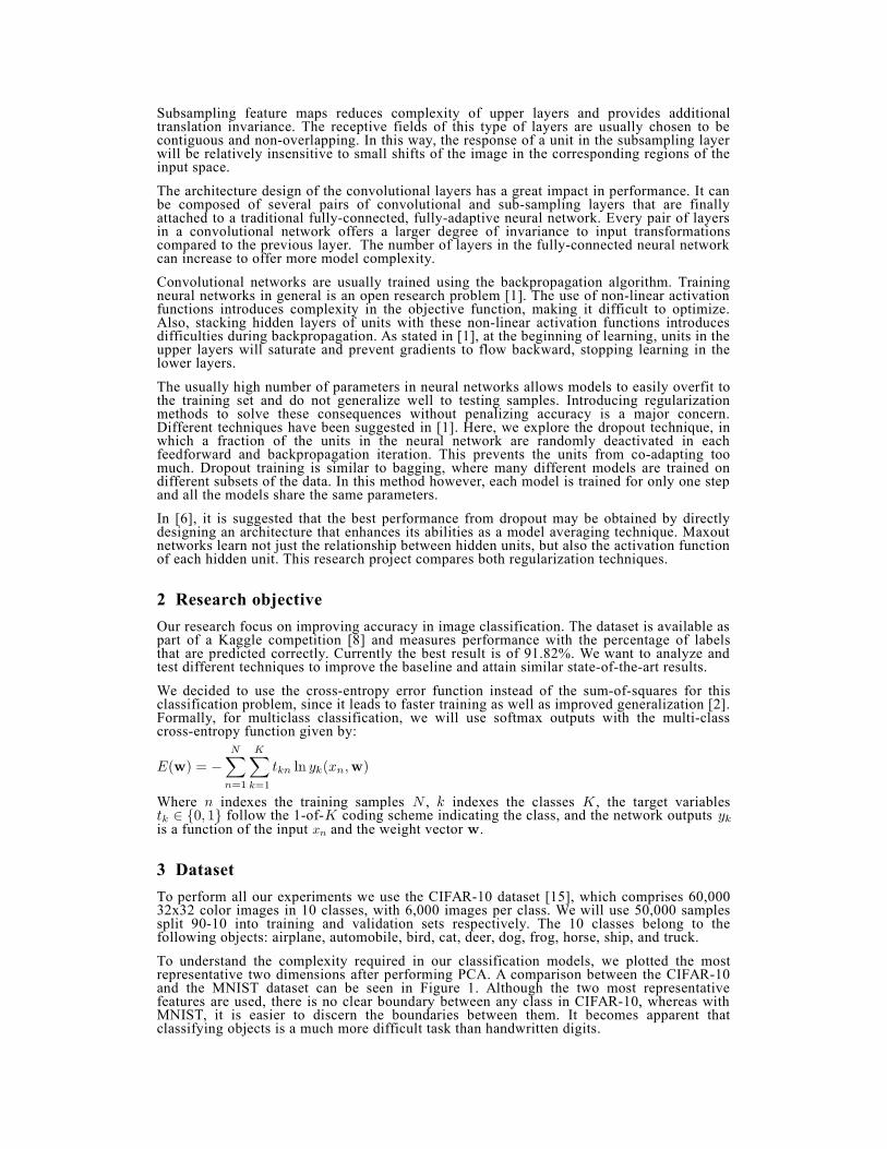
To understand the complexity required in our classification models, we plotted the mostrepresentative two dimensions after performing PCA. A comparison between the CIFAR-10and the MNIST dataset can be seen in Figure 1. Although the two most representativefeatures are used, there is no clear boundary between any class in CIFAR-10, whereas withMNIST, it is easier to discern the boundaries between them. It becomes apparent thatclassifying objects is a much more difficult task than handwritten digits.

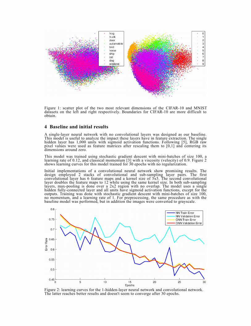
Figure 1: scatter plot of the two most relevant dimensions of the CIFAR-10 and MNISTdatasets on the left and right respectively. Boundaries for CIFAR-10 are more difficult toobtain.

4 Baseline and initial results

A single-layer neural network with no convolutional layers was designed as our baseline.This model is useful to analyze the impact these layers have in feature extraction. The singlehidden layer has 1,000 units with sigmoid activation functions. Following [5], RGB rawpixel values were used as feature matrices after rescaling them to [0,1] and centering itsdimensions around zero.

This model was trained using stochastic gradient descent with mini-batches of size 100, alearning rate of 0.12, and classical momentum [3] with a viscosity (velocity) of 0.9. Figure 2shows learning curves for this model trained for 30 epochs with no regularization.

Initial implementations of a convolutional neural network show promising results. Thedesign employed 2 stacks of convolutional and sub-sampling layer pairs. The firstconvolutional layer has 6 feature maps and a kernel size of 5x5. The second convolutionallayer doubles the feature maps to 12 while using the same kernel size. In both sub-samplinglayers, max-pooling is done over a 2x2 region with no overlap. The model uses a singlehidden fully-connected layer and all units have sigmoid activation functions, except for theoutputs. Training was done with stochastic gradient descent with mini-batches of size 100,no momentum, and a learning rate of 1. For preprocessing, the same procedure as with thebaseline model was performed, but in addition the images were converted to grayscale.

Figure 2: learning curves for the 1-hidden-layer neural network and convolutional network.The latter reaches better results and doesn't seem to converge after 30 epochs.

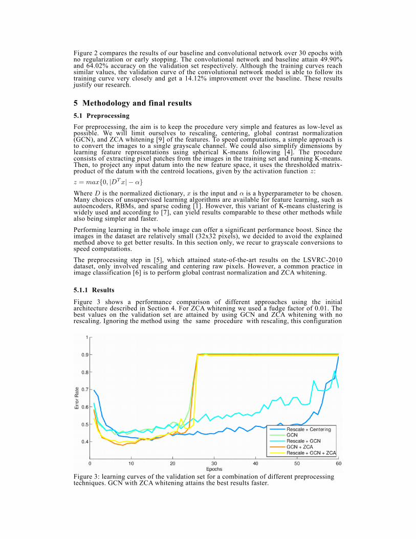
Figure 2 compares the results of our baseline and convolutional network over 30 epochs withno regularization or early stopping. The convolutional network and baseline attain 49.90%and 64.02% accuracy on the validation set respectively. Although the training curves reachsimilar values, the validation curve of the convolutional network model is able to follow itstraining curve very closely and get a 14.12% improvement over the baseline. These resultsjustify our research.

5 Methodology and final results

5.1 Preprocessing

For preprocessing, the aim is to keep the procedure very simple and features as low-level aspossible. We will limit ourselves to rescaling, centering, global contrast normalization(GCN), and ZCA whitening [9] of the features. To speed computations, a simple approach isto convert the images to a single grayscale channel. We could also simplify dimensions bylearning feature representations using spherical K-means following [4]. The procedureconsists of extracting pixel patches from the images in the training set and running K-means.Then, to project any input datum into the new feature space, it uses the thresholded matrix-product of the datum with the centroid locations, given by the activation function :

Where is the normalized dictionary, is the input and is a hyperparameter to be chosen.Many choices of unsupervised learning algorithms are available for feature learning, such asautoencoders, RBMs, and sparse coding [1]. However, this variant of K-means clustering iswidely used and according to [7], can yield results comparable to these other methods whilealso being simpler and faster.

Performing learning in the whole image can offer a significant performance boost. Since theimages in the dataset are relatively small (32x32 pixels), we decided to avoid the explainedmethod above to get better results. In this section only, we recur to grayscale conversions tospeed computations.

The preprocessing step in [5], which attained state-of-the-art results on the LSVRC-2010dataset, only involved rescaling and centering raw pixels. However, a common practice inimage classification [6] is to perform global contrast normalization and ZCA whitening.

5.1.1 Results

Figure 3 shows a performance comparison of different approaches using the initialarchitecture described in Section 4. For ZCA whitening we used a fudge factor of 0.01. Thebest values on the validation set are attained by using GCN and ZCA whitening with norescaling. Ignoring the method using the same procedure with rescaling, this configuration

Figure 3: learning curves of the validation set for a combination of different preprocessingtechniques. GCN with ZCA whitening attains the best results faster.

yields a 2.88% improvement over the next one and is also the fastest. After several iterationsthe training errors go up presumably because of a slightly high learning rate. Furtherexperiments will only use this preprocessing technique.

5.2 Implementation

Although we relied on our own implementation to develop our baseline results andpreprocessing benchmarks, it wasn't really capable of taking advantage of parallelcomputations through GPUs. If our intention is to achieve state-of-the-art results we need todesign bigger neural networks with many more parameters than the previous models. Fordropout to work well, it also requires highly parametrized models that can easily overfit thedata.

Training a model under such conditions would take an immense amount of time on CPUs.Therefor, we made extensive use of Pylearn2 [13], a machine learning framework developedin Python. It builds on top of Theano [14], a numerical computation library that compiles torun efficiently on GPU architectures such as CUDA.

We had at our disposition 8 Nvidia Tesla Fermi M2090 cGPUs, with 6GB of RAM each,providing enough memory to fit our largest neural network. The application server usesversion 4.3 of the CUDA libraries. With this set-up, training our largest model took 2 days.

5.3 Activation units

Units using sigmoid or tanh functions have been known for saturating easily during training,preventing gradients to flow back to other layers. Even though convolutional layers have areduced number of units due to parameter sharing, our aim is to introduce a considerablenumber of these layers combined with multiple dense, fully-connected layers. With thisconfiguration, it is thought sigmoid functions will perform poorly. The recently suggestedRectified Linear Units (ReLUs), a non-saturating function given by , seem totrain several times faster in [5].

5.3.1 Results

Figure 4 shows a comparison between the three types of units using a deep model verysimilar to [5], involving a convolutional-pooling pair layer followed by two successiveconvolutional layers, a max-pooling layer plus two dense hidden layers. ReLUs are faster,and they seem to reach better results for the small number of epochs used. The use of ReLUsin all following experiments is justified.

Figure 4: learning curves of the validation set for CNN models using units with ReLU, tanhand sigmoid activation functions.

5.4 Training

In the aims of providing a fair comparison between the models and regularization techniquesbeing presented, the same training schedule and hyperparameters were used for allexperiments. Optimization is addressed by using Nesterov's accelerated gradient with mini-batches [3]. The viscosity (velocity) and weight updates are given by:

Where is the learning rate, is the momentum coefficient, and is thegradient of the parameters at time . It is common [5, 10] to use a fixed momentum of 0.9, orto initialize it at 0.5 and increase it gradually during the first 10-20 epochs until 0.9.

We found out that after increasing momentum to values close to 0.7, the negative log-likelihood in our maxout networks starts going up until it reaches intolerable values. Thenoise provided by dropout and maxout networks allows the training algorithm to exploredifferent regions of the objective function with a large learning rate [6, 12]. Momentumintroduces a weighted direction based on the history of previous steps. Setting a large weightfor that direction in this chaotic environment seems to be affecting maxout units negatively.Even in dropout, although the model is still able to learn, better results were attained with alower momentum. It seems that the same learning rate gives maxout networks a moreoscillatory behavior than dropout networks. Hence, best results were attained whenmomentum was initialized to 0.5 and linearly increased until 0.6 after 250 epochs. Thisconfiguration will be used with the two regularization techniques.

As per our discussion, a sufficiently large learning rate of 0.17 was chosen to allowexploration of the objective function. To enforce the learning algorithm to eventually settlefor a path and exploit it, we implement a linear decay of the learning rate, saturating in 500epochs with a factor of 0.01 the original value. Since feature maps in convolutional networksshare weights across different regions and see more training examples in an iteration, theirweights should take smaller steps towards the gradient to prevent overfitting. Therefore,during training, gradients of the weights and biases in convolutional layers are scaled downto 0.05 times the global learning rate.

Although dropout and maxout act as powerful regularizers, they can't prevent the weightsfrom reaching computational intractable values. We apply constrains to the weights by usingthe max-norm regularization [12], in which . In convolutional layers representsthe weights of kernel , whereas in a full-connected layer, is a vector of the weightsincident on hidden unit . The hyperparameter was set to , initially in all instances.However, a few models were still having overflow issues because of the weights in the firstlayer. Setting for the set of kernel weights in that layer fixed the problem.

Weight initialization is even more crucial for dropout than maxout networks. Initialconfigurations got learning stuck in local minima for almost every model, requiring us toincrease the range of the interval. After better settings were found, faster learning in the firstiterations was attained by setting different sampling ranges according to the type of layer.Convolutional layers are more sensible to initialization and require a wider sampling range.We initialize their pertaining weights to , where function denotes the range ofa uniform continuous distribution. Once there, initial training is faster if fully-connectedlayers are initialized with . Biases are initialized to 0.

Finally, we trained with mini-batches of size 100 and early stopping was used to aborttraining if the validation error does not improve for a good amount of epochs. The previous20 misclassification errors on the validation set are kept. The algorithm will stop when theearliest value is the lowest in the set, returning the best version of the neural network found.There was no cap on the number of epochs.

5.5 Architectures

We experiment with different network architectures and study their impact on theclassification task. There are many possible configurations but not many work well. Asstated in [10], adding feature detectors increases the number of parameters and althoughadding pooling layers reduces the number of nodes in the next layer and introducesinvariance, successive subsampling operations lose information about the position of thefeatures in the image. As it was also stated in [10], pooling the maximum value (max-pooling) instead of the average usually works better in practice.

Taking in consideration these suggestions and observing other successful architectures, wedecided to implement 4 models similar to those in LeNet-5 [11], deep convolutional neural

networks [5], dropout in convolutional networks as in [12], and maxout networks [6]. Themodels are described as follows:

• Model 1: this model follows LeNet-5, but scales up the number of feature maps insimilar proportions. It starts with 64 5x5 feature maps max-pooled to 2x2 with nooverlap, followed by a convolutional layer of 96 5x5 feature maps using the samesubsampling configuration. The following convolutional layer extracts 160 5x5feature maps with no pooling. Unlike The original LeNet-5 [11], our single denselayer has 1,000 units. This model is characterized by an increasing number offeature maps of the same kernel size in each successive convolutional layer.

• Model 2: similar to [10] but reduces the kernel and pool sizes to accommodate forthe lack of padding, this model has 3 convolutional layers with max-pooling. Thefirst and second layer have 96 and 192 feature maps respectively with 5x5 kernelsand a pooling region of 3x3 with a stride of 2, allowing for overlap. The thirdconvolutional layer has 192 feature maps with 3x3 kernels and a 2x2 pooling regionwith the same stride 2 (no overlap). The model has only one fully-connected layerwith 500 units. It explores having layers with large number of feature maps but withbig pooling windows that effectively reduce the number of parameters in the upperlayers.

• Model 3: the convolutional layers in this model are less parametrized than Model 2and have a similar distribution of feature maps as Model 1. We incorporateoverlapping pooling and add two large fully-connected hidden layers. The model isvery similar to [12] but the size of the pooling window are reduced in the first layerto account for the lack of padding. The three convolutional layers have 5x5 kernelswith 64, 64 and 128 feature maps respectively. The first layer has a 2x2 pool shapewith a stride of 1. Same as Model 2, layers 2 and 3 have a pooling region of 3x3with a stride of 2. The following two dense layers have 3,072 and 2,048 units, inorder, from input to output. This model explores the impact of having a deep andlarge fully-connected neural network in the upper layers.

• Model 4: follows a similar architecture to that in [5] used for CIFAR-100. Since thedataset used here has less classes and the input images are smaller, the number ofparameters is downscaled for each layer. The model has 5 convolutional layers and 2fully-connected. The connections between convolutional layers 3-4 and 4-5 are notsubsampled. Connections between 1-2, 2-3 and 5-6 are max-pooled with a region of2x2 and a stride of 1, allowing again for some overlapping. As we stackconvolutional layers we decrease the size of the kernels. Going from convolutionallayers to fully connected layers, the number of feature maps are 32, 48, 64, 64, 48,and the kernel shapes are 8x8, 5x5, 3x3, 3x3, 3x3. The dense layers have 500 unitseach. This model explores depth in the number of layers. We reduced the number ofparameters to make it comparable to other models. Even though it has 5convolutional layers, supsampling is only performed 3 times as it goes up thenetwork.

As empirically observed in [5], models with overlapping pooling are more difficult tooverfit. All kernels have a stride of 1 so patches overlap as much as possible. Also, allmodels except Model 1 perform subsampling three times across the network. Only Model 1does perform subsampling twice and so it retains more spatial information about the detectedfeatures in the image. All models use ReLUs and biases in the convolutional layers areshared across RGB channels.

5.5.1 Results

Figure 5 compares the performance of the 4 models, all trained under the same conditionspresented in Section 5.4. The best learning curve belongs to Model 3 without maxout,achieving a 16.55% error rate on the validation set, though the best value is attained byModel 2 with maxout, with 16.26%. Model 4 obtains the worst performance with 22.97%.

Because of the performance obtained with Model 4, it can be said that depth is not such animportant factor in obtaining good accuracy. Also, the fewer subsampling layers in Model 1intended to retain spatial information, are not essential for performance.

Model 2 and Model 3 seem to represent the most reasonable architectures, suggesting thatthe number of parameters dominates performance. Model 2 has a lot of parameters (featuremaps) in the convolutional layers while Model 3 has fewer feature maps, but adds an extrafully-connected layer with a higher number of units. Although the pooling windows in thefirst layer of Model 3 are smaller (2x2 with a stride of 1), the difference is not asconsiderable as the distribution of parameters between the convolutional and the fully-

connected layers. Model 3 attained similar performance with considerably less feature mapsjust by adding a large fully-connected layer.

5.6 Regularization

In dropout [12], the choice of which units to drop is random. In the simplest case, all unitsare retained with a fixed probability. This probability is sampled independently for eachhidden unit and for each training case. Since every configuration of activated unitsrepresents a different model, the predictions have to be averaged at test time. We couldsample predictions using dropout and average the results by the number of models seen butthis may require many samples to minimize error. An average approximation that does notrequire sampling and works well in practice multiplies the outgoing weights of that unit withits probability of being retained.

In our experiments, we could have explored different probability settings for different layersbut we decided to use a common approach [12] where the probability of retaining units in thefirst layers is higher. Thus, the models have 0.8 probability for the input layer and 0.5 for thelayers in the rest of the network.

From our discussion in 1.4, maxout networks introduces an activation function given by:

Where is the inner product of the input of the layer and the weight vector plussome bias :

Unlike conventional neural networks where the activation function is applied to each ,maxout networks group together units of and take the maximum. In a convolutionallayer, a maxout feature map can be constructed by grouping affine feature maps, usually,and as it is the case in our experiments, by channel and region. Following [6], a singlemaxout unit can be interpreted as making a piecewise linear approximation to an arbitraryconvex function.

Different grouping schemes are employed depending on the type of layer. Convolutionallayers use 2 linear pieces ( ) for a maxout unit and hidden layers use 5. These groups havestrides equal to the number of pieces, which makes them disjoint. Maxout networks areconsidered a natural companion to dropout [6] and our experiments use the same dropoutconfiguration explained above.

Figure 5: learning curves of the validation set for the four CNN models, trained underdropout and maxout with dropout.

5.6.1 Results

Shown in Figure 5, maxout improves the accuracy of Models 1 and 2 by 2.21% and 0.40%respectively, whereas Model 3 is considerably worse. Model 4 is halted by the early stoppingalgorithm in multiple runs but the curve is always above the dropout counterpart.

Although not shown in Figure 5, the gap between the training and validation curves withmaxout seem to be smaller. Also, the learning curves in Models 3 and 4 have manyoscillations. Both observations suggest that maxout is a stronger regularizer and introducesmore noise than just using dropout. We hypothesize that the additional fully-connected layerin models 3 and 4 generates a more complex objective surface that the maxout method is notable to properly optimize because it is introducing too much noise. A solution could be toreduce the learning rate or make clusters assigned to maxout units in the fully-connectedlayers smaller. The current selected number of pieces for these layers was 5, it may havebeen set too high.

A hypothesis on why maxout may be a better architecture is that it better propagatesinformation to the lower layers [6]. Even when a maxout unit is 0, the gradient informationstill flows to the parameters of the function, its units. Another reason entertained in [6] isthat the max-pooling operation in convolutional layers fits more naturally as a part ofmaxout.

6 Conclusions

We laid down the foundations for our research and initial results showed that the endeavorwas worth exploring. Indeed, convolutional neural networks are able to outperform fully-connected neural networks of similar complexity by learning invariant feature detectors. Aswe have also seen, ReLUs train much faster than tanh units and in the case of sigmoid unitsin can attain better results by avoiding saturation.

Although we cannot guarantee our preprocessing results can generalize to other datasets, wefound that best results are obtained in CIFAR-10 when using GCN with ZCA whitening. Wethen designed and tested different models exploring different directions and found out thatwe attain better results by increasing the number of parameters over depth. The number ofunits in the fully-connected layers has as much impact as adding feature maps.

Maxout introduces more noise during training that can benefit accuracy. As complexityincreases though, it can have a negative impact that can potentially be solved by usingdifferent training hyperparameters or more sparse maxout units. Our experiments imply thatthe method can't guarantee performance boosts in all situations.

There are many additional ideas we can explore to attain state-of-the-art results. First,padding the input image and the feature maps allows for better detection of features that maylie on the borders. Current state-of-the-art approaches seem to rely on this [5, 6].

Data augmentation techniques can reduce overfitting by artificially generating new trainingexamples from the existent dataset [5]. These new examples posses some variance we hopethe inference algorithm is able to account for. Some label-preserving transformations consistof generating image translations and horizontal reflections. A similar idea to padding wouldbe to extract smaller patches of the image with random offsets. Altering the intensities of theRGB channels makes the learning algorithm invariant to small changes in color andillumination. This idea could be a more powerful alternative than preprocessing images withcontrast normalization and whitening.

Lastly, it would be interesting to study the impact of different dropout and maxoutconfigurations. We could, for instance, assign a higher probability of retaining units toconvolutional layers and not just the inputs [5]. In maxout networks, the number of piecesper maxout unit can have a drastic impact in the complexity of the model that is worthstudying.

Acknowledgments

We thank professor Brendan Frey for teaching many of the concepts involved in this project,the Department of Computer Science at University of Toronto for making their hardware andapplication servers available, and the Pylearn2 [13] and Theano [14] teams, whose blazinglyfast algorithm implementations made computations feasible.

References

[1] Glorot, X., and Bengio Y. Understanding the difficulty of training deep feedforward neuralnetworks. In AISTATS, 2010.

[2] Simard, P. Y., D. Steinkraus, and J. Platt (2003). Best practices for convolutional neural networksapplied to visual document analysis. In Proceedings International Conference on Document Analysisand Recognition (ICDAR), 2003.

[3] Sutskever I., Martens J., Dahl G., and Hinton G. On the importance of initialization andmomentum in deep learning. In ICML, 2013.

[4] Coates A., and Ng. A., Learning Feature Representations with K-means. In Neural Networks:Tricks of the Trade, Reloaded, 2012.

[5] Krizhevsky A., Sutskever I., and Hinton, G. Imagenet classification with deep convolutional neuralnetworks. In Advances in Neural Information Processing Systems 25 , 2012.

[6] Goodfellow, I., Warde-Farley, D., Mirza, M., Courville, A., and Bengio, Y. (2013b). Maxoutnetworks. In ICML, 2013.

[7] Coates A., Carpenter B., Case C., Satheesh S., Suresh B., Wang T., Wu D. J., and Ng A.. Textdetection and character recognition in scene images with unsupervised feature learning. In ICDAR,2011.

[8] Krizhevsky, A. Learning Multiple Layers of Features from Tiny Images. http://www.kaggle.com/c/cifar-10 , 2009.

[9] Hyvarinen A., and Oja E. Independent component analysis: algorithms and applications. In Neuralnetworks, 2000.

[10] Hinton, G. Neural Networks for Machine Learning. http://www.coursera.org/course/neuralnets , 2012.

[11] LeCun Y., et al. Gradient-based learning applied to document recognition, In Proceedings of theIEEE, 1998.

[12] Srivastava, N. Improving neural networks with dropout. Master's thesis, University of Toronto,2013.

[13] Goodfellow I., Warde-Farley D., Lamblin P., Dumoulin V., Mirza M., Pascanu R., Bergstra J.,Bastien F., and Bengio Y. Pylearn2: a machine learning research library. arXiv preprintarXiv:1308.4214

[14] Bergstra J., Breuleux O., Bastien F., Lamblin P., Pascanu R., Desjardins G., Turian J., Warde-Farley D., and Bengio Y. Theano: A CPU and GPU Math Expression Compiler. In Proceedings of thePython for Scientific Computing Conference, 2010.

[15] Krizhevsky A.Learning Multiple Layers of Features from Tiny Images. http://www.cs.toronto.edu/~kriz/learning-features-2009-TR.pdf , 2009.