best practice ead modelling methodologies v1.4

Best Practice EAD Modelling

MethodologiesCredit Modelling Forum, Sydney

14th Dec 2015

1

Copyright © 2015 Accenture All rights reserved.2

Background

Defining and Allocating EAD

EAD Ratios

Observation Definitions

EAD Drivers

Maximising Discrimination Using Nested Models

EAD Calibration

IFRS 9 Impairment Methodology

CONTENTS

1

2

3

4

5

6

7

8

BACKGROUND


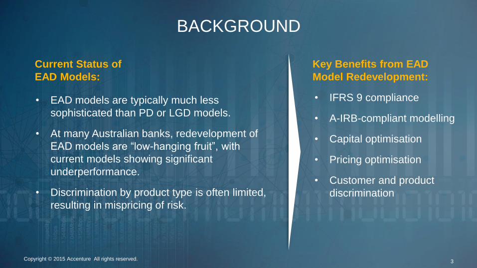
• EAD models are typically much less

sophisticated than PD or LGD models.

• At many Australian banks, redevelopment of

EAD models are “low-hanging fruit”, with

current models showing significant

underperformance.

• Discrimination by product type is often limited,

resulting in mispricing of risk.

• IFRS 9 compliance

• A-IRB-compliant modelling

• Capital optimisation

• Pricing optimisation

• Customer and product

discrimination

Current Status of

EAD Models:

Key Benefits from EAD

Model Redevelopment:

DEFINING EAD

0

1

2

3

4

5

6

7

8

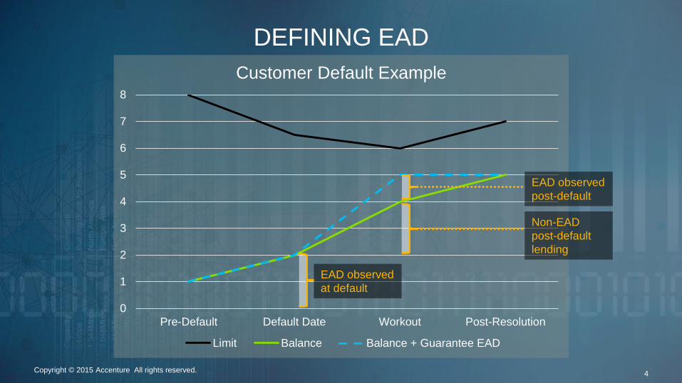
Pre-Default Default Date Workout Post-Resolution

Customer Default Example

Limit Balance Balance + Guarantee EAD

EAD observed

at default

EAD observed

post-default

Non-EAD

post-default

lending


DEFINING EAD


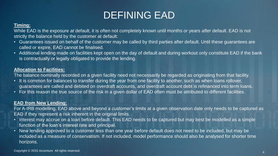
Timing:

While EAD is the exposure at default, it is often not completely known until months or years after default. EAD is not

strictly the balance held by the customer at default:

• Guarantees issued on behalf of the customer may be called by third parties after default. Until these guarantees are

called or expire, EAD cannot be finalised.

• Additional lending made on facilities kept open on the day of default and during workout only constitute EAD if the bank

is contractually or legally obligated to provide the lending.

Allocation to Facilities:

The balance nominally recorded on a given facility need not necessarily be regarded as originating from that facility.

• It is common for balances to transfer during the year from one facility to another, such as when loans rollover,

guarantees are called and debited on overdraft accounts, and overdraft account debt is refinanced into term loans.

• For this reason the true source of the risk in a given dollar of EAD often must be attributed to different facilities.

EAD from New Lending:

For A-IRB modelling, EAD above and beyond a customer’s limits at a given observation date only needs to be captured as

EAD if they represent a risk inherent in the original limits.

• Interest may accrue on a loan before default. This EAD needs to be captured but may best be modelled as a simple

function of the loan’s interest rate and principal.

• New lending approved to a customer less than one year before default does not need to be included, but may be

included as a measure of conservatism. If not included, model performance should also be analysed for shorter time

horizons.

ALLOCATION OF EAD

0

2

4

6

8

10

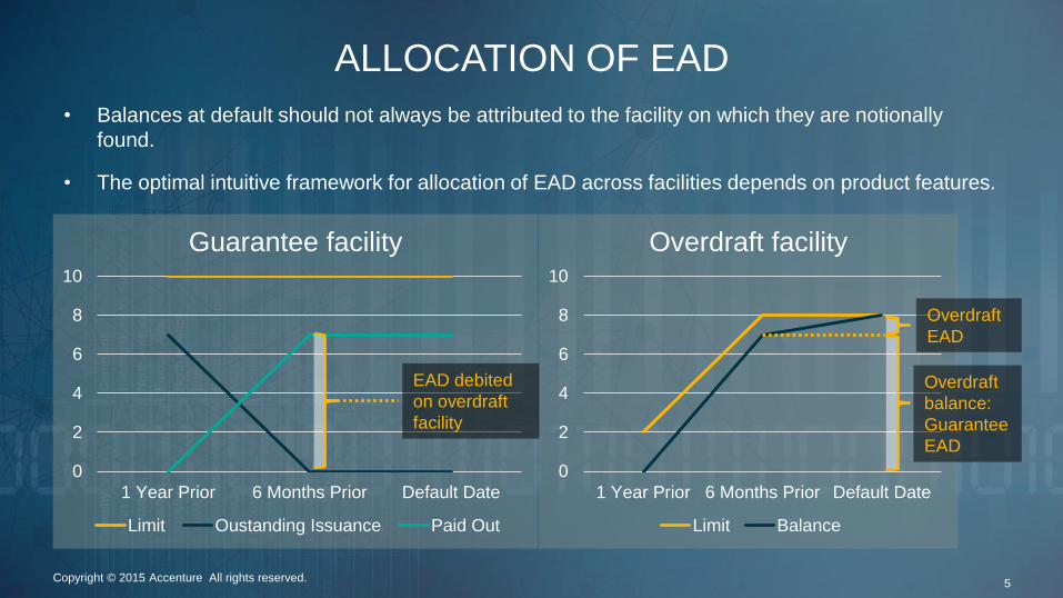
1 Year Prior 6 Months Prior Default Date

Guarantee facility

Limit Oustanding Issuance Paid Out

EAD debited

on overdraft

facility

0

2

4

6

8

10

1 Year Prior 6 Months Prior Default Date

Overdraft facility

Limit Balance

Overdraft

balance:

Guarantee

EAD

Overdraft

EAD

• Balances at default should not always be attributed to the facility on which they are notionally

found.

• The optimal intuitive framework for allocation of EAD across facilities depends on product features.


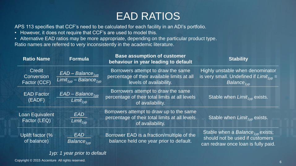
EAD RATIOS

Ratio Name FormulaBase assumption of customer

behaviour in year leading to defaultStability

Credit

Conversion

Factor (CCF)

EAD – Balance1yp

Limit1yp – Balance1yp

Borrowers attempt to draw the same

percentage of their available limits at all

levels of availability.

Highly unstable when denominator

is very small. Undefined if Limit1yp =

Balance1yp

EAD Factor

(EADF)

EAD – Balance1yp

Limit1yp

Borrowers attempt to draw the same

percentage of their total limits at all levels

of availability.

Stable when Limit1yp exists.

Loan Equivalent

Factor (LEQ)

EAD

Limit1yp

Borrowers attempt to draw up to the same

percentage of their total limits at all levels

of availability.

Stable when Limit1yp exists.

Uplift factor (%

of balance)

EAD

Balance1yp

Borrower EAD is a fraction/multiple of the

balance held one year prior to default.

Stable when a Balance1yp exists;

should not be used if customers

can redraw once loan is fully paid.

1yp: 1 year prior to default


APS 113 specifies that CCF’s need to be calculated for each facility in an ADI’s portfolio.

• However, it does not require that CCF’s are used to model this.

• Alternative EAD ratios may be more appropriate, depending on the particular product type.

Ratio names are referred to very inconsistently in the academic literature.

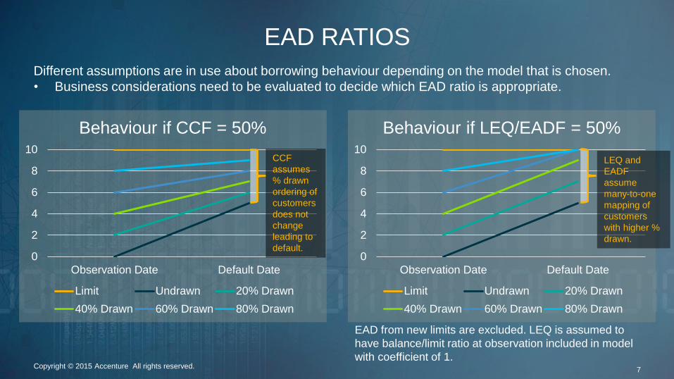
EAD RATIOS

EAD from new limits are excluded. LEQ is assumed to

have balance/limit ratio at observation included in model

with coefficient of 1.

Different assumptions are in use about borrowing behaviour depending on the model that is chosen.

• Business considerations need to be evaluated to decide which EAD ratio is appropriate.

0

2

4

6

8

10

Observation Date Default Date

Behaviour if CCF = 50%

Limit Undrawn 20% Drawn

40% Drawn 60% Drawn 80% Drawn

0

2

4

6

8

10

Observation Date Default Date

Behaviour if LEQ/EADF = 50%

Limit Undrawn 20% Drawn

40% Drawn 60% Drawn 80% Drawn


CCF

assumes

% drawn

ordering of

customers

does not

change

leading to

default.

LEQ and

EADF

assume

many-to-one

mapping of

customers

with higher %

drawn.

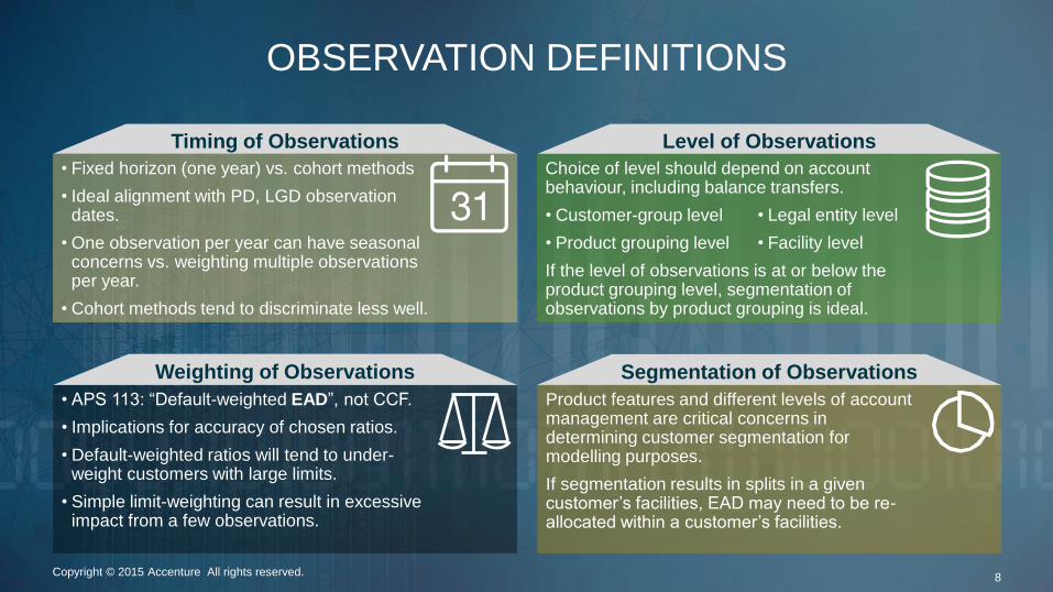
OBSERVATION DEFINITIONS

• Fixed horizon (one year) vs. cohort methods

• Ideal alignment with PD, LGD observation dates.

• One observation per year can have seasonal concerns vs. weighting multiple observations per year.

• Cohort methods tend to discriminate less well.

Choice of level should depend on account behaviour, including balance transfers.

• Customer-group level

• Product grouping level

If the level of observations is at or below the product grouping level, segmentation of observations by product grouping is ideal.

• APS 113: “Default-weighted EAD”, not CCF.

• Implications for accuracy of chosen ratios.

• Default-weighted ratios will tend to under-weight customers with large limits.

• Simple limit-weighting can result in excessive impact from a few observations.

Product features and different levels of account management are critical concerns in determining customer segmentation for modelling purposes.

If segmentation results in splits in a given customer’s facilities, EAD may need to be re-allocated within a customer’s facilities.

Segmentation of Observations

Level of ObservationsTiming of Observations

Weighting of Observations

• Legal entity level

• Facility level


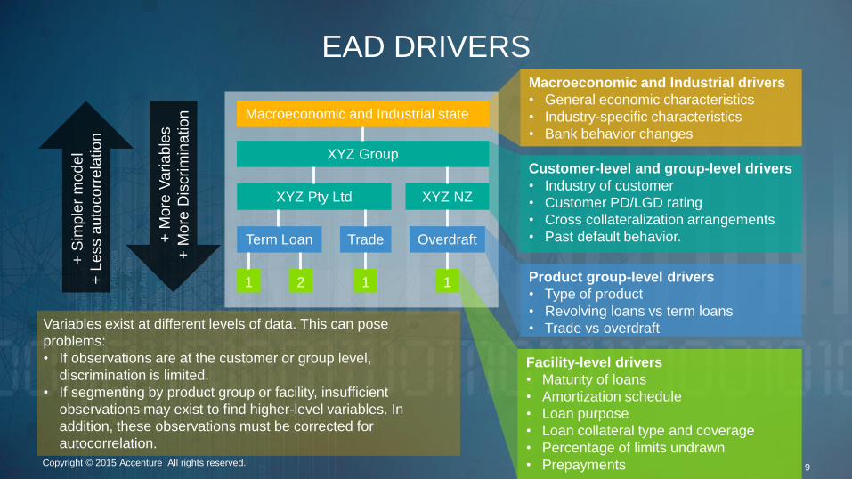
EAD DRIVERS

Customer-level and group-level drivers

• Industry of customer

• Customer PD/LGD rating

• Cross collateralization arrangements

• Past default behavior.

Facility-level drivers

• Maturity of loans

• Amortization schedule

• Loan purpose

• Loan collateral type and coverage

• Percentage of limits undrawn

• Prepayments

Product group-level drivers

• Type of product

• Revolving loans vs term loans

• Trade vs overdraft

Macroeconomic and Industrial drivers

• General economic characteristics

• Industry-specific characteristics

• Bank behavior changes

1

Term Loan

Macroeconomic and Industrial state

XYZ Pty Ltd

Trade

2 1

XYZ Group

XYZ NZ

Overdraft

1

+ S

imple

r m

odel

+ L

ess a

uto

corr

ela

tion

+ M

ore

Variable

s

+ M

ore

Dis

crim

ination

Variables exist at different levels of data. This can pose

problems:

• If observations are at the customer or group level,

discrimination is limited.

• If segmenting by product group or facility, insufficient

observations may exist to find higher-level variables. In

addition, these observations must be corrected for

autocorrelation.


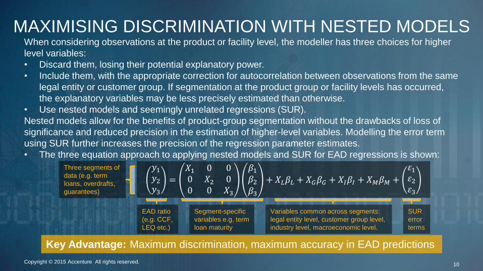
MAXIMISING DISCRIMINATION WITH NESTED MODELSWhen considering observations at the product or facility level, the modeller has three choices for higher

level variables:

• Discard them, losing their potential explanatory power.

• Include them, with the appropriate correction for autocorrelation between observations from the same

legal entity or customer group. If segmentation at the product group or facility levels has occurred,

the explanatory variables may be less precisely estimated than otherwise.

• Use nested models and seemingly unrelated regressions (SUR).

Nested models allow for the benefits of product-group segmentation without the drawbacks of loss of

significance and reduced precision in the estimation of higher-level variables. Modelling the error term

using SUR further increases the precision of the regression parameter estimates.

• The three equation approach to applying nested models and SUR for EAD regressions is shown:

Key Advantage: Maximum discrimination, maximum accuracy in EAD predictions


𝑦1𝑦2𝑦3

=𝑋1 0 00 𝑋2 00 0 𝑋3

𝛽1𝛽2𝛽3

+ 𝑋𝐿𝛽𝐿 + 𝑋𝐺𝛽𝐺 + 𝑋𝐼𝛽𝐼 + 𝑋𝑀𝛽𝑀 +

𝜀1𝜀2𝜀3

EAD ratio

(e.g. CCF,

LEQ etc.)

Three segments of

data (e.g. term

loans, overdrafts,

guarantees)

Segment-specific

variables e.g. term

loan maturity

Variables common across segments:

legal entity level, customer group level,

industry level, macroeconomic level.

SUR

error

terms

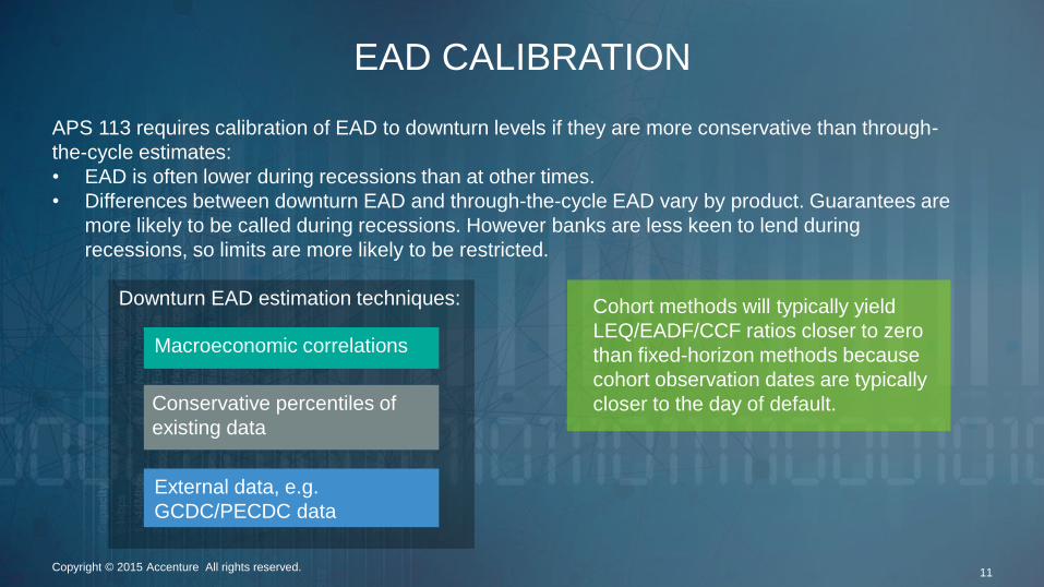
Downturn EAD estimation techniques:

EAD CALIBRATION

APS 113 requires calibration of EAD to downturn levels if they are more conservative than through-

the-cycle estimates:

• EAD is often lower during recessions than at other times.

• Differences between downturn EAD and through-the-cycle EAD vary by product. Guarantees are

more likely to be called during recessions. However banks are less keen to lend during

recessions, so limits are more likely to be restricted.

Cohort methods will typically yield

LEQ/EADF/CCF ratios closer to zero

than fixed-horizon methods because

cohort observation dates are typically

closer to the day of default.

Macroeconomic correlations

External data, e.g.

GCDC/PECDC data

Conservative percentiles of

existing data


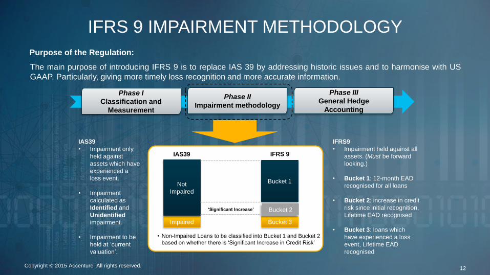
IFRS 9 IMPAIRMENT METHODOLOGY

Purpose of the Regulation:

The main purpose of introducing IFRS 9 is to replace IAS 39 by addressing historic issues and to harmonise with US

GAAP. Particularly, giving more timely loss recognition and more accurate information.

Phase II

Impairment methodology

Phase I

Classification and

Measurement

Phase III

General Hedge

Accounting

IAS39

• Impairment only

held against

assets which have

experienced a

loss event.

• Impairment

calculated as

Identified and

Unidentified

impairment.

• Impairment to be

held at ‘current

valuation’.

IFRS9

• Impairment held against all

assets. (Must be forward

looking.)

• Bucket 1: 12-month EAD

recognised for all loans

• Bucket 2: increase in credit

risk since initial recognition,

Lifetime EAD recognised

• Bucket 3: loans which

have experienced a loss

event, Lifetime EAD

recognised

Impaired

Not

Impaired

Bucket 3

Bucket 1

Bucket 2

IAS39 IFRS 9

• Non-Impaired Loans to be classified into Bucket 1 and Bucket 2

based on whether there is ‘Significant Increase in Credit Risk’

‘Significant Increase’


Identify

Portfolio and Data

− Identify portfolio,

exposures and

sub-segments

− Gather internal

data on the

portfolio is

compiled (e.g.

performance data)

− Analyze bank

master scale with

historical data

− Analyze existing

process, models

and

methodologies,

e.g., point-in-time

adjustments,

existing rating

distributions, model

inventory, etc.

Classify

Exposure

− Classify exposure

into three Buckets:

• Bucket 1:

performing assets

• Bucket 2: Credit

Risk is increased

significantly

• Bucket 3: Credit

Losses are

incurred

− Define ‘significant

increase in credit

risk’

• Quantify PD

deterioration, if

available

• Internal watch list

• Delinquency info

• Consider forward

looking factors

Develop Dual

Calibration

− Select appropriate

calibration

methodology

based on portfolio,

model type, data

availability, etc.

− TTC and PiT

methodologies:

• Default Distance

(DD) method

• Adjustment

scalar factor

method

− Test convergence

to central tendency

Quantify

Expected Loss

Monitoring and

Reporting

− Define and design

method for

Expected Credit

Loss aggregation

− Identify KPIs for

reporting

dashboards for

business, audit,

and regulators

− Develop executive

dashboards for

IFRS 9 reporting

− Automate model

monitoring to re-

classify the

exposures on

frequent basis

Banks are challenged to comply with both IFRS9 and Basel norms given the differences in the underlying

rating philosophy implied – PiT for IFRS 9 and TTC for Basel. A

cti

vit

ies

1 2 3 4 5

− Lifetime EL

Methodologies

• Migration

Matrices

approach or roll

rate models

• Survival Analysis

• Regression

Model Based

• LGD x EAD

methods

− Impact by

exposure

classification,

discount rates,

modeling choice

− Review with

stakeholders

− Socialize within

bank to get buy-in


IFRS 9 IMPAIRMENT METHODOLOGY

THANK YOU

Questions?

14

David OngAnalytics Manager

Accenture Digital

[email protected]

Melbourne, Australia

Curtis ErikssonAnalytics Senior Manager

Accenture Digital

[email protected]

Sydney, Australia

Follow Accenture Analytics on Twitter:

@ISpeakAnalytics

Copyright © 2015 Accenture All rights reserved.

best practice ead modelling methodologies v1.4

Documents