w o r k i n g

p a p e r

F E D E R A L R E S E R V E B A N K O F C L E V E L A N D

21 11

Export-Led Decay: The Trade Channel in the Gold Standard Era

Bernardo Candia and Mathieu Pedemonte

ISSN: 2573-7953

Working papers of the Federal Reserve Bank of Cleveland are preliminary materials circulated to stimulate discussion and critical comment on research in progress. They may not have been subject to the formal editorial review accorded official Federal Reserve Bank of Cleveland publications. The views expressed herein are solely those of the authors and do not necessarily reflect the views of the Federal Reserve Bank of Cleveland or the Board of Governors of the Federal Reserve System.

Working papers are available on the Cleveland Fed’s website at:

www.clevelandfed.org/research.

Working Paper 21-11 May 2021

Export-Led Decay: The Trade Channel in the Gold Standard EraBernardo Candia and Mathieu Pedemonte

Flexible exchange rates can facilitate price adjustments that buffer macroeconomic shocks. We test this hypothesis using adjustments to the gold standard during the Great Depression. Using prices at the goods level, we estimate exchange rate pass-through and find gains in competitiveness after a depreciation. Using novel monthly data on city-level economic activity, combined with employment composition and sectoral export data, we show that American exporting cities were significantly affected by changes in bilateral exchange rates. They were negatively impacted when the UK abandoned the gold standard in 1931 and benefited when the US left the gold standard in April 1933. We show that the gold standard deepened the Great Depression, and abandoning it was a key driver of the economic recovery.

Keywords: Exchange rate regime, currency unions, export-led growth, Great Depression, gold standard.

JEL: E32, F45, N12.

Suggested citation: Candia, Bernardo, and Mathieu Pedemonte. 2021. “Export-Led Decay: The Trade Channel in the Gold Standard Era.” Federal Reserve Bank of Cleveland, Working Paper No. 2021-11. https://doi.org/10.26509/frbc-wp-202111.

Bernardo Candia is at the University of California-Berkeley. Mathieu Pedemonte is at the Federal Reserve Bank of Cleveland (mathieu.pedemontelavis@clev.frb.org). The authors thank Amber Sherman for excellent research assistance. They thank Tomas Breach, Chris Campos, José De Gregorio, Barry Eichengreen, Ezequiel Garcia-Lembergman, Yuriy Gorodnichenko, Ed Knotek, Carlos Rondon, Andrés RodrÍguez-Clare, Raphael Schoenle, Roman Zarate, and seminar participants at UC-Berkeley and the Cleveland Fed for helpful comments and suggestions.

1 Introduction

Many countries have used some sort of fixed exchange rate in past decades. There is

an extensive literature that justifies its use as a way to promote price and financial sta-

bility. A fixed exchange rate has been used in the form of unilateral pegs (i.e., Argentina

in 1990s), monetary unions (Euro area), or a commitment to international monetary

rules (gold standard). But its use can have negative implications in economic crisis,

hindering the adjustment of relative prices and the associated external rebalancing, as

Milton Friedman pointed out.1 This paper shows that this happened in the US during

the Great Depression. We show that the gold standard deepened the Great Depression,

and leaving it significantly contributed to the economic recovery that started in 1933.

Using monthly data on economic activity at the city level in the 1930s, we show

that cities that specialized more in exports were significantly affected by exchange rate

appreciations, relative to cities that were less export oriented. We analyze events that

occurred outside the US, but affected the US external sector. In particular, we study the

large appreciation of the US dollar in 1931, when several countries, mainly the UK and

Canada, abandoned the gold standard. Then we show that exporting cities exposed

to the depreciation led the economic recovery that started in April 1933, when the US

went off the gold standard, depreciating its currency.

We gather several data sets to document these facts. Using nominal and real mea-

sures of trade at the monthly level, we first document that US exports were particu-

larly affected between October 1929 and March 1933. Then, using bilateral monthly

exchange rates between the US and its trading partners, we construct a measure of

a export weighted exchange rate. We show that after a stable exchange rate, the US

experienced a large appreciation of its currency in August 1931, when Mexican Peso

depreciated. One month later, the UK left the gold standard, followed by several coun-

tries that were tied to the British pound. We also document that the US experienced

a significant depreciation relative to its trading partners in April 1933, when President1See Friedman (1953).

1

Franklin D. Roosevelt took the United States off the gold standard.

The gold standard limited the adjustment of the US dollar, which had an impact

on the competitiveness of the external sector. We first study how changes in the ex-

change rate affect the terms of trade. Using prices for tradable goods in local currency

for the US, the UK, Germany, and France, we estimate exchange rate pass-through into

prices. We find an incomplete price pass-through of about -0.5 percent in foreign prices

in the local currency after a 1 percent depreciation of the US dollar. This finding im-

plies an increase in the foreign price relative to the local price of the tradable good:

The local good becomes cheaper in the foreign market and the foreign good becomes

more expensive in the local market, inducing expenditure switching. We also docu-

ment a similar pattern for the main events that we evaluate: the UK abandoning the

gold standard in 1931 and the US in 1933.

We then turn to evaluating the effect on economic activity. We construct a measure

of trade exposure at the monthly and city levels; using census data, destination-sector

specific exports from the US in 1928, and the monthly bilateral exchange rate of the

US with 33 destinations. We measure exposure to trade at the city level as a weighted

sum of sectoral trade exposures, where we weigh by the 1930 share of workers in a city

and sector. To compute sectoral trade exposure, we calculate a sector-specific weighted

exchange rate, where the weight on each destination’s bilateral exchange rate is given

by the sector’s export share for that country. We aggregate over 45 exporting sectors,

obtaining high cross-sectional and time variation across cities.

This measure contains two main components: First, as we consider employment

share in the exporting sectors over total employment, the variable shows how spe-

cialized a city is in terms of overall exports. The exporting sector was particularly

affected in the Great Depression, so it works in the same way as other measures of

trade exposure, such as the one used in Autor, Dorn, and Hanson (2013). Second, that

component sums over the sector-specific weighted exchange rates, which have varia-

tion according to country-specific movements, depending on how important they are

2

as a destination of US exports. Therefore, the measure interacts city-level export expo-

sure with monthly variation coming from the exchange rate of countries that are more

important sectoral destinations than others. Thanks to these features, we can control

for time fixed effects, exploiting the cross-sectional variation and differential exposure

to exchange rate shocks.

Using this measure, we show that cities with average trade exposure increased their

economic activity by 0.76 percent after a 1 percent city-specific depreciation, after con-

trolling for common state variation. We start with the events of August and September

1931, when Mexican Peso devalued and the UK left the gold standard, depreciating the

British pound relative to the US dollar. All of these events produced an appreciation of

the US dollar of more than 15 percent relative to their trading partners. We show that

following a common pre-trend, cities with higher trade exposure exhibited an impor-

tant drop in economic activity relative to non-exposed cities. The average exposed city

reduced its level of economic activity by 10 percent, relative to a non exposed city by

the end of the first half of 1932. We document that this drop accounts directly for over

one-sixth of the drop in economic activity that the US experienced between 1931 and

1932, the deepest trough of the Great Depression.

After measuring the importance of exchange rate movements for the external sector

in the US, we explore the depreciation of 1933. US economic activity started to increase

after President Roosevelt’s inauguration. We show that starting in April 1933, cities ex-

posed to exports to destinations whose currencies the US dollar depreciated the most

in 1933 increased their economic activity more rapidly than cities with lower exposure.

The growth of the average exposed city accounts for almost all of the increase in eco-

nomic activity by the end of 1933 and accounted for around three-fifths of economic

activity one year after the US abandoned the gold standard. These results suggest that

a flexible exchange rate plays an important role in buffering macroeconomic shocks.

The gold standard and fixed exchange rates continue to be of interest, both in the

US and abroad. Diercks, Rawls, and Sims (2020) show that such a monetary regime

3

in the context of a closed economy would have decreased welfare and produced more

instability in the last 20 years due to the volatility of the price of gold. In this paper, we

do not focus on the domestic money supply, but on the implications of the exchange

rate regime. Along those lines, Obstfeld, Ostry, and Qureshi (2019) find that fixed ex-

change rate regimes magnify global financial shocks. The implications of the exchange

rate regimes can be larger due to the increased vulnerability of countries to the global

financial cycle, as shown by Miranda-Agrippino and Rey (2020) and in a context where

most countries remain somewhat pegged to other currencies, in particular the US dol-

lar, as shown by Ilzetzki, Reinhart, and Rogoff (2019). In this paper, we show that the

trading sector would also be affected by that vulnerability.

On the economic history side, many theories try to explain why March 1933 marks

a turning point in economic activity in the US, reflecting the fact that several policies

were implemented at that time (Romer (1992), Eggertsson (2008), Hausman, Rhode,

and Wieland (2019), Jalil and Rua (2016), Jacobson, Leeper, and Preston (2019), among

others).2 Eichengreen and Sachs (1985), Campa (1990), and Bernanke (1995) have

shown that countries that left the it standard recovered faster than countries that re-

mained on gold. There are many mechanisms linking currency depreciation and re-

covery.3 In this paper we focus on large exchange rate fluctuations and their impact on

the level of economic activity through changes in the competitiveness of exports. We

first test this mechanism using the large appreciation of the US dollar in 1931, when the

UK and other trading partners abandoned the gold standard. This shock was unantic-

ipated and, consequently, was perceived as exogenous. Then, we focus on the role that

2That month Roosevelt began his first term. He immediately implemented a battery of policiesduring a period called the “Hundred Days.”

3Abandoning the gold standard gave central banks and governments more leeway to stabilize thebanking system, whose instability was the main source of monetary contraction in the United States(Bernanke (1995)). Devaluation raises final product prices lowering real production costs. All of theabove mechanisms helped remove expectations of deflation, which is especially useful when nominalinterest rates are stuck at the zero lower bound. On the other side, Bordo and Meissner (2020) showthat currency issue of debt was an important consideration for countries in maintaining fixed exchangerate and avoiding an increase in their debt burden.

4

the depreciation of the US dollar played in the recovery of 1933.4

Hausman, Rhode, and Wieland (2019), focusing on the farm sector, show that an

indebted farm sector led the recovery. They claim that the unexpected debt deflation

produced by the depreciation of 1933 created a redistribution to sectors with a higher

marginal propensity to consume. In this paper, we focus on the whole exporting sector

of the US, showing that the paths of the decay and recovery are also present, for ex-

ample, in the manufacturing sector. The depreciation not only produced inflation, but

also an actual increase in the real income of the exporting sector relative to the nontrad-

able sector and its nontradable costs (wages). This real income growth can explain the

increase in spending in the tradable cities. Moreover, we show that exporting sectors

were particularly affected by the events of 1931, which can explain why the farm sector

had relatively higher debt by March 1933.

We contribute to this literature by providing a clearer identification strategy, by ex-

ploiting cross sectional variation within the US and testing the main effects in periods

with exogenous shocks. The exposure measure built for this paper, which has city-and

time-specific variation, and the large and monthly panel of cities’ economic activity al-

low us to control for common time effects in the US and evaluate relative differences in

a very short window. This setting provides a clean identification relative to the other

evidence of the events of the Great Depression. We show that fluctuations in the ex-

change rate were key not only for deepening the crisis but also for exiting it. We also

show that this mechanism was relevant before the events of April 1933. We call this

mechanism the trade channel.

This paper is also closely related to the literature on the role of the exchange rate

in economic growth. Rodrik (2008) argues that a depreciated exchange rate promotes

economic growth. Levy-Yeyati and Sturzenegger (2003) find that flexible exchange

rates are associated with higher economic growth, while Lopez-Cordova and Meiss-

ner (2003) find that fixed exchange rates promote trade, in the context of the early gold

4Although the depreciation of the dollar in this case cannot be considered an exogenous shock.

5

standard. In the short run, currency changes can have an effect on economic activity in

the presence of market power and other rigidities, as explained by Dornbusch (1987).

The conditions discussed in that paper are met in an open economy New Keynesian

model, where a key variable in evaluating the effect of exchange rate movements is

the price pass-through. Many papers have empirically estimated exchange rate pass-

through in different periods of time. Feenstra (1989) and Knetter (1989) are examples

of early empirical work that continued later. Goldberg and Knetter (1997) summa-

rized those and other early works. This debate continued adding other considerations

such as the currency of invoicing as discussed and estimated in Gopinath, Itskhoki,

and Rigobon (2010) and Auer, Burstein, and Lein (2021). We add to this discussion by

also estimating the exchange rate pass-through in Section 3 using large changes in the

exchange rate due to changes in regime. We find results similar to the one discussed

in Goldberg and Knetter (1997) and find heterogeneity in tradability as in Burstein,

Eichenbaum, and Rebelo (2005).

Finally, we also add to the literature on the costs of fixed exchange rates, especially

when local shocks occur. For example, Obstfeld and Rogoff (1995) discuss that when

there is a shock that affects demand for local goods (namely, a productivity shock that

affects the terms of trade, or some shock abroad that reduces the demand for local

goods), a fixed exchange rate will damage the local economy, since local producers’

prices will not be able to adjust. This is exacerbated by a restricted monetary authority.

An alternative is to abandon the peg, which is more likely to occur when a negative

export shock happens, as found by Mitchener and Pina (2020). These arguments have

been used to analyze the Latin American crisis in the 1980s and the Euro crisis in 2009.

In both cases, there have been discussions about the role of fixed exchange rate in deep-

ening the crisis. Eichengreen et al. (2014) discuss the similarities between both cases

and the role of external adjustment (in particular with fiscal instruments constrained).

This paper shows that this is the case using detailed micro-level data.

This paper is organized as follows. In Section 2 we document the trade and ex-

6

change rate dynamics during the Great Depression. In Section 3 we examine the con-

nection between trade exposure and price adjustment. In Section 4 we focus on local

exposure and economic activity. In Section 5, we show robustness results. Section 6

concludes.

2 The Trade Channel

The US dollar experienced a large depreciation in March 1933. After years on the

gold standard, the US abandoned it days after President Roosevelt’s inauguration. The

gold standard was configured as an international system, where the exchange rate was

fixed between the economies that participated (Eichengreen (1996)).

As stated by Bernanke (1995), understanding the Great Depression is the Holy Grail

of macroeconomics. Eichengreen and Sachs (1985) argue that the length and depth of

the Great Depression and the recovery from it can be explained by the fixed exchange

rate regime. Under this type of regime, local shocks have long and profound effects

on economic activity due to the lack of adjustment of the external sector. The flexible

exchange rate, on the other hand, enables price adjustment, which reduces the de-

cline in competitiveness.5 In this paper, we evaluate this mechanism empirically using

novel micro data. We complement Eichengreen and Sachs (1985) evidence by exploit-

ing cross-sectional variation in the US. This cross-sectional variation comes from novel

data on high-frequency economic activity, bilateral international trade indicators, and

census data. This variation allows as to control for common shocks across the US in a

given period of time and identify the contribution of the mechanism.

We start by showing some stylized facts in this section. We construct a measure

of the export-weighted exchange rate for the US. The US was not the first country to

abandon the gold standard. Mexico abandoned it in August 1931 after the monetary

reforms called “Plan Calles,” the UK left in September 1931,6 and other countries had

5In Appendix A.2, we show that this is likely in the context of an open economy New Keynesianmodel. In the model, we show that a change in regime produces a faster recovery.

6Farhi and Maggiori (2018) argue that the exit of the UK, and the consequential devaluation of the

7

had flexible regimes since the beginning of the Great Depression. This variation gen-

erates many exchange rate shocks depending on the exposure of exporting sectors to

those countries. The objective of this measure is to have a general idea of the main

changes in the exchange rate that the US experienced during the Great Depression. To

construct this measure, we obtain bilateral exchange rates at the monthly level for 33

countries representing 86.6 percent of total US trade with foreign countries in 1928.7

We define the exchange rate as the US dollar over the foreign currency, so an increase

of the indicator represents a depreciation of the US dollar. We normalize the exchange

rate of each country to July 1931 (equal to 1). Then, we take the share over the total

exports of the sample of each country’s US imports and construct a weighted average

exchange rate with those shares.8 Figure 1 shows the evolution of this export-weighted

exchange rate and the normalized bilateral exchange rate for some particular countries.

sterling were due to stabilizing needs in line with the Triffin dilemma (Triffin (1961)). This need wasexplained by the high fiscal imbalances and the banking losses that followed the German financial crisis.

7From the Federal Reserve Bulletins. We obtain data for Austria, Belgium, Bulgaria, Czechoslovakia,Denmark, the UK, Finland, France, Germany, Greece, Hungary, Italy, the Netherlands, Norway, Poland,Portugal, Romania, Spain, Sweden, Switzerland, Yugoslavia, Canada, Cuba, Mexico, Argentina, Brazil,Chile, Colombia, Uruguay, China, Hong Kong, India, and Japan

8Solomou and Vartis (2005) use a similar strategy for the UK.

8

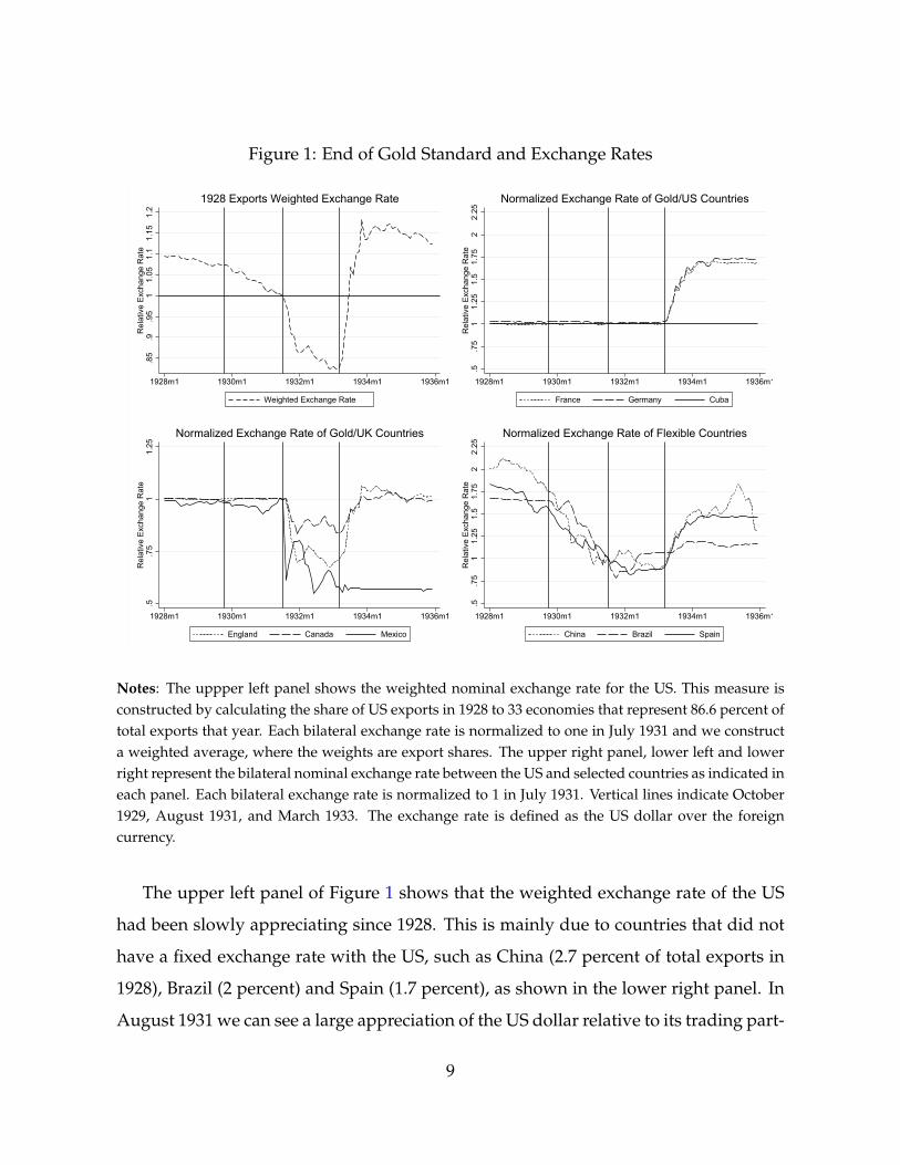
Figure 1: End of Gold Standard and Exchange Rates.8

5.9

.95

11.

051.

11.

151.

2R

elat

ive

Exch

ange

Rat

e

1928m1 1930m1 1932m1 1934m1 1936m1

Weighted Exchange Rate

1928 Exports Weighted Exchange Rate

.5.7

51

1.25

1.5

1.75

22.

25R

elat

ive

Exch

ange

Rat

e

1928m1 1930m1 1932m1 1934m1 1936m1

France Germany Cuba

Normalized Exchange Rate of Gold/US Countries

.5.7

51

1.25

Rel

ativ

e Ex

chan

ge R

ate

1928m1 1930m1 1932m1 1934m1 1936m1

England Canada Mexico

Normalized Exchange Rate of Gold/UK Countries

.5.7

51

1.25

1.5

1.75

22.

25R

elat

ive

Exch

ange

Rat

e

1928m1 1930m1 1932m1 1934m1 1936m1

China Brazil Spain

Normalized Exchange Rate of Flexible Countries

Notes: The uppper left panel shows the weighted nominal exchange rate for the US. This measure isconstructed by calculating the share of US exports in 1928 to 33 economies that represent 86.6 percent oftotal exports that year. Each bilateral exchange rate is normalized to one in July 1931 and we constructa weighted average, where the weights are export shares. The upper right panel, lower left and lowerright represent the bilateral nominal exchange rate between the US and selected countries as indicated ineach panel. Each bilateral exchange rate is normalized to 1 in July 1931. Vertical lines indicate October1929, August 1931, and March 1933. The exchange rate is defined as the US dollar over the foreigncurrency.

The upper left panel of Figure 1 shows that the weighted exchange rate of the US

had been slowly appreciating since 1928. This is mainly due to countries that did not

have a fixed exchange rate with the US, such as China (2.7 percent of total exports in

1928), Brazil (2 percent) and Spain (1.7 percent), as shown in the lower right panel. In

August 1931 we can see a large appreciation of the US dollar relative to its trading part-

9

ners. Mexico (2.6 percent) had a large depreciation of its currency that year as seen in

the lower left panel. Then, the most important trade partners of the US -Canada (17.1

percent of total exports in 1928), the UK (16.6 percent) and the countries tied to the

British pound- also depreciated their currencies. Other countries remained tied to the

gold, such as Germany (9.1 percent), France (4.7 percent), and Cuba (2.5 percent), so the

exchange rate with these countries was not affected in 1931, as seen in the upper right

panel. Then, when the US abandoned the gold standard, the US dollar experienced a

large depreciation. This was produced by a depreciation relative to the countries that

were not tied to gold, such as Canada and the UK, but also relative to the countries that

remained on the gold standard, such as France and Germany. Some few countries,such

as Cuba, remained tied to the US dollar.

Figure 2 shows that following these main events, measures of trade also reacted. Ex-

ports and quantities of exports decreased sharply during the Great Depression. Panels

1, 2 and 4, show that after the depreciation, exports experienced an increase as mea-

sured by value and volume. This trend coincided with the evolution of industrial pro-

duction, which also strongly increased starting in April 1933, as shown in panel 3 of

Figure 2.

These figures also show that the Great Depression was characterized by a large

drop in exports. The US was not able to gain competitiveness using its currency. This

situation was exacerbated when the UK and other economies tied to the British pound

depreciated their currencies in 1931. Before October 1929, exports were slowly growing

according to many measures, as well as economic activity. The gold standard worked

in a cooperative way until 1928 (Eichengreen (1996)), but as October 1929 approached,

that cooperation ended, producing a tightening of the money supply that increased

the effects of the great crash.9 During the years of the depression, real exports dropped

almost 70 percent while industrial production dropped by a similar magnitude.

9Bernanke (1995) argues that the largest factor behind the monetary contraction in the US was theinstability of the banking sector, while the collapse of the gold standard dominated outside the US.

10

Figure 2: End of Gold Standard and Trade10

020

030

040

050

0M

illion

s of

Dol

lars

in J

anua

ry 1

928

1928m1 1930m1 1932m1 1934m1 1936m1Date

Total Exports Total ImportsVertical lines are start of Great Depression and end of Gold Standard

Millions of DollarsTotal Exports and Imports

010

020

030

040

0M

illion

s of

Dol

lars

in J

anua

ry 1

928

1928m1 1930m1 1932m1 1934m1 1936m1Date

Manufacturing Exports Manufacturing ImportsVertical lines are start of Great Depression and end of Gold Standard

Millions of DollarsManufacturing Exports and Imports

4060

8010

012

0In

dex

(192

9m1=

100)

1928m1 1930m1 1932m1 1934m1 1936m1

Index of Industrial Production

1000

1500

2000

2500

3000

Thou

sand

s of

Lon

g To

ns

1928m1 1930m1 1932m1 1934m1 1936m1Date

U.S. Panama Canal Traffic, Cargo

Notes: The upper left panel (panel 1) is the seasonally adjusted total exports in millions of dollarsnormalized by the CPI (base January 2008). The data come from the NBER Macrohistory Database.The upper right panel (2) is the seasonally adjusted total exports in manufacturing in millions of dollarnormalized by the CPI (base January 2008). The data come from the NBER Macrohistory Database. Thelower left panel (3) shows monthly industrial production, normalized to January 1929 (100). The datacome from the Fed’s G.17 Industrial Production and Capacity Utilization. The lower right panel (4) isthe seasonally adjusted long tons of US cargo in the Panama Canal from the Panama Canal Record,available in the NBER Macrohistory Database. Each bilateral exchange rate is normalized to 1 in July1931. Vertical lines indicate October 1929, August 1931, and March 1933.

Depreciation lowers the price of American goods in terms of foreign currency, en-

hancing the competitiveness of exports. By March 1933, US exports reached their low-

est value since 1929. The manufacturing sector (66 percent of total exports in Septem-

ber 1929) was particularly hard hit. In March 1933, manufacturing exports in real terms

were 73 percent lower than in September 1929. Exports of crude materials (32.5 percent

11

of exports in September 1929) decreased 50 percent. By March 1934, manufacturing ex-

ports were 85 percent higher, while crude materials were 50 percent higher than one

year before. After that low point in March 1933, the value of exports grew by 75.21

percent over the next six months. This effect was not only caused for by rising prices.

By April 1934, the weight of US cargo in the Panama Canal was 53.3 percent higher

than in April 1933.

Relevant economic stakeholders at the time suggested that the volume of trade

could have been even much greater after the United States went off the gold standard.

The expansion of exports was hindered by the instability of the dollar. With the dollar

falling in value, it was convenient for foreign importers to delay purchases of Ameri-

can goods in anticipation of further depreciation. Patch (1934), quoting a speech made

in December 1933 by the head of the Foreign Credit Interchange Bureau of the National

Association of Credit Men, William S. Swingle, reveals the thinking of the time:

An imposing backlog of orders is piling up abroad while customers for American

products wait for the dollar to settle to a permanent level. They refuse to make ad-

vance commitments for fear competitors will be able to buy similar goods at a more fa-

vorable price later. A desire to profit by exchange is also having an effect upon collec-

tions in many foreign markets. Payments for shipments are being delayed in the hope

that the dollar will be lower when the final settlement for goods purchased is made.

According to him, foreign purchasers avoided making long-term commitments in

the hope of receiving more American goods for the same amount of money. Patch

(1934), now quoting the secretary of the Export Managers Club of New York, said:

“Foreigners are buying more goods, but their purchases are made up of small orders

placed at frequent intervals and represent no long-time commitments.”

Depreciation also increases the price of imports of the depreciated currency, which

would discourage the demand for foreign goods. However, after the United States

abandoned the gold standard in the spring of 1933, the value of imports (seasonally

adjusted) grew without interruption until August 1933, accumulating a growth of 84.6

12

percent as shown in Figure 2. The initial increase in imports is consistent with the

empirical evidence provided in Blaum (2019), who shows that large devaluations are

characterized by an increase in the aggregate share of imported inputs and by the re-

allocation of resources toward import-intensive firms, because large exporters are also

large importers (Amiti, Itskhoki, and Konings (2014), Bernard et al. (2007), and Al-

bornoz and Garcıa-Lembergman (2020)).10 The effect on net exports is ambiguous.11

This narrative and the quantitative evidence show that the external sector expanded

starting in April 1933.

The opposite mechanism occurred when other countries abandoned the gold stan-

dard. When the UK left the gold standard in September 1931, newspapers at the time

warned about the consequences for the US export sector. The New York Times, for ex-

ample, highlighted the potential gains for the UK, expecting an increase in England’s

exports while increasing American imports. The Times considered that the US would

experience “a temporary reduction in the standard of living.” The article was opti-

mistic about an increase in the UK’s demand for US raw materials, which can explain

why crude material exports did not decline as much as manufacturing exports during

the Great Depression. This optimism did not last long: On October 4, the same news-

paper documented that American cotton exports were stagnant. The paper attributed

this situation to the “decline in sterling values,” describing a “steady decline in prices.”

The article highlighted that it did not know when the price decline was going to stop.

We turn now to estimating the exchange rate mechanism empirically. In the next

section, we evaluate changes in competitiveness due to changes in the exchange rate

during the Great Depression. With this we can account for changes in the terms of trade

10Patch (1934) argues that the initial growth in imports was due to the sharp increase in industrialactivity and the need for replenishing stocks of raw materials. With the dollar falling in value, itwas convenient for importers to accumulate large stocks of foreign products in anticipation of furtherdepreciation of the dollar. According to this author, the loss of purchasing power of the US dollarbecame an obstacle for importers by July 1933, as reflected in the decline of the year-over-year growthrate of imports, while the export growth rate increased progressively after August 1933.

11The increase in net exports is related to the elasticity of substitution between the local and foreignvariety. We show and discuss this point in Appendix A.2.

13

to see if we should expect benefits for the external sector. Then, we measure the effect

on economic activity, comparing the economic performance of more export-oriented

cities relative to less export oriented cities.

3 Competitiveness Effect of Changes in Exchange Rate

We start by studying whether changes in exchange rates had an effect on prices.

The amount of pass-through is relevant for understanding the gain in competitiveness

for local producers. For example, if the US dollar depreciates by 1 percent, and at the

same time the prices of American products in the UK decrease by 1 percent, US pro-

ducers will receive the same revenue from any foreign sales. Pass-through of less than

1 percent will imply some gains in competitiveness for the US producer, as she will

receive more local currency for the same product.

In order to have incomplete pass-through in economics models, many works, such

as Atkeson and Burstein (2008), have focused on variable markups. Incomplete pass-

through can also be achieved in a New Keynesian model with sticky prices and some

level of substitution between varieties as in Monacelli (2005).12 In Appendix A.2 we

show that after a negative local shock, the external sector of the domestic country loses

competitiveness through an increase in the price of the tradable good produced do-

mestically relative to the price of the same good produced abroad. On the other hand,

under the flexible regime, the exchange rate buffers the loss of competitiveness, mit-

igating the negative impact of the shock. Consequently, under a fixed exchange rate,

the recession is deeper and longer lasting.

For this reason we start estimating exchange rate pass-thought, in order to evaluate

the extent of the gains in competitiveness. For this, we gather prices at the individual

goods level for the US, the UK, France and Germany. We do not have data for all of the

goods and all of these countries, but we do have data for all of the products at least in

12The market conditions to achieve that results were proposed in Dornbusch (1987)

14

the US.13 We use monthly data from 1928 to 1934 for most products .14 Then, we run

the following regression to see the effect of the exchange rate on prices:

∆Pricesc,j,t = β∆Exchange Ratec,t + γj,c + θj,t + εc,j,t, (1)

where Pricesc,j,t is the log of the price of the good j in country c at time t. Exchange Ratec,t

is the log bilateral exchange rate (US/c) with respect to country c at time t. We also

add a country-product fixed effect (γj,c) to control for the unit of the good, so we do

not have to worry if the price of the product is in pounds or kilograms, for example,

and a product-time fixed effect (θj,t) that controls for any general effect on prices and

also for any product-specific shock or seasonality. Standard errors are clustered at the

product-country level and at the time level.

In addition to this regression, we can see whether more tradable products have a

higher or lower pass-through. Every good has some tradable and nontradable compo-

nent, so we expect that β should be significant for all of the goods, but we expect that

the effect should be more pronounced for goods that have a higher tradable compo-

nent.15 Table 1 shows the results for the regression just mentioned.

13The products are bread (France and US), butter (UK and US), cattle (UK and US), copper (Germanyand US), cotton yarn (Germany and US), eggs (UK and US), hides (Germany and US), hogs (Germany,UK and US), milk (UK and US), oats (UK and US), pig iron (France, Germany, UK and US), potatoes(UK and US), poultry (UK and US) and wheat (France, Germany, UK and US).

14Data for pig iron not available for the UK in 1934, and data for wheat are available until November1934 for the UK and June 1934 for France

15We classify as tradable goods copper, cotton yarn, hides, oats, pig iron, potatoes and wheat

15

Table 1: Effect of Exchange Rate Changes on Prices(1) (2) (3) (4)

Exchange Rate (log changes) -0.500*** -0.522*** -0.507*** -0.232**(0.104) (0.119) (0.127) (0.105)

Exchange Rate*Tradable 0.044 -0.543**(0.116) (0.236)

Country-Product FE Yes Yes Yes YesTime FE Yes Yes - -Product-Time FE No No Yes YesObservations 2,719 2,719 2,719 2,719R-squared 0.071 0.071 0.590 0.592

Notes: The table shows the results of specification 1. The dependent variable is the change in log ofprices. The exchange rate is the change in logs of the exchange rate, measured as US dollars over oneunit of local currency (1 for the US). Tradable is a dummy equal to 1 for tradable goods. Clusters are atthe product-country level and at the time level. *** p<0.01, ** p<0.05, * p<0.1

We can see that the pass-through is not complete, which indicates a gain in com-

petitiveness. For example, after a 1 percent depreciation of the British pound, prices in

the UK are around 0.5 percent more expensive in pounds, meaning that those prices,

when converted to US dollars, are 0.5 percent cheaper for American consumers. This

effect is consistent over all the specifications. Consistent with Burstein, Eichenbaum,

and Rebelo (2005), we find higher pass-through for tradable goods as shown in column

(4). This means that even within the country, the effect shows that there are gains in

competitiveness in tradable goods. The average coefficient is in line with those found

in Goldberg and Knetter (1997) and Burstein and Gopinath (2014). For tradable goods

the coefficient is close to 0.8. This is a high pass-through, but close to and relatively

smaller than the one found by Gopinath, Itskhoki, and Rigobon (2010) for non dollar

invoiced goods and Auer, Burstein, and Lein (2021) for euro invoiced goods.

In addition to this result, we explore what happened during two important events

during the Great Depression. The first event occured in September 1931, when the UK

left the gold standard, producing an appreciation of the US dollar of more than 25 per-

cent relative to the British pound between September and December 1931, as shown in

16

Figure 1. This shock is relatively exogenous from the US point of view. There is no ev-

idence of changes in price expectations during that time (Binder (2016)). So, it is likely

that the policy conducted in the UK was not related to prices in the US. This considera-

tion will be more important when we discuss the results in terms of economic activity.

The second event occurred in April 1933, when the US left the gold standard. In

this exercise, we only use product prices between two countries and their bilateral ex-

change rate. We evaluate the effect of these events through the time series, exploring

the cross-sectional differences in prices in each period of time. We perform this exercise

between the US and the UK. For comparison, we also perform this exercise between

the US and Germany. The bilateral exchange rate between the US and Germany did

not change in 1931, so we should not see an effect that year. In 1933, the US dollar

also depreciated relative to the German mark, so we expect to see an effect around that

event of US prices relative to both British and German prices. We run the following

regression:

Pricesc,j,t = βt ×USc × γt + γj,c + εc,j,t, (2)

where USc is a dummy equal to 1 if the country is the US and γt is a time dummy. The

rest of the variables are the same as in the previous equation. We explore the effect

for both events of 1931 and 1933 and show the results for all of the time series to test

pre-trends and how persistent these effects are. Figure 3 shows the results.

17

Figure 3: Exchange Rate and Price Reaction after Gold Standard

.6.8

11.

2Ex

chan

ge R

ate

(US/

UK,

Aug

ust 1

931=

1)

-.4-.2

0.2

Log

Pric

es in

Loc

al C

urre

ncy

1931m1 1931m7 1932m1 1932m7 1933m1

Coefficient 95% Exchange Rate

1931US Prices Relative to UK Prices

.81

1.2

1.4

1.6

Exch

ange

Rat

e (U

S/U

K, M

arch

193

3=1)

-.20

.2.4

.6Lo

g Pr

ices

in L

ocal

Cur

renc

y

1932m1 1932m7 1933m1 1933m7 1934m1 1934m7

Coefficient 95% Exchange Rate

1933US Prices Relative to UK Prices

.6.8

11.

2Ex

chan

ge R

ate

(US/

Ger

man

, Aug

ust 1

931=

1)

-.4-.2

0.2

Log

Pric

es in

Loc

al C

urre

ncy

1931m1 1931m7 1932m1 1932m7 1933m1

Coefficient 95% Exchange Rate

1931US Prices Relative to German Prices

.81

1.2

1.4

1.6

Exch

ange

Rat

e (U

S/G

erm

an),

Mar

ch 1

933=

1

-.20

.2.4

.6Lo

g Pr

ices

in L

ocal

Cur

renc

y

1932m1 1932m7 1933m1 1933m7 1934m1 1934m7

Coefficient 95% Exchange Rate

1933US Prices Relative to German Prices

Notes: The figure represents results from regression (2). The left panels represent results when the UKabandoned the gold standard in September 1931 and the right panels represent the event when the USleft the gold standard in April 1933. The top two panels represents results of equation (2) for the US andthe UK and the bottom two panels represent results of equation (2) for the US and Germany. The solidline represents the coefficient of the regression (βt) for each period of time, which shows the reaction ofUS prices relative to the other economy. The light-dashed line represents confidence intervals at the 95percent level. Standard errors have two-way clusters at the product-country level and at the time level.The dark-dashed line represents the bilateral exchange rate.

The figure shows a similar pattern compared with the general regression in Table 1.

After the UK left the gold standard, US prices declined relative to UK prices at a lower

rate than the appreation of the US dollar, implying a reduction in the competitiveness

of the US relative to the UK. The opposite effect occurred in 1933. After the US went

off the gold standard, US prices increased relative to UK prices at a lower rate than the

depreciation of the US dollar, implying a gain in the competitiveness of the US relative

18

to the UK. These changes are large. By August 1932, prices in the US were 16 percent

lower than in the UK. This effect is the result of a 28 percent appreciation of the US

dollar. A similar effect was produced over the same period of time (one year), but in

1933. US prices in March 1934 were 35 percent higher than in March 1933, after a 48

percent depreciation of the US dollar.

Relative prices between the US and Germany were less affected by the UK’s depar-

ture from the gold standard. The results show only a mild reduction in bilateral prices

around this event.16 This shows that the change in prices did not come from some spe-

cific change in the US relative to all the other countries. In 1933, the change in relative

prices between the US and Germany is similar to the change in relative prices between

the US and UK.17

The results found in this section are consistent with an incomplete pass-through.

This incomplete pass-through is present around the main events that we analyze in

this paper as well. From the price results, the implication is that exporters gained com-

petitiveness in 1933, but the ones exposed to the UK in 1931 lost competitiveness. In

the next section, using detailed cross-sectional variation in the US, we evaluate whether

changes in competitiveness had an impact on the level of economic activity

4 Local Effect of Exchange Rate Changes on Economic

Activity

We evaluate the effect on local economic activity. We use data on bank debits for

more than 200 cities available on a weekly basis. As shown in Pedemonte (2020), this

measure strongly correlates with measures of spending on durable goods. This mea-

16According to Gopinath et al. (2020) pass-through of import prices should be driven by changesin the dominant currency. Eichengreen and Flandreau (2009) using data from Nurkse (1944) show thatup to the 1930s the pound was still the dominant currency, but the US was also an important sourceof currency reserves. The British pound has been a more dominant currency for the United States thanfor Germany can explain why prices in the US might have declined slightly relative to the prices inGermany following the depreciation of the British pound. In any case, these relative changes are small.

17Note that this result is consistent with the British pound as a dominant currency.

19

sure highly predicts measures of economic activity, such as car spending, department

store sales, industrial production and business activity, at the state, federal reserve dis-

trict and national level on a monthly basis (see Appendix A.1, Tables A.1 and A.2). We

aggregate these data to a monthly frequency and seasonally adjust the series.18 This

is relevant, since we are going to control for the economic characteristics of the cities,

which can have important seasonal fluctuations, in particular in sectors such as agri-

culture.

We construct a measure of the exposure to changes in the exchange rate at the city

level. In order to do this, we combine country sector-specific exports for the US in

1928, the bilateral exchange rate from 1928 to 1935, and city-level sectoral employ-

ment shares from the census of 1930 (Ruggles et al. (2021)). With this information, we

construct a time-varying indicator that combines the specific exposure of a city to a

country, through its economic specialization and get the variation over time through

fluctuations in the bilateral exchange rate. Specifically, we construct the following mea-

sure of exposure:

Exposure Tradec,t = ∑s

Sh Ws,c,1930 ∑d

Sh Exs,d,1928 × RERd,t, (3)

where c indexes cities and t indexes dates. Sh Ws,c,1930 represents the share of workers

in sector s in city c according to the census of 1930. Sh Exs,d,1928 is the sector’s export

share going to destination d and RERd,t is the relative bilateral nominal exchange rate

of the US relative to destination d normalized to 1 in July 1931.

In order to combine the census industrial employment data with the sectoral trade

information, we make a correspondence between both sources of information as de-

scribed in Table A.3 in Appendix A.1. We have 45 sectors that represent US merchan-

dise exports to 33 destinations. This information gives enough variation in terms of the

18We take logs and run a regression with city-month fixed effects. Then, we obtain the residual ofthe regression.

20

exposure to trade to different destinations. While Canada and the UK were the main

trading partners of the US, Japan, for example, dominated in forestry and fertilizers.

Mexico dominated in explosives and firearms, the Netherlands in precious stones and

Germany in cotton. Also, while iron ore went mainly to Canada and the UK, only 12

percent of explosives and firearms went there in our sample. This variation gives us

exposure to different exchange rate regimes and shocks.

Exposure Tradec,t incorporates the variation at the city level and across time. Con-

sidering the cross-sectional variation, the average value for each city shows how ex-

posed to trade a city is relative to other cities. But it also incorporates the variation that

is relevant given the exchange rate dynamics present in the Great Depression. For ex-

ample, China had a flexible exchange rate with the US. This means that cities exposed

to a sector where China is an important destination were losing competitiveness since

the beginning of the Great Depression, but if those cities where not exposed to sectors

were the UK or pound-tied countries were important, the appreciation of 1931 should

have not been so relevant for those cities. At the same time, cities more exposed to

France or Germany should benefit relatively more from the depreciation of 1933. This

is also a direct measure of exposure, since it does not consider the exposure of the

destination to other countries, through the same sector.

In order to illustrate the characteristics of this measure, we take two cities as exam-

ples: Pueblo, CO, and New Bedford, MA. Pueblo is an inland city, with geographical

conditions less favorable to international trade. Surprisingly, this city had the median

allocation of labor to exporting sectors according to our sample: 35.3 percent of its

working population. This city had the main plant of the Colorado Fuel and Iron Com-

pany, an important steel conglomerate. Eighteen percent of the labor force of Pueblo

worked in the steel manufacturing sector. The main destination of this sector’s product

was Canada, with 44 percent of the total exports in our sample and then Japan, with 18

percent. On the other hand, New Bedford was a city open to international trade. Lo-

cated in the coast of Massachusetts, the city had direct access to the Atlantic. This could

21

explain why 55 percent of the city’s labor force worked in the exporting sector. They

specialized in textiles, another important exporting sector of the US. Forty-two per-

cent of its working population was employed in the cotton sector, distributed among

several cotton mills in the city. The main destination of the semi-manufactured cotton

products was Germany (25 percent of all the exports in our sample ) and the UK (24

percent). These characteristics of the employment of the cities exposed them to differ-

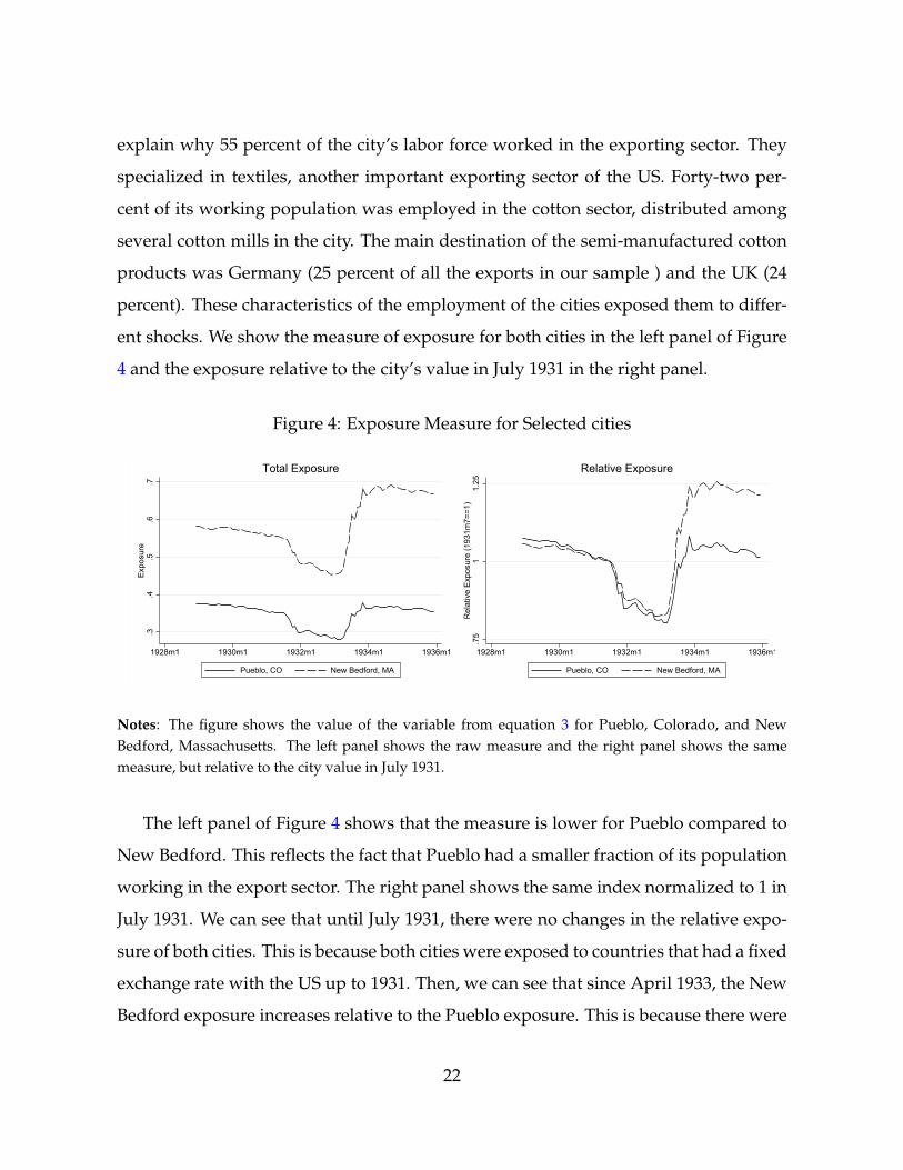
ent shocks. We show the measure of exposure for both cities in the left panel of Figure

4 and the exposure relative to the city’s value in July 1931 in the right panel.

Figure 4: Exposure Measure for Selected cities

.3.4

.5.6

.7Ex

posu

re

1928m1 1930m1 1932m1 1934m1 1936m1

Pueblo, CO New Bedford, MA

Total Exposure.7

51

1.25

Rel

ativ

e Ex

posu

re (1

931m

7==1

)

1928m1 1930m1 1932m1 1934m1 1936m1

Pueblo, CO New Bedford, MA

Relative Exposure

Notes: The figure shows the value of the variable from equation 3 for Pueblo, Colorado, and NewBedford, Massachusetts. The left panel shows the raw measure and the right panel shows the samemeasure, but relative to the city value in July 1931.

The left panel of Figure 4 shows that the measure is lower for Pueblo compared to

New Bedford. This reflects the fact that Pueblo had a smaller fraction of its population

working in the export sector. The right panel shows the same index normalized to 1 in

July 1931. We can see that until July 1931, there were no changes in the relative expo-

sure of both cities. This is because both cities were exposed to countries that had a fixed

exchange rate with the US up to 1931. Then, we can see that since April 1933, the New

Bedford exposure increases relative to the Pueblo exposure. This is because there were

22

no significant changes in the bilateral exchange rate with Japan, while the US dollar

depreciated sharply against the German mark. Overall, we can see that the measure

combines general exposure to trade, with time series variations reflecting exposure to

countries and their exchange rate movements.

We use this variable to evaluate the effect of trade on economic activity. Using

monthly data, we run the following regression:

Dc,t = γc + γt + β× Exposure Tradec,t + εc,t, (4)

where Dc,t is the log of bank debits in city c at time t. We do not have many controls

at the city-monthly level, so we include a city fixed effect in all specifications. We

do this to focus on the variation in debits within the city, independent of the size.

We include a time fixed effect to control for the common variation and focus on the

cross-sectional variation given by changes in the relative exchange rate by individual

countries. In some specifications, we include state-time fixed effects to control for any

common change at the state level or Fed-time fixed effects to control for any common

change at the Federal Reserve District level. Errors are clustered at the city level. Table

2 shows the results.

23

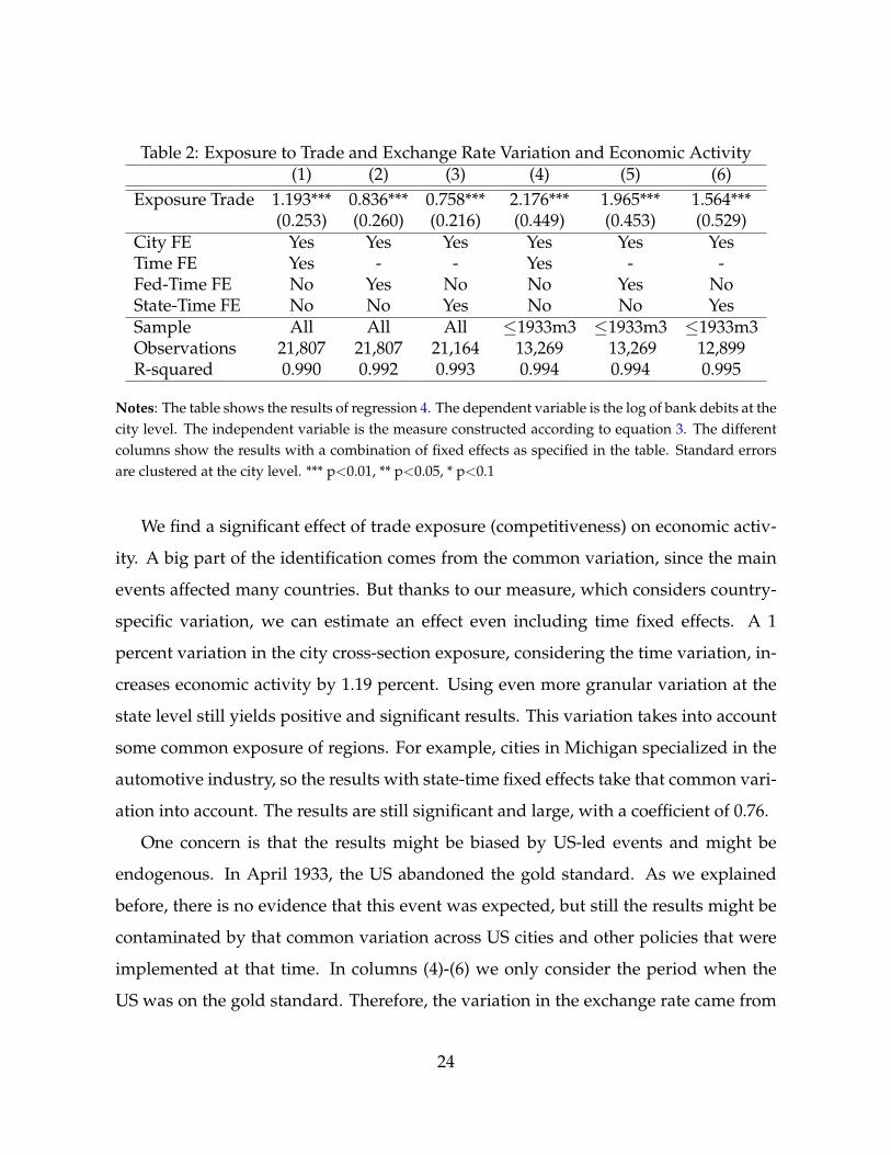
Table 2: Exposure to Trade and Exchange Rate Variation and Economic Activity(1) (2) (3) (4) (5) (6)

Exposure Trade 1.193*** 0.836*** 0.758*** 2.176*** 1.965*** 1.564***(0.253) (0.260) (0.216) (0.449) (0.453) (0.529)

City FE Yes Yes Yes Yes Yes YesTime FE Yes - - Yes - -Fed-Time FE No Yes No No Yes NoState-Time FE No No Yes No No YesSample All All All ≤1933m3 ≤1933m3 ≤1933m3Observations 21,807 21,807 21,164 13,269 13,269 12,899R-squared 0.990 0.992 0.993 0.994 0.994 0.995

Notes: The table shows the results of regression 4. The dependent variable is the log of bank debits at thecity level. The independent variable is the measure constructed according to equation 3. The differentcolumns show the results with a combination of fixed effects as specified in the table. Standard errorsare clustered at the city level. *** p<0.01, ** p<0.05, * p<0.1

We find a significant effect of trade exposure (competitiveness) on economic activ-

ity. A big part of the identification comes from the common variation, since the main

events affected many countries. But thanks to our measure, which considers country-

specific variation, we can estimate an effect even including time fixed effects. A 1

percent variation in the city cross-section exposure, considering the time variation, in-

creases economic activity by 1.19 percent. Using even more granular variation at the

state level still yields positive and significant results. This variation takes into account

some common exposure of regions. For example, cities in Michigan specialized in the

automotive industry, so the results with state-time fixed effects take that common vari-

ation into account. The results are still significant and large, with a coefficient of 0.76.

One concern is that the results might be biased by US-led events and might be

endogenous. In April 1933, the US abandoned the gold standard. As we explained

before, there is no evidence that this event was expected, but still the results might be

contaminated by that common variation across US cities and other policies that were

implemented at that time. In columns (4)-(6) we only consider the period when the

US was on the gold standard. Therefore, the variation in the exchange rate came from

24

foreign policy decisions. We can see that the coefficients are not only significant, but

even larger: including time fixed effects, a 1 percent variation in the city cross-section

exposure increases economic activity by 2.17 percent. These results are in line with

Obstfeld, Ostry, and Qureshi (2019), who show that under fixed regimes, global shocks

are magnified.

Next, we estimate the contribution of trade exposure to the depth of the Great De-

pression between 1931 and 1932 and to the recovery between 1933 and 1934. For sim-

plicity, we use a version of equation 4 with a unique time fixed effect. Then, we assess

the contribution of the average effect over the cities β × Exposure Tradec,t compared

with the time effect γt, around the two main events covered in this paper. In particu-

lar, we will show how much of the total change in economic activity after those events

can be attributed to the trade channel. This analysis abstracts from spillover effects and

only shows direct effects. In a sense, it would be a lower bound of the total contribution

of the trade channel.

As we showed before, when large changes in the exchange rate occurred, not every

city was exposed in the same way to trade. Actually, only 35 percent of the work-

ers in our sample were employed in trade sectors according to our classification, and

that percentage varies from cities with less than 5 percent, such as Washington DC, to

others with more than 70 percent, such as Elberton, GA. This variation interacts with

changes in the exchange rate, creating variation even when there are some common

movements. Because of this, the time fixed effect captures common movements, tak-

ing into consideration cities that were almost unexposed in our sample. In the next

subsection, we evaluate the event of 1931.

4.1 UK’s Exit and Trough of the Great Depression

We first analyze what happened to the external sector after the large appreciation of the

US dollar in 1931. This event was the consequence of policies implemented by other

countries to deal with their respective local crises. As discussed before, Mexico exited

25

in August 1931 and the UK in September 1931. In this sense, the event is exogenous

relative to our observation units, which are particular cities in the US.

Figure 5 plots the total average effect γt + β × Exposure Tradec,t versus the time

fixed effect γt. For both cases, it shows the changes over its own level in July 1931. As

the dependent variable is in logs, this approximates to percentage changes with respect

to the level of each effect in that period of time.

Figure 5: Effect of Exchange Rate Appreciation on Trade-Exposed Cities

-.6-.4

-.20

.2R

elat

ive

coef

ficie

nt

1931m1 1931m7 1932m1 1932m7 1933m1

Total Effect Time FE

Decomposition Around UK Exit

Notes: The figure plots the changes in the average time fixed effect γt and the average total effectγt + β× Exposure Tradec,t relative to July 1931. The result comes from regression 4 reported in Table 2

Figure 5 shows a large reaction of trade-exposed cities. After having similar trends,

cities more exposed to trade show a large decrease in economic activity after August

1931 relative to the rest of the sample, conditional on their individual exposure to

changes in the exchange rate. This effect is economically significant. As shown in

Figure 5, on average, the economy had reduced its economic activity by 16 percent by

the end of 1931 and around 40 percent of that effect was due to trade exposure. After

that, the economy continues to decline. By the end of 1932, the trade exposure effect

directly accounted for 16 percent of that effect.

This result shows that the effect of the trade channel was relevant compared with

26

the common trends in the economy at that time. This is a direct effect, meaning that

we do not estimate any other type of multiplier. The appreciation of the US dollar in

1931 was strong, but the depreciation of 1933 was much greater in magnitude. In the

next subsection, we evaluate the recovery starting in April 1933.

4.2 Recovery

In April 1933, the US left the gold standard and the US dollar depreciated relative to

other currencies, as shown in Figure 1. The abandonment of the gold standard was part

of the plan of the Democratic party according to Eggertsson (2008) and not expected

until March 1933 (Hsieh and Romer (2006)). But the change in policy was accompanied

by many other policy changes. Many factors can explain the recovery that the economy

experienced beginning in the spring of 1933. Some work has focused on expectation

channels, whereby higher inflation expectations induced by Roosevelt’s policies re-

duced the ex-ante real interest rate, stimulating investment and consumption through

traditional channels (Eggertsson (2008), Jalil and Rua (2016), Sumner (2015), and Tay-

lor and Neumann (2016)). Other work focuses on the role of public debt in the context

of higher inflation; see, for example, Jacobson, Leeper, and Preston (2019). Hausman,

Rhode, and Wieland (2019) argue that higher inflation coming from higher traded crop

prices redistributed income from lenders (nonfarm households and businesses) with a

relatively low marginal propensity to consume, to debtors (farmers) with a relatively

high marginal propensity to consume. Cole and Ohanian (2004) argue that the recov-

ery from the Great Depression was weak due to New Deal cartel-type policies.

In order to evaluate the contribution of the trade channel relative to that of other

policies, we perform the same exercise as in the previous subsection, but relative to

February 1933 to capture the contribution of the depreciation. The other policies im-

plemented at the time do not seem to have a special focus on the external sector, so

those considerations will be captured by common trends (time fixed effects) if they

affected trade cities in the same way as nontrade cities. Figure 6 shows the effect fol-

27

lowing the abandonment of the gold standard by the US.

Figure 6: Trade Exposure Effect and US Abandons the Gold Standard

-.10

.1.2

.3R

elat

ive

coef

ficie

nt

1933m1 1933m7 1934m1 1934m7 1935m1

Time FE Total Effect

Decomposition Around US Exit

Notes: the figure plots the changes of the average time fixed effect γt and the average total effect γt +

β× Exposure Tradec,t relative to February 1933. The result comes from regression 4 reported in Table 2

As Figure 6 shows, in this case the trade channel’s contribution is very important.

We observe that after April 1933, more exposed cities experienced a large increase in

their economic activity. After March 1933 there is a drop on average. That month was

characterized by a bank holiday, so there are fewer observations for our sample and

some cities show very small numbers that month. After that, there is an immediate

increase in economic activity in more exposed cities. This effect is persistent. More

exposed cities continued to have a higher level of economic activity. Overall, we can

see that the trade channel also played an important role in the recovery that occurred

after 1933.

The effect is large. We can see that the contribution of the trade channel is particu-

larly important in 1933. By the end of that year, all the effect in terms of the recovery

was due to the trade exposure, where cities on average increased their economic ac-

tivity around 10 percent relative to February, even if the common trend was negative.

Starting in 1934, the average time fixed effect is positive. By April 1934, the average

28

total effect was 20 percent relative to February 1933, and the trade channel contributed

more than 60 percent of the total effect. By the end of 1934 the contribution was still

over 50 percent. We can see that the trade channel was the main driver of the economic

recovery that started in 1933 and it continued to be relevant effect after that year.

These results were obtained with very granular data at the city level, but a good

part of the variation is common to the cities. In the next section, we construct a mea-

sure of the increase in economic activity an we interact it with time dummies, to not

rely on the effect of the exchange and see how income translated to spending. We use

these results as robustness.

5 Robustness Using Bartik

In this section, we use another measure of trade exposure as a robustness test, ex-

ploiting the growth rates of the export sectors between 1932 and 1933. This measure

will closely indicate the increase in income that cities received given their sectoral ex-

posure to trade. We rely on the main events analyzed before -the UK exit in 1931 and

the US exit in 1933- to evaluate the effect of changes in the exchange rate on the eco-

nomic activity of export-oriented cities. For this empirical exercise, instead of using

the changes in the exchange rate, we rely only on time fixed effects interacted with the

measure of exposure to an increase in exports to see whether more exposed cities had

a relatively stronger economic recovery compared with less exposed cities.

In particular, we build a constant city level measure of exposure to trade. As in

the previous section, we get industrial employment at the county and industry level in

1930. Then, we obtain data on the sectoral exports of the US between April 1932 and

March 1933 and compared it with the data between April 1933 and March 1934. With

that information, we construct the following measure of exposure a la Autor, Dorn,

and Hanson (2013):

29

Trade Exposurec,33−32 = ∑s

Lc,s,1930

Lc,1930× Exportss,1934m3 − Exportss,1933m3

Exportss,1933m3, (5)

where Lc,s,1930 is the employment in 1930 in county c and sector s, Lc,1930 is total em-

ployment in county c, and Exportss,y is total exports in sector s over the last 12 months

of y.19 The data on economic activity are at the city level, but we use employment

at the level of the county where the city is located.20 This measure of exposure com-

bines the sectoral employment composition of the county where the city is located with

goods-level information on exports in terms of the US products that were more in de-

mand abroad. Table A.4 shows the composition of merchandise exports between April

1932 and March 1933 and the annual growth rate of the value of exports from April

1933 to March 1934, compared with April 1932-March 1933 by type of commodities.

The main exports are unmanufactured cotton (21.4 percent), petroleum and products

(13.9 percent), automobiles and other vehicles (6.1 percent), tobacco and manufactures

(4.6 percent) and fruits and nuts (4.9 percent).21 The product categories that experi-

enced the highest growth in the value of their exports by March 1934 were iron and

steel semi-manufactures (157.8 percent), meat products (62.7 percent), nonferrous met-

als (55.5 percent), automobiles (50.0 percent), other nonmetallic mineral products (49.9

percent), wood semi-manufactures (46.7 percent), unmanufactured cotton (46.1 per-

cent) and tobacco (36.8 percent). We can see that the sectors that grew the most were

related to the metal manufacturing industry and some agricultural sectors, such as

cotton, which is concentrated in certain areas of the country.

With this measure we will show which cities grew more after the shock in 1933,

19Table A.3 in Appendix A.1 contains the correspondence between export sectors and industrialsectors.

20Some cities were independent, in which case we only use city level employment.21It is estimated that in 1934 the production of goods for export provided a direct living for about 2

million people; approximately 1 million were cotton farmers and another half a million were engagedin other agricultural activities. Additionally, several million benefited indirectly by supplying goodsand services to the export sector (Patch (1935)).

30

relative to the lowest level of exports in 1932. This could be seen as a direct effect. A

city that exported more will have an increase in economic activity if exports rise. But,

in our estimations, we will compare the growth of the more exposed cities relative to

less export-dependent cities, so we are estimating the additional direct effect on the

exposed cities. In the case where other policies were more important (for example,

those that benefited the financial sector), this coefficient should not be positive or even

negative. Because of that, this marginal effect will measure whether the more exposed

cities benefited more, relative to the any other common effect or specific effect in other

industries.

As in the previous section, we estimate the effect of the appreciation of 1931 on

economic activity in trade-exposed cities. Here, we will not use the changes in the ex-

change rate; instead, we will use the across-time variation as a source of identification

because that the largest appreciation occurred at a specific period. We can compare the

pre-trends with the performance of the more exposed cities following the appreciation.

This event occurred outside the US so it is unlikely that a more exposed city could have

influenced that event. We run the following specification:

Dc,t = αc + γs(c),t +T

∑τ=0

βτ × Trade Exposurec,33−32 × 1τ + εi,t, (6)

where Dc,t is the seasonally adjusted log debits, Trade Exposurec,33−32 is the trade ex-

posure measure shown in equation 5, γs(c),t is a state-time fixed effect and αc is a city

fixed effect. 1τ is an indicator variable that is one for year τ. The regression includes

time-specific effects, meaning that βτ will capture differential outcomes across more

and less exposed cities. This empirical design implies that the coefficient βτ represents

the time fixed effect of average exposed cities relative to a baseline that considers the

average effect of the rest of our sample. In 1931, the economic activity of the whole

country was decreasing. γs(c),t will capture that effect even at the state level. The left

31

panel of Figure 7 shows how more exposed cities behaved after the appreciation of

the US dollar, given the shock of several countries exiting the gold standard. In the

right panel, we show the contribution of this effect relative to the average effect over

the cities at each period of time. We compute the average time effect (γs(c)t), and the

average exposed effect (γs(c)t + βt × Trade Exposurec,33−32).

Figure 7: Effect of Exchange Rate Appreciation on Trade-Exposed Cities

-1-.5

0.5

Log

Deb

its

1931m1 1931m7 1932m1 1932m7

Coefficient 95%

Average Exposed Effect

-.4-.2

0.2

Log

Deb

its

1931m1 1931m7 1932m1 1932m7

Average Time Effect Average Total Effect

Total and Time Effect

Notes: The right panel shows the results from the regression of the specification in equation 6. Thesolid line represents the coefficient βt. The coefficient is relative to July 1931 (equal to 0). The dashedlines represent confidence intervals at the 95 percent level. Standard errors are two-way clustered atthe city and time level. The right panel plots the average time effect γs(c)t and the average total effectγs(c)t + βt × Trade Exposurec,33−32.

After having similar trends, cities more exposed to trade show a large decrease in

economic activity after August 1931 relative to the rest of the sample. This effect is

economically relevant. As shown in the left panel of Figure 7, the average exposure

compared with the common trend of cities (time fixed effects) represents around a

third of the effect by 1932.

These effects are large. The average measure of exposure is 0.136 and the standard

deviation is 0.091. This means that in August 1932, an average trade-exposed city de-

creased its economic activity by 10 percent, relative to a less exposed city even in the

same state. We can see in the right panel of Figure 7 that the contribution of this effect

32

is economically significant. These results are similar to those found in the previous

section.

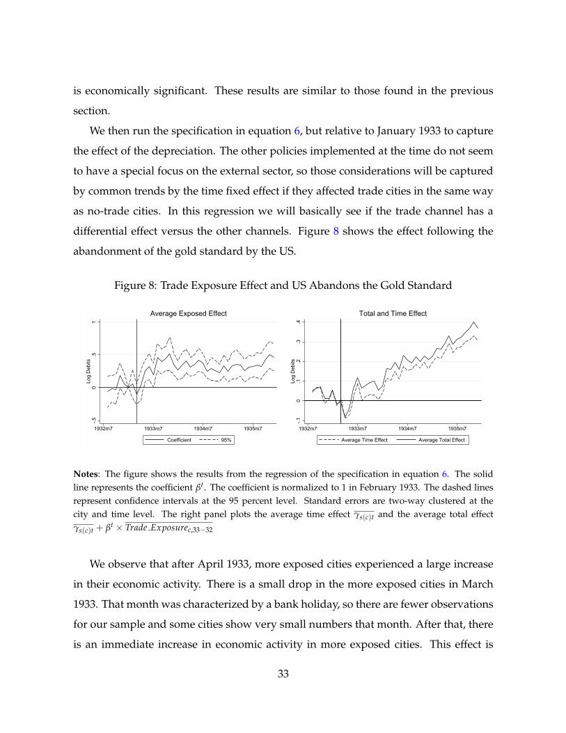
We then run the specification in equation 6, but relative to January 1933 to capture

the effect of the depreciation. The other policies implemented at the time do not seem

to have a special focus on the external sector, so those considerations will be captured

by common trends by the time fixed effect if they affected trade cities in the same way

as no-trade cities. In this regression we will basically see if the trade channel has a

differential effect versus the other channels. Figure 8 shows the effect following the

abandonment of the gold standard by the US.

Figure 8: Trade Exposure Effect and US Abandons the Gold Standard

-.50

.51

Log

Deb

its

1932m7 1933m7 1934m7 1935m7

Coefficient 95%

Average Exposed Effect

-.10

.1.2

.3.4

Log

Deb

its

1932m7 1933m7 1934m7 1935m7

Average Time Effect Average Total Effect

Total and Time Effect

Notes: The figure shows the results from the regression of the specification in equation 6. The solidline represents the coefficient βt. The coefficient is normalized to 1 in February 1933. The dashed linesrepresent confidence intervals at the 95 percent level. Standard errors are two-way clustered at thecity and time level. The right panel plots the average time effect γs(c)t and the average total effectγs(c)t + βt × Trade Exposurec,33−32

We observe that after April 1933, more exposed cities experienced a large increase

in their economic activity. There is a small drop in the more exposed cities in March

1933. That month was characterized by a bank holiday, so there are fewer observations

for our sample and some cities show very small numbers that month. After that, there

is an immediate increase in economic activity in more exposed cities. This effect is

33

persistent. More exposed cities continued to have a higher level of economic activity.

Overall, we can see that the trade channel also played an important role in the recovery

that occurred of 1933.

The coefficient is close to 0.5 by the end of 1933, which represents on average 7

percent more economic activity compared to the average growth. As explained before,

many other policies were implemented at that time. Many of those are captured by

the state-time fixed effect. The results show that more exposed cities grew relative to

the rest of the sample. This indicates that the trade channel accounts for a significant

differential effect, in a period when the whole country was growing. Considering this

estimation, the contribution of the trade channel is similar to the numbers obtained in

the previous section.

These results show that cities that increased their exports-related income because of

their trade-exposure and increased their exports due to the exit of the US from the gold

standard also significantly increased their spending relative to the other cities. Also,

these results show that those same cities were particularly affected when the UK left

the gold standard.

With this specification we can map the whole Great Depression and see how trade-

exposed cities behaved. Also, we do not rely on data on the exchange rate, which

experienced changes over time. In the next figure, we plot the coefficient of the re-

gression 6, between 1929 and 1936, representing the whole Great Depression and the

recovery before the crisis of 1937. We normalize the coefficient to 0 in June 1929.

34

Figure 9: Trade Exposure Effect and the Great Depression

-1.5

-1-.5

0.5

Log

Deb

its

1928m1 1930m1 1932m1 1934m1 1936m1 1938m1

Coefficient 95%

Notes: The figure shows the results from the regression of the specification in equation 6. The solid linerepresents the coefficient βt. The coefficient is normalized to 0 in June 1929. The dashed lines representconfidence intervals at the 95 percent level. Standard errors are two-way clustered at the city and timelevel. Vertical lines represent October 1929, August 1931, and March 1933

We can see an interesting pattern that coincides with some main events during the

Great Depression. There is a stable relationship in the level of economic activity be-

tween exposed and nonexposed cities until June 1930, when the Smoot-Hawley Tar-

iff Act was signed, and exposed cities lost ground relative to nonexposed cities. The

Smoot-Hawley Tariff Act produced a trade war in which countries retaliated by boy-

cotting US products, which can explain why export-oriented cities were affected (see

Mitchener, Wandschneider, and O’Rourke (2021)). Then, when the UK and its major

trading partners went off the gold standard, exposed cities were hit hard once again.

There is an incomplete recovery when the US left the gold standard in April 1933 and

exposed cities began to improve relative to nonexposed cities during the second half of

1935, when President Roosevelt signed trade agreements with the main trading part-

ners of the US (e.g. with Canada in November 1935). Exposed cities converged to the

level of less exposed cities at the state level only by the end of 1936.

These results show the importance of the trade channel during the Great Depres-

35

sion. US exporting cities were significantly affected relative to less dependent cities in

the US, and their recovery depended on the devaluation of the exchange rate and the

creation of trade agreements.

6 Conclusion

This paper explores the effect that the gold standard as a fixed exchange rate sys-

tem had on the US economy during the Great Depression. Using novel micro data, we

show that the terms of trade adjusted after the large currency changes that occurred

when countries abandoned the gold standard. We show that the US was affected by the

exit of the UK. The average trade-exposed city led the economic decline in economic

activity in 1931. We also find that the opposite happened when the US abandoned the

gold standard. This paper shows that the trade channel played an important role in

the depth of and the recovery from the Great Depression.

This channel adds to others that have been analyzed in the literature, but it has the

advantage that we tested it in a different context than the recovery of 1933, when many

other policies were implemented at the same time.

This paper shows that fixed exchange rate regimes contributed to economic crises

of the past and can have important implications today. Some type of fixed exchange

rate is still used by a large number of countries according to recent evidence (Ilzetzki,

Reinhart, and Rogoff (2019)). Our results show that those regimes could have detri-

mental effects for their external sectors in the case of negative shocks. Moreover, coun-

tries belonging to currency unions, such as those of the Eurozone, have experienced

different recovery paths since the Great Recession. In a world with high financial and

trade integration, limiting the ability of the exchange rate to adjust can have important

sectoral implications that could translate into deep economic recessions.

This paper also shows that relaxing those pegs could be beneficial for economic re-

covery. In this paper we show that exporting cities experienced an almost immediate

recovery compared with nonexporting cities when the dollar depreciated in 1933. As

36

Friedman (1953) pointed out, the exchange rate is a relatively flexible price that allows

the rest of the prices in the economy to adjust relative to those in other countries. The

results of this paper confirm that logic and highlight the importance of that mechanism

in buffering macroeconomic shocks.

37

References

Albornoz, Facundo and Ezequiel Garcıa-Lembergman. 2020. “Importing After

Exporting.” Unpublished Manuscript .

Amiti, Mary, Oleg Itskhoki, and Jozef Konings. 2014. “Importers, Exporters, and

Exchange Rate Disconnect.” American Economic Review 104 (7):1942–78. DOI

https://doi.org/10.1257/aer.104.7.1942.

Atkeson, Andrew and Ariel Burstein. 2008. “Pricing-to-Market, Trade Costs, and

International Relative Prices.” American Economic Review 98 (5):1998–2031. DOI

https://doi.org/10.1257/aer.98.5.1998.

Auer, Raphael, Ariel Burstein, and Sarah M. Lein. 2021. “Exchange Rates and Prices:

Evidence from the 2015 Swiss Franc Appreciation.” American Economic Review

111 (2):652–86. DOI https://doi.org/10.1257/aer.20181415.

Autor, David H., David Dorn, and Gordon H. Hanson. 2013. “The China Syndrome:

Local Labor Market Effects of Import Competition in the United States.” American

Economic Review 103 (6):2121–68. DOI https://doi.org/10.1257/aer.103.6.2121.

Bernanke, Ben S. 1995. “The Macroeconomics of the Great Depression: A Com-

parative Approach.” Journal of Money, Credit and Banking 27 (1):1–28. DOI

https://doi.org/10.2307/2077848.

Bernard, Andrew B., J. Bradford Jensen, Stephen J. Redding, and Peter K. Schott. 2007.

“Firms in International Trade.” Journal of Economic Perspectives 21 (3):105–130. DOI

https://doi.org/10.1257/jep.21.3.105.

Binder, Carola Conces. 2016. “Estimation of Historical Inflation Expectations.” Explo-

rations in Economic History 61:1–31. DOI https://doi.org/10.1016/j.eeh.2016.01.002.

Blaum, Joaquin. 2019. “Global Firms in Large Devaluations.” Unpublished Manuscript,

Brown University .

38

Bordo, Michael D. and Christopher M. Meissner. 2020. “Original Sin and the Great

Depression.” DOI https://doi.org/10.3386/w27067.

Burstein, Ariel, Martin Eichenbaum, and Sergio Rebelo. 2005. “Large Devaluations

and the Real Exchange Rate.” Journal of Political Economy 113 (4):742–784. DOI

https://doi.org/10.1086/431254.

Burstein, Ariel and Gita Gopinath. 2014. “International Prices and Exchange

Rates.” In Handbook of International Economics, vol. 4. Elsevier, 391–451. DOI

https://doi.org/10.1016/B978-0-444-54314-1.00007-0.

Campa, Jose Manuel. 1990. “Exchange Rates and Economic Recovery in the 1930s:

An Extension to Latin America.” Journal of Economic History 50 (3):677–682. DOI

https://doi.org/10.1017/S0022050700037232.

Cole, Harold L. and Lee E. Ohanian. 2004. “New Deal Policies and the Persistence of

the Great Depression: A General Equilibrium Analysis.” Journal of Political Economy

112 (4):779–816. DOI https://doi.org/10.1086/421169.

Diercks, Anthony M., Jonathan Rawls, and Eric Sims. 2020. “Bury the Gold

Standard? A Quantitative Exploration.” NBER Working Paper 28015. DOI

https://doi.org/10.3386/w28015.

Dornbusch, Rudiger. 1987. “Exchange Rates and Prices.” American Economic Review

77 (1):93–106. DOI http://www.jstor.org/stable/1806731.

Eggertsson, Gauti B. 2008. “Great Expectations and the End of the Depression.” Amer-

ican Economic Review 98 (4):1476–1516. DOI https://doi.org/10.1257/aer.98.4.1476.

Eichengreen, Barry. 1996. Golden Fetters: The Gold Standard and the Great Depression,

1919-1939. Oxford University Press. DOI https://doi.org/10.1093/0195101138.001.

0001.

39

Eichengreen, Barry and Marc Flandreau. 2009. “The rise and fall of the dollar (or when

did the dollar replace sterling as the leading reserve currency?).” European Review of

Economic History 13 (3):377–411. DOI https://doi.org/10.1017/S1361491609990153.

Eichengreen, Barry, Naeun Jung, Stephen Moch, and Ashoka Mody. 2014. “The

Eurozone Crisis: Phoenix Miracle or Lost Decade?” Journal of Macroeconomics

39:288–308. DOI https://doi.org/10.1016/j.jmacro.2013.08.005.

Eichengreen, Barry and Jeffrey Sachs. 1985. “Exchange Rates and Economic

Recovery in the 1930s.” Journal of Economic History 45 (4):925–946. DOI

https://doi.org/10.1017/S0022050700035178.

Farhi, Emmanuel and Matteo Maggiori. 2018. “A Model of the International

Monetary System.” The Quarterly Journal of Economics 133 (1):295–355. DOI

https://doi.org/10.1093/qje/qjx031.

Feenstra, Robert C. 1989. “Symmetric pass-through of tariffs and exchange rates

under imperfect competition: An empirical test.” Journal of International Economics

27 (1):25–45. DOI https://doi.org/10.1016/0022-1996(89)90076-7.

Friedman, Milton. 1953. “The case for flexible exchange rates.” Essays in Positive

Economics 157 (203):33.

Gali, Jordi and Tommaso Monacelli. 2005. “Monetary Policy and Exchange Rate

Volatility in a Small Open Economy.” Review of Economic Studies 72 (3):707–734. DOI

https://doi.org/10.1111/j.1467-937X.2005.00349.x.

Goldberg, Pinelopi Koujianou and Michael M. Knetter. 1997. “Goods Prices and

Exchange Rates: What Have We Learned?” Journal of Economic Literature 35 (3):1243–

1272. DOI http://www.jstor.org/stable/2729977.

Gopinath, Gita, Emine Boz, Camila Casas, Federico J Dıez, Pierre-Olivier Gourinchas,

40

and Mikkel Plagborg-Møller. 2020. “Dominant Currency Paradigm.” American

Economic Review 110 (3):677–719. DOI https://doi.org/10.1257/aer.20171201.

Gopinath, Gita, Oleg Itskhoki, and Roberto Rigobon. 2010. “Currency Choice and

Exchange Rate Pass-through.” American Economic Review 100 (1):304–36. DOI

https://doi.org/10.1257/aer.100.1.304.

Hausman, Joshua K., Paul W. Rhode, and Johannes F. Wieland. 2019. “Recovery from

the Great Depression: The Farm Channel in Spring 1933.” American Economic Review

109 (2):427–72. DOI https://doi.org/10.1257/aer.20170237.

Hsieh, Chang-Tai and Christina D. Romer. 2006. “Was the Federal Reserve Con-

strained by the Gold Standard During the Great Depression? Evidence from the

1932 Open Market Purchase Program.” Journal of Economic History :140–176DOI

https://doi.org/10.1017/S0022050706000064.

Ilzetzki, Ethan, Carmen M. Reinhart, and Kenneth S. Rogoff. 2019. “Exchange Arrange-

ments Entering the Twenty-First Century: Which Anchor will Hold?” Quarterly

Journal of Economics 134 (2):599–646. DOI https://doi.org/10.1093/qje/qjy033.

Jacobson, Margaret M., Eric M. Leeper, and Bruce Preston. 2019. “Recovery of 1933.”

Tech. rep., National Bureau of Economic Research.

Jalil, Andrew J and Gisela Rua. 2016. “Inflation Expectations and Recov-

ery in Spring 1933.” Explorations in Economic History 62:26–50. DOI

https://doi.org/10.1016/j.eeh.2016.07.001.

Knetter, Michael M. 1989. “Price Discrimination by U.S. and German Exporters.” Amer-

ican Economic Review 79 (1):198–210. DOI http://www.jstor.org/stable/1804781.

Levy-Yeyati, Eduardo and Federico Sturzenegger. 2003. “To Float or to Fix: Evidence

on the Impact of Exchange Rate Regimes on Growth.” American Economic Review

93 (4):1173–1193. DOI https://doi.org/10.1257/000282803769206250.

41

Lopez-Cordova, J. Ernesto and Christopher M. Meissner. 2003. “Exchange-

Rate Regimes and International Trade: Evidence from the Classical Gold

Standard Era.” American Economic Review 93 (1):344–353. DOI https:

//doi.org/10.1257/000282803321455331.

Miranda-Agrippino, Silvia and Helene Rey. 2020. “U.S. Monetary Policy and

the Global Financial Cycle.” Review of Economic Studies 87 (6):2754–2776. DOI

https://doi.org/10.1093/restud/rdaa019.

Mitchener, Kris James and Goncalo Pina. 2020. “Pegxit Pressure.” Journal of Interna-

tional Money and Finance 107:102191. DOI https://doi.org/10.1016/j.jimonfin.2020.

102191.

Mitchener, Kris James, Kirsten Wandschneider, and Kevin O’Rourke. 2021.

“The Smoot-Hawley Trade War.” NBER Working Paper 28616. DOI

https://doi.org/10.3386/w28616.

Monacelli, Tommaso. 2005. “Monetary Policy in a Low Pass-through En-

vironment.” Journal of Money, Credit and Banking :1047–1066DOI https:

//doi.org/10.1353/mcb.2006.0007.

Nurkse, Ragnar. 1944. International Currency Experience: Lessons of the Inter-War Period,

vol. 2. League of Nations.

Obstfeld, Maurice, Jonathan D. Ostry, and Mahvash S. Qureshi. 2019. “A Tie That

Binds: Revisiting the Trilemma in Emerging Market Economies.” Review of Economics

and Statistics 101 (2):279–293. DOI https://doi.org/10.1162/rest a 00740.

Obstfeld, Maurice and Kenneth Rogoff. 1995. “The Mirage of Fixed Ex-

change Rates.” Journal of Economic Perspectives 9 (4):73–96. DOI https:

//www.aeaweb.org/articles?id=10.1257/jep.9.4.73.

42

Patch, Buel W. 1934. “Foreign Trade and Currency Stability.” http://library.cqpress.

com/cqresearcher/cqresrre1934012500.

———. 1935. “Foreign Trade Policy of the United States.” http://library.cqpress.com/

cqresearcher/cqresrre1935061100.

Pedemonte, Mathieu. 2020. “Fireside Chats: Communication and Consumers’ Expec-

tations in the Great Depression.” Federal Reserve Bank of Cleveland Working Papers

(WP 20-30). DOI https://doi.org/10.26509/frbc-wp-202030.

Rodrik, Dani. 2008. “The Real Exchange Rate and Economic Growth.” Brookings Papers

on Economic Activity 2008 (2):365–412. DOI https://ideas.repec.org/a/bin/bpeajo/

v39y2008i2008-02p365-439.html.

Romer, Christina D. 1992. “What Ended the Great Depression?” Journal of Economic

History 52 (4):757–784. DOI https://doi.org/10.1017/S002205070001189X.

Ruggles, Steven, Sarah Flood, Ronald Goeken, Jose Pacas, Megan Schouweiler, and

Matthew Sobek. 2021. “IPUMS USA: Version 11.0 [dataset].” Minneapolis, MN:

IPUMS DOI https://doi.org/10.18128/D010.V11.0.

Solomou, Solomos and Dimitris Vartis. 2005. “Effective Exchange Rates

in Britain, 1920-1930.” Journal of Economic History 65 (3):850–859. DOI

https://doi.org/10.1017/S0022050705000318.

Sumner, Scott. 2015. The Midas Paradox: Financial Markets, Government Policy Shocks,

and the Great Depression. Independent Institute.

Taylor, Jason E. and Todd C. Neumann. 2016. “Recovery Spring, Faltering Fall:

March to November 1933.” Explorations in Economic History 61:54–67. DOI

https://doi.org/10.1016/j.eeh.2016.03.003.

Triffin, Robert. 1961. Gold and the Dollar Crisis: The Future of Convertibility, vol. 39. Yale

University Press.

43

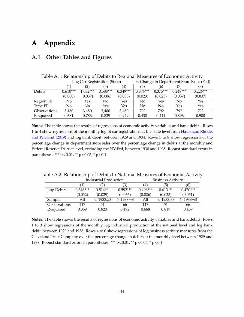
A Appendix

A.1 Other Tables and Figures

Table A.1: Relationship of Debits to Regional Measures of Economic ActivityLog Car Registration (State) % Change in Department Store Sales (Fed)

(1) (2) (3) (4) (5) (6) (7) (8)Debits 0.610*** 1.032*** 0.588*** 0.349*** 0.376*** 0.375*** 0.248*** 0.226***

(0.008) (0.037) (0.006) (0.053) (0.023) (0.023) (0.037) (0.037)Region FE No Yes No Yes No Yes No YesTime FE No No Yes Yes No No Yes YesObservations 3,480 3,480 3,480 3,480 792 792 792 792R-squared 0.681 0.786 0.839 0.929 0.438 0.441 0.896 0.900

Notes: The table shows the results of regressions of economic activity variables and bank debits. Rows1 to 4 show regressions of the monthly log of car registrations at the state level from Hausman, Rhode,and Wieland (2019) and log bank debit, between 1929 and 1934. Rows 5 to 8 show regressions of thepercentage change in department store sales over the percentage change in debits at the monthly andFederal Reserve District level, excluding the NY Fed, between 1930 and 1935. Robust standard errors inparentheses. *** p<0.01, ** p<0.05, * p<0.1

Table A.2: Relationship of Debits to National Measures of Economic ActivityIndustrial Production Business Activity

(1) (2) (3) (4) (5) (6)Log Debits 0.346*** 0.514*** 0.592*** 0.496*** 0.613*** 0.470***

(0.032) (0.029) (0.066) (0.026) (0.035) (0.051)Sample All < 1933m3 ≥ 1933m3 All < 1933m3 ≥ 1933m3Observations 117 51 66 117 51 66R-squared 0.359 0.823 0.492 0.668 0.817 0.457

Notes: The table shows the results of regressions of economic activity variables and bank debits. Rows1 to 3 show regressions of the monthly log industrial production at the national level and log bankdebit, between 1929 and 1938. Rows 4 to 6 show regressions of log business activity measures from theCleveland Trust Company over the percentage change in debits at the monthly level between 1929 and1938. Robust standard errors in parentheses. *** p<0.01, ** p<0.05, * p<0.1

44

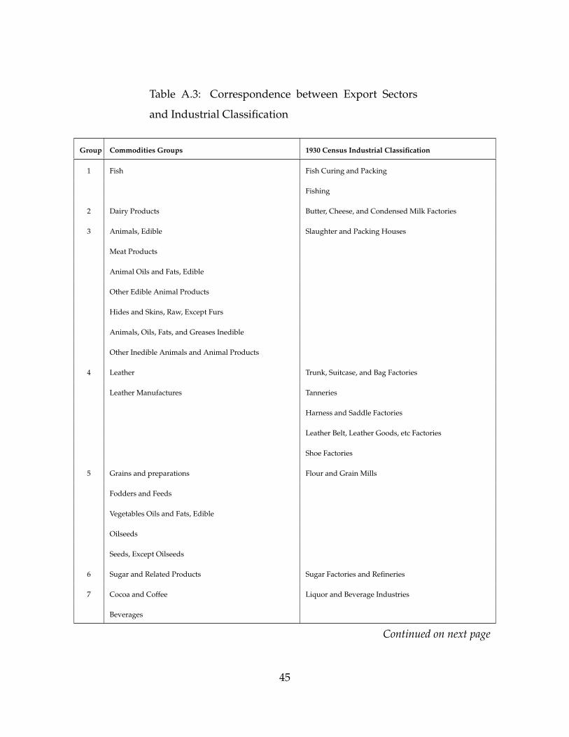
Table A.3: Correspondence between Export Sectors

and Industrial Classification

Group Commodities Groups 1930 Census Industrial Classification

1 Fish Fish Curing and Packing

Fishing

2 Dairy Products Butter, Cheese, and Condensed Milk Factories

3 Animals, Edible Slaughter and Packing Houses

Meat Products

Animal Oils and Fats, Edible

Other Edible Animal Products

Hides and Skins, Raw, Except Furs

Animals, Oils, Fats, and Greases Inedible

Other Inedible Animals and Animal Products

4 Leather Trunk, Suitcase, and Bag Factories

Leather Manufactures Tanneries

Harness and Saddle Factories

Leather Belt, Leather Goods, etc Factories

Shoe Factories

5 Grains and preparations Flour and Grain Mills

Fodders and Feeds

Vegetables Oils and Fats, Edible

Oilseeds

Seeds, Except Oilseeds

6 Sugar and Related Products Sugar Factories and Refineries

7 Cocoa and Coffee Liquor and Beverage Industries

Beverages

Continued on next page

45

Table A.3 – Continued from previous page

Group Commodities Groups 1930 Census Industrial Classification

8 Tobacco and Manufactures Cigar and Tobacco Factories

Agriculture (Tobacco)

9 Rubber and Manufactures Rubber Factories

10 Fruits and Nuts Agriculture (No Cotton-Tobacco)

Vegetables and Preparations

Drugs, Herbs, Leaves and Roots Crude

Nursery and Greenhouse Stock

Miscellaneous Vegetable Products

11 Silk manufactures Silk Mills

12 Rayon and other Synthetic Textiles Rayon Factories

Hat Factories (felt)

13 Furs and Manufactures Corset Factories

Dyeing and Tanning Materials Other and Not Specified Textile Mills

Cotton Manufactures Shirt, Collar, and Cuff Factories

Wool Manufactures Glove Factories

Silk Unmanufactures Carpet Mills

Lace and Embroidery Mills

Straw Factories

Button Factories

Sail, Awning, and Tent Factories

Other Clothing Factories

Broom and Brush Factories

Textile Dyeing, Finishing, and Printing Mills

Suit, Coat, and Overall Factories

Knitting Mills

Continued on next page

46

Table A.3 – Continued from previous page

Group Commodities Groups 1930 Census Industrial Classification

14 Cotton, Unmanufactured Cotton Mills

Cotton Semimanufactures Agriculture (Cotton)

15 Jute and Manufactures Hemp, Jute, and Linen Mills

Flax, Hemp and Ramie Manufactures Rope and Cordage Factories

Other Vegetable Fibers and Manufactures

16 Wool, Semimanufactures Woolen and Worsted Mills

Wool,

Mohair, and Angora Rabbit Hair, Unmanufactured

17 Wood, Unmanufactured Forestry

Naval Stores, Gums, and Resins

Cork and Manufactures

18 Wood manufactures Wagon and Carriage Factories

Other Woodworking Factories

Furniture Factories

19 Wood Semimanufactures-Sawmill Products Saw and Planning Mills

20 Paper and Manufactures Paper Box Factories

Blank Nook, Envelope, Tag, Paper Bag, etc. Factories

21 Paper Base Stocks Paper and Pulp Mills

22 Coal and Related Fuels Coal Mines

Charcoal and Code Works

23 Stone, Sand, Cement and Lime Quarries

Lime, Cement, and Artificial Stone Factories

24 Petroleum and Products Petroleum Refineries

Oil Wells and Gas Wells

25 Glass and Glass Products Glass Factories

26 Clays and Clay Products Potteries

Continued on next page

47

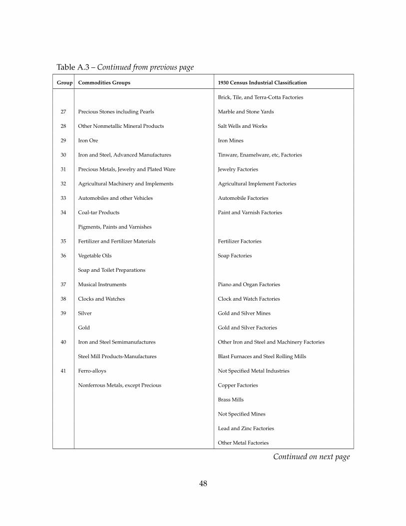
Table A.3 – Continued from previous page

Group Commodities Groups 1930 Census Industrial Classification

Brick, Tile, and Terra-Cotta Factories

27 Precious Stones including Pearls Marble and Stone Yards

28 Other Nonmetallic Mineral Products Salt Wells and Works

29 Iron Ore Iron Mines

30 Iron and Steel, Advanced Manufactures Tinware, Enamelware, etc, Factories

31 Precious Metals, Jewelry and Plated Ware Jewelry Factories

32 Agricultural Machinery and Implements Agricultural Implement Factories

33 Automobiles and other Vehicles Automobile Factories

34 Coal-tar Products Paint and Varnish Factories

Pigments, Paints and Varnishes

35 Fertilizer and Fertilizer Materials Fertilizer Factories

36 Vegetable Oils Soap Factories

Soap and Toilet Preparations

37 Musical Instruments Piano and Organ Factories

38 Clocks and Watches Clock and Watch Factories

39 Silver Gold and Silver Mines

Gold Gold and Silver Factories

40 Iron and Steel Semimanufactures Other Iron and Steel and Machinery Factories

Steel Mill Products-Manufactures Blast Furnaces and Steel Rolling Mills

41 Ferro-alloys Not Specified Metal Industries

Nonferrous Metals, except Precious Copper Factories

Brass Mills

Not Specified Mines

Lead and Zinc Factories

Other Metal Factories

Continued on next page

48

Table A.3 – Continued from previous page

Group Commodities Groups 1930 Census Industrial Classification

Copper Mines

Lead and Zinc Mines

Other Specific Mines

42 Electrical Machinery and Apparatus Electrical Machinery and Supply Factories

Industrial Machinery

43 Office Appliances Other Miscellaneous Manufacturing Industries

Printing Machinery

44 Medicinal and Pharmaceutical Preparations Other Chemical Factories

Industrial Chemicals Specialties

Industrial Chemicals

45 Explosives, Fuses, etc. Explosives, Ammunition, and Fireworks Factories

Firearms and Ammunition

Notes: The table contains the correspondence between export sectors and industrial sectors. The classifi-

cation of export sectors is the one used in the Statistical Abstract of the United States Foreign Commerce

1935. The classification of industrial sectors corresponds to the 1930 census industrial classification sys-

tem.

49

Table A.4: Exports by Commodities Groups

Commodities Groups Exports Share 32A-33M (%) Growth Rate 33M-34M (%)Group 00. Animal and animal products, edible 4.6 20.1Animal oils and fats, edible 2.4 2.1Meat products 1.3 62.71Group 0. Animals and animal products, inedible 2.3 44.0Group 1. Vegetable food products and beverages 10.6 -4.1Fruits and nuts 4.9 13.3Grains and preparations 3.9 -34.9Group 2. Vegetable products, inedible, except fibers and wood 7.7 33.6Tobacco and manufactures 5.0 36.8Rubber and manufactures 1.1 27.7Group 3. Textiles 25.7 38.2Cotton, unmanufactured 21.4 46.1Cotton manufactures 2.5 -9.6Group 4. Wood and paper 3.8 39.1Wood semimanufactures-sawmill products 1.8 46.7Paper and manufactures 1.0 10.6Group 5. Nonmetallic mineral products 18.5 10.4Petroleum and products 13.9 7.5Coal and related fuels 2.9 4.8Other nonmetallic mineral products 1.1 49.9Group 6. Metals and manufactures, except machinery and vehicles 5.5 71.6Nonferrous metals, except precious 2.1 55.5Iron and steel semimanufactures 1.0 157.8Group 7. Machinery and vehicles 14.1 36.7Automobiles and other vehicles 6.1 50.0Industrial machinery 3.8 21.8Electrical machinery and apparatus 2.7 28.7Office appliances 1.0 27.8Group 8. Chemicals and related products 4.8 19.88Industrial chemicals 1.0 28.0Group 9. Miscellaneous 4.2 -3.1Miscellaneous articles 1.5 -9.2

Notes: The table shows the share of exports between April 1932 and March 1933 and the growth betweenApril 1934 and March 1932 and between April 1932 and March 1933. The table selects sectors with ashare of total exports, excluding gold and silver, higher than 1 percent.

Figure A.1: Exports and Imports

010

020

030

040

0M

illion

s of

Dol

lars

in J

anua

ry 1

928

1928m1 1930m1 1932m1 1934m1 1936m1Date

Manufacturing Exports Manufacturing ImportsVertical lines are start of Great Depression and end of Gold Standard

Millions of DollarsManufacturing Exports and Imports

100

200

300

400

500

Milli

ons

of D

olla

rs in

Jan

uary

192

8

1928m1 1930m1 1932m1 1934m1 1936m1Date

Total Exports Total ImportsVertical lines are start of Great Depression and end of Gold Standard

Millions of DollarsTotal Exports and Imports

50

A.2 A Model of the Gold Standard and Trade

In this section, we show how the external sector adjusts in fixed and flexible exchange

rate regimes after local shocks. The model aims to shed light on the mechanism be-

hind the effect that a depreciation could have after abandoning a fixed exchange rate

regime. The model is a standard two country, multi-sector New Keynesian model with

sticky prices, where countries might engage in a fixed exchange rate. Households face

the following lifetime utility function:

∞

∑k=0

βt+kUj,t+k =∞

∑k=0

βt+kC1−γ

j,t+k

1− γ−

L1+αj,t+k

1 + α,

where j = H, F denotes the home and foreign country, β is the intertemporal dis-

count factor, γ is the intertemporal elasticity of substitution and α is one over the

Frisch elasticity of labor supply. The total labor supply of country j in time t is Lj,t =∫ 10 Lj,T,t(z)dz +

∫ 10 Lj,NT,t(z)dz where

∫ 10 Lj,T,t(z)dz and

∫ 10 Lj,NT,t(z)dz denote the labor

supply in the tradable (T) and nontradable (NT) sector, respectively. The consumption

bundle of country j, Cj,t, is composed of a tradable bundle Cj,T,t and a nontradable

bundle Cj,NT,t as

Cj,t =

[φ

1ν C

ν−1ν

j,T,t + (1− φ)1ν C

ν−1ν

j,NT,t

] νν−1

,

where φ represents the preferences for tradable goods and ν is the elasticity of substi-

tution between tradable and nontradable goods. The tradable bundle is defined as

Cj,T,t =

[φ

1σT C

σ−1σ

jj,t + (1− φT)1σ C

σ−1σ

jj′,t

] σσ−1

,

where Cjj,t is the bundle of tradable goods produced locally and Cjj′,t is the bundle of

tradable goods imported. φT denotes the preferences for local tradable goods. σ mea-

sures the substitutability between local tradable goods and imported goods. The local

tradable bundle, imported bundle, and nontradable bundle consist of a CES consump-

51

tion bundle of a continuum of producers with a common elasticity of substitution η:

Cjj,t =

[∫ 1

0Cjj,t(z)

η−1η dz

] ηη−1

Cjj′,t =

[∫ 1

0Cjj′,t(z)

η−1η dz

] ηη−1

Cj,NT,t =

[∫ 1

0Cj,NT,t(z)

η−1η dz

] ηη−1

where z ∈ [0, 1] denotes good variety. Consumers face the following budget constraint:

Wj,tLj,t + Πj,t + Bjj,t−1Rj,t−1 = Bjj,t + Pj,tCj,t,

where Wj,t is the local wage, Bjj,t is the local riskless bond, Rj,t ≡ (1 + ij,t) is the local

gross return that pays an interest rate ij,t and Πj,t are the profits of the domestic firms.

Pj,t is the local price index, defined as

Pj,t =[φP1−ν

j,T,t + (1− φ)P1−νj,NT,t

] 11−ν ,

where Pj,T,t is the price index for tradable goods consumed locally, defined as

Pj,T,t =

[φTP1−σ

jj,t + (1− φT)(Ej,tPj′ j′,t

)1−σ] 1

1−σ

,

where Ej,t = 1/Ej′,t is the exchange rate that the local consumer must pay to buy a

foreign good and Pjj,t denotes the price index for tradable goods produced in country j:

Pjj,t =

[∫ 1

0Pjj,t(z)1−ηdz

] 11−η

.

Pj,NT,t is the price index for nontradable goods:

52

Pj,NT,t =

[∫ 1

0Pj,NT,t(z)1−ηdz

] 11−η

.

An important value will be the terms of trade. We define the terms of trade as

Qj,t =Pj′ j′

PjjEj,t.

The terms of trade represent how expensive local tradable goods are, compared

with foreign tradable goods from consumers’ point of view. In this sense, a reduction in

the terms of trade implies that for the local consumer, buying imported goods is more

convenient. A similar argument can be made for the foreign consumer. Therefore, a re-

duction in the terms of trade implies that the local tradable good loses competitiveness.

We have that the uncovered interest parity condition holds, meaning that

iH,t − iF,t = EteH,t+1 − eH,t,

where ij,t is the interest rate in j and et is the log-linearized exchange rate. Finally, the

risk-sharing condition holds. We have:

(CH,t

CF,t

)γ

= ϑ0EtPF,t

PH,t.

Countries are symmetric. We assume that initially countries have the same wealth,

meaning that ϑ0 = 1.

We have also two types of firms in each country that produce each variety of the

tradable and nontradable good. Each firm has a linear production function that de-

pends on labor and a productivity term that is common across sectors Aj,t. Defining

Yj,s,t(i) as the output of the firm producing the variety i, in country j and sector s, and

Lj,s,t(i) as its labor demand, the production function is:

Yj,s,t(i) = Aj,tLj,s,t(i)

53

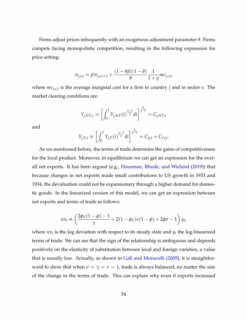
Firms adjust prices infrequently with an exogenous adjustment parameter θ. Firms

compete facing monopolistic competition, resulting in the following expression for

price setting:

πj,s,t = βπj,s,t+1 +(1− θβ)(1− θ)

θ

11 + η

mcj,s,t,

where mcj,s,t is the average marginal cost for a firm in country j and in sector s. The

market clearing conditions are:

Yj,NT,t ≡[∫ 1

0Yj,NT(i)

η−1η di

] ηη−1

= Cj,NT,t

and

Yj,T,t ≡[∫ 1

0Yj,T(i)

η−1η di

] ηη−1

= Cjj,t + Cj′ j,t.

As we mentioned before, the terms of trade determine the gains of competitiveness

for the local product. Moreover, in equilibrium we can get an expression for the over-

all net exports. It has been argued (e.g., Hausman, Rhode, and Wieland (2019)) that

because changes in net exports made small contributions to US growth in 1933 and

1934, the devaluation could not be expansionary through a higher demand for domes-

tic goods. In the linearized version of this model, we can get an expression between

net exports and terms of trade as follows:

nxt ∝(

2φT(1− φ)− 1γ

+ 2(1− φT)ν(1− φ) + 2φσ− 1)

qt,

where nxt is the log deviation with respect to its steady state and qt the log-linearized

terms of trade. We can see that the sign of the relationship is ambiguous and depends

positively on the elasticity of substitution between local and foreign varieties, a value

that is usually low. Actually, as shown in Gali and Monacelli (2005), it is straightfor-

ward to show that when σ = γ = ν = 1, trade is always balanced, no matter the size

of the change in the terms of trade. This can explain why even if exports increased

54

sharply after the depreciation of 1933, net exports increased only mildly in 1933. We

can also show that local consumption is positively related to the terms of trade:

CH,t = CF,t +2γ

φT(1− φ)qt.

Finally, there are two regimes of monetary policy. The first is the fixed exchange

rate regime that comes from the gold standard. In that case, we assume that the nom-

inal product is equal to a monetary mass that is equal to the world supply of gold. At

the same time, this regime implies a fixed exchange rate, given by

PgMt = PH,tYH,t + PF,tYF,t

and

Et = 1,

where Mt is the world supply of gold that we take as constant, the same as the price of

gold Pg. All countries have the same gold rule, so equalizing the rule everywhere im-

plies a fixed exchange rate. In the second regime, each country has its own monetary

policy rule, given by

iH,t = φππH,t + φyyH,t

and

iF,t = φππF,t + φyyF,t,

with φπ and φy the weights on the monetary decision for inflation and output. In both

regimes the uncovered interest parity holds. We start evaluating the effect of a local

negative productivity shock in country H comparing both regimes. We calibrate the

data using β = 0.99, α = 1.0, η = 7, ρ = 0.9, γ = 1, θ = 0.7, φπ = 1.5, φy = 1.0, φ = 0.7,

φT = 0.7, ν = 6 and χ = 4. Figure A.2 compares the dynamics of the economy under

55

both regimes.

Figure A.2: Productivity Shock under Fixed and Flexible Exchange Rates

0 10 20 30 40-0.4

-0.2

0

0.2

0.4Tradable Output

FixedFlexible

0 10 20 30 40-0.4

-0.2

0

0.2

0.4Non-Tradable Output

FixedFlexible

0 10 20 30 40-1

-0.5

0

0.5

1Exports

FixedFlexible

0 10 20 30 40-5

0

5Exchange Rate

FixedFlexible

0 10 20 30 40-0.3

-0.2

-0.1

0

0.1

0.2

0.3

Terms of Trade

FixedFlexible

Notes: The figure shows an impulse response from a 1 percent negative productivity shock in the homeeconomy for tradable output, nontradable output, exports, the nominal exchange rate, and the terms oftrade in the home economy as defined in the paper. The dashed line represents the impulse response ina flexible exchange rate regime and the solid-dot line represents it under the fixed exchange rate regime.

We can see that under the flexible exchange rate regime the recovery is much faster.

Moreover, the contraction of tradable and nontradable output is smaller. Under the

fixed exchange rate, the terms of trade decrease much more following a negative pro-

ductivity shock, which depresses the external sector, as we can see in the decrease in

exports. In the flexible regime, the exchange rate depreciates immediately, buffering

the reduction in the terms of trade. This creates a gain in competitiveness compared

with the fixed exchange rate. This adjustment in relative prices permits an increase in

demand for locally produced goods that keeps tradable output relatively high and also

increases demand for nontradable goods.

When there is a fixed exchange rate the whole economy is more recessive and the

56

recession lasts more. In the empirical part of this paper, we will evaluate two regime

changes. We can use the model to inform how the transition will be. For that, we sim-

ulate the negative local productivity shock and after 8 periods we release the interest

rate, moving toward the flexible exchange rate. This change in regime is unexpected.

Figure A.3 shows the reaction in terms of output, exports, and the exchange rate.

Figure A.3: Productivity shock With Change in Regime

0 10 20 30 40-0.4

-0.2

0

0.2

0.4Tradable Output

0 10 20 30 40-0.4

-0.2

0

0.2

0.4Non-Tradable Output

0 10 20 30 40-1

-0.5

0

0.5

1Exports

0 10 20 30 40-3

-2

-1

0

1

2

3Exchange Rate

0 10 20 30 40-0.3

-0.2

-0.1

0

0.1

0.2

Terms of Trade

Notes: The figure shows an impulse response from a 1 percent negative productivity shock in the homeeconomy for tradable output, nontradable output, exports, the nominal exchange rate, and the termsof trade. Until the eighth period, the economy is under the fixed exchange rate regime. After that, theeconomy unexpectedly switches to a flexible exchange rate regime.

When there is a change in regime we see that the model predicts some very sim-

ilar figures compared with the empirical facts we will show below. Exports increase

strongly after the change in the exchange rate regime. This is produced by an increase

in the terms of trade when the regime is changed. We can see that this also produces a

strong recovery in the tradable sector, which also pushes up the nontradable sector.

This model allows us to find some margins along which to evaluate the effect of the

57

change in the exchange rate regime. From the data and the model, we see a currency

depreciation and an increase in exports after the change in regime. The increase in ex-

ports is not complete in the data, as it represents a shift to a new path of convergence.

Empirically we can still evaluate other margins that are important in the model.

A.2.1 Log-linearization

The log-linearized solution is given by the following equations (for simplicity, all the

variables in lower case represent log changes):

πH,T,t = βπH,T,t+1 +(1− θβ)(1− θ)

θ

11 + η

mcH,T,t

πF,T,t = βπF,T,t+1 +(1− θβ)(1− θ)

θ

11 + η

mcF,T,t

πH,NT,t = βπH,NT,t+1 +(1− θβ)(1− θ)

θ

11 + η

mcH,NT,t

πF,NT,t = βπF,NT,t+1 +(1− θβ)(1− θ)

θ

11 + η

mcF,NT,t

cF,t = −1γ(iF,t − EtπF,t+1) + EtcF,t+1

iH,t − iF,t = Etet+1 − et

pH,T,t = φpHH,t + (1− φ)(pFF,t + et)

pF,T,t = φpFF,t + (1− φ)(pHH,t − et)

pH,t = φT pH,T,t + (1− φT)pH,NT,t

pF,t = φT pF,T,t + (1− φT)pF,NT,t

58

πH,T,t = pHH,t − pHH,t−1

πF,T,t = pFF,t − pFF,t−1

πH,t = pH,t − pH,t−1

πF,t = pF,t − pF,t−1

pHH,t = pH,NT,t

pFF,t = pF,NT,t

mcH,T,t = (1 + α)yH,T,t +

(γ− 1

ν

)cH,t +

(1ν− 1

σ

)cH,T,t +

1σ

cHH,t − (1 + α)aH,t

mcF,T,t = (1 + α)yF,T,t +

(γ− 1

ν

)cF,t +

(1ν− 1

σ

)cF,T,t +

1σ

cFF,t − (1 + α)aF,t

mcH,NT,t = (1 + α)yH,NT,t +

(γ− 1

ν

)cH,Nt +

(1ν− 1

σ

)cH,NT,t − (1 + α)aH,t

mcF,NT,t = (1 + α)yF,NT,t +

(γ− 1

ν

)cF,t +

(1ν− 1

σ

)cF,BT,t − (1 + α)aH,t

cFH,t − cFF,t = σ(pFF,t + et − pHH,t)

59

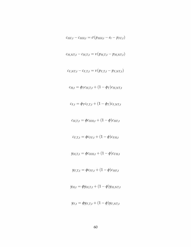
cHF,t − cHH,t = σ(pHH,t − et − pFF,t)

cH,NT,t − cH,T,t = ν(pH,T,t − pH,NT,t)

cF,NT,t − cF,T,t = ν(pF,T,t − pF,NT,t)

cH,t = φTcH,T,t + (1− φT)cH,NT,t

cF,t = φTcF,T,t + (1− φT)cF,NT,t

cH,T,t = φcHH,t + (1− φ)cHF,t

cF,T,t = φcFF,t + (1− φ)cFH,t

yH,T,t = φcHH,t + (1− φ)cFH,t

yF,T,t = φcFF,t + (1− φ)cHF,t

yH,t = φyH,T,t + (1− φ)yH,NT,t

yF,t = φyF,T,t + (1− φ)yF,NT,t

60

yH,NT,t = cH,NT,t

yF,NT,t = cF,NT,t

aH,t = ρaH,t−1 + εH,t

aF,t = ρaF,t−1 + εF,t

A.2.2 Fixed Exchange Rate Regime

et = 0

M = pH,t + yH,t + pF,t + yF,t

A.2.3 Nominal Exchange Rate Regime

iH,t = φππH,t + φyyH,t

iF,t = φππF,t + φyyF,t

61