benchmarks and performance tests - pearson...

Chapter 7

BenchmarksandPerformanceTests

7.1 Introduction

It’s common sense—everyone agrees that the best way to study the per-

formance of a given system is to run the actual workload on the hardware

platform and measure the results. However, many times this approach is not

feasible.

Here are two situations where one needs to take alternate approaches

to study the performance of a system. The first case is that of a company

that is planning to roll out a new Web-based order system. Management

has already specified the software architecture and is about to start the

procurement process to select the server systems. The performance analyst

261

Prentice Hall PTR

This is a sample chapter of Capacity Planning for Web Services: Metrics, Models, and Methods ISBN: 0-13-065903-7 For the full text, visit http://www.phptr.com ©2001 Pearson Education. All Rights Reserved.

262 Benchmarks and Performance Tests Chapter 7

understands that it is not either viable or cost-effective to set up configura-

tions of Web servers to run pieces of the actual workload and measure their

performance. Therefore, the analyst decided to use standard benchmark re-

sults. Benchmarking is the primary method for measuring the performance

of an actual physical machine [7]. Benchmarking refers to running a set of

representative programs on different computers and networks and measuring

the results. Benchmark results are used to evaluate the performance of a

given system on a well-defined workload. Much of the popularity of standard

benchmarks comes from the fact that they have performance objectives and

workloads that are measurable and repeatable. Usually, computer system

procurement studies and comparative analyses of products rely on bench-

marks. They are also used as monitoring and diagnostic tools. Vendors,

developers, and users run benchmarks to pinpoint performance problems of

new systems.

Consider now an online brokerage’s trading site that is planning a major

change in the services it provides on the Internet. The application is ready for

deployment and the engineers are prepared to put the code on the live site.

But management is cautious about this procedure and wants to make sure

its customers will not face unpleasant surprises when accessing the new site.

Management is concerned about scalability problems and is not sure if the

site can handle heavy traffic loads. In other words, management wants to do

predictive testing rather than reacting to failures. The most commonly used

approach to obtain performance results of a given Web service is performance

testing, which means to run tests to determine the performance of the service

under specific application and workload conditions. In the Web environment,

companies cannot afford to deploy services and applications before ensuring

that they run really well. It is crucial to predict how a particular Web

service will respond to a specific workload. Benchmarks are not able to

provide accurate answers to questions about specific scenarios of workload

and applications. Therefore, one has too look for specific performance tests.

Based on a particular workload and application scenario, performance testing

Section 7.2 The Nature of Benchmarks 263

should provide information on how the service will respond to realistic loads

before it goes into production.

This chapter presents several different standard industry benchmarks and

discusses them in the context of performance modeling and capacity plan-

ning. It also shows a methodology for performance testing, that follows the

various steps of the capacity planning methodology introduced in Chapter 5.

7.2 The Nature of Benchmarks

Time and rate are the basic measures of system performance. From the

user’s viewpoint, program or application execution time is the best indicator

of system performance. Users do not want to know if the service is executed

next to the desktop computer on the LAN or if it is processed thousands

of miles away from her/his location, connected through various networks.

Users always want fast response time. From management’s viewpoint, the

performance of a system is defined by the rate at which it can perform

work. For example, system managers are interested in questions such as:

How many transactions can the system execute per minute, or how many

requests is the Web site able to service per second? In addition, both users

and managers are always concerned with cost, reflected in questions such

as: What is the system’s operational cost? And what is the server purchase

cost? As a consequence of all these different viewpoints, the basic problem

remains: What is a good standard measure of system performance?

Computer makers usually refer to the speed of a processor by its cycle

time, which can be expressed by its length (e.g., 1 nanosecond) or by its rate

(e.g., 1 GHz). However, one common misperception is the use of the clock

speed (i.e., in gigahertz or nanoseconds) to compare processor performance.

The overall performance of a processor is directly affected by other archi-

tectural traits, such as caching, pipelining, functional units and compiler

technology [5]. In the past, a popular way of rating processor performance

was MIPS (millions of instructions per second). Although MIPS had been


largely employed as a basis for comparisons of processors, it is important

to remind the reader about the problems with its use. MIPS is dependent

on the instruction set, which makes it difficult to compare computers with

different repertoires of instructions. For instance, using MIPS to compare

the performance of a Reduced Instruction Set Computer (RISC) with that

of a Complex Instruction Set Computer (CISC) has little significance. As

MIPS is not defined in a domain of any specific application, its use may be

misleading. Different programs running on the same computer may reach

different levels of MIPS.

System performance is complex; it is the result of the interplay of many

hardware and software components. Compounding the problem is the fact

that every Web service architecture is unique in its configuration, applica-

tions, operating systems, and workload. Furthermore, Web services exhibit

a large variation in performance when running different workloads. No single

number can represent the performance of a Web system on all applications.

In a quest to find a good performance measure, standard programs, known

as benchmarks, have been used to evaluate the performance of systems.

Benchmark results can both inform and confuse users about the real

capability of systems to execute their actual production workloads. The

source of confusion lies on how one interprets benchmark results. Before

using benchmark results, one must understand the workload, the system

under study, the tests, the measurements, and the results. Otherwise, one

will not be able to interpret the benchmark results properly. Therefore, the

first step is to answer the following questions.

• What is a particular benchmark actually testing?

• How close does the benchmark resemble the user environment work-

load?

• What is the benchmark really measuring?

Once benchmark results are well understood, one can use them to increase


one’s knowledge about the performance of the system under study. For

example, benchmark results can be used to estimate input parameters for

performance models of Web service environments. Or they can give an

idea about the performance of a system when processing heavy workloads.

However, it is important to note that most benchmarks are good tools for

comparing systems, rather than accurate tools for sizing or capacity planning

for a given Web service.

7.2.1 Benchmark Hierarchy

Benchmarks can be viewed as grouped into two categories: coarse-grain

benchmarks and fine-grain benchmarks [7]. The granularity of the bench-

mark is determined by the granularity of the property that can be measured

by the benchmark. For example, a benchmark measuring the performance of

an e-commerce system is considered coarse-grain, while a benchmark mea-

suring the CPU speed is considered fine-grain. A series of complex tests,

of different granularities, has been designed to investigate the performance

of computer systems. The plethora of existing benchmark programs can be

thought of as a hierarchy, where different levels are characterized by the

complexity and granularity of their tests as well as by their ability to predict

actual performance.

At the innermost level of the hierarchy, as shown in Fig. 7.1, are syn-

thetic benchmarks that perform only basic operations, such as addition and

multiplication. Dhrystone is an example of this type of program: It is a syn-

thetic benchmark aimed at measuring the speed of a system when executing

fixed-point computations. This type of program does not compute any real

task and its utility to the comprehension of performance of practical systems

is very limited.

At the second level of the benchmark hierarchy are the so-called toy

benchmarks. They are very small programs that implement some classical

puzzles, such as Sieve of Eratosthenes and Towers of Hanoi [5]. These types


Basicoperations

ComputerSystems

Realprograms

PerformanceMeasures

Kernels Benchmark"Toy"

Figure 7.1. Benchmark hierarchy.

of benchmark are not helpful in predicting the performance of real workloads

and have no use in the analysis of practical problems.

Kernels, the third level, are portions of code extracted from real pro-

grams. These pieces of code represent the essence of the computation, i.e.,

where most of the time is spent. Livermore Loops and Linpack are good

examples of program kernels. In general, this type of benchmark concen-

trates on the system’s capability to execute some numeric computation and

therefore measures only the processor performance. Because they are not

real programs, they provide little information about the performance per-

ceived by end users. At the outermost level of the hierarchy is the workload

composed of full-scale, real programs used to solve real problems. These

programs make up benchmark suites, such as SPEC, and TPC. As an ex-

ample, there are some domain-oriented benchmarks that use programs such

as components of the C programming language compiler, word processing,

and debit and credit bank transactions. They offer useful information about

the performance of a given system when running some given applications.


7.2.2 Avoiding Pitfalls

As in any performance study, the first step to safely interpret the benchmark

results is to understand the environment (see Chapter 5). In other words,

one needs to know where and how the benchmark tests were carried out.

Basically, one needs information such as processor specification (e.g., model,

cache, and number of processors), memory, I/O subsystem (e.g., disks, mod-

els, and speed), network (e.g., LAN, WAN, and operational conditions), and

software (e.g., operating system, compilers, transaction processing monitor,

and database management system). Once you understand the benchmark

environment, then you should consider several other factors before making

use of the benchmark numbers. To avoid pitfalls, you should ask yourself

some key questions to find out how relevant the benchmark results are to

your particular system or application. Examples of these key questions are:

• Does the SUT have a configuration similar to the actual system? Ex-

amine the configuration description and compare the hardware, the

network environment (topology, routers, protocols, and servers), the

software, the operating system parameters, and the workload. Does

the testing environment look like my system environment? Is the num-

ber of processors in your system the same as that described in the

benchmark environment? What version of the OS was used in the

tests? What were the memory and cache sizes of the server? These

are typical questions you should answer before drawing conclusions

about the benchmark results.

• How representative of the actual workload are the benchmark tests?

For example, if your system is dedicated to order processing, then

a transaction processing benchmark can give you some insight about

the performance of your application. However, if you are planning a

new graphical application, transaction processing benchmark results

are useless, because the two workloads are very dissimilar.


As systems evolve, so must the benchmarks that are used to compare them.

All standard benchmarks release new versions periodically. Therefore, when

examining benchmark results, pay attention to the version used and look for

new features included in the latest releases.

7.2.3 Common Benchmarks

Many benchmark tests are used to evaluate a wide variety of systems, subsys-

tems, and components under different types of workloads and applications.

Users groups and searches on the Web are good sources of updated informa-

tion about several types of benchmarks. However, to be useful, a benchmark

should have the following attributes [4]:

• Relevance: It must provide meaningful performance measures within

a specific problem domain.

• Understandable: The benchmark results should be simple and easy to

understand.

• Scalable: The benchmark tests must be applicable to a wide range of

systems, in terms of cost, performance, and configuration.

• Acceptable: The benchmarks should present unbiased results that are

recognized by users and vendors.

Two consortia offer benchmarks that are common yardsticks for comparing

different computer systems. The System Performance Evaluation Corpora-

tion (SPEC) [11] is an organization of computer industry vendors that devel-

ops standardized performance tests, i.e., benchmarks, and publishes reviewed

results. SPEC publishes benchmark performance results of CPU, multipro-

cessor systems, file server, mail server, Web server, and graphics [11]. The

Transaction Processing Performance Council (TPC) [15] is a nonprofit or-

ganization that defines transaction processing, database, and e-commerce

benchmarks. TPC-C, TPC-H, TPC-R are commonly used industry bench-

Section 7.3 Processor Benchmarks 269

marks that measure throughput and price/performance of OLTP environ-

ments and decision support systems [4] and TPC-W measures the perfor-

mance of systems that deliver e-commerce service. The next sections discuss

characteristics of various standard benchmarks.

7.3 Processor Benchmarks

SPEC CPU benchmark is designed to provide measures of performance

for comparing compute-intensive workloads on different computer systems.

SPEC CPU benchmarks are designated as SPECxxxx, where xxxx speci-

fies the generation of the benchmark. SPEC2000 [6] contains two suites of

benchmarks: int and fp. The former is designed for measuring and compar-

ing compute-intensive integer performance. The latter focuses on floating-

point performance. Because these benchmarks are compute-intensive, they

concentrate on the performance of the computer’s processor, the memory

architecture, and the compiler.

7.3.1 Workload

The SPEC benchmark suite consists of programs selected from various sour-

ces, primarily academic and scientific. Some are reasonably full implemen-

tations and other programs are adaptations to fulfill the benchmark goal

of measuring CPU. The fp suite for measuring floating-point compute per-

formance contains fourteen applications written in the FORTRAN and C

languages. The benchmark suite (CINT2000) that measures integer com-

pute performance comprises twelve applications written in C and C++. In

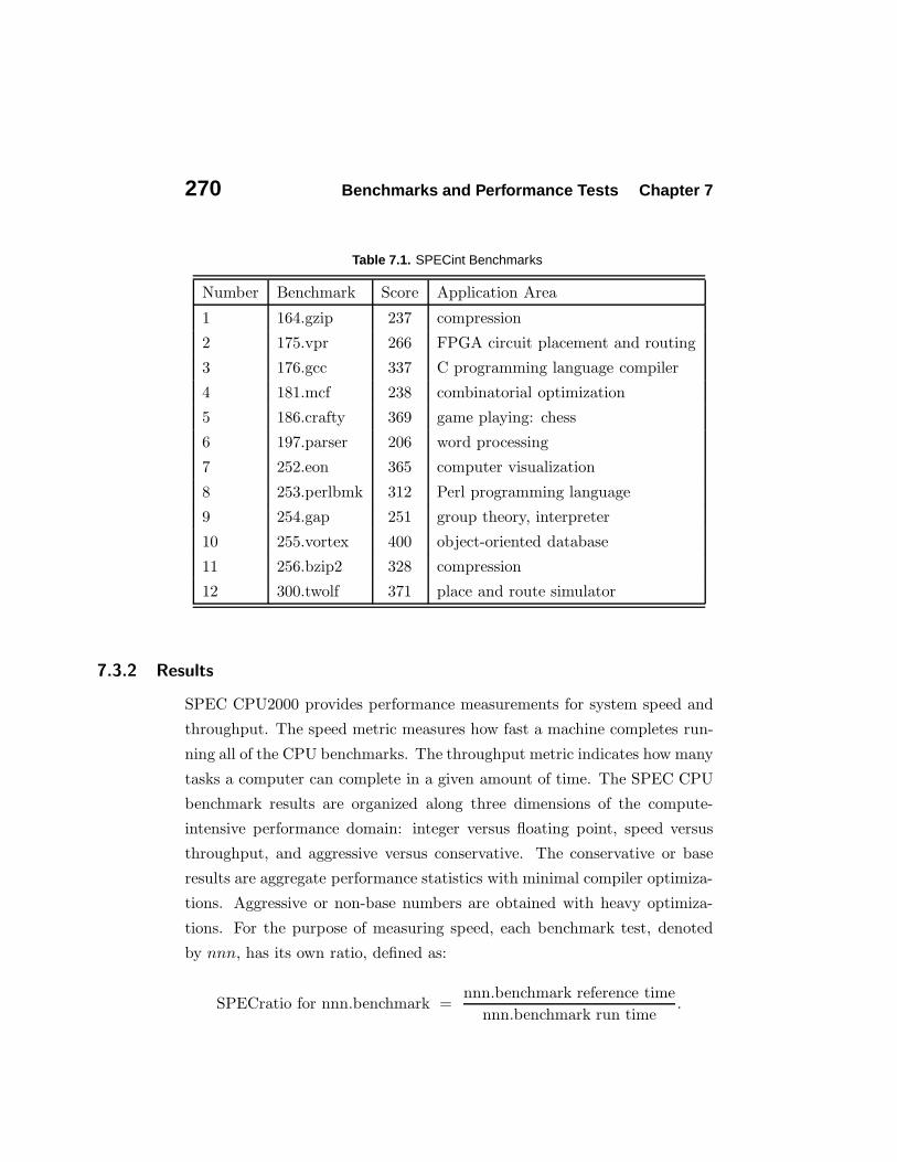
addition to the short description of the benchmarks, Table 7.1 also shows the

SPECint performance for a given machine. Performance is stated relative to

a reference machine, a 300-MHz Sun Ultra5 10, which gets a score of 100.

Each benchmark program is run and measured on this machine to establish

a reference time for that benchmark. These times are used to calculate the

SPEC results described in the next section.


Table 7.1. SPECint Benchmarks

Number Benchmark Score Application Area

1 164.gzip 237 compression

2 175.vpr 266 FPGA circuit placement and routing

3 176.gcc 337 C programming language compiler

4 181.mcf 238 combinatorial optimization

5 186.crafty 369 game playing: chess

6 197.parser 206 word processing

7 252.eon 365 computer visualization

8 253.perlbmk 312 Perl programming language

9 254.gap 251 group theory, interpreter

10 255.vortex 400 object-oriented database

11 256.bzip2 328 compression

12 300.twolf 371 place and route simulator

7.3.2 Results

SPEC CPU2000 provides performance measurements for system speed and

throughput. The speed metric measures how fast a machine completes run-

ning all of the CPU benchmarks. The throughput metric indicates how many

tasks a computer can complete in a given amount of time. The SPEC CPU

benchmark results are organized along three dimensions of the compute-

intensive performance domain: integer versus floating point, speed versus

throughput, and aggressive versus conservative. The conservative or base

results are aggregate performance statistics with minimal compiler optimiza-

tions. Aggressive or non-base numbers are obtained with heavy optimiza-

tions. For the purpose of measuring speed, each benchmark test, denoted

by nnn, has its own ratio, defined as:

SPECratio for nnn.benchmark =nnn.benchmark reference time

nnn.benchmark run time.

Section 7.3 Processor Benchmarks 271

SPECint is the geometric mean of 12 normalized ratios, one for each

benchmark program in Table 7.1. This metric refers to the benchmark re-

sults compiled with aggressive (i.e., non-base) optimizations. SPECint base

is the geometric mean of 12 normalized ratios when compiled with conser-

vative optimization for each benchmark. For each benchmark of the CINT

suite, a throughput measure is calculated. SPECint rate is the geometric

mean of twelve normalized throughput ratios. SPECint rate base is the ge-

ometric mean of twelve normalized throughput ratios when compiled with

conservative optimization for each benchmark. Similar measures are calcu-

lated for the CFP suite using the individual results obtained for each of the

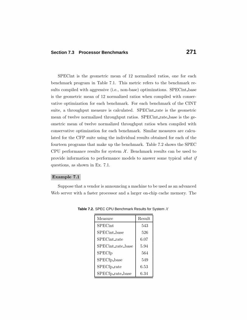
fourteen programs that make up the benchmark. Table 7.2 shows the SPEC

CPU performance results for system X . Benchmark results can be used to

provide information to performance models to answer some typical what if

questions, as shown in Ex. 7.1.

Example 7.1

Suppose that a vendor is announcing a machine to be used as an advanced

Web server with a faster processor and a larger on-chip cache memory. The

Table 7.2. SPEC CPU Benchmark Results for System X

Measure Result

SPECint 543

SPECint base 526

SPECint rate 6.07

SPECint rate base 5.94

SPECfp 564

SPECfp base 549

SPECfp rate 6.53

SPECfp rate base 6.34


vendor says that the new technology improves performance by 60%. Before

deciding on the upgrade, you want an answer to the classic question: “What

if we use the new Web server?” Although the vendor does not provide specific

information about the performance of Web services, it points to the SPECint

results. In this case, SPECint is relevant because the technology upgrade

reflects directly on the CPU speed. To estimate the new server impact on

the response time of HTTP requests, we can use the models described in

Chapter 10. However, we need to feed the model with input data that

reflect the speed of the new server. Note that the new technology basically

improves the CPU performance. The SPECint for the old and new servers

are 363 and 489, respectively. Therefore, we should change the CPU service

demands to reflect the server upgrade. Let α denote the ratio between the

SPECint of the two servers:

α =SPECintnew

SPECintold=

489

363= 1.35.

The new CPU service demand, denoted by Dnewcpu , is

Dnewcpu =

Doldcpu

α=

Doldcpu

1.35. (7.3.1)

What Eq. (7.3.1) says is that the CPU service time of the HTTP requests

will be smaller in the new processor. In other words, the CPU time dedi-

cated to service the requests should be divided by α = 1.35 to reflect the

faster processor. Although CPU is a key component of a system, the overall

system performance depends on many factors, such as I/O and networking.

Performance models, such as those described in Chapters 9 and 10, are able

to calculate the effect of upgrading the CPU on the overall performance of

the system using the new CPU demands.

7.4 Web Server Benchmarks

A set of tests and workloads are specified to measure Web servers. The

most commonly used Web server benchmarks are detailed next. This sec-

Section 7.4 Web Server Benchmarks 273

tion describes three Web server benchmarks: Webstone, SPECweb [11], and

Scalable URL Reference Generator (SURGE) [3]. Those programs simulate

Web clients. They generate requests to a server, according to some spec-

ified workload characteristics, receive the responses returned by the server

and collect the measurements. It is important to note that Web server

benchmarks are usually carried out in small, isolated LANs, with almost no

transmission errors. On the contrary, Web services, offered in real world,

are accessed through the Internet or large intranets, which involve WAN

connections, gateways, routers, bridges, and hubs that make the network

environment noisy and error-prone. Moreover, latencies are much higher

in real-world environments than in the LANs used in benchmarking efforts.

Thus, the analysis of Web benchmark results should take this observation

into account.

7.4.1 SPECweb

SPECweb is a software benchmark product developed by SPEC [11], de-

signed to measure a system’s ability to act as a Web server. SPECwebxx

specifies the generation (xx) of the Web server benchmark. SPECweb99

measures the maximum number of simultaneous connections that a Web

server is able to support while still meeting specific throughput and error

rate requirements. The standard benchmark workload includes both static

and dynamically generated HTML and support for HTTP 1.1. It can be

used to evaluate the performance of Web server software running on Posix-

compliant UNIX or Windows NT systems. SPECweb99 uses one or more

client systems to generate the HTTP workload for the server. Each client

sends HTTP requests to the server and then validates the response received.

At the end of the benchmark run, the data from all the clients is collected

by the prime client. The prime client process coordinates the test execution

of the client processes on the client machines. This client uses this data

to calculate aggregate bit rate for the test and determine the number of

simultaneous connections that conform to the specified bit rate limits.


7.4.1.1 Workload

The workload characteristics for SPECweb99 were drawn from the logs

of several popular Internet servers and some smaller Web sites. Thus,

SPECweb tries to mimic the access patterns to the documents of a server of

a typical Web service provider that supports home pages for various compa-

nies and organizations. Each home page is a collection of files ranging in size

from small icons to large documents or images. The different types of re-

quests that comprise the overall workload mix are summarized in Table 7.3.

The SPECweb workload mixes four classes of files, according to their file

sizes and access percentages, as displayed in Table 7.4. The workload file

set consists of a number of directories. Each directory contains nine files

per class, 36 files in total. Within each class, access distributions reflect the

fact that certain files are more popular than others. Accesses are generated

using the Zipf’s Law distribution. The resulting overall distribution is very

close to actual measured distributions on real servers [11]. It is worth noting

that the relationship established for file sizes and frequency in this workload

follows the heavy-tailed distribution concepts discussed in Chapter 4. The

total size of the file set of SPECweb scales with the expected throughput.

The rationale for that stems from the fact that expectations for a high-end

server, in terms of the variety and size of the documents available, are much

Table 7.3. Percentage of Requests in the SPECweb99 Workload

Request Percentage

Static GET 70.00

Standard Dynamic GET 12.45

Standard Dynamic GET (CGI) 0.15

Customized Dynamic GET 12.60

Dynamic POST 4.80


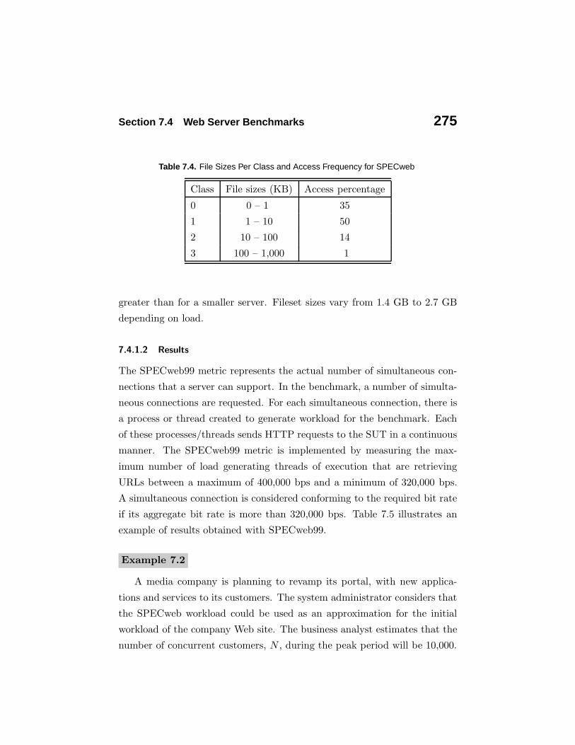
Table 7.4. File Sizes Per Class and Access Frequency for SPECweb

Class File sizes (KB) Access percentage

0 0 – 1 35

1 1 – 10 50

2 10 – 100 14

3 100 – 1,000 1

greater than for a smaller server. Fileset sizes vary from 1.4 GB to 2.7 GB

depending on load.

7.4.1.2 Results

The SPECweb99 metric represents the actual number of simultaneous con-

nections that a server can support. In the benchmark, a number of simulta-

neous connections are requested. For each simultaneous connection, there is

a process or thread created to generate workload for the benchmark. Each

of these processes/threads sends HTTP requests to the SUT in a continuous

manner. The SPECweb99 metric is implemented by measuring the max-

imum number of load generating threads of execution that are retrieving

URLs between a maximum of 400,000 bps and a minimum of 320,000 bps.

A simultaneous connection is considered conforming to the required bit rate

if its aggregate bit rate is more than 320,000 bps. Table 7.5 illustrates an

example of results obtained with SPECweb99.

Example 7.2

A media company is planning to revamp its portal, with new applica-

tions and services to its customers. The system administrator considers that

the SPECweb workload could be used as an approximation for the initial

workload of the company Web site. The business analyst estimates that the

number of concurrent customers, N , during the peak period will be 10,000.


Table 7.5. Results for SPECweb 99

System Conforming Throughput Response Kbps

Connections operations/sec msec

A 1890 5190.1 351.9 341.1

B 3222 9020.4 358.5 335.9

C 8710 24,334.1 359.6 340.2

For the purpose of planning the capacity of the service, a customer is an ac-

tive Web browser that periodically sends requests from a client machine to

the service. A customer is considered to be concurrent with other customers

as long as he or she is on the system submitting requests, receiving results of

requests, viewing the results, and submitting new requests. So, a concurrent

customer alternates between two states: viewing results (i.e., thinking) and

waiting for the response of the request (i.e., the service is busy executing the

request).

IT management agreed on defining an upper limit of 4 seconds for the

average user-perceived response time, R. In order to have a first idea about

the type and size of system needed, the capacity planning analyst used a

simple model to estimate the throughput, X0, that will be required from the

system. The business analyst estimates that the average think time, Z, for a

concurrent customer is 3 seconds. Using the Response Time Law, we have:

X0 ≥N

R + Z=

10, 000

4 + 3= 1429 requests/sec.

Now, the analyst wants to know what is the average number of simulta-

neous connections generated by the 10,000 concurrent customers. In order

to estimate this number, the analyst considered that the user-perceived re-

sponse time is composed of two components: network time and Web site

time. The analyst estimates that the network time is around 1.2 sec. There-

fore, the Web site time, Rsite, should not exceed 2.8 (= 4.0 − 1.2) seconds.


Using Little’s Law, we are able to estimate the average number of simulta-

neous connections, Nconn, as

Nconn = X0 ×Rsite = 1429 × 2.8 = 4, 001.

By examining the SPECweb benchmark results, the analyst found a

system that meets the load requirements, i.e., the number of conforming

connections is greater than 4,001 and the throughput is greater than 1429

requests/sec.

7.4.2 Webstone

Webstone is a configurable C/S benchmark for HTTP servers that uses work-

load characterization parameters and client processes to generate HTTP

traffic to stress a server in different ways [14]. It was designed to measure

maximum server throughput and average response time for connecting to

the server. It makes a number of GET requests for specific documents on

the Web server under study and collects performance data. The first version

of the benchmark did not include CGI loads or the effects of encryption or

authentication in the tests. Webstone is a distributed, multiprocess bench-

mark, composed of master and client processes. The master process, local

or remote, spawns a predefined number of client processes that start gener-

ating HTTP requests to the server. After all client processes finish running,

the master process gathers the performance summary report. The user can

either specify the duration of the test or the total number of iterations.

7.4.2.1 Workload

There are four different synthetic page mixes that attempt to model real

workloads. The characteristics of each page mix, i.e., file sizes and access

frequencies, were derived from the access patterns to pages available in some

popular Web sites. Webstone allows one to model user environment work-

loads, via synthetic loads generated according to some input parameters,

specified by the user. The specification parameters are:


• Number of clients that request pages. Clients request pages as fast as

the server can send them back. User think times cannot be represented

in the Webstone workload.

• Type of page, defined by file size and access frequency. Each page in

the mix has a weight that indicates its probability of being accessed.

• The number of pages available on the server under test.

• The number of client machines, where the client processes execute on.

Webstone 2.x offers new workloads for dynamic pages. It allows one to test

Web servers using three different types of pages: HTML, CGI and API. In

the case of API workload, Webstone comes with support for both NSAPI

and ISAPI.

7.4.2.2 Results

The main results produced by Webstone are throughput and latency. The

former, measured in bytes per second, represents the total number of bytes

received from the server divided by the test duration. Two types of latency

are reported: connection latency and request latency. For each metric, the

mean time is provided, as well as the standard deviation of all data, plus the

minimum and maximum times. Connection latency reflects the time taken

to establish a connection, while request latency reflects the time to complete

the data transfer once the connection has been established. User-perceived

latency will include the sum of connection and request latencies, plus any

network latency due to WAN connections, routers, or modems. Table 7.6

displays a summary of Webstone results for a test run of 10 minutes [14].

The Webstone number corresponds to the throughput measured in pages

per minute. The total amount of data moved is the product of the total

number of pages retrieved and the page sizes. The page size is the sum of all

files associated with the page plus the HTTP overhead in bytes. The other

results are self-explanatory.


Table 7.6. Typical Webstone Results

Metric Value

Webstone number 456

Total number of clients 24

Total number of pages retrieved from the server 4,567

Total number of errors 0

Total number of connects to server 12,099

Average time per connect (sec) 0.0039

Maximum time per connect (sec) 0.0370

Total amount of bytes moved 129,108,600

Average throughput (bytes/sec) 215,181

Average response time (sec) 1.181

Maximum response time (sec) 18.488

Webstone also presents a metric called Little’s Load Factor (LLF), de-

rived from Little’s Law [9]. It indicates the degree of concurrency on the

request execution, that is, the average number of connections open at the

Web server at any particular instant during the test. It is also an indica-

tion of how much time is spent by the server on request processing, rather

than on overhead and errors. Ideally, LLF should be equal to the number

of clients. A lower value indicates that the server is overloaded, and some

requests are not being serviced before they time out. From Chapter 3, we

know that the total number of customers in a box is equal to the throughput

of the box multiplied by the average time each customer spends in the box.

Thinking of the Web server as a box, we have that

AvgNumberOfConnections = ConnectionRate ×AvgResidenceTime.

(7.4.2)

The average residence time is the average response time plus the connection


time. Plugging numbers from Table 7.6 into Eq. (7.4.2), we have that

AvgNumberOfConnections = 12, 099/(10 × 60)× (1.181 + 0.0039) = 23.89.

In this example, the average number of connections (23.89) is very close to

the number of clients (24).

Example 7.3

Assume that the results displayed in Table 7.6 correspond to a Webstone

run with parameters configured to represent the workload forecast for the

Web site of a hotel company. The capacity planner wants to size the band-

width of the link that connects the site to the ISP. The bandwidth of the

link should support incoming and outgoing traffic. Let us consider that the

average size of an HTTP request is 100 bytes. During the 10-minute test,

the server received 4,567 page requests. Thus, the total amount of incoming

bits in the period was (4, 567 × 100 × 8)/(10 × 60) = 6,089.3 bps. The out-

going traffic is given by the server throughput, 215, 181× 8 = 1,721,448 bps.

Considering a full-duplex link, the minimum required bandwidth is given by

LinkBandwidth ≥ max{6, 089.3; 1, 721, 448} = 1.72 Mbps.

Therefore, in order to support the estimated demand for pages, the com-

pany’s Web site should be connected to the Internet through two T1 links

(2 × 1.544 Mbps). Because Webstone allows one to tailor the workload to

represent a specific user environment, Webstone can be used as a monitoring

tool. In this example, we used the performance measurements collected by

Webstone during the test to size the network bandwidth.

7.4.3 Analytically-Based Generators

A key component of a benchmark is the workload generator. Two approaches

are commonly used to generate the workload. The trace-based approach

uses traces from actual workloads and either samples or replays traces to


generate workloads [3]. The other approach is to use mathematical models

to represent characteristics of the workload and then generate requests that

follow the models. Reference [3] describes a tool for generating analytically-

based Web workloads. The tool, called SURGE, consists of two concepts:

user equivalents and distributional models.

A user equivalent is defined as a single process in an endless loop that al-

ternates between making HTTP requests and remaining idle. Load intensity

can then be measured in terms of user equivalents. Many studies [1, 2, 3]

point out that Web distributions exhibit heavy tails, that can be described

by a power law:

P [X > x] ∼ x−α 0 < α ≤ 2.

SURGE identified the following characteristics of Web workloads and found

statistical distributions to represent them. The distributions are specified by

their probability density functions (pdf), which are characterized by loca-

tion and scale parameters. The parameters are typically used for modeling

purposes. The effect of a scale parameter is to strech or compress the pdf.

Th location parameter simply shifts the graph left or right on the horizon-

tal axis. Many probability distributions represent a family of distributions.

Shape parameters allow a distribution to take on different forms. Thus, one

can use different parameter values to model a variety of data sets.

• File Sizes: Size distributions of the collection of files stored on a Web

server can be modeled by a combination of two distributions: lognor-

mal for the body of the curve and Pareto for the tail. The probability

density functions, p(x), for the two distributions are:

• Lognormal Distribution

p(x) =1

xσ√

2πe−(ln x−µ)2/2σ2

where σ is the shape parameter and µ the location parameter.


• Pareto Distribution

p(x) = αkαx−(α+1)

• Request Sizes: The files transferred from the server are called requests.

The size distributions of requests can be different from the distribution

of file sizes at the Web server because of the different popularity of the

various files. Request sizes are modeled by a Pareto distribution.

• Popularity: Popularity measures the distribution of requests on a per-

file basis. Several researchers [1, 2] have observed that the relative

frequency with which Web pages are requested follows Zipf’s Law.

Thus, the number of of references to a Web page P, N(P), tends to

be inversely proportional to its rank r(P).

N(P) = kr(P)−1

• Embedded References: A Web object (e.g., HTML page) is actually

composed of multiple objects on the server and requires multiple re-

quests. Thus, in order to capture the structure of Web objects, it is

necessary to characterize the distribution of the number of embedded

files in a object. Data reported in [3] indicates that Pareto can be used

to represent the distribution of embedded references.

• Temporal Locality: Temporal locality refers to the property that a

Web object frequently accessed in the past is likely to be accessed

in the future. One way to measure temporal locality is by using the

notion of stack distance [1]. The distribution of distance probability is

an indication of temporal locality because it measures the number of

intervening references to unique objects between two references to the

same Web object. Small stack distances result from frequent references

to a Web object. Stack distance data were found to be best fit by a

lognormal distribution.

Section 7.5 System Benchmarks 283

• OFF Times: OFF times represent idle times of the processes (i.e., user

equivalents) that generate requests. Two types of OFF times were

identified in Web workloads. One corresponds to the user think time.

Pareto has been used to model this type of OFF time. The other type

of OFF time corresponds to the time between transfer of components

of a single Web object, due to the parsing and formatting activities

carried out by the browser. These OFF times can be modeled by the

Weibull Distribution, with the probability density function p(x):

p(x) =bxb−1

abe(x/a)b

where b is the shape parameter and a the scale parameter.

SURGE meets the requirements of the distributions found for the six

characteristics of Web workloads and combines these distributions to gen-

erate a single output stream of requests. The traffic of requests generated

by SURGE is self-similar, i.e., it exhibits significant variability over various

time scales.

7.5 System Benchmarks

System benchmarks measure the entire system. They measure the proces-

sor, the I/O subsystem, the network, the database, the compilers, and the

operating system. TPC benchmarks measure the processor, I/O subsystem,

network, operating system, database management system, and transaction

monitor. They assess the performance of applications such as debit/credit

transactions, wholesale parts supplier, and ad hoc business questions (e.g.,

sales trends and financial analysis). TPC runs four benchmarks: C, H,

R, and W. TPC-C simulates an order-entry environment. The purpose of

TPC-H and TPC-R are to evaluate the price/performance ratio of a given

system executing decision support applications. These applications sup-

port the formulation of business questions solved through long and com-

plex queries against large databases. The performance metric reported by


TPC-H is called the TPC-H Composite Query-per-Hour Performance Metric

(QphH@Size), and reflects multiple aspects of the capability of the system

to process queries.

7.5.1 TPC-C

TCP-C is an industry standard benchmark for moderately complex online

transaction processing systems. It models an application that manages or-

ders for a wholesale supplier. TPC-C provides a conceptual framework

for order-entry applications with underlying components that are typical

of other transaction processing systems.

7.5.1.1 Workload

The workload for TPC-C consists of five transactions: New-order, Payment,

Delivery, Order-Status, and Stock-level, which update, insert, and delete.

The five transactions have different percentages of execution time in the

benchmark. New-order and Payment represent 45% and 43%, respectively,

of the total transactions in the mix. Each of the other three transactions

account for 4% of the load. The TPC-C workload is database-intensive, with

substantial I/O and cache load. It meets Atomicity, Consistency, Isolation,

and Durability (ACID) requirements and includes full-screen presentation

services.

7.5.1.2 Results

TPC-C yields a performance measure known as tpmC (i.e., transactions per

minute). In the TPC-C terminology, throughput is the maximum number

of New-order transactions per minute that a system services while execut-

ing the four other transaction types. TPC-C is satisfied with 90% of the

New-order transactions responding in less than 5 seconds during the test.

Other transactions have different response time requirements. This prop-

erty assures the service level for the New-order transactions, which indicates


repeatable response times. For example, a 39,000-tpmC system is able to

service 39,000 New-order transactions per minute while satisfying the rest

of the TPC-C mix workload. Table 7.7 shows some of the typical results

provided by TPC-C. As we can observe from Table 7.7, a price/performance

measure is provided by TPC-C. The pricing methodology covers all compo-

nents and dimensions of a transaction processing system. Thus, the following

factors are included in the total system cost: computer system, terminals,

communication devices, software (e.g., database management system and

transaction monitor), and a five-year maintenance cost. Suppose that the

total cost of system X is $445,747 and the throughput is 34,600 tpmC. Then,

the price/performance ratio for system X equals $12.89 per tpmC.

Example 7.4

The IT manager of an insurance company wants to replace its database

management software. The manager is considering a new software that is

said to be 30% faster than the one in use. How can the manager assess the

Table 7.7. TPC-C Results

System Information

Company XSystem ZProcessors 4

Total Storage 2.61 Terabytes

DBMS Microsoft SQL

Operating System Windows NT

Transaction Monitor Microsoft COM+

Total system cost $445,747

TPC-C throughput (tpmC) 34,600

Price/performance $12,89


impact of the new software on the system’s order-processing application?

The TPC-C benchmark can be used to evaluate the relative performance

of two different software systems on the same hardware. By examining the

TPC-C results we learned that the performance measures of the current and

new software are 30,000 and 36,000 tpmC, respectively. The throughput

ratio of the two software systems is

Px =throughput of the new software

throughput of the current software=

36, 000

30, 000= 1.2.

Using the performance models of Chapters 8 and 9, we can calculate the

transaction response time, after adjusting the DB server throughputs by Px.

To represent the new software, the throughputs of the model are related by

the relationship

Xnewserver = Px ×Xold

server.

Another way of looking at the TPC-C results is to look at the cost issue.

The price/performance numbers of the system with the two different DBMS

software packages are $10.03 and $12.29 for the current and new DB software.

The price/performance ratio for the new software is 22.5% higher than the

current software. The question is whether the throughput and response time

improvements are worth the cost for the new system and whether users want

to pay more for the additional speed.

Example 7.5

A transaction server is planned to be part of the infrastructure of a Web

service. It is estimated that the service should support 800 (N) concurrent

users. The average think time (Z) is 20 seconds, which means that after

receiving a reply from the Web service, each user waits on average 20 seconds

to submit a new request. Every service request accesses the transaction

server 15 times. The average request response time should be 4 seconds. In

order to have fast request response time, the system designers have specified

that 90% of the accesses to the transaction server should not take longer than

1 second. Management wants to size the transaction server system. We have


learned in this section that TPC-C benchmark results includes the ninetieth

percentile for the response time for various transaction servers. Before using

the TPC-C results, the capacity-planning analyst realizes that the TPC-C

workload could be used as an approximation for the application workload.

Therefore, the first step is to determine the minimum throughput required

from the transaction server. The Forced Flow Law, discussed in Chapter 3,

establishes a relationship between component and system throughput. It

states that

Xts = Vts ×X0 (7.5.3)

where Xts is the transaction server throughput, X0 denotes the total system

throughput and Vts is the average number of visits per service request to the

transaction server, also called visit ratio. Let us first calculate the system

throughput in requests/sec. From the Response Time Law, we have:

X0 = N/(R + Z) = 800/(4 + 20) = 33.3 request/sec.

Considering that the minimum system throughput is 33.3 requests/sec and

each request accesses the transaction server 15 times, we have that the min-

imum transaction server throughput, measured in tps, is

Xts > 15× 33.3 = 499.5 tps = 29, 970 tpmC.

By examining the TPC-C results, management found out that system XXXis able to handle 32,000 tpmC with response time equal to 0.92 sec for 90% of

the new order transactions. Also, transaction server ZZZ executes 35,450

tpmC with 0.84 sec of response time for 90% of the transactions. Once

both transaction servers meet the system performance specifications, other

factors such as cost, reliability, and vendor reputation should be used to

select the server.

7.5.2 TPC-W

The TPC-W benchmark aims at evaluating sites that support e-business ac-

tivities. This section provides a brief description of this benchmark and refer


the reader to the TPC-W specification for more details [15]. The business

model of TPC-W is that of a retail store that sells products and services

over the Internet. The site provides e-business functions that let customers

browse through selected products (e.g., best-sellers or new products), search

information on existing products, see product detail, place an order, or check

the status of a previous order. Interactions related to placing an order are

encrypted using Secure Sockets Layer (SSL) connections. Customers need

to register with the site before they are allowed to buy.

The site maintains a catalog of items that can be searched by a customer.

Each item has a description and a 5KB thumbnail image associated with it.

TPC-W specifies that the site maintains a database with information about

customers, items in the catalog, orders, and credit card transactions. All

database updates must have the ACID property [4]. The size of the catalog

is the major scalability parameter for TPC-W. The number of items in the

catalog may be one of the following: 1,000, 10,000, 100,000, 1,000,000, or

10,000,000.

7.5.2.1 Workload

TPC-W specifies that the activity with the site being benchmarked is driven

by emulated browsers (EB). These EBs generate Web interactions , which

represent a complete cycle that starts when the EB selects a navigation

option from the previously displayed page and ends when the requested

page has been completely received by the EB. User sessions are defined as

sequences of Web interactions that start with an interaction to the home

page. TPC-W classifies Web interactions into two broad categories:

• Browse interactions involve browsing and searching but no product

ordering activity. Typical interactions that fall in this category are

Home, Browse, Select, Product Detail, and Search.

• Order interactions involve product ordering activities only and include

the following interaction: Shopping Cart, Login, Buy Request, Buy

Confirm, Order Inquiry, and Order Display.


TPC-W specifies three different types of session profiles, according to the

percentage of Browse and Order Web interactions found in each session.

• Browsing mix : 95% of Browse Web interactions and 5% of Order Web

interaction. These sessions are characterized by a 0.69% buy/visit

ratio.

• Shopping mix : 80% of Browse Web interactions and 20% of Order Web

interaction. The buy/visit ratio in these sessions is 1.2%.

• Ordering mix : 50% of Browse Web interactions and 50% of Order Web

interaction. These sessions have a buy/visit ratio of 10.18%.

7.5.2.2 Results

TPC-W has two types of performance metrics: a throughput metric and

a cost/throughput metric as explained in what follows. There are three

throughput metrics depending on the type of session. The main throughput

metric for TPC-W is called WIPS (Web Interactions Per Second) and mea-

sures the average number of Web Interactions completed per second during

an interval in which all the sessions are of the shopping type. Throughput is

expressed in WIPS at a tested scale factor (i.e., WISP@scale factor), where

scale factor is the number of items in the catalog. There are two secondary

throughput metrics. One, called WIPSb, measures the average number of

Web Interactions Per Second completed during an interval in which all ses-

sions are of the browsing type. The other, called WIPSo, measures the

average number of Web Interactions Per Second completed during an inter-

val in which all sessions are of the ordering type. The cost related metric

specified by TPC-W is $/WIPS and indicates the ratio between the total

cost of the system under test and the number of WIPS measured during a

shopping interval. Total cost includes purchase and maintenance costs for

all hardware and software components for the system under test. Table 7.8

shows some of the typical results provided by TPC-W.


Table 7.8. TPC-W Results

System Information

Company XSystem ZScaling 10,000

Processors 4

DBMS Microsoft SQL

Operating System Windows NT

HTTP Server Microsoft IIS

Load Balancer Microsoft Windows DNS Server

Search Engine Microsoft SQL Server FT Search

Total system cost $211,214

TPC-W Performance 3,130

Price/performance $67.50

7.6 Performance Testing

One way to determine how users will experience the performance of a Web

service is to carry out performance testing. The main purpose of running

performance tests is to understand the performance of the service under

specific workload conditions. Performance tests can be used in all stages

of Web service development and deployment process. Performance testing

can generate a system activity that mimics the behavior of actual users and

can help management identify problems with Web services before they go

live [12]. Performance testing is a joint effort, which requires participation

of development, production and capacity planning teams. The tests should

be planned in advance, so that enough time is left to fix problems discovered

during the tests. The key to performance testing is to simulate the produc-

tion environment and workload scenarios so as to obtain the most accurate

real-world results possible.

Section 7.6 Performance Testing 291

7.6.1 Types of Performance Tests

Performance testing should include situations that represent steady-state

activity as well as peak-load activity, so that one can determine Web service

behavior under both conditions. To test that a Web service can support a

certain demand, a known load must be generated. There are basically three

types of performance tests, characterized by the intensity of the generated

load.

• Load testing: One goal of testing is to determine whether a Web service

fulfills the performance requirements defined for it. More specifically,

how will the Web service respond to the load of requests to be created

by its community of users? This is called load testing. To test the Web

service, a simulated load is created that mimics the regular regimen of

operation.

• Stress testing: It is also important to make sure that a Web service

works as it should, even under extreme conditions. This is called stress

testing. It focuses on worst-case scenarios and uses a load heavier than

expected.

• Spike testing: In the case of spike testing, the Web service is tested

under very specific conditions, when the load is several times larger

than the average. Usually, this type of test occurs for a short period

of time that resembles load spikes which occur in the Web.

There are also various modes of running Web performance tests. In

component monitoring mode, a locally generated load is used to evaluate

performance of the components of the Web service infrastructure. Web

servers, application servers, and database servers are the focus of this type

of performance testing. In simulated network mode, agents are deployed at

several locations on the network backbone. Most monitoring services apply

scripted robot systems to simulate user activity with Web sites. These agents


generate load to the Web service and collect performance data. This type

of service simulates end-user-generated traffic. In distributed peer-to-peer

mode [10], the load is generated by lightweight client software installed on

actual end user machines that are part of a peer-to-peer network. This type

of test provides performance data that represents the end-user perception

of performance, because it includes all components of networking delays,

including the so-called last mile. It gathers performance metrics from the

user’s point-of-view.

7.6.2 A Methodology for Performance Testing

Following the capacity planning model discussed in Chapter 5, we define a

performance testing methodology, with its main steps illustrated in Fig. 7.2.

7.6.2.1 Defining the Testing Objectives

The purpose of this step is to define the goals of the performance tests.

These goals have a strong influence on cost and effort involved in the testing

project. Examples of testing goals are as follows:

• Determine the Web server capacity.

• Find out the maximum number of concurrent users a Web service

supports within the limits of the SLAs.

• Determine the capacity of the application layer.

• Identify the bottlenecks in the Web service infrastructure.

• Identify network impact on the end-user perceived response time.

• Find out the capacity of the DB server.

• Identify the most expensive Web functions.


EnvironmentUnderstand the

Workload

Analyze Test Results

Run Tests

Environment

Define the Test

Specify the Test

Define TestingObjectives

Plan

Set Up the Test

Figure 7.2. A methodology for performance testing.

7.6.2.2 Understanding the Environment

This phase of the methodology consists of learning what kind of infrastruc-

ture (i.e., servers and third party services), software (i.e., operating systems,


middleware, and applications), network connectivity, and network protocols,

are present in the environment. It also involves the identification of steady-

state and peak periods, and SLAs. The goal of this step is to understand as

accurately as possible the nature of the workload and services provided by

the system under test (SUT).

7.6.2.3 Specifying the Test Plan

Tests plans should provide a detailed audit trail for the testing process. The

plan is specifically designed to identify which Web services and functions

are to be tested, how to request a service, the order in which functions and

services should be tested and what the testing team should expect. The plan

should also include workload scenarios (e.g., optimistic and pessimistic) and

the SLAs that will be verified. In this step, one has to plan on running tests

that represent the application activity on the Web service, using the same

infrastructure as the production environment. All steps of the performance

testing process and their corresponding schedule should be prepared at this

stage, including the design of experiments [8]. Typical questions to be an-

swered at this stage are: “How input variables are controlled or changed?”

“What is the desired degree of confidence in the measurements?”

7.6.2.4 Specifying the Test Workload

In this step, one has to devise an application scenario that includes requests

and activity that are typical of the Web service. Basically, one has to char-

acterize the user behavior, generate scripts that represent the user behavior,

and create scenarios that combine different group of users. Some workload

characterization techniques discussed in Chapter 6 can be used in this step.

For example, user sessions can be represented by a Customer Behavior Model

Graph (CBMG) resulting from the workload characterization process. These

graphs can be used to create the scripts that will generate the load. Different

types of profiles may be characterized by different CBMGs in terms of the

transition probabilities. Consider, for instance, two customer profiles: occa-


sional and heavy buyers. The first category is composed of customers who

use the Web store to find out about existing products, such as new books

or best fares and itineraries for travel, but end up not buying, most of the

time, at the Web store. The second category is composed of customers who

have a higher probability of buying if they see a product that interests them

at a suitable price.

7.6.2.5 Setting Up the Test Environment

Setting up the environment is the process of installing measurement and

testing tools. Two methods for implementing Web load testing can be used:

manual and automatic testing. Because testing is often a labor-intensive un-

dertaking, manual testing is not a practical option. Thus, automated load

testing tools are a key resource for performance testing. A typical automated

testing tool consists of two basic components: controller and virtual users.

The controller subsystem organizes, drives and manages the load. Virtual

users emulate real users accessing services by delivering a workload of user

activity to the Web service. Automated test tools can evaluate performance

and response times. They measure the application quality and response

time that will be achieved in the actual environment. Automated test tools

emulate real scenarios in order to truly test Web service performance. Ev-

ery component of the SUT should be monitored: Web servers, application

servers, database systems, clients, and the network.

7.6.2.6 Running the Tests

The execution of the tests should follow the plans developed for performance

testing of the Web service. The tests should be conducted by a team under

the supervision of the project manager. For each service or application, the

analyst should document results and any discrepancy between the expected

and actual results. A detailed description of the test should be prepared so

that the test can be reproduced.


7.6.2.7 Analyzing the Results

This is the most important step of the methodology. Based on the data col-

lected, the analysts should be able to determine the location of the bottle-

necks that cause performance problems or represent obstacles to the growth

in the number of concurrent users. At this point of the testing process, the

analysts should be able to provide a diagnosis of the SUT or specify new

testing requirements. One of the goals of any performance testing is to rec-

ommend actions to fix problems found during the tests. The assumption

that adding extra hardware can solve any performance problem is common.

This is not always true for Web services. In a case study reported in [13],

the author showed that 50% of the performance gains of the site came from

application and database engineering. Through extensive performance tests,

analysts are able to understand the reasons of poor performance and remove

a number of bottlenecks. Another important issue when analyzing the re-

sults is to make sure that the reported measurements are coherent. In other

words, one should look for the possibility of errors in the measurement pro-

cess. Using the operational laws described in Chapter 3 is a good way of

checking the consistency of the measurement data.

Example 7.6

One of X Corporation’s primary business goals is to provide a broad

range of services that meet the diversifying demands of the modern financial

marketplace. These services range from traditional commercial and retail

banking to financial consulting, investment counseling, and brokerage. To

meet the critical needs of its key businesses, X Corp. is planning to imple-

ment a diverse mix of services on the Web. In preparation for new services,

X Corp. adopted a testing strategy that follows the steps of the methodology

described in Section 7.6.2. The goal of the testing project is to locate and

correct performance shortfalls before going into production with the services

on the Web site.

Define Testing Objectives. The project consists of testing and measuring


the capacity and performance of the application servers. The team also wants

to certify that the response times of the application will be below critical

thresholds at the anticipated live load level.

Understand the Environment. The SUT is a Web-based loan service

system aimed at an audience of 100,000 users, who will be able to perform

basic account activities: view account status, make personal information

changes, submit loan application, etc. The load on the system is specified

by the number of concurrent users. Business analysts estimate the average

number of concurrent users to be around 1% of the total base of customers.

The architecture of the Web service consists of six Web servers, installed on

Windows systems and two application servers running Linux with an off-

the-shelf application system acquired from an external vendor. A large and

powerful DB server, running Oracle, is also part of the infrastructure.

Specify the Test Plan. The technique used is stress testing, which means a

repeatable method for high volume simulation of real world workload. Some

of the key activities that should be part of the test plan are: (1) design

the test environment, (2) define load scenarios, (3) design and build the

test scripts, (4) populate tables and databases, (5) install the monitoring

software, and (6) define the team and develop the test schedule. The plan

is to validate that the application server will support up to 1,000 concurrent

users within acceptable timings.

Define the Test Workload. When analyzing the workload, the system

analyst identified the view account status as the most frequent and resource-

intensive user action. The test workload is generated by virtual users created

by the automated testing tool. In the stress test mode, as soon as a virtual

user receives a response, it immediately submits the next request. In other

words, the virtual user think time equals zero (Z = 0). In defining the test

workload, one has to specify the number of concurrent virtual users. This

number can be estimated as follows: Let R denote the average application


server response time, X0 the server throughput, Nr the number of simulta-

neous real customers, and Nv the number of virtual users. Considering that

the throughput and the response time should be the same during the tests

and the live operation, one can write the following:

X0 = Nr/(R + Z)

X0 = Nv/(R + 0).

From the two above equations, we have

Nv/Nr = R/(R + Z).

Let us assume that we have set R = 2 seconds as the average response time

goal and Z = 20 seconds for actual users. Then,

Nv = Nr × 2/(2 + 20) = 1, 000 × 1/11 = 90.9 ∼ 91.

So, the tests should use up to 91 virtual users to generate the requests.

Set up the Environment. A test facility was built to provide a safe

environment in which Web services could be tested prior to deployment.

An automated stress testing tool was selected because it could run a large

number of virtual users in a controlled lab environment, while closely em-

ulating real-life activity to identify system performance problems. Among

the requirements for testing the system, one needs to check the following:

(1) license from the load test vendor for the number of concurrent users

to be tested; (2) performance monitoring tools for Web servers, application

servers, database system, and network.

Run Tests. Once the tests were assembled, initial test iterations indicated

serious performance issues at low levels of users. Subsequent test iterations

indicated that the application server software was not configured properly.

The test plan was used to change the system configuration. These are typical

situations faced when running tests. In order to get statistical stability, tests

Section 7.7 Concluding Remarks 299

will be repeated 100 times for each level of concurrency. Confidence intervals

on the averages of the 100 measurements should be computed.

Analyze Results. The main activities in this step are examining trends

versus test objectives, correlating performance measurements and developing

recommendations for management. Through the use of the load testing tool,

the analysts were able to evaluate response times for all iterations with the

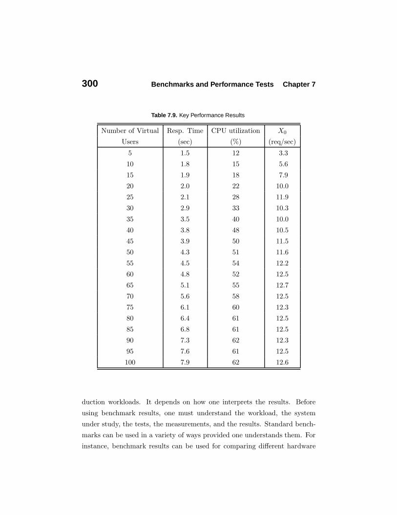
SUT and isolate the specific performance issue. Table 7.9 shows the response

time and CPU utilization measured for a varying number of virtual users.

At first glance, we observe that as new users are added to the system,

the response time increases. We also observe that the CPU utilization levels

off at 60%, which indicates the system has reached a bottleneck. Let us use

some simple models to understand the performance data. For each value of

N , the system can be represented by a closed model and we can use Little’s

Law to calculate the system throughput X0 = N/R. So, dividing the first

column by the second one of Table 7.9, we get the throughput, that is shown

in the fourth column of the same table. We also know that X0 = Ui/Di,

for each component i of the system. Considering that the maximum value

for Ui is 100%, we have that X0 ≤ 1/Di. The maximum system throughput

observed is around 12.5 and indicates that some component of the system,

rather than the CPU, has reached 100% utilization and is limiting the system

throughput. Because the response time has exceeded the limit of 2 seconds,

the main recommendation at this point is to get the application vendor

involved in the testing process to find out the origins of the performance

bottleneck.

7.7 Concluding Remarks

This chapter presented several industry standard benchmarks. They provide

a standard yardstick for comparing performance across different systems.

As pointed out in the introduction, benchmark results can both inform and

confuse users about the real capacity of systems to execute their actual pro-


Table 7.9. Key Performance Results

Number of Virtual Resp. Time CPU utilization X0

Users (sec) (%) (req/sec)

5 1.5 12 3.3

10 1.8 15 5.6

15 1.9 18 7.9

20 2.0 22 10.0

25 2.1 28 11.9

30 2.9 33 10.3

35 3.5 40 10.0

40 3.8 48 10.5

45 3.9 50 11.5

50 4.3 51 11.6

55 4.5 54 12.2

60 4.8 52 12.5

65 5.1 55 12.7

70 5.6 58 12.5

75 6.1 60 12.3

80 6.4 61 12.5

85 6.8 61 12.5

90 7.3 62 12.3

95 7.6 61 12.5

100 7.9 62 12.6

duction workloads. It depends on how one interprets the results. Before

using benchmark results, one must understand the workload, the system

under study, the tests, the measurements, and the results. Standard bench-

marks can be used in a variety of ways provided one understands them. For

instance, benchmark results can be used for comparing different hardware


systems running the same software or different software products on one

system. They can also be used to compare different models of systems in

a compatible family. Standard benchmarks, though, are not adequate tools

for capacity planning for a system with a customized workload. However,

benchmark results can be used in conjunction with performance models for

capacity planning purposes.

This chapter also examined performance testing issues. Performance

testing is a commonly used method to determine how users will experience

the performance of a Web service. The main purpose of running perfor-

mance tests is to understand the performance of the service under specific

workload conditions. Here we define a performance testing methodology

based on the use of automatic load testing tools. As we saw in the vari-

ous examples of this chapter, benchmark results can provide useful input

information for performance models. Also, simple analytic models can help

in the understanding of the meaning of results provided by benchmarking

and performance testing. Next chapters show how to construct performance

model of Web services.

Bibliography

[1] V. A. F. Almeida, M. Crovella, A. Bestavros, and A. Oliveira, “Char-

acterizing Reference Locality in the WWW,” Proc. IEEE/ACM Interna-

tional Conference on Parallel and Distributed System (PDIS), Miami Beach,

Florida, Dec. 1996, pp. 92–103.

[2] M. Arlitt and C. Williamson, “Web Server Workload Characterization:

The Search for Invariants,” Proc. 1996 ACM SIGMETRICS Conf. Mea-

surement Comput. Syst., ACM, Philadelphia, Pennsylvania, May 1996, pp.

126–137.

[3] P. Barford and M. Crovella, “Generating Representative Web Workloads

for Network and Server Performance Evaluation,” Proc. 1998 ACM SIG-


METRICS Int. Conf. Measurement and Modeling of Computer Systems,

Madison, Wisconsin, June 22-26, 1998, pp. 151–160.

[4] J. Gray, ed., The Benchmark Handbook for Database and Transaction

Processing Systems , 2nd ed., Morgan Kaufmann, San Mateo, California,

1993.

[5] J. Hennessy and D. Patterson, Computer Architecture: A Quantitative

Approach, Morgan Kaufmann, San Francisco, California, 1996.

[6] J. Henning, “SPEC CPU2000: Measuring CPU Performance in the New

Millennium,” Computer , IEEE, July 2000.

[7] U. Krishnaswamy and I. Scherson, “A Framework for Computer Perfor-

mance Evaluation Using Benchmark Sets,” IEEE Trans. Computers, vol. 49,

no. 12, Dec. 2000.

[8] D. Lilja, Measuring Computer Performance, Cambridge University Press,

Cambridge, United Kingdom, 2000.

[9] D. A. Menasce, V. A. F. Almeida, and L. W. Dowdy, Capacity Planning

and Performance Modeling: From Mainframes to Client-Server Systems ,

Prentice Hall, Upper Saddle River, New Jersey, 1994.

[10] D. Lipshultz, “Letting the World Plug into Your PC, for a Profit,” The

New York Times, June 3, 2001.

[11] System Performance Evaluation Corporation, www.spec.org

[12] J. Shaw, “Web Application Performance Testing - a Case Study of an

On-line Learning Application,” BT Technology Journal , vol. 18, no. 2, April

2000.

[13] M. Schwartz, “Test Case,” Computerworld, Aug. 14, 2000.

[14] G. Trent and M. Sake, “WebSTONE: the First Generation in HTTP

Benchmarking, MTS Silicon Graphics , Feb. 1995.


[15] Transaction Processing Performance Council, www.tpc.org

[16] N. Yeager and R. McCrath, Web Server Technology , Morgan Kaufmann,

San Francisco, California, 1996.

benchmarks and performance tests - pearson...

Documents