University of Massachusetts AmherstScholarWorks@UMass Amherst

Masters Theses 1911 - February 2014

2012

Benchmarking Virtual Network MappingAlgorithmsJin ZhuUniversity of Massachusetts Amherst

Follow this and additional works at: https://scholarworks.umass.edu/theses

Part of the Systems and Communications Commons

This thesis is brought to you for free and open access by ScholarWorks@UMass Amherst. It has been accepted for inclusion in Masters Theses 1911 -February 2014 by an authorized administrator of ScholarWorks@UMass Amherst. For more information, please contactscholarworks@library.umass.edu.

Zhu, Jin, "Benchmarking Virtual Network Mapping Algorithms" (2012). Masters Theses 1911 - February 2014. 970.Retrieved from https://scholarworks.umass.edu/theses/970

VNMBENCH: A BENCHMARK FOR VIRTUAL NETWORK MAPPING ALGORITHMS

A Thesis Presented

by

JIN ZHU Submitted to the Graduate School of the

University of Massachusetts Amherst in partial fulfillment of the requirements for the degree of

MASTER OF SCIENCE IN ELECTRICAL AND COMPUTER ENGINEERING

September 2012

Electrical and Computer Engineering

VNMBENCH: A BENCHMARK FOR VIRTUAL NETWORK MAPPING ALGORITHMS

A Thesis Presented

by

JIN ZHU Approved as to style and content by: Tilman Wolf, Chair

Weibo Gong, Member

Aura Ganz, Member C.V.Hollot, Department Head Electrical and Computer Engineering

ABSTRACT VNMBENCH: A BENCHMARK FOR VIRTUAL NETWORK MAPPING

ALGORITHMS

September 2012

Jin Zhu

B.E, NANJING UNIVERSITY OF POSTS AND TELECOMMUNICATIONS

M.S, UNIVERSITY OF MASSACHUSETTS AMHERST

Directed by: Professor Tilman Wolf

The network architecture of the current Internet cannot accommodate the

deployment of novel network-layer protocols. To address this fundamental problem,

network virtualization has been proposed, where a single physical infrastructure is

shared among different virtual network slices. A key operational problem in network

virtualization is the need to allocate physical node and link resources to virtual

network requests. While several different virtual network mapping algorithms have

been proposed in literature, it is difficult to compare their performance due to

differences in the evaluation methods used. In this thesis work, we proposed

VNMBench, a virtual network mapping benchmark that provides a set of standardized

inputs and evaluation metrics. Using this benchmark, different algorithms can be

evaluated and compared objectively. The benchmark model separate into two parts:

static model and dynamic model, which operated in fixed and changed mapping

process. We present such an evaluation using three existing virtual network mapping

algorithms. We compare the evaluation results of our synthetic benchmark with those

of actual Emulab requests to show that VNMBench is sufficiently realistic. We

believe this work provides an important foundation to quantitatively evaluating the

performance of a critical component in the operation of virtual networks.

iii

ACKNOWLEDGEMENT

First and foremost, I would like to express the deepest appreciation to my advisor,

Professor Tilman Wolf, who has the attitude and the substance of a genius and who

inspired my interest in computer networking. Without his guidance and persistent help

this thesis project would not have been possible. He always encourages me and inspires

me with lots of valuable and insights ideas.

I would like to thank my committee members, Professor Weibo Gong, and

Professor Aura Ganz, for their constructive advice and invaluable help on both of my

research and future career.

I also would like to acknowledge the members in the Network Systems Lab for the

knowledge and experience they have shared with me. In particular, I want to thank

Cong Wang, Shashank Shanbhag and Arun Kumar Kandoor, who helped me a lot on

this great project.

In additional, I would like to convey thanks to the Intel for providing the

laboratory facilities.

Finally, I appreciate all of the sincere support from my family and my friends, this

thesis pales in comparison to what I gained from them.

iv

TABLE OF CONTENTS

Page ABSTRACT ..................................................................................................................... iii ACKNOWLEDGEMENT ................................................................................................ iv LIST OF TABLES .......................................................................................................... viii LIST OF FIGURES .......................................................................................................... ix CHAPTER 1. INTRODUCTION ...................................................................................................... 1

1.1 Network Virtualization and Benchmark ............................................................... 1 1.2 Objectives ............................................................................................................ 3 1.3 Contributions ........................................................................................................ 4 1.4 Thesis Organization ............................................................................................. 5

2. RELATED WORK ..................................................................................................... 6

2.1 Network Virtualization System ............................................................................ 6 2.2 Current Models for Internet Structure .................................................................. 8 2.3 Current Exist Mapping Algorithms ...................................................................... 9

3. VNMBENCH ........................................................................................................... 12

3.1 Static VNMBench Model ................................................................................... 13

3.1.1 Operation of Benchmark ....................................................................... 13 3.1.2 Benchmark Inputs .................................................................................. 14

3.1.2.1 Topology Generation ............................................................. 14 3.1.2.2 Substrate Network ................................................................. 15 3.1.2.3 Virtual Network Requests ...................................................... 17 3.1.2.4 Parameter Settings ................................................................. 17

v

3.2 Dynamic VNMBench Model ............................................................................... 18

3.2.1 Operation of Benchmark ......................................................................... 18 3.2.2 Parameter Settings .................................................................................. 20

3.3 Related Methodology Conceptions ...................................................................... 22

3.3.1 Transit-Stub Topology Generator ............................................................ 22 3.3.2 Waxman Topology Generator ................................................................. 24 3.3.3 Little’s Law ............................................................................................ 25

4. VN MAPPING ALGORITHMS ................................................................................ 27

4.1 Existing Virtual Network Mapping Algorithms .................................................... 27

4.1.1 Rethinking Virtual Network Embedding: Substrate Support for Path Splitting and Migration[35] .................................................. 27

4.1.2 Virtual Network Embedding with Coordinated Node and Link Mapping[8] ....................................................................................... 29

4.1.3 A Virtual Network Mapping Algorithm based on Subgraph Isomorphism Detection[20] ............................................................... 31

4.2 Related Mathematical Conception ....................................................................... 34

4.2.1 Multi-commodity Flow problem ............................................................. 34 4.2.2 Subgraph Isomorphism Based Method .................................................... 36

5. EVALUATION RESULTS ........................................................................................ 37

5.1 Experiment Environment ..................................................................................... 37

5.1.1 Mapping Algorithm Implement ............................................................... 37 5.1.2 Network Generation ................................................................................ 38 5.1.3 Evaluation Metrics .................................................................................. 40

5.2 Static VNMBench Model .................................................................................... 44

5.2.1 Successful Mapping and Revenue-to-Cost Ratio ..................................... 44 5.2.2 Running time .......................................................................................... 50 5.2.3 Comparison of VNMBench Results and Emulab Results ......................... 52

5.3 Dynamic VNMBench Model ............................................................................... 55

5.3.1 Comparison of Successful Mapping Iteration .......................................... 56 5.3.2 Comparison of Different Average Amount of Active

Requests ........................................................................................... 65 5.3.3 Conclusion of Experiment Results ........................................................... 70

vi

6. CONCLUSION ...................................................................................................... 71 BIBLIOGRAPHY ....................................................................................................... 73

vii

LIST OF TABLES

Table Page

2.1 Parameters Comparison on Virtual Network Mapping Algorithms ....................... 11

3.1 Parameters of Substrate Network Topology Generator ......................................... 18

3.2 Parameters of Virtual Network Requests Topology Generator .............................. 18

3.3 Average Duration Time of Requests Setting in Different Situation ....................... 21

3.4 Parameters and Restriction of GT-ITM ................................................................ 24

4.1 Parameters of Evaluation Environment in the GMCF algorithm ........................... 29

4.2 Parameters of Evaluation Environment in the D-ViNE algorithm ......................... 31

4.3 Parameters of Evaluation Environment in the VnmFlib algorithm ........................ 34

5.1 Parameters setting in the Topology Generation .................................................... 39

5.2 Parameters Explanation in the Topology Generation ............................................ 39

viii

LIST OF FIGURES

Figure Page

1.1 The configuration of Virtual Network Mapping Problem ......................................... 3

3.1 The Virtual Network Requests Topology Examples .............................................. 17

3.2 LifeTime Distribution of Virtual Requests ............................................................. 21

3.3 The Transit-Stub Topology ................................................................................... 23

3.4 Number of items in a queuing system versus time .................................................. 26

5.1 Example of Revenue-To-Cost Computation .......................................................... 43

5.2 Comparison of Amount of Successful Mapping and Revenue-to-Cost Ratio(Dense Substrate Network with 100 Nodes) ............................................ 46

5.3 Comparison of Amount of Successful Mapping and Revenue-to-Cost

Ratio(Sparse Substrate Network with 100 Nodes) ........................................... 47

5.4 Comparison of Amount of Successful Mapping and Revenue-to-Cost Ratio(Dense Substrate Network with 500 Nodes) ............................................ 48

5.5 Comparison of Amount of Successful Mapping and Revenue-to-Cost

Ratio(Sparse Substrate Network with 500 Nodes) ........................................... 49

5.6 Comparison of Time and Number of Revenue-to-Cost Ratio (Substrate Network with 100 Nodes) .............................................................. 51

5.7 Comparison of Time and Number of Successful Mapping(Substrate

Network with 100 Nodes) .............................................................................. 51

5.8 Comparison of Time and Number of Successful Mapping(Substrate Network with 500 Nodes) .............................................................................. 52

5.9 Result Comparison between Emulab requests and VNMBench

(Sparse Substrate Network with 100 Nodes) .................................................... 54

ix

5.10 Result Comparison between Emulab requests and VNMBench (Dense Substrate Network with 100 Nodes ) ............................................................... 55

5.11 Comparison of Amount of Successful Mapping in Different Amount of

active requests (Dense Substrate Network with 100 Nodes, Virtual Network with 5 Nodes) ................................................................................. 58

5.12 Comparison of Amount of Successful Mapping in Different Average

Duration Time (Dense Substrate Network with 100 Nodes, Virtual Network with 10 Nodes) ................................................................... 59

5.13 Comparison of Amount of Successful Mapping in Different Average

Duration Time (Dense Substrate Network with 100 Nodes, Virtual Network with 20 Nodes) ................................................................... 60

5.14 Comparison of Amount of Successful Mapping in Different Average

Duration Time (Sparse Substrate Network with 100 Nodes, Virtual Network with 5 Nodes) ..................................................................... 61

5.15 Comparison of Amount of Successful Mapping in Different Average

Duration Time (Sparse Substrate Network with 100 Nodes, Virtual Network with 10 Nodes) ................................................................... 62

5.16 Comparison of Amount of Successful Mapping in Different Average

Duration Time (Dense Substrate Network with 500 Nodes, Virtual Network with 5 Nodes) ..................................................................... 63

5.17 Comparison of Amount of Successful Mapping in Different Average

Duration Time (Sparse Substrate Network with 500 Nodes, Virtual Network with 5 Nodes) ..................................................................... 64

5.18 Comparison of Different Average Amount of Active Requests (Dense

Substrate Network with 100 Nodes, Virtual Network with 5 Nodes) ........................................................................................................... 65

5.19 Comparison of Different Average Amount of Active Requests (Dense

Substrate Network with 100 Nodes, Virtual Network with 10 Nodes) ........................................................................................................... 66

5.20 Comparison of Different Average Amount of Active Requests (Dense

Substrate Network with 100 Nodes, Virtual Network with 20 Nodes) ........................................................................................................... 67

x

5.21 Comparison of Different Average Amount of Active Requests (Sparse Substrate Network with 100 Nodes, Virtual Network with 5

Nodes) ........................................................................................................... 68

5.22 Comparison of Different Average Amount of Active Requests (Sparse Substrate Network with 100 Nodes, Virtual Network with 10

Nodes) ........................................................................................................... 69 xi

CHAPTER 1

INTRODUCTION

1.1 Network Virtualization and Benchmark

As the Internet has grown to a global communication infrastructure that con-

nects large numbers of diverse distributed applications, new requirements for func-

tionality and performance have emerged. These requirements include security (e.g.,

protection against address spoofing), diverse communication paradigms (e.g., content-

addressable networks), and quality of service (e.g., performance guarantees for stream-

ing media).

The current Internet architecture cannot accommodate these requirements since

the Internet Protocol (IP), which is used by all systems in the Internet, cannot be

changed without creating incompatibilities [10]. While some shortcomings of IP can

be addressed by middle-boxes [16], such as firewalls [22] or network address translators

[13], they do not provide a general solution that can adapt to fundamentally different

network layer protocols, such as content-addressable networking [17].

An alternative network architecture that provides fundamental flexibility in the

protocols that are deployed, including the network layer protocol, is network virtual-

ization [2], [27]. In network virtualization, a single physical infrastructure is shared

among multiple virtual network slices (similar to how operating system virtualization

allows multiple different operating systems to share a single computer). Network

virtualization supports multiple coexisting heterogeneous network architecture from

different service providers with independent applications or protocols, called Virtu-

al Networks (abbreviates as VN) sharing a common physical substrate managed by

1

multiple infrastructure providers, called Substrate Network (abbreviates as SN) [6].

Through decoupling service providers from infrastructure providers, network virtual-

ization introduces flexibility for innovation and change.

Figure 1.1 gives the model of virtual network mapping. In the SN (the gray net-

work in the Figure 1.1), nodes are representative of the basic network infrastructure,

such as routers and hosts, which are interconnected by physical links. VN (the red

network in the Figure 1.1) is a group of virtual nodes (such as virtual routers) that

are hosted on different substrate nodes and interconnected by dedicated virtual links

over a substrate network. Multiple virtual networks may share the same underlying

substrate network resources. The substrate nodes have distributed fixed resources

such as CPU and substrate links have bandwidth resources. Each VN request has

also resource constraints, such as processing resources on the nodes and bandwidth

resources on the links, sometimes we even consider the additional constraints such

as node location or link propagation delay. When there is a VN request needs to

process, the service providers are responsible to form the substrate network into a

slide, to satisfy the requests embedding.

A key challenge in operating virtual networks is the problem of assigning logical

nodes and links to physical resources. Specifically, mapping a new VN, with con-

straints on the virtual nodes and links, on to specific physical nodes and links in

the SN. This virtual network mapping problem has received considerable attention in

recent years [7, 14, 34, 40] because it is a NP hard multi-way separator problem[1],

even if all the VN requests are known in advance, and because improvements in the

quality of mapping algorithm can significantly improve how many virtual networks

can be accommodated in an infrastructure and reduce the consuming time.

Despite the attention focused on the virtual network mapping problem, it is still

difficult to judge how well different algorithms perform under realistic operational con-

ditions. Every proposed virtual network mapping algorithm has the specific metrics

2

Figure 1.1: The configuration of Virtual Network Mapping Problem

with SN and VN. Some performance settings use small size of SN (amount of nodes

around 50)with a high node degree(more than 10) [34]; some set the nodes restriction

of CPU and link restriction of bandwidth in VN, however others use distance-based

constraints instead [18]; some algorithms consider the different distribution of edges in

the VN and the effect of ”alive” time of VN requests in the requirement [25]. So how

to use a benchmark to fair judge the performance of diversity mapping algorithms

becomes a significant key in the network virtualization. Perhaps one algorithm may

perform better for a particular scenario, but might have much less success mappings

when there is a small change in the setting of environment.

1.2 Objectives

The primary objective of this thesis project is to provide a benchmark to make

a quantitative comparison between competing mapping algorithms. Important cri-

3

teria of this benchmark are that the inputs (i.e., the virtual network substrate and

the virtual network requests) are representative of what would be encountered in a

real virtual network system, and the selected metrics used to judge the algorithms

could representative of the mainly and important performance in the virtual network

mapping problems. In order to illustrate the benchmark is sufficiently realistic, it

also needs to compare the evaluation results of synthetic benchmark with the actual

requests.

1.3 Contributions

1. Design of a benchmark, VNMBench, for evaluating virtual network mapping

algorithms. The benchmark consists of a variety of substrate network configu-

rations and virtual network requests and of a set of evaluation metrics that are

meaningful in this context.

2. Discussion of the representativeness of VNMBench (i.e., why the specific inputs

used by the benchmark can be considered typical for a virtual network mapping

environment).

3. Evaluation of three existing virtual network mapping algorithms using VNM-

Bench. The results demonstrate the types of quantitative results that can be

obtained for determining the performance of any given virtual network mapping

algorithm.

4. Comparison of mapping results obtained from VNMBench with results obtained

from real network virtualization environment (i.e., Emulab[32]). The compari-

son results show that the synthetic VNMBench requests lead to similar mapping

results, thus showing that VNMBench generates a representative workload

4

5. Separate the VNMBench model into two kinds: static model and dynamic mod-

el. Evaluate the performance of different mapping algorithms in situation of

fixed virtual requests duration time and changed virtual requests duration time.

1.4 Thesis Organization

The remainder of thesis is organized as follows: Chapter 2 presents the back-

ground on network virtualization and the related work in the benchmark creation.

Chapter 3 introduces the VNMBench model in detail, separate into static model and

dynamic model, including the method of topology generation and classification of

substrate network and virtual network requests. The existing three main VN map-

ping algorithms are presented in the Chapter 4,we introduce the basic mathematical

conceptions and process of these algorithms. In Chapter 5, we present the evaluation

results by VNMBench to make a comparison between three mapping algorithms in

static VNMBench model and dynamic static VNMBench model. The conclusion of

our benchmark is showed in Chapter 6.

5

CHAPTER 2

RELATED WORK

In this chapter, we first introduce the general conception of the network virtu-

alization system, points out three mainly requirements for modern virtual network

system. The realistic and accurate of network model, which could representative of

the real network, play a significant role on the research of many domains. From the

pure random methods to the hierarchical methods, researchers aim at finding the best

model for the constantly changing network. Different mapping algorithms using di-

versity evaluate environment and metrics to illustrate the performance of the mapping

results. At last, we list some typical benchmark used in the existed algorithms.

2.1 Network Virtualization System

In this section, we provide an exposition of the diversified Internet concept, the

solution to address the problem of the network ossification and the challenges.

The Internet plays a significant role in global commerce, media and defense, which

also becomes a critical infrastructure in the wide range of applications. However, the

ever-expanding scope and scale usage of the Internet also make it suffer from the ad-

verse effects of inertia. On the one hand, the existence of multiple stakeholders with

conflicting goals and policies creates a barrier to the deployment of new, radically

different technology. On the other hand, the end-to-end design of IP requires coor-

dination and the holistic agreement to deploy changes. At the same time, Internet

Service Providers (ISPs) lack of incentive to change their fixed patterns and models

due to their predominant role in the Internet works. All these reasons make the In-

6

ternet architecture suffer from the ossification, it is difficult to support diversity types

of applications such as global video conferencing, telephony and broadcast television.

Without supporting the diversity application impose a significant barrier of Internet

to innovation.

Thus, new requirements for functionality and performance have emerged. Some

of the examples as follows:

1. Security: With the increasing importance of the Internet, the network security

also plays a dominant role in the technologically advanced word. Guarantee the

authenticity of data and messages, protect systems from network-based attacks

and address spoofing, prevent the attack of the viruses, hackers and electronic

fraud are the significant fundamental element to approve the normal operation

of the Internet.

2. Diverse Communication Paradigm: Such as the Content Addressable Network

(CAN)[23], which is a distributed infrastructure that provides hash table-like

functionality on Internet-like scales. It is a scalable peer-to-peer file distribu-

tion system used in small and large scale storage management, which could

considered as a end-system virtualization.

3. Quality Of Service (QoS): QoS describes the performance of the applications

or traffic in the Internet. It includes the service differentiation and perfor-

mance assurance. Performance assurance for the Internet application such as

streaming media mainly including the bandwidth, loss of packets, delay. Service

differentiation is mainly about the IP address, port number and protocol.

Thus, with the proposal of the virtualization, it opens the opportunity for the

evolution path to the future Internet by deploying the different architectures and

protocols over a shared physical infrastructure, also could extenuate the ossifying

forces of the current Internet and stimulate innovation. The concept of the multiple

7

co-existing networks is not the new technique, current Internet infrastructure has al-

ready supported or potential to support a basic form of the network virtualization in

some parts. Such as T-Mobile UK and 3UK share network sites [15], VLAN(Virtual

Local Area Network) and MPLS(Multipreprotocol Label switching) are all the exam-

ples of the exist virtualization inside the network. A virtual private network, known

as VPN, which could connect multiple distributed sites shared a common physical in-

frastructure, is a specific virtual networks. But it is restricted that all virtual networks

are based on the same technology and protocol stack. Today the network virtualiza-

tion make a further step to achieve the independent programmability of the virtual

networks and want to handle multi-provider scenarios and hide the specificities of the

network infrastructure.[3], not just an illusory isolation, as provided by VPNs.

2.2 Current Models for Internet Structure

After having a historical perspective of the network virtualization, the important

part of designing the benchmark is the usage of the network topology generators to

generate realistic topologies. There are many examples to illustrate the significant

of the network model. Doar et al.[12] use the hierarchically structure graphs will

decrease around twice of inefficiency in their dynamic multicasting algorithms than

use the random graphs. Wei et al.[31] the traffic concentration is around 30% lower

in the shortest-path trees than the core-based trees., so the multiscale structure of

the Internet is fundamental to many network research problems.

But with the enormous smaller networks with potentially relevant distinctive prop-

erties and shortage of the shared topology information of network owners and oper-

ators, it is impossible to have a direct inspection of the network, and assess the

characterize and essential of network structure. Different empirical and theoretic ap-

proaches have developed by experimentalists and researchers. There are also many

8

methods to exploit phenomenological and graph-theoretic descriptions of large-scale

network structure and evaluate the ability of synthetic topology generators [4], [33].

The fundamental and popular topology generator to be used in the network sim-

ulation was the Waxman model [28], after inspecting into the real networks, we could

find that they are clearly not random but do exhibit certain obvious hierarchical

features. One of the standard topology generator is the Georgia Tech Internetwork

Topology Models(GT-ITM). A key point of the network connectivity should be con-

siderable attention is the heavy-tailed distributions in the node degree. In our work,

we choose to use GT-ITM tool to generate the substrate network and virtual network

requests.

2.3 Current Exist Mapping Algorithms

There are many mapping algorithms proposed to solve the virtual network map-

ping problem. Make efficient use of the substrate network, take the least time, increase

the amount of successful mapping are primary objectives of the mapping algorithms.

However, some challenges still exist for the mapping problem: First, node and link

constraints, which include the processing resources on the nodes, bandwidth resources

on the links, node location and link delay. Second, online requests, to be practical,

the arrival of virtual requests are based on a distribution rather than arrive at once

in a large collection. In additional, the duration time of requests are infinite, so the

mapped requests will stay in the substrate network all the time, or the duration time

of requests are limited, so they will be removed from substrate network when dura-

tion time expired. Third, the diverse topologies of the network, how to simulate a

real network topology and what kind of method to be used are key points in this

challenge.

A survey of network virtualization and virtual network mapping algorithms is

given in [6]. Some algorithms assume that the substrate network resources are un-

9

limited and restrict to allocating topologies to the substrate network, such as Fan

and Ammar [14]. To propose a solution for determining dynamic topology recon-

figuration, Zhu et al. [40] calculate the whole mapping periodically. Lu et al. [18]

make a termination constraints, distance constraints and pairwise traffic constraints

for the link and ignore the node constraints. It only uses a backbone star topology

for the offline requests process. Yu et al. [34] (GMCF) consider to use the general

and spoke topology as well as tree topology for the network model. They propose the

greedy heuristic for node mapping and multicommodity flow algorithm for the link

mapping, also process the online requests. Chowdhury et al.[8] (Dvine) supports the

path splitting and consider the online requests. The algorithm are separated into two

stages, and also uses the multicommodity flow algorithm for solving the link mapping

problem and integer program for the node mapping. Lischka et al.[20] combine the

two stages into one stage, and use the backtracking algorithm to solve the subgraph

isomorphism problem. The details of the algorithms GMCF, Dvine and VnmFlib

will be introduced in Chapter 4. The following table 2.1 lists the conditions and

parameters of different mapping algorithms.

Comparing evaluation results between published results is difficult because differ-

ent evaluation environments are used. Yu et al. [34] use a substrate network with

100 nodes and 500 links in a 100×100 grid, virtual network requests nodes with u-

niform distribution between 2 and 10, and CPU and link data rates with uniform

distribution between 0 to 100 units. However, Chowdhury et al. [8] use a 50-node

substrate network in a 25×25 grid, CPU requirements uniformly distributed from 0

to 20, and bandwidth resources uniformly distributed between 50 and 100. These

differences affect the results since parameters settings have an important effect on

the mapping result. Some mapping algorithms are more suitable for small networks

with a high node degree, some algorithms have a better performance in large and

sparse networks. The benchmark we develop in this paper can help in providing the

10

basis for fair and effective comparison of algorithms and to evaluate the advantages

and disadvantages of different approaches.

Table 2.1: Parameters Comparison on Virtual Network Mapping Algorithms

Mapping Link Nodes Online Request Optimizat-Algorithm Method Constraints Constr- Process Specifica- -ion Objec-

-aints -tion -tiveZhu et al. greedy; general achieve low[40] heuristic bandwidth CPU online topology & balanced

loadLu et al. integer termination; backbone average[18] program pairwise; tra- none offline star cost

-ffic distance topologyYu et al. greedy bandwidth CPU hub-spoke[34] heuristic; propagation location online tree revenue(GMCF) MCF delayChowdh- MCF; general average ac--ury et al. integer bandwidth CPU online topology -ceptance[8](Dvine) program location ratio; provi-

-sion cost;Lischka back- general revenue;[20] -tracking bandwidth CPU online topology cost load;(VnmFlib) balancing

11

CHAPTER 3

VNMBENCH

The benchmark we develop in the work consists of two components: (1) input sets

for virtual network mapping algorithms and (2) metrics for evaluating the outputs

of virtual network mapping algorithms. The inputs consist of a variety of different

scenarios that cover typical virtual network mapping uses. The metrics evaluate the

performance of virtual network mapping results in terms of the quality of the mapping

that was achieved and the running time. The following describes the general operation

of the benchmark, the various input parameter settings and metrics.

The benchmark provides parameters for generating two types of inputs: (1) one

substrate network, which represents the physical infrastructure on which virtual net-

works are mapped, and (2) multiple virtual network requests, which need to be

mapped onto the substrate network. Both links and nodes have constraints asso-

ciated with them. Substrate links provide a limited amount of bandwidth; substrate

nodes provide a limited amount of processing. Requests nodes are constrained in their

location and require processing resources. Paths between mapped request nodes re-

quire network bandwidth [35]. The mapping algorithms determine the placement of

request nodes and paths while avoiding resource conflicts in the substrate.

When multiple requests need to be mapped to a substrate, there are several differ-

ent ways of handling mapping operation: multiple requests could be mapped one after

another or at the same time; in case of incremental mappings, prior mappings can

be considered fixed or can be changed (e.g., in order to make scarce resources avail-

able to later mapping requests); once multiple mappings have completed, additional

12

mappings can be performed either until the substrate is full or prior mappings can

be removed as they expire. Clearly, these differences in operation have a considerable

impact on the results obtained from an evaluation of mapping algorithms.

In our work, we separate the VNMBench model into two kinds: static VNMBench

model and dynamic VNMBench model. The virtual network requests are fixed and

will occupy the substrate network resource permanently after successful mapping in

the static model. In the dynamic model, every request has a lifetime and will remove

from the substrate network when lifetime expired. We will introduce the topology

generation, parameter settings of each model in this chapter.

3.1 Static VNMBench Model

3.1.1 Operation of Benchmark

In the static model, we aim to stress-test the algorithms under considerations.

Therefore, we choose (what we call online) operation, where virtual network requests

are mapped successively onto a substrate without ever removing (or changing) a

mapping that has been completed. With every successful mapping of a virtual network

request, the remaining substrate resources become increasingly sparse. Therefore,

finding mapping solutions becomes increasingly difficult. In case a virtual network

request cannot be accommodated, it is considered a failed mapping attempt and

the next virtual network request is processed. The mapping process continues for a

specified number of requests (in our case 1000). After all virtual network requests have

been processed, the number of successful mappings and other metrics are determined.

It is important to note that VNMBench can be used for any type of operation

since the input sets and (to some extend) the metrics are agnostic of the specific

operation. Thus, VNMBench users can adapt the benchmark for their specific use.

In the next section, we will introduce the Dynamic VNMBench Model.

13

3.1.2 Benchmark Inputs

In both static and dynamic VNMBench model, the inputs for the virtual network

mapping algorithm are a substrate network and multiple virtual network requests.

We model the substrate network as a weighted undirected graph denoted by GS =

(NS, ES), where NS is the set of the substrate nodes and ES is the set of the substrate

links. Each substrate node nSi ∈ NS has an associated processing capacity denoted

by c(nSi ). Each substrate link eSi (u, v) ∈ ESbetween two substrate nodes u and v is

associated with the bandwidth capacity value b(eSi (u, v)). We set λ(u, v) denote the

length of eSi (u, v) between two substrate nodes u and v.

A virtual network request is defined by a weighted undirected graphGV = (NV , EV ),

where NV is the set of the virtual nodes and EV is the set of the virtual links. The

processing resource requested by a virtual network node nVi ∈ NV is denoted by c(nV

i ),

for each virtual link eVi (u, v) ∈ EV also has the bandwidth capacity b(eVi (u, v)) .

The virtual network requests are divided into three sizes: small requests have

5 nodes, medium requests have 10 nodes, and large requests have 20 nodes. The

processing resources of all requests are uniformly distributed (between 0 and 20) and

link bandwidth requests are also uniformly distributed (between 0 and 30). A total

of 1,000 virtual network requests is generated for each run of the benchmark.

3.1.2.1 Topology Generation

Due to the explosive growth and diversity changing of networking, networks are

difficult to be modeled by a simple graph. A key challenge in VNMBench is to

determine how to generate representative topologies for the network substrate and

the virtual network requests. In general, networks are difficult to model. The standard

approach is to generate the a graph such that the key metrics match with those of

typical networks. There are mainly three kinds of methods to generate the graph,

flat random topologies, regular topologies, and hierarchical topologies.

14

The flat random method connects the set of nodes with a specific probability by

edges. It can control the number of edges of the graph by changing the probability of

connection of random nodes, but cannot control the configuration of the edges. It is

more suitable to generate small graphs because it may have high node degree when

generating large graphs [39], which is not typical for the Internet. Since the Internet

can be viewed as a collection of interconnected routing domains [9], the Trans-Stub

method generate large graphs efficiently with a realistic average node degree [39].

Therefore, we choose this method to generate our substrate network. For the edge

method, we use the improved Waxman method [21] (rather than the pure random

method or exponential method, which are more likely to have long edges).

To generate substrate and request topologies in VNMBench, we use the GT-ITM

tool [38]. For the substrate network, we use the Trans-Stub topology generation

method [39] and for virtual network requests, we use the Waxman method.

3.1.2.2 Substrate Network

In VNMBench, a topology generator that uses certain settings generates substrate

network and virtual request topologies randomly. To provide some control over the

topology, we fix the topology and size of the substrate network and the corresponding

processing resources and link bandwidth. To explore a range of network configura-

tions, we consider two substrate network sizes: medium size with 100 nodes and large

size with 500 nodes. Each substrate size is further separated by the distinction of link

density: dense substrate network has approximated two times the number of links of

the sparse substrate network.

We choose to use two different sizes of the substrate network in our benchmark

because real networks there are medium size networks (e.g., corporate or campus

network) and large size networks (e.g., national network). We set the two sizes to differ

by a factor of 5 in the number nodes. In VNMBench, the medium substrate networks

15

number of nodes is 100 and node placement is random within a (100×100) grid. In

the large substrate network, there are 500 nodes and placed within a (200×200) grid.

The density of the links in the network plays an important role in the virtual

network requests mapping, because it is easier for mapping algorithms to find suitable

substrate nodes and links in the dense style, but more difficult to solve the mapping

problems when the network is sparse. In VNMBench, the sparse substrate network

has 129 links and the dense substrate network has 255 links in the medium size, and

639 links and 1294 links, respectively, in the large size.

In order to create a realistic network, we fix the node degree of sparse substrate

network around 2.5 and dense substrate network around 5.1, which are close to the

realistic average node degrees 6 [39]. When the node number is 100 in sparse style,

the graph has 2 transit domains, each transit domain has an average of 2 nodes, 4

stub domains per transit node, and no extra transit-stub or stub-stub edges. Each

stub domain also has 6 nodes on average. According to the formula of the average

node degree of the transit stub graph, we can calculate the node degree of two kinds

substrate networks:

ND =2(Et + (1 + EsNs)K)

1 +KNs

(3.1)

where the Et and Es are the edge densities of the transit and stub domains, respec-

tively. Nsis the average nodes per stub domain, K is the average stub domains per

transit node. The average node degree is approximately 2.58. In the dense style, there

are 50 extra transit-stub links or stub-stub links and node degree is approximately

5.10.

The same as the large substrate network setting, the specific parameters as showed

in the table 3.1 .

16

3.1.2.3 Virtual Network Requests

We separate the Virtual Network Requests into three size, 5 nodes, 10 nodes and

20 nodes. generated by the Waxman method. In the Waxman model, the probability

of edges connected pairs of nodes u and v is based on the Euclidean distance between

them,

P (u, v) = αe−d(u,v)βL (3.2)

where d(u, v) is the distance from node u to node v, α > 0,β ≤ 1,Lis the maximum

distance between any two edges. Parameter α increases the number of edges in the

graph, and parameter β increases the ratio of long edges to short edges [29]. In our

benchmark, we set the α is in the range from 0.3 to 0.8 and β from 0.15 to 0.25.

Thus, for every virtual network request, the node degree is in the range of 2.5 to 5,

which is typical of actual network.

3.1.2.4 Parameter Settings

The VNMBench parameters are summarized Table 3.1 and 3.2. Figure 3.1 is the

examples of virtual network requests topology separately in 5 nodes, 10 nodes and 20

nodes.

Figure 3.1: The Virtual Network Requests Topology Examples

17

Table 3.1: Parameters of Substrate Network Topology Generator

Medium Size Large SizeSparse Dense Sparse Dense

Number of nodes 100 100 500 500Number of links 129 255 639 1294Node Degree 2.58 5.10 2.55 5.17Scale 100×100 100×100 200×200 200×200Transit domains 2 2 2 2Nodes per transit 2 2 5 5Stubs per transit node 4 4 7 7Nodes per sub 6 6 7 7Extra links 0 50 0 250

Table 3.2: Parameters of Virtual Network Requests Topology Generator

Small Medium LargeNumber of nodes 5 10 20Number of links [4,6] [9,15] [19,47]Edge method WaxmanProcessing Resource uniform distribution (0,20)Bandwidth Reaource uniform distribution (0,30)Range of α [0.3,0.8]Range of β [0.15,0.25]

3.2 Dynamic VNMBench Model

3.2.1 Operation of Benchmark

In the dynamic VNMBench model, we focus on the dynamic mapping capacity of

each algorithm. We also choose the online operation, the embedding algorithm must

handle VN requests as they arrive, rather than handling a large collection of requests

at once. However, the virtual network requests arrive dynamically and stay in the

substrate network for an arbitrary period of time before departing if they mapping

18

successfully. The model has many applications in the real life, such as a researcher

may start a new experiment at any time, to run for some duration based on the

needs of the experiment. Similarly, a service provider may deploy a new service at

any time, and continue supporting the service indefinitely, possibly discontinuing the

service when it is no longer profitable. If the users occupy the resources of substrate

network even through they don’t use them anymore, it will decrease the flexibility and

utilization of substrate network. Therefore, the substrate resources will be released

when the mapped virtual network requests expired the lifetime and departed, this

situation offer more opportunities and resources for the following virtual requests,

and also improve the utilization of substrate network resources.

The ”dynamic” mainly reflected in two respects in this model: one is the VN

requests arrival rate λ, the other is the duration time of VN requests in the substrate

network. In order to better compute the average amount of VN requests stayed in

the substrate network, we fix the requests arrival rate to 1/sec, and set the lifetime as

exponential distribution with average duration time N . According to the Little’s Law,

the long-term average number of requests in a stable system E is equal to the long-

term average effective arrival rate λ, multiplied by the average time a request spends

in the substrate network N ., which is entirely independent of any of the probability

distributions involved.

E = λ ·N (3.3)

In our work, we choose the different value of average duration time of VN requests

in each situation. When the average number of active VN requests in the substrate

network is small, most mapping algorithms could handle the arriving requests suc-

cessfully, so it is difficult to compare and evaluate the performance of them. With

the increasing of the average duration time of VN requests, the average amount of

active VN requests is rising. It is more difficult for algorithms to handle the VN

requests, so the divergence of performance in processing the VN requests and amount

19

of successful mappings will be more obvious in various algorithms. In additional, in

order to observe the algorithms performance in the steady state, we choose to use

the varied total number of requests rather than fixed 1000 in the static VNMBench

model. When the average duration time is only 50 unit time, every mapping algo-

rithm only needs to process 1000 requests, because the number of active VN requests

tend to in the steady stage around 50 after 300 mapping iteration. However, when

the average duration time is increasing to 1000 unit time, we need to set the total

number of mapping iteration as 5000.

3.2.2 Parameter Settings

The average duration time of requests settings are summarized in Table 3.3. We

choose different range for medium size network and large size network. From the ex-

periment results of static VNMBench model, we could find the larger size of substrate

network, the more VN requests could be mapped successfully. So we need to choose

the suitable amount of average number of requests in order to observe the variation

trend of different mapping algorithms.

We set the virtual requests arrival rate as 1/sec, and the duration time as the

exponential distribution with average number N . Figure 3.2 shows the cumulative

distribution function of typical average lifetime of requests.

20

Table 3.3: Average Duration Time of Requests Setting in Different Situation

SN:100 nodes SN: 500 nodesVN requests Sparse(link:129) Dense(link:255) Sparse(link:639) Dense(link:1294)

5 nodes

50, 100, 150 50, 100, 150 200, 300, 400 200, 300, 400200, 300, 350 200, 300, 400 500, 600, 700 500, 600, 700400, 450, 500 450, 500, 600 800, 900 800, 900600, 800, 1100 800, 900, 1100 1000, 1100 1000, 1100

10 nodes

50, 100, 150 50, 100, 200 50, 100, 200 50, 100, 200200, 250, 300 250, 300, 400 300, 400, 500 300, 400, 500400, 500 500, 600, 700 600, 700 600, 700700, 800 800, 1000 800, 900 800, 900

20 nodes5, 10, 20 50, 100, 150 100, 200 100, 20030, 40, 50 200, 250, 300 300, 400 300, 40060, 100 350, 450 500, 600 500, 600

0

0.2

0.4

0.6

0.8

1

0 1000 2000 3000 4000 5000

Cum

ulat

ive

Dis

trib

utio

n F

unct

ion

Average Lifetime of Request

Distribution of Request Lifetime

N300N500N800

N1100

Figure 3.2: LifeTime Distribution of Virtual Requests

21

3.3 Related Methodology Conceptions

3.3.1 Transit-Stub Topology Generator

There are mainly three kinds of the topology generation methods: the first is the

flat random graph method, which is a group of nodes distribute randomly in the plane

and add the edges probabilistically in these vertices, such as the Waxman method.

The second is the hierarchical method, which extends the topology based on the

original smaller network components. It mainly contains N-level method and transit-

stub method. The third is the degree-based method, which focus on generating the

network with the power-law degree distributions [5].

In our work, we choose to use the transit-stub topology method to model the real

word Internet topology. For the random graph method, it is insensitive to the edge

length between nodes and adds the edges in the topology without control for the

length. The random graph method prefer generating the longer edges, so leading to

the longer paths in terms of Euclidean distance and much higher node degree than the

realistic average amount. For the power-law degree distribution topology generation,

it mainly emphasis the degree and degree-rank exponents in the topology and solely

on how well the nodes degree distribution fit the real Internet topology [26]. It is

more suitable to resemble the large Internet scale. In our work, we generate the small

Internet topology with 20 nodes in the virtual network requests, 100 and 500 nodes

in the substrate network. So, we choose the transit-stub topology method to generate

the topology model.

The transit-stub topology method is one of the hierarchical methods of the network

topology generators, it contains two domains in the topology: transit domain and stub

domain [37]. The method to generate the model is as following: first, it generates a

connected stochastic graph as the transit domain, every node in the transit domain

representative of an entire transit domain. Then, for each node in the transit domain,

it is replaced by another connected random graphs representing the stub domains.

22

At last, add the additional edges interconnected between the transit domain and stub

domain or two stub domains. The Figure 3.3 is an example of transit-stub topology.

This method avoid the shortage of the high node degree appeared when the scale of

the Internet is increasing and could also control the detail edges connection in the

topology. In generating the topology, we could set the parameters in both the transit

domain and stub domain, including the average amount of the transit domain, the

average number of stub domains in transit node and the average number of nodes in

the stub domain.

Figure 3.3: The Transit-Stub Topology

In order to prove the desired locality characteristics: there are many constraints

related with the selected edges through restricting the weights of the edges. It prefers

choosing the intra-stub and intra-transit edges rather than any inter-stub and inter-

transit one; first choosing the all-transit path when there is the collision with any

path with three stubs; choose the direct connection between a pair of stub domains

in some specific situation. The details as following [36]:

23

Table 3.4: Parameters and Restriction of GT-ITM

Parameter MeaningWtt Weight of a transit-transit interdomain edgeWts Weight of a transit-stub interfdomain edgeWss Weight of a stub-stub interdomain edgeDtop Diameter of transit-domain connectivity graphDt Maximum diameter of any transit domain graphDs Maximum diameter of any stub domain graph

Wtt := ⌈Dt/2⌉ (3.4)

Wts := ⌈DtopWtt/2⌉+ ⌈(Dtop + 1)Dt⌉ (3.5)

Wss := Ds + 2Wts (3.6)

3.3.2 Waxman Topology Generator

Waxman method is put forward by Bernard M.Waxman, which is the common

network topology generator and widely used in model of the network problems. This

graph model aims at address the problem of multipoint connections in the packet

switched network.

The probability of the edges is mainly affected by Euclidean distance between the

nodes. After a set of nodes randomly distributed in a coordinate grid, each node is

assigned a fixed integer coordinates, the probability of the links connected any two

nodes is decided by

P (x, y) = αe−d(x,y)βL (3.7)

where d(x, y) is the distance from node x to node y, α > 0,β ≤ 1,L is the maximum

distance between any two edges. Parameter α increases the number of edges in the

graph, and parameter β increases the ratio of long edges to short edges [29].

24

There are also many other algorithms focus on the problem of routing multi-

cast connections in networks which are variations of the Waxman method, such as

Matthew et al.[21] and Liming et al.[30]. In order to ensure the average node degree

remains constant, without increasing with the number of nodes, Matthew et al.[21]

add another factor kε|ω| in the probability function, where ε is the average degree of

a node and |ω| is the amount of the nodes exist in the connected graph. Another

method is replacing the d(x, y) by a random number between 0 and L. In the GT-ITM

topology generator, call this method the Waxman2 model [36]

3.3.3 Little’s Law

The definition of Little’s Law is, under steady state conditions, the long-term

average number of items in a queuing system equals the long-term average effective

arrival rate multiplied by the average time that an item spends in the system [19].

E = λ ·N (3.8)

N= average waiting time in the system for an item

λ = average number of items arriving per unit time

E = average number of items in the queuing system

The relationship is remarkably simple and general. It implies that the item be-

havior is entirely independent of any of the probability distributions involved, and

hence requires no assumptions about the schedule according to which items arrive.

Figure 3.4 shows a realization of a queuing system, the y-axis is the n(t), the

number of items at time t in the queuing system, the x-axis is the time. In the time

period T, A(T ) is the cumulative number of items in the system, so the average queue

length L(T ) is L(T ) = A(T )/T , N(T ) is the cumulative number of arrivals, so the

average arrival rate during time period T is λ(T ) = N(T )/T , we could also calculate

the average waiting time in the system per arrival during T, define as W (T ) =

25

A(T )/N(T ). From the figure, we could find L(T ) and λ(T ) go up and down somewhat

as items arrive and later leave.

Figure 3.4: Number of items in a queuing system versus time

n(t) = the number of items in the queuing system at time t;

T = a long period of time;

A(T ) = the area under the curve n(t) over the time period T;

N(T ) = the number of arrivals in the time period T.

26

CHAPTER 4

VN MAPPING ALGORITHMS

In this chapter, we introduce three mapping algorithms GMCF, Dvine and Vnm-

Flib in details. GMCF algorithm has a contribution on presenting the path splitting

and path migration method in the mapping. Dvine algorithm combines the mixed in-

teger programming (MIP) formulation and multi-commodity flow algorithm, it points

out a new definition ”meta-nodes” and ”meta-edges” for the virtual requests to find

an optimal link in the most efficient way. For the VnmFlib algorithm, it combines the

links mapping stage and nodes mapping stage into one stage, and using the subgraph

isomorphism based method in solving the mapping problem. Then, we also present

the corresponding mathematical conception used in these algorithms.

4.1 Existing Virtual Network Mapping Algorithms

4.1.1 Rethinking Virtual Network Embedding: Substrate Support for

Path Splitting and Migration[35]

In order to mapping the virtual network requests to the substrate network as

much as possible, most algorithms focus on improving the effective of the heuristic

algorithm itself. At a different angle, this paper uses a new point at the improvement

of substrate network, the primary contribution as follows:

• The algorithm supports split the link request of the virtual network and map

to the substrate network with a flexible path-splitting ratio.

• The algorithm also supports that the existing successful virtual link requests

could be reoptimize periodically by the substrate network, select new idle links

27

or adapting the splitting ratios for the existing links, in order to better use the

substrate resources.

This algorithm based on two prerequisites: First, node and link constraints. The

paper considers the CPU capacity and location for the node restrictions and band-

width capacity for link restrictions. Second, the algorithm aims at resolve the online

problem, which is the virtual network requests are not known in advance and on the

contrary they arrive in the random time and stay in the network for an arbitrary

period of time before leaving. The paper points out the definition revenue and aims

at maximize the long-term average revenue as a objective of the embedding problem:

limT→∞

∑Tt=0R(Gv(t))

T(4.1)

where R(Gv(t)) is the virtual network requests at time t, including both the node

and link requirements.

The key point of the algorithm is the link splitting and link migration. The

algorithm uses the greedy node mapping algorithm, which maximize the substrate

resources to map the virtual nodes to the substrate nodes, so as to minimize the

usage of the resources at both the nodes and links [40]. After the node mapping,

the algorithm called the flexible link splitting, find the satisfied links in the substrate

network. In order to keep mapping successfully in the best performance, the algorithm

revisits the node mapping decisions for these virtual links. Here, the paper uses a

parameter Ttry to control the difference of the chosen links and parameter Tdur as a

threshold to choose the virtual requests for the link migrating, in order to exclude

the requests with short living time. The algorithm also uses the hash-based splitting

method to prevent the out-of-order packet delivery in the network, which could direct

all packets from the same flow to the same link.

28

But the algorithm also has some shortages. The algorithm only focused on the

path migration, without the node migration, which lean to the link successful map-

ping.

At last, the paper creates an evaluation environment to evaluate the performance

of the algorithm. The details of the parameters setting showed in the table 4.1.1.

In this paper, the evaluation of algorithm based on the online requests, the arrivals

of virtual network requests are in the Poisson process, the average amount of mean

requests is 5, the duration of the requests are based on exponential distribution with

average 10 time windows.

Table 4.1: Parameters of Evaluation Environment in the GMCF algorithm

Substrate Network Virtual Network Requests

NodesNumber:100

Amount Distribution:CPU distribution:Uniform [0,100] (units) Uniform [2,10]

EdgesNumber:500

Connected probability:0.5Bandwidth distribution:Uniform [0.100](units)

4.1.2 Virtual Network Embedding with Coordinated Node and Link Mapping[8]

This paper mainly focuses on the improvement of the coordination between the

nodes mapping phase and links mapping phase. It proposes two virtual network (VN)

algorithms D-ViNE (Deterministic VN Embedding) and R-ViNE (Randomized VN

Embedding), the former one use the deterministic rounding techniques and the later

one use the randomized rounding techniques on the solution of the linear program

in the mixed integer programming(MIP) formulation[24], which used to solve the

embedding problem. The main contribution of the paper as following:

29

• Introduce the new definition augmented substrate graph, meta-nodes and meta-

edges, which are supported to coordinate the two mapping phases. Augmented

substrate graph is the extension of the basic substrate network, contains the

clusters of substrate nodes and meta-nodes, meta-edges.

• Separate the algorithms into deterministic and randomized rounding techniques

to process the linear program. The paper relaxes the integer constraints in the

MIP due to the difficulty and infeasible of this problem, and uses these two

techniques to obtain the integer values and embed VN requests.

The paper also considers the nodes and link restrictions, uses the CPU capacity

weight, geographic location, and bandwidth capacity weight as prerequisites, the algo-

rithm also based on the online virtual network embedding problems. The objective of

the algorithm is to maximize the revenue and minimize the cost of the infrastructure

provider (InP) in a long time.

R(GV ) =∑

eV ∈EV

b(eV ) +∑

nv∈NV

c(nV ) (4.2)

C(GV ) =∑

eV ∈EV

∑eS∈ES

f eV

eS +∑

nV ∈NV

c(nV ) (4.3)

where b(eV ) denotes the bandwidth capacity weight of the virtual links, c(nV ) de-

notes the CPU capacity weight of the virtual nodes, f eV

eS denotes the total amount of

bandwidth allocated on the substrate link eS for virtual link eV .

Here, we mainly introduce the algorithm of D-ViNE, which is the algorithm esti-

mated in our benchmark. The algorithm first creates an augmented substrate graph,

then uses the augmentation method for the VN requests. The algorithm checks

whether the unmapped substrate nodes exist or not and satisfied for the specific VN

requests, if non-empty, the deterministic rounding procedure is initiated. D-ViNE

calculate a parameter pz for each substrate node in the corresponding cluster for each

30

virtual node, the cluster is divided according to the location of nodes in the substrate

network. pz is the product of the binary values of meta-edge and the total flow pass-

ing through the meta-edge in both directions. The algorithm maps the virtual node

onto the idle substrate node with the highest pz value. The higher the value, the

better the solution of the MIP is. Once the virtual nodes mapped successfully, the

algorithm use the multi-commodity flow algorithm [25] to map the virtual edges onto

the substrate links.

The detail of the evaluation environment in this paper is listed in the table. VN

requests also arrive in a Poisson process, the average rate is 4 in 100 time units and

the lifetime of each VN request is exponentially distributed with an average value

u = 1000 time units.

Table 4.2: Parameters of Evaluation Environment in the D-ViNE algorithm

Substrate Network Virtual Network Requests

NodesNumber:50 Amount Distribution:Uniform [2,10]CPU distribution: CPU distribution:Uniform [50,100] (units) Uniform [0,20] (units)

Edgesconnected probability: 0.5 Connected probability:0.5Bandwidth distribution: Bandwidth distribution:Uniform [50.100](units) Uniform [0,50](units)

4.1.3 A Virtual Network Mapping Algorithm based on Subgraph Isomor-

phism Detection[20]

Most of the Virtual Network Mapping(VNM) algorithms are separated into two

steps: the node mapping and the links mapping. This paper figures out a new map-

ping method: combine the two mapping stages into just one process. The evaluation

of the algorithm proves that this method could not only have better mappings but

also improve the running time of the process. The mainly contribution as follows:

31

• The paper use subgraph isomorphism based method in the Virtual Network

Mapping Problem(VNMP), integrate the two mapping stages into one mapping

process. After one node mapping successfully, the algorithm will check the

corresponding link mapping, until satisfy all the requirements of the nodes and

links.

• Set two parameters ε and ω, the former is the restriction of the length of sub-

strate paths which virtual links are mapped, the later is the restriction of the

number of mapping steps and force the algorithm to stop the search if the

amount of searching trend to enormous.

The paper set the CPU capacity with each node and data rate constraint with

each link and also add the error rate cost of each substrate link. Consider the online

mapping problems, the algorithm also consider the arrival time and the life time of

the Virtual Network Requests(VNR). For the node restriction, the constraint cost

function are defined by the sum of the cost function together

cost(M(GV )) =n∑

i=1

αi · costi(M(GV )) (4.4)

For the data rate or delay cost of the link, the constraint cost function is

costi(M(GV )) =∑l∈LV

CVi (l) · length(M(l)) (4.5)

VNMM(GV )denotes the virtual network mapping onto the substrate network, αidenotes

the tunable weight constant, for making a balance between different constraint costs.M(l)is

the substrate path mapped by the virtual link.

32

Let C1(n)denotes the CPU capacity of the node and C2(l)denotes the data rate

capacity of the link, so the cost function of each capacity is

cost1(M(GV )) =∑n∈NV

C1(n) (4.6)

cost2(M(GV )) =∑l∈LV

C2(l) · length(M(l)) (4.7)

where α1 and α2 are both equal to 1.

The algorithm use the R/C − Ratio(Revenue-to-Cost-Ratio) as the criterion of

algorithm performance.

R/C −Ratio =R(GV )

M(GV )(4.8)

R(GV ) = α1 ·∑n∈NV

C1(n) + α2 ·∑l∈LV

C2(l) (4.9)

The ratio set between 0 and 1, the larger of ratio, the better of the optimal mapping.

First, the algorithm use the genneigh() function to generate a set of node pairs

(nV , nP ), separately representative of the virtual nodes and substrate nodes, then add

the nodes to corresponding graph respectively. Second, use the valid() function to

check whether the resulting mapping from the first step is valid. If so, call the Vn-

mFlib algorithm, map the virtual links connected to the corresponding virtual nodes

into substrate network and check the data rate capacity of links as well, otherwise the

termination condition is checked. If it does not satisfy the termination condition, the

next node pair is examined. The genneigh() function have two effects, one is select

substrate nodes that satisfy the CPU constraint of the virtual nodes, the other one

is select the substrate links that within the link length restriction. The valid() func-

tion checks whether any node constraints are violated and whether there is broken

connections in the substrate network.

The detail of evaluation environment of the algorithm is list in the table, the

paper use the GT-ITM tool to generate the network topologies. Instead of setting the

33

specific number of the maximum amount of CPU and bandwidth capacity in virtual

network requests, the paper use β as the substitute number. The algorithm use the

Revenue-to-Cost ratio and running time as the metrics to evaluate the performance.

Table 4.3: Parameters of Evaluation Environment in the VnmFlib algorithm

Substrate Network Virtual Network Requests

NodesNumber:100 Amount Distribution:Uniform [2,10]CPU distribution: CPU distribution:Uniform [0,100] (units) Uniform [0,β] (units)

EdgesNumber:around 500 Connected probability:0.5Bandwidth distribution: Bandwidth distribution:Uniform [0.100](units) Uniform [0,β](units)

4.2 Related Mathematical Conception

In this section, we introduce two mathematical problems related to the mapping

algorithms, one is the Muti-commodity Flow Algorithm, the other is Subgraph Iso-

morphism Based Method. The former one mainly used in the link mapping stage of

GMCF and Dvine algorithms, the later one mainly used in the VnmFlib algorith-

m. Through understanding the key methods used in the algorithms, we could better

compare the difference and the similar of these algorithms.

4.2.1 Multi-commodity Flow problem

Multi-commodity flow problem is a network flow problem that allowing multi-

ple commodities between different sources and destination nodes to share the same

network. We suppose a directed graph G = (V,E), every edge (u, v) ∈ E has a

nonnegative capacity c(u, v) ≥ 0. There are k different commodities, defined as

K1, K2, ...Ki, ..., Kk, for ith commodity, we specify by Ki = (si, ti, di). Here, node si

34

is the source , node ti is the destination and di is the demand of the commodity Ki,

which is the capacity flow of the commodity i from the source to the destination.

Assume fi(u, v) is the flow of commodity i from the node u to node v, fuv =∑ki=1 fi(u, v) is the sum of the different commodity flows, so in order to satisfy the

link capacity constraints and flow conservation, the objective function is to minimize

the cost. For each commodity (u, v) ∈ V and each i = 1, 2, ...k, the total capacity of

links should less than the maximum nonnegative link capacity c(u, v):

k∑i=1

fi(u, v) ≤ c(u, v) (4.10)

fi(u, v) ≥ 0 (4.11)

For each capacity except the source and destination node, the incoming flow should be

equal to the outgoing flow, thus, for each i = 1, 2, ...k and for each u, v ∈ V − {si, ti}

∑v∈V

fi(u, v)−∑v∈V

fi(v, u) = 0 (4.12)

For the source and destination nodes, suppose the value of the flow is d units, so

∑v∈V

f(s, v)−∑v∈V

f(v, s) = d (4.13)

In addition to the capacity c(u, v) for each edge (u,v). we also suppose a real cost

a(u, v) for each edge. So if we send d units of flow from the source to destination

in one flow, we need to minimize the total cost C(u,v) of the flow, this problem is

defined as the minimum-cost-flow problem

C(u, v) =∑

(u,v)∈E

a(u, v)fi(u, v) (4.14)

35

4.2.2 Subgraph Isomorphism Based Method

Assume that there are two graphs, one is the original graph as Go = (N1, L1), the

other is a target graph as Gt = (N2, B2), the target of subgraph isomorphism problem

is to find a original graph in the target graph. if there exist a objective function

that prove the branch structure of the two graphs, it defined as isomorphism[11]. If

there exist an isomorphism between Gt and a subgraph of Go and M maps the part

of Go onto a part of Gt and vice versa, M is said to be a subgraph isomorphism.

For the vnmFlib algorithm, it extend the Vlib algorithm, which is also based on

Subgraph Isomorphism method. The mapping of links to paths which is shorter than

the predefined distance would also accepted.

36

CHAPTER 5

EVALUATION RESULTS

To demonstrate how VNMBench can be used in practice, we evaluate three map-

ping algorithms: GMCF [35], VnmFlib [20] and Dvine [8]. These algorithms are

typical representatives for virtual network mapping algorithms. Thus, showing that

VNMBench can be applied to all of them to provide comparative results illustrates

the usefulness of our virtual network mapping benchmark.

All algorithms are set to the best possible parameters as mentioned by the authors

and are presented with the input data generated by VNMBench. All algorithms can

use path-splitting and thus can map a virtual link onto multiple physical paths. A

virtual node can be mapped to any physical node in the substrate. The substrate

resources can be mapped at an arbitrarily fine granularity to virtual networks.

In this chapter, we first introduce the evaluation environment including the topol-

ogy generation, metrics and then point out the result of the comparison through the

VNMBench for three mapping algorithms. We separate the evaluation results into

two parts, one is based on the static VNMBench model and the other is based on

dynamic VNMBench model.

5.1 Experiment Environment

5.1.1 Mapping Algorithm Implement

In the Chapter 4, we have introduced the details and process of these three map-

ping algorithms. In order to better understand the result of the benchmark evaluation,

here we make a conclusion:

37

1. GMCF embedding algorithm: greedy node mapping algorithm and Multi-commodity

Flow Algorithm(MCF) link mapping algorithm.

2. D-ViNE embedding algorithm: deterministic rounding techniques on node map-

ping and MCF algorithm used in the link mapping

3. VnmFlib embedding algorithm: node and link mappings are both based on

subgraph isomorphism detection.

For the evaluation environment, GMCF and VnmFlib algorithm use almost the

same size and distribution in the substrate network and virtual network requests,

VnmFlib replace the fixed maximum value of CPU resources of virtual nodes into

variables. Dvine use a smaller size of substrate network and different CPU and band-

width distribution in nodes and links. In order to better evaluate the performance of

different mapping algorithms, we need to use the same evaluation criteria.

5.1.2 Network Generation

We use the GT-ITM to generate the substrate and virtual network topology. For

the substrate network, we separate the size of network into medium (100 nodes) and

large (500 nodes). For each size, we separate the density of network into sparse and

dense with different node degree. The details of parameters setting in the GT-ITM

file list in the table 5.1. For each parameter, the explanation is in the table 5.2.

First we choose one of the hierarchical models: transit-stub as the topology model,

and Waxman2 as the edge creation method, then set amount of stub domain and

transit domain. We add the extra transit-stub and stub-stub edges and increase the

probability of the connected edges in the dense substrate in order to increase the node

degree. The value of β set as 0.5 in all kinds of substrate networks in order to keep

the equal proportion of long edges and short edges.

38

Table 5.1: Parameters setting in the Topology Generation

Medium Size Large Size(A)Sparse (B) Dense (C) Sparse (D) Densets 1 100 ts 1 100 ts 1 100 ts 1 1004 0 0 4 50 50 7 0 0 7 250 2502 50 2 0.5 0.5 2 50 2 0.8 0.5 2 100 2 0.5 0.5 2 100 2 0.8 0.52 50 2 0.5 0.5 2 50 2 0.8 0.5 5 100 2 0.5 0.5 5 100 2 0.8 0.56 10 2 0.5 0.5 6 10 2 0.8 0.5 7 20 2 0.5 0.5 7 20 2 0.8 0.5

Table 5.2: Parameters Explanation in the Topology Generation

GT-ITM file Explanation

ts 1 100Graph Method:

Number of graphs Initial seedTransit-stub

4 0 0 Stub domain Extra transit-stub Extra stub-per transit node edges -stub edges

2 50 2 0.5 0.5 Top-level Transit One-sided dim-Waxman2 α β

parameter domain -ension of space2 50 2 0.5 0.5 Transit domain Nodes per One-sided dim-

Waxman2 α βparameter transit -ension of space

6 10 2 0.5 0.5 Stub domain Nodes per One-sided dim-Waxman2 α β

parameter stub -ension of space

39

The details of parameters in virtual network request is list in the table 3.2. Instead

of setting the fixed value of α and β, we use a random variable chosen in a range.

Thus, the node degree of each virtual network is in the range of 2.5 to 5, which could

also representative of the typical actual networks in sparse type and dense type.

5.1.3 Evaluation Metrics

In VNMBench, we consider three metrics to compare and evaluate mapping algo-

rithm performance: number of successful mapping, revenue-to-cost ratio, and running

time. In the Section IV, we compare three specific mapping algorithms with respect

to these metrics to show that meaningful inferences about algorithm performance are

possible.

1. Number of Successful Mappings

One of the main goals of the network virtualization is enable as much as pos-

sible multiple heterogeneous virtual networks to coexist together on a shared

substrate network. Even though each virtual network request has a different

topology, different processing resource on nodes and different bandwidth re-

source on links, the mapping algorithms should try to maximize the number

of the coexisting virtual network requests [6]. Therefore, we choose the total

number of successful mappings as one of the key metrics for VNMBench.

Note that this metric assumes online operation as discussed above. Also, it

is assumed that there are enough requests to completely fill up the substrate

network. In case a request cannot be mapped to the substrate, it is considered

a mapping failure. In this case, it can be distinguished if the mapping failed

due to the lack of node resources or link resources. This distinction may help

in understanding why the performance of a particular substrate network (or a

40

particular mapping algorithm) is limited. The virtual network mapping problem

requires the mapping algorithms to map virtual nodes and links in a given

request to substrate nodes and links. The successful mapping amount could be

separate into node successful mapping and link successful mapping, either one

is mapping failed would lead to this virtual network request denied. So we first

set the total successful mapping amount as a metric to evaluate the performance

of the different mapping algorithms.

2. Revenue-to-Cost Ratio

Another important metric is to measure the amount of substrate resources are

necessary to accommodate a request. In virtual network mapping, it is common

to refer to the complexity of a request as ”revenue” (i.e., how much customer

would pay for having their network installed in a substrate). The amount of

substrate resources necessary is referred to as ”cost” of a mapping.

We let the GVj = (NV

j , EVj ) denote the jth virtual network request, and define

the revenue, cost and the ratio of them with this request. The cost of mapping

the jth request is the total cost of allocation of substrate network resources to

the jth virtual network. We consider node resources and link resources, so the

total cost can be separated into two parts: the node mapping cost and the link

mapping cost.

We defined the total cost as

cost(GVj ) =

n∑i=1

αi · costi(GVj ) (5.1)

where αi is the weight constant for each cost to strike a balance between the

different constraint costs.

41

cost(GVj ) = α · costN(GV

j ) + β · costL(GVj ) (5.2)

We set the α as the node mapping cost factor, β as the link mapping cost

factor instead of α1 and α2, set the c(eVj ) as the demand of links in the jth

virtual network, λ(fE(u, v)) is the length of the path that the virtual link (u, v)is

mapped to the set of substrate links in GS. So the link mapping cost is

costL(GVj ) =

∑eVj (u,v)∈EV

j

λ(fE(u, v)) · c(eVj ) (5.3)

so the total mapping cost is defined as

C(GVj ) = α ·

∑nVj ∈NV

j

c(nVi )+

β ·∑

eVj (u,v)∈EVj

λ(fE(u, v)) · c(eVj )(5.4)

We define the Revenue R(GVj ) generated by the jth virtual network request as

R(GVj ) = α1 ·

∑nVj ∈NV

j

c(nVj ) + α2 ·

∑eVj (u,v)∈EV

j

c(eVj ) (5.5)

where α1 and α2 are weight constant for node and link revenue, we often set

α1 = α2 = 1.

The revenue-to-cost-ratio is based on the above definition:

R/C −Ratio =R(GV

j )

C(GVj )

(5.6)

the R/C − Ratio has values between 0 and 1. It is set to 0 when the virtual

network requests mapping fails and achieves 1 when an optimal virtual network

42

mapping is found, which means every virtual link uses a direct physical link in

the substrate.

In order to better understand the computation of revenue and cost, we make a

example to illustrate this evaluation metric in our work. The left part in the

Figure 5.1 is the virtual request and the right part is the substrate network.

After mapping the request into the substrate network (the blue dash network),

the revenues generated by virtual network is R = (12+14+16)+(10+8+6) = 66

(we set the α1 and α2 equal to 1) and the cost is C = (12+ 14+ 16) + (8× 1 +

10× 1 + 6× 2) = 72, so the ratio is 0.916.

Figure 5.1: Example of Revenue-To-Cost Computation

3. Running Time

The definition of running time is the average time of processing one virtual

network request by the mapping algorithm. The running time of a mapping

algorithms is of practical importance - especially since virtual network requests

are often handled dynamically in an online fashion. Therefore, the running time

of an algorithm is also a metric in our benchmark. We determine the average

time by measuring the total running time for all 1000 requests (including failed

mappings) and dividing accordingly.

43

5.2 Static VNMBench Model

In the static VNMBench Model, a total of 1000 requests are processed by each

algorithm. For solving the Dvine, GMCF and VnmFlib formulations, we have used

GLPSOL Optimization Studio. These experiments were run on Intel Quad-core CPU

running at 2.5 GHZ with 3 MB of level-2 cache and 3.4 G of main memory.

5.2.1 Successful Mapping and Revenue-to-Cost Ratio

Figure 5.2 and 5.3 show number of successful mappings and revenue-to-cost ratio

for sparse and dense substrate networks of medium size. Figure 5.4 and Figure 5.5

show the same metrics of large size in different density of network. The x-axis is the

request mapping iteration from 0 to 1,000 and the y-axis is the number of successful

mappings or the revenue-to-cost ratio up to that iteration. Each subgraph is shown

for virtual network requests of 5 nodes, 10 nodes, and 20 nodes.

For the medium substrate network, we can make the following observations from

Figure 5.2 and 5.3 :

• We find that the VnmFlib algorithm has the largest number of successful map-

pings and the highest revenue-to-cost ratio among all three algorithms in both

the sparse and dense substrate network. For dense substrate network, the suc-

cessful mappings of VnmFlib are approximately 3 times more than GMCF and

15 times than Dvine; For the sparse substrate network, the amount of success-

ful mappings of VnmFlib are around 4 times than GMCF and 22 times than

Dvine. The revenue-to-cost ratio is almost 1.5 times higher. All of the three

algorithms mapping requests successfully in the dense substrate than in the s-

parse substrate. Because the dense substrate network style has twice the node

degree of the sparse style, there are more possibilities to map edges successfully

for all algorithms.

44

• In both the sparse and dense substrate, GMCF can satisfy more virtual network

requests and has a higher revenue-to-cost ratio than Dvine. But, with an in-

creasing number of successful mappings, the revenue-to-cost ratio of Dvine and

VnmFlib also increase, but GMCF improves the number of successful mappings

at the expense of the revenue-to-cost ratio. In detail, we could find GMCF and

Dvine have the same failed node mapping amount, but Dvine has a higher failed

edge mapping amount than GMCF.

• Dvine is not good for large virtual network requests. When the size of virtual

request increase to 20 nodes, it could only map successfully 2 requests in the

dense substrate network.

For the large substrate network, we could find the following conclusion from Figure

5.4 and Figure 5.5:

• VnmFlib mapping requests successfully around 2 times than in the medium

substrate network, also has the most amount of successful mapping and the

highest revenue-to-cost ratio in the three algorithms.

• When the amount of virtual requests nodes increases to 10 and 20, mapping

of Dvine fails entirely, and only maps 17 requests with 5 nodes. So it is not

suitable for Dvine algorithm when the substrate networks and virtual network

requests in large size.

• With the increasing in the scale of virtual network requests, the difference be-

tween VnmFlib and GMCF in successful mappings and revenue-to-cost ratio

become smaller in dense network and become larger in sparse network.

Overall, for the medium and large size substrate network, the VnmFlib algorithm

is the best choice used, but it takes a lot of time (see below). If the emphasis is on

the amount of successful mapping, GMCF may be preferable. If the emphasis is on

revenue-to-cost ratio, then Dvine may be preferable.

45

0

20

40

60

80

100

0 200 400 600 800 1000No.

of S

ucce

ssfu

l Map

ping

s

Mapping Iteration

VN:5 nodes

0

10

20

30

40

50

0 200 400 600 800 1000No.

of S

ucce

ssfu

l Map

ping

s

Mapping Iteration

VN:10 nodes

0 2 4 6 8

10 12 14

0 200 400 600 800 1000No.

of S

ucce

ssfu

l Map

ping

s

Mapping Iteration

VN:20 nodes

0

0.2

0.4

0.6

0.8

1

0 200 400 600 800 1000

Rev

enue

-to-

cost

Rat

io

Mapping Iteration

VN:5 nodes

0

0.2

0.4

0.6

0.8

1

0 200 400 600 800 1000

Rev

enue

-to-

cost

Rat

io

Mapping Iteration

VN:10 nodes

0

0.2

0.4

0.6

0.8

1

0 200 400 600 800 1000

Rev

enue

-to-

cost

Rat

io

Mapping Iteration

VN:20 nodes

DvineGMCF

VnmFlib

Figure 5.2: Comparison of Amount of Successful Mapping and Revenue-to-CostRatio(Dense Substrate Network with 100 Nodes)

46

0

20

40

60

80

100

0 200 400 600 800 1000No.

of S

ucce

ssfu

l Map

ping

s

Mapping Iteration

VN:5 nodes

0

5

10

15

20

0 200 400 600 800 1000No.

of S

ucce

ssfu

l Map

ping

s

Mapping Iteration

VN:10 nodes

0 2 4 6 8

10 12 14

0 200 400 600 800 1000No.

of S

ucce

ssfu

l Map

ping

s

Mapping Iteration

VN:20 nodes

0

0.2

0.4

0.6

0.8

1

0 200 400 600 800 1000

Rev

enue

-to-

cost

Rat

io

Mapping Iteration

VN:5 nodes

0

0.2

0.4

0.6

0.8

1

0 200 400 600 800 1000

Rev

enue

-to-

cost

Rat

io

Mapping Iteration

VN:10 nodes

0

0.2

0.4

0.6

0.8

1

0 200 400 600 800 1000

Rev

enue

-to-

cost

Rat

io

Mapping Iteration

VN:20 nodes

DvineGMCF

VnmFlib

Figure 5.3: Comparison of Amount of Successful Mapping and Revenue-to-CostRatio(Sparse Substrate Network with 100 Nodes)

47

0

100

200

300

400

500

0 200 400 600 800 1000No.

of S

ucce

ssfu

l Map

ping

s

Mapping Iteration

VN:5 nodes

0

50

100

150

200

0 200 400 600 800 1000No.

of S

ucce

ssfu

l Map

ping

s

Mapping Iteration

VN:10 nodes

0 5

10 15 20 25 30 35 40

0 200 400 600 800 1000No.

of S

ucce

ssfu

l Map

ping

s

Mapping Iteration

VN:20 nodes

0

0.2

0.4

0.6

0.8

1

0 200 400 600 800 1000

Rev

enue

-to-

cost

Rat

io

Mapping Iteration

VN:5 nodes

DvineGMCF

VnmFlib

0

0.2

0.4

0.6

0.8

1

0 200 400 600 800 1000

Rev

enue

-to-

cost

Rat

io

Mapping Iteration

VN:10 nodes

0

0.2

0.4

0.6

0.8

1

0 200 400 600 800 1000

Rev

enue

-to-

cost

Rat

io

Mapping Iteration

VN:20 nodes

Figure 5.4: Comparison of Amount of Successful Mapping and Revenue-to-CostRatio(Dense Substrate Network with 500 Nodes)

48

0 50

100 150 200 250 300 350

0 200 400 600 800 1000No.

of S

ucce

ssfu

l Map

ping

s

Mapping Iteration

VN:5 nodes

0

10

20

30

40

50

0 200 400 600 800 1000No.

of S

ucce

ssfu

l Map

ping

s

Mapping Iteration

VN:10 nodes

0

2

4

6

8

10

0 200 400 600 800 1000No.

of S

ucce

ssfu

l Map

ping

s

Mapping Iteration

VN:20 nodes

0

0.2

0.4

0.6

0.8

1

0 200 400 600 800 1000

Rev

enue

-to-

cost

Rat

io

Mapping Iteration

VN:5 nodes

0

0.2

0.4

0.6

0.8

1

0 200 400 600 800 1000

Rev

enue

-to-

cost

Rat

io

Mapping Iteration

VN:10 nodes

0

0.2

0.4

0.6

0.8

1

0 200 400 600 800 1000

Rev

enue

-to-

cost

Rat

io

Mapping Iteration

VN:20 nodes

Figure 5.5: Comparison of Amount of Successful Mapping and Revenue-to-CostRatio(Sparse Substrate Network with 500 Nodes)

49

5.2.2 Running time

Figure 5.6 and Figure 5.7 show the distribution of number of successful mappings

and revenue-to-cost ratio with respect to the running time in the medium substrate

network. We observe that VnmFlib has the highest number of successful mappings

and revenue-to-cost ratio but also a longer running time. GMCF has the shortest

running time. Dvine performs the worst in the three mapping algorithms since it

takes more time than GMCF algorithm with a lower successful mapping amount.

Thus, one can choose to use the mapping algorithm with small running time

and corresponding higher successful mapping performance (such as GMCF) if one

emphasizes on the time to complete the mapping process. If one considers the amount

of successful mapping of virtual network requests as the only requirement, one can

choose the algorithm with the best performance in mapping (such as VnmFlib). In

addition, Dvine and VnmFlib are both a good choice if one aims to increase the

revenue-to-cost ratio with increasing successful mappings.

Figure 5.8 show the relationship of number of successful mapping with running

time in the large substrate network. Because Dvine has failed totally when the nodes

of virtual requests are 10 and 20, the graph mainly show the comparison of GMCF

and VnmFlib. From the graph, we could find the VnmFlib satisfy larger virtual

requests with a much longer running time than GMCF. Thus, for the large virtual

network mapping, we will choose GMCF if focus on the shorter running time and

choose VnmFlib if emphasis on the amount of successful mapping.

Clearly, the evaluation of these algorithms using static VNMBench model provides

interesting insights into the operation of and tradeoffs between algorithms. (We are

less focised on which particular algorithm outperforms another.)

50

0

0.2

0.4

0.6

0.8

1

0 20000 40000 60000 80000 100000

Rev

enue

to C

ost R

atio

Total Running Time (secs)

SN100:Time Vs Revenue-to-Cost Ratio

DvineGMCF

VnmFlib

Figure 5.6: Comparison of Time and Number of Revenue-to-Cost Ratio (SubstrateNetwork with 100 Nodes)

0

20

40

60

80

100

0 20000 40000 60000 80000 100000

Am

ount

of S

ucce

ssfu

l Map

ping

Total Running Time (secs)

SN100:Time Vs Amount of Successful Mapping

DvineGMCF

VnmFlib

Figure 5.7: Comparison of Time and Number of Successful Mapping(Substrate Net-work with 100 Nodes)

51

0

100

200

300

400

500

600

500000 1e+06 1.5e+06 2e+06 2.5e+06 3e+06 3.5e+06 4e+06

Am

ount

of S

ucce

ssfu

l Map

ping

Total Consuming Time (secs)

SN500:Time Vs Amount of Successful Mapping

DvineGMCF

VnmFlib

Figure 5.8: Comparison of Time and Number of Successful Mapping(Substrate Net-work with 500 Nodes)

5.2.3 Comparison of VNMBench Results and Emulab Results

A key requirement of any benchmark is that it generates a representative work-

load. To demonstrate that VNMBench generates a realistic set of virtual network

mapping requests, we compare these requests to requests that were issued by real

users in Emulab. Since it is difficult to compare the actual requests (due to topology,

parameters, etc.), we compare the mapping results obtained from both scenarios. If

the mapping results are similar in both cases, it can be assumed that the synthetic

requests issued by VNMBench are sufficiently representative of what happens in re-

ality in Emulab. (Of course, the benefit of a synthetic benchmark, like VNMBench,

is that it can be scaled to other configurations, which is not possible with traces.)

The Emulab request traces have topologies with 2 to 15 nodes. Since the traces do

not have explicit processing demands, we added them based on a uniform distribution

between 0 and 20. Edge bandwidth demands are uniformly distributed between 0

52

and 50. For comparison, we use the same substrate network generated in VNMBench

model with node processing resources and edge bandwidth resources set to 100 units

on a 100× 100 grid.

We separate the experiments into two parts. First, we extract 1000 requests with 5

nodes from the Emulab collected requests and make a comparison with 5-node virtual

network requests in VNMBench model. Figure 5.9 shows the number of successful

mappings and revenue-to-cost ratio of three mapping algorithms based on Emulab

requests and VNMBench requests in the sparse substrate network with 100 nodes.

From the figure, we observe the successful mapping amount of Dvine and GMCF are

equal in both scenarios and VnmFlib can successfully map 48 Emulab requests and

52 VNMBench requests. For the revenue-to-cost ratio, the value and variation trend

of the three mapping algorithms is also similar for Emulab requests and VNMBench

requests. For both scenarios, VnmFlib performs better than the other two algorithms

in these two metrics, GMCF has more successful mappings than Dvine, but with a

decrease of revenue-to-cost ratio. Thus, the results for VNMBench are extremely

similar to those for real Emulab requests.

When using Emulab requests with varying numbers of nodes, the comparison to

VNMBench becomes more difficult. Since we offer many topologies for mapping, the

algorithms will successfully map many of the smaller Emulab topologies. In contrast,

VNMBench uses the same size topologies and thus does not offer ”easy” mappings.

In the second part, we extract 1000 requests randomly from Emulab virtual network

requests and also using 5-node requests in VNMBench model to make a comparison

in the evaluation results of different mapping algorithms. The probability of node

number between 2 to 5 is around 0.6 in Emulab requests, the average node number

in the successful mapping requests is around 3 and average link number is around

2 when using GMCF and VnmFlib mapping algorithms. The smaller node and link

number, the easier for virtual network requests mapping successfully. Therefore,

53

the number of successful mappings is 118 for VnmFlib algorithm based on Emulab

requests, which is larger than the number of mappings from VNMBench requests.

For Dvine, the average node number of successful mapping is 4 and link number is 3,

which is similar to the VNMBench model (number of nodes is 5 and average number

of links is 4). Thus, Dvine has the same amount of successful mapping. Despite these

differences, there are still many similarities in the results, especially when considering

the revenue-to-cost ratio.

Thus, these comparisons show that VNMBench does generate inputs that are

representative of virtual network mapping requests generated in real virtualized net-

works.

0

20

40

60

80

100

0 200 400 600 800 1000

No.

of S

ucce

ssfu

l Map

ping

s

Mapping Iteration

Emulab VN Requests(5 nodes)

0

20

40

60

80

100

0 200 400 600 800 1000

No.

of S

ucce

ssfu

l Map

ping

s

Mapping Iteration

VNMBench VN Requests(5 nodes)

0

0.2

0.4

0.6

0.8

1

0 200 400 600 800 1000

Rev

enue

-to-

cost

Rat

io

Mapping Iteration

Emulab VN Requests(5 nodes)

DvineGMCF

VnmFlib 0

0.2

0.4

0.6

0.8

1

0 200 400 600 800 1000

Rev

enue

-to-

cost

Rat

io

Mapping Iteration

VNMBench VN Requests(5 nodes)

Figure 5.9: Result Comparison between Emulab requests and VNMBench (SparseSubstrate Network with 100 Nodes)

54

0

20

40

60

80

100

120

0 200 400 600 800 1000

No.

of S

ucce

ssfu

l Map

ping

s

Mapping Iteration

Emulab VN Requests

0

20

40

60

80

100

120

0 200 400 600 800 1000

No.

of S

ucce

ssfu

l Map

ping

s

Mapping Iteration

VNMBench VN Requests(5 nodes)

0

0.2

0.4

0.6

0.8

1

0 200 400 600 800 1000

Rev

enue

-to-

cost

Rat

io

Mapping Iteration

Emulab VN Requests

DvineGMCF

VnmFlib

0

0.2

0.4

0.6

0.8

1

0 200 400 600 800 1000R

even

ue-t

o-co

st R

atio

Mapping Iteration

VNMBench VN Requests(5 nodes)

Figure 5.10: Result Comparison between Emulab requests and VNMBench (DenseSubstrate Network with 100 Nodes )

5.3 Dynamic VNMBench Model

For the dynamic VNMBench Model, multiple virtual network requests are mapped

one after another with the arrival rate 1/sec, all requests have a limited duration

time, which means they will be removed from the substrate network and release

the corresponding nodes resources and link resources when the duration time expire

if they are mapping successfully. Different from the static VNMBench model, the

remaining substrate resources will not become increasing sparse due to the removed

requests. This model used to evaluate the performance of mapping algorithms when

the substrate network resources are more flexible to use.

We set the duration time of each request as exponential distribution with a mean

value N . Due to the the Little’s Law, the long-term average number of requests in

the stable system is equal to the average arrival rate λ, multiplied by the average

duration time of each request, which is entirely independent of any of the probability

55

distributions involved. Therefore, in the stable system, the average number of vir-

tual network requests is equal to N . In order to have the best performance of each

algorithm, we set the path splitting rate to 100% in link mapping.

In this section, we separate the experiment results into two parts, the comparison

of successful mapping iteration and the comparison of average amount of successful

mapping in different average amount of active requests.

5.3.1 Comparison of Successful Mapping Iteration

Figure 5.11 to Figure 5.15 show the variation trend of successful mappings in

different average duration time for sparse and dense substrate networks of medium

size. The x-axis is the request mapping iteration, we choose the range when the

system in the stable stage. The y-axis is the number of successful mappings to that

iteration. At the beginning, all of the substrate network nodes and links resources

are available to use, with the increasing of virtual requests arrivals, more and more

resources are used and difficult for algorithms to find the optimal resolution, then

there are some prior mappings removed due to they expire and release their occupied

resources in substrate network. In the stable stage, the system will maintain the

average amount of virtual requests in the substrate network. In order to compare

the performance of mapping algorithms in this stable stage, we choose different range

of iteration value in different size of substrate network and virtual network requests.

In the experiment, we totally choose ten different value of average duration time for

each input situation and showed the six typical results here. In additional, in the

sparse substrate network, all the 20-node virtual requests are mapping failed when

using Dvine and GMCF algorithm except VnmFlib algorithm. Here, we just listed

the representative of results.

56

For solving the Dvine, GMCF and VnmFlib formulations, we also used GLP-

SOL optimization studio. These experiments were run on a 24-core Intel Xeon CPU

running at 2.00 GHz with 18MB of level-2 cache and 128G of main memory.

Figure 5.11 shows the result of successful mapping iteration in dense medium

substrate network with 5-node requests. From the figure, we could find the VnmFlib

algorithm has the largest number of successful mappings among the three algorithms

and almost handle all the requests when average amount of active requests is smaller

than 300. The successful mappings of VnmFlib are approximately 3 times more than

GMCF and 4 times than Dvine algorithm. Dvine and GMCF almost have the same

trend of successful mapping iteration when N is smaller than 800. When N increasing

to 1100, we could find the obvious difference between GMCF and Dvine.

57

0

100

200

300

400

100

0 1

500

200

0 2

500

No.

of S

ucce

ssfu

l Map

ping

s

Mapping Iteration

SN100D VN:5 N:300

0

100

200

300

400

500

600

150

0 2

000

250

0 3

000

Mapping Iteration

SN100D VN:5 N:500

0

200

400

600

800

250

0 3

000

350

0 4

000

Mapping Iteration

SN100D VN:5 N:700

0

200

400

600

800

1000

200

0 3

000

400

0 5

000

No.

of S

ucce

ssfu

l Map

ping

s

Mapping Iteration

SN100D VN:5 N:800

0

200

400

600

800

1000

1200

300

0 3

500

400

0 4

500

500

0

Mapping Iteration

SN100D VN:5 N:1000

DvineGMCF

VnmFlibInput

0

200

400

600

800

1000

1200

300

0 3

500

400

0 4

500

500

0

Mapping Iteration

SN100D VN:5 N:1100

Figure 5.11: Comparison of Amount of Successful Mapping in Different Amount ofactive requests (Dense Substrate Network with 100 Nodes, Virtual Network with 5Nodes)

58

Figure 5.12 shows the result of same substrate network as above with 10-node

requests. VnmFlib algorithm also has the best performance among the three algo-

rithms. The successful mappings of VnmFlib are approximately 3 times than GMCF

and 4 times than Dvine algorithm. GMCF and Dvine have the same amount of

successful mappings when N is smaller than 400. With the increasing of N , the suc-

cessful mappings of GMCF algorithm are almost 1.3 times than Dvine. Due to the

increase of requests node amount, it is more difficult for the algorithms to find the

optimal solutions mapping to the substrate network. The total amount of successful

mappings of each algorithms is smaller than the 5-node requests mapping.

0

20

40

60

80

100

120

500

100

0 1

500

200

0

No.

of S

ucce

ssfu

l Map

ping

s

Mapping Iteration

SN100D VN:10 N:100

0

50

100

150

200

250

500

100

0 1

500

200

0

Mapping Iteration

SN100D VN:10 N:200

0

100

200

300

400

500

100

0 1

500

200

0 2

500

300

0

Mapping Iteration

SN100D VN:10 N:400

0

100

200

300

400

500

600

200

0 2

500

300

0 3

500

400

0

No.

of S

ucce

ssfu

l Map

ping

s

Mapping Iteration

SN100D VN:10 N:500

0

200

400

600

800

300

0 3

500

400

0

Mapping Iteration

SN100D VN:10 N:700

DvineGMCF

VnmFlibInput

0

200

400

600

800

1000

300

0 3

500

400

0

Mapping Iteration

SN100D VN:10 N:800

Figure 5.12: Comparison of Amount of Successful Mapping in Different AverageDuration Time (Dense Substrate Network with 100 Nodes, Virtual Network with 10Nodes)

59

Figure 5.13 shows the result of medium dense substrate network with 20-node

requests. Dvine algorithm could only successful mapping one or two requests when

N is smaller than 50 and failed mapping all requests when N is increasing. From

the graph, we could find VnmFlib has the larger successful mapping amount than

GMCF, but they almost have the same amount of total successful mappings when N

is smaller than 150, and VnmFlib algorithm has approximately 1.2 times than GMCF

algorithm when N is equal to 450. So GMCF algorithm could successful handle more

requests of larger size (20-node) than requests of small size (5-node). However, Dvine

is not suitable for the larger size requests process.

20

40

60

80

250

500

750

100

0

No.

of S

ucce

ssfu

l Map

ping

s

Mapping Iteration

SN100D VN:20 N:50

80

90

100

110

120

800

120

0 1

600

200

0

Mapping Iteration

SN100D VN:20 N:100

100

125

150

175

200

800

120

0 1

600

200

0

Mapping Iteration

SN100D VN:20 N:150

150

175

200

225

250

120

0 1

400

160

0 1

800

200

0

No.

of S

ucce

ssfu

l Map

ping

s

Mapping Iteration

SN100D VN:20 N:200

300

325

350

375

400

220

0 2

400

260

0 2

800

300

0

Mapping Iteration

SN100D VN:20 N:350

0

100

200

300

400

500

200

0 2

250

250

0 2

750

300

0

Mapping Iteration

SN100D VN:20 N:450

GMCFVnmFlib

Input

Figure 5.13: Comparison of Amount of Successful Mapping in Different AverageDuration Time (Dense Substrate Network with 100 Nodes, Virtual Network with 20Nodes)

60

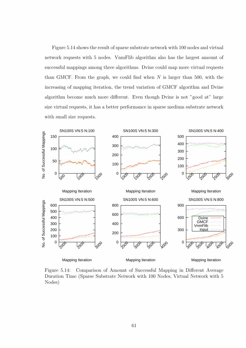
Figure 5.14 shows the result of sparse substrate network with 100 nodes and virtual

network requests with 5 nodes. VnmFlib algorithm also has the largest amount of

successful mappings among three algorithms. Dvine could map more virtual requests

than GMCF. From the graph, we could find when N is larger than 500, with the

increasing of mapping iteration, the trend variation of GMCF algorithm and Dvine

algorithm become much more different. Even though Dvine is not ”good at” large

size virtual requests, it has a better performance in sparse medium substrate network

with small size requests.

0

50

100

150

500

100

0 1

500

No.

of S

ucce

ssfu

l Map

ping

s

Mapping Iteration

SN100S VN:5 N:100

0

100

200

300

400

100

0 1

500

200

0 2

500

Mapping Iteration

SN100S VN:5 N:300

0

100

200

300

400

500

150

0 2

000

250

0 3

000

Mapping Iteration

SN100S VN:5 N:400

0

100

200

300

400

500

600

200

0 2

500

300

0

No.

of S

ucce

ssfu

l Map

ping

s

Mapping Iteration

SN100S VN:5 N:500

0

200

400

600

800

250

0 3

000

350

0 4

000

Mapping Iteration

SN100S VN:5 N:600

0

300

600

900

300

0 3

500

400

0 4

500

500

0

Mapping Iteration

SN100S VN:5 N:800

DvineGMCF

VnmFlibInput

Figure 5.14: Comparison of Amount of Successful Mapping in Different AverageDuration Time (Sparse Substrate Network with 100 Nodes, Virtual Network with 5Nodes)

61

Figure 5.15 shows the result of sparse substrate network with 100 nodes and vir-

tual network requests with 10 nodes. We could find the successful mapping amount

of GMCF is larger than Dvine and VnmFlib algorithm also has the highest amoun-

t. Compared with the medium dense substrate network, the amount of successful

mappings in sparse substrate network are much smaller, especially when N equal

to 700. For details, the amount of successful mappings of VnmFlib is 675 (totally

4000), which is 3 times than GMCF and 3.85 times than Dvine in dense substrate

network; the amount of successful mappings of VnmaFlib is 504 (totally 4000), which

is 2.65 times than GMCF and 4 times than Dvine. The dense substrate has a higher

node degree than sparse substrate, which could offer more link resources for virtual

requests.

0

20

40

60

80

500

750

100

0

No.

of S

ucce

ssfu

l Map

ping

s

Mapping Iteration

SN100S VN:10 N:50

0

50

100

150

100

0 1

500

200

0

Mapping Iteration

SN100S VN:10 N:100

0

75

150

225

800

140

0 2

000

Mapping Iteration

SN100S VN:10 N:200

DvineGMCF

VnmFlibInput

0

90

180

270

360

450

200

0 2

500

300

0

No.

of S

ucce

ssfu

l Map

ping

s

Mapping Iteration

SN100S VN:10 N:400

0

200

400

600

300

0 3

500

400

0

Act

ive

Suc

cess

ful M

appi

ng R

eque

sts

Mapping Iteration

SN100S VN:10 N:500

0

200

400

600

800

300

0 3

500

400

0

Act

ive

Suc

cess

ful M

appi

ng R

eque

sts

Mapping Iteration

SN100S VN:10 N:700

Figure 5.15: Comparison of Amount of Successful Mapping in Different AverageDuration Time (Sparse Substrate Network with 100 Nodes, Virtual Network with 10Nodes)

62

Figure 5.16 shows the result of dense substrate network with 500 nodes and virtual

network requests with 5 nodes. We could find when N is smaller than 300, all of three

algorithms have a good performance, the amount of successful mappings are approach

to the input. VnmFlib could almost handle all requests successfully even though N is

increasing to 1000. When N is smaller than 300, GMCF and Dvine have the similar

variation tendency. When N is increasing to 400, the amount of successful mappings

of Dvine is 1.5 times than GMCF. Compare with the medium substrate network,

Dvine is more suitable to the large substrate network.

0

100

200

300

100

0 1

500

200

0

No.

of S

ucce

ssfu

l Map

ping

s

Mapping Iteration

SN500D VN:5 N:200

0

100

200

300

400

150

0 2

000

250

0 3

000

Mapping Iteration

SN500D VN:5 N:300

DvineGMCF

VnmFlibInput

0

100

200

300

400

500

200

0 2

500

300

0

Mapping Iteration

SN500D VN:5 N:400

0

200

400

600

150

0 2

000

250

0 3

000

No.

of S

ucce

ssfu

l Map

ping

s

Mapping Iteration

SN500D VN:5 N:600

0

200

400

600

800

1000

200

0 2

500

300

0 3

500

400

0

Mapping Iteration

SN500D VN:5 N:900

0

200

400

600

800

1000

300

0 3

500

400

0 4

500

500

0

Mapping Iteration

SN500D VN:5 N:1000

Figure 5.16: Comparison of Amount of Successful Mapping in Different AverageDuration Time (Dense Substrate Network with 500 Nodes, Virtual Network with 5Nodes)

63

Figure 5.17 shows the result of sparse substrate network with 500 nodes and

virtual network requests with 5 nodes. When N is smaller than 300, VnmFlib could

almost map all requests successfully and GMCF, Dvine could successful handle more

than half of input requests. When N is increasing to 500, the amount of successful

mapping of GMCF is 908 (total 4000) and Dvine is 1181 (total 4000), which is only

a quarter of input requests. In the sparse substrate network, the node degree is only

half of dense substrate network. There are less opportunity for mapping algorithms

to find the optimized mapping solutions. Dvine is also has a better performance than

GMCF and VnmFlib still has the highest amount of successful mappings.

0

100

200

300

100

0 1

500

200

0

No.

of S

ucce

ssfu

l Map

ping

s

Mapping Iteration

SN500S VN:5 N:200

0

100

200

300

400

200

0 2

500

300

0

Mapping Iteration

SN500S VN:5 N:300

0

100

200

300

400

500

600

200

0 2

500

300

0

Mapping Iteration

SN500S VN:5 N:500

0

200

400

600

800

150

0 2

000

250

0 3

000

No.

of S

ucce

ssfu

l Map

ping

s

Mapping Iteration

SN500S VN:5 N:700

0

200

400

600

800

1000

200

0 2

500

300

0 3

500

400

0

Mapping Iteration

SN500S VN:5 N:900

0

200

400

600

800

1000

300

0 3

500

400

0 4

500

500

0

Mapping Iteration

SN500S VN:5 N:1000

DvineGMCF

VnmFlibInput

Figure 5.17: Comparison of Amount of Successful Mapping in Different AverageDuration Time (Sparse Substrate Network with 500 Nodes, Virtual Network with 5Nodes)

64

5.3.2 Comparison of Different Average Amount of Active Requests

Figure 5.18 to Figure 5.22 show the average successful mapping amount respect

to average amount of active requests in the substrate network. The x-axis is the av-

erage amount of active requests ”stay” in the substrate network, the y-axis is average

successful mapping amount of each algorithms. We also draw the ”input” line, which

is the ”perfect” result, all of the requests have mapped successfully. We will discuss

the every graph in the following:

Figure 5.18 shows the comparison of average successful mappings in dense sub-

strate network with 100 nodes and virtual network with 5 nodes. We could find

VnmFlib algorithm mostly approach the input line, which has the largest amount of

successful mappings. Dvine and GMCF algorithm almost has the same variant trend

when N is smaller than 800, with the increasing of N , the difference between them

become obvious.

0

200

400

600

800

1000

0 200 400 600 800 1000

Ave

rage

Suc

cess

ful M

appi

ng A

mou

nt

Average Amount of Active Requests

SN100D Link255; VN:Node5

DvineGMCF

VnmFlibInput

Figure 5.18: Comparison of Different Average Amount of Active Requests (DenseSubstrate Network with 100 Nodes, Virtual Network with 5 Nodes)

65

Figure 5.19 shows the comparison of average successful mappings in the same

substrate network like above with 10-node requests. VnmFlib algorithm could han-

dle almost all the requests until N larger than 500. GMCF algorithm has a higher

successful mapping amount than Dvine algorithm. We could find the difference be-

tween GMCF algorithm and Dvine algorithm become obvious when N is equal to

500. Compared with the Figure 5.18, N is smaller when appears obvious difference,

because it it more difficult for algorithms to find the mapping solutions when the size

of requests become larger.

0

100

200

300

400

500

600

700

800

0 100 200 300 400 500 600 700 800

Ave

rage

Suc

cess

ful M

appi

ng A

mou

nt

Average Amount of Active Requests

SN100D Link255; VN:Node10

DvineGMCF

VnmFlibInput

Figure 5.19: Comparison of Different Average Amount of Active Requests (DenseSubstrate Network with 100 Nodes, Virtual Network with 10 Nodes)

66

Figure 5.20 shows the result of medium dense substrate network with 20-node re-

quests. From the graph, we could find the GMCF algorithm is much more approach

to the input line than the former situation (mapping 5-node requests and 10-node

requests). For the details, we could find all the failed mapping requests due to the

failed link mapping for GMCF. With the increasing of N , the amount of success-

ful mappings of VnmFlib rise faster than GMCF. When N is larger than 350, the

difference between GMCF and VnmFlib becomes larger.

0

50

100

150

200

250

300

350

400

450

0 50 100 150 200 250 300 350 400 450

Ave

rage

Suc

cess

ful M

appi

ng A

mou

nt

Average Amount of Active Requests

SN100D Link255; VN:Node20

GMCFVnmFlib

Input

Figure 5.20: Comparison of Different Average Amount of Active Requests (DenseSubstrate Network with 100 Nodes, Virtual Network with 20 Nodes)

67

Figure 5.21 shows the result of medium sparse substrate network with 5-node

requests. From the graph, we could find VnmFlib also has the best performance

among three algorithms. Dvine could map more virtual requests than GMCF, but

the slope of straight line of GMCF is increasing and the slope of straight line of Dvine

is decreasing and tends to steady. There is obvious difference between GMCF and

Dvine when N is equal to 350, however, in dense substrate network, the variation

trend of these two algorithms almost the same until N equal to 800. Because it is

easier for algorithms to find the optimal mapping resources in the higher node degree

network, most of algorithms could handle the requests when average amount of active

requests is small in the substrate network. When node degree is smaller, it is more

difficult to find the solution even though the value of N is small.

0

100

200

300

400

500

600

700

800

0 100 200 300 400 500 600 700 800

Ave

rage

Suc

cess

ful M

appi

ng A

mou

nt

Average Amount of Active Requests

SN100S Link129; VN:Node5

DvineGMCF

VnmFlibInput

Figure 5.21: Comparison of Different Average Amount of Active Requests (SparseSubstrate Network with 100 Nodes, Virtual Network with 5 Nodes)

68

Figure 5.22 shows the result of medium sparse substrate network with 10-node

requests. Even though the VnmFlib algorithm most approach to the input line, the

slope of straight line is decreasing when N is bigger than 500, which is different from

the Figure 5.21. Dvine and GMCF algorithm tend to steady state when the average

amount of active requests is higher than 500 and GMCF also could successful map

more requests than Dvine.

0

100

200

300

400

500

600

700

0 100 200 300 400 500 600 700

Ave

rage

Suc

cess

ful M

appi

ng A

mou

nt

Average Amount of Active Requests

SN100S Link129; VN:Node10

DvineGMCF

VnmFlibInput

Figure 5.22: Comparison of Different Average Amount of Active Requests (SparseSubstrate Network with 100 Nodes, Virtual Network with 10 Nodes)

69

5.3.3 Conclusion of Experiment Results

Overall, in the dynamic VNMBench model, VnmFlib algorithm has the highest

successful mapping amount in the situation of different average amount of active

requests. It also has the shortest running time among the three algorithms when node

of requests is 5. With the increasing of average amount of active requests, VnmFlib

still could handle most of the requests and its line approach to the input line. So

VnmFlib algorithm is the best choice to resolve the virtual network mapping problem

in dynamic VNMBench model with both medium and large substrate network.

For GMCF algorithm and Dvine algorithm, they have the similar successful map-

ping amount and variant tendency in dynamic model when amount of success mapping

requests is small. With the increasing of value of N , the difference between them be-

comes obvious. Dvine is more suitable for the small size virtual requests and GMCF

has better performance in the large size virtual requests. For the large size substrate

network, Dvine could map more requests than GMCF when virtual requests in small

size. In additional, Dvine takes the longest running time among the three algorithm-

s. For example, its running time is almost 5 times than VnmFlib and 3 times than

GMCF in dense medium substrate network with 5-node requests. GMCF has the

shortest running time when requests node is 10, so for the medium size requests,

if we emphasis the running time, GMCF is a better choice. There is more obvious

difference among three algorithms using sparse medium substrate network than using

dense medium substrate network in the dynamic VNMBench model.

70

CHAPTER 6

CONCLUSION

Network virtualization is a way of sharing a physical network among virtual net-

works that can differ in functionality. The mapping of virtual network requests to

physical resources is an important aspect of operation of a virtual network system.

Various mapping algorithms have been developed in literature, but a detailed quan-

titative understanding of their performance has been difficult due to differences in

their performance evaluation.

In our work, we introduce VNMBench, a benchmark for evaluation virtual net-

work mapping algorithms that allows thorough evaluation and comparison of these

algorithms. We discuss the design of the benchmark, its inputs, and its performance

metrics. In order to better evaluate the mapping algorithms, we separate our model

into static and dynamic. For static VNMBench model, all requests are mapped suc-

cessively onto a substrate without ever removing (or changing) a mapping that has

been completed. It could test the performance of algorithms when there are limit-

ed resources in the substrate network. Similar to the situation that most customers

occupy the network resources for a long time to do the experiments, the mapping

algorithm need to find the optimized solution for the next request in the limited re-

sources. For dynamic VNMBench model, each request has a lifetime, they will be

moved from the substrate network and release their resources when they expire. Sim-

ilar to the situation that a service provider may deploy a new service at any time, and

continue supporting the service indefinitely, possibly discontinuing the service when

it is no longer profitable. We evaluate three different algorithms using VNMBench

71

and show that detailed performance results and comparisons between algorithms can

be achieved. We also show that the results obtained when using VNMBench are

comparable to those from real Emulab requests.

From the experiment results, we could find mapping algorithms have different

performance in the static model and dynamic model in different metrics. Such as

even though VnmFlib has the highest amount of successful mappings in both model,

it takes much higher running time in the static VNMBench model than in the dynamic

VNMBench model. GMCF could successful handle more requests than Dvine in

static VNMBench model in medium size, but Dvine has a better performance than

GMCF in dynamic VNMBench model in large size. We provide a detailed model

to compare different mapping algorithms and user could choose the most suitable

mapping algorithm based on the different evaluation results. For the new mapping

algorithms, in the static model, we think they need to consider how to improve

the running time when they maintain a highest successful mapping amount. In the

dynamic model, the new mapping algorithm need to consider how to improve the

amount of successful mappings when the size of virtual network requests is large.

We believe that our work provides an important foundation to quantitatively eval-

uating the performance of a critical component in the operation of virtual networks,

and presents an important step toward finding faster and more effective virtual net-

work mapping algorithms in the future.

72

BIBLIOGRAPHY

[1] Andersen, David G. Theoretical approaches to node assignment. Tech. Rep.

Paper 86, Department of Computer Science, Carnegie Mellon University, Pitts-

burgh, PA, Dec. 2002.

[2] Anderson, Thomas, Peterson, Larry, Shenker, Scott, and Turner, Jonathan.

Overcoming the Internet impasse through virtualization. Computer 38, 4 (Apr.

2005), 34–41.

[3] Carapinha, J., and Jimenez, J. Network virtualization: a view from the bottom.

ACM SIGCOMM Workshop on Virtualized Infastructure Systems and Architec-

tures (VISA) (Aug 2009), 73–80.

[4] Chen, Qian, Hyunseok, Qian Chen, Govindan, Ramesh, Jamin, Sugih, Shenker,

Scott J., and Willinger, Walter. The origin of power laws in internet topologies

revisited. In In IEEE INFOCOM 2002 (2002), pp. 608–617.

[5] Chen, Qian, Hyunseok, Qian Chen, Govindan, Ramesh, Jamin, Sugih, Shenker,

Scott J., and Willinger, Walter. The origin of power laws in internet topologies

revisited. In In IEEE INFOCOM 2002 (2002), pp. 608–617.

[6] Chowdhury, N. M. Mosharaf Kabir, and Boutaba, Raouf. A survey of network

virtualization. Computer Networks 54, 5 (Apr. 2010), 862–876.

[7] Chowdhury, N. M. Mosharaf Kabir, Rahman, Muntasir Raihan, and Boutaba,

Raouf. Virtual network embedding with coordinated node and link mapping. In

INFOCOM’09 (2009), pp. 783–791.

73

[8] Chowdhury, N.M.M.K., Rahman, M.R., and Boutaba, R. Virtual network em-

bedding with coordinated node and link mapping. In IEEE INFOCOM (2009),

pp. 5634–5640.

[9] Clark, D. Policy routing in internet protocols. Tech. Rep. RFC1102, M.I.T.

Laboratory for Computer Science, 1989.

[10] Clark, David D. The design philosophy of the DARPA Internet protocols. In

Proc. of ACM SIGCOMM 88 (Stanford, CA, Aug. 1988), pp. 106–114.

[11] Cordella, L. P., Foggia, P., Sansone, C., and Vento, M. An improved algorith-

m for matching large graphs. In 3rd IAPR-TC15 Workshop on Graph-based

Representations in Pattern Recognition, Cuen (2001), pp. 149–159.

[12] Doar, Matthew, and Leslie, Ian M. How bad is naıve multicast routing? In

INFOCOM (1993), pp. 82–89.

[13] Egevang, Kjeld Borch, and Francis, Paul. The IP network address translator

(NAT). RFC 1631, Network Working Group, May 1994.

[14] Fan, Jinliang, and Ammar, Mostafa H. Dynamic topology configuration in ser-

vice overlay networks: A study of reconfiguration policies. In In Proc. IEEE

INFOCOM (2006).

[15] Feldmann, Anja, Kind, Mario, Maennel, Olaf, Schaffrath, Gregor, and Wer-

le, Christoph. Network virtualization - an enabler for overcoming ossification.

ERCIM News 2009, 77 (2009).

[16] Guha, Saikat, and Francis, Paul. An end-middle-end approach to connection

establishment. In SIGCOMM ’07: Proceedings of the 2007 conference on Appli-

cations, technologies, architectures, and protocols for computer communications

(Kyoto, Japan, Aug. 2007), pp. 193–204.

74

[17] Jacobson, Van, Smetters, Diana K., Thornton, James D., Plass, Michael F.,

Briggs, Nicholas H., and Braynard, Rebecca L. Networking named content. In

Proceedings of the 5th international conference on Emerging networking experi-

ments and technologies (CoNEXT) (Rome, Italy, Dec. 2009), pp. 1–12.

[18] J.lu, and J.Turner. Efficient mapping of virtual networks onto a shared substrate.

[19] John D.C. Little, Stephen C. Graves. Little’s law. pp. 81–100.

[20] Lischka, J., and Karl, H. A virtual network mapping algorithm based on sub-

graph isomorphism detection. In Proceedings of the 1st ACM workshop on Vir-

tualized infrastructure systems and architectures (Aug 2009), ACM New York,

NY, USA, pp. 81–88.

[21] Matthew Doar, Ian Leslie. How bad is naive multicast routing? In Twelfth

Annual Joint Conference of the IEEE Computer and Communications Societies.

Networking: Foundation for the Future. (San Francisco, CA, August 1993), p-

p. 82–89.

[22] Mogul, Jeffrey C. Simple and flexible datagram access controls for UNIX-based

gateways. In USENIX Conference Proceedings (Baltimore, MD, June 1989),

pp. 203–221.

[23] Ratnasamy, Sylvia, Francis, Paul, Handley, Mark, Karp, Richard, and Schenker,

Scott. A scalable content-addressable network. In SIGCOMM ’01: Proceedings

of the 2001 conference on Applications, technologies, architectures, and protocols

for computer communications (New York, NY, USA, 2001), ACM, pp. 161–172.

[24] Schrijver, Alexander. Theory of linear and integer programming. John Wiley &

Sons, Inc., New York, NY, USA, 1986.

75

[25] Szeto, W., Iraqi, Y., and Boutaba, R. A multi-commodity flow based approach to

virtual network resource allocation. In Global Telecommunications Conference,

2003. GLOBECOM ’03. IEEE (2003), vol. 6, pp. 3004 – 3008 vol.6.

[26] Tangmunarunkit, Hongsuda, Govindan, Ramesh, Jamin, Sugih, Shenker, Scott,

and Willinger, Walter. Network topology generators: Degree-based vs. struc-

tural. In In Proceedings of ACM SIGCOMM (2002), pp. 147–159.

[27] Turner, Jonathan S., and Taylor, David E. Diversifying the Internet. In Proc.

of IEEE Global Communications Conference (GLOBECOM) (Saint Louis, MO,

Nov. 2005), vol. 2.

[28] Waxman, Bernard M. Broadband switching: architectures, protocols, design,

and analysis. IEEE Computer Society Press, 1991, ch. Routing of multipoint

connections, pp. 347–352.

[29] Waxman, Bernard M. Routing of multipoint connections. IEEE Computer Soci-

ety Press, Los Alamitos, CA, USA, 1991, pp. 347–352.

[30] Wei, L., and Estrin, D. The trade-offs of multicast trees and algorithms, 1994.

[31] Wei, Liming, and Estrin, Deborah. The trade-offs of multicast trees and algo-

rithms.

[32] White, Brian, Lepreau, Jay, Stoller, Leigh, Ricci, Robert, Guruprasad, Shashi,

Newbold, Mac, Hibler, Mike, Barb, Chad, and Joglekar, Abhijeet. An integrated

experimental environment for distributed systems and networks. In Proc. of the

Fifth Symposium on Operating Systems Design and Implementation (Boston,

MA, Dec. 2002), USENIX Association, pp. 255–270.

[33] Willinger, W, Govindan, R, Jamin, S, Paxson, V, and Shenker, S. Scaling phe-

nomena in the Internet: Critically examining criticality. vol. 99, pp. 2573–2580.

76

[34] Yu, M., Yi, Y., Rexford, J., and Chiang, M. Rethinking virtual network em-

bedding: substrate support for path splitting and migration. ACM SIGCOMM

CCR 38, 2 (April 2008), 17–29.

[35] Yu, Minlan, Yi, Yung, Rexford, Jennifer, and Chiang, Mung. Rethinking vir-

tual network embedding: substrate support for path splitting and migration.

SIGCOMM Comput. Commun. Rev. 38 (March 2008), 17–29.

[36] Zegura, E., Calvert, K., and Bhattacharjee, S. How to model an internetwork.

In Proceedings of IEEE INFOCOM (1996), pp. 594–602.

[37] Zegura, Ellen, Calvert, Kenneth, and Bhattacharjee, Samrat. How to model an

internetwork. In Proc. of the Fifteenth IEEE Conference on Computer Commu-

nications (INFOCOM) (San Francisco, CA, Mar. 1996), pp. 594–602.

[38] Zegura, Ellen W., Calvert, Kenneth L., and Bhattacharjee, Samrat. How to

model an internetwork. In Proceedings of the Fifteenth annual joint conference

of the IEEE computer and communications societies conference on The confer-

ence on computer communications - Volume 2 (Washington, DC, USA, 1996),

INFOCOM’96, IEEE Computer Society, pp. 594–602.

[39] Zegura, Ellen W., Calvert, Kenneth L., and Donahoo, Michael J. A quantitative

comparison of graph-based models for internet topology. IEEE/ACM Trans.

Netw. 5 (December 1997), 770–783.

[40] Zhu, Y., and Ammar, M. Algorithms for assigning substrate network resources

to virtual network components. In IEEE INFOCOMM (April 2006), pp. 1–12.

77