benchmarking in a rotating annulus: a comparative

BMeteorologische Zeitschrift, Vol. 23, No. 6, 611–635 (published online January 13, 2015) Open Access Article© 2014 The authors

Benchmarking in a rotating annulus: a comparativeexperimental and numerical study of baroclinic wavedynamics

Miklos Vincze1, Sebastian Borchert2, Ulrich Achatz2, Thomas von Larcher3, MartinBaumann4, Claudia Liersch5, Sebastian Remmler6, Teresa Beck4, Kiril D. Alexandrov1,Christoph Egbers1, Jochen Fröhlich5, Vincent Heuveline4, Stefan Hickel6 and UweHarlander1∗

1Lehrstuhl für Aerodynamik und Strömungslehre, Brandenburgische Technische Universität Cottbus-Senftenberg,Cottbus, Germany2Institut für Atmosphäre und Umwelt, Goethe-Universität at Frankfurt am Main, Frankfurt am Main, Germany3Institut für Mathematik, Freie Universität Berlin, Berlin, Germany4Engineering Mathematics and Computing Lab (EMCL), Interdisziplinäres Zentrum für WissentschaftlichesRechnen, Universität Heidelberg, Heidelberg, Germany5Institut für Strömungsmechanik, Technische Universität Dresden, Dresden, Germany6Lehrstuhl für Aerodynamik und Strömungsmechanik, Technische Universität München, München, Germany

(Manuscript received March 7, 2014; in revised form August 11, 2014; accepted October 1, 2014)

AbstractThe differentially heated rotating annulus is a widely studied tabletop-size laboratory model of the generalmid-latitude atmospheric circulation. The two most relevant factors of cyclogenesis, namely rotation andmeridional temperature gradient are quite well captured in this simple arrangement. The radial temperaturedifference in the cylindrical tank and its rotation rate can be set so that the isothermal surfaces in the bulk tilt,leading to the formation of baroclinic waves. The signatures of these waves at the free water surface have beenanalyzed via infrared thermography in a wide range of rotation rates (keeping the radial temperature differenceconstant) and under different initial conditions. In parallel to the laboratory experiments, five groups of theMetStröm collaboration have conducted numerical simulations in the same parameter regime using differentapproaches and solvers, and applying different initial conditions and perturbations. The experimentally andnumerically obtained baroclinic wave patterns have been evaluated and compared in terms of their dominantwave modes, spatio-temporal variance properties and drift rates. Thus certain “benchmarks” have been createdthat can later be used as test cases for atmospheric numerical model validation.

Keywords: benchmark, baroclinic instability, rotating annulus

1 Introduction

In the endeavor to improve weather forecasting andclimate prediction techniques, the validation and fine-tuning of numerical models of large-scale atmosphericprocesses play clearly crucial roles. However, in such acomplex system as the real atmosphere, validation testsare especially difficult to perform. Besides the issuesthat arise due to coarse-graining – a central problem ofthe numerical modeling of any hydrodynamic problem –in the case of atmospheric processes the unavoidable im-perfection of the governing equations themselves is alsoa considerable source of inaccuracies. In the commonlyapplied hydro-thermodynamic equations the unresolved(or even physically not properly understood) processes

∗Corresponding author: Uwe Harlander, Lehrstuhl für Aerodynamik undStrömungslehre, Brandenburgische Technische Universität Cottbus – Senf-tenberg Lehrgebäude 3A, Siemens-Halske-Ring 14, 03046 Cottbus, Ger-many, e-mail: [email protected]

are either neglected or taken into account via empiri-cal parametrization. Thus, the separation of discretiza-tion errors from the ones originating from the theoreticalformulation of a given model poses a real challenge toresearchers.

Yet, there is a way to carry out systematic and re-producible tests under controlled circumstances, and tocapture a large segment of the complexity of these large-scale flows through relatively simple, tabletop-size ex-periments, based on the principle of hydrodynamic simi-larity. Under laboratory conditions it is possible to ad-just the governing physical parameters and thus to sep-arate different processes that cannot be studied inde-pendently in the real atmosphere. Therefore, labora-tory experiments provide a remarkable test bed to vali-date numerical techniques and models aiming to inves-tigate geophysical flows. This was one of the primarygoals of the German Science Foundation’s (DFG) prior-ity program MetStröm. Research focuses on the theoryand methodology of multiscale meteorological fluid me-

© 2014 The authorsDOI 10.1127/metz/2014/0600 Gebrüder Borntraeger Science Publishers, Stuttgart, www.borntraeger-cramer.com

http://www.borntraeger-cramer.de/journals/metz

http://www.borntraeger-cramer.de/journals/metz

http://www.borntraeger-cramer.com

612 M. Vincze et al.: Benchmarking in a rotating annulus Meteorol. Z., 23, 2015

chanics modelling and accompanying reference experi-ments supported model validation.

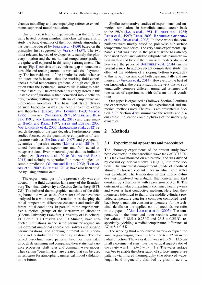
One of these reference experiments was the differen-tially heated rotating annulus. This classical apparatus tostudy the basic dynamics of the mid-latitude atmospherehas been introduced by Fultz et al. (1959) based on theprinciples first suggested by Vettin (1857). The twomost relevant factors of cyclogenesis, namely the plan-etary rotation and the meridional temperature gradientare quite well captured in this simple arrangement. Theset-up (Fig. 1) consists of a cylindrical gap mounted on aturntable and rotating around its vertical axis of symme-try. The inner side wall of the annulus is cooled whereasthe outer one is heated, thus the working fluid experi-ences a radial temperature gradient. At high enough ro-tation rates the isothermal surfaces tilt, leading to baro-clinic instability. The extra potential energy stored in thisunstable configuration is then converted into kinetic en-ergy, exciting drifting wave patterns of temperature andmomentum anomalies. The basic underlying physicsof such baroclinic waves has been subject of exten-sive theoretical (Eady, 1949; Lorenz, 1963; Mason,1975), numerical (Williams, 1971; Miller and But-ler, 1991; von Larcher et al., 2013) and experimen-tal (Früh and Read, 1997; Sitte and Egbers, 2000;Von Larcher et al., 2005; Harlander et al., 2012) re-search throughout the past decades. Furthermore, somestudies focused on the quantitative comparison of tem-perature statistics (Gyüre et al., 2007) and propagationdynamics of passive tracers (Jánosi et al., 2010) ob-tained from annulus experiments and from actual at-mospheric data. Even meteorological data assimilationtechniques (Ravela et al., 2010; Young and Read,2013) and techniques operational in meteorological en-semble prediction (Young and Read, 2008; Harlan-der et al., 2009; Hoff et al., 2014) have also been stud-ied by using annulus data.

The experimental part of the present study was con-ducted in the fluid dynamics laboratory of the Branden-burg Technical University at Cottbus-Senftenberg (BTUCS). The infrared thermographic snapshots of the drift-ing baroclinic waves at the free water surface have beenanalyzed in a wide range of rotation rates (keeping theradial temperature difference constant) and under dif-ferent initial conditions. In parallel to the experiments,five numerical groups of the MetStröm collaboration(Goethe University Frankfurt, University of Heidelberg,FU Berlin, TU Dresden and TU Munich) have con-ducted simulations in the same parameter regime us-ing different numerical approaches, solvers and subgridparametrizations, and applying different initial condi-tions and perturbations for stability analysis. The ob-tained baroclinic wave patterns have been evaluatedthrough determining and comparing their statistical vari-ance properties, drift rates and dominant wave modes.Thus certain “benchmarks” are created that can be usedas test cases for atmospheric numerical model validationin the future.

Similar comparative studies of experiments and nu-merical simulations in baroclinic annuli stretch backto the 1980s (James et al., 1981; Hignett et al., 1985;Read et al., 1997; Read, 2003; Randriamampianinaet al., 2006; Read et al., 2008). In these works the com-parisons were mostly based on pointwise sub-surfacetemperature time series. The very same experimental ap-paratus that was used in the present work has alreadybeen used to test and validate subgrid-scale parametriza-tion methods of two of the numerical models also usedhere (see the paper of Borchert et al. (2014) in thepresent issue). In another recent comparative study, theeffect of the addition of a sloping bottom topographyto this set-up was analyzed both experimentally and nu-merically (Vincze et al., 2014). However, to the best ofour knowledge, the present study is the very first to sys-tematically compare different numerical schemes andtwo series of experiments with different initial condi-tions.

Our paper is organized as follows. Section 2 outlinesthe experimental set-up, and the experimental and nu-merical methods used. The results are presented in Sec-tion 3. In Section 4 we summarize the results and dis-cuss their implications on the physics of the underlyingdynamics.

2 Methods

2.1 Experimental apparatus and procedures

The laboratory experiments of the present study havebeen conducted in the baroclinic wave tank of BTU CS.This tank was mounted on a turntable, and was dividedby coaxial cylindrical sidewalls (Fig. 1) into three sec-tions. The innermost compartment (made of anodizedaluminum) housed coolant pipes in which cold waterwas circulated. The temperature in this middle cylin-der was monitored via a digital thermometer and keptconstant by a thermostat with a precision of 0.05 K. Theoutermost annular compartment contained heating wiresand water as heat conductive medium. Here four ther-mometers (identical to that of the middle cylinder) pro-vided temperature data for a computer-controlled feed-back loop to maintain constant temperature; for the tech-nical details on the applied control methods we referto the paper of Von Larcher et al. (2005). The tem-peratures in the inner and outer sections were set tothe values of 18.5 ± 0.25 °C and 26.5 ± 0.25 °C, re-spectively, yielding a radial temperature difference ofΔT = 8 ± 0.5 K.

The working fluid – de-ionized water – occupied theannular gap ranging from a = 4.5 cm to b = 12 cm in theradial direction. The water depth was set to D = 13.5 cmin all experimental runs, thus the vertical aspect ratio ofthe cavity was Γ = D/(b − a) = 1.8. The water surfacewas free to enable the observation of surface temperaturepatterns via infrared thermography (the observed wave-length band is generally absorbed by glass or acrylic,

Meteorol. Z., 23, 2015 M. Vincze et al.: Benchmarking in a rotating annulus 613

Figure 1: Schematic drawing of the laboratory set-up. For thevalues of the geometric parameters shown, see the text. The counter-clockwise direction of rotation is indicated.

thus covering the tank with a rigid lid was not possible).The physical properties of the fluid are characterized byits kinematic viscosity ν = 1.004 × 10−6 m2/s and itsthermal conductivity κ = 0.1434× 10−6 m2/s, yielding aPrandtl number of Pr ≡ ν/κ ≈ 7.0.

Since the temperature difference ΔT as well as theaforementioned geometric and material quantities werekept constant throughout the experiments, rotation rate(i.e. angular velocity) Ω was the single control parameterto be adjusted between the subsequent runs. The mini-mum rotation rate investigated was Ωmin = 2.26 rpm(revolutions per minute), where the flow was found tobe axially symmetric, i.e. its radial and vertical struc-ture was independent from azimuthal angle θ, indicatingthe absence of baroclinic instability. The highest inves-tigated rotation rate was Ωmax = 20.91 rpm. Here, four-fold symmetric baroclinic wave patterns were observed(see the exemplary thermographic snapshots of Fig. 2).Within the interval ranging from Ωmin to Ωmax, our mea-surements were taken at 17 different rotation rates. Foreach of these cases, two types of initial conditions wereapplied: the so-called “spin-up” and “spin-down” se-quences. In the former (latter) initialization procedurethe target rotation rate Ω was approached starting fromthe previously studied smaller (higher) rotation rate Ωi,with |Ω − Ωi| ≈ 1 rpm. The rotation rate was then grad-ually increased (decreased) by δΩ ≈ 0.1 rpm in every2 minutes; thus, it took approximately 20 minutes toreach the required Ω from Ωi. 10 minutes after arriv-ing at Ω the data acquisition started and lasted for 40to 80 minutes in each case. Afterwards this gradual in-creasing (decreasing) procedure of the rotation rate con-tinued in order to reach the next Ω, with the previous pa-rameter point as Ωi, providing a long “spin-up” (“spin-down”) experiment series. Thus, in total 17×2 measure-ments were performed and evaluated. Note, that in or-der to enable the standard initialization procedures at the

Figure 2: Four typical thermographic snapshots of surface tempera-ture patterns in the rotating annulus. a) An axially symmetric (m = 0)pattern at Ω = 2.28 rpm; b) A two-fold symmetric (m = 2) baro-clinic wave at Ω = 3.23 rpm; c) m = 3 at Ω = 4.20 rpm; d) m = 4 atΩ = 6.16 rpm (ΔT = 8 K).

end parameter points Ωmin and Ωmax, the initial value Ωiwas set smaller than Ωmin or larger than Ωmax, when re-quired. However, no data acquisition took place at these“out-of-range” parameter points.

The infrared camera was mounted above the middleof the tank and was fixed in the laboratory frame (notco-rotating). In every Δt = 2 s, 640 × 480-pixel thermo-graphic snapshots were taken, providing a precision ofaround 0.03 K for temperature differences. The obtainedtemperature fields can be considered surface tempera-ture patterns, since the penetration depth of the appliedwavelength into water is measured in millimeters. Thecaptured snapshots were acquired and stored by a com-puter, where they were converted to ASCII arrays (byorganizing the temperature values from all pixels intomatrix format) for further evaluation.

The most important classic non-dimensional pa-rameters widely used to compare the results obtainedfrom different baroclinic annulus set-ups are the Taylornumber Ta and thermal Rossby number RoT (alsoknown as Hide number). The former is basically a non-dimensional measure of rotation rate Ω and reads as

Ta =4Ω2(b − a)5

ν2D, (2.1)

whereas RoT expresses the ratio of the characteristicvelocity of the thermally driven flow to the rotation ratein the form of

RoT =DgαΔT

Ω2(b − a)2, (2.2)


Figure 3: The neutral stability curve (thick blue line) in the pa-rameter plane of T a and RoT , as obtained via linear stability analy-sis by von Larcher et al. (2013), using the geometrical and mate-rial parameters of the BTU C-S wave tank. The dotted line corre-sponding to the studied radial temperature difference ΔT = 8 K isalso indicated, along with the experimental data points (squares) andthe benchmark parameter points (circles) of the present comparativestudy (see text).

where g is the acceleration due to gravity and α = 2.07×10−4 K−1 represents the volumetric thermal expansioncoefficient of the working fluid. Note, that when thehorizontal temperature difference ΔT is comparable tothe vertical one, i.e. ΔTz ≈ ΔT holds (a fairly goodassumption in the present study), (2.2) corresponds tothe Burger number B, defined as the squared ratio ofthe Rossby deformation radius Rd =

√gdαΔTz/Ω to the

gap width b − a, B = gdαΔTz/(Ω2(b − a)2).In the case of the present study where the experi-

ments were conducted at a practically constant value ofΔT , an inverse proportionality Ro ∝ Ta−1 holds; thus ei-ther one of these parameters per se sufficiently describesthe applied conditions. Nevertheless, to demonstrate thebroader context of the studied domain, we present a con-ceptual Ta − RoT regime diagram in Fig. 3. The anvil-shaped thick (blue) curve represents the layout of the so-called neutral stability curve (as obtained numerically byvon Larcher et al. (2013), to the left of which the flowis axially symmetric (radial “sideways convection”). Tothe right of the curve, the emergence of steady baro-clinic wave patterns (as the ones in Fig. 2b, c and d)characterizes the flow, which – for even higher valuesof Ta – become irregular in shape as the system ap-proaches geostrophic turbulence (a state not studied inthe present paper). The curve corresponding to the con-stant radial temperature difference ΔT = 8 K that laywithin the focus of the present work is also indicated (by

a dotted curve), along with the experimental parameterpoints and the four benchmark points (to be addressedlater).

2.2 Numerical methods

In this subsection we briefly describe the different nu-merical models and methods used for the numericalsimulations.

2.2.1 Governing equations and general numericalproperties

The applied numerical models computed approximatesolutions of the hydrodynamic equations of motionin the Boussinesq approximation (Vallis, 2006), us-ing different initialization procedures, grids, time steps,boundary conditions and sub-grid–scale parametrizationschemes. The overall geometric parameters of the simu-lation domain corresponded to the aforementioned di-mensions of the annular cavity of the laboratory set-up.The governing equations themselves read as:

∂�u∂t

+ (�u · ∇)�u = −2Ω�ez × �u +δρ

ρ0Ω2r�er

− 1ρ0∇p +

δρ

ρ0g�ez + ν∇2�u, (2.3)

∇ · �u = 0, (2.4)∂T∂t

+ (�u · ∇)T = κ∇2T, (2.5)

where �er and �ez denote the unit vectors in the radialand vertical directions (pointing upwards), respectively,�u represents the velocity field, p is the pressure and δρdenotes the difference between the density of the givenfluid parcel and the reference density ρ0 (in the Boussi-nesq approximation |δρ| � ρ0 holds). The first and sec-ond terms on the right hand side of (2.3) account for theCoriolis and centrifugal forces, respectively, which – be-ing inertial forces – appear in the co-rotating referenceframe. This form of the equation was used in the im-plementations of the cylFloit, EULAG, and LESOCC2models. In INCA the centrifugal term was omitted, sinceit is generally negligible in the investigated parameterrange. For HiFlow3 the governing equations were solvedin the non-rotating “laboratory frame”, hence there bothinertial force terms were absent and the rotation of thetank entered the dynamics through the boundary condi-tions.

In all codes, the boundary conditions for the temper-ature were isothermal at the inner and outer sidewallsof the cavity (i.e. at radii r = a and r = b). The corre-sponding temperatures are denoted with T |r=a ≡ Ta andT |r=b ≡ Tb, respectively, yielding ΔT ≡ Tb−Ta = 8.0 K,in agreement with the laboratory set-up. On the top (z =D) and bottom (z = 0) boundaries no-flux conditionswere applied for the temperature (i.e. ∇T · �ez|z=0,D ≡ 0).For the velocities at the bottom and lateral sidewalls,the working fluid was assumed to co-rotate with the


Table 1: Summary of the basic properties of the applied numerical models.

cylFloit EULAG HiFlow3 INCA LESOCC2

reference frame co-rotating co-rotating non-rotating co-rotating co-rotating

centrifugal term? yes yes no no yes

Euler acceleration? yes no no no no

Initializationprocedure

spin-up/spin-down,with dynamic Ω(t)from the end stateof the previous run(at different Ω), orfrom non-rotatingaxisymmetric basicstate

rotation turned oninstantly

firstly, stationaryeqs. solved withincreased ν and κ,which then are setinstantly tophysically correctvalues

rotation turned oninstantly

rotation turned oninstantly, withinitial state“inherited” fromthe final state of theprevious run(different Ω)

temperatureboundaryconditions

Ta = 24 °CTb = 32 °C

Ta = 16 °CTb = 24 °C

Ta = 20 °CTb = 28 °C

Ta = 16 °CTb = 24 °C

Ta = 23.5 °CTb = 31.5 °C

isothermal at the sidewalls (Ta: inner, Tb: outer), no-flux at the top and bottom boundaries (∇T �ez|z=0,D ≡ 0)

velocity boundaryconditions

no-slip (�u ≡ 0) atthe bottom andsidewalls, free slip(�u · �ez = 0)at the top


rigid body rotationat all boundaries(�u = rΩ�eθ)



grid type regular cylindrical equidistantCartesian

cylindrical mesh Cartesian meshblocks

curvilinearCartesian mesh

number of gridpoints

40 × 60 × 50(r − θ − z)

192 × 192 × 67(x − y − z)

21 × 76 × 41(r − θ − z)

160 × 160 × 90(x − y − z)

1: 76 × 213 × 1372: 86 × 241 × 153(r − θ − z)

grid points total 120 000 2 469 888 65 436 2 304 000 1: 2 217 7562: 3 171 078

subgrid-scaleparametrization

ALDM n.a. n.a. ALDM n.a.

grid spacing(min./max.)

Δr : 1.88 mm rΔθ :4.71/12.57 mmΔz : 2.7 mm

Δx; Δy : 1.35 mmΔz : 2.04 mm

Δr :2.785/5.250 mmrΔθ :3.720/9.921 mmΔz :1.700/5.625 mm

Δx; Δy : 1.55 mmΔz : 0.4/1.8 mm

1: Δr : 0.6/1.4 mmrΔθ : 1.3/3.5 mmΔz : 0.6/1.1 mm2: Δr : 0.4/1.6 mmrΔθ : 1.2/3.1 mmΔz : 0.3/1.0 mm

integration timestep δt

〈δt〉 ≈ 0.1 s(adaptive)

0.0025 s 0.25 s 〈δt〉 ≈ 0.05 sadaptive in theinitial phase;afterwards:δt = 0.0375 s

1: 〈δt〉 ≈ 0.033 s2: 〈δt〉 ≈ 0.018 s(adaptive)

sample rate Δt 3 s; 5 s 5 s 0.25 s 5.625 s 1 s

tank (rigid body rotation). For the codes implementedin the co-rotating frame this yields no-slip conditions(�u|z=0 = �u|r=a = �u|r=b ≡ 0), whereas for HiFlow3 (non-rotating frame) this condition translates to �u|r = rΩ�eθfor r = a and r = b at all depths, and for all values of rat the bottom (z = 0). In all codes at the “free” water sur-face the slip conditions (∇u · �ez|z=D = ∇v · �ez|z=D ≡ 0) andw|z=D ≡ 0 were applied (u and v being the two horizontaland w the vertical velocity components).

The boundary conditions, reference frames, gridtypes and sizes and other general properties of the ap-

plied numerical codes are summarized in Table 1. In thefollowing subsections we briefly introduce these modelsand discuss their most important features.

2.2.2 cylFloit

The implementation of the cylindrical flow solver withimplicit turbulence model (cylFloit) is described inBorchert et al. (2014). The numerical model is basedon a finite-volume discretization of the governing equa-tions on a regular cylindrical grid. The subgrid-scale


turbulence is implicitly parameterized by the Adap-tive Local Deconvolution Method (ALDM), see Hickelet al. (2006). Time integration is done using the ex-plicit low-storage third-order Runge-Kutta method ofWilliamson (1980).

The temperature dependence of the density deviationδρ(T ), kinematic viscosity ν(T ) and thermal diffusiv-ity κ(T ) was approximated in the form of second-orderpolynomial fits to empirical reference data for the stud-ied temperature range. Because of this temperature de-pendence, ν and κ depend implicitly on space and time,which is the reason why the viscous stress and the heatconduction have slightly different forms than the right-most terms in (2.3) and (2.5). In order to simulate thespin-up and spin-down of the annulus, the Euler accel-eration −(dΩ/dt)r is added to the right-hand side of theazimuthal component of (2.3).

Three series of numerical simulations have been per-formed by cylFloit: the “from scratch” series (i), wherethe studied state at a target rotation rate Ω was reachedafter initializing the system from a non-rotating axiallysymmetric initial state; and the “spin-up” (ii) and “spin-down” (iii) series, where a rotation rate evolution Ω(t)similar to the aforementioned laboratory sequences wasimitated. The numerical parameters of these simulationsare listed in the second column of Table 1.

(i) The “from scratch” simulations: In this ini-tialization procedure, firstly an axially symmetric (thus,two dimensional; 2d) stationary solution was computedwithin a physical time of t2d = 10800 s (3 hrs), withΩ = 0, but with the aforementioned boundary condi-tions. To obtain an axially symmetric solution, the num-ber of azimuthal grid cells was set to Nθ = 1, thus re-ducing the problem to 2d. Then, starting from this statethe full 3d simulation was initialized with a spin-up fromzero angular velocity to its final value Ω f as:

Ω (t) =

⎧⎪⎪⎪⎪⎨⎪⎪⎪⎪⎩

0, 0 ≤ t ≤ t2dΩ f

2

{1 − cos

[πτ (t − t2d)

]}, t2d < t ≤ t2d + τ

Ω f , t > t2d + τ

.

(2.6)Here Ω f is the final constant angular velocity used inthe experiment and τ denotes the spin-up period of therotating annulus ranging from 20 s for Ωmin to 910 s forΩmax (Borchert et al., 2014). To trigger the formationof baroclinic waves, low amplitude random perturba-tions were added to the temperature field, with a max-imum amplitude of δTpert = 0.03|Tb −Ta|. This 3d simu-lation took another 10800 s, so that the waves could fullydevelop. A subsequent integration time of 7200 s (2 hrs)at maximum was used to record the data analysed in thepresent work. For further information on this initializa-tion method, we refer to Borchert et al. (2014).

(ii) Spin-up simulations: In these cases an initialangular velocity Ωi and a final angular velocity Ω f > Ωi

were chosen. The time evolution of the angular velocityΩ(t) was then computed according to the formula:

Ω (t) =

⎧⎪⎪⎨⎪⎪⎩Ωi +

Ω f −Ωi

2

{1 − cos

(π tτ′

)}, t ≤ τ′

Ω f , t > τ′, (2.7)

where τ′ means the spin-up or spin-down period. Thefirst simulation started with Ωi = 0 rpm and Ω f = 2 rpm,the second simulation used Ωi = 2 rpm and Ω f = 3 rpm,the third Ωi = 3 rpm and Ω f = 4 rpm and so forthup to the last spin-up simulation with Ωi = 19 rpmand Ω f = 20 rpm. The spin-up period was set to τ′ =1200 s (20 min) in order to imitate the typical spin-up time scale of the laboratory runs. After the spin-upperiod the simulation took another 1800 s (30 min). Eachsimulation was initialized with fields from the previoussimulation.

(iii) Spin-down simulations: The parameters andthe procedures of the spin-down series were the sameas for the spin-up runs, the only difference being that inthis case Ωi > Ω f holds. The first spin-down simulationwas initialized with the results from the last spin-upsimulation. It therefore used Ωi = 20 rpm and Ω f =19 rpm, the next Ωi = 19 rpm and Ω f = 18 rpm, andso forth down to Ωi = 2 rpm and Ω f = 0 rpm. After thespin-down period of τ′ = 1200 s the simulations heretook another 1200 s only, which was long enough forthe flow to equilibrate.

2.2.3 EULAG

The EULAG framework is a multipurpose multi scalesolver for geophysical flows, see Prusa et al. (2008)for a comprehensive review. The framework formu-lates the non-hydrostatic anelastic fluid equations of mo-tion, e.g., Grabowski and Smolarkiewicz (2002), thatcan be solved either in Eulerian flux form or in semi-Lagrangian advective form, and it allows for a number ofassumptions for particular flow characteristics, specif-ically the compressible/incompressible Boussinesq ap-proximation, incompressible Euler/Navier-Stokes equa-tions, and fully compressible Euler equations. The gov-erning partial differential equations are evaluated witha semi-implicit non-oscillatory forward-in-time (NFT)algorithm and a finite volume discretization (Smo-larkiewicz, 1991; Smolarkiewicz and Margolin,1997; Smolarkiewicz and Margolin, 1998). EULAGhas been successfully applied to a number of geophysi-cal problems, documented by the large number of pub-lications in the past years, see the list of publicationswith respect to applications on the EULAG model web-site at http://www.mmm.ucar.edu/eulag/pub_appl.html,ranging from cloud microscale to synoptic and globalscale in atmospheric flows, as well as it was used formodeling oceanic flows. It is worth mentioning that alsosolar convection (Elliott and Smolarkiewicz, 2002),and urban flows (Schröttle and Dörnbrack, 2013),were studied, moreover, EULAG has been also applied

http://www.mmm.ucar.edu/eulag/pub_appl.html


for simulating injuries of the human brain, treating it asa viscoelastic fluid (Cotter et al., 2002). Apart from thepossibility of considering particular flow characteristicsas mentioned above, EULAG also provides a frameworkfor Direct Numerical Simulation (DNS), Large EddySimulation (LES), and implicit LES (ILES). We here usethe DNS approach.

For the purposes of the present study the general EU-LAG framework has been adapted as follows. The side-walls and the end walls of the annulus were modeledwith the immersed boundary approach (cf. Goldsteinet al. (1993)), where fictitious body forces in the govern-ing equation of motion are incorporated to represent no-slip boundaries which leads to a damping of the solutionin an appropriate time interval. Smolarkiewicz et al.(2007) gives a detailed description of the implementa-tion of the immersed boundary approach in the EULAGflow solver. In our study, the damping parameters wereset so that the motion at the boundaries was damped tozero within a single time step. The properties of the grid,the time step and the boundary conditions are summa-rized in the third column of Table 1.

The governing equations (2.3) to (2.5) were solved inthe Boussinesq approximation on a Cartesian grid. Forthe ρ(T ) dependence a linear decrease of density withrespect to temperature was assumed with volumetricthermal expansion coefficient α = 2.07 × 10−4 K−1, asgiven at Tref = 20 °C. The Prandtl number was set toPr = 7, corresponding to the properties of de-ionizedwater.

2.2.4 HiFlow3

HiFlow3 is a multi-purpose C++ finite element softwareproviding tools for efficient and accurate solution of awide range of problems modeled by partial differentialequations (PDEs), cf. Heuveline (2010); Heuvelineet al. (2012). It follows a modular and generic approachfor building efficient parallel numerical solvers and in-troduces parallelity on two levels: coarse-grained par-allelism by means of distributed grids and distributeddata structures, and fine-grained parallelism by means ofplatform-optimized linear algebra back-ends (e.g. GPU,Multicore, Cell, etc.). Further information about thisopen source project can be found on the project’s web-site http://hiflow3.org/. For the baroclinic wave tank sce-nario the governing equations (2.3) to (2.5) were consid-ered in cylindrical coordinates in a non-rotating frame,thus the inertial force terms of (2.3) were not presentin this implementation. The rotation of the system washence taken into account by setting the proper boundaryconditions at the lateral and bottom sidewalls for the az-imuthal velocity component, as discussed at the begin-ning of this section. The grid properties, boundary con-ditions and other numerical parameters are summarizedin the fourth column of Table 1. Material parameters νand κ were set constant (with their standard values forde-ionized water at reference temperature Tref = 20 °C),

and for the thermal expansion the linear form of

δρ

ρ0= −α(T − Tref), (2.8)

was used with the standard value of α = 2.07×10−4 K−1.

For the calculation of the initial temperature andvelocity fields the stationary version of the governingequations (2.3)–(2.5) were considered, i.e:

(�u · ∇)�u = − 1ρ0∇p − α(T − T0)g�ez + νi∇2�u,

∇ · �u = 0,

(�u · ∇)T = κi∇2T,

(2.9)

with the aforementioned boundary conditions. For thedetermination of stationary solutions, increased valuesof thermal diffusivity and kinematic viscosity in theforms of νi = 100 · ν and κi = 100 · κ were ap-plied for reasons of numerical stability. The resultingrotation-symmetric states were used to initialize thetime-depending simulations. Since the rotation rate ofthe tank was kept fixed, no spin-up or spin-down proce-dure was applied. Instead, slightly perturbed versions ofthe initial state were considered to investigate the initialstate’s influence on the developing baroclinic wave pat-terns. The temperature perturbation that was applied insome of the simulations is defined in terms of the maxi-mum perturbation M [K] and azimuthal wave number k:

δT (r, θ, z) = M sin( r − ab − a

π)

cos(kθ) sin( z

Dπ),

for r ∈ [a, b], θ ∈ [0, 2π], and z ∈ [0,D]. In theperturbed numerical simulations presented in this paper,M = 0.25 K and k = 1 was chosen.

The resulting stationary velocity field and the cor-responding (occasionally perturbed) temperature fieldwere used as the initial conditions �u0 and T0 of the time-dependent problem and a simulation time of betweenabout 1, 000 s up to 2, 500 s have been considered. Thegoverning equations are solved on a cylindrical meshwith 65, 436 points based on a finite element method.Cellwise tri-quadratic velocity and temperature func-tions and piecewise tri-linear pressure functions wereused. This type of so-called Taylor-Hood elements areknown to be stable in the sense that they fulfil the inf-supcondition (Brezzi, 1974). In Table 2, an overview of thegrid properties (repeated from Table 1), accompaniedwith the points of the degrees of freedom (DOF) of theapplied finite element method are given. On this grid, thestate of the discrete solution (velocity, pressure, and tem-perature) is described by N = 2, 084, 604 DOF at eachpoint in time. In time, the Crank-Nicholson scheme wasapplied to the governing equations, resulting in a fullycoupled nonlinear equation system with all N unknownsfor each time step.

http://hiflow3.org/


Table 2: Parameter overview of the grid and the Lagrange points (DOF) of the applied finite element method by HiFlow3.

Grid points / DOF points for pressure DOF points for velocity and temperature

Points in r − θ − z 21 × 76 × 41 41 × 152 × 81Points total 65, 436 504, 792Δrmin/max 2.785/5.250 mm 1.438/2.625 mmrΔθmin/middle/max 3.720/6.821/9.921 mm 1.860/3.410/4.961 mmΔzmin/max 1.700/5.625 mm 0.850/2.813 mm

For the solution of the nonlinear problem in eachtime step, Newton’s method was applied. In a typicaltime step, 2 or 3 steps of the Newton iteration weresufficient to solve the problem adequately. The linearequation system within each Newton step is assembledand solved on a High-Performance Computer system.A GMRES solver has been applied with block-wiseincomplete LU preconditioner (ILU++, Mayer (2007)),which required ca. 200 iterations in a typical calculation.

2.2.5 INCA

INCA is a multi-purpose engineering flow solver forboth compressible and incompressible problems usingCartesian adaptive grids and an immersed boundarymethod to represent solid walls that are not aligned withgrid lines. INCA has successfully been applied to a widerange of different flow problems, ranging from incom-pressible boundary layer flows (Hickel et al., 2008) tosupersonic flows (Grilli et al., 2012).

In the current context the incompressible module ofINCA was used with an extension to fluids with smalldensity perturbations governed by the Boussinesq equa-tions (2.3) to (2.5) in a co-rotating reference frame,with the exception of the centrifugal term in (2.3). Thegoverning equations are discretized by a finite-volumefractional-step method (Chorin, 1968) on staggeredCartesian mesh blocks. The grid was equidistant in thehorizontal directions and refined towards the bottomwall in the vertical direction. The domain was split into32 grid blocks for parallel computing. For the spatialdiscretization of the advective terms the Adaptive Lo-cal Deconvolution Method (ALDM) with implicit turbu-lence parameterization was used (Hickel et al., 2006).For the diffusive terms and the pressure Poisson solvera non-dissipative central scheme with 2nd order accu-racy was chosen. For time advancement the explicitthird-order Runge-Kutta scheme of Shu (1988) wasused. The time step is dynamically adapted to satisfya Courant-Friedrichs-Lewy condition with CFL ≤ 1.0.The Poisson equation for the pressure is solved at everyRunge-Kutta sub-step, using a Krylov subspace solverwith algebraic-multigrid preconditioning. The generalapplicability of INCA in the Boussinesq approximationwith ALDM as an implicit turbulence SGS model tostably stratified turbulent flows has been demonstratedin Remmler and Hickel (2012) and Remmler andHickel (2013).

To represent the annulus geometry within Cartesiangrid blocks in INCA, two cylindrical immersed bound-aries were used representing the lateral sidewalls ofthe flow cavity. The Conservative Immersed InterfaceMethod of Meyer et al. (2010) was employed to im-pose the boundary conditions (together with other basicnumerical properties), that are listed in the fifth columnof Table 1. The density changes with temperature wereparametrized in a linear approximation, with the samevalue of α as for EULAG and HiFlow3.

The simulations were initialized with a stable tem-perature stratification. At t = 0 the wall temperature andthe rotation were switched on instantaneously (no spin-up or spin-down was applied). As mentioned above, dur-ing the initial phase, the integration time step was ad-justed dynamically and fluctuated around δt ≈ 0.05 s.In the period of constant step size, its value was δt =0.0375 s. The total physical duration of each run rangedfrom 750 s to 1500 s.

2.2.6 LESOCC2

The multi-purpose solver LESOCC2 (Fröhlich, 2006;Hinterberger et al., 2007) was used to solve the gov-erning equations (2.3) to (2.5) in Cartesian coordinatesfrom a co-rotating reference frame. The discretizationmethod applied is a finite volume method with a collo-cated variable arrangement on curvilinear coordinates.For time integration a fractional step method was em-ployed, consisting of a Runge-Kutta scheme as predic-tor and a pressure-correction equation as corrector (Zhuand Rodi, 1992). The momentum interpolation of Rhieand Chow (1983) was incorporated in the discretizationfor pressure-velocity coupling. Parallelization was real-ized by domain decomposition on the basis of block-structured grids and was implemented with MPI.

Similarly to cylFloit (and to the actual experiment)“spin-up” and “spin-down” sequences were conducted.The first simulation of the “spin-up” sequence was ini-tiated from a stably stratified axially symmetric, non-rotating state. Then the rotation was switched on imme-diately. The next simulation at a higher rotation rate Ωwas initiated analogously, but this time the final velocityand temperature fields of the preceding simulation wereused as initial conditions. This procedure was repeateduntil Ωmax = 20 rpm was reached (in 8 subsequent sim-ulations), and then the backward (“spin-down”) seriesstarted, in which the runs were initiated from the finalstate obtained at a higher Ω, in the same manner.


The properties of the boundary conditions, as well asthe other basic numerical parameters are listed in the lastcolumn of Table 1. For discretization two different non-equidistant curvilinear, body-fitted and block structuredgrid meshes were used. The time steps were adapted au-tomatically due to a combined convection-diffusion cri-terion, and varied in the regime: δt ∈ (0.0177; 0.0377) s.

2.3 Data processing

To reduce the parameter space to investigate, from the(either experimentally or numerically) obtained temper-ature fields close to the free water surface a path-wisetemperature profile T (θ) was extracted along a circularcontour at mid-radius rmid = (a + b)/2 = 8.25 cm foreach available time instant (black circle in the exemplaryexperimental thermographic image in Fig. 4a). In thecases where the temperature data were stored in Carte-sian grids (i.e. for EULAG, INCA and for the labora-tory experiment itself), linear interpolation was appliedto gain equally spaced azimuthal temperature profiles(e.g. the black curve of Fig. 4b). During post-processingthe data were transformed so that the azimuthal angle θwas measured clockwise from a given co-rotating point.For the experimental and HiFlow3 data – which weregiven in the reference frame of the laboratory – the rota-tion of the tank also had to be compensated to yield theappropriate co-rotating measure of θ.

As mentioned before, the experimentally observedthermal structures were treated as the temperature pat-terns at the water surface (z = D = 13.5 cm). Also in thecases of EULAG, HiFlow3 and LESOCC2 the tempera-ture fields of the uppermost grid level were considered.For cylFloit and INCA, however, the temperature pro-files were extracted from the somewhat lower level ofz = 10 cm.

In order to determine the dominant azimuthal wavemodes, their corresponding amplitudes and drift rates (tobe discussed in the next section), the temperature pro-files T (t, θ) were analyzed using discrete spatial Fourierdecomposition. After subtracting the mean temperature〈T (θ; t)〉 (averaged over the whole azimuthal domain ofthe contour at each time instant t), the remaining fluctua-tions could be expressed as amplitudes Am(t) and phasesφm(t) of trigonometric functions with integer wave num-bers m = 1, 2, · · · , as:

T (θ; t) − 〈T (θ; t)〉 ≈∑

m

Am(t) sin(mθ + φm(t)). (2.10)

Fig. 4b demonstrates this step, showing three (exemplar-ily selected) components: m = 3 (red), m = 4 (blue)and m = 6 (green) at a given time instant. The time se-ries of Am(t) and φm(t) of the different numerical modelsand the experiments could then be easily compared us-ing various standard methods of signal processing, to bediscussed in the following section.

Figure 4: Three steps of data processing, demonstrated on a singlethermographic snapshot of the laboratory experiment. The tempera-ture values of the raw image are (a) extracted along a circular con-tour at mid-radius rmid, thus the azimuthal temperature profile (b) isobtained. The Fourier components of integer wave numbers are thendetermined for each time step. In this exemplary case modes m = 3, 4and 6 are shown by red, blue and green curves, respectively.

3 Results3.1 Wave numbers

Firstly, the time averaged amplitudes 〈Am〉 of the spatialFourier components were determined in each (either ex-perimental or numerical) case using the above describedmethodology. For this averaging the transient part of thewave evolution was omitted, only the quasi-stationarypart of each time series was retained. To test quasi-stationarity, we sliced the time series Am(t) in questioninto 10–20 disjoint sections of equal length, and cal-culated their means and standard deviations. If the ob-tained statistical quantities were found to agree witheach other and with those of the original long time se-ries within a 5 % margin, than the record was acceptedas quasi-stationary.

The time averaged spatial Fourier spectra 〈Am〉(m)showed, that besides the wave number corresponding tothe main azimuthal symmetry properties of a given baro-clinic wave, the smaller-scale structures of the surfacetemperature field also leave a pronounced spectral “fin-gerprint”. In the Fourier space, these patterns are repre-sented as harmonics of the basic wave number. It is tobe emphasized, that the term ‘harmonic’ here is meantstrictly in the sense of integer multiples of the wavenumber, without any further implications on the dyna-mics.


Figure 5: Spatial Fourier spectra (orange), extracted from the quasi-stationary part of a laboratory experiment (Ω = 17.1 rpm, spin-downseries), and their temporal average in the lower m-domain (black).In the inset, a typical thermographic snapshot is shown in polarcoordinates, and the corresponding one dimensional temperatureprofile at rmid (red curve).

3.1.1 A conceptual demonstration

As a demonstration of the physical origin of such spec-tral peaks, an exemplary case is shown in Fig. 5. The topleft inset shows one of the original images of a givenlaboratory experiment, where the four-fold symmetricshape of the temperature field is apparent. The bottomright inset depicts the same image as transformed to po-lar coordinates: the yellow line marks mid-radius rmid,and the corresponding pathwise temperature profile isalso given underneath. The spatial Fourier spectra ofsuch profiles, taken at different time instants during thesame experimental run are plotted as orange curves inthe main panel. Their average is also indicated (thickblack curve). Manifestly, alongside the peak of m = 4,another significant spectral peak appears at m = 8,caused by the warm jet that is meandering between coldeddies (cf. insets).

In several cases among the laboratory experiments,such geometric “harmonics” even surpassed the “basicmode” in amplitude. Therefore, in order to be consistentwith the traditional visual classification of wave num-bers, not necessarily the largest peak was labeled theso-called dominant wave number. Instead, the follow-ing algorithm was applied: (i) all the significant peaksof the time-averaged spectra were determined. (ii) If twoor more peaks appeared at wave numbers that are integermultiples of the first one, then the wave number m of thefirst peak was considered to be the dominant wave num-ber. Even if its average amplitude 〈Am〉 is not the largestof all, this definition still implies that the patterns bearan overall symmetry to azimuthal rotation by 2π/m (i.e.the autocorrelation of the temperature profile exhibits itslargest positive peak at 2π/m).

Figure 6: “Subway map” of the baroclinic annulus: the dominantwave numbers as a function of rotation rate Ω as found in theexperiments (a) and in the cylFloit simulations (b). The experimentalhysteresis regime of (a) is repeated in panel (b) with dash-dottedlines.

3.1.2 The dominant wave numbers

The above defined dominant wave numbers are pre-sented in Fig. 6a as a function of rotation rate Ω,as found in the laboratory experiments. Apparently,large hysteresis can be observed, in qualitative agree-ment with the findings of several previous studies(Miller and Butler, 1991; Sitte and Egbers, 2000;Von Larcher et al., 2005), implying multiple equi-libria. A broad rotation rate regime (ranging from3.9 rpm < Ω < 17.1 rpm) exhibited different wave num-bers in the “spin-up” and “spin-down” series, with m = 3and m = 4 being the dominant modes, respectively (seegreen and red curves in Fig. 6). It is important to notethat even in the hysteretic regime the wave patterns ap-peared to be stable against surface perturbations: duringthe experimentation process, after recording a particularpattern, irregular manual stirring was applied in the up-permost fluid layer (with penetration depth of roughly1 cm), and afterwards, in all observed cases, the samewave pattern recovered within ca. 10 minutes of time.Despite the hysteresis, it is to be remarked, that the criti-cal rotation rate Ωcrit ≈ 3 rpm of the onset of baro-clinic instability and the first – critical – wave number(mcrit = 2) appeared to be unaffected by the initial con-ditions. We also note that all the baroclinic waves ob-served (except for a single transient case, encounteredin one of the EULAG simulations, to be discussed later)were of the steady wave type, i.e. the large-scale struc-ture of the propagating patterns did not change consid-erably throughout the the quasi-stationary parts of the(either experimental or numerical) runs.

To model the hysteretic behavior numerically, thecylFloit and LESOCC2 runs imitated the experimentalprocess via initiating the simulation of a given parameter


Table 3: Dominant wave numbers of the “benchmark” data points, as obtained in the experiment and by the numerical models. Arrows ↑and ↓ mark spin-up and spin-down initial conditions, if applicable. u marks the unperturbed and p denotes the perturbed initiation states inthe HiFlow3 simulations. Note, that ΔT = 8 K was set constant for all the measurements, therefore the rotation rate Ω was the only variable“environmental” parameter.

notation Ω [rpm] experiment cylFloit EULAG HiFlow3 INCA LESOCC2

#1 3 ± 0.2 0 − 2(↑↓) 0(↑↓) 2 − 3I 0(u, p) 2 0(↑↓)#2 7 ± 0.1 3(↑); 4(↓) 3(↑); 4(↓) 3 3(u); 2(p) 4 2(↑); 3(↓)#3 9 ± 0.1 3(↑); 4(↓) 3(↑); 4(↓) 4 2(u); 3(p) 4 3(↑); 4(↓)#4 17 ± 0.1 4(↑↓) 4(↑↓) 4 4(u, p) 4 3(↑); 4(↓)

point from the final flow state of the preceding simula-tion. By sequentially increasing (decreasing) the rotationrate in this manner, “spin-up” (“spin-down”) series weregenerated, as discussed in the previous section. Besides,the stability of the obtained state with respect to per-turbed initial conditions (the analogue of manual surfacestirring in the laboratory) was analyzed in the HiFlow3

simulations (the methods of perturbation are discussedin subsection 2.2.4).

The dominant wave numbers of the cylFloit runs areshown in Fig. 6b. The green and red curves represent thespin-up and spin-down series, respectively. Compared tothe experimental data of panel a), the cylFloit spin-up se-ries exhibited switches from m = 2 to m = 3 and fromm = 3 to m = 4 at lower rotation rates. Nevertheless, itcan be stated, that throughout the whole series, the sim-ulations always converged to one of the experimentallyobserved equilibria, i.e. the cylFloit spin-up curve is en-veloped by the experimental hysteresis regime (repeatedin Fig. 6b with dash-dotted lines). The spin-down series,on the other hand, precisely reproduced the laboratoryresults, including the appropriate estimation of the criti-cal rotation rate Ωcrit and critical unstable mode mcrit.

The dominant wave numbers obtained in an earlierexperimental series (that was conducted in 2011 and hadbeen used for the validation of the cylFloit and INCAmodels, see the paper of Borchert et al. (2014) in thepresent issue) are also shown in Fig. 6a in the form of ablue curve. Each of these laboratory runs had been ini-tiated with zero angular velocity until the axially sym-metric basic state of “sideways convection” developed.Afterwards, the rotation of the tank was accelerated sothat the final rotation rate was reached within a spin-up period of ca. 20 s. In these experiments the wavepatterns were observed – and remained stable – for ex-tremely long times ranging from 6 to 12 hours after theonset of rotation. This laboratory procedure was alsosimulated with cylFloit (using the ‘from scratch’ strat-egy described in the ‘Numerical methods’ section), andthe resulting data points are shown as the blue curve ofFig. 6b. It can be stated that both in the experiments andin the simulations, even though the system was initiated“from scratch” before each run, the flow occasionallyconverged to the states of the upper (spin-down) branch.This observation underlines the conclusion that the hys-teretic regime indeed involves two distinct equilibrium

states and does not arise merely due to some slow tran-sient phenomenon.

The experimental and numerical results for the fourbenchmark parameter points (for which the flow stateswere computed by all the numerical models) are sum-marized in Table 3. These points were selected to rep-resent the three dynamical regimes observed in the lab-oratory: the transition zone from axisymmetric (m = 0)to wave flow state (#1), the hysteretic regime (#2 and#3), and the regime of higher rotation rates, where – atleast in terms of the dominant wave numbers – the twobranches have recombined (#4). The arrows (↑ and ↓)mark the spin-up and spin-down series, if applicable.In the case of the LESOCC2 runs, the flow states werealso computed at intermediate data points (at rotationrates Ω = 5.5; 8.0; 10.5; 20.0 rpm), to enable the samesequential simulation process as described for cylFloit.The data from these points, however, were not evaluatedin the present study.

In the case of the HiFlow3 simulations, letters “u”and “p” denote the unperturbed and perturbed states ob-tained for the given rotation rate, respectively. In the“p”-runs additional azimuthal random perturbation wasadded to the initial condition (described in the previoussection). In the cases of #2 and #3, the perturbed ini-tial state led to a solution different from the unperturbedcase, but no such behavior was found for #1 and #4. Thisis in qualitative agreement with the laboratory results,since all of these metastable states were found withinthe hysteretic regime (metastable, since small temper-ature perturbations confined to the surface region wereable to change the dominant wave number in these nu-merical runs). It is to be noted, that the LESOCC2 andHiFlow3 models exhibited m = 2 at #2 in their spin-upand perturbed series, respectively, besides the (experi-mentally verified) m = 3 mode.

EULAG and INCA always converged to one ofthe experimentally detected states within the regime ofbaroclinic instability (#2 to #4). For the data point #1close to the critical transition point, INCA found m = 2,and EULAG showed a dispersive transient pattern withfluctuating amplitudes at m = 2 and m = 3 (denotedwith 2 − 3I in Table 3), see also von Larcher andDörnbrack (2014) in the present issue. These may bethe same type of “weak waves” that have already beenobserved in the BTU CS baroclinic annulus around the


critical parameter region of the onset of baroclinic insta-bility (Seelig et al., 2012; Vincze et al., 2014). Thesefindings are seemingly in contradiction to the axiallysymmetric solutions of the rest of the models. It is im-portant to remark, however, that the exact experimentalvalue of Ωcrit is hard to determine. At Ω = 2.26 rpm theflow in the laboratory tank was clearly axially symmet-ric, and at the next measured data point (Ω = 3.19 rpm)the first baroclinic wave pattern with mcrit = 2 has al-ready emerged. Moreover, in the aforementioned 2011experimental series, axially symmetric (m = 0) statewas reported at Ω = 2.99 rpm. Therefore the transi-tion from m = 0 to mcrit = 2 appears to take place at3 rpm < Ωcrit < 3.19 rpm, a rather narrow range.

As a general remark, it is worth to note that whena simulation does not uncover the same equilibriumas the experiment, it does not necessarily indicate ashortcoming of the simulation. Even when a varietyof initialization procedures are used, the existence ofmultiple equilibria may not be uncovered in all cases.Also, different initialization procedures may uncoverdifferent solutions. Thus, the spin-up and spin-downsimulations are more useful in this regard, i.e. they are amore robust way of uncovering the multiple equilibria.

3.1.3 Spatial harmonics and small-scale structure

Besides the dominant wave numbers, the aforemen-tioned “harmonics” are also of relevance, as they pro-vide a certain spectral fingerprint of the studied pat-terns. The wave numbers corresponding to all significantpeaks of the time-averaged spatial spectra are shown inFigs. 7a and b for the laboratory experiments and for thecylFloit runs, respectively. In both panels, red crossesmark the spin-up and black circles mark the spin-downseries. In each case, a peak was considered significantif its time-averaged spatial Fourier amplitude 〈Am〉 waslarger than A+3σA, where A and σA are the mean ampli-tude and standard deviation of the whole time-averagedspectrum, respectively.

Comparing the two panels of Fig. 7, it is visible thatin the laboratory experiments the presence of the har-monics was more pronounced than in the simulations.For example, the dominant wave mode m = 4 was al-ways accompanied by a significant m = 8 in the labo-ratory (cf. Fig. 5), whereas it exhibited insignificant am-plitudes in some of the cylFloit runs. Also, the harmonicm = 9 regularly appeared alongside mode m = 3 inthe experimental data, whereas in the cylFloit results itshowed up in one single case only. This mismatch mightindicate that the formation of some of the eddies in theannulus (that yield the presence of these harmonics) canbe caused by surface effects (e.g. wind stress, nonzeroheat flux, etc.) that are not included in the numericalmodels.

3.2 Average temperature variance

As a measure of the overall spatial thermal variability inthe azimuthal direction, the (spatial) standard deviation

Figure 7: The distribution of significant harmonic modes in thewave number space, as a function of rotation rate Ω, as found inthe laboratory experiments (a) and in the cylFloit simulations (b).

of the mid-radius temperature profile was determined ateach time instant. Next, the (temporal) average of thesevalues – denoted by σ – was calculated for the wholequasi-stationary part of the given (either experimentalor numerical) run. The obtained values are shown inFig. 8 as a function of the rotation rate Ω. In the graphscorresponding to those numerical simulations, where theonset of baroclinic instability was captured, this “phasetransition” manifests itself in the form of a marked jumpin σ. Note, that EULAG and INCA found dominantmodes of non-zero m already at the benchmark point #1,therefore in their graphs no such jump is present. Sincethe basic state is axially symmetric and the analyzeddata were extracted from a circular contour of a constantradius rmid, it is trivial that the numerical models givepractically zero variance in this regime. However, due torandom temperature fluctuations, the laboratory experi-ments (green and red curves for the spin-up and spin-down series, respectively) showed considerably larger(yet, minimum) values of σ in this regime.

The qualitative behavior of the spin-down experi-mental series in terms of σ is well captured by the corre-sponding cylFloit runs (blue curve). In both curves pro-nounced local maxima can be observed at Ω = 5 rpm,followed by local minima at Ω = 6 rpm. Both in theexperiments and the cylFloit runs, this parameter point


Figure 8: The average thermal variability σ as the function of rotation rate Ω. The numbers denote the ‘benchmark’ parameter points ofTable 3.

coincides with the transition from dominant wave num-ber m = 4 to m = 3 (as we now discuss the spin-downsequence). This may imply that the m = 3 patterns gen-erally have larger amplitudes in the mid-radius sectionthan their m = 4 counterparts. Thus, the reorganizationof the surface pattern overrides the general decreasingtrend of σ towards smaller values of Ω. A similar jump-wise increment is present in the experimental spin-upseries as well (green curve). In this case, the transitionhappened at Ω = 7 rpm, which, again, coincides withthe transition to m = 3, this time from the precedingm = 2 state (cf. Fig. 6a). In this sequence also a simi-larly sharp drop of σ can be observed at Ω = 10 rpm,which is not accompanied with the change of the domi-nant wave number m = 3. However, as it will be demon-strated in the next subsection, this decrease coincideswith a similarly sharp change in the drift rates of thebaroclinic waves, thus implying a certain state transition,even though not in terms of m.

Despite the qualitative similarity, the cylFloit andINCA runs (blue, magenta and orange curves) system-atically overestimate σ by around a factor of 2. This,however, may well be the consequence of the fact thatthe temperature fields of these models are extracted fromthe height level of z = 10 cm (whereas D = 13.5 cm).The plotted data from LESOCC2 and EULAG (brownand black data points) on the other hand were extractedfrom the uppermost (surface) grid level. In terms of σ,the former is in fairly good agreement with the experi-mental data, whereas the latter stays practically constant(exhibiting a minor decreasing trend only), and signifi-cantly overestimates the variance.

3.3 Drift rates

Next, the drift rates of the dominant wave modes weredetermined and analyzed. The discrete Fourier trans-form, described in the “Methods” section, yielded thephase shifts φm for each time instant. Thus, the quantityφm(t)/m could be used as a measure of the “azimuthal

Figure 9: Temporal development of the Fourier amplitudes (a) and“azimuthal distances” (b) of wave modes m = 2, . . . , 6 in a labo-ratory experiment (Ω = 4.2 rpm, spin-down series). Note, that themodes of the dominant wave number m = 3 and its “slave pat-tern” m = 6 – that has the largest amplitude – exhibit regular, uni-form drift, whereas the small-amplitude modes provide bogus ‘non-physical’ signals in the bottom panel.

distance” travelled by the given component with wavenumber m since t = 0. Such time series are shown forthe two largest Fourier components (m = 3 and m = 6)in the explanatory figure Fig. 9b obtained in a laboratoryexperiment (Ω = 4.2 rpm, spin-down series), alongsidewith amplitudes Am(t) of the first six Fourier compo-nents in Fig. 9a. For better visualization of the evolutionof φm(t)/m in the bottom panel, we extended the period-ical [0; 2π] range to [0; +∞) (so that the positive incre-ments correspond to counter-clockwise propagation).


The drift rate cm(t) (angular velocity) of a givenmode m could thus be obtained as the slope of thecorresponding graph at time instant t, since:

1m∂φm(t)∂t

≡ cm(t), (3.1)

therefore linear fits to the quasi-stationary part of thepropagation could be used to determine cm(t).

It is important to mention, that, within a given ex-periment all the Fourier components of significant am-plitudes propagated at the same drift rate, i.e. no wavedispersion was present. Consequently, although the flowpattern drifted around the annulus, its form remained un-changed. We note, that in an earlier experimental seriescarried out in the same set-up with the addition of slop-ing bottom topography, marked wave dispersion wasobserved. In that case, the stable baroclinic wave pat-terns emerged in the form of so-called resonant triads(Vincze et al., 2014). Moreover, Pfeffer and Fowlis(1968) also found dispersion in their flat bottom experi-ment, and Harlander et al. (2011) reported dispersionin the wave transition region of the Ta−RoT diagram atlower ΔT .

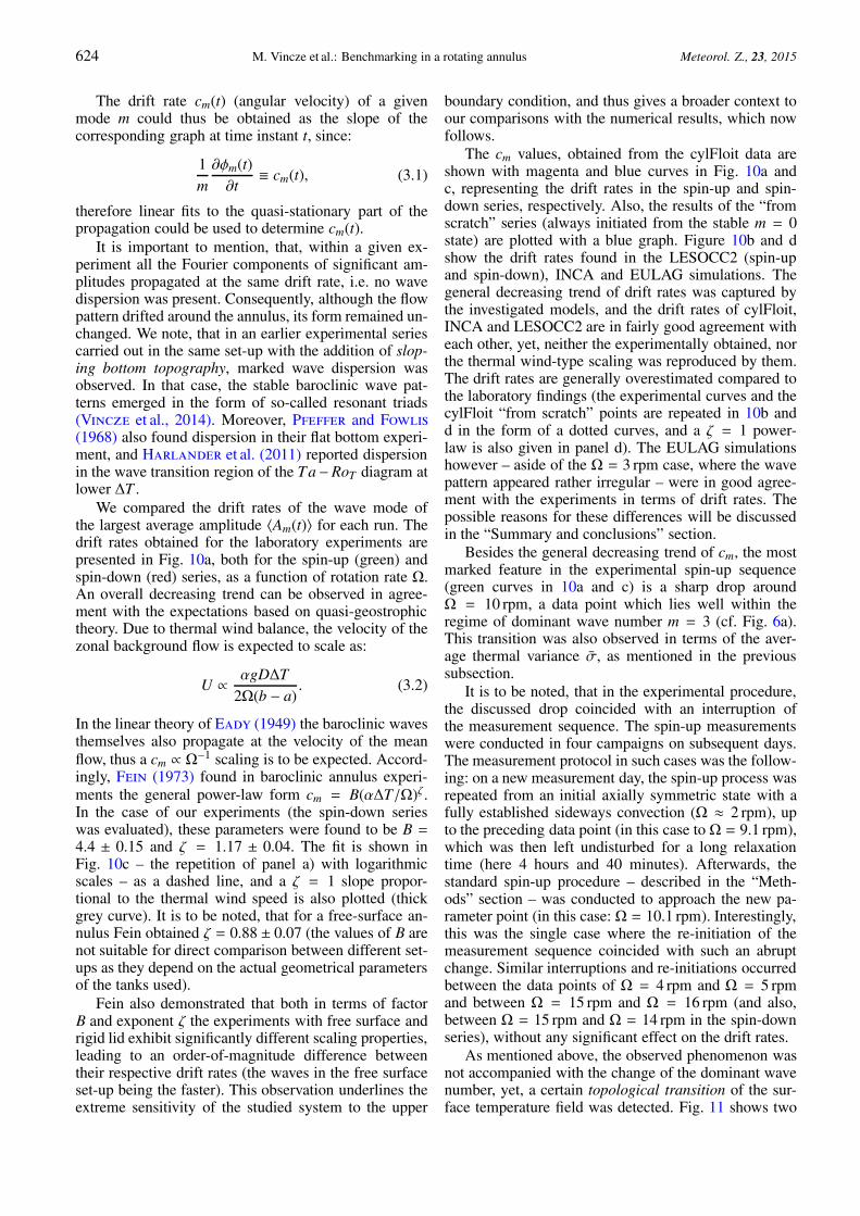
We compared the drift rates of the wave mode ofthe largest average amplitude 〈Am(t)〉 for each run. Thedrift rates obtained for the laboratory experiments arepresented in Fig. 10a, both for the spin-up (green) andspin-down (red) series, as a function of rotation rate Ω.An overall decreasing trend can be observed in agree-ment with the expectations based on quasi-geostrophictheory. Due to thermal wind balance, the velocity of thezonal background flow is expected to scale as:

U ∝ αgDΔT2Ω(b − a)

. (3.2)

In the linear theory of Eady (1949) the baroclinic wavesthemselves also propagate at the velocity of the meanflow, thus a cm ∝ Ω−1 scaling is to be expected. Accord-ingly, Fein (1973) found in baroclinic annulus experi-ments the general power-law form cm = B(αΔT/Ω)ζ .In the case of our experiments (the spin-down serieswas evaluated), these parameters were found to be B =4.4 ± 0.15 and ζ = 1.17 ± 0.04. The fit is shown inFig. 10c – the repetition of panel a) with logarithmicscales – as a dashed line, and a ζ = 1 slope propor-tional to the thermal wind speed is also plotted (thickgrey curve). It is to be noted, that for a free-surface an-nulus Fein obtained ζ = 0.88 ± 0.07 (the values of B arenot suitable for direct comparison between different set-ups as they depend on the actual geometrical parametersof the tanks used).

Fein also demonstrated that both in terms of factorB and exponent ζ the experiments with free surface andrigid lid exhibit significantly different scaling properties,leading to an order-of-magnitude difference betweentheir respective drift rates (the waves in the free surfaceset-up being the faster). This observation underlines theextreme sensitivity of the studied system to the upper

boundary condition, and thus gives a broader context toour comparisons with the numerical results, which nowfollows.

The cm values, obtained from the cylFloit data areshown with magenta and blue curves in Fig. 10a andc, representing the drift rates in the spin-up and spin-down series, respectively. Also, the results of the “fromscratch” series (always initiated from the stable m = 0state) are plotted with a blue graph. Figure 10b and dshow the drift rates found in the LESOCC2 (spin-upand spin-down), INCA and EULAG simulations. Thegeneral decreasing trend of drift rates was captured bythe investigated models, and the drift rates of cylFloit,INCA and LESOCC2 are in fairly good agreement witheach other, yet, neither the experimentally obtained, northe thermal wind-type scaling was reproduced by them.The drift rates are generally overestimated compared tothe laboratory findings (the experimental curves and thecylFloit “from scratch” points are repeated in 10b andd in the form of a dotted curves, and a ζ = 1 power-law is also given in panel d). The EULAG simulationshowever – aside of the Ω = 3 rpm case, where the wavepattern appeared rather irregular – were in good agree-ment with the experiments in terms of drift rates. Thepossible reasons for these differences will be discussedin the “Summary and conclusions” section.

Besides the general decreasing trend of cm, the mostmarked feature in the experimental spin-up sequence(green curves in 10a and c) is a sharp drop aroundΩ = 10 rpm, a data point which lies well within theregime of dominant wave number m = 3 (cf. Fig. 6a).This transition was also observed in terms of the aver-age thermal variance σ, as mentioned in the previoussubsection.

It is to be noted, that in the experimental procedure,the discussed drop coincided with an interruption ofthe measurement sequence. The spin-up measurementswere conducted in four campaigns on subsequent days.The measurement protocol in such cases was the follow-ing: on a new measurement day, the spin-up process wasrepeated from an initial axially symmetric state with afully established sideways convection (Ω ≈ 2 rpm), upto the preceding data point (in this case to Ω = 9.1 rpm),which was then left undisturbed for a long relaxationtime (here 4 hours and 40 minutes). Afterwards, thestandard spin-up procedure – described in the “Meth-ods” section – was conducted to approach the new pa-rameter point (in this case: Ω = 10.1 rpm). Interestingly,this was the single case where the re-initiation of themeasurement sequence coincided with such an abruptchange. Similar interruptions and re-initiations occurredbetween the data points of Ω = 4 rpm and Ω = 5 rpmand between Ω = 15 rpm and Ω = 16 rpm (and also,between Ω = 15 rpm and Ω = 14 rpm in the spin-downseries), without any significant effect on the drift rates.

As mentioned above, the observed phenomenon wasnot accompanied with the change of the dominant wavenumber, yet, a certain topological transition of the sur-face temperature field was detected. Fig. 11 shows two


Figure 10: Drift rates of the dominant wave modes as functions of rotation rate Ω. In panel (a), the experimental spin-up (green), spin-down(red) sequences are presented, alongside the spin-up (magenta), spin-down (blue) and “from scratch” (dark green) series. In panel (b) thedrift rates from other numerical models are shown. For a better comparison, three curves of panel (a) are repeated here with dotted lines,using their original color coding. The data from panels a) and b) are repeated with double logarithmic scales in panels c) and d). Thepower-law fit of the (spin-down) experimental data points (dashed line) and ζ = 1 curves (grey) obtained via thermal wind balance are alsoshown.

typical snapshots, transformed to polar coordinates. Thepattern characteristic to the first, “classic” type of m = 3waves (observed in the range of 7.1 rpm ≤ Ω ≤ 9.1 rpm)is presented in panel a), whereas the structure of theslowly propagating type (10.1 rpm ≤ Ω ≤ 15.9 rpm)is visible in panel b). One can observe, that the neigh-boring cold eddies that are separated by the meanderingwarm jet in case a), are connected by cold filaments incase b) (e.g. the one in the white rectangle). This impliesthat the widely used experimental classification of baro-clinic waves in a rotating annulus – that is based on thedominant wave number only – is rather incomplete: al-though the values of Ω and ΔT are within a regime thatis (given a certain initialization method, either spin-upor spin-down) characterized by a single dominant wavenumber m, yet, even within this regime, considerablejump-wise state transitions may occur (in terms of pat-tern topology and also in terms of drift rate) and clearlydifferent dynamical states may develop that essentiallyhave the same dominant zonal wave number.

Similarly to the experimental data, a pronouncedhysteresis appears at rotation rates Ω < 13 rpm in thecylFloit results (Fig. 10a). In this case the Ω-range ofthe hysteretic regime clearly agrees with the one foundin terms of the dominant wave numbers (cf. Fig. 6b).The interval between the intersection points of the spin-

up and spin-down curves (Ω = 6 rpm and Ω = 12 rpm)can therefore be described as the regime where m = 4is the dominant mode of the (lower) spin-down branchand the (upper) spin-down branch exhibits m = 3. Thus,a manifest correlation is present: at a given Ω the wavesof three-fold symmetry propagate faster than the four-fold-symmetric patterns. This conclusion is confirmedby the behavior observed in the from-scratch-initiatedsimulations of the dark green curve (see also the bluecurve of Fig. 6b): in the hysteretic regime, when thesystem switches from one branch to the other in termsof m, it does so in the drift rate as well. Note, that belowΩ = 10.1 rpm (where the aforementioned topologicalre-organization and sudden drop in the drift rates tookplace), also in the experimental data of Fig. 10a, theintersection point of the two branches coincides withthe onset of the m = 3 mode in the spin-up sequence,whereas the spin-down branch maintains the dominantwave number of m = 4. In other words: the “first” typeof m = 3 patterns (seen in Fig. 11a) drifts faster than thebaroclinic waves of m = 4 at a given rotation rate Ω.

3.4 Empirical Orthogonal Functions

To properly describe the temperature variance stored inco-existent spatio-temporal patterns in the annulus weturned to the method of Empirical Orthogonal Functions


Figure 11: Two thermographic experimental snapshots of m = 3 sur-face temperature patterns. A fastly propagating type (a), observed atrotation rate Ω = 4.2 rpm (see also the corresponding propagationplot in Fig. 9b), and (b) the slower type, observed after the “topolog-ical transition” (Ω = 10.1 rpm).

(EOFs) (Harlander et al., 2014). This approach is gen-erally accepted as a powerful tool for data compressionand dimensionality reduction: it is able to find the spa-tial patterns of variability, their time variation, and pro-vides a measure for the “relevance” of each pattern, andthus describe the complex behavior of the system, of-ten in terms of surprisingly few modes (Von Storchand Navarra, 1999). It is to be noted, however, thatin general these EOF modes do not necessarily corre-spond to individual dynamical eigenmodes of the system(Monahan et al., 2009).

EOF analysis has been extensively used in recentworks (Harlander et al., 2011; Borchert et al., 2014)for two-dimensional temperature and velocity fields inthe particular setup at BTU CS. Here, however, as werestricted our studies to the temperature profiles alongthe circular contour at mid-radius, the one-dimensionalEOFs were determined. Organizing the surface temper-ature data T (θ, t) at given time instants as column vec-tors (state vectors) and combining them in temporal or-der, yields the so-called data matrix X, whose number ofrows and columns correspond to that of the consideredspatial and temporal points, respectively. In the presentone-dimensional case a transparent visual representationof XT can be obtained in the form of a space-time orHovmöller plot, e.g. the one shown in Fig. 12a (corre-sponding to an m = 3 baroclinic wave).

In our EOF analyses the selected matrices X con-sisted of the data from the last 100 time instants of thegiven (either experimental or numerical) run; a time in-terval that always lied well within the quasi-stationarypart of the investigated process. In space, the experimen-

tal data were linearly interpolated onto an azimuthallyequidistant grid of 100 cells, whereas the numerical datawere transformed similarly to 50 grid points of uniformspacing. The entries of X were then obtained by sub-tracting the mean value of each corresponding row (i.e.temperature time series at a given spatial location). Thecovariance matrix S is given by:

S =1

n − 1XXT , (3.3)

where n = 100 is the number of time instants consid-ered. The eigenvectors ek (i.e. the EOFs themselves) andthe corresponding eigenvalues ξk of S were computed.The EOF index k = 1, 2, 3, . . . is given by organizing theeigenvalues in decreasing order as: ξ1 ≥ ξ2 ≥ ξ3 ≥ . . . .The percentage contribution pk of each pattern ek to thetotal variance captured by the EOFs can then be ex-pressed as: pk = ξk/

∑i ξi. As a demonstration, the first

four EOF patterns are shown in Fig. 12b, correspond-ing to the same experiment as the Hovmöller plot ofpanel a).

3.4.1 Variance distribution

The distribution of percentage contributions pk of theEOFs (a monotonically decreasing function of index k)was analyzed to quantify the overall complexity of theinvestigated spatio-temporal patterns. Typical “variabil-ity density functions” are presented in Fig. 13a, asobtained from our experiments (black, red and greencurves) and the simulations with different models (seealso the legend). It is to be emphasized that this figureserves a purely explanatory purpose: to help the readerto better understand the role of the parameters used toquantify the distribution properties. Therefore a largevariety of cases at different rotation rates are shown,which are therefore not meant for model comparison.Yet, some common features can be observed: visibly, ina large domain of k, the experimental data points exhibita power-law type scaling – indicating the importance ofhigher EOF indices – that is followed by exponentialcut-off. A qualitatively similar behavior can be observedin the numerical data as well, however, both the “power-law part” and the “cut-off part” appear to have differentquantitative properties than the ones of the experimentalresults.

To find appropriate measures of these properties,firstly the cumulative density functions I(k) =

∑ki=1 pk

were calculated for each experimental and numericalrun. Fig. 13b shows the I(k) curves corresponding to thecases plotted in panel a), with the same color coding.The heuristic empirical form

I(k) = 1 −Ce−αk

kβ(3.4)

has proven to be a strikingly accurate parametrizationfor every run: typically, the asymptotic standard errorswere below 3 % for all three free parameters α, β and C.


Figure 12: A typical thermografic Hovmöller (space-time) plot of an experimental run at dominant wavenumber m = 3 (a), and the firsttwo corresponding EOF variance pattern pairs (b and c). The corresponding relative variances of EOFs 1 to 4 were p1 = 0.29, p2 = 0.27,p3 = 0.082 and p4 = 0.073, respectively.

Figure 13: Typical variability density functions obtained from the experiments and numerical models (a). (See legends for the model typesand rotation rates). Their corresponding cumulative density functions are shown in panel (b) with the same color coding. The fitted parametervalues of α, β and C are also shown. Panels c) and d) show the density functions and cumulative density functions, respectively, for all themodels and the experiment for the Ω = 9 rpm (spin-up) case.

Note, that the values of these parameters for the exem-plary cases of Fig. 13b are listed in the legend. In pan-els c) and d) the density functions and cumulative den-sity functions of all the models (and the experiment) aregiven, all for a single parameter point Ω ≈ 9 rpm. For allmodels, the values of α, β and C were evaluated for eachsimulated Ω.

Let us now compare the fitted parameters β and αversus rotation rate Ω in Figs. 14a and b, respectively.In the laboratory experiments (red and green curvesin both panels) the values of β scatter in the range ofβ ∈ (0.3; 1.1), while α exhibits small positive valuesα ∈ (0.01; 0.1). These imply that the saturation of thecumulative density function is slow, a considerable part


Figure 14: The fitted parameters β and α of the cumulative densityfunctions of (3.4) versus rotation rate Ω: panels a) and b), respec-tively, and the correlation plot of the two parameters (c). The colorcoding is the same for all panels.

of the variance is stored in the EOFs of larger k. As theexponential factor is such a slowly varying function (dueto the small α), the behavior observed in the experimen-tal density functions of Fig. 13a approximately followsa power-law scaling in the form of k−γ ≡ k−β−1 with1.3 < γ < 2.1. Such values of γ are typical for the prob-ability density functions of long-range correlated pro-cesses. As yet another measure of complexity, it is to bementioned that k = 6 − 18 different EOFs were neededto cover 90 % (I(k) = 0.9) of the total variance in the ex-perimental distributions (like the first three graphs listedin Fig. 13b).

The exponent β was also typically found within thesame 0 < β < 1 regime in the simulations conducted byEULAG, HiFlow3 and LESOCC2 (see the black, grayand turquoise graphs in Figs.14a, respectively). Thisimplies that the distribution of variance in these threemodels behave realistically concerning the smaller k-regime, which practically corresponds to the large-scalefeatures of the flow. Also in terms of α, the EULAGresults scattered perfectly within the same interval asthe experiments, meaning that the “tail” of the distri-bution scales correctly. However, the values of param-eter C were an order of magnitude smaller for EULAG

(C ∈ (0.025; 0.12)) than for all the other cases, eitherexperimental or numerical, where C ∈ (0.42; 1.17) wasfound within the baroclinic unstable regime. This is dueto the interesting fact that in these simulations – despiteof their close-to-perfect scaling properties – the veryfirst EOF alone was responsible for 90–96 % of the to-tal variance, i.e. p1 ∈ (0.9; 0.96), a property that canbe observed on the turquoise curve of Fig. 13b too. ForHiFlow3 and LESOCC2, on the other hand, parameter αappeared to be 2–6 times larger than in the experiments(Fig. 14b), meaning that the variability of larger indicesk is suppressed by a marked exponential cut-off, thusmost of the variance is stored in the large-scale patterns.

The values of exponent beta were found significantlylarger in the INCA and cylFloit model runs than in thecase of the laboratory experiments (see orange, blue andmagenta graphs in Fig. 14a). Typically, the cases whereβ > 1 holds, correspond to α < 0, as visualized in thecorrelation plot of Fig. 14c. This relation suggests thatat smaller values of index k a sharp “fast” power lawcharacterizes the dominant, large-scale part of the distri-bution. This scaling, however, is confined only to thisregime: in itself it would mean a too sharp cut-off atlarger indices k. Thus, for an appropriate parametriza-tion, a negative value of α is needed to compensate thiseffect to keep the variances at higher EOF indices finite.

Regarding the cylFloit simulations the data points ofthe spin-up and spin-down series are plotted separately,with magenta and blue symbols in all panels of Fig. 14,respectively. In panel a) the marked hysteretic behaviorof parameter β can be observed. This behavior is inmanifest connection with the dominant wave numbers(cf. Fig. 6b): apparently, m = 4 states are characterizedby larger β than m = 3 states. This implies that in them = 4-dominated states the “scale separation” is morepronounced: a larger fraction of the total variance isstored in the first few EOF modes than in the m = 3cases.

In the spin-up and spin-down sequences of the lab-oratory experiments no such connection was found be-tween wave numbers and the parameters of I(k), how-ever, a significant jump of β at rotation rate Ω =10.1 rpm is visible in the spin-up curve (green graph inFig. 14a), that corresponds to the topological transitionwithin the m = 3 regime, described in the previous sec-tion.

3.4.2 Pattern correlations

Besides the distributions of the eigenvalues of covari-ance matrix S, the eigenvectors ek, i.e. the variancepatterns themselves were also compared. The appliedmethod was similar to the one used in Borchert et al.(2014) for two-dimensional EOFs. Firstly, the obtainedEOF patterns of indices k and l from the experimentand a given numerical model were linearly interpolatedonto the same equidistant grid of 100 cells. These func-tions are marked by: f exp

k (θ) and f modl (θ), respectively


(θ ∈ (0; 2π]). Their correlation coefficient is then calcu-lated as:

Ckl =〈 f exp

k (θ) f modl (θ + ϕ)〉 − 〈 f exp

k (θ)〉〈 f modl (θ + ϕ)〉

σ( f expk (θ))σ( f mod

l (θ + ϕ)),

(3.5)where 〈·〉 marks the azimuthal mean, σ(·) denotes thestandard deviation and ϕ is the “offset angle” whichmaximizes Ckl. This sliding transformation is required,since the azimuthal orientation of EOFs in the vari-ous models (and experimental runs) are generally differ-ent. In this transformation periodic boundary conditionswere applied, i.e. the values for which θ + ϕ > 2π wereactually mapped onto the interval (0;ϕ).

The values Ckl were calculated for the first 10 EOFs(both numerical and experimental) and were combinedinto 10 × 10 matrices. The structures of these matriceswere analyzed. Here, we present a few typical exem-plary cases to yield a qualitative insight to the natureof the correlation properties of one-dimensional EOFs.In Fig. 15 the correlation plots for the benchmark case#4 (Ω ≈ 17 rpm) are presented. This case was selected,since here – already out of the hysteretic regime – all themodels found m = 4 as dominant mode, in agreementwith the experiments. For a better understanding of thecomparisons to follow, in panel a) we present the corre-lation plot of the EOFs of the given experiment with oneanother (hence, f exp

i ≡ f modi using the above notation).

Trivially, in this case Cii = 1 holds for the diagonal en-tries, and the matrix is symmetric. Though the EOFs are,by definition, orthogonal, yet, the aforementioned slid-ing transformation leads to rather marked correlations,since EOF1 and EOF2 (and, similarly EOF3 and EOF4,etc.) are rather similar, but shifted in azimuthal direction(see also Fig. 12b and c). Such EOF pairs account for thebaroclinic wave propagation, analogously to the relationof sine and cosine terms in the Fourier decomposition ofpropagating waves.

Panels b)–f) show the correlation matrices obtainedfrom the comparison of the experimental set of EOFswith the EOFs from cylFloit, EULAG, HiFlow3, INCAand LESOCC2, respectively. The numbers on the hor-izontal axis represent the indices of the experimentalvariance patterns, and those on the vertical axis are theEOF indices of the given numerical model. The indicesand values of the maximum entries in the given ma-trix are also marked in the panels. Two main observa-tions need to be emphasized. Firstly, the structures ofthe matrices are rather similar, implying that the numer-ical models produce similar variance patterns. Also, theaforementioned EOF pairs are clearly visible in the ma-trices in the form of 2×1 and 2×2 blocks of closely simi-lar correlations. The second main observation is that, de-spite of the similarity of the matrices, none of them hasdiagonal structure as in panel a). Thus, the various EOFpatterns are ranked differently.

The latter statement is seemingly in contrast with thefindings of Borchert et al. (2014), who found correla-tion coeffitiens above 0.9 by comparing their EOFs (ob-

tained using the cylFloit and INCA codes) to the lab-oratory EOFs of the same index. However, there thefull two-dimensional surface temperature patterns weretaken. As a test of consistency, we applied our method-ology to the very same experimental records from year2011 and the same (“from-scratch” initiated) cylFloitruns studied in Borchert et al. (2014) to obtain the cor-relation coefficients for the one-dimensional EOFs. Theresulting correlation matrix is shown in Fig. 16a. Ap-parently, the obtained structure is quite similar to thoseseen in Fig. 15b-f, and lacks large values in the diagonal.However, the entries in the 2 × 2 blocks in he vicinity ofthe diagonal at lower left are indeed large, with a maxi-mum of C31 = 0.97. The similarities and differences ofthese patterns can be visually evaluated in Fig. 16b andc, where EOFs 1 and 3 are plotted for the experimentaland the numerical case, respectively. One can see, thatin the experimental case EOF1 exhibits wave numberm = 6 (and so does its shifted pair EOF2, not shownhere) and the dominant baroclinic wave number m = 3appears in the EOF3 for the first time, in contrast to thetypical numerical results. Thus, the numerical modelshave a tendency to underestimate the variance stored inthe smaller scales.

It can be stated that the one-dimensional data ex-tracted from the surface temperature field at mid-radiusrmid are generally more sensitive to smaller-scale dif-ferences than the full two-dimensional patterns, since –as discussed above – in the two-dimensional case nosuch “EOF swap” occurs between numerics and exper-iment. The mid-radius temperature profiles are appar-ently largely effected by the variance stored in the har-monics of the dominant baroclinic wave mode, relatedto the structure and dynamics of the cold eddies in thelobes of baroclinic waves. The fact that the numericalmodels are apparently not able to resolve these phenom-ena implies that they may well be related to boundarylayer effects or even “wind” stress above the free sur-face of the laboratory tank, which are clearly out of thescope of the investigated numerical models.

Also, it is to be noted, that in an annulus with an exactrotational invariance the EOFs must be sinusoidal, i.e.each would project on a single azimuthal wave numberonly, as shown by Achatz and Schmitz (1997). Thefact that the typical EOFs of the experiment can in manycases visibly be decomposed to at least two wave num-bers (as the ones in Fig. 12b and Fig. 16b) indicates aviolation of rotational symmetry and nonlinear dynam-ics. In the azimuthally invariant numerical models (ascylFloit), however, the EOF patterns were indeed foundto be nearly sinusoidal (see e.g. Fig. 16c). Their slightimperfection is merely a consequence of the finite lengthof the time series considered.

4 Summary and conclusions

In this work we have critically compared various exper-imentally and numerically obtained characteristic prop-erties of baroclinic instability in a differentially heated


Figure 15: The cross-correlation matrices obtained in the benchmark case #4 (Ω ≈ 17 rpm). The positions and values of the maximumentries of the matrices are also given underneath the respective figures.

Figure 16: The correlation matrix of the one-dimensional EOFs, obtained from the numerical and experimental data of test case #7 ofBorchert et al. (2014), and the value of the maximum entry (a). EOFs 1 and 3 of the experimental (a) and numerical (b) case. Note the“swap” between the indices and wave patterns of the two cases.

rotating annulus. Our systematic comparison of fivedifferent numerical models to laboratory experiments(“benchmarking”) was largely motivated by the generalneed to validate numerical models and procedures to beused for modeling large-scale atmospheric flows.

Two series of laboratory measurements were per-formed: the “spin-up” and “spin-down” sequences. Be-tween each measurement only rotation rate Ω was ad-justed, while the radial temperature difference ΔT ≈8 K remained constant. The two sequences enabled us

to scan through the investigated parameter range withdifferent initial conditions, and thus access multipleequilibrium regimes. In agreement with earlier results(Miller and Butler, 1991; Sitte and Egbers, 2000;Von Larcher et al., 2005) a considerable hysteresis wasfound in terms of the dominant azimuthal wave numbersm of the baroclinic waves.

It is well established since the works of James et al.(1981) and Hignett et al. (1985) in the 1980s, that interms of m, the development of baroclinic waves in baro-


clinic annuli can be captured in direct numerical simula-tions fairly well. In the present work we also found thatm is indeed a robust indicator of the flow state, and itsobtained values exhibit good agreement between the ex-periments and the numerical runs. The numerical resultsalso support our conclusion that the hysteretic behav-ior of m is to be interpreted as distinct multiple equilib-ria and is not just caused by transient phenomena. Thisstatement is backed by the following observations: (i)Simulation series conducted with models cylFloit andLESOCC2 imitated the “spin-up” and “spin-down” se-quences and found hysteresis in terms of m. A thirdbunch of simulations, however, were always initializedfrom the axially symmetric stable state (cylFloit “fromscratch” sequence). Yet, occasionally even here, wavenumbers characteristic to the “spin-down” branch werefound to develop within a rotation rate regime wherethese simulations typically converged to the states ofthe “spin-up” branch. (ii) In the HiFlow3 simulations,runs with slightly perturbed initial conditions were alsoconducted. The only cases where these temperature dis-turbances yielded a different dominant wave number mthan that corresponding to the unperturbed runs wereat parameter points within the experimentally observedhysteretic Ω-regime.

The different routes of releasing the stored poten-tial energy – as initial conditions – may play impor-tant roles in the observed hysteretic mode (i.e. dominantm-) selection. If spin-up is applied, the inclination ofthe iso-density surfaces increases, making the flow more“baroclinic unstable”, i.e. the stored potential energy istransformed into kinetic energy only via enhanced baro-clinic wave excitation (a very effective way of energy re-lease). If spin-down is applied, the inclination of isopyc-nals decrease, and the unavoidable transient hydrostaticimbalance opens up the way to other forms of kineticenergy release as well, via the overturning backgroundflow (possibly even inertia-gravity wave excitation, seee.g. the numerical work of Randriamampianina et al.(2006)). Although these effects are probably transient,yet, as initial conditions they appear to play an importantrole in setting the dominant wave number m of the baro-clinic wave, which remains steady for a much longertime than the timescale characteristic for the reorgani-zation of stratification.

Another important measure of baroclinic wave dy-namics is the drift rate cm of the dominant wave mode.In qualitative agreement with the quasigeostrophic Eadymodel (Vallis, 2006), the cm(Ω) relationship was foundto be a decreasing function, roughly following thecm ∝ Ω−1 dependence set by the thermal wind bal-ance. It is to be noted, however, that most of the mod-els (with the exception of EULAG) systematically over-estimated the wave speeds. This phenomenon may wellbe explained by the simulations’ difficulties to resolvethe boundary layer drag at the lateral sidewalls. A simi-lar observation was described in the study of Williamset al. (2010) where a two-layer (lid shear-driven) rotat-ing baroclinic annulus set-up was investigated both ex-

perimentally and numerically. In their case the simu-lated drift rates were larger than the measured valuesby a factor of 4, due to the model’s neglect of Stew-artson layer drag. Stewartson layers are characteristicfor homogeneous fluids. In our case of relatively strongstratification, however, Pr RoT /Γ

2 � Ek2/3 holds withΓ being the vertical aspect ratio of the tank (as definedin Section 2) and Ek = ν/(ΩL2) the Ekman number.In this regime – instead of Stewartson layers – twoboundary layers are found in the vicinity of each lateralsidewall: the larger hydrostatic layer with a character-istic thickness of δh = D(Pr RoT/Γ

2)1/2 and, closer tothe wall, the buoyancy layer whose thickness is δb =

D(νκ/(D3gαΔT ))1/4. These two layers unite and formthe Stewartson layer (with δS = D Ek1/3) if stratifica-tion decreases (Barcilon and Pedlosky, 1967). Forthe present case δh > b − a holds, i.e. practically thewhole measurement cavity lies within the “hydrostatic”domain. The buoyancy layer, however, is found to beonly δb ≈ 1 mm thick, thus it is not resolved sufficientlyby most of the models.

The sensitivity of drift rates to the horizontal gridspacing was demonstrated with the INCA model. Thephase speeds of baroclinic waves at two different ro-tation rates – namely Ω = 4 rpm and Ω = 9.5 rpm –were determined using two grids in both cases for com-parison. The coarse and fine grids had minimum cellsizes of Δxmin,(1) = Δymin,(1) = 1.5 mm and Δxmin,(2) =Δymin,(2) = 0.5 mm, respectively. The obtained drift rateswere: c(1) = 0.097 rad/s (coarse grid); c(2) = 0.057 rad/s(fine grid) at Ω = 4 rpm, and c(1) = 0.025 rad/s (coarsegrid); c(2) = 0.023 rad/s (fine grid) at Ω = 9.5 rpm. Vis-ibly, at the lower rotation rate (where the phase veloci-ties of baroclinic waves are generally large) the refine-ment of the horizontal grid yielded slower wave prop-agation almost by a factor of two. In the case of thehigher rotation rate this effect was manifestly smaller –around 10 % – in qualitative agreement with the drag-hypothesis: the drag itself is expected to be smaller tooif the drift itself is slower. Thus, we can conclude that thegrid resolution has marked effect on the simulated wavespeeds, and to get a proper insight into the flow structureat the vicinity of the lateral sidewalls, one needs to applygrids that properly resolve the buoyancy layer.

We also found marked connection between the spa-tial patterns of baroclinic waves and their drift rates,both experimentally and numerically. The aforemen-tioned hysteresis that was observed in terms of the domi-nant wave number m also manifested itself in the driftrates. In the cylFloit simulations, m = 3 waves al-ways propagated faster than their m = 4 counterpartsat a given rotation rate (within the hysteretic Ω-regime).Similar behavior was noticed in the laboratory experi-ments too: a certain type of the m = 3 wave was found tobe faster than the m = 4 waves of the same Ω. However,in the laboratory, another type of three-fold symmetric(m = 3) pattern appeared as well in the “spin-up” series,which was found to propagate at an even smaller speed


than the m = 4 waves. Here the surface temperature pat-tern has undergone a “topological” reorganization: themeandering warm jet that separated the inner and outerdomain in the “fast” m = 3 waves has disconnected.This transition possibly opens the way for stronger ra-dial temperature fluxes, therefore this new configurationmay reduce the thermal wind (background flow) moreeffectively, yielding slower drift. Applying the same rea-soning for the hysteresis of m = 4 waves and the “fast”m = 3 waves, it can be stated that among these, them = 4 mode exhibits larger radial heat flow. As far asthe general heat flow is considered, Rayer et al. (1998)showed that the Nusselt number Nu in a baroclinic an-nulus exhibits a large drop at the transition from ax-isymmetric flow to the regime of regular waves, where –compared to the abrupt change at the onset of baroclinicinstability – it does not change markedly with the in-creasing Ω. This plateau of Nu(Ω) is followed by an-other pronounced drop of Nu when the system reacheshigher rotation rates where the waves become irregular(this state was not studied in the present work). It is tobe noted, that the changes in heat flow that can be at-tributed to shape changes of regular baroclinic wavesis rather small compared to the aforementioned changesbetween the general flow states. We also remark, that –as demonstrated in the experiments of Fein (1973) – thedrift rates are also highly sensitive to the upper boundarycondition, that was not prescribed properly in the modelequations.

The third main focus of our study was the statisticalquantification of the structures of the surface tempera-ture field and the analysis of their spatio-temporal vari-ability. As a measure of the overall variability in the sys-tem, the time averaged temperature variance σ(Ω) takenalong the circular contour at mid radius rmid served asan order parameter that indicates the breaking of the ax-ial symmetry (and, thus, the onset of baroclinic instabil-ity) with a marked jump at critical rotation rate Ωcrit. In-deed, in the numerical simulations σ ≈ 0 was detected inall cases where no dominant wave mode could be found(aside for the trivial m = 0), implying the stability of theaxially symmetric basic state. This was then followed bymore than 10 times larger variances at Ω > Ωcrit. How-ever, in the laboratory experiments the transition was notthat apparent: even below Ωcrit fluctuations appeared onthe same order of magnitude as the σ values of higherrotation rates (though, smaller by a factor of around 0.5).This observation confirms our previous finding of spon-taneous excitation of dispersive transient wave-like phe-nomena (coined “weak waves”) that “blur” the bound-ary of instability in the parameter space (Vincze et al.,2014). This qualitative difference between numerics andexperiments indicates the presence of non-modal tran-sient growth of small temperature fluctuations in thissensitive regime (Seelig et al., 2012) unavoidable in thelaboratory (see also the work of Hoff et al. (2014) inthe present volume). In the numerical results the tem-perature variance obtained at a few centimeters belowthe surface was found to be significantly larger (by a

factor of around 2) than at the surface. This behavior,however, could not be verified experimentally with theapplied measurement techniques.

In order to analyze smaller scale spatial structures,we calculated the Fourier spectra of the azimuthal tem-perature profiles along the circular contour at mid-radiusrmid for all time instants of a given experimental ornumerical run, and their temporal average was consid-ered as the characteristic spectral “fingerprint” of theinvestigated pattern. In the case of an m-fold symmet-ric baroclinic wave, besides the dominant wave num-ber, its harmonics also appear in the spectra with fi-nite amplitudes, as already demonstrated by James et al.(1981). The amplitudes and the significance of the spec-tral peaks provide a measure of the importance of theregular smaller scale patterns. Typically, in the exper-imental data marked amplitudes were observed at theinteger multiples of the dominant mode. These ampli-tudes were, in many cases, comparably large to that ofthe dominant wave number (representing the overall ro-tational symmetry). In the cylFloit simulations however,the harmonics were not that pronounced. These smaller-scale patterns are attributed to the cold eddies outsideand inside the meandering jet of the baroclinic wave.The fact that these structures could not be resolved accu-rately in the simulations may be due to the following rea-sons: the cold eddies in the vicinity of the outer rim seemto be excited by shear instability involving the bouyancylayer, which was not resolved by most of the models,as discussed above. This statement is supported by theobservation that the high-resolution EULAG tempera-ture fields occasionally showed such structures (cf. vonLarcher and Dörnbrack (2014) in the present issue).Surface phenomena that are out of the scope of the stud-ied governing equations may also contribute to makingthese cold eddies more pronounced. Such factors can bee.g. the “wind” stress that takes place at the free sur-face of the experimental tank as it rotates, or the pres-ence of finite vertical heat fluxes at the top surface (note,that all the models included the ∇T �ez|z=D = 0 typeno-flux boundary conditions, which certainly cannot beachieved in the experiment due to the free surface). Therole of the slight curvature of the top surface due to thecentrifugal effect is probably negligible: the water depthdifference Δd between the inner and outer rim is foundto be Δd = Ω2(b2 − a2)/(2g) ≈ 0.4 − 2.5 mm in the ap-plied rotation rate regime. Nevertheless, this minor geo-metric distortion also adds to the list of effects that werenot implemented in the numerical models.

The azimuthal temperature variance patterns weredecomposed into sets of empirical orthogonal functions(EOFs). We found that in the experimental distribu-tion of the ranked relative variances – the normalizedeigenvalues corresponding to the EOF modes – typi-cally follows a slowly decaying power-law type scaling,implying that a considerable part of the total varianceis stored in the smaller scales (6–18 orthogonal modeswere needed to cover 90 % of the total variance). Ingeneral, the numerically obtained distributions exhibited


faster cut-offs towards the higher ranks, thus less small-scale variance. The practical absence of the correlatedsmall-scale thermal fluctuations in the simulations sup-ports the need for some subgrid-scale parametrizationthat takes into account the growth of temperature fluc-tuations that might play a significant role in the dynam-ics. These fluctuations can be caused by the aforemen-tioned experimental impurities (or possibly induced byboundary layer effects) and “inflated” through the non-linear interactions. Since the present work (and the Met-Ström collaboration in general) has been motivated bymeteorological problems, it is important to emphasize,that obviously, the sub-grid-scale processes of the atmo-sphere are very different from, and way more complexthan, those of our experimental set-up. Yet, our observa-tions of how the small-scale variability affects the stabil-ity of the larger-scale patterns in the set-up – regardlessof the actual physical processes at subgrid-scales – froma more general, dynamical systems point of view, mayalso be of relevance for atmospheric or oceanic model-ing.

Due to the differences between the numerical proce-dures, drawing general summarizing conclusions fromthe present study is far from straightforward. Thecodes built by the numerical groups of our collabo-ration were all developed based on the already exist-ing solvers and numerical schemes that the respectivegroups have previously gained experience with, inde-pendently from modeling the differentially heated ro-tating annulus. Therefore, since the models were dif-ferent in so many aspects (reference frames, grid struc-tures, resolutions, subgrid-scale parametrizations, etc.),the “parameter space” of model features was so large,that no benchmarking strategy could have been inten-tionally defined for comparing models of increasing de-grees of complexity from one single aspect.

However, the main message of our results is that de-spite of all this large diversity of the applied codes, theydo share some interesting commonalities. Firstly, theexperimentally obtained dominant wave numbers werefairly well reproduced by all the codes. This is some-what surprising in the light of the fact that the drift rates(that are closely related to strength of the zonal back-ground flow) were systematically overestimated by allthe models, except EULAG. This latter common featurewas found to be the consequence of improper grid res-olution at the vicinity of the vertical sidewalls, wherethe boundary layer drag was not sufficiently resolved.As another general “message to take home” we can alsostate that (i) the small-scale variability was not capturedproperly by the models, as discussed above, yet (ii), thelarge-scale patterns are properly reproduced. Thus, de-spite of the obvious nonlinearity of the studied dynam-ics, we can state that the coupling (‘information trans-fer’) between the smaller and larger scales does not playsuch a critical role in the studied flow regimes.

As a possible extension and continuation of this idea,the response of the system to small amplitude temporaland spatial thermal fluctuations (entering via the bound-

ary conditions) could be analyzed numerically in a fu-ture research project. Such investigations – if the aboveassumptions are correct – can possibly lead to evenmore accurate numerical modeling and a deeper under-standing of the dynamics in this set-up. Also, our futureplans involve the extension of the presented benchmark-ing techniques to numerical methods that reach beyondthe Boussinesq approximation (e.g. Low-Mach models)whose application may be wise in the larger ΔT -regime.

The results presented in this paper have clearlydemonstrated that the relatively simple rotating annu-lus arrangement indeed provides a remarkable test bedto verify and tune numerical methods aiming to modellarge-scale atmospheric flows. The authors think that thepresented pool of experimental and numerical data andthe applied evaluation methods and “test quantities” willalso prove useful benchmarks for similar studies in thefuture.

AcknowledgementsThis work has been funded by the German ScienceFoundation (DFG) and is part of the DFG priority pro-gram MetStröm (SPP 1276, EG 100/13-1 to 13–3). Theexperimental team (U.H., M.V., K.A. and C.E.) is grate-ful for the technical help of H.-J. Pflanz, R. Stöbeland Y. Wang throughout the period of the whole Met-Ström program. The work of U.H., M.V. and Th. v. L.was partially supported by DAAD-PROCOPE grant55908227 ‘Baroclinic waves’. The Hiflow3 team (M.B.,T.B. and V.H.) gratefully acknowledges the computingtime granted by the John von Neumann Institute forComputing (NIC) and provided on the supercomputerJUROPA at Jülich Supercomputing Centre (JSC). Thework of the HiFlow3 team was partially supported bygrant HE4760/3-3 (DFG). The cylFloit team (S.B. andU.A.) were also financed through DFG grant Ac71/4-2.The INCA team (S.R. and S.H.) was supported by DFGgrant HI1273-1, and the computational resources wereprovided by the HLRS Stuttgart, under grant TIGRA.The EULAG numerical data were generated using re-sources of the Department of Mathematics and Com-puter Science, Freie Universität Berlin, Germany. Com-puting time for the results obtained with LESOCC2(C.H. and J.F.) was provided by ZIH at TU Dresden.M.V. acknowledges the discussions with the members ofthe project group “Physical Mechanisms of Global Envi-ronmental Processes” (Budapest, Hungary, Grant num-ber NK100296). We are also very grateful to guest editorDieter Etling and the two anonymous referees for theirhighly insightful remarks. We are also very grateful toguest editor Dieter Etling, the two anonymous referees,and Fred Feudel for their highly useful remarks.

ReferencesAchatz, U., G. Schmitz, 1997: On the closure problem in the

reduction of complex atmospheric models by PIPs and EOFs:A comparison for the case of a two-layer model with zonallysymmetric forcing. – J. Atmos. Sci. 54, 2452–2474.


Barcilon, V., J. Pedlosky, 1967: A unified linear theory ofhomogeneous and stratified rotating fluids. – J. Fluid Mech.29, 609–621.

Borchert, S., U. Achatz, S. Remmler, S. Hickel, U. Har-lander, M. Vincze, K.D. Alexandrov, F. Rieper, T. Hep-pelmann, S.I. Dolaptchiev, 2014: Finite-volume modelswith implicit subgrid-scale parameterization for the differen-tially heated rotating annulus. – Meterol. Z. 23, this issue.

Brezzi, F., 1974: On the existence, uniqueness, and approx-imation of saddle point problems arising from Lagrangianmultipliers. – Revue française d’automatique, informatique,recherche opérationnelle. Analyse Numérique 8, 129–151.

Chorin, A.J., 1968: Numerical solution of the Navier–Stokesequations. – Math. Comp. 22, 745–762.

Cotter, C., P. Smolarkiewicz, I. Szczyrba, 2002: A visco-elastic fluid model for brain injuries. – Int. J. Num. Meth.Fluids 40, 303–311.

Eady, E., 1949: Long waves and cyclone waves. – Tellus 1,33–52.

Elliott, J., P. Smolarkiewicz, 2002: Eddy resolving simula-tions of turbulent solar convection. – Int. J. Num. Meth. Fluids39, 855–864.

Fein, J.S., 1973: An experimental study of the effects of theupper boundary condition on the thermal convection in arotating, differentially heated cylindrical annulus of water. –Geophys. Astrophys. Fluid Dyn. 5, 213–248.

Fröhlich, J., 2006: Large Eddy Simulation turbulenter Strö-mungen – Teubner Verlag, 414 pp.

Früh, W.-G., P. Read, 1997: Wave interactions and the transitionto chaos of baroclinic waves in a thermally driven rotatingannulus. – Philosophical Transactions of the Royal Society ofLondon. Series A: Math. Phys. Engin. Sci. 355, 101–153.

Fultz, D., R.R. Long, G.V. Owens, J. Weil, 1959: Studies ofthermal convection in a rotating cylinder with some implica-tions for large-scale atmospheric motions – American Meteo-rological Society, Meteorological monographs, v. 4, no. 21.

Goldstein, D., R. Handler, L. Sirovich, 1993: Modeling a no-slip flow boundary with an external force field. – J. Comput.Phys. 105, 354–366.

Grabowski, W., P. Smolarkiewicz, 2002: A multiscale anelas-tic model for meteorological research. – Mon. Wea. Rev. 130,939–956.

Grilli, M., P.J. Schmid, S. Hickel, N.A. Adams, 2012: Analy-sis of unsteady behaviour in shockwave turbulent boundarylayer interaction. – J. Fluid Mech. 700, 16–28.

Gyüre, B., I. Bartos, I.M. Jánosi, 2007: Nonlinear statisticsof daily temperature fluctuations reproduced in a laboratoryexperiment. – Phys. Rev. E 76, 037301.

Harlander, U., R. Faulwetter, K. Alexandrov, C. Egbers,2009: Estimating local instabilities for irregular flows in thedifferentially heated rotating annulus. – In: Advances in Tur-bulence XII, Springer, 163–166.

Harlander, U., T. von Larcher, Y. Wang, C. Egbers, 2011:PIV and LDV measurements of baroclinic wave interactions ina thermally driven rotating annulus. – Exp. Fluids 51, 37–49.

Harlander, U., J. Wenzel, K. Alexandrov, Y. Wang, C. Eg-bers, 2012: Simultaneous PIV and thermography measure-ments of partially blocked flow in a differentially heated ro-tating annulus. – Exp. Fluids 52, 1077–1087.

Harlander, U., T. von Larcher, G.B. Wright, M. Hoff,K.D. Alexandrov, C. Egbers, 2014: Orthogonal decom-position methods to analyze PIV, LDV and thermogra-phy data of a thermally driven rotating annulus labora-tory experiment. – In: T. von Larcher, P.D. Williams (eds.):Modelling Atmospheric and Oceanic flows: Insight fromLaboratory Experiments and Numerical Simulations. Wiley,DOI: 10.1002/9781118856024.ch17

Heuveline, V., 2010: HiFlow3: A flexible and hardware-awareparallel finite element package. – In: Proceedings of the9th Workshop on Parallel/High-Performance Object-OrientedScientific Computing, POOSC ’10, 4:1–4:6, New York, NY,USA. ACM.

Heuveline, V., E. Ketelaer, S. Ronnas, M. Schmidto-breick, M. Wlotzka, 2012: Scalability study of HiFlow3based on a fluid flow channel benchmark. – EMCL PreprintSeries (2012/1).

Hickel, S., N.A. Adams, J.A. Domaradzki, 2006: An adaptivelocal deconvolution method for implicit LES. – J. Comput.Phys. 213, 413–436.

Hickel, S., T. Kempe, N.A. Adams, 2008: Implicit large-eddysimulation applied to turbulent channel flow with periodicconstrictions. – Theo. Comput. Fluid Dyn. 22, 227–242.

Hignett, B.P., A. White, R. Carter, W. Jackson, R. Small,1985: A comparison of laboratory measurements and numeri-cal simulations of baroclinic wave flows in a rotating cylindri-cal annulus. – Quart. J. Roy. Meteor. Soc. 111, 131–154.

Hinterberger, C., J. Fröhlich, W. Rodi, 2007: Three-dimensional and depth-averaged large-eddy simulations ofsome shallow water flows. – J. Hydraulic Engin. 133,857–872.

Hoff, M., U. Harlander, C. Egbers, 2014: Empirical singularvectors of baroclinic flows deduced from experimental dataof a differentially heated rotating annulus. – Meteorol. Z. 23,581–597, DOI: 10.1127/metz/2014/0563

James, I., P. Jonas, L. Farnell, 1981: A combined labora-tory and numerical study of fully developed steady baroclinicwaves in a cylindrical annulus. – Quart. J. Roy. Meteor. Soc.107, 51–78.

Jánosi, I.M., P. Kiss, V. Homonnai, M. Pattantyús-Ábrahám, B. Gyüre, T. Tél, 2010: Dynamics of passive trac-ers in the atmosphere: Laboratory experiments and numericaltests with reanalysis wind fields. – Phys. Rev. E 82, 046308.

Lorenz, E.N., 1963: The mechanics of vacillation. – J. Atmos.Sci. 20, 448–465.

Mason, P., 1975: Baroclinic waves in a container with slopingend walls. – Philosophical Transactions of the Royal Societyof London. Series A, Math. Phys. Sci. 278, 397–445.

Mayer, J., 2007: Ilu++: A new software package for solvingsparse linear systems with iterative methods. – PAMM 7,2020123–2020124.

Meyer, M., S. Hickel, N. Adams, 2010: Assessment of implicitlarge-eddy simulation with a conservative immersed interfacemethod for turbulent cylinder flow. – Int. J. Heat Fluid Flow31, 368–377.

Miller, T.L., K.A. Butler, 1991: Hysteresis and the transitionbetween axisymmetric flow and wave flow in the baroclinicannulus. – J. Atmos. Sci. 48, 811–824.

Monahan, A.H., J.C. Fyfe, M.H. Ambaum, D.B. Stephen-son, G.R. North, 2009: Empirical orthogonal functions: Themedium is the message. – J. Climate 22, 6501–6514.

Pfeffer, R.L., W.W. Fowlis, 1968: Wave dispersion in a rotat-ing, differentially heated cylindrical annulus of fluid. – J. At-mos. Sci. 25, 361–371.

Prusa, J., P. Smolarkiewicz, A. Wyszogrodzki, 2008: EU-LAG, a computational model for multiscale flows. – Comput-ers &Fluids 37, 1193–1207.

Randriamampianina, A., W.-G. Früh, P.L. Read,P. Maubert, 2006: Direct numerical simulations of bi-furcations in an air-filled rotating baroclinic annulus. –J. Fluid Mech. 561, 359–389.

Ravela, S., J. Marshall, C. Hill, A. Wong, S. Stransky,2010: A realtime observatory for laboratory simulation ofplanetary flows. – Experiments in Fluids 48, 915–925.

http://dx.doi.org/10.1002/9781118856024.ch17

http://dx.doi.org/10.1127/metz/2014/0563


Rayer, Q., D. Johnson, R. Hide, 1998: Thermal convection in arotating fluid annulus blocked by a radial barrier. – Geophys.Astrophys. Fluid Dyn. 87(3-4), 215–252.

Read, P.L., 2003: A combined laboratory and numerical study ofheat transport by baroclinic eddies and axisymmetric flows. –J. Fluid Mech. 489, 301–323.

Read, P., S. Lewis, R. Hide, 1997: Laboratory and numericalstudies of baroclinic waves in an internally heated rotatingfluid annulus: a case of wave/vortex duality?. – J. Fluid Mech.337, 155–191.

Read, P.L., P. Maubert, A. Randriamampianina, W.-G. Früh,2008: Direct numerical simulation of transitions towardsstructural vacillation in an air-filled, rotating, baroclinic an-nulus. – Phys. Fluids (1994-present) 20, 044107.

Remmler, S., S. Hickel, 2012: Direct and large eddy simulationof stratified turbulence. – Int. J. Heat Fluid Flow 35, 13–24.

Remmler, S., S. Hickel, 2013: Spectral structure of strati-fied turbulence: Direct numerical simulations and predictionsby large eddy simulation. – Theo. Comput. Fluid Dyn. 27,319–336.

Rhie, C.M., W.L. Chow, 1983: Numerical study of the turbulentflow past an airfoil with trailing edge separation. – AIAA J.21, 1525–1532.

Schröttle, J., A. Dörnbrack, 2013: Turbulence structurein a diabatically heated forest canopy composed of fractalpythagoras trees. – Theo. Comput. Fluid Dyn. 27, 337–359.

Seelig, T., U. Harlander, R. Faulwetter, C. Egbers, 2012:Irregularity and singular vector growth in the differentiallyheated rotating annulus. – Theo. Comp. Fluid Dyn. 27,415–432

Shu, C.-W., 1988: Total-variation-diminishing time discretiza-tions. – SIAM Journal of Scientific and Statistical Computing9, 1073–1084.

Sitte, B., C. Egbers, 2000: Higher order dynamics of baroclinicwaves. – In: Physics of Rotating Fluids, Springer, 355–375.

Smolarkiewicz, P., 1991: On forward-in-time differencing forfluids. – Monthly Weather Review 119, 2505–2510.

Smolarkiewicz, P., L. Margolin, 1997: On forward-in-timedifferencing for fluids: An eulerian/semi-lagrangian nonhy-drostatic model for stratified flows. – Atmos.-Ocean Special35, 127–157.

Smolarkiewicz, P., L. Margolin, 1998: MPDATA: A positivedefinite solver for geophysical flows. – J. Comput. Phys. 140,459–480.

Smolarkiewicz, P., R. Sharman, J. Weil, S. Perry, D. Heist,G. Bowker, 2007: Building resolving large-eddy simulationsand comparison with wind tunnel experiments. – J. Comput.Phys. 227, 633–653.

Vallis, G.K., 2006: Atmospheric and oceanic fluid dynamics:fundamentals and large-scale circulation. – Cambridge Uni-versity Press.

Vettin, F., 1857: Über den aufsteigenden Luftstrom, die Entste-hung des Hagels und der Wirbel-Stürme. – Ann. Phys. Chem.102, 246–255.

Vincze, M., U. Harlander, T. von Larcher, C. Egbers, 2014:An experimental study of regime transitions in a differen-tially heated baroclinic annulus with flat and sloping bottomtopographies. – Nonlinear Proc. Geoph. 21, 237–250.

Von Larcher, T., A. Dörnbrack, 2014: Numerical simulationsof baroclinic driven flows in a thermally driven rotating annu-lus using the immersed boundary method. – Meteorol. Z. 23,599–610, DOI: 10.1127/metz/2014/0609

Von Larcher, T., C. Egbers, 2005: Experiments on transitionsof baroclinic waves in a differentially heated rotating annu-lus. – Nonlinear Proc. Geoph. 12, 1033–1041.

Von Larcher, T., A. Fournier, R. Hollerbach, 2013: Theinfluence of a sloping bottom endwall on the linear stability inthe thermally driven baroclinic annulus with a free surface. –Theo. Comput. Fluid Dyn. 27), 433–451.

von Storch, H., A. Navarra, 1999: Analysis of climatevariability: applications of statistical techniques. – Springer,342 pp.

Williams, G.P., 1971: Baroclinic annulus waves. – J. FluidMech. 49, 417–449.

Williams, P.D., P.L. Read, T.W. Haine, 2010: Testing the lim-its of quasi-geostrophic theory: application to observed labo-ratory flows outside the quasi-geostrophic regime. – J. FluidMech 649, 187–203.

Williamson, J., 1980: Low-storage Runge-Kutta schemes. –J. Comput. Phys. 35, 48–56.

Young, R., P. Read, 2008: Breeding and predictability in thebaroclinic rotating annulus using a perfect model. – NonlinearProc. Geoph. 15, 469–487.

Young, R., P. Read, 2013: Data assimilation in the laboratoryusing a rotating annulus experiment. – Quart. J. Roy. Meteor.Soci. 139, 1488–1504.

Zhu, J., W. Rodi, 1992: Computation of axisymmetric confinedjets in a diffuser. – Int. J. Nume. Meth. Fluids 14, 241–251.

http://dx.doi.org/10.1127/metz/2014/0609

benchmarking in a rotating annulus: a comparative

Documents