1

Benchmarking convolutional neural networks for diagnosing Lyme

disease from images

Sk Imran Hossaina, Jocelyn de Goër de Herveb,c, Md Shahriar Hassana, Delphine Martineaud,

Evelina Petrosyand, Violaine Corbaind, Jean Beytoute, Isabelle Lebertb,c, Elisabeth Bauxf, Céline

Cazorlag, Carole Eldinh, Yves Hansmanni, Solene Patrat-Delonj, Thierry Prazuckk, Alice

Raffetinl,m, Pierre Tattevinn, Gwenaël Vourc'hb,c, Olivier Lesenso,p,

Engelbert Mephu Nguifoa,* aUniversité Clermont Auvergne, CNRS, ENSMSE, LIMOS, F-63000 Clermont-Ferrand, France bUniversité Clermont Auvergne, INRAE, VetAgro Sup, UMR EPIA, 63122 Saint-Genès-Champanelle,

France cUniversité de Lyon, INRAE, VetAgro Sup, UMR EPIA, F-69280 Marcy l’Etoile, France dInfectious and Tropical Diseases Department, CHU Clermont-Ferrand, Clermont-Ferrand, France

eCHU Clermont-Ferrand, Inserm, Neuro-Dol, CNRS 6023 Laboratoire Microorganismes: Génome

Environnement (LMGE), Université Clermont Auvergne, Clermont-Ferrand, France

fInfectious Diseases Department, University Hospital of Nancy, Nancy, France gInfectious Disease Department, University Hospital of Saint Etienne, Saint-Etienne, France hIHU-Méditerranée Infection, Marseille, France; Aix Marseille Univ, IRD, AP-HM, SSA, VITROME,

Marseille, France iService des Maladies Infectieuses et Tropicales, Hôpitaux Universitaires, 67000 Strasbourg, France jInfectious Diseases and Intensive Care Unit, Pontchaillou University Hospital, Rennes, France kDepartment of Infectious and Tropical Diseases, CHR Orléans, Orléans, France lTick-Borne Diseases Reference Center, North region, Department of Infectious Diseases, Hospital of

Villeneuve-Saint-Georges, 40 allée de la Source, 94190 Villeneuve-Saint-Georges mESGBOR, European Study Group for Lyme Borreliosis nDepartment of Infectious Diseases and Intensive Care Medicine, Centre Hospitalier Universitaire de

Rennes, Rennes, France oInfectious and Tropical Diseases Department, CRIOA, CHU Clermont-Ferrand, Clermont-Ferrand, France pUMR CNRS 6023, Laboratoire Microorganismes: Génome Environnement (LMGE), Université Clermont

Auvergne, Clermont-Ferrand, France *Corresponding author

Abstract:

Lyme disease is one of the most common infectious vector-borne diseases in the world. In

the early stage, the disease manifests itself in most cases with erythema migrans (EM) skin lesions.

Better diagnosis of these early forms would allow improving the prognosis by preventing the

transition to a severe late form thanks to appropriate antibiotic therapy. Recent studies show that

convolutional neural networks (CNNs) perform very well to identify skin lesions from the image

but, there is not much work for Lyme disease prediction from EM lesion images. The main

objective of this study is to extensively analyze the effectiveness of CNNs for diagnosing Lyme

disease from images and to find out the best CNN architecture for the purpose. There is no publicly

available EM image dataset for Lyme disease prediction mainly because of privacy concerns. In

this study, we utilized an EM dataset consisting of images collected from Clermont-Ferrand

University Hospital Center (CF-CHU) of France and the internet. CF-CHU collected the images

from several hospitals in France. This dataset was labeled by expert dermatologists and

2

infectiologists from CF-CHU. First, we benchmarked this dataset for twenty-three well-known

CNN architectures in terms of predictive performance metrics, computational complexity metrics,

and statistical significance tests. Second, to improve the performance of the CNNs, we used

transfer learning from ImageNet pre-trained models as well as pre-trained the CNNs with the skin

lesion dataset “Human Against Machine with 10000 training images (HAM1000)”. In that process,

we searched for the best performing number of layers to unfreeze during transfer learning fine-

tuning for each of the CNNs. Third, for model explainability, we utilized Gradient-weighted Class

Activation Mapping to visualize the regions of input that are significant to the CNNs for making

predictions. Fourth, we provided guidelines for model selection based on predictive performance

and computational complexity. Our study confirmed the effectiveness and potential of even some

lightweight CNNs to be used for Lyme disease pre-scanner mobile applications. We also made all

the trained models publicly available at https://dappem.limos.fr/download.html, which can be used

by others for transfer learning and building pre-scanners for Lyme disease.

Keywords: Lyme disease, Erythema Migrans, Transfer Learning, CNN, Explainability.

1. Introduction:

Lyme disease is an infectious disease transmitted by ticks and caused by pathogenic

bacteria of the Borrelia burgdorferi sensu lato group (Shapiro, 2014). It is estimated that 476,000

people in the United States are affected by Lyme disease each year (CDC, 2021). In 2019 an

estimated number of 50,133 people were affected by Lyme disease in France

(SantépubliqueFrance, 2020). Most of the time an expanding round or oval red skin lesion known

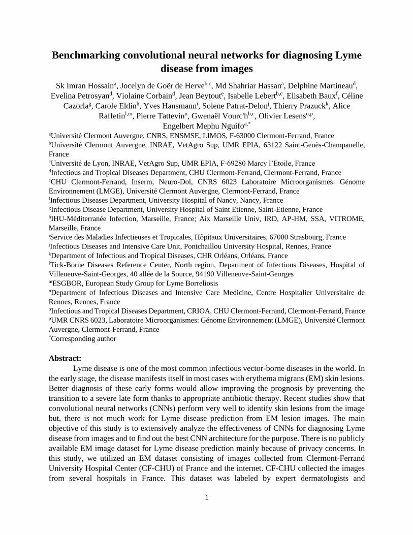
as erythema migrans (EM) becomes visible in the victim’s body which is the most common early

symptom of Lyme disease (Burlina et al., 2018; Shapiro, 2014). EM usually appears at the site of

a tick bite after one to two weeks (range, 3 to 30 days) as a small redness and expands almost a

centimeter per day, creating the characteristic bull’s-eye pattern as shown in Figure 1 (a) (Berglund

et al., 1995; Burlina et al., 2018; Shapiro, 2014; Strle and Stanek, 2009). EM generally vanishes

within a few weeks or months but the Lyme disease infection advances to affect the nervous

system, skin, joints, eyes, and heart (Ružić-Sabljić et al., 2000; Shapiro, 2014; Steere et al., 2004;

Strle and Stanek, 2009). Antibiotics can be used as a medium of effective treatment in the early

stage of Lyme disease. So, early recognition of EM is extremely important to avoid long-term

complications of Lyme disease. The diagnosis of EM is a challenging task because EM can create

different patterns instead of the trademark bull’s-eye pattern as shown in Figure 1 (b).

Diagnosing skin disorders requires a careful inspection from dermatologists or

infectiologists but their availability, especially in rural areas is scarce (Feng et al., 2018; Resneck

and Kimball, 2004). As a result, the diagnosis is generally carried out by non-specialists, and their

diagnostic accuracy is in the range of twenty-four to seventy percent (Federman, 1999; Federman

and Kirsner, 1997; Johnson, 1994; Moreno et al., 2007; Ramsay and Weary, 1996; Seth et al.,

2017; Tran et al., 2005). The wrong diagnosis can result in improper or delayed treatment which

can be harmful to the patient.

3

Artificial intelligence (AI) powered diagnostic tools can help with the scarcity of expert

dermatologists. Recent advancement of deep learning techniques has eased the creation of AI

solutions to aid in skin disorder diagnosis. Many works have been done utilizing deep learning

techniques specifically convolutional neural networks (CNNs) for diagnosing cancerous and other

common skin lesions from dermoscopic images (Brinker et al., 2019; Codella et al., 2018; Cruz-

Roa et al., 2013; Haenssle et al., 2018; Maron et al., 2019; Pérez et al., 2021; Tschandl et al., 2019;

Yuan et al., 2017). As dermoscopic images require dermatoscopes from dermatology clinics other

works have focused on diagnosing skin diseases using deep learning from clinical images (Esteva

et al., 2017; Han et al., 2018; Liu et al., 2020; Sun et al., 2016; J. Yang et al., 2018). According to

some of these studies, deep learning-based systems compete on par with expert dermatologists for

diagnosing diseases from dermoscopic and clinical images (Brinker et al., 2019; Esteva et al.,

2017; Haenssle et al., 2018; Han et al., 2018; Maron et al., 2019).

Despite the vast application of AI in the field of skin lesion diagnosis, there are only a few

works related to Lyme disease detection from EM skin lesion images. The unavailability of public

EM datasets as a result of privacy concerns of medical data may be the reason for the lack of

extensive studies in this field. Čuk et al. (2014) proposed a visual system for EM recognition on a

private EM dataset using classical machine learning techniques including naïve Bayes, SVM,

boosting, and neural nets (not deep learning). Burlina et al. (2018) created a dataset of EM by

collecting images from the internet and trained a CNN architecture ResNet50 as a binary classifier

to distinguish between EM and other skin conditions. Although their dataset is not public, the

trained model is publicly available. Burlina et al., (2020) further enriched the dataset with more

images from the East Coast and Upper Midwest of the United States and trained six CNNs namely

ResNet50, InceptionV3, MobileNetV2, DeneNet121, InceptionResNetV2, and ResNet152 for EM

classification. Burlina et al. (2020) did not make the dataset or the trained models public. Burlina

et al. (2018) and Burlina et al. (2020) used transfer learning from ImageNet (Russakovsky et al.,

2015) pre-trained models and studied the CNNs in terms of predictive performance. With the

advancement of CNNs, it is a timely need to extensively study their effectiveness for Lyme disease

prediction from EM images.

(a) Bull’s-eye pattern (b) Atypical pattern

Figure 1: Patterns of erythema migrans (EM).

(source: https://commons.wikimedia.org/wiki/Category:Erythema_migrans,

Accessed April 1, 2021)

4

In this article, our main objective was to study the performance of state-of-the-art CNNs

for diagnosing Lyme disease from EM images and to find out the best architecture based on

different criteria. As there is no publicly available Lyme dataset of EM images, first, we created a

dataset consisting of 866 images of confirmed EM lesions. Images collected from the internet and

Clermont-Ferrand University Hospital Center (CF-CHU) of France were carefully labeled into two

classes: EM and Confuser, by expert dermatologists and infectiologists from CF-CHU. CF-CHU

collected the images from several hospitals in France. We benchmarked twenty-three well-known

DCCNs on this dataset in terms of several predictive performance metrics, computational

complexity metrics, and statistical significance tests. Best practices for training CNNs on limited

data like transfer learning and data augmentation were used. Second, instead of only using transfer

learning from models pre-trained on ImageNet dataset we also utilized a dataset of common skin

lesions “Human Against Machine with 10000 training images (HAM1000)” (Tschandl et al., 2018)

for pretraining the CNNs. The use of HAM1000 proved fruitful according to the experimental

results. We experimentally searched for the best performing number of layers to unfreeze during

transfer learning fine-tuning for each of the studied CNNs. Third, for visualizing the regions of the

input image that are significant for predictions from the CNN models we used Gradient-weighted

Class Activation Mapping (Grad-CAM) (Selvaraju et al., 2020). Fourth, we provided guidelines

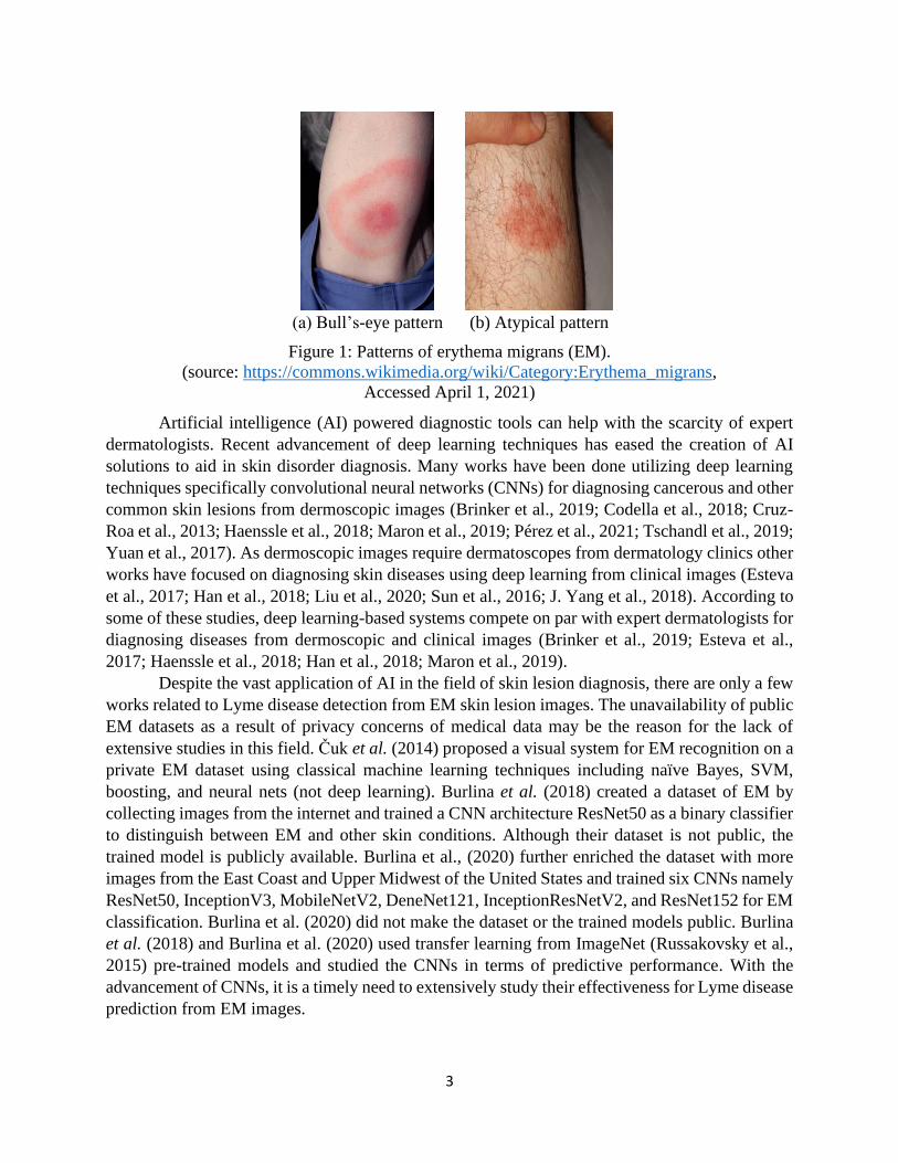
Figure 2: Graphical overview of the study on the effectiveness of CNNs for the diagnosis of

Lyme disease from images.

Erythema Migrans

Novel Lyme Dataset

Which is the best CNN architecture

to diagnosis Lyme disease from images?

Confuser

Exp

erim

enta

l A

nal

ysi

s

Predictive Performance

Model Complexity

Statistical Significance

Explainability via

Grad-CAM visualization

Outc

om

e Recommendation for

CNN architecture selection

Trained CNN models made public which can

be used by others for creating Lyme disease

pre-scanner and doing transfer learning

Confuser

23 CNN Architectures

Custom Transfer Learning

HAM10000

Erythema Migrans

5

for model selection based on predictive performance and computational complexity. Moreover,

we made all the trained models publicly available which can be used for transfer learning and

building pre-scanners for Lyme disease. Figure 2 presents the graphical overview of this study.

The rest of the paper is structured as follows: Section 2 contains dataset description, a brief

overview of CNN architectures, performance measures, and transfer learning approach used in this

study; Section 3 presents experimental studies; Section 4 contains recommendations for model

selection, discussion on limitations and scopes; finally, Section 5 presents concluding remarks.

2. Methods:

The following subsections describe the data organization including data augmentation and

cross-validation, a short overview of the considered CNN architectures, performance measures,

explainability method, and the transfer learning approach used in this study.

2.1. Dataset Preparation:

As a labeled public dataset is not available for Lyme disease prediction from EM images,

we created a dataset by collecting images from the internet and CF-CHU. CF-CHU collected EM

images from several hospitals located in France. The use of images from the internet was inspired

by related skin lesion analysis studies (Burlina et al., 2018, 2020; Esteva et al., 2017). Duplicate

images were removed using an image hashing-based duplicate image detector followed by the

removal of inappropriate images through human inspection. After the initial curation steps, we got

a total of 1672 images. Expert dermatologists and infectiologists from CF-CHU classified the

curated images into two categories: EM and Confuser, making it a two-class classification

problem. Out of 1672 images, 866 images were assigned to EM class and 806 images were

assigned to Confuser class.

We further subdivided the dataset into five-folds using stratified five-fold cross-validation

to make sure each of the folds maintains the original class ratio. One of the folds was used as a test

set and the remaining four were used as the training set with a rotation of the folds for five runs.

Each time, 10% of the training data was assigned to the validation set as shown in Figure 3.

DCCNs require a considerable amount of data for training and data augmentation can help

with expanding the dataset. We applied data augmentation techniques only to the training set to

expand it twenty times. We used flip, rotation, brightness, contrast, and saturation augmentation

Figure 3: Five-fold cross-validation setup.

TRAIN TRAIN TRAIN TRAIN TEST

10%

VALIDATION

Stratified split of 866 erythema migrans (EM) and 806 Confuser images

6

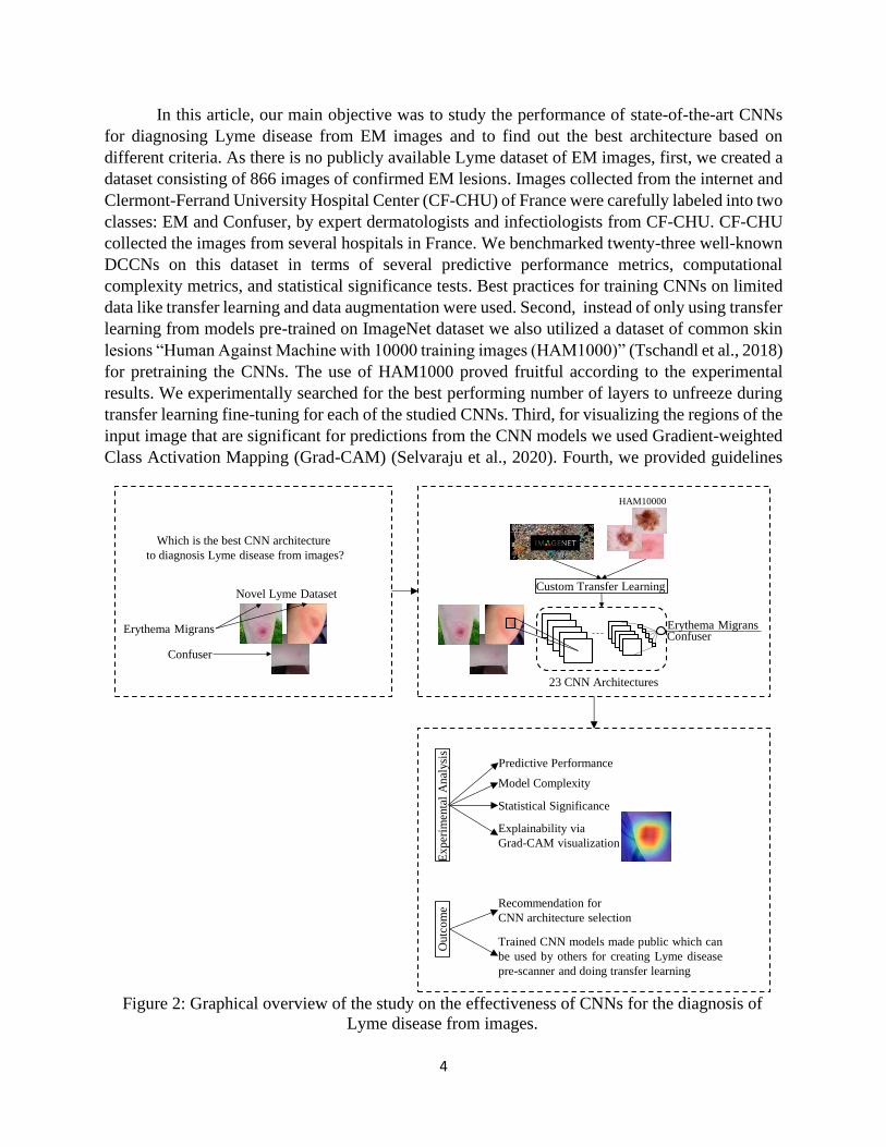
by considering the best performing augmentations for skin lesions (Perez et al., 2018). Besides,

we also used perspective skew transformation to cover the case of looking at a picture from

different angles. Figure 4 shows some example images resulting from augmentations applied on a

sample image. Augmentor (Bloice et al., 2019) an image augmentation library specially built for

biomedical image augmentation was used for applying the augmentations.

2.2. Brief Overview of CNN Architectures for Lyme Disease Diagnosis:

CNNs are a kind of neural network that simulates some actions generated in the human

visual cortex using convolution mathematical operation to extract features from input, and passing

these features through successive layers generates more abstract features to yield a final output

(LeCun et al., 1998). CNNs are modular in design, where convolution-based building blocks are

repeatedly stacked for feature extraction with pooling layers placed in between for reducing feature

space, learnable parameters, and controlling overfitting (Goodfellow et al., 2016). Starting with

LeNet (LeCun et al., 1998) in 1988 the popularity of CNNs increased with AlexNet (Krizhevsky

et al., 2017) winning the ImageNet Large Scale Visual Recognition Challenge (ILSVRC)

(Russakovsky et al., 2015) of 2012. As a result of the effectiveness of CNNs in solving complex

problems, several CNN architectures have been introduced over the past few years. The following

subsections provide a brief overview of the CNN architectures used in this study for diagnosing

Lyme disease from EM images.

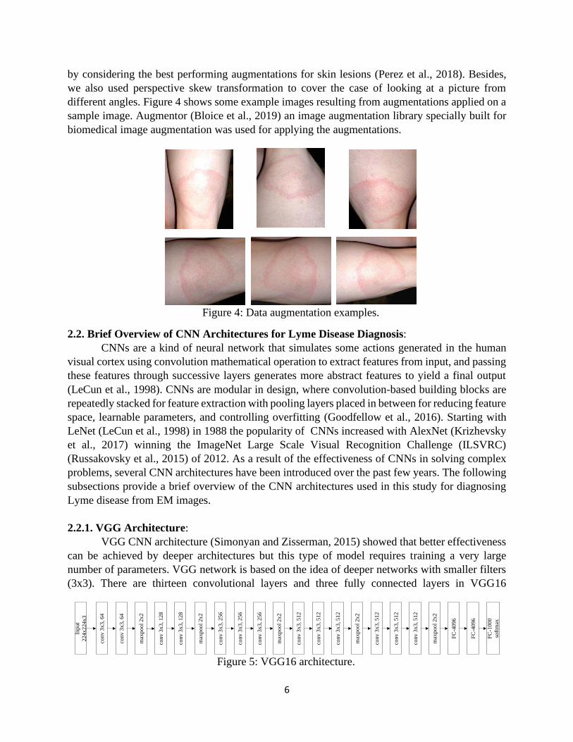
2.2.1. VGG Architecture:

VGG CNN architecture (Simonyan and Zisserman, 2015) showed that better effectiveness

can be achieved by deeper architectures but this type of model requires training a very large

number of parameters. VGG network is based on the idea of deeper networks with smaller filters

(3x3). There are thirteen convolutional layers and three fully connected layers in VGG16

Figure 5: VGG16 architecture.

Input

224x

224x

3

conv 3

x3, 64

max

pool

2x

2

conv 3

x3, 64

conv 3

x3, 128

conv 3

x3, 256

max

pool

2x

2

conv 3

x3, 128

conv 3

x3, 256

conv 3

x3, 256

max

pool

2x

2

conv 3

x3, 512

conv 3

x3, 512

conv 3

x3, 512

max

pool

2x

2

conv 3

x3, 512

conv 3

x3, 512

conv 3

x3, 512

max

pool

2x

2

FC

-40

96

FC

-40

96

FC

-10

00

soft

max

Figure 4: Data augmentation examples.

7

architecture as shown in Figure 5. Another variation of VGG architecture called VGG19 has

sixteen convolutional layers and three fully connected layers. To the best of our knowledge, VGG

architectures have not been used previously for Lyme disease analysis.

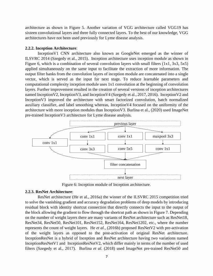
2.2.2. Inception Architecture:

InceptionV1 CNN architecture also known as GoogleNet emerged as the winner of

ILSVRC 2014 (Szegedy et al., 2015). Inception architecture uses inception module as shown in

Figure 6, which is a combination of several convolution layers with small filters (1x1, 3x3, 5x5)

applied simultaneously on the same input to facilitate the extraction of more information. The

output filter banks from the convolution layers of inception module are concatenated into a single

vector, which is served as the input for next stage. To reduce learnable parameters and

computational complexity inception module uses 1x1 convolution at the beginning of convolution

layers. Further improvement resulted in the creation of several versions of inception architectures

named InceptionV2, InceptionV3, and InceptionV4 (Szegedy et al., 2017, 2016). InceptionV2 and

InceptionV3 improved the architecture with smart factorized convolution, batch normalized

auxiliary classifier, and label smoothing whereas, InceptionV4 focused on the uniformity of the

architecture with more inception modules than InceptionV3. Burlina et al., (2020) used ImageNet

pre-trained InceptionV3 architecture for Lyme disease analysis.

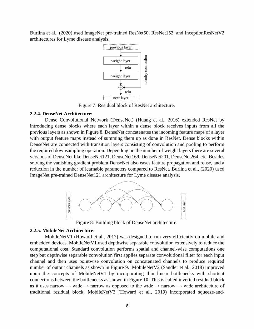
2.2.3. ResNet Architecture:

ResNet architecture (He et al., 2016a) the winner of the ILSVRC 2015 competition tried

to solve the vanishing gradient and accuracy degradation problems of deep models by introducing

residual block with identity shortcut connection that directly connects the input to the output of

the block allowing the gradient to flow through the shortcut path as shown in Figure 7. Depending

on the number of weight layers there are many variants of ResNet architecture such as ResNet18,

ResNet34, ResNet50, ResNet101, ResNet152, ResNet164, ResNet1202, etc., where the number

represents the count of weight layers. He et al., (2016b) proposed ResNetV2 with pre-activation

of the weight layers as opposed to the post-activation of original ResNet architecture.

InceptionResNet is a hybrid of Inception and ResNet architecture having two variations named

InceptionResNetV1 and InceptionResNetV2, which differ mainly in terms of the number of used

filters (Szegedy et al., 2017). Burlina et al. (2018) used ImageNet pre-trained ResNet50 and

Figure 6: Inception module of Inception architecture.

previous layer

conv 1x1 conv 1x1 maxpool 3x3

conv 3x3 conv 5x5 conv 1x1

conv 1x1

filter concatenation

next layer

8

Burlina et al., (2020) used ImageNet pre-trained ResNet50, ResNet152, and InceptionResNetV2

architectures for Lyme disease analysis.

2.2.4. DenseNet Architecture:

Dense Convolutional Network (DenseNet) (Huang et al., 2016) extended ResNet by

introducing dense blocks where each layer within a dense block receives inputs from all the

previous layers as shown in Figure 8. DenseNet concatenates the incoming feature maps of a layer

with output feature maps instead of summing them up as done in ResNet. Dense blocks within

DenseNet are connected with transition layers consisting of convolution and pooling to perform

the required downsampling operation. Depending on the number of weight layers there are several

versions of DenseNet like DenseNet121, DenseNet169, DenseNet201, DenseNet264, etc. Besides

solving the vanishing gradient problem DenseNet also eases feature propagation and reuse, and a

reduction in the number of learnable parameters compared to ResNet. Burlina et al., (2020) used

ImageNet pre-trained DenseNet121 architecture for Lyme disease analysis.

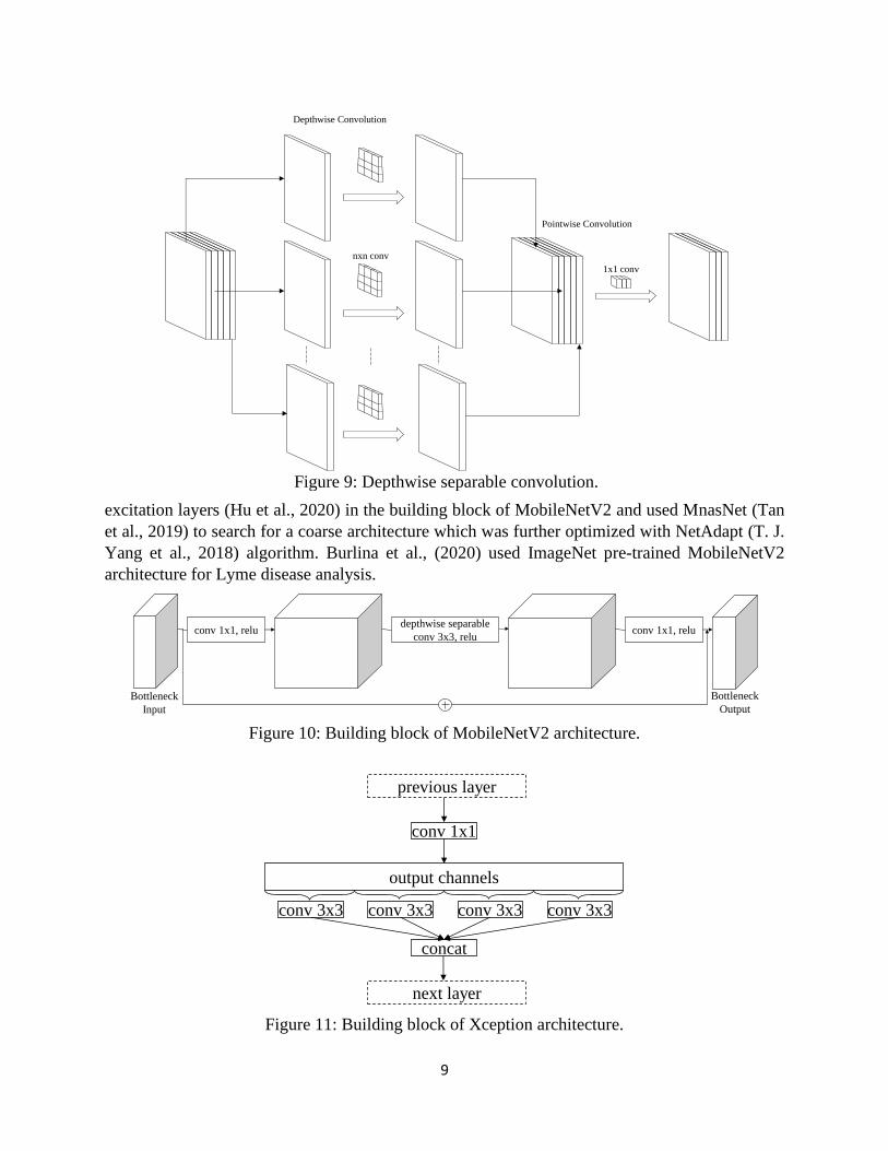
2.2.5. MobileNet Architecture:

MobileNetV1 (Howard et al., 2017) was designed to run very efficiently on mobile and

embedded devices. MobileNetV1 used depthwise separable convolution extensively to reduce the

computational cost. Standard convolution performs spatial and channel-wise computations one

step but depthwise separable convolution first applies separate convolutional filter for each input

channel and then uses pointwise convolution on concatenated channels to produce required

number of output channels as shown in Figure 9. MobileNetV2 (Sandler et al., 2018) improved

upon the concepts of MobileNetV1 by incorporating thin linear bottlenecks with shortcut

connections between the bottlenecks as shown in Figure 10. This is called inverted residual block

as it uses narrow → wide → narrow as opposed to the wide → narrow → wide architecture of

traditional residual block. MobileNetV3 (Howard et al., 2019) incorporated squeeze-and-

Figure 7: Residual block of ResNet architecture.

weight layer

weight layer

iden

tity

connec

tion

relu

relu

previous layer

next layer

Figure 8: Building block of DenseNet architecture.

pre

vio

us

layer

nex

t la

yer

9

excitation layers (Hu et al., 2020) in the building block of MobileNetV2 and used MnasNet (Tan

et al., 2019) to search for a coarse architecture which was further optimized with NetAdapt (T. J.

Yang et al., 2018) algorithm. Burlina et al., (2020) used ImageNet pre-trained MobileNetV2

architecture for Lyme disease analysis.

Figure 9: Depthwise separable convolution.

nxn conv

1x1 conv

Depthwise Convolution

Pointwise Convolution

Figure 10: Building block of MobileNetV2 architecture.

depthwise separable

conv 3x3, relu conv 1x1, relu conv 1x1, relu

Bottleneck

Input

Bottleneck

Output

Figure 11: Building block of Xception architecture.

conv 1x1

output channels

conv 3x3 conv 3x3 conv 3x3 conv 3x3

concat

previous layer

next layer

10

2.2.6. Xception architecture:

Extreme version of Inception the Xception architecture (Chollet, 2017) replaced the

Inception module with a modified version of depthwise separable convolution where the order of

depthwise convolution and pointwise convolutions are reversed as shown in Figure 11. Xception

also uses shortcut connections like ResNet architecture. On ImageNet dataset Xception performs

slightly better than the InceptionV3 architecture. To the best of our knowledge, Xception

architecture has not been used previously for Lyme disease analysis.

2.2.7. NASNet architecture:

Neural Architecture Search Netowork (Zoph et al., 2018) from Google Brain utilizes

reinforcement learning with a Recurrent Neural Network based controller to search for efficient

building block for a smaller dataset which is then transferred to a larger dataset by stacking

multiple copies of the found building block. NASNet blocks are comprised of normal and

reduction cells as shown in Figure 12. Normal cells produce feature map of same size as input

whereas reduction cells reduce the size by a factor of two. NASNet optimized for mobile

applications is called NASNetMobile whereas the larger version is called NASNetLarge. To the

best of our knowledge, NASNet architectures have not been used previously for Lyme disease

analysis.

2.2.8. EfficientNet architecture:

EfficientNet (Tan and Le, 2019) which is among the most efficient models proposed a

scaling method to uniformly scale all dimensions of depth, width, and resolution of a network

using a compound coefficient. The baseline network of EfficientNet was built with neural

architecture search incorporating squeeze-and-excitation in the building block of MobileNetV2.

The scaling method is defined as:

𝑑𝑒𝑝𝑡ℎ = 𝛼∅

width = 𝛽∅

resolution = 𝛾∅ ,

s.t. 𝛼. 𝛽2. 𝛾2 ≈ 2; 𝛼 ≥ 1, 𝛽 ≥ 1, 𝛾 ≥ 1

(1)

where, the coefficient ∅ controls available resources and 𝛼, 𝛽, and 𝛾 are constants obtained

by grid search. EfficientNetB0-B7 are a family of architectures scaled up from the baseline

network that reflects a good balance of accuracy and efficiency. To the best of our knowledge,

EfficientNet architectures have not been used previously for Lyme disease analysis.

Figure 12: Building block of NASNet architecture.

normal cell

reduction cell

previous layer

next layer

11

2.3. Predictive Performance Measures:

To compare the predictive performance of the trained CNN models we used accuracy,

recall/sensitivity/hit rate/true positive rate (TPR), specificity/selectivity/true negative rate (TNR),

precision/ positive predictive value (PPV), negative predictive value (NPV), Matthews correlation

coefficient (MCC), Cohen’s kappa coefficient (𝜅), positive likelihood ratio (LR+), negative

likelihood ratio (LR-), F1-score, confusion matrix and area under the receiver operating

characteristic (ROC) curve (AUC) metrics. Confusion matrix is a way of presenting the count of

true negatives (TN), false positives (FP), false negatives (FN), and true positives (TP) in a matrix

format where the y-axis presents true labels and x-axis presents predicted labels. Accuracy

measures the proportion of correctly classified predictions among all the predictions, and it is

calculated as:

𝐴𝑐𝑐𝑢𝑟𝑎𝑐𝑦 =

𝑇𝑃 + 𝑇𝑁

𝑇𝑃 + 𝑇𝑁 + 𝐹𝑃 + 𝐹𝑁

(2)

Recall/sensitivity/hit rate/TPR measures the proportion of actual positives correctly identified, and

it is expressed as:

𝑅𝑒𝑐𝑎𝑙𝑙, 𝑆𝑒𝑛𝑠𝑖𝑡𝑖𝑣𝑖𝑡𝑦, ℎ𝑖𝑡 𝑟𝑎𝑡𝑒, 𝑇𝑃𝑅 =

𝑇𝑃

𝑇𝑃 + 𝐹𝑁

(3)

Specificity/selectivity/ TNR measures the proportion of actual negatives correctly identified, and

it is expressed as:

𝑆𝑝𝑒𝑐𝑖𝑓𝑖𝑐𝑖𝑡𝑦, 𝑆𝑒𝑙𝑒𝑐𝑡𝑖𝑣𝑖𝑡𝑦, 𝑇𝑁𝑅 =

𝑇𝑁

𝑇𝑁 + 𝐹𝑃

(4)

Precision/ PPV measures the proportion of correct positive predictions, and it is calculated as:

𝑃𝑟𝑒𝑐𝑖𝑠𝑖𝑜𝑛, 𝑃𝑃𝑉 =

𝑇𝑃

𝑇𝑃 + 𝐹𝑃

(5)

NPV measures the proportion of negative predictions that are correct, and it is calculated as:

𝑁𝑃𝑉 =

𝑇𝑁

𝑇𝑁 + 𝐹𝑁

(6)

MCC provides a summary of the confusion matrix, and it is calculated as:

𝑀𝐶𝐶 =

𝑇𝑃 ∗ 𝑇𝑁 − 𝐹𝑃 ∗ 𝐹𝑁

√(𝑇𝑃 + 𝐹𝑃)(𝑇𝑃 + 𝐹𝑁)(𝑇𝑁 + 𝐹𝑃)(𝑇𝑁 + 𝐹𝑁)

(7)

MCC value is in the range [−1, +1], where 0 is like random prediction, +1 means a perfect

prediction, and −1 represents inverse prediction. Cohen’s kappa coefficient (𝜅) metric is used to

assess inter-rater agreement which tells us how the model is performing compared to a random

classifier, and it is calculated with the formula:

𝜅 =𝑝𝑜 − 𝑝𝑒

1 − 𝑝𝑒 (8)

where, 𝑝𝑜 is the relative observed agreement among the raters and 𝑝𝑒 is the hypothetical probability

of expected agreement which is defined for 𝑐 categories as:

𝑝𝑒 =

1

𝑁2∑ 𝑛𝑐1𝑛𝑐2

𝑐

(9)

where, 𝑁 is the total number of observations, and 𝑛𝑐𝑟 is the number of predictions of category 𝑐

by rater 𝑟. Value of 𝜅 is in the range [−1, +1], where a value of 1 indicates perfect agreement, 0

means agreement only by chance, and a negative value indicates the agreement is worse than the

12

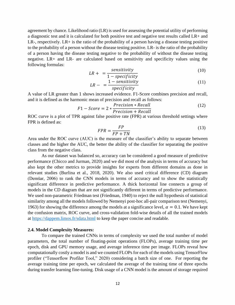
agreement by chance. Likelihood ratio (LR) is used for assessing the potential utility of performing

a diagnostic test and it is calculated for both positive test and negative test results called LR+ and

LR-, respectively. LR+ is the ratio of the probability of a person having a disease testing positive

to the probability of a person without the disease testing positive. LR- is the ratio of the probability

of a person having the disease testing negative to the probability of without the disease testing

negative. LR+ and LR- are calculated based on sensitivity and specificity values using the

following formulas:

𝐿𝑅 + =

𝑠𝑒𝑛𝑠𝑖𝑡𝑖𝑣𝑖𝑡𝑦

1 − 𝑠𝑝𝑒𝑐𝑖𝑓𝑖𝑐𝑖𝑡𝑦

(10)

𝐿𝑅 − =

1 − 𝑠𝑒𝑛𝑠𝑖𝑡𝑖𝑣𝑖𝑡𝑦

𝑠𝑝𝑒𝑐𝑖𝑓𝑖𝑐𝑖𝑡𝑦

(11)

A value of LR greater than 1 shows increased evidence. F1-Score combines precision and recall,

and it is defined as the harmonic mean of precision and recall as follows:

𝐹1 − 𝑆𝑐𝑜𝑟𝑒 = 2 ∗

𝑃𝑟𝑒𝑐𝑖𝑠𝑖𝑜𝑛 ∗ 𝑅𝑒𝑐𝑎𝑙𝑙

𝑃𝑟𝑒𝑐𝑖𝑠𝑖𝑜𝑛 + 𝑅𝑒𝑐𝑎𝑙𝑙

(12)

ROC curve is a plot of TPR against false positive rate (FPR) at various threshold settings where

FPR is defined as:

𝐹𝑃𝑅 =

𝐹𝑃

𝐹𝑃 + 𝑇𝑁

(13)

Area under the ROC curve (AUC) is the measure of the classifier’s ability to separate between

classes and the higher the AUC, the better the ability of the classifier for separating the positive

class from the negative class.

As our dataset was balanced so, accuracy can be considered a good measure of predictive

performance (Chicco and Jurman, 2020) and we did most of the analysis in terms of accuracy but

also kept the other metrics to provide insights for experts from different domains as done in

relevant studies (Burlina et al., 2018, 2020). We also used critical difference (CD) diagram

(Demšar, 2006) to rank the CNN models in terms of accuracy and to show the statistically

significant difference in predictive performance. A thick horizontal line connects a group of

models in the CD diagram that are not significantly different in terms of predictive performance.

We used non-parametric Friedman test (Friedman, 1940) to reject the null hypothesis of statistical

similarity among all the models followed by Nemenyi post-hoc all-pair comparison test (Nemenyi,

1963) for showing the difference among the models at a significance level, 𝛼 = 0.1. We have kept

the confusion matrix, ROC curve, and cross-validation fold-wise details of all the trained models

at https://dappem.limos.fr/sdata.html to keep the paper concise and readable.

2.4. Model Complexity Measures:

To compare the trained CNNs in terms of complexity we used the total number of model

parameters, the total number of floating-point operations (FLOPs), average training time per

epoch, disk and GPU memory usage, and average inference time per image. FLOPs reveal how

computationally costly a model is and we counted FLOPs for each of the models using TensorFlow

profiler (“Tensorflow Profiler Tool,” 2020) considering a batch size of one. For reporting the

average training time per epoch, we calculated the average of the training time of three epochs

during transfer learning fine-tuning. Disk usage of a CNN model is the amount of storage required

13

to save the model architecture along with weights. We calculated the GPU usage of a CNN model

by inspecting the memory allocated in GPU after loading a trained instance of the model. To

measure the average inference time per image of a model we took the average of three hundred

inferences on the same input image.

2.5. Model Explainability:

Explainability is important for AI tools especially in the case of medical applications

(Vellido, 2020). We used Grad-CAM explainability technique for visualizing the regions of the

input image that are significant for predictions from the CNN models as shown in Figure 13. Grad-

CAM uses gradient flowing into the ultimate convolution layer for producing heatmaps, and it is

a kind of post-hoc attention that can be applied on an already trained model. Grad-CAM provides

similar result to occlusion sensitivity map (Zeiler and Fergus, 2014) that works by masking

patches of the input image but Grad-CAM is much faster to calculate compared to image occlusion

(Selvaraju et al., 2020).

2.6. Transfer Learning Approach:

In this study, we used transfer learning as our Lyme dataset is not huge enough to obtain

good performance by training large CNNs from scratch. We started with a CNN already pre-

Figure 13: Gard-CAM visualization example.

Input Image Grad-CAM Visualization

Figure 14: Transfer learning workflow used in this study. GAP stands for Global Average

Polling. N is the number of ImageNet pre-trained layers and U represents the number of layers

used for fine-tuning.

Fro

zen

Fro

zen

Fro

zen

1 2 3 N-U+1 N-U+2 N

ImageNet pretrained DCNN

GA

P

dro

pout

FC

-1

sigm

oid

EM classifier head

HAM10000

pretraining

Lyme dataset

training

14

trained on ImageNet dataset and after removing the original ImageNet classification head our EM

classification head consisting of Global Average Pooling (GAP) layer, dropout layer, and a fully

connected layer with sigmoid activation for binary classification was added as shown in Figure 14.

According to our experiments fine-tuning the whole CNN architecture after training the classifier

head with our Lyme dataset performed poorly compared to the partial fine-tuning of several layers

at the end of the CNN while keeping rest of the layers frozen. We empirically found out the number

of layers 𝑈 to fine-tune from 𝑁 number of ImageNet pre-trained layers for each of the CNN

architectures used in this study. According to the experimental results pretraining the unfrozen part

with HAM10000 dataset further improved the performance of the DCCNs.

3. Experimental Studies:

The following subsections describe experimental settings including model selection and

parameter settings, software and hardware used for the study, the experimental results, and

recommendations for model selection.

3.1. Experimental Settings:

In this study, we benchmarked twenty-three CNN models, namely VGG16, VGG19,

ResNet50, ResNet101, ResNet50V2, ResNet101V2, InceptionV3, InceptionV4,

InceptionResNetV2, Xception, DenseNet121, DenseNet169, DenseNet201, MobileNetV2,

MobileNetV3Large, MobileNetV3Small, NASNetMobile, EfficientNetB0, EfficientNetB1,

EfficientNetB2, EfficientNetB3, EfficientNetB4, and EfficientNetB5 for diagnosing Lyme disease

from EM images. These models were selected to explore a diverse set of CNN models covering

various prospects, like different architectures, depths, and complexities.

To the best of our knowledge ResNet50 is the only publicly available trained CNN that

was used for Lyme disease identification by Burlina et al., (2018). We are calling this model

ResNet50-Burlina which is a collection of five models (trained on five-fold cross-validation data)

available at https://github.com/neil454/lyme-1600-model. We did extensive analysis on the

ResNet50 architecture using seven different transfer learning configurations: (i) training ResNet50

model on our Lyme dataset from scratch without using transfer learning (called ResNet50-NTL,

where, NTL stands for no transfer learning), (ii) pretraining ResNet50 model with only

HAM10000 data followed by fine-tuning all the layers with our Lyme dataset (called ResNet50-

HAM-FFT, where HAM means HAM10000 and FFT stands for full fine-tuning), (iii) training

only the EM classifier head of an ImageNet pre-trained ResNet50 model with our Lyme dataset

(called ResNet50-IMG-WFT, where IMG means ImageNet and WFT stands for without fine-

tuning), (iv) fine-tuning all the layers of ImageNet pre-trained ResNet50 model with our Lyme

dataset (called ResNet50-IMG-FFT), (v) fine-tuning 𝑈 no of layers of an ImageNet pre-trained

ResNet50 model with our Lyme dataset (called ResNet50-IMG-FT𝑈, where FT𝑼 means fine-

tuning 𝑈 no of layers), (vi) pretraining the whole ImgaeNet pre-trained ResNet50 model by

HAM10000 data before fine-tuning 𝑈 layers with our Lyme dataset (called ResNet50-IMG-

HAMFP-FT𝑈, where, HAMFP means full pre-training with HAM10000 dataset), and (vii)

pretraining only the unfrozen 𝑈 layers of a ImgaeNet pre-trained ResNet50 model with

HAM10000 data before fine-tuning 𝑈 layers with our Lyme dataset (called ResNet50-IMG-

HAMPP-FT𝑈, where, HAMPP means partial pre-training with HAM10000 dataset). According

15

to experimental results (discussed below), ResNet50-IMG-HAMPP-FT𝑈 configuration performed

best, and we used this configuration (pretraining only the unfrozen 𝑈 layers of an ImgaeNet pre-

trained model with HAM10000 data before fine-tuning 𝑈 layers with our Lyme dataset) for

training all the architectures used in this study. For simplicity, the best performing trained models

of each of the architectures are presented in ModelName-𝑼 format, where 𝑈 represents the no of

unfrozen layers. For example, EfficientNetB0-187 means EfficientNetB0-IMG-HAMPP-FT187

and ResNet50-141 means ResNet50-IMG-HAMPP-FT141.

For training all the models, we used a dropout rate of 0.2 for the dropout layer in EM

classifier head section. Adaptive Moment Estimation (ADAM) (Kingma and Ba, 2015) optimizer

with exponential decay rate for the first and second moment estimates set to 0.9 and 0.999

respectively was used with a learning rate of 0.0001 for training the classifier head and 0.00001

for fine-tuning. We also used early stopping to terminate the training if there was no improvement

in validation accuracy for ten epochs. A batch size of 32 was used. For reporting the number of

layers to unfreeze during transfer learning, we stated the total number of layers to unfreeze

including layers containing both trainable and non-trainable parameters.

We used three NVIDIA QUADRO RTX 8000 GPUs and two Desktop Computers with

Intel Xeon W-2175 processor, 64 GB DDR4 RAM, and Ubuntu 18.04 operating system to perform

all the experiments. Python v3.6.9, and TensorFlow v2.4.1 platform (Abadi et al., 2016) were used

for all the implementations and experimentations of this study.

3.2. Experimental Results:

Čuk et al., (2014) reported accuracies in the range of 69.23% to 80.42% using classical

machine learning methods whereas, Burlina et al., (2020) reported the best accuracy of 81.51%

using ResNet50 architecture for the case of EM vs all classification problems. There was a

common subset of images collected from the internet in both the dataset of Burlina et al., (2018)

and our Lyme dataset. ResNet50-Burlina model gave an accuracy of 76.05% when tested on our

full dataset as shown in Table 1.

Table 1: Performance metrics of ResNet50-Burlina model trained by Burlina et al., (2018) tested

on the whole dataset of this study. Within each cell, the value after (±) symbol represents the

standard deviation.

ResNet50-

Burlina

76.05

±0.74

70.05

±3.6

82.51

±3.31

81.29

±2.1

72.04

±1.71

0.5294

±0.0132

0.5229

±0.0145

4.1017

±0.5172

0.362

±0.0309

0.7515

±0.0137

0.481

±0.0509

ResNet50-NTL model resulting from training ResNet50 architecture from scratch without

transfer learning gave an accuracy of 76.35%. ResNet50-HAM-FFT model resulting from

pretraining ResNet50 architecture with only HAM10000 data followed by fine-tuning of all the

layers with our Lyme dataset showed a degraded accuracy of 72.27%. ResNet50-IMG-WFT,

Model

()%

Metric

16

generated by training only the EM classifier head of an ImageNet pre-trained ResNet50

architecture improved the accuracy to 78.94%. ResNet50-IMG-FFT, resulting from fine-tuning

all the layers of ImageNet pre-trained ResNet50 architecture, further improved the classification

accuracy to 82.22%. Whereas ResNet50-IMG-FT141, model resulting from fine-tuning 141

layers of pre-trained ResNet50 architecture gave an accuracy of 83.24% which is better compared

to unfreezing the full architecture. ResNet50-IMG-HAMFP-FT141, model resulting from

pretraining the whole ImgaeNet pre-trained ResNet50 model by HAM10000 data before fine-

tuning 141 layers with our Lyme dataset reduced the accuracy to 82.35%. But pretraining only

the unfrozen 141 layers with HAM10000 data gave us the model ResNet50-IMG-HAMPP-FT141

with the best accuracy of 84.42%. Figure 15 shows the CD diagram in terms of accuracy for these

ResNet50 based models. We excluded ResNet50-Burlina model from this diagram because the

model was tested on the whole dataset as opposed to other configurations. The Friedman test null

hypothesis was rejected with a 𝑝 value of 0.0002. From the CD diagram, we can see that

ResNet50-IMG-HAMPP-FT141 achieved the best average ranking among the compared models.

Although there is no statistically significant difference among ResNet50-IMG-FFT, ResNet50-

IMG-FT141, ResNet50-IMG-HAMFP-FT141, and ResNet50-IMG-HAMPP-FT141 in terms of

accuracy the ResNet50-IMG-HAMPP-FT141 model performed better in terms of most of the

metrics (7 out of 11) as highlighted in Table 2. To summarize, pretraining only the unfrozen part

of an ImageNet pre-trained CNN with HAM10000 data provided the best accuracy according to

our experiments. So, for all the other CNN architectures, we only reported the performance

resulting from this configuration.

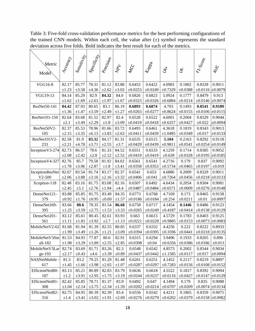
Performance metrics for the best performing configuration of all the CNN architectures

used in this study are shown in Table 3. All these models used HAM1000 pretraining for the

unfrozen part of the network. The number at the end of the model’s name represents the number

of layers unfrozen during transfer learning fine-tuning. ResNet50-141 achieved the best accuracy

of 84.42%. Most of the models except MobileNetV2-62, MobileNetV3Small-182, and

NASNetMobile-617 showed good AUC values of above 90% and good sensitivity suggesting that

these CNNs can be a good choice for building pre-scanners for Lyme disease. Figure 16 shows the

CD diagram in terms of accuracy for these models. The Friedman test null hypothesis was rejected

Figure 15: Accuracy critical difference diagram for ResNet50 models. The models are ordered

by best to worst average ranking from left to right. The number beside a model’s name

represents the average rank of the model. CD is the critical difference for Nemenyi post-hoc

test. Thick horizontal line connects the models that are not statistically significantly different.

17

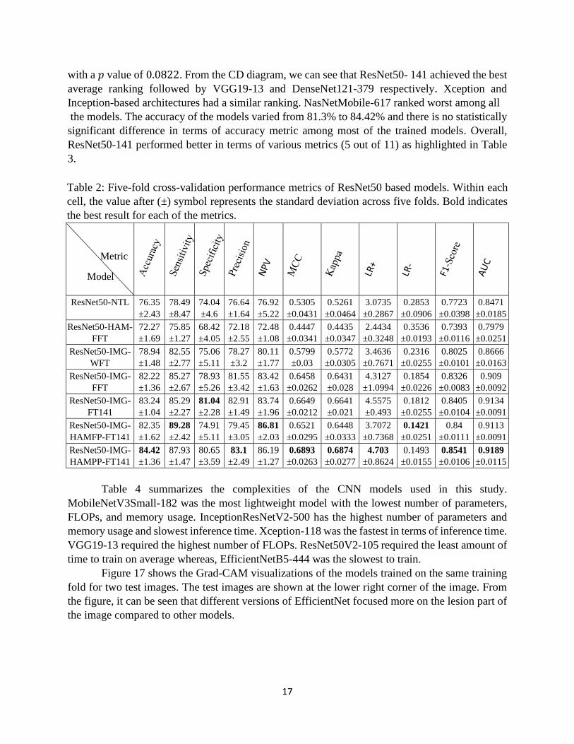
with a 𝑝 value of 0.0822. From the CD diagram, we can see that ResNet50- 141 achieved the best

average ranking followed by VGG19-13 and DenseNet121-379 respectively. Xception and

Inception-based architectures had a similar ranking. NasNetMobile-617 ranked worst among all

the models. The accuracy of the models varied from 81.3% to 84.42% and there is no statistically

significant difference in terms of accuracy metric among most of the trained models. Overall,

ResNet50-141 performed better in terms of various metrics (5 out of 11) as highlighted in Table

3.

Table 2: Five-fold cross-validation performance metrics of ResNet50 based models. Within each

cell, the value after (±) symbol represents the standard deviation across five folds. Bold indicates

the best result for each of the metrics.

ResNet50-NTL

76.35

±2.43

78.49

±8.47

74.04

±4.6

76.64

±1.64

76.92

±5.22

0.5305

±0.0431

0.5261

±0.0464

3.0735

±0.2867

0.2853

±0.0906

0.7723

±0.0398

0.8471

±0.0185

ResNet50-HAM-

FFT

72.27

±1.69

75.85

±1.27

68.42

±4.05

72.18

±2.55

72.48

±1.08

0.4447

±0.0341

0.4435

±0.0347

2.4434

±0.3248

0.3536

±0.0193

0.7393

±0.0116

0.7979

±0.0251

ResNet50-IMG-

WFT

78.94

±1.48

82.55

±2.77

75.06

±5.11

78.27

±3.2

80.11

±1.77

0.5799

±0.03

0.5772

±0.0305

3.4636

±0.7671

0.2316

±0.0255

0.8025

±0.0101

0.8666

±0.0163

ResNet50-IMG-

FFT

82.22

±1.36

85.27

±2.67

78.93

±5.26

81.55

±3.42

83.42

±1.63

0.6458

±0.0262

0.6431

±0.028

4.3127

±1.0994

0.1854

±0.0226

0.8326

±0.0083

0.909

±0.0092

ResNet50-IMG-

FT141

83.24

±1.04

85.29

±2.27

81.04

±2.28

82.91

±1.49

83.74

±1.96

0.6649

±0.0212

0.6641

±0.021

4.5575

±0.493

0.1812

±0.0255

0.8405

±0.0104

0.9134

±0.0091

ResNet50-IMG-

HAMFP-FT141

82.35

±1.62

89.28

±2.42

74.91

±5.11

79.45

±3.05

86.81

±2.03

0.6521

±0.0295

0.6448

±0.0333

3.7072

±0.7368

0.1421

±0.0251

0.84

±0.0111

0.9113

±0.0091

ResNet50-IMG-

HAMPP-FT141

84.42

±1.36

87.93

±1.47

80.65

±3.59

83.1

±2.49

86.19

±1.27

0.6893

±0.0263

0.6874

±0.0277

4.703

±0.8624

0.1493

±0.0155

0.8541

±0.0106

0.9189

±0.0115

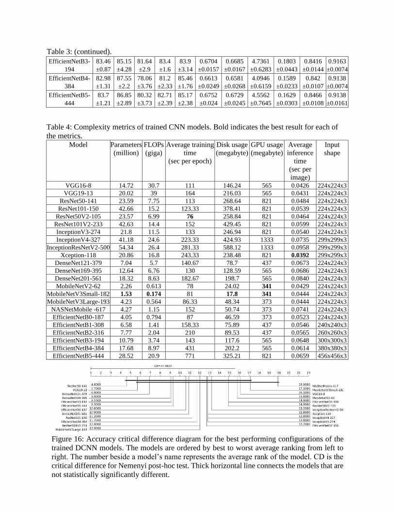
Table 4 summarizes the complexities of the CNN models used in this study.

MobileNetV3Small-182 was the most lightweight model with the lowest number of parameters,

FLOPs, and memory usage. InceptionResNetV2-500 has the highest number of parameters and

memory usage and slowest inference time. Xception-118 was the fastest in terms of inference time.

VGG19-13 required the highest number of FLOPs. ResNet50V2-105 required the least amount of

time to train on average whereas, EfficientNetB5-444 was the slowest to train.

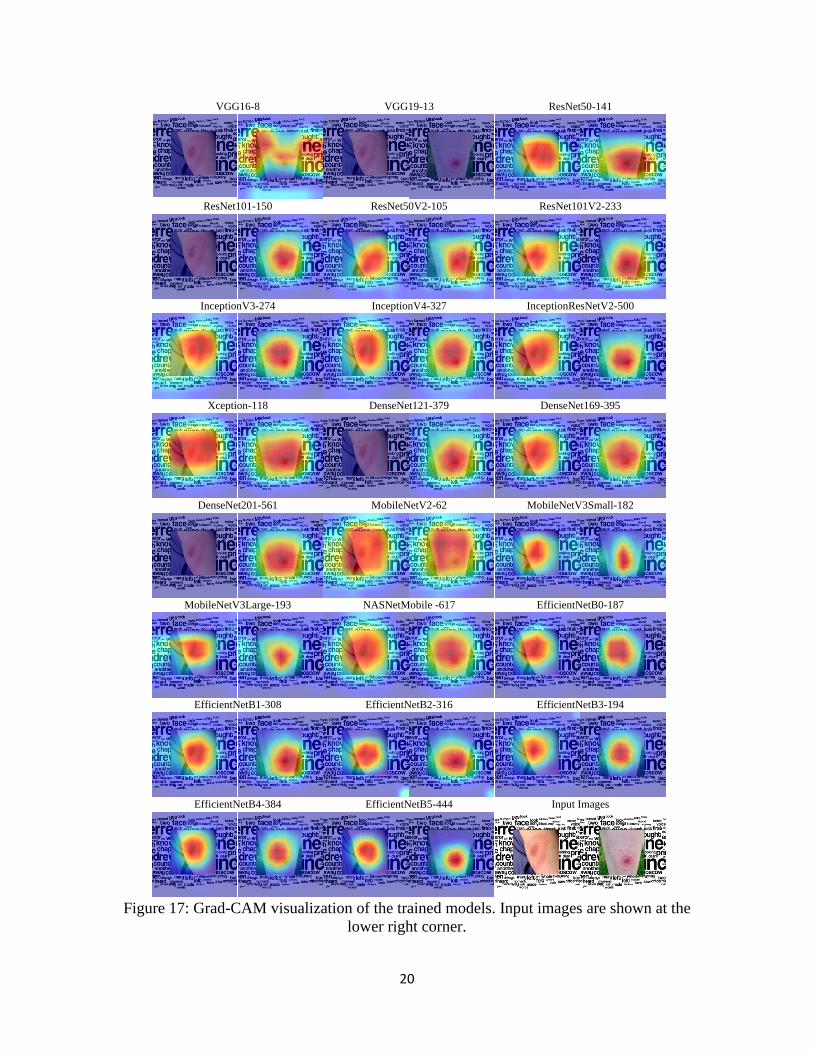
Figure 17 shows the Grad-CAM visualizations of the models trained on the same training

fold for two test images. The test images are shown at the lower right corner of the image. From

the figure, it can be seen that different versions of EfficientNet focused more on the lesion part of

the image compared to other models.

Model

()%

Metric

18

Table 3: Five-fold cross-validation performance metrics for the best performing configurations of

the trained CNN models. Within each cell, the value after (±) symbol represents the standard

deviation across five folds. Bold indicates the best result for each of the metrics.

VGG16-8 82.17

±1.23

85.77

±3.58

78.31

±4.36

81.12

±2.62

83.88

±3.02

0.6453

±0.0253

0.6422

±0.0249

4.0983

±0.7329

0.1802

±0.0388

0.8328

±0.0116

0.9011

±0.0079

VGG19-13 84.14

±1.62

85.29

±1.69

82.9

±2.63

84.32

±1.97

84.0

±1.67

0.6826

±0.0323

0.6823

±0.0326

5.0924

±0.6884

0.1777

±0.0214

0.8479

±0.0146

0.913

±0.0074

ResNet50-141 84.42

±1.36

87.93

±1.47

80.65

±3.59

83.1

±2.49

86.19

±1.27

0.6893

±0.0263

0.6874

±0.0277

4.703

±0.8624

0.1493

±0.0155

0.8541

±0.0106

0.9189

±0.0115

ResNet101-150 82.64

±2.1

83.68

±3.49

81.52

±2.29

82.97

±1.8

82.4

±3.09

0.6528

±0.0419

0.6522

±0.0418

4.6001

±0.6257

0.2004

±0.0427

0.8329

±0.022

0.9044

±0.0094

ResNet50V2-

105

82.37

±2.15

85.53

±3.35

78.96

±6.13

81.66

±3.83

83.72

±2.63

0.6493

±0.0411

0.6461

±0.0439

4.3618

±1.0495

0.1819

±0.0349

0.8343

±0.017

0.9013

±0.0133

ResNet101V2-

233

82.58

±2.21

81.9

±4.78

83.32

±3.71

84.17

±2.55

81.31

±3.7

0.6535

±0.0429

0.6515

±0.0439

5.104

±0.9811

0.2163

±0.0541

0.8292

±0.0254

0.9118

±0.0149

InceptionV3-274 82.73

±2.08

86.57

±2.42

78.6

±2.8

81.33

±2.12

84.52

±2.52

0.6551

±0.0419

0.6533

±0.0419

4.1259

±0.639

0.1714

±0.0328

0.8385

±0.0195

0.9052

±0.0185

InceptionV4-327 82.76

±1.78

85.7

±3.96

79.58

±2.87

81.92

±1.8

84.02

±3.41

0.6561

±0.0358

0.6541

±0.0353

4.2716

±0.5734

0.179

±0.0465

0.837

±0.0197

0.9092

±0.019

InceptionResNet

V2-500

82.67

±2.06

83.54

±3.88

81.74

±3.16

83.17

±2.16

82.37

±3.32

0.6541

±0.0406

0.653

±0.041

4.6886

±0.7264

0.2009

±0.0456

0.8329

±0.0218

0.9011

±0.0133

Xception-118 82.48

±2.45

83.16

±5.1

81.75

±2.76

83.08

±1.94

82.16

±4.4

0.6507

±0.0487

0.6492

±0.0484

4.6434

±0.6571

0.2054

±0.0609

0.8304

±0.0276

0.9081

±0.0148

DenseNet121-

379

83.88

±0.92

85.85

±1.76

81.75

±0.95

83.49

±0.69

84.35

±1.57

0.6773

±0.0186

0.6768

±0.0184

4.7169

±0.254

0.173

±0.0211

0.8465

±0.01

0.9158

±0.0097

DenseNet169-

395

83.66

±1.25

88.6

±3.59

78.35

±2.75

81.54

±1.53

86.68

±3.33

0.6758

±0.0265

0.6717

±0.0249

4.1454

±0.4187

0.1446

±0.0414

0.8486

±0.0138

0.9123

±0.0129

DenseNet201-

561

83.12

±1.11

85.61

±1.81

80.45

±3.92

82.61

±2.7

83.93

±1.13

0.663

±0.0221

0.6615

±0.0228

4.5729

±0.9885

0.1783

±0.0153

0.8403

±0.0073

0.9125

±0.0083

MobileNetV2-62 81.68

±1.99

81.94

±3.49

81.39

±1.26

82.55

±1.21

80.85

±3.09

0.6337

±0.0394

0.6332

±0.0395

4.4256

±0.3596

0.222

±0.0441

0.8222

±0.0218

0.8933

±0.0135

MobileNetV3Sm

all-182

81.53

±1.98

84.93

±3.29

77.87

±3.89

80.6

±2.55

82.91

±2.85

0.6315

±0.0398

0.6294

±0.04

3.9496

±0.6356

0.1933

±0.0386

0.8265

±0.0186

0.896

±0.013

MobileNetV3Lar

ge-193

82.74

±2.17

83.69

±0.43

81.71

±4.6

83.26

±3.39

82.3

±0.89

0.6548

±0.0437

0.6542

±0.0442

4.8573

±1.1585

0.2002

±0.0117

0.8344

±0.017

0.9034

±0.0094

NASNetMobile -

617

81.3

±1.45

83.2

±1.66

79.25

±3.98

81.29

±2.65

81.48

±1.07

0.6261

±0.0287

0.6251

±0.0297

4.1452

±0.7283

0.2117

±0.0156

0.8219

±0.0108

0.8897

±0.0152

EfficientNetB0-

187

83.13

±1.2

85.21

±3.91

80.89

±2.95

82.83

±1.75

83.79

±3.19

0.6636

±0.0244

0.6618

±0.0237

4.5522

±0.6116

0.1817

±0.0427

0.8392

±0.0147

0.9094

±0.0129

EfficientNetB1-

308

82.42

±1.04

85.85

±2.14

78.71

±3.75

81.37

±2.34

83.9

±1.59

0.6492

±0.0202

0.647

±0.0214

4.1494

±0.6707

0.179

±0.0209

0.835

±0.0074

0.9088

±0.0134

EfficientNetB2-

316

82.75

±1.4

84.95

±3.41

80.39

±3.02

82.39

±1.91

83.4

±2.69

0.6556

±0.0276

0.6542

±0.0279

4.4211

±0.6202

0.1865

±0.0379

0.8359

±0.0158

0.9075

±0.0082

Model

()%

Metric

19

Table 3: (continued).

EfficientNetB3-

194

83.46

±0.87

85.15

±4.28

81.64

±2.9

83.4

±1.6

83.9

±3.14

0.6704

±0.0157

0.6685

±0.0167

4.7361

±0.6283

0.1803

±0.0443

0.8416

±0.0144

0.9163

±0.0074

EfficientNetB4-

384

82.98

±1.31

87.55

±2.2

78.06

±3.76

81.2

±2.33

85.46

±1.76

0.6613

±0.0249

0.6581

±0.0268

4.0946

±0.6159

0.1589

±0.0233

0.842

±0.0107

0.9138

±0.0074

EfficientNetB5-

444

83.7

±1.21

86.85

±2.89

80.32

±3.73

82.71

±2.39

85.17

±2.38

0.6752

±0.024

0.6729

±0.0245

4.5562

±0.7645

0.1629

±0.0303

0.8466

±0.0108

0.9138

±0.0161

Table 4: Complexity metrics of trained CNN models. Bold indicates the best result for each of

the metrics. Model Parameters

(million)

FLOPs

(giga)

Average training

time

(sec per epoch)

Disk usage

(megabyte)

GPU usage

(megabyte)

Average

inference

time

(sec per

image)

Input

shape

VGG16-8 14.72 30.7 111 146.24 565 0.0426 224x224x3

VGG19-13 20.02 39 164 216.03 565 0.0431 224x224x3

ResNet50-141 23.59 7.75 113 268.64 821 0.0484 224x224x3

ResNet101-150 42.66 15.2 123.33 378.41 821 0.0539 224x224x3

ResNet50V2-105 23.57 6.99 76 258.84 821 0.0464 224x224x3

ResNet101V2-233 42.63 14.4 152 429.45 821 0.0599 224x224x3

InceptionV3-274 21.8 11.5 133 246.94 821 0.0540 224x224x3

InceptionV4-327 41.18 24.6 223.33 424.93 1333 0.0735 299x299x3

InceptionResNetV2-500 54.34 26.4 281.33 588.12 1333 0.0958 299x299x3

Xception-118 20.86 16.8 243.33 238.48 821 0.0392 299x299x3

DenseNet121-379 7.04 5.7 140.67 78.7 437 0.0673 224x224x3

DenseNet169-395 12.64 6.76 130 128.59 565 0.0686 224x224x3

DenseNet201-561 18.32 8.63 182.67 198.7 565 0.0840 224x224x3

MobileNetV2-62 2.26 0.613 78 24.02 341 0.0429 224x224x3

MobileNetV3Small-182 1.53 0.174 81 17.8 341 0.0444 224x224x3

MobileNetV3Large-193 4.23 0.564 86.33 48.34 373 0.0444 224x224x3

NASNetMobile -617 4.27 1.15 152 50.74 373 0.0741 224x224x3

EfficientNetB0-187 4.05 0.794 87 46.59 373 0.0523 224x224x3

EfficientNetB1-308 6.58 1.41 158.33 75.89 437 0.0546 240x240x3

EfficientNetB2-316 7.77 2.04 210 89.53 437 0.0565 260x260x3

EfficientNetB3-194 10.79 3.74 143 117.6 565 0.0648 300x300x3

EfficientNetB4-384 17.68 8.97 431 202.2 565 0.0614 380x380x3

EfficientNetB5-444 28.52 20.9 771 325.21 821 0.0659 456x456x3

Figure 16: Accuracy critical difference diagram for the best performing configurations of the

trained DCNN models. The models are ordered by best to worst average ranking from left to

right. The number beside a model’s name represents the average rank of the model. CD is the

critical difference for Nemenyi post-hoc test. Thick horizontal line connects the models that are

not statistically significantly different.

20

Figure 17: Grad-CAM visualization of the trained models. Input images are shown at the

lower right corner.

VGG16-8 VGG19-13 ResNet50-141

ResNet101-150 ResNet50V2-105 ResNet101V2-233

InceptionV3-274 InceptionV4-327 InceptionResNetV2-500

Xception-118 DenseNet121-379 DenseNet169-395

DenseNet201-561 MobileNetV2-62 MobileNetV3Small-182

MobileNetV3Large-193 NASNetMobile -617 EfficientNetB0-187

EfficientNetB1-308 EfficientNetB2-316 EfficientNetB3-194

EfficientNetB4-384 EfficientNetB5-444 Input Images

21

4. Discussion:

The experimental result described above makes it evident that CNNs have great potential

to be used for Lyme disease pre-scanner application. Figure 18 shows a bubble chart reporting

model accuracy vs FLOPs. The size of each bubble represents the number of parameters of the

model. This figure serves as a guideline for selecting models based on complexity and accuracy.

It can be seen from the figure that EfficientNetB0-187 is a good choice with reasonable accuracy

for resource-constrained mobile platforms. EfficientNetB0-187 also showed good results in Grad-

CAM visualization. If resource constraint is not a problem, then RestNet50-141 can be used for

the best accuracy.

Even the lightweight EfficientNetB0-187 model showed good performance, and it can be

directly deployed in mobile devices without requiring an internet connection for processing the

lesion image in a remote server. It can help people living in remote areas without good internet

facilities with an initial assessment of the probability of Lyme disease.

For this study, we utilized images from the internet alongside images collected from several

hospitals in France. This approach was inspired by related studies on skin lesion analysis.

Although a portion of images in our dataset was collected from the internet the annotation of the

dataset is reliable because we ignored the online labels, and all the images were reannotated by

expert dermatologists and infectiologists.

Existing works including this study on AI-based Lyme disease analysis only utilize images

but including patients’ metadata can be a great way of strengthening the analysis. We trained the

Figure 18: Bubble chart reporting model accuracy vs floating-point operations (FLOPs). The

size of each bubble represents number of model parameters measured in millions unit. Beside

each model name the three values represent FLOPs, accuracy, and model parameters,

respectively.

VGG16-8, 30.7, 82.17, 14.72

VGG19-13, 39, 84.14, 20.02

ResNet50-141, 7.75, 84.42, 23.59

ResNet101-150, 15.2, 82.64, 42.66

ResNet50v2-105, 6.99, 82.37, 23.57

ResNet101v2-233, 14.4, 82.58, 42.63

InceptionV3-274, 11.5, 82.73, 21.8

InceptionV4-327, 24.6, 82.76, 41.18

InceptionResNetV2-500, 26.4, 82.67,

54.34

Xception-118, 16.8, 82.48, 20.86

DenseNet121-379, 5.7, 83.88, 7.04

DenseNet169-395, 6.76, 83.66, 12.64

DenseNet201-561, 8.63, 83.12, 18.32

MobileNetV2-62, 0.613, 81.68, 2.26

MobileNetV3Small-182, 0.174, 81.53, 1.53

MobileNetV3Large-193, 0.564, 82.74, 4.23

NasNetMobile-617, 1.15, 81.3, 4.27

EfficientNetB0-187, 0.794, 83.13, 4.05

EfficientNetB1-308, 1.41, 82.42, 6.58

EfficientNetB2-316, 2.04, 82.75, 7.77

EfficientNetB3-194, 3.74, 83.46, 10.79

EfficientNetB4-384, 8.97, 82.98, 17.68

EfficientNetB5-444, 20.9, 83.7, 28.52

81

81.5

82

82.5

83

83.5

84

84.5

85

0 5 10 15 20 25 30 35 40 45

Acc

ura

cy (

%)

FLOPs (giga)

22

CNNs with whole images without EM lesion segmentation. The effect of the EM lesion

segmentation on the predictive performance of CNNs can be an interesting study. Another

limitation is that dark-skinned samples are underrepresented in our dataset. A limited number of

samples in the dataset with skin hair artifact over the EM lesion is also a concern. Although hair

removal algorithms can be used for removing skin hair it will increase the computational

complexity of the real-time mobile application. A better alternate can be augmenting the training

dataset with artificial skin hair.

5. Conclusion:

In this study, we benchmarked and extensively analyzed twenty-three well-known CNNs

based on predictive performance, complexity, significance tests, and explainability using a novel

Lyme disease dataset to find out the effectiveness of CNNs for Lyme disease diagnosis from

images. To improve the performance of CNNs we utilized HAM10000 dataset with ImageNet pre-

trained models for transfer learning. We also provided guidelines for model selection. We found

that even the lightweight models like EffiicentNetB0 performed well suggesting the application of

CNNs for Lyme disease pre-scanner mobile applications which can help people with an initial

assessment of the probability of Lyme disease in the absence of an expert dermatologist. We also

made all the trained models publicly available, which can be utilized by others for transfer learning

and building pre-scanners for Lyme disease.

Acknowledgments:

This research was funded by the European Regional Development Fund, project DAPPEM

–AV0021029. The DAPPEM project («Développement d’une APPlication d’identification des

Erythèmes Migrants à partir de photographies»), was coordinated by Olivier Lesens and was

carried out under the Call for Proposal ‘Pack Ambition Research’ from the Auvergne-Rhône-Alpes

region, France. This work was also partially funded by Mutualité Sociale Agricole (MSA), France.

References: Abadi, M., Barham, P., Chen, J., Chen, Z., Davis, A., Dean, J., Devin, M., Ghemawat, S., Irving, G., Isard, M., Kudlur,

M., Levenberg, J., Monga, R., Moore, S., Murray, D.G., Steiner, B., Tucker, P., Vasudevan, V., Warden, P.,

Wicke, M., Yu, Y., Zheng, X., 2016. TensorFlow: A system for large-scale machine learning. Proc. 12th

USENIX Symp. Oper. Syst. Des. Implementation, OSDI 2016 265–283.

Berglund, J., Eitrem, R., Ornstein, K., Lindberg, A., Ringnér, Å., Elmrud, H., Carlsson, M., Runehagen, A., Svanborg,

C., Norrby, R., 1995. An Epidemiologic Study of Lyme Disease in Southern Sweden. N. Engl. J. Med. 333,

1319–1324. https://doi.org/10.1056/nejm199511163332004

Bloice, M.D., Roth, P.M., Holzinger, A., 2019. Biomedical image augmentation using Augmentor. Bioinformatics 35,

4522–4524. https://doi.org/10.1093/bioinformatics/btz259

Brinker, T.J., Hekler, A., Enk, A.H., Klode, J., Hauschild, A., Berking, C., Schilling, B., Haferkamp, S., Schadendorf,

D., Holland-Letz, T., Utikal, Jochen S., von Kalle, C., Ludwig-Peitsch, W., Sirokay, J., Heinzerling, L.,

Albrecht, M., Baratella, K., Bischof, L., Chorti, E., Dith, A., Drusio, C., Giese, N., Gratsias, E., Griewank, K.,

Hallasch, S., Hanhart, Z., Herz, S., Hohaus, K., Jansen, P., Jockenhöfer, F., Kanaki, T., Knispel, S., Leonhard,

K., Martaki, A., Matei, L., Matull, J., Olischewski, A., Petri, M., Placke, J.M., Raub, S., Salva, K., Schlott, S.,

Sody, E., Steingrube, N., Stoffels, I., Ugurel, S., Zaremba, A., Gebhardt, C., Booken, N., Christolouka, M.,

Buder-Bakhaya, K., Bokor-Billmann, T., Enk, A., Gholam, P., Hänßle, H., Salzmann, M., Schäfer, S., Schäkel,

K., Schank, T., Bohne, A.S., Deffaa, S., Drerup, K., Egberts, F., Erkens, A.S., Ewald, B., Falkvoll, S., Gerdes,

S., Harde, V., Jost, M., Kosova, K., Messinger, L., Metzner, M., Morrison, K., Motamedi, R., Pinczker, A.,

Rosenthal, A., Scheller, N., Schwarz, T., Stölzl, D., Thielking, F., Tomaschewski, E., Wehkamp, U.,

Weichenthal, M., Wiedow, O., Bär, C.M., Bender-Säbelkampf, S., Horbrügger, M., Karoglan, A., Kraas, L.,

23

Faulhaber, J., Geraud, C., Guo, Z., Koch, P., Linke, M., Maurier, N., Müller, V., Thomas, B., Utikal, Jochen

Sven, Alamri, A.S.M., Baczako, A., Betke, M., Haas, C., Hartmann, D., Heppt, M. V., Kilian, K., Krammer, S.,

Lapczynski, N.L., Mastnik, S., Nasifoglu, S., Ruini, C., Sattler, E., Schlaak, M., Wolff, H., Achatz, B.,

Bergbreiter, A., Drexler, K., Ettinger, M., Halupczok, A., Hegemann, M., Dinauer, V., Maagk, M., Mickler, M.,

Philipp, B., Wilm, A., Wittmann, C., Gesierich, A., Glutsch, V., Kahlert, K., Kerstan, A., Schrüfer, P., 2019.

Deep learning outperformed 136 of 157 dermatologists in a head-to-head dermoscopic melanoma image

classification task. Eur. J. Cancer 113, 47–54. https://doi.org/10.1016/j.ejca.2019.04.001

Burlina, P., Joshi, N., Ng, E., Billings, S., Rebman, A., Aucott, J., 2018. Skin Image Analysis for Erythema Migrans

Detection and Automated Lyme Disease Referral, in: Lecture Notes in Computer Science (Including Subseries

Lecture Notes in Artificial Intelligence and Lecture Notes in Bioinformatics). pp. 244–251.

https://doi.org/10.1007/978-3-030-01201-4_26

Burlina, P.M., Joshi, N.J., Mathew, P.A., Paul, W., Rebman, A.W., Aucott, J.N., 2020. AI-based detection of erythema

migrans and disambiguation against other skin lesions. Comput. Biol. Med. 125, 103977.

https://doi.org/10.1016/j.compbiomed.2020.103977

CDC, 2021. How many people get Lyme disease? [WWW Document]. URL

https://www.cdc.gov/lyme/stats/humancases.html (accessed 4.2.21).

Chicco, D., Jurman, G., 2020. The advantages of the Matthews correlation coefficient (MCC) over F1 score and

accuracy in binary classification evaluation. BMC Genomics 21, 1–13. https://doi.org/10.1186/s12864-019-

6413-7

Chollet, F., 2017. Xception: Deep learning with depthwise separable convolutions, in: Proceedings - 30th IEEE

Conference on Computer Vision and Pattern Recognition, CVPR 2017. Institute of Electrical and Electronics

Engineers Inc., pp. 1800–1807. https://doi.org/10.1109/CVPR.2017.195

Codella, N.C.F., Gutman, D., Celebi, M.E., Helba, B., Marchetti, M.A., Dusza, S.W., Kalloo, A., Liopyris, K., Mishra,

N., Kittler, H., Halpern, A., 2018. Skin lesion analysis toward melanoma detection: A challenge at the 2017

International symposium on biomedical imaging (ISBI), hosted by the international skin imaging collaboration

(ISIC), in: Proceedings - International Symposium on Biomedical Imaging. IEEE, pp. 168–172.

https://doi.org/10.1109/ISBI.2018.8363547

Cruz-Roa, A.A., Arevalo Ovalle, J.E., Madabhushi, A., González Osorio, F.A., 2013. A deep learning architecture for

image representation, visual interpretability and automated basal-cell carcinoma cancer detection. Lect. Notes

Comput. Sci. (including Subser. Lect. Notes Artif. Intell. Lect. Notes Bioinformatics) 8150 LNCS, 403–410.

https://doi.org/10.1007/978-3-642-40763-5_50

Čuk, E., Gams, M., Možek, M., Strle, F., Maraspin Čarman, V., Tasič, J.F., 2014. Supervised visual system for

recognition of erythema migrans, an early skin manifestation of lyme borreliosis. Stroj. Vestnik/Journal Mech.

Eng. 60, 115–123. https://doi.org/10.5545/sv-jme.2013.1046

Demšar, J., 2006. Statistical comparisons of classifiers over multiple data sets, Journal of Machine Learning Research.

Esteva, A., Kuprel, B., Novoa, R.A., Ko, J., Swetter, S.M., Blau, H.M., Thrun, S., 2017. Dermatologist-level

classification of skin cancer with deep neural networks. Nature 542, 115–118.

https://doi.org/10.1038/nature21056

Federman, D.G., 1999. Comparison of dermatologie diagnoses by primary care practitioners and dermatologists a

review of the literature. Arch. Fam. Med. 8, 170–172. https://doi.org/10.1001/archfami.8.2.170

Federman, D.G., Kirsner, R.S., 1997. The Abilities of Primary Care Physicians in Dermatology: Implications for

Quality of Care. Am. J. Manag. Care 3, 1487–1492.

Feng, H., Berk-Krauss, J., Feng, P.W., Stein, J.A., 2018. Comparison of dermatologist density between urban and

rural counties in the United States. JAMA Dermatology 154, 1265–1271.

https://doi.org/10.1001/jamadermatol.2018.3022

Friedman, M., 1940. A Comparison of Alternative Tests of Significance for the Problem of $m$ Rankings. Ann. Math.

Stat. 11, 86–92. https://doi.org/10.1214/aoms/1177731944

Goodfellow, I., Bengio, Y., Courville, A., 2016. Deep learning. MIT Press.

Haenssle, H.A., Fink, C., Schneiderbauer, R., Toberer, F., Buhl, T., Blum, A., Kalloo, A., Ben Hadj Hassen, A.,

Thomas, L., Enk, A., Uhlmann, L., Alt, C., Arenbergerova, M., Bakos, R., Baltzer, A., Bertlich, I., Blum,

Andreas, Bokor-Billmann, T., Bowling, J., Braghiroli, N., Braun, R., Buder-Bakhaya, K., Buhl, Timo, Cabo,

H., Cabrijan, L., Cevic, N., Classen, A., Deltgen, D., Fink, Christine, Georgieva, I., Hakim-Meibodi, L.E.,

Hanner, S., Hartmann, F., Hartmann, J., Haus, G., Hoxha, E., Karls, R., Koga, H., Kreusch, J., Lallas, A.,

Majenka, P., Marghoob, A., Massone, C., Mekokishvili, L., Mestel, D., Meyer, V., Neuberger, A., Nielsen, K.,

Oliviero, M., Pampena, R., Paoli, J., Pawlik, E., Rao, B., Rendon, A., Russo, T., Sadek, A., Samhaber, K.,

Schneiderbauer, Roland, Schweizer, A., Toberer, Ferdinand, Trennheuser, L., Vlahova, L., Wald, A., Winkler,

24

J., Wo¨lbing, P., Zalaudek, I., 2018. Man against Machine: Diagnostic performance of a deep learning

convolutional neural network for dermoscopic melanoma recognition in comparison to 58 dermatologists. Ann.

Oncol. 29, 1836–1842. https://doi.org/10.1093/annonc/mdy166

Han, S.S., Park, G.H., Lim, W., Kim, M.S., Na, J.I., Park, I., Chang, S.E., 2018. Deep neural networks show an

equivalent and often superior performance to dermatologists in onychomycosis diagnosis: Automatic

construction of onychomycosis datasets by region-based convolutional deep neural network. PLoS One 13.

https://doi.org/10.1371/journal.pone.0191493

He, K., Zhang, X., Ren, S., Sun, J., 2016a. Deep residual learning for image recognition, in: Proceedings of the IEEE

Computer Society Conference on Computer Vision and Pattern Recognition. IEEE Computer Society, pp. 770–

778. https://doi.org/10.1109/CVPR.2016.90

He, K., Zhang, X., Ren, S., Sun, J., 2016b. Identity mappings in deep residual networks. Lect. Notes Comput. Sci.

(including Subser. Lect. Notes Artif. Intell. Lect. Notes Bioinformatics) 9908 LNCS, 630–645.

https://doi.org/10.1007/978-3-319-46493-0_38

Howard, A., Sandler, M., Chu, G., Chen, L.-C., Chen, B., Tan, M., Wang, W., Zhu, Y., Pang, R., Vasudevan, V., Le,

Q. V., Adam, H., 2019. Searching for MobileNetV3. Proc. IEEE Int. Conf. Comput. Vis. 2019-October, 1314–

1324.

Howard, A.G., Zhu, M., Chen, B., Kalenichenko, D., Wang, W., Weyand, T., Andreetto, M., Adam, H., 2017.

MobileNets: Efficient Convolutional Neural Networks for Mobile Vision Applications. arXiv.

Hu, J., Shen, L., Albanie, S., Sun, G., Wu, E., 2020. Squeeze-and-Excitation Networks. IEEE Trans. Pattern Anal.

Mach. Intell. 42, 2011–2023. https://doi.org/10.1109/TPAMI.2019.2913372

Huang, G., Liu, Z., van der Maaten, L., Weinberger, K.Q., 2016. Densely Connected Convolutional Networks. Proc.

- 30th IEEE Conf. Comput. Vis. Pattern Recognition, CVPR 2017 2017-January, 2261–2269.

Johnson, M.L.T., 1994. On Teaching Dermatology to Nondermatologists. Arch. Dermatol. 130, 850–852.

https://doi.org/10.1001/archderm.1994.01690070044006

Kingma, D.P., Ba, J.L., 2015. Adam: A method for stochastic optimization, in: 3rd International Conference on

Learning Representations, ICLR 2015 - Conference Track Proceedings. International Conference on Learning

Representations, ICLR.

Krizhevsky, A., Sutskever, I., Hinton, G.E., 2017. ImageNet classification with deep convolutional neural networks.

Commun. ACM 60, 84–90. https://doi.org/10.1145/3065386

LeCun, Y., Bottou, L., Bengio, Y., Haffner, P., 1998. Gradient-based learning applied to document recognition,

Proceedings of the IEEE. https://doi.org/10.1109/5.726791

Liu, Yuan, Jain, A., Eng, C., Way, D.H., Lee, K., Bui, P., Kanada, K., de Oliveira Marinho, G., Gallegos, J., Gabriele,

S., Gupta, V., Singh, N., Natarajan, V., Hofmann-Wellenhof, R., Corrado, G.S., Peng, L.H., Webster, D.R., Ai,

D., Huang, S.J., Liu, Yun, Dunn, R.C., Coz, D., 2020. A deep learning system for differential diagnosis of skin

diseases. Nat. Med. 26, 900–908. https://doi.org/10.1038/s41591-020-0842-3

Maron, R.C., Weichenthal, M., Utikal, J.S., Hekler, A., Berking, C., Hauschild, A., Enk, A.H., Haferkamp, S., Klode,

J., Schadendorf, D., Jansen, P., Holland-Letz, T., Schilling, B., von Kalle, C., Fröhling, S., Gaiser, M.R.,

Hartmann, D., Gesierich, A., Kähler, K.C., Wehkamp, U., Karoglan, A., Bär, C., Brinker, T.J., Schmitt, L.,

Peitsch, W.K., Hoffmann, F., Becker, J.C., Drusio, C., Lodde, G., Sammet, S., Sondermann, W., Ugurel, S.,

Zader, J., Enk, A., Salzmann, M., Schäfer, S., Schäkel, K., Winkler, J., Wölbing, P., Asper, H., Bohne, A.S.,

Brown, V., Burba, B., Deffaa, S., Dietrich, C., Dietrich, M., Drerup, K.A., Egberts, F., Erkens, A.S., Greven,

S., Harde, V., Jost, M., Kaeding, M., Kosova, K., Lischner, S., Maagk, M., Messinger, A.L., Metzner, M.,

Motamedi, R., Rosenthal, A.C., Seidl, U., Stemmermann, J., Torz, K., Velez, J.G., Haiduk, J., Alter, M.,

Bergenthal, P., Gerlach, A., Holtorf, C., Kindermann, S., Kraas, L., Felcht, M., Klemke, C.D., Kurzen, H.,

Leibing, T., Müller, V., Reinhard, R.R., Utikal, J., Winter, F., Eicher, L., Heppt, M., Kilian, K., Krammer, S.,

Lill, D., Niesert, A.C., Oppel, E., Sattler, E., Senner, S., Wallmichrath, J., Wolff, H., Giner, T., Glutsch, V.,

Kerstan, A., Presser, D., Schrüfer, P., Schummer, P., Stolze, I., Weber, J., Drexler, K., Mickler, M., Stauner,

C.T., Thiem, A., 2019. Systematic outperformance of 112 dermatologists in multiclass skin cancer image

classification by convolutional neural networks. Eur. J. Cancer 119, 57–65.

https://doi.org/10.1016/j.ejca.2019.06.013

Moreno, G., Tran, H., Chia, A.L.K., Lim, A., Shumack, S., 2007. Prospective study to assess general practitioners’

dermatological diagnostic skills in a referral setting. Australas. J. Dermatol. 48, 77–82.

https://doi.org/10.1111/j.1440-0960.2007.00340.x

Nemenyi, P.B., 1963. Distribution-free multiple comparisons (PhD thesis). Princeton University.

Pérez, E., Reyes, O., Ventura, S., 2021. Convolutional neural networks for the automatic diagnosis of melanoma: An

extensive experimental study. Med. Image Anal. 67, 101858. https://doi.org/10.1016/j.media.2020.101858

25

Perez, F., Vasconcelos, C., Avila, S., Valle, E., 2018. Data augmentation for skin lesion analysis, in: Lecture Notes in

Computer Science (Including Subseries Lecture Notes in Artificial Intelligence and Lecture Notes in

Bioinformatics). Springer Verlag, pp. 303–311. https://doi.org/10.1007/978-3-030-01201-4_33

Ramsay, D.L., Weary, P.E., 1996. Primary care in dermatology: Whose role should it be? J. Am. Acad. Dermatol. 35,

1005–1008. https://doi.org/10.1016/S0190-9622(96)90137-1

Resneck, J., Kimball, A.B., 2004. The dermatology workforce shortage. J. Am. Acad. Dermatol. 50, 50–54.

https://doi.org/10.1016/j.jaad.2003.07.001

Russakovsky, O., Deng, J., Su, H., Krause, J., Satheesh, S., Ma, S., Huang, Z., Karpathy, A., Khosla, A., Bernstein,

M., Berg, A.C., Fei-Fei, L., 2015. ImageNet Large Scale Visual Recognition Challenge. Int. J. Comput. Vis.

115, 211–252. https://doi.org/10.1007/s11263-015-0816-y

Ružić-Sabljić, E., Strle, F., Cimperman, J., Maraspin, V., Lotrič-Furlan, S., Pleterski-Rigler, D., 2000.

Characterisation of Borrelia burgdorferi sensu lato strains isolated from patients with skin manifestations of

Lyme borreliosis residing in Slovenia. J. Med. Microbiol. 49, 47–53. https://doi.org/10.1099/0022-1317-49-1-

47

Sandler, M., Howard, A., Zhu, M., Zhmoginov, A., Chen, L.-C., 2018. MobileNetV2: Inverted Residuals and Linear

Bottlenecks. Proc. IEEE Comput. Soc. Conf. Comput. Vis. Pattern Recognit. 4510–4520.

SantépubliqueFrance, 2020. Estimation de l’incidence annuelle de la borréliose de Lyme, France, 2009-2019 (Réseau

Sentinelles) [WWW Document]. URL https://www.santepubliquefrance.fr/maladies-et-traumatismes/maladies-

a-transmission-vectorielle/borreliose-de-lyme/donnees (accessed 6.14.21).

Selvaraju, R.R., Cogswell, M., Das, A., Vedantam, R., Parikh, D., Batra, D., 2020. Grad-CAM: Visual Explanations

from Deep Networks via Gradient-Based Localization. Int. J. Comput. Vis. 128, 336–359.

https://doi.org/10.1007/s11263-019-01228-7

Seth, D., Cheldize, K., Brown, D., Freeman, E.E., 2017. Global Burden of Skin Disease: Inequities and Innovations.

Curr. Dermatol. Rep. 6, 204–210. https://doi.org/10.1007/s13671-017-0192-7

Shapiro, E.D., 2014. Clinical practice. Lyme disease. N. Engl. J. Med. 370, 1724–31.

https://doi.org/10.1056/NEJMcp1314325

Simonyan, K., Zisserman, A., 2015. Very deep convolutional networks for large-scale image recognition, 3rd

International Conference on Learning Representations, ICLR 2015 - Conference Track Proceedings.

Steere, A.C., Coburn, J., Glickstein, L., 2004. The emergence of Lyme disease. J. Clin. Invest. 113, 1093–1101.

https://doi.org/10.1172/JCI21681

Strle, F., Stanek, G., 2009. Clinical manifestations and diagnosis of lyme borreliosis, in: Current Problems in

Dermatology. KARGER, Basel, pp. 51–110. https://doi.org/10.1159/000213070

Sun, X., Yang, J., Sun, M., Wang, K., 2016. A benchmark for automatic visual classification of clinical skin disease

images, in: Lecture Notes in Computer Science (Including Subseries Lecture Notes in Artificial Intelligence and

Lecture Notes in Bioinformatics). pp. 206–222. https://doi.org/10.1007/978-3-319-46466-4_13

Szegedy, C., Ioffe, S., Vanhoucke, V., Alemi, A.A., 2017. Inception-v4, inception-ResNet and the impact of residual

connections on learning, in: 31st AAAI Conference on Artificial Intelligence, AAAI 2017. AAAI press, pp.

4278–4284.

Szegedy, C., Liu, W., Jia, Y., Sermanet, P., Reed, S., Anguelov, D., Erhan, D., Vanhoucke, V., Rabinovich, A., 2015.

Going deeper with convolutions, in: Proceedings of the IEEE Computer Society Conference on Computer

Vision and Pattern Recognition. IEEE Computer Society, pp. 1–9. https://doi.org/10.1109/CVPR.2015.7298594

Szegedy, C., Vanhoucke, V., Ioffe, S., Shlens, J., Wojna, Z., 2016. Rethinking the Inception Architecture for Computer

Vision, in: Proceedings of the IEEE Computer Society Conference on Computer Vision and Pattern Recognition.

IEEE Computer Society, pp. 2818–2826. https://doi.org/10.1109/CVPR.2016.308

Tan, M., Chen, B., Pang, R., Vasudevan, V., Sandler, M., Howard, A., Le, Q. V., 2019. Mnasnet: Platform-aware

neural architecture search for mobile. Proc. IEEE Comput. Soc. Conf. Comput. Vis. Pattern Recognit. 2019-

June, 2815–2823. https://doi.org/10.1109/CVPR.2019.00293

Tan, M., Le, Q. V., 2019. EfficientNet: Rethinking model scaling for convolutional neural networks, in: 36th

International Conference on Machine Learning, ICML 2019. International Machine Learning Society (IMLS),

pp. 10691–10700.

Tensorflow Profiler Tool [WWW Document], 2020. URL

https://www.tensorflow.org/api_docs/python/tf/compat/v1/profiler/Profiler (accessed 5.14.21).

Tran, H., Chen, K., Lim, A.C., Jabbour, J., Shumack, S., 2005. Assessing diagnostic skill in dermatology: A

comparison between general practitioners and dermatologists. Australas. J. Dermatol. 46, 230–234.

https://doi.org/10.1111/j.1440-0960.2005.00189.x

Tschandl, P., Codella, N., Akay, B.N., Argenziano, G., Braun, R.P., Cabo, H., Gutman, D., Halpern, A., Helba, B.,

26

Hofmann-Wellenhof, R., Lallas, A., Lapins, J., Longo, C., Malvehy, J., Marchetti, M.A., Marghoob, A.,

Menzies, S., Oakley, A., Paoli, J., Puig, S., Rinner, C., Rosendahl, C., Scope, A., Sinz, C., Soyer, H.P., Thomas,

L., Zalaudek, I., Kittler, H., 2019. Comparison of the accuracy of human readers versus machine-learning

algorithms for pigmented skin lesion classification: an open, web-based, international, diagnostic study. Lancet

Oncol. 20, 938–947. https://doi.org/10.1016/S1470-2045(19)30333-X

Tschandl, P., Rosendahl, C., Kittler, H., 2018. The HAM10000 dataset, a large collection of multi-source

dermatoscopic images of common pigmented skin lesions. Sci. Data 5. https://doi.org/10.1038/sdata.2018.161

Vellido, A., 2020. The importance of interpretability and visualization in machine learning for applications in medicine

and health care. Neural Comput. Appl. 32, 18069–18083. https://doi.org/10.1007/s00521-019-04051-w

Yang, J., Sun, X., Liang, J., Rosin, P.L., 2018. Clinical Skin Lesion Diagnosis Using Representations Inspired by

Dermatologist Criteria, in: Proceedings of the IEEE Computer Society Conference on Computer Vision and

Pattern Recognition. IEEE, pp. 1258–1266. https://doi.org/10.1109/CVPR.2018.00137

Yang, T.J., Howard, A., Chen, B., Zhang, X., Go, A., Sandler, M., Sze, V., Adam, H., 2018. NetAdapt: Platform-

aware neural network adaptation for mobile applications. Lect. Notes Comput. Sci. (including Subser. Lect.

Notes Artif. Intell. Lect. Notes Bioinformatics) 11214 LNCS, 289–304. https://doi.org/10.1007/978-3-030-

01249-6_18

Yuan, Y., Chao, M., Lo, Y.C., 2017. Automatic Skin Lesion Segmentation Using Deep Fully Convolutional Networks

with Jaccard Distance. IEEE Trans. Med. Imaging 36, 1876–1886. https://doi.org/10.1109/TMI.2017.2695227

Zeiler, M.D., Fergus, R., 2014. Visualizing and understanding convolutional networks, in: Fleet, D., Pajdla, T.,

Schiele, B., Tuytelaars, T. (Eds.), Lecture Notes in Computer Science (Including Subseries Lecture Notes in

Artificial Intelligence and Lecture Notes in Bioinformatics). Springer International Publishing, Cham, pp. 818–

833. https://doi.org/10.1007/978-3-319-10590-1_53

Zoph, B., Vasudevan, V., Shlens, J., Le, Q. V., 2018. Learning Transferable Architectures for Scalable Image

Recognition. Proc. IEEE Comput. Soc. Conf. Comput. Vis. Pattern Recognit. 8697–8710.

https://doi.org/10.1109/CVPR.2018.00907