AbstractThe Advanced Light-Duty Powertrain and Hybrid Analysis (ALPHA) tool was created by EPA to evaluate the Greenhouse Gas (GHG) emissions of Light-Duty (LD) vehicles [1]. ALPHA is a physics-based, forward-looking, full vehicle computer simulation capable of analyzing various vehicle types combined with different powertrain technologies. The software tool is a MATLAB/Simulink based desktop application. The ALPHA model has been updated from the previous version to include more realistic vehicle behavior and now includes internal auditing of all energy flows in the model. As a result of the model refinements and in preparation for the mid-term evaluation of the 2017-2025 LD GHG rule, we are revalidating the model with newly acquired vehicle data.

This paper presents the benchmarking, modeling and continued testing of a 2013 Chevy Malibu 1LS. During the initial benchmarking phase, the engine and transmission were removed from the vehicle and tested and evaluated on separate test stands. Data from the benchmarking was provided to the ALPHA model to perform full vehicle simulations over several drive cycles and vehicle road loads. Subsequently, the vehicle was reassembled and underwent further evaluation and testing to refine the inputs to the model. This paper presents the collected data, the methods for developing the model inputs from the data, the results of running the ALPHA model, and the lessons learned during the modeling and assessment activity.

Introduction

BackgroundDuring the development of the LD GHG and CAFE standards for the years 2017-2025, EPA utilized a 2011 light-duty vehicle simulation study from the global engineering consulting firm, Ricardo, Inc. The previous study provided a round of full-scale vehicle simulations to predict the effectiveness of future advanced technologies. Use of data from this study is documented in the August 2012 EPA and NHTSA “Joint Technical Support Document” [2].

The 2017-2025 LD GHG rule required that a comprehensive advanced technology review, known as the mid-term evaluation, be performed to assess any potential changes to the cost and the effectiveness of advanced technologies available to manufacturers. EPA has developed the ALPHA model to enable the simulation of current and future vehicles, and as a tool for understanding vehicle behavior, greenhouse gas emissions and the effectiveness of various powertrain technologies. For GHG, ALPHA calculates CO2 emissions based on test fuel properties and vehicle fuel consumption. No other emissions are calculated at the present time but future work on other emissions is not precluded.

ALPHA will be used to confirm and update, where necessary, efficiency data from the previous study such as the latest efficiencies of advanced downsized turbo and naturally aspirated engines. It may also be used to understand effectiveness contributions from advanced technologies not considered during the original Federal rulemaking, such as continuously variable transmissions (CVTs) and clean diesel engines.

This Paper's FocusEPA engineers utilize ALPHA as an in-house research tool to explore in detail current and future advanced vehicle technologies. Recently, ALPHA has been refined and updated to more accurately model light-duty vehicle behavior and to provide internal auditing of all energy flows within the model. To validate the performance of ALPHA, EPA will be executing in-depth vehicle benchmarking and modeling projects involving several conventional and hybrid vehicles.

This paper presents the benchmarking process performed on the first vehicle in the overall validation project, a 2013 Chevy Malibu 1LS. This paper presents the collected data, the methods for developing the model inputs from the data, the results of running the ALPHA model, and the lessons learned during the modeling and assessment activity.

This paper's focus is limited to the Chevy Malibu and is intended to provide the foundation for additional work on other vehicle technology packages. Future papers are planned to share the results of other vehicle modeling currently underway at EPA.

Benchmarking and Modeling of a Conventional Mid-Size Car Using ALPHA

2015-01-1140

Published 04/14/2015

Kevin Newman, John Kargul, and Daniel BarbaUS Environmental Protection Agency

CITATION: Newman, K., Kargul, J., and Barba, D., "Benchmarking and Modeling of a Conventional Mid-Size Car Using ALPHA," SAE Technical Paper 2015-01-1140, 2015, doi:10.4271/2015-01-1140.

Downloaded from SAE International by Kevin Newman, Thursday, March 26, 2015

BenchmarkingThe first stage of benchmarking the Malibu involved testing the vehicle under contract at FEV, Inc in Auburn Hills, MI. Vehicle data was collected during on-road and dynamometer testing before removing the engine and transmission for separate component testing.

Vehicle DescriptionThe vehicle tested for this project was a 2013 Chevy Malibu 1LS as detailed in Table 1. This vehicle was chosen as representative of a midsize car with a typical conventional powertrain with a naturally aspirated engine and a 6-speed automatic transmission.

Table 1. Benchmark Vehicle Description

Vehicle Dynamometer Testing

Figure 1. Chevy Malibu undergoing dynamometer testing

The vehicle was dynamometer tested for FEV using two different road load settings at the Chrysler Tech Center in Auburn Hills, MI. The heavier 4,000 lb road load represents the weight used when the vehicle was certified for criteria emissions, and the 3,625 lb road load represents the conditions used for evaluating EPA city and highway fuel consumption for the vehicle's fuel economy label.

A single set of tests was run at 3,625 lbs as a quick check against the expected fuel economy label test results. Three complete sets of tests were run at 4,000 lbs over the EPA city (UDDS), highway (HWFET), US06 and CARB LA92 drive cycles. Fuel economy results for both FEV and recent EPA tests are shown in Table 2.

All tests listed were performed at 75°F ambient temperature on a fully warmed up vehicle. The fuel used for these vehicle tests was Tier II Indolene with the properties indicated in Table 3. In addition, constant speed dynamometer testing was performed at speeds from 20 mph to 80 mph in order to baseline the engine operating conditions for comparison with later engine test cell operation.

Table 2. 4,000 lbs ETW MPG, including FEV and EPA test results (volumetric MPG based on “bag” emissions)

Table 3. Vehicle test fuel properties

Vehicle On-Road/Track TestingThe vehicle was tested on the road at a proving ground to observe transmission upshift points in order begin building shift tables for the model.

The upshift points were identified by setting the accelerator pedal position at various increments between 0% and 100% pedal travel and recording when upshifts occurred.

Downshifts were measured on a vehicle dynamometer at the same pedal positions used previously to determine upshift points by allowing the vehicle to accelerate to top speed for the given pedal position and then applying a 30 second dynamometer deceleration (with pedal position still fixed) to zero vehicle speed.

Downloaded from SAE International by Kevin Newman, Thursday, March 26, 2015

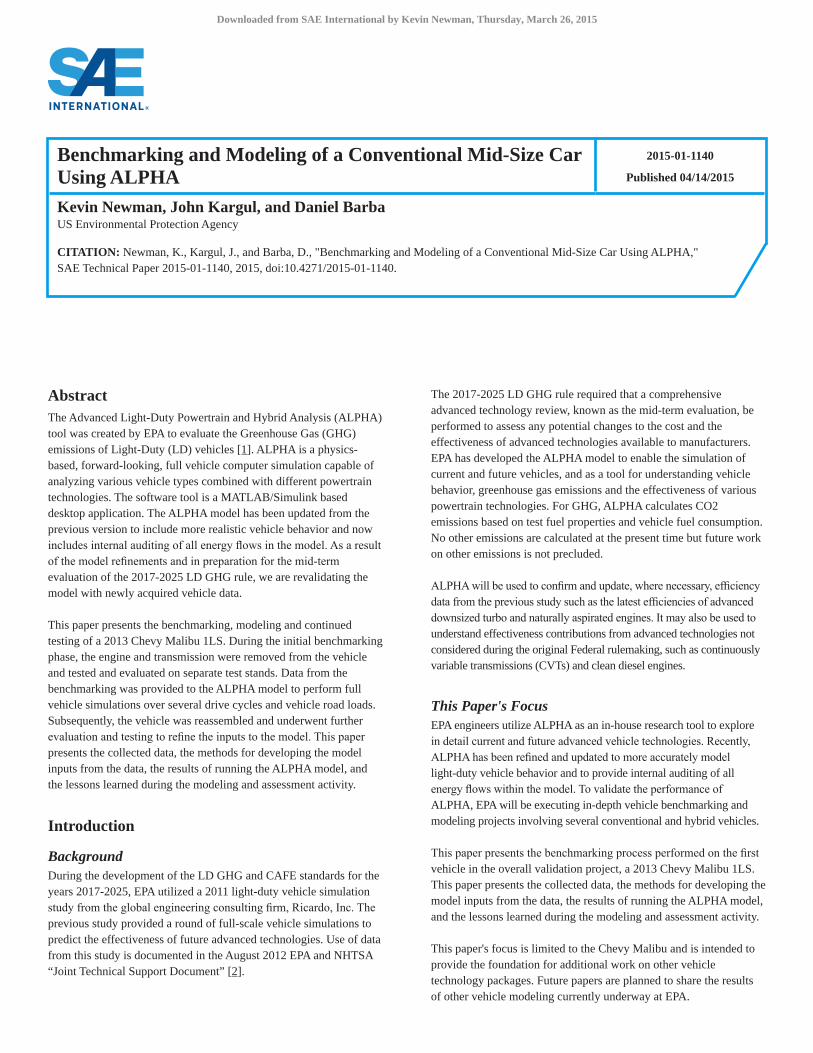
The resulting shift map is shown as a function of vehicle speed and transmission output speed (TOSS) in Figure 2.

Figure 2. Transmission shift points

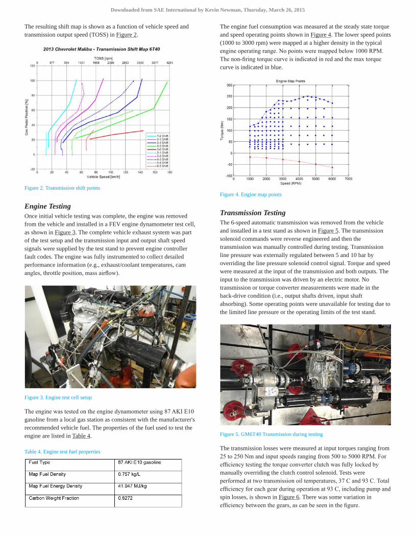
Engine TestingOnce initial vehicle testing was complete, the engine was removed from the vehicle and installed in a FEV engine dynamometer test cell, as shown in Figure 3. The complete vehicle exhaust system was part of the test setup and the transmission input and output shaft speed signals were supplied by the test stand to prevent engine controller fault codes. The engine was fully instrumented to collect detailed performance information (e.g., exhaust/coolant temperatures, cam angles, throttle position, mass airflow).

Figure 3. Engine test cell setup

The engine was tested on the engine dynamometer using 87 AKI E10 gasoline from a local gas station as consistent with the manufacturer's recommended vehicle fuel. The properties of the fuel used to test the engine are listed in Table 4.

Table 4. Engine test fuel properties

The engine fuel consumption was measured at the steady state torque and speed operating points shown in Figure 4. The lower speed points (1000 to 3000 rpm) were mapped at a higher density in the typical engine operating range. No points were mapped below 1000 RPM. The non-firing torque curve is indicated in red and the max torque curve is indicated in blue.

Figure 4. Engine map points

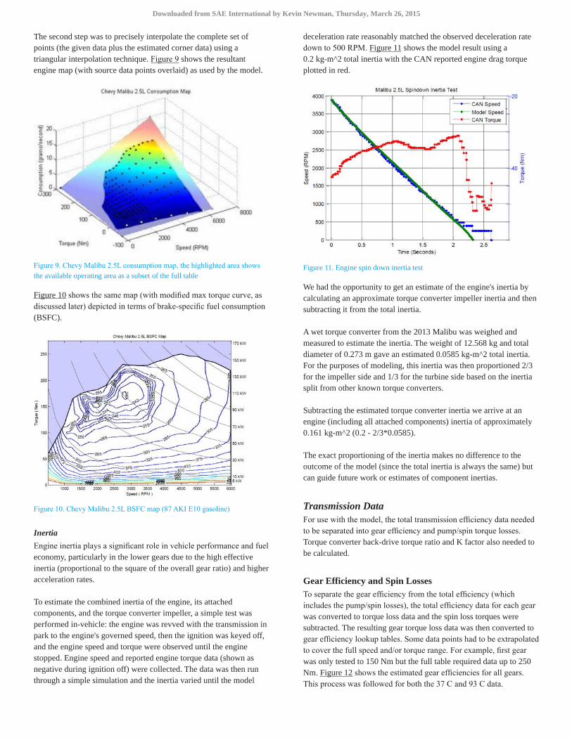
Transmission TestingThe 6-speed automatic transmission was removed from the vehicle and installed in a test stand as shown in Figure 5. The transmission solenoid commands were reverse engineered and then the transmission was manually controlled during testing. Transmission line pressure was externally regulated between 5 and 10 bar by overriding the line pressure solenoid control signal. Torque and speed were measured at the input of the transmission and both outputs. The input to the transmission was driven by an electric motor. No transmission or torque converter measurements were made in the back-drive condition (i.e., output shafts driven, input shaft absorbing). Some operating points were unavailable for testing due to the limited line pressure or the operating limits of the test stand.

Figure 5. GM6T40 Transmission during testing

The transmission losses were measured at input torques ranging from 25 to 250 Nm and input speeds ranging from 500 to 5000 RPM. For efficiency testing the torque converter clutch was fully locked by manually overriding the clutch control solenoid. Tests were performed at two transmission oil temperatures, 37 C and 93 C. Total efficiency for each gear during operation at 93 C, including pump and spin losses, is shown in Figure 6. There was some variation in efficiency between the gears, as can be seen in the figure.

Downloaded from SAE International by Kevin Newman, Thursday, March 26, 2015

Figure 6. Transmission efficiency data at 93 C and 10 bar line pressure

The torque converter was tested unlocked in 6th gear to determine speed ratio (SR), K factor and torque ratio curves. The input speed to the transmission was held at 2000 RPM while decreasing the output speed to traverse the SR curve from 1.0 to 0.35 (limited due to 10 bar line pressure and transmission slip). FEV extrapolated the data below SR 0.35 using the higher SR data. The torque converter data is shown in Figure 7, with the K factor curve normalized by dividing by the K factor at SR 0 (torque converter stall). Normalizing the K factor curve allows us to easily scale the curve up or down by multiplying by a new stall K value.

Figure 7. Torque converter torque ratio and normalized K factor versus speed ratio

Transmission spin losses were measured in each gear with a locked torque converter and no load applied to the output shaft while varying the input speed from 500 RPM to 3000 to 5000 RPM depending on the chosen gear. Spin loss testing was performed at 5 bar and 10 bar line pressures and 37 C and 93 C oil temperatures. Figure 8 shows the spin loss data at 93 C for all gears and both line pressures.

Figure 8. Transmission spin losses at 93 C

Development of Model Inputs from Benchmarking DataAfter receiving the raw data from FEV, it was necessary to adapt the data to a form suitable for use by the ALPHA model, including filling any data gaps and interpolating or extrapolating as required.

Engine DataThe default engine model in ALPHA is based on a steady-state fuel map and does not model engine thermal behavior, although a simple engine thermal model is also under development.

For use with the model, the engine's fuel consumption map was created by converting the set of points received from FEV to a rectangular surface. In addition, an estimate of the engine inertia was required since it plays a significant role in the calculation of vehicle performance and fuel economy.

Engine Fuel Consumption MapWhile constructing the engine fuel consumption map we addressed a limitation in the FEV source data set, which did not include data down the engine's idle speed (∼650 RPM). To address this limitation, an idle fuel consumption data point was added based on vehicle fuel meter data collected at EPA.

To build the map (a two-dimensional lookup table) the model requires a complete grid of data points that extends beyond the FEV supplied data. A two step process was employed to convert the engine fuel consumption data points to a rectangular grid surface map.

The first step was to loosely fit a surface through the points in order to estimate consumption at the extreme corners of the map, including expanding the overall torque and speed range slightly (so that during a simulation all the operating points lie within the generated map). At or below the non-firing engine motoring torque line, fuel consumption was set to zero.

Downloaded from SAE International by Kevin Newman, Thursday, March 26, 2015

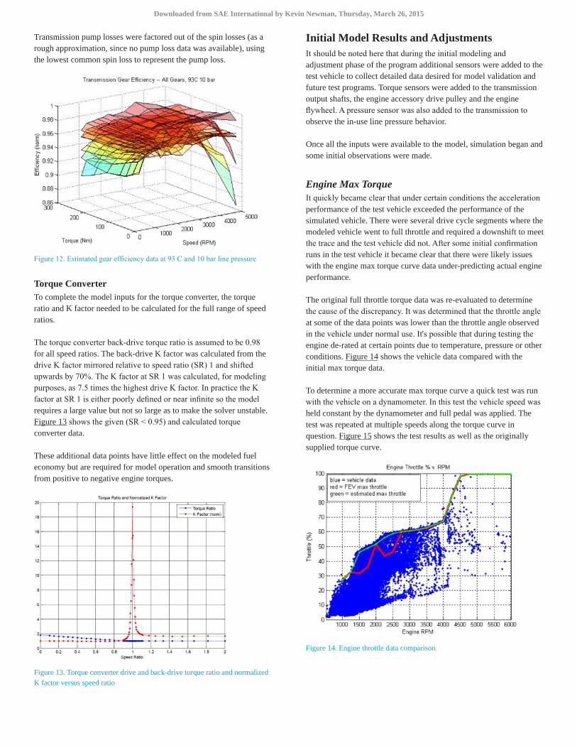
The second step was to precisely interpolate the complete set of points (the given data plus the estimated corner data) using a triangular interpolation technique. Figure 9 shows the resultant engine map (with source data points overlaid) as used by the model.

Figure 9. Chevy Malibu 2.5L consumption map, the highlighted area shows the available operating area as a subset of the full table

Figure 10 shows the same map (with modified max torque curve, as discussed later) depicted in terms of brake-specific fuel consumption (BSFC).

Figure 10. Chevy Malibu 2.5L BSFC map (87 AKI E10 gasoline)

InertiaEngine inertia plays a significant role in vehicle performance and fuel economy, particularly in the lower gears due to the high effective inertia (proportional to the square of the overall gear ratio) and higher acceleration rates.

To estimate the combined inertia of the engine, its attached components, and the torque converter impeller, a simple test was performed in-vehicle: the engine was revved with the transmission in park to the engine's governed speed, then the ignition was keyed off, and the engine speed and torque were observed until the engine stopped. Engine speed and reported engine torque data (shown as negative during ignition off) were collected. The data was then run through a simple simulation and the inertia varied until the model

deceleration rate reasonably matched the observed deceleration rate down to 500 RPM. Figure 11 shows the model result using a 0.2 kg-m^2 total inertia with the CAN reported engine drag torque plotted in red.

Figure 11. Engine spin down inertia test

We had the opportunity to get an estimate of the engine's inertia by calculating an approximate torque converter impeller inertia and then subtracting it from the total inertia.

A wet torque converter from the 2013 Malibu was weighed and measured to estimate the inertia. The weight of 12.568 kg and total diameter of 0.273 m gave an estimated 0.0585 kg-m^2 total inertia. For the purposes of modeling, this inertia was then proportioned 2/3 for the impeller side and 1/3 for the turbine side based on the inertia split from other known torque converters.

Subtracting the estimated torque converter inertia we arrive at an engine (including all attached components) inertia of approximately 0.161 kg-m^2 (0.2 - 2/3*0.0585).

The exact proportioning of the inertia makes no difference to the outcome of the model (since the total inertia is always the same) but can guide future work or estimates of component inertias.

Transmission DataFor use with the model, the total transmission efficiency data needed to be separated into gear efficiency and pump/spin torque losses. Torque converter back-drive torque ratio and K factor also needed to be calculated.

Gear Efficiency and Spin LossesTo separate the gear efficiency from the total efficiency (which includes the pump/spin losses), the total efficiency data for each gear was converted to torque loss data and the spin loss torques were subtracted. The resulting gear torque loss data was then converted to gear efficiency lookup tables. Some data points had to be extrapolated to cover the full speed and/or torque range. For example, first gear was only tested to 150 Nm but the full table required data up to 250 Nm. Figure 12 shows the estimated gear efficiencies for all gears. This process was followed for both the 37 C and 93 C data.

Downloaded from SAE International by Kevin Newman, Thursday, March 26, 2015

Transmission pump losses were factored out of the spin losses (as a rough approximation, since no pump loss data was available), using the lowest common spin loss to represent the pump loss.

Figure 12. Estimated gear efficiency data at 93 C and 10 bar line pressure

Torque ConverterTo complete the model inputs for the torque converter, the torque ratio and K factor needed to be calculated for the full range of speed ratios.

The torque converter back-drive torque ratio is assumed to be 0.98 for all speed ratios. The back-drive K factor was calculated from the drive K factor mirrored relative to speed ratio (SR) 1 and shifted upwards by 70%. The K factor at SR 1 was calculated, for modeling purposes, as 7.5 times the highest drive K factor. In practice the K factor at SR 1 is either poorly defined or near infinite so the model requires a large value but not so large as to make the solver unstable. Figure 13 shows the given (SR < 0.95) and calculated torque converter data.

These additional data points have little effect on the modeled fuel economy but are required for model operation and smooth transitions from positive to negative engine torques.

Figure 13. Torque converter drive and back-drive torque ratio and normalized K factor versus speed ratio

Initial Model Results and AdjustmentsIt should be noted here that during the initial modeling and adjustment phase of the program additional sensors were added to the test vehicle to collect detailed data desired for model validation and future test programs. Torque sensors were added to the transmission output shafts, the engine accessory drive pulley and the engine flywheel. A pressure sensor was also added to the transmission to observe the in-use line pressure behavior.

Once all the inputs were available to the model, simulation began and some initial observations were made.

Engine Max TorqueIt quickly became clear that under certain conditions the acceleration performance of the test vehicle exceeded the performance of the simulated vehicle. There were several drive cycle segments where the modeled vehicle went to full throttle and required a downshift to meet the trace and the test vehicle did not. After some initial confirmation runs in the test vehicle it became clear that there were likely issues with the engine max torque curve data under-predicting actual engine performance.

The original full throttle torque data was re-evaluated to determine the cause of the discrepancy. It was determined that the throttle angle at some of the data points was lower than the throttle angle observed in the vehicle under normal use. It's possible that during testing the engine de-rated at certain points due to temperature, pressure or other conditions. Figure 14 shows the vehicle data compared with the initial max torque data.

To determine a more accurate max torque curve a quick test was run with the vehicle on a dynamometer. In this test the vehicle speed was held constant by the dynamometer and full pedal was applied. The test was repeated at multiple speeds along the torque curve in question. Figure 15 shows the test results as well as the originally supplied torque curve.

Figure 14. Engine throttle data comparison

Downloaded from SAE International by Kevin Newman, Thursday, March 26, 2015

Figure 15. Engine max torque re-evaluation

Additionally, the questionable torque points were removed from the fuel map data set and the consumption along the new torque curve was then derived from extrapolation of the remaining points.

Transmission Line PressureDuring the model validation process it became apparent that the model was consistently underestimating the fuel economy (overestimating consumption) during high speed driving as encountered on the EPA HWFET and US06 (phase 2).

One of the missing pieces of data from the original testing was the behavior of the transmission line pressure while driving. All the transmission data was parameterized to transmission oil temperature and line pressure (5 and 10 bar) but we had no way of knowing what line pressures were applied under various conditions. We considered that possibly line pressures were lower in the higher gears than the lower gears and might explain some of the increased consumption at high vehicle speeds.

Figure 16. Transmission line pressure during vehicle operation

A line pressure sensor was added to the transmission and data were collected during vehicle operation over the various drive cycles. Figure 16 shows the collected data. The red horizontal lines are for reference at 5 and 10 bar. Interestingly line pressures were in fact relatively low in 4th and 6th gear but potentially quite high in 5th depending on load. 1st gear showed the highest line pressures with the brake pedal released and low line pressures with the brakes applied at

zero speed, presumably to reduce parasitic load on the engine at idle. In any case, it became obvious that line pressure varied dramatically depending on commanded gear and engine load. Unfortunately, without the ability to retest the transmission, it became necessary to extrapolate the transmission spin losses under certain conditions and a curve fit of line pressure versus engine torque was generated for each gear. The black lines in Figure 16 indicate the model curve fits.

High Speed Road Load

Improving the transmission line pressure model mitigated some of the discrepancy between the vehicle's high speed fuel consumption and that of the model but a significant discrepancy remained which led to an investigation of the vehicle's road load and driveline drag. Since the vehicle road load represents internal and external forces applied to the vehicle and since transmission spin losses are accounted for in the transmission model there is the possibility of “double counting” some of the transmission spin losses.

A coastdown, with the vehicle in drive, was conducted on the vehicle dynamometer and compared with the model's vehicle coastdown to determine the road load offset required to compensate for the modeled transmission drag. This is equivalent to generating “dyno set” coefficients on a vehicle dynamometer based on subtracting the vehicle's internal losses from the road load target.

Based on this testing, 2.50 N was subtracted from the road load A term and 0.750 N/m/s was subtracted from the road load B term for modeling.

Shift TableComparison of the modeled vehicle shift points and the test vehicle shift points yielded mixed results. It seemed the shift table provided reasonable results for either the mild (EPA UDDS) or aggressive (EPA US06) drive cycles but not both at the same time. The first issue with the shift table was that it was parameterized by transmission output RPM and pedal position so matching the model behavior with the vehicle's behavior required a correlation and conversion between the driver model's torque requests/pedal position and the vehicle's pedal position. With some experimentation it appeared that the vehicle's pedal position correlated well with engine power. Figure 17 shows accelerator pedal data from a US06 drive cycle that illustrates this correlation.

Figure 17. Vehicle accelerator pedal position versus (estimated) engine power

Downloaded from SAE International by Kevin Newman, Thursday, March 26, 2015

Even after remapping the model's accelerator pedal the table-based shift results were unable to model accurately the vehicle's behavior over the full range of drive cycles. Rather than spend significant time attempting to patch the table-based shift points we developed what we call an “ALPHAshift” strategy - a parametric shift algorithm that dynamically calculates transmission shift points as a function of engine fuel consumption and user defined operating limits.

A full discussion of the ALPHAshift algorithm is beyond the scope of this paper and is presented in a separate paper [3] that details the algorithm, its development, tuning and use. Figure 18 shows an example of the shift behaviors during the first phase of the EPA UDDS drive cycle.

Figure 18. Vehicle and model gear number for the beginning of the EPA UDDS drive cycle

Torque Converter LockupA cursory look at the test engine speed data revealed that the vehicle's torque converter clutch was almost always in a state of slip. Research indicates this is an NVH mitigation measure designed to avoid “chuggle” or other undesirable transmission feel [4]. ALPHA's torque converter model was updated to include the behavior of the torque converter clutch during limited slip operation, with good results as shown in Figure 19.

Figure 19. Torque converter slip during high speed cruise (US06)

Engine Idle SpeedIt was observed in the vehicle data that when coming to a stop, at about 3 MPH, the engine idle speed had an unexpected temporary flare. The model idle speed control was modified to emulate this behavior as shown in Figure 20. The effect on fuel consumption was modest but for validation purposes we chose to approximate this effect.

Figure 20. Engine idle flare at low vehicle speed, the vehicle decelerates through 3 MPH at about 551.4 seconds

Accessory LoadsThe electrical accessory load can vary considerably from test to test, according to the measured current and voltage. Figure 21 shows the measured electrical load for three of the UDDS cycles. To estimate the accessory load we calculated the average load across the 4,000 lb test data since it was the most consistent. The average was 491 Watts. The UDDS and LA92 cycles in particular show large loads during the first few minutes, presumably charging the battery after the vehicle has not been driven for some period of time (e.g., hot soak).

Figure 21. Electrical loads over the UDDS

The alternator efficiency was fixed at 66% based on vehicle data collected from the Malibu and information received from alternator suppliers. This was used to calculate the mechanical load on the engine from the electrical accessories. In addition, a fixed 50W

Downloaded from SAE International by Kevin Newman, Thursday, March 26, 2015

mechanical load was used to estimate the mechanical accessory loads, based on separate testing of the accessory drive belt with no alternator load.

Fuel Meter Data and Engine Dynamic Fuel ConsumptionA fuel meter was installed in the engine compartment and correlated to the emissions test data consumption. In this case, the meter read 96.56% of the bag emissions calculated consumption with an R-squared fit of 0.9999 across all the test data. The fuel meter data correlated well with the fuel map during steady state operation but also showed increased fuel consumption during high acceleration rates and immediately following operation with no fuel injection (“decel fuel shutoff”). Consequently, additional calculations were added to the model to provide transient fuel consumption effects not reflected in the steady state fuel map.

Figure 22 shows the effect of the acceleration-based calculation. The red line is the measured fuel rate (calculated as the derivative of the totalized fuel consumption). The blue line is the model output including the additional acceleration-based consumption, the green line is what the model output would have been based solely on the steady state fuel map. Clearly, there is variance between the two signals, highly affected as they are by driver behavior, but the added consumption closes a significant gap between the initial consumption estimate provided by the fuel map and the observed data.

Figure 22. Fuel rate with and without additional acceleration-based fuel consumption

Figure 23 shows the effect of the additional “tip-in” consumption after operating without fuel injection. The red line is the measured fuel rate, the blue line is the model output and the green is what the model output would have been based solely on the steady state fuel map. Again, there is some variation between the signals but the additional consumption helps close the gap between the steady state and observed fuel rate.

Fuel rate is particularly difficult to calibrate under dynamic conditions since it is directly affected by driver behavior and it is not possible for the model’s driver to replicate exactly the human driver’s inputs. In addition, dynamic fuel consumption effects will vary

among vehicles and powertrains and future testing is planned to quantify these effects across a range of other vehicle and powertrain technologies.

Figure 23. Fuel rate with and without additional “tip-in” fuel consumption

Model ResultsThe overall fuel economy results are shown in Figure 24 and Figure 25 for the 3,625 lb ETW and 4,000 lb ETW, respectively. The model shows good agreement with the test data. The model runs used the test data vehicle speeds as target speeds for the drive cycles to account for variations in driver behavior, as in [5].

A full discussion of model metrics and data analysis is beyond the scope of this paper, but several of the more useful comparison charts and tables are shown below as examples.

Figure 24. Test and model results for 3625 lbs ETW

The test results for the 3,625 lb ETW are shown in Table 5. The model results are within one percent of the test results.

Downloaded from SAE International by Kevin Newman, Thursday, March 26, 2015

Table 5. 3625 lbs ETW fuel economy results

Figure 25. Test and model results for 4000 lbs ETW

The test results for the 4,000 lb ETW are shown in Table 6. The model results are within three percent of the test results.

Table 6. 4000 lbs ETW fuel economy results

Figure 26. Engine speed over a sample of the UDDS

Model engine speed agrees well overall with the test vehicle engine speed, as shown in Figure 26, a natural consequence of closely matching the shift points.

Figure 27. Transmission output torques for a sample of the UDDS

The model and vehicle transmission output shaft torques are shown in Figure 27 for a portion of the UDDS and compare well with one another.

One way to factor out the second by second variability in the fuel consumption rate is the use of histograms. By using several histograms, we can compare the agreement in fuel consumption over several metrics.

Figure 28. Fuel consumption versus vehicle speed (UDDS)

A histogram of fuel consumption versus vehicle speed for the UDDS is shown in Figure 28 and there is excellent agreement between the model and test data.

Figure 29. Fuel consumption versus cycle time (UDDS)

Downloaded from SAE International by Kevin Newman, Thursday, March 26, 2015

A similar histogram of fuel consumption versus cycle time for the UDDS is shown in Figure 29 and also shows excellent agreement between the model and test data.

Figure 30. Cumulative fuel consumption (UDDS)

The cumulative fuel consumption is shown in Figure 30 and shows good agreement over the course of the drive cycle.

Summary/ConclusionsA 2013 Chevy Malibu was benchmarked at a vehicle and component level and the test data was imported into the ALPHA model.

The results of the ALPHA model simulation compared well with the results of vehicle testing at two different test weights and road loads conducted at different laboratories with different drivers (within +/− 3%).

Lessons LearnedThe process of obtaining and vetting the complete set of input data that was required to run a robust model validation provided us with many valuable insights that will be used in the future benchmarking and validation of the ALPHA model. There are a number of improvements that could be made to the data collection process that would reduce the time required to validate a vehicle and increase the robustness of the resulting model output. These improvements and observations are listed below, in approximate order of importance.

Related to Test Procedures and Methods:

• During the engine mapping process, the engine fuel consumption should be measured at idle, loaded curb idle, and zero torque at all map speeds.

• Ideally, an engine should be mapped on the engine dynamometer with the same fuel used during vehicle testing to avoid unnecessary fuel conversion factors and possible performance changes in the engine.

• Some points on the engine map seem inconsistent and may be a product of mapping test procedure. For example, observed throttle angles and loads from in-vehicle testing should be used for comparison during engine mapping.

• Based on fuel meter data, the engine's fuel consumption demonstrates dynamic effects not well modeled by the static fuel consumption map for this engine. Future testing is planned to quantify these effects across a range of other vehicle and powertrain technologies.

• Transmission efficiency as a function of temperature has been found to be a critical factor in overall vehicle fuel consumption and we will continue to gather temperature related information in future transmission benchmarking programs.

• Transmission line pressures should be observed during vehicle dynamometer tests or on-road operation before benchmarking the transmission as a standalone unit.

• Accessory loads are an important factor in fuel consumption and bear closer examination to determine if the observed variability is typical or is related to test procedure or sensor implementation.

• During the benchmarking phase of a project, it would be beneficial to determine engine and transmission inertias.

Related to ALPHA:

• The driver sub-model could use some refinement to emulate real driver behavior more realistically in the absence of actual driver vehicle speed data. The second phase of the US06 cycle seems particularly sensitive to the difference between real driver behavior and the more mathematical nature of the driver sub-model.

Next StepsWork is planned to continue improving our vehicle and engine benchmarking methods and refining the ALPHA model with additional advanced technology validations.

For examples of other recent and related vehicle modeling and testing work, see [6,7,8].

References1. Lee, B., Lee, S., Cherry, J., Neam, A. et al., “Development of

Advanced Light-Duty Powertrain and Hybrid Analysis Tool,” SAE Technical Paper 2013-01-0808, 2013, doi:10.4271/2013-01-0808.

2. US EPA, DOT/NHTSA, “Final Rulemaking to Establish Light-Duty Vehicle Greenhouse Gas Emission Standards and Corporate Average Fuel Economy Standards, Joint Technical Support Document,” http://www.epa.gov/otaq/climate/regulations/420r10901.pdf, Aug. 2012

3. Newman, K., Kargul, J., and Barba, D., “Development and Testing of an Automatic Transmission Shift Schedule Algorithm for Vehicle Simulation,” SAE Technical Paper 2015-01-1142, 2015, doi:10.4271/2015-01-1142.

4. MSC Software, “Automotive Chuggle Simulation Using ADAMS,” http://support.mscsoftware.com/cgi-bin/kb_files/GM_Chuggle_2001_NAUC.pdf?name=ri%2F1-13%2F1-13B2-2141%2FGM_Chuggle_2001_NAUC.pdf

5. Meng, Y., Jennings, M., Tsou, P., Brigham, D. et al., “Test Correlation Framework for Hybrid Electric Vehicle System Model,” SAE Int. J. Engines 4(1):1046-1057, 2011, doi:10.4271/2011-01-0881.

6. Moskalik, A., Dekraker, P., Kargul, J., and Barba, D., “Vehicle Component Benchmarking Using a Chassis Dynamometer,” SAE Technical Paper 2015-01-0589, 2015, doi:10.4271/2015-01-0589.

Downloaded from SAE International by Kevin Newman, Thursday, March 26, 2015

7. Stuhldreher, M., Schenk, C., Brakora, J., Hawkins, D. et al., “Downsized boosted engine benchmarking method and results,” SAE Technical Paper 2015-01-1266, 2015, doi:10.4271/2015-01-1266.

8. Safoutin, M., Cherry, J., McDonald, J., and Lee, S., “Effect of Current and SOC on Round-Trip Energy Efficiency of a Lithium-Iron Phosphate (LiFePO4) Battery Pack,” SAE Technical Paper 2015-01-1186, 2015, doi:10.4271/2015-01-1186.

Contact InformationKevin Newman, M.Eng.National Center for Advanced TechnologyUS EPA - Office of Transportation & Air Qualitynewman.kevin@epa.gov

AcknowledgmentsThe author would like to thank Thomas D'Anna, Clay Cooper and Neal Persaud of FEV for taking the time to answer technical questions regarding their testing and evaluation of the Chevy Malibu.

On February 3, 2015, subject matter experts from GM's Global Energy Analysis, Execution and Tools team and GM's Public Policy Center team met with EPA to discuss technical work associated with the near final draft of this SAE paper. In general, GM subject matter experts thought that the work and analysis was directionally correct. GM had constructive comments on many key aspects of the analysis with special emphasis on EPA's application of dynamic fuel rate calculations to account for additional fuel used during transient engine operation. GM cautioned that dynamic fuel effects are very application and technology specific, and that appropriate methods to estimate these effects will be required when modeling other engine/vehicle configurations. GM also emphasized that the inappropriate use of dynamic fuel rate calculations may confound comparisons of component and subsystem efficiencies among different vehicles. We appreciate GM's valuable input as we further enhance the ALPHA model.

Definitions/AbbreviationsALPHA - Advanced Light-Duty Powertrain and Hybrid Analysis modeling tool

UDDS - US EPA Urban Dynamometer Driving Schedule

HWFET - US EPA Highway Fuel Economy Test

LA92 - CARB California Unified Cycle (UC) or CARB Unified Cycle Driving Schedule (UCDS)

ETW - Equivalent Test Weight

CARB - California Air Resources Board

NVH - Noise, Vibration, and Harshness

chuggle - vehicle longitudinal vibration caused by an excited torsional transmission/driveline mode under torque converter quasi-lock-up conditions

The Engineering Meetings Board has approved this paper for publication. It has successfully completed SAE's peer review process under the supervision of the session organizer. This process requires a minimum of three (3) reviews by industry experts.

This is a work of a Government and is not subject to copyright protection. Foreign copyrights may apply. The Government under which this paper was written assumes no liability or responsibility for the contents of this paper or the use of this paper, nor is it endorsing any manufacturers, products, or services cited herein and any trade name that may appear in the paper has been included only because it is essential to the contents of the paper.

Positions and opinions advanced in this paper are those of the author(s) and not necessarily those of SAE International. The author is solely responsible for the content of the paper.

ISSN 0148-7191

http://papers.sae.org/2015-01-1140

Downloaded from SAE International by Kevin Newman, Thursday, March 26, 2015