Belief Updating and the Demand for Information

Sandro Ambuehl∗and Shengwu Li†

July 2, 2014

Abstract

How do individuals value noisy information that guides economic decisions?

Using a novel laboratory experiment, we investigate the willingness-to-pay for

useful information. We identify two systematic biases in information demand.

Compared to the standard rational agent model, individuals over-value low

quality information and under-value high quality information. They also dis-

proportionately prefer information that may yield certainty. By eliciting agents’

posterior beliefs, we find that both these biases are well-explained by non-

Bayesian belief updating. Furthermore, individuals differ consistently in their

responsiveness to information - the extent that their beliefs move upon observ-

ing signals. This single trait explains about 80% of the variation in information

demand that is attributable to belief updating. It is also predictive of behav-

ior across different choice environments. Thus, we find that the demand for

information is driven by belief updating, and that belief updating behavior is

a stable individual trait.

JEL classification: C91, D01, D03, D83

Keywords : Demand for information, belief updating, responsiveness to informa-

tion, experimental economics

∗sambuehl@stanford.edu†shengwu@stanford.edu. Both authors are at Stanford University, Department of Economics,

Landau Economics Building, 579 Serra Mall, Stanford, CA, 94305. We are deeply indebted to

our advisors B. Douglas Bernheim, Paul Milgrom, Muriel Niederle, Alvin E. Roth, and Charles

Sprenger. We are grateful to Itay Fainmesser, Simon Gaechter, Mark Machina, Jeffrey Naecker

and participants at the Stanford Behavioral and Experimental Economics Lunch for very helpful

comments and discussions. Financial support for this project was provided by the Department of

Economics at Stanford University.

1

Contents

1 Introduction 3

1.1 Related Literature . . . . . . . . . . . . . . . . . . . . . . . . . . . . 7

2 Experimental Design 10

2.1 Setup . . . . . . . . . . . . . . . . . . . . . . . . . . . . . . . . . . . . 10

2.2 Research Questions . . . . . . . . . . . . . . . . . . . . . . . . . . . . 12

2.3 Implementation . . . . . . . . . . . . . . . . . . . . . . . . . . . . . . 15

3 Preliminary Analysis 20

4 Demand for Information 22

4.1 Is the demand for information driven by belief updating? . . . . . . . 25

5 Consistent Individual Heterogeneity 28

5.1 Are individuals consistent within tasks? . . . . . . . . . . . . . . . . . 29

5.2 A structural model of responsiveness to information. . . . . . . . . . . 30

5.3 Are individuals consistent across tasks? . . . . . . . . . . . . . . . . . 32

5.4 Out-of-sample test: The Gradual Information Task . . . . . . . . . . 35

6 Discussion 41

7 Concluding Remarks 43

A Correlates of Responsiveness to Information 51

B Robustness Checks 55

B.1 Analysis on the full sample . . . . . . . . . . . . . . . . . . . . . . . . 55

B.2 Truncation in the aggregate analysis . . . . . . . . . . . . . . . . . . 60

B.3 Framing effects and extremeness-avoidance . . . . . . . . . . . . . . . 60

B.4 Responsiveness and subsets of information structures . . . . . . . . . 63

C Responsiveness to Information Compared to Risk Aversion 63

D Experimental Instructions 66

2

1 Introduction

Modern economies increasingly trade not just in physical goods, but in information.

Economic agents consider whether to purchase medical tests, consulting expertise,

or financial forecasts. Entire industries are premised on the sale of useful but noisy

information.

However, the demand for useful information is not like the demand for coffee or

convertibles; it is not a brute fact arising from inarguable tastes. Rather, the standard

rational agent model tightly predicts agents’ demand for information: Agents foresee

that they will update prior beliefs according to Bayes’ Law, they foresee what decisions

they will make after each possible signal realization, and they evaluate the resulting

lottery over outcomes. Hence, agents’ willingness to pay for information will be

entirely determined by the properties of the signal, their prior beliefs, and their risk

preferences. These predictions have not yet been thoroughly examined. (We will

review the literature shortly.)

In this paper, we use a laboratory experiment to systematically investigate the

behavioral properties of the demand for information. Our experiment uses modifica-

tions of familiar urns-and-balls tasks. In these tasks, subjects receive signals about a

payoff-relevant ‘state of the world’ with a known state-contingent signal distribution.

This signal distribution is implemented by drawing colored balls from a virtual urn,

with a different urn for each state. In our setting, information is stochastic, instru-

mentally useful,1 and has no intrinsic value.2 Strategic considerations play no role,

and by design, concavity of the utility function cannot affect behavior.3

We use a laboratory experiment because this gives us precise control over prior

beliefs and signal distributions, allowing us to identify behavior in ways that are not

1As opposed to studies in which the same action will or should be taken regardless the outcomeof the informative signal, such as in Bastardi and Shafir (1998) and Eliaz and Schotter (2010).

2As opposed to studies in which subjects arguably derive utility from their beliefs, such as Burkset al. (2013), Eil and Rao (2011), Ertac (2011), and Moebius et al. (2013).

3We achieve this by letting subjects earn one of only two possible amounts for participation inthe experiment.

3

possible with field data.

Our experiment first elicits subjects’ willingness-to-pay (WTP) for a set of pos-

sible signals, and later elicits subjects’ posterior beliefs conditional on each signal

realization. There are thus two ways to assess biases in the demand for information:

Subjects may be biased relative to the objective Bayes posteriors, or subjects may be

biased relative to their own posterior beliefs.

When we compare subjects’ WTP to the objective Bayesian benchmark, we iden-

tify two biases in the demand for information. First, subjects’ willingness-to-pay for

low-quality information is too high, and their willingness-to-pay for high-quality in-

formation is too low.4 Second, subjects disproportionately prefer information that

may yield certainty about the state of the world.5 (We also consider the hypothesis

that subjects prefer ‘symmetric’ information whose quality does not depend on the

state of the world, but do not find evidence for this hypothesis.6)

These biases may either arise because of subjects’ non-standard belief updating,

or because of non-standard valuations of information even conditional on beliefs.7

For instance, subjects may desire certainty because they are averse to making choices

that have even the possibility of error. By comparing subjects’ elicited WTP to the

WTP implied by their own posterior beliefs, we can decompose the biases into a

part that is due to biased belief updating, and a remainder.8 We find that the two

4This first bias is reminiscent of the system neglect hypothesis in Massey and Wu (2005).5This is consistent with results by Andreoni and Sprenger (2012), Andreoni and Sprenger (2013),

Gneezy et al. (2006), Keren and Willemsen (2008), Rydval et al. (2009), Simonsohn (2009), whosuggest that subjects have a disproportionate preference for certainty in choice from single-stagelotteries.

6This is contrary to what recent experimental and theoretical literature of decision making underuncertainty suggests. (Ergin and Gul (2009), Halevy (2007), Halevy and Feltkamp (2005), Seo(2009), Yates and Zukowski (1976), Bernasconi and Loomes (1992))

7There are two other factors which, in principle, may cause these biases. First, agents may failto correctly foresee what action they will choose after obtaining a particular piece of information.Second, agents may entertain incorrect assessments of the probability of receiving a particular pieceof information. In our experiment, subjects exhibit neither of these failures systematically.

8This exercise, however, does not decompose behavior into beliefs and preferences. In the subjec-tive expected utility framework, preferences are basic, and beliefs are just part of the representation.(Savage (1954)) To be scrupulous, when we say that a subject deviates from Bayesian belief updat-ing, we mean “in the representation that rationalizes this choice, the beliefs differ from the objective

4

previous biases disappear – they are wholly driven by non-standard belief updating.

However, we identify a third bias: Conditional on their own posterior beliefs, subjects’

willingness-to-pay for information is too low.

Given the importance of non-standard belief updating in determining the demand

for information, we then investigate individual heterogeneity in belief updating. Pre-

vious research may suggest that subjects’ belief updating behavior is essentially a

noisy version of Bayesian updating – apart from some aggregate tendencies such as

conservatism (Peterson and Beach (1967)) or base-rate neglect (Kahneman and Tver-

sky (1974)).

By contrast, we identify a new dimension of systematic variation. Subjects’ re-

sponsiveness to information – the extent that beliefs move upon observing signals –

is a stable and predictive individual trait: A subject who, in some cases, updates

beliefs too conservatively (or not conservatively enough) tends to do so in all cases,

and by comparable amounts. This trait is orthogonal to measures of mathematical

aptitude, such as college major and self-reported knowledge of Bayes’ Law.

We parametrically estimate subjects’ responsiveness to information in one task,

and thus predict their behavior in other tasks. We find that subjects who update

beliefs too conservatively have too low a willingness-to-pay for information, and sub-

jects who update beliefs too much have too high a willingness-to-pay for information.

In fact, responsiveness to information is by far the most important component of non-

Bayesian belief updating in our experiment. For each subject, we use a one-parameter

model of responsiveness to predict willingness-to-pay in ten different choice problems.

The model explains about 20% of the individual variation in willingness-to-pay. This

is about 80% of the total variation that can be explained by belief updating when we

use an unconstrained procedure.

To buttress our case that responsiveness to information is a consistent individual

trait, we perform a further test using a different choice environment. Subjects obtain

Bayes posteriors.”

5

noisy information about a binary state of the world in a piecemeal fashion, and decide,

after each piece of information, whether to take an exogenous lottery or to bet on the

state of the world. Consistent with our hypothesis, subjects who are more responsive

to information require less information before placing a bet on the state of the world.

Thus, individual responsiveness is significantly correlated across three distinct choice

environments.

We suggest some important implications of these results.

Our finding that subjects overvalue low-quality information and undervalue high

quality information suggests that sellers of information may wish to split information

in many smaller chunks rather than selling it as a whole.9 The finding that subjects

have a disproportionate preference for information that may eliminate all uncertainty

implies that it is profitable for sellers of information to (appear to) be able to provide

information that is perfect in at least some of the states of the world.

Our results on consistent heterogeneity in responsiveness to information constitute

a direct answer to one of the abiding puzzles in financial theory, the Milgrom-Stokey

no-trade theorem (Milgrom and Stokey (1982)). This theorem roughly states that so-

phisticated agents starting from a Pareto efficient allocation will not exchange bets on

payoff-relevant events once they receive private information.10 The no-trade theorem

fails to hold when agents are heterogenous in their responsiveness to information, even

when agents’ responsiveness to information is common knowledge. Hence, consistent

heterogeneity in responsiveness can explain why financial trades occur in equilibrium

between strategically sophisticated agents.

9Koszegi and Rabin (2009) develop a model which implies that decision-makers are averse toreceiving information piecewise. However, our findings are supported by an experiment conductedby Zimmermann (2014), who finds that individuals do not have a preference against piecewiseinformation.

10The theorem states that if a market with risk-averse traders with rational expectations startsin a Pareto optimal allocation (relative to traders’ prior beliefs), and traders receive private infor-mation, then traders will not exchange bets on payoff-relevant events. In particular, this result doesnot require the assumption of common priors, only a condition which roughly means that tradersagree about how instrumentally useful information should be interpreted: Beliefs are required to beconcordant.

6

Heterogeneity in responsiveness to information could also explain excessive price

volatility in financial markets, as investigated by Shiller (1981). In competitive finan-

cial markets, stock prices are determined by the marginal investor. If, in equilibrium,

marginal investors have more extreme beliefs about returns than the average agent

in the market, then marginal investors are also likely to be more responsive to infor-

mation than the Bayesian norm. This is a channel that could amplify price volatility

in response to information shocks.

If, moreover, the identification of individuals who are more responsive to informa-

tion is possible, the targeting of programs such as those intended to foster technology

adoption in developing countries may be improved.

Finally, in settings where non-Bayesian updating is costly, such as medical decision

making, subjects who are over- or under- responsive to information might be identified

and given help to bring their decision-making in line with the normative benchmark.

1.1 Related Literature

Demand for Information Hoffman (2012) is the study most closely related to

ours. Hoffman conducts a field experiment investigating internet domain name traders’

willingness to pay for stochastic information. He finds the expected comparative stat-

ics: willingness to pay increases with the accuracy of the information, and decreases

with the extremeness of the prior of the subject. Similar to one of our results, Hoffman

finds that willingness to pay for information falls short of a normative benchmark.

Puzzlingly, Hoffman also finds that about a third of his subjects who purchase infor-

mation do not use it.11

Our study differs from Hoffman’s on many dimensions. Most importantly, we

investigate how behavioral biases depend on the properties of the information struc-

tures, and we demonstrate that responsiveness to information is an important ex-

11Subjects in Hoffman’s experiment make decisions that mimick those they engage in in theirprofessional lives. Hence, subjects beliefs are possibly ego-relevant, which might influence some ofHoffman’s results.

7

planatory factor of the demand for information.

The remaining research that empirically studies the demand for information in

non-strategic settings either considers information of a kind that should not change

individuals’ actions, investigates demand for explicitly ego-relevant information, or

studies preferences concerning the resolution of uncertainty over time.

Eliaz and Schotter (2010) and Bastardi and Shafir (1998) study the demand

for non-instrumental information. Eliaz and Schotter’s subjects exhibit a positive

willingness-to-pay for information if this information makes them more confident

that they have chosen the right action, even when this information would not af-

fect their decisions. Bastardi and Shafir use an across-subjects design to show that

non-instrumental information structures may influence subjects’ behavior if they ac-

tively decide to wait for the arrival of this information. Subjects in the treatment

group who decided to pursue information tended to base their actions on the signal

realizations, even though subjects in the control group stated that they would take

the same action regardless of the signal realization.

The studies considering ego-relevant information (Burks et al. (2013), Eil and Rao

(2011), and Moebius et al. (2013)) typically find that subjects’ willingness-to-pay for

information increases the more confident the subject is that the desirable state of the

world obtains.12

The results about preferences for the resolution of uncertainty over time are more

mixed. Zimmermann (2014) tests Koszegi and Rabin (2009)’s prediction that individ-

uals are averse to receiving information in a piecemeal fashion, and finds no support

for this hypothesis. On the other hand, Kocher et al. (2009) find that subjects holding

a lottery ticket have a preference for delayed resolution of risk, and that this effect is

driven by anticipatory utility.

The valuation of – and hence demand for – information in non-strategic settings

has also been the topic of recent interest in the theoretical literature. Azrieli and

12In these studies, subjects are not asked to make any decisions after they learn the informationthey purchased.

8

Lehrer (2008) consider the set of functions that map an information structure into

a valuation and provide a characterization of the subset of such functions that is

consistent with Bayesian updating and expected utility. Athey and Levin (2001)

study Bayesian updaters’ demand for information in monotone decision problems;

and Cabrales et al. (2013a) and Cabrales et al. (2013b) derive settings in which

information structures can be totally ordered by the reduction in the entropy of

beliefs they afford. Our experiment lends partial support to the assumption that the

valuation of information is well approximated by the Bayesian benchmark, but does

not directly address this theoretical literature.

Belief Updating A recent literature demonstrates the importance of studying be-

lief updating by showing that beliefs causally affect economic behavior. Costa-Gomes

et al. (2012) investigate behavior in a trust game. These authors use an instrumen-

tal variable approach to show that a trustor’s beliefs about the level of re-payment

causally affect how much she transfers to the trustee. Our work establishes that

beliefs causally affect information demand behavior.

Heterogeneity in belief updating that is consistent within individuals has also been

observed (but not explicitly investigated) in Peterson et al. (1965). These authors

conducted a non-incentivized urns-and-balls experiment and observed that individ-

uals who updated more conservatively than others in some tasks also tended to do

so in closely related tasks. More recently, Augenblick and Rabin (2013) analyze a

dataset on dynamic individual beliefs about geopolitical events, and show that if a

forecaster’s belief stream for a given geopolitical event exhibits much movement, then

the same forecaster’s belief streams for other events also tend to exhibit much move-

ment. Relatedly, Moebius et al. (2013) rank divide their subjects into two groups

of more and less conservative updaters. They show that for both groups measured

posteriors about ability are equally predictive of a decision to enter a tournament

that depends on ability. This suggests that conservative types of high ability take

9

too few risks while conservative types of low ability take too many risks, a prediction

that receives support in Moebius et al.’s data.13

Our experiment more generally relates to the vast literature on belief updating

(see Camerer (1995) for a review). The earlier papers in this literature conclude that

Bayesian updating is a viable description of human belief updating, with the exception

that humans tend to update more conservatively than Bayesian subjects would (see

Peterson and Beach (1967) for a review).14 Our experiment lends some support to the

idea that subjects’ behavior is reasonably well approximated by Bayesian updating,

although we find little evidence of conservatism in belief updating for the average

subject. The more recent papers in the literature on belief updating focus on non-

Bayesian tendencies such as the representativeness heuristic (Kahneman and Tversky

(1972), Grether (1980)). We designed our experiment to minimize the salience of

such heuristics.

2 Experimental Design

2.1 Setup

We consider a setting in which information is valuable (solely) because it informs a

subsequent choice. We focus on the simplest nontrivial such setting, which we call

the prediction game. There is a binary state of the world s ∈ {0, 1}. An agent

has an objective prior belief P (s = 1) = 12. The agent then observes a realization

σ ∈ {“0”, “1”} of a stochastic signal before he makes a guess g concerning which of

the states of the world obtains. The agent obtains a prize k > 0 if he guesses correctly,

and 0 if he doesn’t. Importantly, the agent is aware of the pair of state-dependent

probabilities PI(σ = “1”|s = 1) and PI(σ = “0”|s = 0) of each signal realization. We

13Moebius et al. (2013) use exogenous random variation in the signal realizations as an instrumentto establish causality.

14Additionally, Benjamin et al. (2013) contains a comprehensive review the literature on beliefupdating experiments that use binary states and binary signals.

10

denote the events {σ = “1”} and {s = 1} by “1” and 1, respectively, and abbreviate

the 0-signal and the 0-state similarly.

We refer to a pair I =(PI(“1”|1), PI(“0”|0)

)as an information structure.15 This

information is sufficient for the agent to be able to employ Bayes’ Law to inform his

guess about the state of the world.

We elicit agents’ willingness-to-pay to play the prediction game, by asking for

incentivized reports of their uncertainty equivalents. That is, we ask what probabil-

ity vI,i leaves agent i indifferent between (i) the lottery that pays the prize k with

probability vI,i and 0 otherwise, and (ii) participating in the prediction game with

information structure I.16 This measure of willingness-to-pay rules out confounds

from wealth effects and classical risk aversion.17 Henceforth, we refer to vI,i as agent

i’s valuation of information structure I.18

Even if we consider an agent who is not a Bayesian expected utility maximizer,

we can use the agent’s subjective posterior beliefs PI,i(σ|“σ”) and signal probability

assessments PI,i(“σ”) to predict this agent’s valuation of information structure I —

provided the agent (i) reduces compound lotteries, (ii) has preferences that depend

only on final outcomes, and (iii) strictly prefers obtaining the prize k to not obtaining

it. To assess his valuation of an information structure, such an agent first devises

a strategy g(“σ”) mapping each possible signal realization into a guess about the

state of the world. He then considers the probability PI,i(g(“σ”)|“σ”

)with which he

will guess the state of the world correctly after each signal realization “σ”. Finally,

15It is apparent that in our setting an information structure in the sense of Azrieli and Lehrer(2008) is fully described by a pair of probabilities.

16Note that since vI,i is a lottery between the best and worst monetary outcomes in this setting, ifthe agent agent’s preferences admit an expected utility representation, vI,i is precisely the expectedutility of the prediction game.

17Under the assumptions of expected utility theory, agents’ preferences over lotteries are linearin probabilities (holding outcomes fixed). Thus, per Roth and Malouf (1979), payment proceduresemploying such two-outcome lotteries induce choice behavior that does not depend on the particularsof the Von Neumann-Morgenstern utility function.

18If the signals were completely uninformative, the agent would have a 0.5 chance of winning theprize by guessing. vI,i − 0.5 can thus be interpreted as the value that the agent places on observinga signal drawn from I.

11

he takes the expectation of these probabilities with respect to the signal realization

probabilities PI,i(“σ”). Hence, his valuation of information structure I is given by

vI,i = PI,i(g(“1”)|“1”

)PI,i(“1”) + PI,i

(g(“0”)|“0”

)PI,i(“0”). (1)

Our experiment is designed to elicit each constituent part of equation (1). In the

information valuation task, we present subjects with ten different information struc-

tures, and elicit their valuations vI,i for each of them. In the belief updating task, we

elicit subjects’ subjective posterior probabilities PI,i(σ|“σ”) and in the signal proba-

bility assessment task, we obtain the subjects’ assessment of the probability PI,i(“σ”)

of observing a given signal realization “σ”. The details of the implementation are

discussed in section 2.3.

2.2 Research Questions

How would a classical agent behave in our setting? In our setting, an information

structure is a pair of probabilities, I =(PI(“1”|1), PI(“0”|0)

). Hence, the space of

all information structures is the unit square [0, 1] × [0, 1]. Our experiment focuses

on the subspace [0.5, 1] × [0.5, 1]. For information structures in this subspace, the

optimal guessing strategy is to follow the signal, g(“σ”) = σ. Using this, and re-

placing the subjective probabilities PI,i(σ|“σ”) and PI,i(“1”) in equation (1) by their

objective (Bayesian) counterparts, we obtain the valuation of information structure

I as predicted by the standard model19

vtheorI =PI(“1”|1) + PI(“0”|0)

2(2)

19There is another way of obtaining this expression: The agent’s optimal strategy is to guess s = 1after signal “1”, and to guess s = 0 after signal “0”. Consequently, the probability that the agentguesses correctly is the sum of the probability that signal “1” realizes and the state is 1 and theprobability that signal “0” realizes and the state is 0. Together with the fact that P (s = 1) = 1

2 weobtain the stated expression.

12

InformativenessAsymmetry

.5.6

.7.8

.91

P("1"|1)

.5 .6 .7 .8 .9 1P("0"|0)

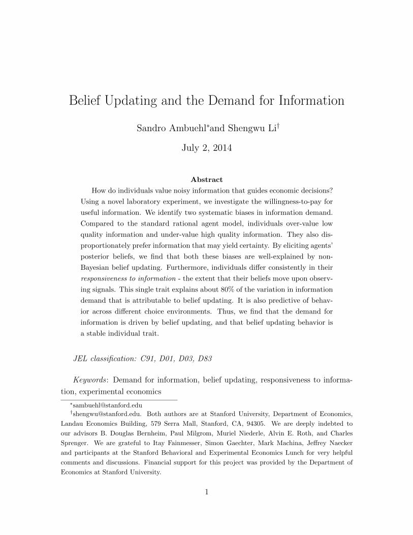
Figure 1: The set [0.5, 1] × [0.5, 1] of information structures and the level curves ofvtheorI . If information structure I ′ lies to the northeast of I, then I ′ is more informativethan I. If I ′ lies to the northwest of I, then I ′ is more asymmetric than I.

Figure 1 displays the set of information structures I ∈ [0.5, 1] × [0.5, 1] and the

level curves of vtheorI . We refer to vtheorI as the informativeness of information structure

I; this is the probability that the signal matches the state of the world. We refer to

the orthogonal dimension as asymmetry.

Empirically, valuations of information structures may differ from the Bayesian

predictions for three reasons.

First, a literature on belief updating (Massey and Wu (2005), Fiedler and Juslin

(2006)) has found that subjects’ updates do not always take the properties of infor-

mation structures into account to a sufficiently large degree. If a similar hypothesis

holds for the valuation of information structures, we expect to find valuations that

vary insufficiently with the informativeness of the information structures.

Second, the literature of decision making under risk (Andreoni and Sprenger

(2012), Andreoni and Sprenger (2013), Gneezy et al. (2006), Keren and Willemsen

(2008), Rydval et al. (2009), Simonsohn (2009)) finds that subjects have a dispro-

portionate preference for certainty.20 We therefore hypothesize that subjects will

20In Andreoni and Sprenger (2013) subjects comparing pairs of two-outcome lotteries. 38% of

13

have disproportionately high values for information structures where at least one sig-

nal realization yields certainty. These are the lotteries on the northern and eastern

boundaries of Figure 1.

Third, a recent theoretical and experimental literature suggests that subjects dis-

like spreads in the first-stage distribution of two-stage lotteries that leave total success

probability constant. (Ergin and Gul (2009), Halevy (2007), Halevy and Feltkamp

(2005), Seo (2009), Yates and Zukowski (1976), Bernasconi and Loomes (1992)) We

therefore hypothesize that subjects will, ceteris paribus, place higher value on more

symmetric information structures. This implies that the indifference curves in Figure

1 will instead be convex.

Our experiment is designed to test for these three biases in the demand for infor-

mation, by presenting subjects with a variety of information structures and eliciting

their willingness-to-pay for information. We then elicit subjects’ posterior beliefs, and

investigate whether these biases in the demand for information can be explained by

non-Bayesian belief updating.

Our data confirm the first two hypotheses. Individual valuations vary insuffi-

ciently with the informativeness of the information structures, and subjects have a

disproportionate preference for boundary information structures. We find no evi-

dence of a preference for symmetric information structures. Using subjects’ elicited

posterior beliefs, we find that biases in information valuation are well explained by

non-Bayesian belief updating.

We conjecture that subjects will exhibit consistent individual heterogeneity when

updating beliefs. In particular, we hypothesize that individuals have heterogeneous

responsiveness to information: Some individuals’ beliefs move more in response to

evidence than is warranted by Bayes’ Law, and some individuals’ beliefs move less.

We investigate whether responsiveness is consistent ; that is, whether a given subject

exhibits similar responsiveness across different choice problems.

their subjects even exhibit preferences for certainty that violate stochastic dominance.

14

Our data confirm that subjects’ responsiveness to information is consistent both

within and across choice environments. Individual choices are highly correlated within

each choice environment. An individual’s responsiveness, as estimated in one choice

environment, significantly predicts their behavior in two other choice environments.

In particular, the relationship between belief updating and information valuation is

substantially captured by a simple model of responsiveness.

2.3 Implementation

We implemented the experiment on computers using variations of familiar urns-and-

balls tasks. In each part of the experiment, subjects faced pairs of boxes filled with

black and white balls. We distributed and read aloud the instructions directly before

each part and (correctly) informed subjects that their choices in any part would not

affect their earnings from any other part.

Subjects received no feedback as to the outcomes of their choices in any part of

the experiment until the experiment was concluded. At the end of the experiment,

the computer selected a random part and a random decision within that part for

payment so that subjects had monetary incentives to answer each of our questions

truthfully. The experiment proceeded in five parts, as follows:

Part 1: Prediction Game Part 1 of the experiment was intended to familiarize

subjects with the prediction game that they would subsequently be asked to value.

In this part, each subject played six rounds of the prediction game. Subjects were

presented with two boxes, Box X and Box Y. Box X contained 10 balls, the majority

of which were black. Box Y contained 20 balls, the majority of which were white.

15

PART 1

The first part of the experiment proceeds in 6 rounds. In each round, you will play the Prediction Game (described below), for a prize of $35. In each round there are two boxes, Box X and Box Y. Each of the boxes contains balls that are either black or white. Box X contains 10 balls. Box Y contains 20 balls. For example, Box X could contain 7 black balls and 3 white balls, and Box Y could contain 14 white balls and 6 black balls. The composition of the boxes may change from round to round.

THE PREDICTION GAME At the beginning of the Prediction Game, the computer will select either Box X or Box Y by tossing a fair coin. Thus, Box X is selected with chance 50%, and Box Y is selected with chance 50%. The box that has been selected is called the Selected Box. We will not tell you which box has been selected by the computer.

The computer will then draw a ball randomly from the Selected Box, and show that ball to you. Your task is to predict whether the Selected Box is Box X or Box Y. If you predict correctly, you will receive $35. If you predict incorrectly, you will receive $0.

The subject observed the contents of the boxes, in the manner shown by the

screenshot above. The computer then randomly (and secretly) selected a box, each

with 50% probability, and showed the subject a ball drawn at random from that

box. The subject then guessed which box was selected, receiving $35 if she guessed

correctly, and $0 otherwise. Subjects played the prediction game for six different

information structures.21 The box selected corresponds to the state of the world s,

while the color of the ball drawn corresponds to the signal realization “σ”.

Part 2: Information Valuation Task Part 2 of the experiment was designed

to elicit subjects’ valuations of information structures vI,i. Subjects were presented

with 10 different pairs of boxes, corresponding to the information structures depicted

in figure 2. We chose the information structures so as to be able to easily test for

preferences about symmetry and certainty.22 For each pair of boxes, subjects were

asked to report their uncertainty equivalents for playing the Prediction Game with

those pairs of boxes. Subjects made their choices by filling in a multiple price list (a

Becker-deGroot-Marschak mechanism), choosing between pairs of options: “Play the

21We drew the colors of the balls conditionally i.i.d. random for each subject. The informationstructures used were {(0.5, 0.9), (0.7, 1), (0.6, 0.6), (1, 0.55), (0.6, 0.85), (0.8, 0.6)}. We used six infor-mation structures so that each subject would be quite likely to see both black and white draws, butalso so that this part of the experiment would be concluded quickly.

22We had initially planned to conduct a subject-by-subject analysis of the shape of the utilityfunction using the non-parametric test for convexity by Abrevaya and Jiang (2005). The set ofinformation structures we chose also partially reflects simulated power calculations for this test. Wedo not perform this analysis since after obtaining our data we discovered that Abrevaya and Jiang’stest is subject to considerable bias with small sample sizes.

16

Prediction Game” or “Win $35 with chance p”, for p between 1% and 100%, in 3%

intervals.23 Subjects were informed that if the current round was randomly chosen

for payment, a random line from the price list would be selected, and their decision

on that line would be carried out. Hence, truthful revelation was strictly optimal

for subjects.24 We constrained subjects to have at most one switching point.25 Half

the subjects, chosen at random, evaluated the ten information structures in reverse

order.26

We chose to have different ball totals in Box X and Box Y in order to ensure

that ball-counting heuristics deliver incorrect answers.27 This reduces Type II errors

when testing the standard model, by ensuring that these naıve heuristics are not

observationally equivalent to Bayesianism.

Part 3: Belief Updating Task In this part of the experiment we elicited PI,i(1|“1”)

and PI,i(0|“0”). Specifically, subjects were asked to assess, for each of the 10 infor-

mation structures:

(i) How likely it was that Box X was selected, supposing the drawn ball was black.

(ii) How likely it was that Box Y was selected, supposing the drawn ball was white.

23We chose intervals of 3% so as to discourage the use of rounding heuristics specific to thelaboratory environment. In an unrelated experiment we had found that subject who are asked toreport their beliefs by typing integers in the interval 0 - 100% are very likely to round to the nearest5%.

24This mechanism was suggested in Allen (1987), Grether (1992), and Karni (2009), Schlag andvan der Weele (2009), and has been used, amongst others, by Hoelzl and Rustichini (2005) andMoebius et al. (2013).

25We enforced single switching for two reasons. First, in our experiment, subjects had to fill ina total of 40 multiple price lists, and allowing subjects to select the switching point rather than toclick 33 boxes for each list kept the experiment sufficiently short (just under 2.5 hours per session).Second, by enforcing single switching we avoid exercising discretion about how to interpret multipleswitches. Andersen et al. (2006) finds that enforcing a single switching point in a multiple price listhas no systematic effect on subject responses.

26This order was determined randomly by a computer program.27If there were 10 balls in each box, then the result of the following heuristic would coincide with

the Bayesian valuation: count the number of black balls in box X, count the number of white ballsin box Y , sum them up and divide by 20.

17

1

2

3

4

5

6

7

8

9

10

.6.7

.8.9

1.5

P(w

hite

|Y)

.6 .7 .8 .9 1.5P(black|X)

by order of presentationInformation Structures

Figure 2: The set of information structures that was used in the information valua-tion task, the belief updating task and the signal probability assessment task, as wellas the order in which subjects went through them. (Approximately half of the sub-jects proceeded through the information structures in reverse order.) The horizontalaxis measures the proportion of black balls in box X and the vertical axis measuresthe proportion of white balls in box Y .

We incentivized subjects using the strategy method: for a given information struc-

ture subjects were first asked to suppose that the ball drawn was black, and fill in a

multiple price list with the pairs of options “Receive $35 if the Selected Box is Box

X” and “Receive $35 with chance p”, for p between 1% and 100%, in 3% intervals

(the if black list). They then filled in a similar price list where they were asked to

suppose that the ball drawn was white, and where the evaluation option was betting

on box Y rather than X (the if white list). Subjects knew that if a round from part 3

was drawn for payment, a ball would be drawn from the selected box at random, and

their decision on a randomly chosen line of the corresponding price list would be im-

plemented. Subjects made their choices in the same order as in part 2. Since subjects

were asked to report their updated beliefs only after they evaluated all 10 informa-

tion structures, we avoided priming subjects to think about information valuation in

a Bayesian way.

18

Part 4: Eliciting Signal Probabilities We elicited the subjects’ signal probabil-

ity assessments PI,i(“σ”) by asking them, for each of the 10 information structures,

how likely they thought it was that from the box that we would randomly select, we

would draw a ball of a given color. The computer randomly determined whether a

subject was asked to assess the likelihood of a black or a white ball. Subjects made

their choices in the same order as in part 2, again via multiple price lists with a $35

incentive.28

After completing part 4 of the experiment, subjects participated in the Gradual

Information Task. The details of this part of the experiment are explained in section

5.4. The final part of the experiment was a questionnaire which included demographic

variables, psychological measures, and the questions from the Cognitive Reflection

Test (CRT) (Frederick (2005a)). Questionnaire responses are discussed in Section 6

and analyzed in detail in Appendix A.

Procedures We conducted the experiment at the Stanford Economics Research

Laboratory (SERL) at Stanford University using z-tree (Fischbacher (2007)). Under-

graduate and graduate students were recruited from the SERL subject pool database

using standard recruiting procedures via email. We excluded graduate and under-

graduate students in psychology as well as graduate students in economics from par-

ticipation. A total of 108 individuals participated in 7 sessions of the experiment, in

addition to 13 individuals for a pilot session,29 and 35 individuals for two additional

investigatory sessions30. All sessions were run in May 2013, and each experimental

session took between 2 and 2.5 hours to complete, including payment.

Each subject received a $5 show-up payment, an additional $15 for completing

28A computer error in the first two sessions caused all subjects to proceed through the set ofinformation structures in the order 1, 2, . . . , 10, rather than having half the subjects proceed in theorder 10, 9, . . . , 1. This bug was fixed in the remaining sessions.

29We do not include data from the pilot session in any analysis.30In these sessions, we also elicited valuations for the wholly uninformative information structure{0.5, 0.5}, to investigate whether subjects correctly evaluated this as being worth a 50% chance atthe prize. Our results are robust to the use of these data, which are included in appendix B.1.

19

the experiment, and played for a prize of $35. In addition, a subject could earn $1

per CRT question answered correctly.

We provided subjects with pen and paper, and neither encouraged nor discouraged

their use. The same two experimenters were present in each session.

3 Preliminary Analysis

Conventions We recode the data such that for every information structure I,

PI(“1”|1) ≥ PI(“0”|0). Hence, “1” is the more likely and thus less informative signal

realization.

As the right side of Figure 3 indicates, the information structures in this experi-

ment can be divided into three groups, as follows:

(i) Information structures S1, S2, S3, and S4 are evenly spaced symmetric infor-

mation structures.

(ii) Information structures A1, A2, and A3 are asymmetric information structures

that are not on the boundary.

(iii) Information structures B1, B2, and B3 are on the boundary. They afford cer-

tainty for one realization of the signal.

Since we have used multiple price lists in with increments of 3 percentage points,

our data are interval coded. Throughout, we use the midpoint of the interval for

analysis.

Subject classification We first test whether subjects understood that following

the signal is the optimal strategy in the prediction game. In part 1 of the experiment,

85% of our subjects made the correct prediction for all six information structures

and just 2 subjects (1.85%) made more than 2 mistakes.31 We therefore assume that

31Moreover, 44.8% of all mistakes occur for the information structure I = (0.6, 0.6) which is theinformation structure for which such errors are cheapest.

20

subjects’ valuation of information structures is based on anticipation of this optimal

strategy.

Nevertheless, some subjects demonstrated a fundamental misunderstanding of

subsequent parts of the experiment.

In the information valuation task, no subject should report a valuation vI,i < 0.5

for any information structure. This is because the prior probability of either box is

50%, and hence even disregarding all information and randomly guessing a state of the

world in the prediction game dominates playing an lottery with success probability

lower than 0.5. In the belief updating task, no subject should update beliefs in a

direction opposite from the Bayesian update for any information structure.

We classify an individual as an outlier subject if he makes a total of three or more

such mistakes.32 Of the 108 participants in our experiment, 16 (14.81%) are outlier

subjects.33 This is comparable with the 10 - 15% of noisy subjects that are found in

studies of decision making under risk.34

We perform our analysis on the subsample of non-outlier subjects. Including the

outlier subjects does not substantially change any of our results. The corresponding

analysis is presented in Appendix B.1. One observation for one subject (out of 1430

total observations) was not recorded due to a database error.35

32In total, subjects were asked 30 decision problems in which they could make one of these mis-takes.

33Outlier subjects seem to have a lower understanding of the experiment by other measures. Theyare nearly twice as likely as non-outlier subject to assign the lower posterior probability to the statewith the higher Bayesian posterior probability (35.32% vs. 19.54% on asymmetric non-boundaryinformation structures). Moreover, they are five times as likely as non-outlier subjects to reportat least one posterior probably two or more categories below 100% in cases in which the Bayesianposterior is one (31.25% vs. 6.52%).

34In these studies, subjects are excluded if they exhibit multiple switching points in multiple pricelists. See, e.g., Holt and Laury (2002).

35This occurred for Subject 7 in Session 9, whose choices for the information structure (.7,.7) aremissing.

21

-.12

-.09

-.06

-.03

0.0

3.0

6.0

9Em

piric

al v

alua

tion

- the

oret

ical

val

uatio

n

S1 S2 A1 A2 S3 B1 A3 B2 S4 B3Information Structure

S1

S2

A1

A2

S3

B1

A3

B2

S4

B3

.5.6

.7.8

.91

P("1

"|1)

.5 .6 .7 .8 .9 1P("0"|0)

Information Structures

Figure 3: Mean deviation of valuation vI,i from the theoretical benchmark vtheorI .Information structures are arranged in order of increasing informativeness. Standarderrors clustered by subject.

4 Demand for Information

How well does the standard model predict average valuations of information struc-

tures? Let ∆vI,i = vI,i − vtheorI be the difference between the elicited valuation of

information structure I and its theoretical valuation, for subject i. Figure 3 plots

the mean difference (across subjects) for each information structure. Deviations from

the standard model are apparent, but do not exceed eight percentage points for any

information structure. We reject the null hypothesis that mean data conform to the

standard model at any conventional level of significance (p < 0.001).

What drives these systematic deviations from the theoretical benchmark? Per-

haps the most salient aspect of Figure 3 is the fact that subjects appear to overvalue

uninformative information structures and undervalue informative information struc-

tures. In addition, boundary information structures seem to be valued more highly

than equally informative information structures in the interior.

Formally, we estimate the model

vI,i = β0 + β1vtheorI + β2aI + β3bI + εI,i (3)

22

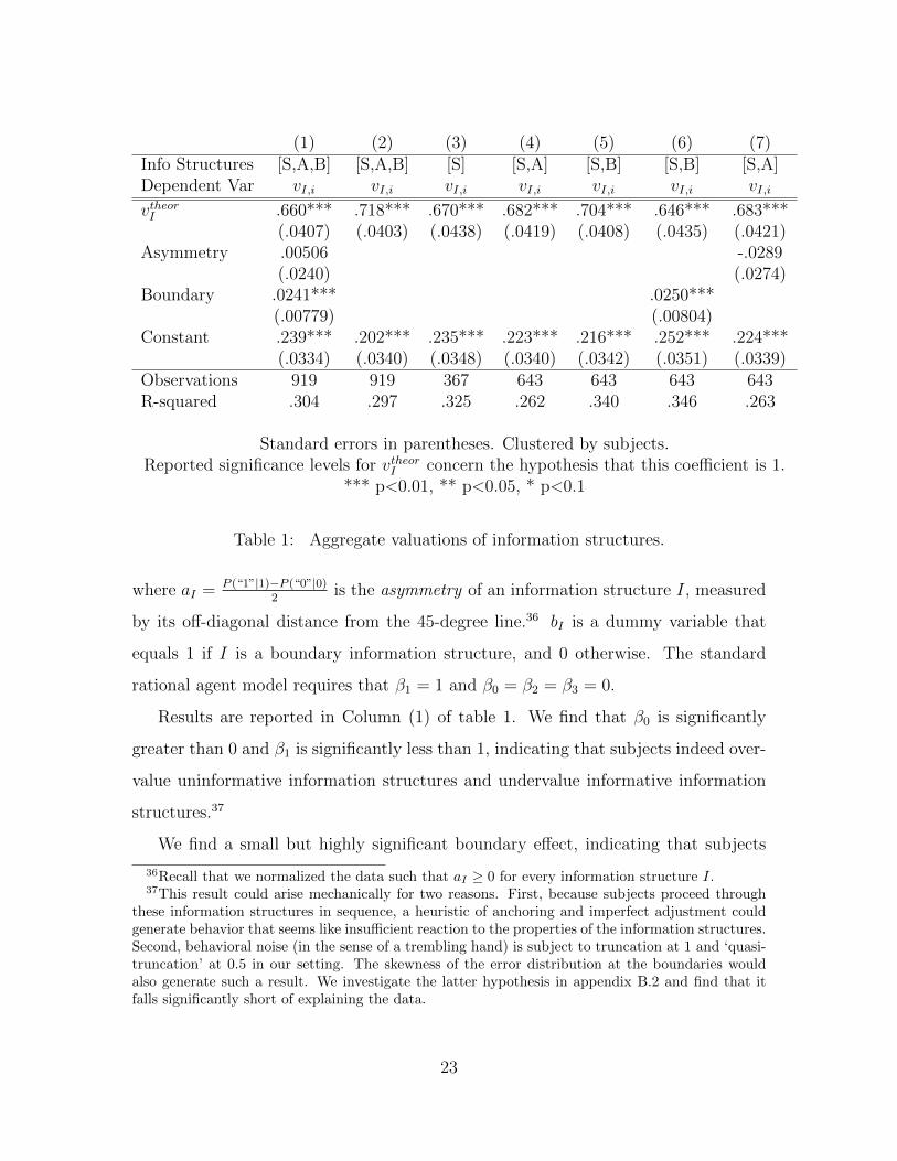
(1) (2) (3) (4) (5) (6) (7)Info Structures [S,A,B] [S,A,B] [S] [S,A] [S,B] [S,B] [S,A]Dependent Var vI,i vI,i vI,i vI,i vI,i vI,i vI,i

vtheorI .660*** .718*** .670*** .682*** .704*** .646*** .683***(.0407) (.0403) (.0438) (.0419) (.0408) (.0435) (.0421)

Asymmetry .00506 -.0289(.0240) (.0274)

Boundary .0241*** .0250***(.00779) (.00804)

Constant .239*** .202*** .235*** .223*** .216*** .252*** .224***(.0334) (.0340) (.0348) (.0340) (.0342) (.0351) (.0339)

Observations 919 919 367 643 643 643 643R-squared .304 .297 .325 .262 .340 .346 .263

Standard errors in parentheses. Clustered by subjects.Reported significance levels for vtheorI concern the hypothesis that this coefficient is 1.

*** p<0.01, ** p<0.05, * p<0.1

Table 1: Aggregate valuations of information structures.

where aI = P (“1”|1)−P (“0”|0)2

is the asymmetry of an information structure I, measured

by its off-diagonal distance from the 45-degree line.36 bI is a dummy variable that

equals 1 if I is a boundary information structure, and 0 otherwise. The standard

rational agent model requires that β1 = 1 and β0 = β2 = β3 = 0.

Results are reported in Column (1) of table 1. We find that β0 is significantly

greater than 0 and β1 is significantly less than 1, indicating that subjects indeed over-

value uninformative information structures and undervalue informative information

structures.37

We find a small but highly significant boundary effect, indicating that subjects

36Recall that we normalized the data such that aI ≥ 0 for every information structure I.37This result could arise mechanically for two reasons. First, because subjects proceed through

these information structures in sequence, a heuristic of anchoring and imperfect adjustment couldgenerate behavior that seems like insufficient reaction to the properties of the information structures.Second, behavioral noise (in the sense of a trembling hand) is subject to truncation at 1 and ‘quasi-truncation’ at 0.5 in our setting. The skewness of the error distribution at the boundaries wouldalso generate such a result. We investigate the latter hypothesis in appendix B.2 and find that itfalls significantly short of explaining the data.

23

have a preference for information structures where one signal realization removes all

uncertainty, on the order of 2.4 percentage points.38

We do not find asymmetry effects.

To be sure that our results are not driven by functional form mis-specification,

we check that they are not changed when assessing cleanly comparable subsets of

the data. The over-value/under-value phenomenon persists even when we no longer

include aI and bI in the regression (Column 2), when we consider only symmetric,

evenly spaced information structures (Column 3), when we exclude all boundary in-

formation structures (Column 4), and when we exclude all asymmetric non-boundary

information structures (Column 5).

Boundary effects persist, even when we only compare boundary information struc-

tures to symmetric information structures (Column 6), and their magnitude is not

substantially changed.

We do not find asymmetry effects, even when we compare only non-boundary

asymmetric information structures with symmetric information structures (Column

7). While in this case the sign of β2 is negative, it is not statistically significant.

To assess the magnitude of the estimated coefficient, note the information structure

(0.5, 1) has the maximum possible asymmetry, which is 0.25. This information struc-

ture is predicted to be valued only 0.7 percentage points less highly than the equally

informative, perfectly symmetric information structure (0.75, 0.75).

Result 1. In the Information Valuation Task,

(i) Subjects tend to overvalue less informative information structures and under-

value highly informative information structures.

(ii) We find highly significant positive boundary effects of approximately 2.4 percent-

age points.

38This result is virtually unchanged when we exclude all individuals who expressed a posteriortwo or more categories below 100% in the cases where the Bayesian posterior is 1.

24

(iii) We find no evidence of asymmetry effects.

4.1 Is the demand for information driven by belief updating?

If subjects have non-standard belief-updating procedures, that could cause non-

standard valuations of information structures. Alternatively, subjects could exhibit

non-standard information valuations because, even conditional on their own beliefs,

they have behavioral traits that affect how they value information. We use the data

elicited in the Belief Updating Task and the Signal Probability Assessment task to

distinguish these hypotheses. The resulting exercise also establishes that beliefs have

a causal effect on the demand for information in our experiment.

We define the empirically predicted valuation as

vpredI,i = PI,i(“1”)PI,i(1|“1”) + PI,i(“0”)PI,i(0|“0”) (4)

vpredI,i is the valuation for information structure I that would be elicited from a

subject with classical preferences over information, if she did not face an objective

lottery, but instead faced a subjective lottery with probabilities determined by her

reported beliefs.

Figure 4 is analogous to figure 3, but subjects’ valuations are now compared

to the empirical benchmark vpredI,i instead of the theoretical benchmark vtheorI . The

over-value/under-value phenomenon seems to disappear, as do the boundary effects.

Moreover, valuations appear to be too low, on average.

Are non-standard information valuations indeed caused by subjects’ beliefs? A

naıve empirical strategy would be to regress vI,i on vpredI,i , aI , and bI . The results

from this are reported in Column (1) of Table 2. This strategy is problematic for two

reasons. First, beliefs may be measured with error. If so, attenuation bias would lower

the estimated coefficient on vpredI,i . Second, there may be reverse causation: Having

25

-.12

-.09

-.06

-.03

0.0

3.0

6.0

9Va

luat

ion

- val

uatio

n pr

edic

ted

usin

g em

piric

al p

oste

riors

S1 S2 A1 A2 S3 B1 A3 B2 S4 B3Information Structure

S1

S2

A1

A2

S3

B1

A3

B2

S4

B3

.5.6

.7.8

.91

P("1

"|1)

.5 .6 .7 .8 .9 1P("0"|0)

Information Structures

Figure 4: Mean deviation of valuation vI,i from the empirical benchmark vpredI,i .Information structures are arranged in order of increasing informativeness. Standarderrors clustered by subject.

reported their valuations, subjects may be primed to report self-consistent ex post

beliefs.39 This would raise the estimated coefficient on vpredI,i .

Consequently, we instrument for vpredI,i with the Bayesian valuation, vtheorI,i . The

identifying assumption is that the correct Bayesian beliefs affect subjects’ valuations

only via their subjective beliefs.40 We report first-stage regressions of vpredI,i on vtheorI,i

in Column (2) of Table 2. This confirms that the instrument is relevant, since it

covaries with vpredI,i .

We report the results of IV estimation in Columns (3) of Table 2. The coefficient

on vpredI,i is strongly positive, and not significantly different from 1 (p = .229). This

suggests that subjects’ non-standard belief updating procedures have a causal impact

on their willingness to pay for information. The boundary dummy is slightly, but

significantly, negative. This indicates that the positive boundary effects in the pre-

39Reverse causation seems unlikely: Each subject is asked to evaluate ten different informationstructures, and, for each information structure, there are nine intervening choice problems betweenthe elicitation of values and the elicitation of ex post beliefs. Reporting self-consistent beliefs wouldthus be an impressive feat of memory.

40This exclusion restruction would not hold if, for instance, subjects were subconsciously influencedby the correct Bayesian posteriors when evaluating information structures, but this influence wasnot reflected in their ex post beliefs.

26

(1) (2) (3)Method OLS OLS IV

Dependent Var vI,i vpredI,i vI,i

vpredI,i .662*** 1.086(.0741) (.0712)

vtheorI,i .608***(.0266)

Asymmetry -.0251 -.020 .0272(.0275) (.0162) (.0275)

Boundary .0189 .060*** -.0415***(.0139) (.0053) (.0117)

Constant .234*** .309*** -.0962*(.0600) (.0221) (.0561)

Instrument vtheorI,i

Observations 919 919 919R-squared .342 .501 .252

Standard errors in parentheses. Clustered by subjects.

Reported significance levels for vpredI concernthe hypothesis that this coefficient is 1.

*** p<0.01, ** p<0.05, * p<0.1

Table 2: Relationship between beliefs and valuations.

vious section operate mainly through the subjects’ belief-updating procedures. The

negative constant term in Column (3) indicates that subjects undervalue informa-

tion, even conditional on their own subjective beliefs, by about 9.6 percentage points

(p = .086).

In Result 1, we identified two non-standard features of information demand; sub-

jects overvalue less informative information structures and undervalue highly infor-

mative information structures, and exhibit positive boundary effects. The analysis

above indicates, however, that subjects’ information demand exhibits a one-to-one

response to their own subjective beliefs, and does not exhibit positive boundary ef-

fects once subjective beliefs are controlled for. We conclude that both behavioral

anomalies identified in Result 1 operate through the channel of non-standard belief

27

updating.41

Result 2. Non-standard information demand is substantially explained by non-standard

belief updating. Subjects under-value information even relative to their own beliefs.

5 Consistent Individual Heterogeneity

It is clear from the preceding section that belief-updating is a multi-faceted phe-

nomenon. Subjects deviate from the standard model in several ways: They over-

respond to low-information signals and under-respond to high-information signals.

They also exhibit certainty effects. In this section, we investigate individual-level

variation in information demand and belief-updating. Even though belief-updating

is a complex phenomenon, we find that a one-parameter model captures much of the

variation in behavior across subjects.

First, we demonstrate that individual deviations from the mean valuations are not

i.i.d. but are consistent within subjects: a subject who overvalues some information

structures tends to overvalue all information structures, and by a similar amount. An

analogous statement holds for belief updating.

We then show that individual belief updating behavior predicts individual infor-

mation demand.42 Using only data from the Belief Updating Task, we estimate a

single-parameter model of responsiveness to information. Estimating a value of this

parameter for each subject, we generate out-of-sample estimates of behavior in the

Information Valuation Task. This simple model explains more than 80% of that part

41Moreover, we do not find asymmetry effects even controlling for subjects’ belief-updating. Henceit is not the case that the absence of asymmetry effects relative to the Bayesian benchmark is causedby a preference for symmetric information structures and a counterveiling belief-updating bias.

42One might worry that such a correlations could be spuriously caused by factors such as subjects’differential tendencies to avoid extreme options in the multiple price lists, or by framing effectsthat differentially affect individuals. Such factors, however, could not explain the out-of-samplepredictive power of responsiveness to information in the Gradual Information Task analyzed insection 5.4. Moreover, appendix B.3 shows that subjects’ responsiveness to information is stablewithin and across the Belief Updating and Information Valuation Tasks even when these factors arestatistically controlled for.

28

of non-standard valuation behavior that is due to non-standard belief updating.

Finally, we show that responsiveness to information is significantly correlated with

behavior in a second out-of-sample environment, the Gradual Information Task.

From this we conclude that responsiveness to information is a personality trait

that is stable across different choice environments. It is orthogonal to measures of

mathematical aptitude and cognitive style, including subjects’ self-reported knowl-

edge of Bayes’ law.

5.1 Are individuals consistent within tasks?

We find evidence that subjects have internally consistent directional biases, both in

information valuation and in belief updating.

Formally, we define the difference between subject i’s valuation of information

structure I and the theoretical benchmark by ∆vI,i := vI,i − vtheorI,i . Similarly, we

define the difference between subject i’s posterior and the theoretical benchmark by

∆PI,i(σ|“σ”) = logit(PI,i(σ|“σ”))− logit(PI(σ|“σ”)), where logit(x) = log(

x1−x

).

Recall that, for each task, we have 10 observations per subject, one for each infor-

mation structure. If subjects are internally consistent within a task, then if we split

our sample, a subject’s average deviation for two of the information structures should

be highly correlated with her average deviation for the other eight. We calculate

these correlations for each task, taking the average over all possible sample splits into

subsets of 2 and 8 information structures.43 These correlations are 0.765 (s.e. 0.041)

in the case of ∆vI,i, 0.707 (s.e. 0.51) in the case of ∆PI,i(1|“1”), and 0.580 (0.075)

in the case of ∆PI,i(0|“0”).44 All of them are highly significantly positive. This is

robust to alternative methods of measuring consistency, such as the Cronbach alpha

statistic.45

43We control for order and session fixed effects.44To perform this exercise with ∆PI,i(0|“0”) we drop the boundary information structures, and

split the sample in pieces of two and five information structures. This is because logit(x) is undefinedfor x = 1. We bootstrap the standard errors by drawing 1000 bootstrap samples.

45For a vector (X1, . . . , Xn) of random variables, Cronbach’s alpha is defined by α(X1, . . . , Xn) =

29

We summarize this finding in the following result:

Result 3. Subjects are internally consistent within tasks. Individual deviations from

the theoretical benchmark for valuations are highly correlated across information struc-

tures. The same holds for posterior beliefs.

5.2 A structural model of responsiveness to information.

Why do our subjects exhibit this consistency? We hypothesize that subjects dif-

fer in their responsiveness to information, a personal characteristic that scales the

movement of their beliefs upon receiving information.

We estimate a structural model of individual responsiveness to information as

follows: Note that for a Bayesian with prior p = P (s = 1) and information structure

I the following formula defines the posterior q(“σ”) = PI(s = 1|“σ”):

logit(q(“σ”)︸ ︷︷ ︸posterior

) = logit( p︸︷︷︸prior

) + log

(PI(“σ”|1)

PI(“σ”|0)

)︸ ︷︷ ︸

log-likelihood ratio

(5)

where logit(x) := log(

x1−x

). Hence, a Bayesian attaches weight 1 to the log-likelihood

ratio of the data. We generalize (5) to let each subject i be more or less responsive

to information than a Bayesian, by allowing for weight αi on the log-likelihood ratio

nn−1

[1−

∑i var(Xi)

var(∑

iXi)

]. Higher values signify higher internal consistency. The Cronbach alpha statistic

is 0.899, 0.875 and 0.737 for ∆vI,i, ∆PI,i(1|“1”), and ∆PI,i(0|“0”), respectively. With the exceptionof ∆PI,i(0|“0”), this compares favorably with the standard benchmark of 0.8, indicating a highconsistency of behavior within parts of the experiment. See e.g., Kline (1999).

30

of the data.46

logit(qi(“σ”)) = logit(pi) + αi log

(PI(“σ”|1)

PI(“σ”|0)

)(6)

The parameter αi is subject i’s responsiveness to information. Using only the data

from the Belief Updating Task, we estimate separately for each subject the following

seemingly unrelated regressions (SUR) model:47

logit(PI,i(1|“1”))

logit(PI,i(0|“0”))

= αi

log(PI(“1”|1)PI(“1”|0)

)log(PI(“0”|0)PI(“0”|1)

)+

ε1I,i

ε0I,i

(7)

Logit priors do not enter this equation because p = 1/2 in the Belief Updating

Task, and hence logit(pi) = 0.48

We do not assert that this one-parameter model fully captures belief-updating

behavior. In particular, it does not produce the over-value/under-value phenomenon

or the certainty effects that we have documented in Section 4. This is a deliberately

minimal model, selected to be transparent and to avoid over-fitting.49

Figure 5 displays the range of the estimated parameters αi. Our average subject

is Bayesian – the mean αi is 1.029. The αi are quite variable across subjects, with

46Grether (1980) and Holt and Smith (2009) estimate a similar models. Grether’s specificationdiffers from ours in that he also allows the weight (denoted β) on the logit prior to differ from 1. Weconsider this unattractive: for any β > 1, observing a sequence of signals from a perfectly uninfor-mative information structure lets beliefs converge to 1 or 0, whereas for any β < 1, observing sucha sequence lets beliefs converge to 0.5, regardless of the prior. Holt and Smith’s specification differsfrom ours in that they include a constant term in their regression. We consider this unattractive fora similar reason: for any constant term that differs from zero, observing a sequence of signals froma perfectly uninformative information structure lets beliefs converge to 1 or 0.

47We use the seemingly unrelated regression procedure rather than ordinary least squares, becauseit seems plausible that the errors ε1I,i and ε0I,i on PI,i(1|“1”) and PI,i(0|“0”) are correlated for anygiven information structure, and hence the SUR procedure provides us with more efficient estimates.We use the data on all the information structures but the boundary information structures f , h,and j to estimate (7). We do so because the logit(PI,i(0|“0”)) is not defined when PI,i(0|“0”) = 1,which is frequently the case for boundary information structures.

48Section 5.4 shows that our estimates of responsiveness to information have predictive power evenin the Gradual Information Task, in which subjects update from non-uniform priors in most cases.

49Enrico Fermi attributed the following quote to John von Neumann: “With four parameters Ican fit an elephant, and with five I can make him wiggle his trunk.” (Dyson (2004))

31

0.5

11.

52

Estim

ated

alp

ha

Subject

Figure 5: The estimated responsiveness parameters αi by subject. Subjects orderedby αi.

a standard deviation of 0.266, a minimum of 0.196 and a maximum of 2.191. We

reject the null hypothesis that αi = 1 at the 5% level for 37% (34 of 92) subjects. In

Appendix A we show that both the level of responsiveness, and the extent to which

responsiveness differs from the Bayesian value of 1 are unrelated to measures of math-

ematical aptitude and cognitive style, including subjects’ self-reported knowledge of

Bayes’ law.

5.3 Are individuals consistent across tasks?

If responsiveness to information is a stable individual trait, then our individual-level

estimates of responsiveness should explain behavior in the Information Valuation Task

(an out-of-sample environment). If responsiveness to information is an important trait

in our setting, then we should not gain much explanatory power by using the belief

updating data in a way that allows for idiosyncratic deviations for each information

structure rather than by using responsiveness alone.

Before we test these hypotheses, we establish that subject behavior is indeed

correlated across the Information Valuation Task and the Belief Updating Task. For

32

a given information structure, the partial correlation between ∆vI,i and ∆PI,i(0|“0”)+

∆PI,i(1|“1”), controlling for vtheorI,i , is .339 (p < .0001). Hence, a subject’s valuations

of each information structure are substantially explained by her posterior beliefs for

that information structure, even after we control for informativeness.

To investigate what part of the variation in information demand we can explain

using responsiveness to information we proceed more structurally. We use the data

from the Belief Updating Task to construct two distinct predictors of information

demand behavior, and compare their explanatory power.

Our unconstrained predictor ∆vpredI,i uses each subject’s posterior beliefs to predict

how far her valuation of an information structure should deviate from the Bayesian

benchmark separately for each information structure. This permits idiosyncratic de-

viations for each information structure. Hence, it may be influenced by many dis-

tinct belief updating biases along which individuals may be heterogenous, such as

different degrees of nonlinear probability weighting, different insensitivity to signal

characteristics, different rules of thumb, and so on. It also captures the over-value /

under-value effect and the boundary effects we documented in section 4. Formally,

our unconstrained predictor of individual i’s deviation for information structure I is

∆vpredI,i := vpredI,i − vtheorI .50

Our constrained predictor ∆vI(αi) uses only a subject’s estimated parameter of

responsiveness to predict how far her valuations should deviate from the Bayesian

benchmark. That is, for each subject and each information structure, we use that

subject’s αi to predict her posterior beliefs PI(σ|“σ”; αi) and valuations vI(αi) =

PI(“1”)PI(1|“1”; αi)+PI(“0”)PI(0|“0”; αi). We then define the constrained predictor

∆vI(αi) := vI(αi) − vtheorI . This predictor permits variation only via the estimated

parameter αi.

We compare the explanatory power of our predictors ∆vpredI,i and ∆vI(αi) by esti-

50Alternatively, one could exclude data from the Signal Probability Assessment task, and constructvupdI,i = P (“1”)PI,i(1|“1”) + P (“0”)PI,i(0|“0”). This specification uses the true signal probabilitiesand the elicited posterior beliefs. The results that follow are essentially unchanged if we use thisspecification instead.

33

mating the following model

∆vI,i = β0 + β1∆vpredI,i + β2∆vI(αi) + εi (8)

We interpret the R2-coefficient of this model as the maximal part of the variance

in the valuations of information structures that can be explained by belief updating.

To assess how well our model of responsiveness explains this variance, we estimate

model (8) with β1 restricted to 0.

The results are in Column 1 and 2 of table 3.51 The R2 of the unconstrained

model is 22.8%, which compares to an R2 of 19.4% for the constrained model.52 This

shows that a single subject-level parameter captures most (85.1%) of the variation in

valuations that can be explained by non-standard belief updating.53 Once we know

a subject’s general responsiveness to information, a subject’s specific ex post beliefs

contribute little explanatory power. Notably, the R2 in both column (1) and (2) are

more than double the R2 yielded by regressing ∆vI,i on all the demographic variables

from our post-experiment questionnaire (which is 8.8%). We refer interested readers

to Section 6 and Appendix A. For completeness, Column 3 reports the estimates of

model (8) when β2 is set to 0.54

∆vI(αi) performs well not just as a predictor, but as a prediction: The slope

parameter in Column 2 is not significantly different from 1, and the intercept term

is only slightly (but significantly) different from 0. ∆vI(αi) is a close-to-unbiased

prediction of behavior in the Information Valuation Task, with a systematic error of

51Since we use estimates of αi as explanatory variables, we bootstrap the standard errors. We usethe following semiparametric procedure: For each subject we first draw a responsiveness parameterαi according to the distribution of his estimate of this parameter. We then select a bootstrap sampleand perform the estimations. We draw a total of 1000 bootstrap samples.

52The difference between these R2 values is significant at all conventional levels. (Testing thatthe R2 coefficient of the model in column 1 is significantly larger than in the model in column 2is equivalent to testing that the coefficient on ∆vpredI,i is zero in the model in column 1, see Greene(2008), chapter 5.)

53We show in appendix B.4 that this is not driven by a particular set of information structures.54Notably, the R-squared in this instance is lower than that of the constrained model. This suggests

that the constrained model exploits underlying structure in the data - the stability of behavior acrosschoice problems in the same task - to produce better estimates.

34

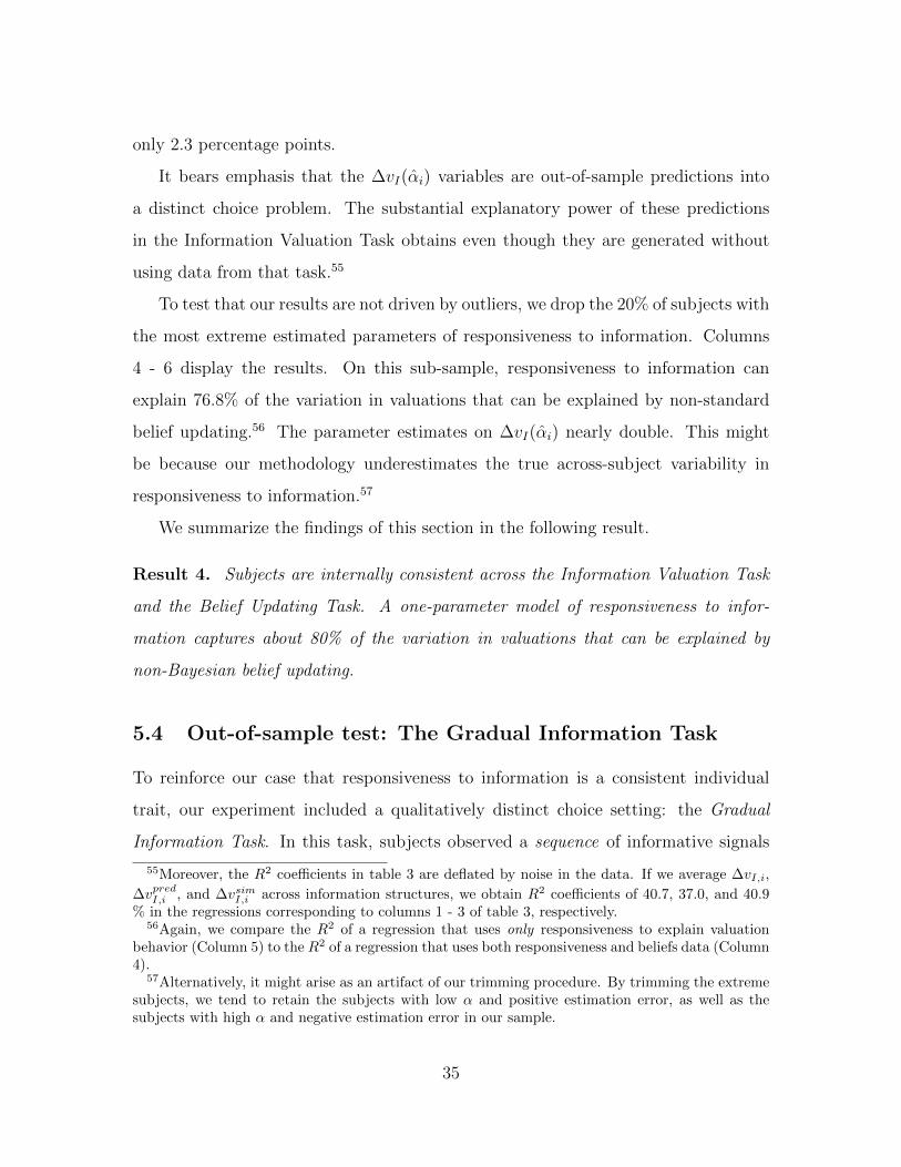
only 2.3 percentage points.

It bears emphasis that the ∆vI(αi) variables are out-of-sample predictions into

a distinct choice problem. The substantial explanatory power of these predictions

in the Information Valuation Task obtains even though they are generated without

using data from that task.55

To test that our results are not driven by outliers, we drop the 20% of subjects with

the most extreme estimated parameters of responsiveness to information. Columns

4 - 6 display the results. On this sub-sample, responsiveness to information can

explain 76.8% of the variation in valuations that can be explained by non-standard

belief updating.56 The parameter estimates on ∆vI(αi) nearly double. This might

be because our methodology underestimates the true across-subject variability in

responsiveness to information.57

We summarize the findings of this section in the following result.

Result 4. Subjects are internally consistent across the Information Valuation Task

and the Belief Updating Task. A one-parameter model of responsiveness to infor-

mation captures about 80% of the variation in valuations that can be explained by

non-Bayesian belief updating.

5.4 Out-of-sample test: The Gradual Information Task

To reinforce our case that responsiveness to information is a consistent individual

trait, our experiment included a qualitatively distinct choice setting: the Gradual

Information Task. In this task, subjects observed a sequence of informative signals

55Moreover, the R2 coefficients in table 3 are deflated by noise in the data. If we average ∆vI,i,

∆vpredI,i , and ∆vsimI,i across information structures, we obtain R2 coefficients of 40.7, 37.0, and 40.9% in the regressions corresponding to columns 1 - 3 of table 3, respectively.

56Again, we compare the R2 of a regression that uses only responsiveness to explain valuationbehavior (Column 5) to the R2 of a regression that uses both responsiveness and beliefs data (Column4).

57Alternatively, it might arise as an artifact of our trimming procedure. By trimming the extremesubjects, we tend to retain the subjects with low α and positive estimation error, as well as thesubjects with high α and negative estimation error in our sample.

35

(1) (2) (3) (4) (5) (6)VARIABLES ∆vI,i ∆vI,i ∆vI,i ∆vI,i ∆vI,i ∆vI,i

∆vpredI,i 0.296*** 0.530*** 0.309*** 0.448***(0.070) (0.094) (0.084) (0.104)

∆vI(αi) 0.814 1.123 1.678 2.053**(0.200) (0.204) (0.497) (0.532)

Constant -0.027*** -0.023*** -0.030*** -0.0282*** -0.0246*** -0.029***(0.007) (0.007) (0.007) (0.007) (0.008) (0.008)

Observations 919 919 919 729 729 729R-squared 0.228 0.194 0.157 0.190 0.146 0.10210 percent trim no no no yes yes yes

Bootstrapped standard errors in parentheses.*** p<0.01, ** p<0.05, * p<0.1

Significance levels on the slope parameters concern the hypothesis that the coefficients are 1.

Table 3: Explaining and decomposing deviations from benchmark valuations.

about the state of the world, and made choices that revealed when their certainty

about the underlying state crossed a given threshold.

Specifically, the Gradual Information Task was played in four blocks. In each

block, subjects were shown a pair of boxes, each containing some combination of 20

balls (black or white). At the start of each block, the computer randomly selected a

box, each with 50% probability, and showed the subject a sequence of 12 draws with

replacement from the Selected Box.58 After each draw, subjects indicated whether

they would rather (i) receive $35 if Box X was the Selected Box (ii) receive $35 if Box

Y was the Selected Box, or (iii) receive $35 with probability q for some fixed success

probability q. No choice would prematurely end the sequence of draws, or preclude

any future choices.

Subjects were in effect being asked, given the draws they had seen so far, whether

they were at least 100 × q% sure which box had been selected.59 Subjects faced,

58Each subject’s balls were drawn independently of other subjects’ balls.59In this part, all subjects went through the information structures in the same order.

36

in this order, the symmetric information structures (0.7, 0.7), (0.8, 0.8), (0.7, 0.7) and

(0.6, 0.6), with q equal to 0.8, 0.9, 0.8 and 0.75 respectively.60

This task differs from the Information Valuation Task and the Belief Updating

Task in several ways.

(i) The Belief Updating Task asks subjects to report how certain they are for a

given amount of information. The Gradual Information Task asks subjects to

report how much information they need to attain a given level of certainty.

(ii) The previous tasks require the subject only consider one signal at a time,

whereas the Gradual Information Task requires the subject to make aggregative

assessments from a long sequence of signals.

(iii) In the previous tasks, subjects update a symmetric prior for each information

structure, whereas in the Gradual Information Task subjects have asymmetric

priors after the first signal.61

(iv) The Belief Updating Task uses the strategy method to elicit choices (a cold

state measure), while the Gradual Information Task displays signal draws to

subjects and asks them for a decision after the fact (a hot state measure).

(v) In the Gradual Information Task subjects make ternary decisions whereas in

the previous tasks they (essentially) reported a continuous variable.

Our strategy is to take the estimates of each individual’s responsiveness from the

Belief Updating Task, and generate predictions of that individual’s behavior in the

Gradual Information Task. We use these to assess the stability of responsiveness

across different choice environments.

How would an agent perfectly described by the responsiveness model (equation

(6)) behave in the Gradual Information Task? Let dt be a variable equal to 1 if a

60This implies that a Bayesian decides to bet on a box as soon as he has seen two more balls ofone rather than the other color in blocks 1 to 3, and 3 more balls in block 4.

61Arithmetically, having a symmetric prior simplifies Bayesian updating substantially.

37

!!!!!!!

qI#

logit(#ptI,i#)#

t#

Bayesian#belief#stream#!

simulated#belief#stream#(αi#<#1)#

!

∆bI,i#

Figure 6: Random walk of beliefs under the Responsiveness model

black ball is drawn in period t, and -1 otherwise. Her posterior belief that the selected

box is box X, ptI,i, is described by:

logit(ptI,i) = logit(pt−1I,i ) + αidt log

(PI(“1”|1)

PI(“1”|0)

)(9)

Thus, conditional on the box selected, her logit-beliefs follow a random walk with

drift, where the responsiveness parameter αi scales the rate of movement. When she

faces an outside option that yields a prize with probability qI , she first bets on a box

when max{ptI,i, 1 − ptI,i} ≥ qI . Hence, we expect individuals who are less responsive

to information to require more information before they are willing to bet on a box.

Figure 6 illustrates.

We measure behavior in the Gradual Information Task as follows: We ask how

much more (or less) sure than qI a Bayesian would be, when subject i first bets on

a box. Suppose i first bets on a box at draw T when facing information structure

I. Then we take note of the difference between the Bayesian posterior bTI,i for that

38

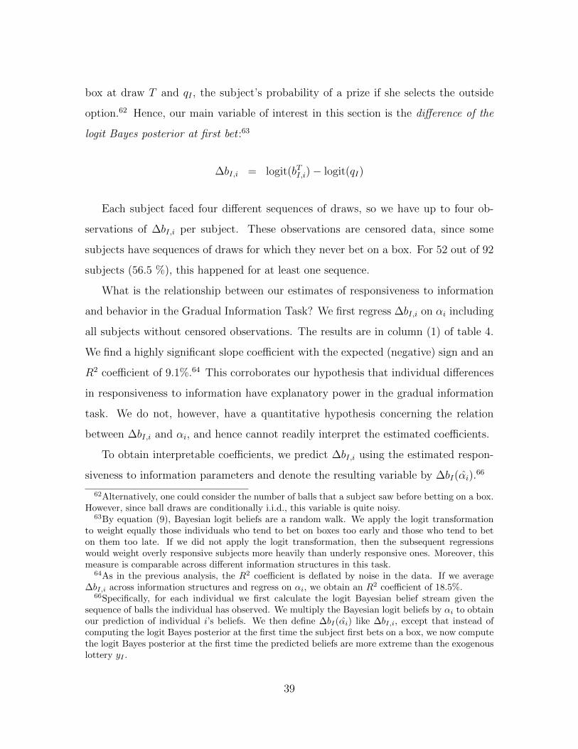
box at draw T and qI , the subject’s probability of a prize if she selects the outside

option.62 Hence, our main variable of interest in this section is the difference of the

logit Bayes posterior at first bet :63

∆bI,i = logit(bTI,i)− logit(qI)

Each subject faced four different sequences of draws, so we have up to four ob-

servations of ∆bI,i per subject. These observations are censored data, since some

subjects have sequences of draws for which they never bet on a box. For 52 out of 92

subjects (56.5 %), this happened for at least one sequence.

What is the relationship between our estimates of responsiveness to information

and behavior in the Gradual Information Task? We first regress ∆bI,i on αi including

all subjects without censored observations. The results are in column (1) of table 4.

We find a highly significant slope coefficient with the expected (negative) sign and an

R2 coefficient of 9.1%.64 This corroborates our hypothesis that individual differences

in responsiveness to information have explanatory power in the gradual information

task. We do not, however, have a quantitative hypothesis concerning the relation

between ∆bI,i and αi, and hence cannot readily interpret the estimated coefficients.

To obtain interpretable coefficients, we predict ∆bI,i using the estimated respon-

siveness to information parameters and denote the resulting variable by ∆bI(αi).66

62Alternatively, one could consider the number of balls that a subject saw before betting on a box.However, since ball draws are conditionally i.i.d., this variable is quite noisy.

63By equation (9), Bayesian logit beliefs are a random walk. We apply the logit transformationto weight equally those individuals who tend to bet on boxes too early and those who tend to beton them too late. If we did not apply the logit transformation, then the subsequent regressionswould weight overly responsive subjects more heavily than underly responsive ones. Moreover, thismeasure is comparable across different information structures in this task.

64As in the previous analysis, the R2 coefficient is deflated by noise in the data. If we average∆bI,i across information structures and regress on αi, we obtain an R2 coefficient of 18.5%.

66Specifically, for each individual we first calculate the logit Bayesian belief stream given thesequence of balls the individual has observed. We multiply the Bayesian logit beliefs by αi to obtainour prediction of individual i’s beliefs. We then define ∆bI(αi) like ∆bI,i, except that instead ofcomputing the logit Bayes posterior at the first time the subject first bets on a box, we now computethe logit Bayes posterior at the first time the predicted beliefs are more extreme than the exogenouslottery yI .

39

(1) (2) (3)VARIABLES ∆bI,i ∆bI,i ∆bI,i

αi -1.46**(0.600)

∆bI(αi) 1.067*** 6.088***(0.460) (1.731)

Constant 1.513** 1.930*** 0.662(0.631) (0.436) (0.651)

Method OLS Tobit TobitObservations 152 368 29210-percent trim no no yesR2 / pseudo-R2 0.091 0.065 0.076

Bootstrapped standard errors in parentheses.65

*** p<0.01, ** p<0.05, * p<0.1

Table 4: Predicting behavior in the gradual information task. Model (1) excludesall subjects with a censored observation. Model (2) includes all subjects and obser-vations. Model (3) excludes the subjects with parameters αi more extreme than the10th or 90th percentile.

We then regress ∆bI,i on ∆bI(αi). To account for censoring, we estimate a Tobit

censored regression model. The censoring level for subject i and information structure

I is the most extreme difference between the logit Bayes posterior and logit(qI) that

individual i has faced in block I. We estimate this model using maximum likelihood.

We continue to assess goodness-of-fit as the fraction of variance in the dependent

variable that is explained by the dependent variable. The pseudo-R2 measure by

McKelvey and Zavoina (1975) has this interpretation.67

Columns (2) and (3) in Table 4 report the results. Column (2) uses all subjects,

whereas column (3) drops the 20% of subjects with the most extreme αi.

The positive constants in columns (2) and (3) corroborate previous findings (Pe-

terson and Beach (1967)) that subjects update more conservatively when aggregating

sequences of signals than when making single-signal inferences.

On both samples our estimates of responsiveness to information are highly signif-

67In our context, the McKelvey and Zavoina (1975) R2 is defined by R2MZ =

var(∆bI,i)var(∆bI,i)+var(ε) .

40

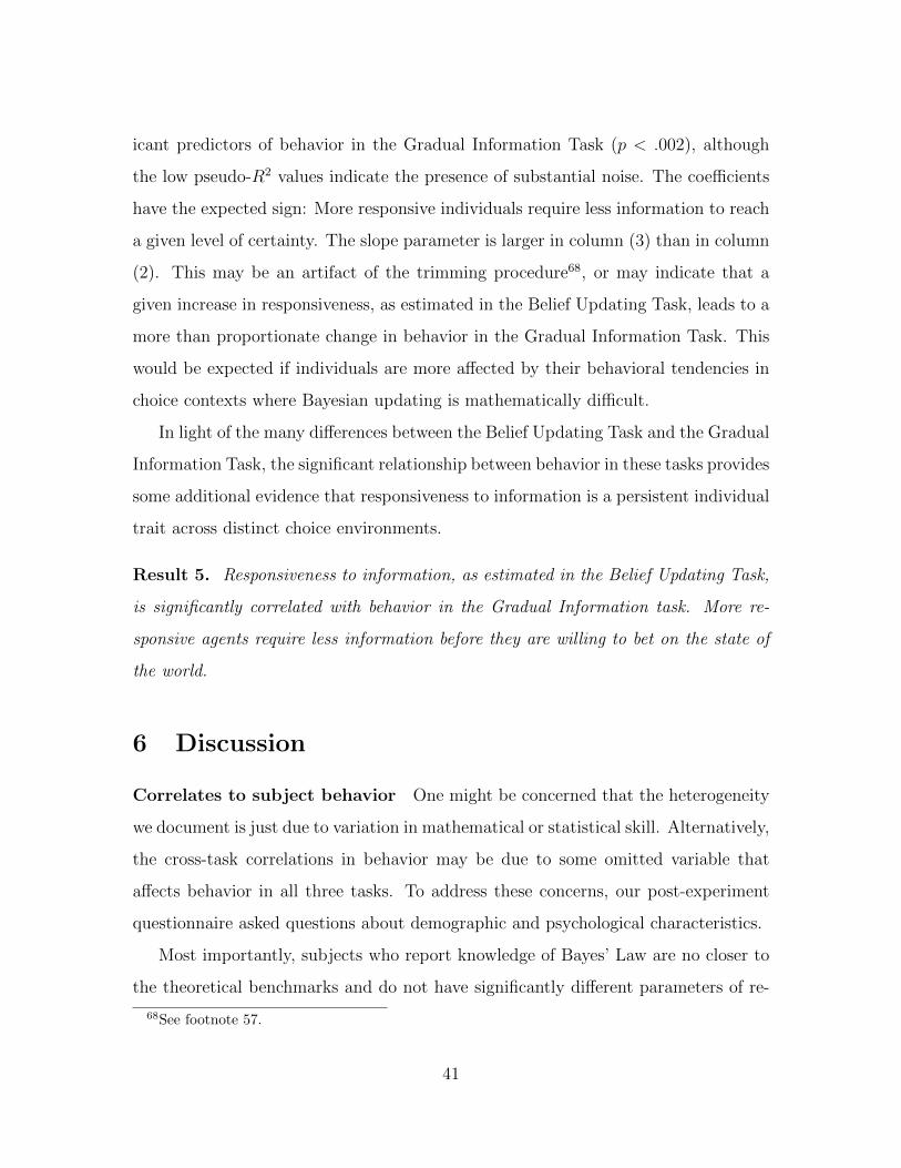
icant predictors of behavior in the Gradual Information Task (p < .002), although

the low pseudo-R2 values indicate the presence of substantial noise. The coefficients

have the expected sign: More responsive individuals require less information to reach

a given level of certainty. The slope parameter is larger in column (3) than in column

(2). This may be an artifact of the trimming procedure68, or may indicate that a

given increase in responsiveness, as estimated in the Belief Updating Task, leads to a

more than proportionate change in behavior in the Gradual Information Task. This

would be expected if individuals are more affected by their behavioral tendencies in

choice contexts where Bayesian updating is mathematically difficult.

In light of the many differences between the Belief Updating Task and the Gradual

Information Task, the significant relationship between behavior in these tasks provides

some additional evidence that responsiveness to information is a persistent individual

trait across distinct choice environments.

Result 5. Responsiveness to information, as estimated in the Belief Updating Task,

is significantly correlated with behavior in the Gradual Information task. More re-

sponsive agents require less information before they are willing to bet on the state of

the world.

6 Discussion

Correlates to subject behavior One might be concerned that the heterogeneity

we document is just due to variation in mathematical or statistical skill. Alternatively,

the cross-task correlations in behavior may be due to some omitted variable that

affects behavior in all three tasks. To address these concerns, our post-experiment

questionnaire asked questions about demographic and psychological characteristics.

Most importantly, subjects who report knowledge of Bayes’ Law are no closer to

the theoretical benchmarks and do not have significantly different parameters of re-

68See footnote 57.

41

sponsiveness to information. Subjects’ choice of college major and performance in the

Cognitive Reflection Test are equally unable to explain responsiveness to information

or deviations from the theoretical benchmarks. This suggests that the inter-subject

variation in our experiment identifies behavioral traits, and is not simply due to

variations in calculative ability.

We find no significant demographic or psychological correlates of responsiveness to

information. We also test how well demographic and psychological variables explain

behavior in the Information Valuation Task. Regressing ∆vI,i on all psychological and

demographic variables we elicited yields an R2 coefficient of 8.8%. Including ∆vI,i(αi)

substantially and significantly increases R2 to 25.16%. Hence, responsiveness to in-

formation has explanatory power above and beyond demographic and psychological

characteristics.

A detailed analysis is presented in Appendix A.

Responsiveness to information and quantity of information demanded We

have investigated subjects’ willingness to pay for a single signal, and related this to

responsiveness. We have not investigated how many signals subjects would pay to see,

if each observation came at a price. We omitted this because the comparative statics

concerning responsiveness and quantity demanded are ambiguous. On one hand, for

a given prior, more responsive agents have a higher marginal value of information. On

the other hand, more responsive agents’ beliefs are quicker to attain extreme beliefs,

and agents with extreme beliefs have a lower marginal value of information. Hence,

the effect of a change in responsiveness on the quantity of information demanded

could be positive or negative.

Comparison to heterogeneous risk aversion Heterogeneous responsiveness to

information is not observationally equivalent to heterogeneous risk aversion. Our

experiment is one proof of this, since our results cannot be explained by classical risk

aversion.

42

To take a more natural example, heterogeneous responsiveness yields different

comparative statics for information purchasing. Consider an agent choosing between

a safe option and a risky option, who could purchase information that might affect

the optimal decision. If, in the absence of information, the agent would choose the

risky option, then his willingness to pay for information is increasing in risk aversion.

If, in the absence of information, the agent would choose the safe option, then his

willingness to pay for information is decreasing in risk aversion. By contrast, in both

cases, his willingness to pay for information is increasing in responsiveness. Appendix

C formalizes this argument.

7 Concluding Remarks

Economists study many situations where agents learn about their environment by

acquiring costly stochastic information. It is therefore important to understand in-

formation demand behavior, and its relationship to belief updating. In this article, we

examine information demand behavior and belief updating across a range of choice

contexts, using a novel experiment design.

In our experiment, we identify two biases of the population-level demand for

information. First, subjects over-value less informative information structures and

under-value more informative information structures. Second, they value boundary

information structures disproportionately highly.

These two biases do not persist when we condition on subjects’ elicited beliefs,

rather than the objective Bayesian posteriors. This suggests that these biases are the

result of non-standard belief updating procedures, rather than non-standard valua-

tions of information structures.

On the individual level, we find that subjects deviate from the theoretical pre-

dictions in internally consistent ways. We show that this consistency is explained by

responsiveness to information, an individual-specific parameter that connects behav-

43

ior across the parts in our experiment. A simple model of responsiveness explains

80% of the variation in information demand that is due to belief updating. The out-

of-sample predictions across different choice problems provide initial evidence that

responsiveness is a stable individual trait. Moreover, this trait provides substantial

explanatory power that is distinct from measures of mathematical aptitude and cog-

nitive style. Economic models may be improved by considering this new dimension

of heterogeneity.

The present study has investigated belief updating and the valuation of infor-

mation in choice problems where subjects have an objective prior, receive signals

with known error probabilities, and do not care about their beliefs per se. A key

outstanding question is whether subjects behave differently when learning about per-

sonal characteristics such as intelligence, health, or beauty. Belief-dependent utility

may alter the relationship between responsiveness and information demand; for in-

stance, more responsive subjects may place a lower value on information because they

foresee more extreme ex post beliefs. Additionally, future research may profitably in-

vestigate whether individuals exhibit consistent responsiveness to information when

facing Knightian uncertainty, by presenting subjects with rich qualitative signals as

from news reports or word-of-mouth.69

69Augenblick and Rabin (2013) find data that is suggestive of this hypothesis.

44

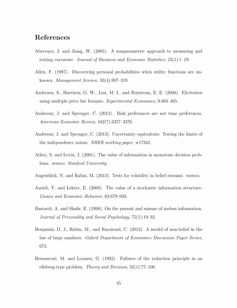
References

Abrevaya, J. and Jiang, W. (2005). A nonparametric approach to measuring and

testing curvature. Journal of Business and Economic Statistics, 23(1):1–19.

Allen, F. (1987). Discovering personal probabilities when utility functions are un-

known. Management Science, 33(4):307–319.

Andersen, S., Harrison, G. W., Lau, M. I., and Rutstrom, E. E. (2006). Elicitation

using multiple price list formats. Experimental Economics, 9:383–405.

Andreoni, J. and Sprenger, C. (2012). Risk preferences are not time preferences.

American Economic Review, 102(7):3357–3376.

Andreoni, J. and Sprenger, C. (2013). Uncertainty equivalents: Testing the limits of

the independence axiom. NBER working paper, w17342.

Athey, S. and Levin, J. (2001). The value of information in monotone decision prob-

lems. mimeo. Stanford University.

Augenblick, N. and Rabin, M. (2013). Tests for volatility in belief streams. mimeo.

Azrieli, Y. and Lehrer, E. (2008). The value of a stochastic information structure.

Games and Economic Behavior, 63:679–693.

Bastardi, A. and Shafir, E. (1998). On the pursuit and misuse of useless information.

Journal of Personality and Social Psychology, 75(1):19–32.

Benjamin, D. J., Rabin, M., and Raymond, C. (2013). A model of non-belief in the

law of large numbers. Oxford Department of Economics Discussion Paper Series,

672.

Bernasconi, M. and Loomes, G. (1992). Failures of the reduction principle in an

ellsberg-type problem. Theory and Decision, 32(1):77–100.

45

Burks, S. V., Carpenter, J. P., Goette, L., and Rustichini, A. (2013). Overconfidence

and social signaling. Review of Economic Studies, forthcoming.

Cabrales, A., Gossner, O., and Serrano, R. (2013a). The appeal of information trans-

actions. Working paper.

Cabrales, A., Gossner, O., and Serrano, R. (2013b). Entropy and the value of infor-

mation for investors. American Economic Review, 103(1):360–377.

Camerer, C. (1995). Individual decision making. In Kagel, J. H. and Roth, A. E.,

editors, Handbook of Experimental Economics, chapter 8, pages 587–683. Princeton

University Press.

Costa-Gomes, M. A., Huck, S., and Weizsaecker, G. (2012). Beliefs and actions

in the trust game: Creating instrumental variables to estimate the causal effect.

Discussion Paper, Wissenschaftszentrum Berlin fuer Sozialforschung, SP II 2012-

302.

Dyson, F. (2004). A meeting with Enrico Fermi. Nature, 427:297.

Eil, D. and Rao, J. M. (2011). The good news-bad news effect: Asymmetric processing

of objective information about yourself. American Economic Journal: Microeco-

nomics, 3:114–138.

Eliaz, K. and Schotter, A. (2010). Paying for confidence: An experimental study

of the demand for non-instrumental information. Games and Economic Behavior,

70:304–324.

Ergin, H. and Gul, F. (2009). A theory of subjective compound lotteries. Journal of

Economic Theory, 144:899–929.

Ertac, S. (2011). Does self-relevance affect information processing? experimental

evidence on the response to performance and non-performance feedback. Journal

of Economic Behavior and Organization, 80:532–545.

46

Fiedler, K. and Juslin, P., editors (2006). Information Sampling and Adaptive Cog-

nition. Cambridge University Press.

Fischbacher, U. (2007). z-tree: Zurich toolbox for ready-made economic experiments.

Experimental Economics, 10(2):171–178.

Frederick, S. (2005a). Cognitive reflection and decision making. Journal of Economic

perspectives, pages 25–42.

Frederick, S. (2005b). Cognitive reflection and decision making. The Journal of

Economic Perspectives, 19(4):25–42.

Gneezy, U., List, J. A., and Wu, G. (2006). The uncertainty effect: When a risky

prospect is valued less than it’s worst possible outcome. The Quarterly Journal of

Economics, 121(4):1283–1309.

Greene, W. H. (2008). Econometric Analysis. Pearson Prentice Hall, 6 edition.

Grether, D. M. (1980). Bayes rule as a descriptive model: The representativeness

heuristic. The Quarterly Journal of Economics, 95(3):537–557.

Grether, D. M. (1992). Testing bayes rule and the representativeness heuristic: Some

experimental evidence. Journal of Economic Behavior and Organization, 17(1):31–

57.

Halevy, Y. (2007). Ellsberg revisited: an experimental study. Econometrica,

75(2):503–536.

Halevy, Y. and Feltkamp, V. (2005). A bayesian approach to uncertainty aversion.

Review of Economic Studies, 72:449–466.

Hoelzl, E. and Rustichini, A. (2005). Overconfident: Do you put your money on it?

Economic Journal, 115(04):305–318.

47

Hoffman, M. (2012). How is information (under-) valued? evidence from framed field

experiments. mimeo.

Holt, C. A. and Laury, S. K. (2002). Risk aversion and incentive effects. American

Economic Review, 92(5):1644 – 1655.

Holt, C. A. and Smith, A. M. (2009). An update on bayesian updating. Journal of

Economic Behavior and Organization, 69:125–134.

Kahneman, D. and Tversky, A. (1972). Subjective probability: A judgement of

representativeness. Cognitive Psychology, 3:430–454.

Kahneman, D. and Tversky, A. (1974). Judgment under uncertainty: Heuristics and

biases. Science, 185(4157):1124–1131.

Karni, E. (2009). A mechanism for eliciting probabilities. Econometrica, 77(2):603–

606.

Keren, G. and Willemsen, M. C. (2008). Decision anomalies, experimenter as- sump-

tions and participants’ comprehension: Revaluating the uncertainty eect. Journal

of Behavioral Decision Making, 22(3).

Kline, P. (1999). Handbook of Psychological Testing. Routledge, London and New

York, 2 edition.

Kocher, M., Krawczyk, M., and van Winden, F. (2009). Let me dream on! anticipa-

tory emotions and preference for timing in lotteries. Working paper.

Koszegi, B. and Rabin, M. (2009). Reference-dependent consumption plans. American

Economic Review, 99(3):909–936.

Massey, C. and Wu, G. (2005). Detecting regime shifts: The causes of under- and

overreaction. Management Science, 51(6):932–947.

48

McKelvey, R. D. and Zavoina, W. (1975). A statistical model for the analysis of

ordinal level dependent variables. The Journal of Mathematical Sociology, 4(1):103–

120.

Milgrom, P. and Stokey, N. (1982). Information, trade and common knowledge.

Journal of Economic Theory, 26(1):17–27.

Moebius, M. M., Niederle, M., Niehaus, P., and Rosenblat, T. S. (2013). Managing

self-confidence: Theory and experimental evidence. mimeo.

Peterson, C. R. and Beach, L. R. (1967). Man as an intuitive statistician. Psychological

Bulletin, 68(1):29–46.

Peterson, C. R., Schneider, R. J., and Miller, A. J. (1965). Sample size and the revision

of subjective probabilities. Journal of Experimental Psychology, 69(5):522–527.

Roth, A. E. and Malouf, M. W. (1979). Game-theoretic models and the role of

information in bargaining. Psychological review, 86(6):574.

Rydval, O., Ortmann, A., Prokosheva, S., and Hertwig, R. (2009). How certain is the

uncertainty effect. Experimental Economics, 12:473–487.

Savage, L. J. (1954). Foundations of Statistics. Wiley, New York.

Scheier, M., Carver, C., and Bridges, M. (1994). Distinguishing optimism from neu-

roticism (and trait anxiety, self-mastery, and self-esteem): A re-evaluation of the

life orientation test. Journal of Personality and Social Psychology, 67:1063–1078.

Schlag, K. and van der Weele, J. (October 2009). Eliciting probabilities, means,

medians, variances and covariances without assuming risk neutrality. Technical

Report, Universitat Pompeu Fabra.

Seo, K. (2009). Ambiguity and second order belief. Econometrica, 77(5):1575 – 1605.

49

Shiller, R. J. (1981). Do stock prices move too much to be justified by subsequent

changes in dividends? American Economic Review, 71(3):421–436.

Simonsohn, U. (2009). Direct risk aversion: Evidence from risky prospects valued

below their worst outcome. Psychological Science, 20(6):686–692.

Tobacyk, J. and Milford, G. (1983). Belief in paranormal phenomena: Assessment

instrument development and implications for personality functioning. Journal of

Personality and Social Psychology, 44(5):1029–1037.

Yates, F. and Zukowski, L. (1976). Characterization of ambiguity in decision making.

Behavioral Science, 21:19–25.

Zimmermann, F. (2014). Clumped or piecewise? - evidence on preferences for infor-

mation. Management Science (forthcoming).

50

A Correlates of Responsiveness to Information

The last stage of our experiment was a questionnaire to elicit a range of demographic

and psychological measures from our subjects. We are interested in three questions:

(i) is responsiveness to information, and the deviation from the Bayesian benchmark,

explained by subjects’ self-reported knowledge of Bayes law, (ii) is responsiveness to

information correlated with demographic or psychological measures, and (iii) for the

behaviors that we explained in sections 5.2 and 5.4 using responsiveness to informa-

tion, how much explanatory power do we obtain by instead using demographic and

psychological variables?70

In our questionnaire, subjects first completed the Cognitive Reflection Test (Fred-

erick (2005b), a measure of cognitive style), which we incentivized with $1 per ques-

tion. We then elicited the demographic variables gender, age, race, college major,

and year in college. Importantly, we also elicited whether subjects had ever taken

a course in statistics or probability theory, and whether they knew Bayes’ law. Fi-

nally, we administered the substantive questions71 of the life-orientation-test-revised

(Scheier et al. (1994)) as a measure of optimism, and we elicited agreement72 to a

number of statements intended to capture superstition,73 spirituality,74 and political

orientation.75 We interspersed these latter questions with the LOT-R questions and

70Psychological variables were elicited for only a subset of subjects.71We did not administer the filler questions of this test.72The possible responses were “I agree a lot”, “I agree a little”, “I disagree a little”, and “I disagree

a lot”.73We opted not to use the standard superstition questionnaires such as Tobacyk and Milford

(1983) because the statements in these tests seemed too blunt given our subject pool. Instead weelicited the level of agreement with the following three statements: “I own an object that I feel bringsme good luck during exams”, “I am uncomfortable if I am assigned seat number 13 in a theatre”,and “I refrain from taking risks when I feel I am having an unlucky day”.

74We elicited the level of agreement to the statements “Today, I am less spiritual than I was 10years ago”, “My religious beliefs are roughly the same as they were when I was 12 years old”, and“Over the past ten years, I have become more spiritual”.

75The questions were “In political elections, I vote (if you cannot vote in the US, please answer whoyou would vote for if you could)” with answers “always republican”, “usually republican”, “aboutequally often republican as democrat”, “usually democrat”, and “always democrat”.

51

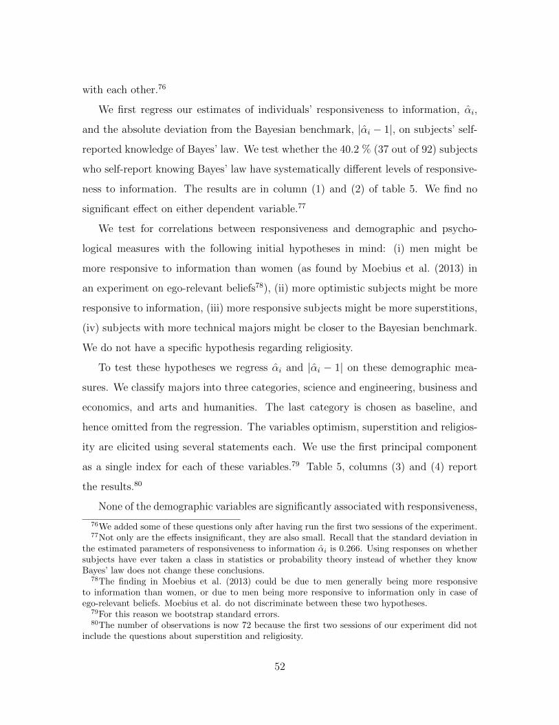
with each other.76

We first regress our estimates of individuals’ responsiveness to information, αi,

and the absolute deviation from the Bayesian benchmark, |αi − 1|, on subjects’ self-

reported knowledge of Bayes’ law. We test whether the 40.2 % (37 out of 92) subjects

who self-report knowing Bayes’ law have systematically different levels of responsive-

ness to information. The results are in column (1) and (2) of table 5. We find no

significant effect on either dependent variable.77

We test for correlations between responsiveness and demographic and psycho-

logical measures with the following initial hypotheses in mind: (i) men might be

more responsive to information than women (as found by Moebius et al. (2013) in

an experiment on ego-relevant beliefs78), (ii) more optimistic subjects might be more

responsive to information, (iii) more responsive subjects might be more superstitions,

(iv) subjects with more technical majors might be closer to the Bayesian benchmark.

We do not have a specific hypothesis regarding religiosity.

To test these hypotheses we regress αi and |αi − 1| on these demographic mea-

sures. We classify majors into three categories, science and engineering, business and

economics, and arts and humanities. The last category is chosen as baseline, and

hence omitted from the regression. The variables optimism, superstition and religios-

ity are elicited using several statements each. We use the first principal component

as a single index for each of these variables.79 Table 5, columns (3) and (4) report

the results.80

None of the demographic variables are significantly associated with responsiveness,

76We added some of these questions only after having run the first two sessions of the experiment.77Not only are the effects insignificant, they are also small. Recall that the standard deviation in

the estimated parameters of responsiveness to information αi is 0.266. Using responses on whethersubjects have ever taken a class in statistics or probability theory instead of whether they knowBayes’ law does not change these conclusions.

78The finding in Moebius et al. (2013) could be due to men generally being more responsiveto information than women, or due to men being more responsive to information only in case ofego-relevant beliefs. Moebius et al. do not discriminate between these two hypotheses.

79For this reason we bootstrap standard errors.80The number of observations is now 72 because the first two sessions of our experiment did not

include the questions about superstition and religiosity.

52

as column (3) shows. Turning to psychological variables, we find the expected positive

correlation of optimism with responsiveness. This effect, however, is not robust to

excluding religiosity from the regression equation (not reported).

Reassuringly, none of the demographic and psychological variables explain sub-

jects’ deviation from the Bayesian benchmark–all slope coefficients in column (4) are

statistically insignificant and small relative to the mean of the dependent variable

(0.215).

Finally, we consider the explanatory power of the demographic and psychological

variables in the Information Valuation and Gradual Information Tasks. We regress

∆vI,i and ∆bI,i on these variables, paralleling the analyses in sections 5.2 and 5.4.81

Again, demographic and psychological variables lack significant explanatory power.

The R2-coefficient of 8.8% of this regression does not compare favorably with the

R2-coefficient of 19.4% we obtain using (only) responsiveness to information as an

explanatory variable.82 Race has some explanatory power in the Gradual Information

Task.

We summarize these findings in the following result.

Result 6.

(i) Self-reported knowledge of Bayes’ law explains neither subjects’ responsiveness

to information nor subjects’ deviation from the Bayesian benchmark.

(ii) Demographic and psychological variables are not significantly related to subjects’

responsiveness to information or to subjects’ deviation from the Bayesian bench-

mark.

(iii) Demographic and psychological variables have lower explanatory power than re-

sponsiveness in the Information Valuation Task.

81The estimates in column 6 are based only on the set of subjects who chose to bet on the stateof the world at least once in each round of the Gradual Information Task.

82See column 2 in table 3.

53

(1) (2) (3) (4) (5) (6)VARIABLES αi |αi − 1| αi |αi − 1| ∆vI,i ∆bI,i

Knows Bayes’ law 0.057 0.013 0.073 0.066 -0.004 -0.127(0.074) (0.054) (0.076) (0.070) (0.014) (0.543)

Male 0.088 -0.045 -0.010 0.142(0.067) (0.056) (0.020) (0.736)

Science or engineering major -0.079 -0.002 -0.001 0.0236(0.069) (0.059) (0.021) (0.985)

Business or economics major -0.053 -0.068 -0.014 -1.218(0.100) (0.086) (0.029) (1.152)

African-american -0.160 0.053 -0.063 3.087(0.188) (0.177) (0.073) (2.020)

Asian 0.023 -0.112 0.021 2.720(0.025) (0.079) (0.039) (1.943)

Caucasian 0.051 -0.068 0.043 2.869*(0.107) (0.069) (0.035) (1.743)

CRT 0.026 -0.019 0.017 0.149(0.034) (0.029) (0.011) (0.440)

LOTR 0.040** -0.012 -0.002 0.0141(0.018) (0.016) (0.006) (0.256)

Superstition -0.007 0.016 -0.005 -0.0335(0.027) (0.022) (0.008) (0.300)

Religiosity 0.076 0.018 -0.000 -0.153(0.057) (0.031) (0.008) (0.287)

Constant 1.111*** 0.247*** 0.954*** 0.248 -0.077** -3.047(0.087) (0.062) (0.171) (0.264) (0.036) (1.949)

Session and order fixed effects Yes Yes Yes Yes No No

Observations 92 92 72 72 719 120R-squared 0.081 0.106 0.338 0.250 0.088 0.165

Bootstrapped standard errors in parentheses*** p<0.01, ** p<0.05, * p<0.1

Table 5: Responsiveness to information and demographic and psychological vari-ables. The excluded category for major is humanities and social sciences. The ex-cluded category for race is other. Models (5) and (6) do not include session and orderfixed effects which would inflate R2.

54

-.12

-.09

-.06

-.03

0.0

3.0

6.0

9

a b c d e f g h i jInformation Structure

Deviation of empirical valuation from normative benchmark

S1

S2

A1

A2

S3

B1

A3

B2

S4

B3

.5.6

.7.8

.91

P("1

"|1)

.5 .6 .7 .8 .9 1P("0"|0)

Information Structures

Figure 7: Mean deviation of empirical valuation from benchmark valuation. Stan-dard errors clustered by subject.

B Robustness Checks

B.1 Analysis on the full sample

In this section we redo our analysis including all subjects and all sessions (with the

exception of the pilot session). Our results do not change qualitatively, but the cor-

relations we observe are weaker. This is expected, since we now include subjects that

we have previously classified as noisy. Estimated parameters of responsiveness con-

tinue to be significantly correlated with behavior in the Information Valuation Task.

In the Gradual Information Task responsiveness to information retains statistical

significance if we control for demographic variables.

Aggregate analysis Figure 7, suggests the findings that we have obtained in the

main text hold on the full sample: less informative information structures are over-

valued, more informative information structures are undervalued, information struc-

tures are undervalued on average, there are slight boundary effects, and there is no

discernible evidence of any effects of asymmetry. Formal analysis reported in table 6

confirms this.

We now perform the analysis of section 4.1 on the entire sample. We again find

55

(1) (2) (3) (4) (5) (6) (7)Info Structures [S] [S,A] [S,A] [S,B] [S,B] [S,A,B] [S,A,B]Dependent Var vI,i vI,i vI,i vI,i vI,i vI,i vI,i

vtheorI .594*** .616*** .618*** .655*** .491*** .677*** .603***(.0450) (.0439) (.0437) (.0406) (.0427) (.0386) (.0427)

Asymmetry -.0475 -.0237(.0295) (.0260)

Boundary .0273*** .0342***(.00843) (.00968)

Constant .268*** .248*** .249*** .231*** .271*** .208*** .260***(.0338) (.0326) (.0327) (.0323) (.0330) (.0305) (.0326)

Observations 571 1000 1000 1000 1000 1429 1429R-squared .186 .140 .141 .202 .207 .172 .177

Standard errors in parentheses. Clustered by subjects.Reported significance levels for vtheorI concern the hypothesis that this coefficient is 1.

*** p<0.01, ** p<0.05, * p<0.1

Table 6: Aggregate valuations of information structures.

positive and highly significant boundary effects as well as mixed evidence for asym-

metry effects. Testing for equality of coefficients of column (7) in tables 6 and 7 we

find coefficients on vI,i and asymmetry to be the same (p = 0.293 and p = 0.7041,

respectively). The constant term is significantly smaller with dependent variable vpredI,i

than with dependent variable vI,i, indicating a willingness to pay for information that

is too low conditional on own beliefs. We continue to find boundary effects that are

significantly larger with dependent variable vpredI,i than with dependent variable vI,i

(p < 0.001).

Individual analysis Including all subjects in the analysis does not change much

even for the statistically more demanding individual level analysis of section 5.2.

Surprisingly, including all subjects leaves the relative importance of responsiveness to

information almost unchanged: the R2 coefficient in equation (2) as a fraction of the

R2 coefficient in equation (3) is 86.4 % (the corresponding ratio on the sample used

56

(1) (2) (3) (4) (5) (6)Method OLS OLS OLS OLS IV IV

Dependent Var vI,i vI,i vpredI,i vpredI,i vI,i vI,i

vpredI,i .518*** .471*** .878** .984(.0666) (.0775) (.0507) (.0730)

vtheorI,i .770*** .613***(.0233) (.0280)

Asymmetry -.0719 -.0108 -.0131(.0279) (.0209) (.0335)

Boundary .0443*** .0687*** -.0336**(.0134) (.00770) (.0141)

Constant .341*** .373*** .170*** .276*** .0589 -.0118(.0549) (.0612) (.0213) (.0229) (.0389) (.0540)

Instrument vtheorI,i vtheorI,i

Observations 1429 1429 1429 1429 1429 1429R-squared .213 .222 .280 .316 .110 .0524

Standard errors in parentheses. Clustered by subjects.

Reported significance levels for vpredI concern the hypothesis that this coefficient is 1.*** p<0.01, ** p<0.05, * p<0.1

Table 7: Relationship between beliefs and valuations.

57

(1) (2) (3) (4) (5) (6)VARIABLES ∆vI,i ∆vI,i ∆vI,i ∆vI,i ∆vI,i ∆vI,i

∆vpredI,i 0.413*** 0.246*** 0.387*** 0.214***(0.083) (0.066) (0.092) (0.080)

∆vI(αi) 0.550*** 0.300*** 1.244 1.020(0.144) (0.146) (0.360) (0.359)

Constant -0.044*** -0.035*** -0.038*** -0.049*** -0.036*** -0.039***(0.008) (0.008) (0.008) (0.009) (0.008) (0.008)

Observations 1,429 1,429 1,429 1,119 1,119 1,119R-squared 0.116 0.113 0.130 0.056 0.093 0.10710 percent trim no no no yes yes yes

Bootstrapped standard errors in parentheses84

*** p<0.01, ** p<0.05, * p<0.1Significance levels on the slope parameters concern the hypothesis that the coefficients are 1.

Table 8: Explaining and decomposing deviations from benchmark valuations.

in the main text is 85.1 %).83 This suggests that responsiveness to information is a

robust predictor of behavior, particularly in cases where behavior is noisy.

Including all subjects increases the noise to an overwhelming level in the Gradual

Information Task, however. While we still find the expected signs of the coefficients,

these are no longer significant, and the R2 coefficient drop to negligible levels. We

recover significance of responsiveness to information on the entire sample when we

control for covariates. Table 5, column (6), indicates that race is a strong predictor of

behavior in the Gradual Information Task. We include this variable in the regressions

corresponding to column (1) of table 9 and find responsiveness to information to be

a highly significant predictor of behavior.

83A slight increase occurs for equations (5) and (6) where the corresponding ratio changes from76.4 % to 87.0 %.

58

(1) (2) (3) (4)VARIABLES ∆bI,i ∆bI,i ∆bI,i ∆bI,i

αi -0.417 -1.017**(0.705) (0.501)

∆bI(αi) 0.138 1.580(0.318) (1.675)

Constant 0.281 2.428*** 2.297*** -1.168(0.774) (0.450) (0.774) (1.034)

Control for race no no no yesMethod OLS Tobit Tobit OLSObservations 172 432 344 17210-percent trim no no yes noR2 / pseudo-R2 0.009 0.005 0.018 0.179

Bootstrapped standard errors in parentheses.*** p<0.01, ** p<0.05, * p<0.1

Table 9: Predicting behavior in the gradual information task. Model (1) excludesall subjects with a censored observation. Model (2) includes all subjects and ob-servations. Model (3) excludes the subjects with parameters αi more extreme thanthe 10th or 90th percentile. Model (4) is model (1) with race-dummies as controlvariables.

59

B.2 Truncation in the aggregate analysis

Our result that subjects overvalue the less informative information structures and

undervalue the more informative ones might be a statistical artifact: First, it is

impossible to enter valuations that exceed one, and second, even for subjects who

do not know how to value a particular information structure, it might be obvious

that stating valuations short of 0.5 is suboptimal. Consequently, large upward errors

are possible for less informative information structures, but not for more informative

ones, and the opposite holds for large downward errors.

We show that our result is not a statistical artifact, as follows. If for information

structure I, the maximal upwards deviation from the theoretical valuation is M ,

then we set all valuations with vI,i < vtheorI −M equal to vtheorI −M . Similarly, if

the maximal downwards deviation from the theoretical valuation is m, then we set

all valuations with vI,i > vtheorI + m equal to vtheorI + m. We perform the analysis of

section 4 on this data. Table 10 displays the results.

Note that if the overweighting/underweighting effect is purely a statistical artifact,

then the coefficient on vtheorI will be equal to 1 in this procedure. On the other hand, if

the true coefficient on vtheorI is less than 1, then this procedure will bias the coefficient

estimates upwards.

We find that the overweighting / underweighting effect is reduced, but remains

substantial and highly statistically significant. Our conclusions regarding the bound-

ary and asymmetry effects are not substantially changed.

B.3 Framing effects and extremeness-avoidance

There are a variety of reasons that, in principle, could explain the consistency of

responsiveness to information. On the one hand, some people might be more prone

than others to avoid ‘extreme’ lines in the multiple price list, or they might have a

preference for playing the exogenous lottery to being paid according to the evaluation

option in each multiple price list. These effects are present to equal extents in both

60

(1) (2) (3) (4) (5) (6) (7)Info Structures [S] [S,A] [S,A] [S,B] [S,B] [S,A,B] [S,A,B]Dependent Var vI,i vI,i vI,i vI,i vI,i vI,i vI,i

vtheorI .844*** .840*** .842*** .879*** .840*** .887*** .829***(.0249) (.0264) (.0266) (.0223) (.0249) (.0239) (.0248)

Asymmetry -.0448* -.0256(.0256) (.0230)

Boundary .0167** .0273***(.00637) (.00668)

Constant .107*** .105*** .107*** .0864*** .111*** .0745*** .115***(.0213) (.0227) (.0225) (.0211) (.0222) (.0229) (.0219)

Observations 367 643 643 643 643 919 919R-squared .597 .448 .449 .608 .612 .511 .516

Standard errors in parentheses. Clustered by subjects.Reported significance levels for vtheorI concern the hypothesis that this coefficient is 1.

*** p<0.01, ** p<0.05, * p<0.1

Table 10: Results of section 4 correcting for truncation.

the belief updating task and the probability assessment task. On the other hand,

subjects might be influenced by the different numbers of black and white balls they

were presented with in part 1.

Our conclusions are robust to controlling for these effects. We perform the follow-

ing procedure. We first regress ∆vI,i on all ∆PI,i(“σ”), and on the sequence of balls

drawn in part 1. We then obtain the residuals from these regressions. We do the

same with the belief updating data. We calculate the Cronbach alpha coefficients of

the residuals to demonstrate consistency within parts of the experiment. To demon-

strate the explanatory power of responsiveness to information across parts, we regress

subjects’ mean residuals of the valuation data on their mean residuals from the belief

updating data. We do not apply such a procedure to the Gradual Information Task,

since there exists no obvious confound that would be common to both the Belief

Updating Task and the Gradual Information Task.

61

Formally, the first stage regression is,85

∆xI,i = βx0,I +10∑I′=1

[βxI′,I∆Pi,I′(“1”) + γxI′,I∆Pi,I′(“0”)

]+

6∑k=1

cki + εxI,i (10)

where cki is the color of the ball that subject i saw in round k of part 1, the εxI,i are

assumed to be i.i.d. with mean zero and x ∈ {v, P (1|“1”), P (0|“0”)} is one of our

behavioral variables of interest. We include session and order fixed-effects, and denote

the estimated residuals by εxI,i.

This model is the most general model with the properties that (i) the function

relating behavior in the Probability Assessment Task to behavior in a given other

part of the experiment is the same for all subjects and (ii) this function is linear. In

particular, it allows for each δxI,i to depend differentially on all of the δP (“σ”)i,I′ . Thus it

accommodates explanations such as people placing a constant premium (heterogenous

across individuals) on the exogenous lottery relative to the evaluation option or ideas

such as some people being more prone to avoid extreme lines in the multiple price

lists.

The Cronbach alpha coefficients of the residuals εvI,i, εP (1|“1”)I,i , and ε

P (0|“0”)I,i are

0.808, 0.814 and 0.706, respectively. These are slightly lower than the coefficients

obtained on the original data, but (with the exception of εP (0|“0”)I,i ) still compare favor-

ably with the standard benchmark of 0.8. Hence we still find consistent heterogeneity

in behavior within parts of our experiment.

To assess consistency across parts of the experiment, we define ηvi = 17

∑I∈S∪B ε

vI,i

and ηpi = 114

∑I∈S∪B ε

P (1|“1”)I,i + ε

P (0|“0”)I,i .86 We then regress ηvi on ηpi . We estimate a

slope coefficient of 0.134∗∗∗ (s.e. 0.023) and intercept coefficient of 0.000 (s.e. 0.005).

The R2 coefficient of this regression is 28.2 %.

85We randomly decided whether to elicit the probabilities of white or black balls. Hence either∆Pi,I′(“1”) = 0 or ∆Pi,I′(“0”) = 0 for each observation (i, I). We allow the parameters in the firststage regression to differ depending on whether we elicited the probability of a black ball or theprobability of a white ball to allow for the greatest generality.

86We exclude the boundary information structures.

62

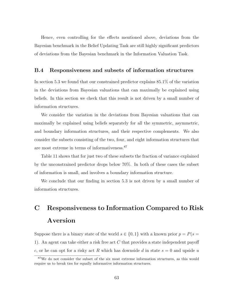
Hence, even controlling for the effects mentioned above, deviations from the

Bayesian benchmark in the Belief Updating Task are still highly significant predictors

of deviations from the Bayesian benchmark in the Information Valuation Task.

B.4 Responsiveness and subsets of information structures

In section 5.3 we found that our constrained predictor explains 85.1% of the variation

in the deviations from Bayesian valuations that can maximally be explained using

beliefs. In this section we check that this result is not driven by a small number of

information structures.

We consider the variation in the deviations from Bayesian valuations that can

maximally be explained using beliefs separately for all the symmetric, asymmetric,

and boundary information structures, and their respective complements. We also

consider the subsets consisting of the two, four, and eight information structures that

are most extreme in terms of informativeness.87

Table 11 shows that for just two of these subsets the fraction of variance explained

by the unconstrained predictor drops below 70%. In both of these cases the subset

of information is small, and involves a boundary information structure.

We conclude that our finding in section 5.3 is not driven by a small number of

information structures.

C Responsiveness to Information Compared to Risk

Aversion

Suppose there is a binary state of the world s ∈ {0, 1} with a known prior p = P (s =

1). An agent can take either a risk free act C that provides a state independent payoff

c, or he can opt for a risky act R which has downside d in state s = 0 and upside u

87We do not consider the subset of the six most extreme information structures, as this wouldrequire us to break ties for equally informative information structures.

63

Subset R2constrained/R

2both Subset R2

constrained/R2both

S 76.7% A,B 90.3%A 99.0% S,B 79.4%B 65.4% S,A 88.5%

S1, B3 45.1% S2, S3, B1, B2, A 95.9%S1, S2, B2, B3 70.3 % S2, S3, B1, B2, A 94.9%

S1, S2, S4, A,B2, B3 82.4 % S3, B1 92.6%

Table 11: Fraction of explainable variance in individual biases in valuations thatcan be explained using responsiveness alone, on subsets of information structures.R2constrained is the R2 of a regression of ∆vI,i on the constrained predictor. R2

both is theR2 of a regression of ∆vI,i on both the constrained and the unconstrained predictor.

in state s = 1, where d < c < u, as depicted in the following table.

Act s = 0 s = 1

C c c

R d u

Before making a decision, the agent has the opportunity to acquire a costly infor-

mative signal “σ” ∈ {“0”, “1”} about the state of the world. We are interested in the

comparative statics of the agent’s willingness to pay for the information with respect

to (i) his responsiveness to information and (ii) his risk aversion.

It is clear that the agent’s willingness to pay for information is increasing in his

responsiveness to information, regardless of which act he would choose in the absence

of information. This is because an agent who is more responsive to information

experiences a greater reduction in subjective uncertainty upon observing any signal.

Importantly, however, the comparative statics with respect to risk aversion depend

on what action the agent would take in the absence of information.

First, suppose that the parameters of the problem are such that in the absence of

information the agent chooses the risky act R. In this case, a signal realization either

increases the subjective probability for s = 1, in which case the agent also decides

for the risky act after observing the signal. Or it decreases the subjective probability

for s = 1, in which case the agent might opt for the riskless act C instead. Hence,

64

information can prevent the agent from deciding for R when doing so would likely

pay the downside d.88 An increase in risk aversion decreases the attractiveness of R

for any posterior about s, but leaves the attractiveness of C unchanged. Therefore, a

more risk averse agent who, in the absence of information, opts for the risky option

has more to gain from information. Hence, his willingness to pay for information

increases with risk aversion.

Second, suppose that the parameters of the problem are such that in absence

of information, the agent would instead optimally choose the riskless act C. Now,

if the signal realization decreases the subjective probability that s = 1, then the

agent still opts for the riskless act C. If it increases the subjective probability that

s = 1, however, the agent might choose the risky act R instead. Hence, information

can help the agent to take the risk R when doing so is likely to pay the upside u.89

Now, an increase in risk aversion decreases the attractiveness of the risky option R

relative to the riskless option C. Hence, a more risk averse agent has less to gain

from information. Consequently, if in the absence of information the agent opts

for the riskless option, an increase in risk aversion decreases willingness to pay for

information.90

88Conditional on this signal, EU(R) < EU(C).89Conditional on this signal, EU(R) > EU(C).90We can use this simple model to derive predictions of individual behavior across markets for

information. Suppose that market A provides information for decisions in which people by defaultopt for the risky option, whereas market B provides information for decisions in which people usuallyopt for the riskless option. If people are all similarly risk averse but heterogenous in responsivenessto information, then individuals’ willingness to pay for information is positively correlated acrossthe two markets. On the other hand, if people are all similarly responsive to information but differin risk aversion, we expect negative correlation between individual willingness to pay across marketsA and B.

65

D Experimental Instructions

66

WELCOME!!!This is a study of individual decision-making and behavior. Money earned will be paid to you in cash at the end of this experiment. !!In addition to your $5 show up payment and your $15 completion payment, you will be paid in cash your earnings from the experiment. This experiment proceeds in 5 parts. For each part, we will give you instructions just before that part begins. Your choices in one part of the experiment will not affect what happens in any other part. Each part proceeds in rounds. In total, there will be 40 rounds of similar length and an additional 40 rounds of shorter length. The experiment will end with a short questionnaire, for which you may earn additional money. After you are finished with the experiment, we will draw one of the parts of the experiment at random, and one of the rounds within this part, so that each round of the experiment is similarly likely to be drawn. We will pay you in cash for the decision that you made in that round (the Payment Round), and only in that round. Hence you should make every decision as if it is the one that counts, because it might be! Remember that this is a study of individual decision-making, which means you are not allowed to talk during the study. If you have any questions, please raise your hand and we will come and answer your questions privately. Please do not use cell phones or other electronic devices until after the study is over. If we do find you using your cell phone or other electronic devices, the rules of the study require us to withhold your completion payment. Often during this study, you will be shown information or asked to make decisions. After doing so, remember to click the button that says “Continue” or “Save My Decisions”. The experiment will not proceed until you click that button.

PART 1

The first part of the experiment proceeds in 6 rounds. In each round, you will play the Prediction Game (described below), for a prize of $35. In each round there are two boxes, Box X and Box Y. Each of the boxes contains balls that are either black or white. Box X contains 10 balls. Box Y contains 20 balls. For example, Box X could contain 7 black balls and 3 white balls, and Box Y could contain 14 white balls and 6 black balls. The composition of the boxes may change from round to round.

THE PREDICTION GAME At the beginning of the Prediction Game, the computer will select either Box X or Box Y by tossing a fair coin. Thus, Box X is selected with chance 50%, and Box Y is selected with chance 50%. The box that has been selected is called the Selected Box. We will not tell you which box has been selected by the computer.

The computer will then draw a ball randomly from the Selected Box, and show that ball to you. Your task is to predict whether the Selected Box is Box X or Box Y. If you predict correctly, you will receive $35. If you predict incorrectly, you will receive $0.

For instance, suppose you predict that the Selected Box is Box X. Then you get $ 35 if the Selected Box is in fact Box X.

We will not tell you whether your prediction was correct until the end of the experiment. The flow chart on the next page illustrates what happens in the Prediction Game.

This may seem simple, but we just want you to get used to playing this game.

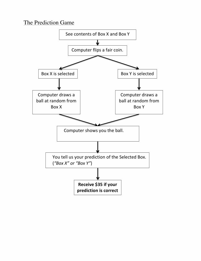
The Prediction Game

Computer!flips!a!fair!coin.!

Box!X!is!selected! Box!Y!is!selected!

Computer!draws!a!ball!at!random!from!

Box!X!

Computer!draws!a!ball!at!random!from!

Box!Y!

You!tell!us!your!prediction!of!the!Selected!Box.!(“Box%X”%or%“Box%Y”)!

Receive&$35&if&your&prediction&is&correct&

Computer!shows!you!the!ball.!

See!contents!of!Box!X!and!Box!Y!

PART 2

This part of the experiment proceeds in 10 rounds. In each round, we will show you two boxes, Box X and Box Y. We then ask whether you would rather play the Prediction Game with those boxes, for a prize of $35, or instead have a stated chance of winning of $35. After inspecting the boxes, you will make a choice by filling in a list such as this:

At the end of the experiment, the computer will select one of the lines on this list at random. That decision will be the one that counts. All numbers that you see in this part of the instructions are chosen to illustrate the payment procedure. These numbers will not be relevant once we start this part of the experiment.

For instance, suppose that you filled in the list like this:

Suppose that the computer selects the third line from the top. On this line, you ticked the option on the right. Hence you will receive $35 with chance 94 %, and $0 otherwise. Suppose instead that the computer selects the fifth line from the top. On this line, you ticked the option on the left. Hence, you will play the prediction game. Your task is to consider, for each line, whether you would rather play the Prediction Game with the boxes offered, or instead receive $35 with the chance on the right. If you prefer playing the prediction game to getting $35 with chance 12%, for instance, then you will also prefer playing the prediction game to getting $35 with any lower chance. Similarly, if you prefer getting $35 with chance 13% to playing the prediction game, then you will also prefer getting $35 with any chance higher than 13% to playing the prediction game. For your convenience, once you tick a given option, the computer will fill in the lines above and below in this way.

Our payment procedure is designed so that it is in your best interest to choose on each line the option you genuinely prefer. At the end of the experiment, what happens if a round from this part is the one selected as the Payment Round? The computer will select a line from your choice list for that round. If, on that line, you chose to play the Prediction Game for a $35 prize, then you will play the Prediction Game with the boxes from that round. If, on that line, you chose to have a chance of receiving $35, then you will receive $35 with the specified chance. Specifically, you will be shown a wheel of luck. The wheel is part green and part red. The fraction of the wheel of luck that is green is exactly the specified chance of getting $35, the remaining part of the wheel is red. You will click a button to spin the needle. You will get $35 if the needle stops on the green part of the wheel, and you will get $0 if the needle stops on the red part of the wheel. You may change your decisions as many times as you like. Your decisions are final as soon as you click the SAVE MY DECISIONS button. Once at least 10 seconds have passed and you have made all your decisions, this button will automatically appear on the bottom of your screen.

PART 3

This part of the experiment proceeds in 10 rounds. In each round, we will show you two boxes, Box X and Box Y. The computer will select a Box using the flip of a fair coin, and draw a ball randomly from that Box. We will not tell you the color of the ball yet. In each round, we ask you to assess:

1. If the ball is BLACK, how likely it is that the ball was drawn from BOX X. 2. If the ball is WHITE, how likely it is that the ball was drawn from BOX Y.

After inspecting the boxes, you will fill in two lists such as these:

If this round is chosen for payment, the computer will draw a ball at random from the selected box. If the ball is BLACK, the computer will select a line at random from the first list, and carry out your stated choice. If the ball is WHITE, the computer will select a line at random from the second list, and carry out your stated choice. All the numbers that you see in this part of the instructions are chosen to illustrate the payment procedure. These numbers will not be relevant once we start this part of the experiment. For instance, suppose the ball is White. Also suppose that the computer selects the fourth line from the bottom of the second list. If you chose the option “get $35 if the Selected Box is Box Y”, then you will receive $35 if and only if the selected box is Box Y. If you chose the option “get $35 with chance 10%”, then you will receive $35 with chance 10%. How should you decide which options to tick? That depends on how likely you think that, given the drawn ball is white, the Selected Box is Box Y. Suppose you think there is a 63% chance of this. Then you should tick the LEFT option on any line where the RIGHT option offers you a smaller than 63% chance of a cash prize. And you should tick the RIGHT option on any line where the RIGHT option offers you a greater than 63% chance of a cash prize. Suppose you instead ticked the Left Option for all chances less than 90%, and the Right Option for all chances greater than 90%. If the computer selects one of the lines between 63% and 90%, then you will be given the Left Option (which you believe yields a payment 63% of the time) instead of the Right Option, which yields a payment more than 63% of the time! Suppose instead you ticked the left option for all chances less than 30%, and the right option for all chances greater than 30%. If the computer selects one of the lines between 30% and 63%,

then you will be given the Right Option (which yields a payment less than 63% of the time), instead of the Left Option, which you believe yields a payment 63% of the time! Thus, our payment procedure is designed so that your earnings are highest if you provide your most accurate estimate. The box letters and ball colors that we are asking about will change from round to round. The flow chart below illustrates what happens in one round.

Computer!flips!a!fair!coin.!

Box!X!is!selected! Box!Y!is!selected!

Computer!draws!a!ball!at!random!from!

Box!X!

Computer!draws!a!ball!at!random!from!

Box!Y!

Black!Ball?! White!Ball?!

Computer!picks!a!random!line!from!the!“If!Black”!list!

!

Computer!picks!a!random!line!from!the!“If!White”!list!

!

Your&choice&from&that&line&is&carried&

out.!!

Your&choice&from&that&line&is&carried&

out.!!

PART 4

This part of the experiment proceeds in 10 rounds. In each round, we will show you two boxes, Box X and Box Y. The computer will select a Box using the flip of a fair coin, and draw a ball randomly from that Box. In this part of the experiment, we ask you to assess how likely it is that the drawn ball is Black or White. You will make a choice by filling in a list such as this:

As before, the computer will randomly select a line from the list, and carry out the choice that you made in that line.

All the numbers that you see in this part of the instructions are chosen to illustrate the payment procedure. These numbers will not be relevant once we start this part of the experiment. How should you decide which options to tick? That depends how likely you think it is that the drawn ball is black. For instance, if you think that there is a 70% chance that the drawn ball is black, then you should tick the LEFT option on any line where the RIGHT option offers you less than a 70% chance of a cash prize, and you should tick the RIGHT option on any line where the RIGHT option offers you a greater than 70% chance of a cash prize. You may change your decisions as many times as you like. Your decisions are final as soon as you click the SAVE MY DECISIONS button. Once at least 10 seconds have passed and you have made all your decisions, this button will automatically appear on the bottom of your screen. Remember, our payment procedure is designed so that your earnings are highest if you provide your most accurate estimate. The ball color that we are asking about will change from round to round.

PART 5

This part of the experiment proceeds in 4 blocks. Each block has 12 rounds. In each block, we will show you two boxes, Box X and Box Y. Each contains 20 balls. For instance, Box X could contain 12 black balls and 8 white balls. Box Y could contain 12 white balls and 8 black balls.

At the start of each block, this is what will happen:

1. You will be shown the contents of the two boxes for the current block 2. The computer will select a Box by flipping a fair coin. This Box will remain the same

for the entire block. During the 12 rounds of a block, this is what will happen in each round:

1. The computer will draw a ball at random from the Selected Box and show it to you 2. You can then choose one of the following three options:

3. The computer will put the ball back in the selected box.

Note that the Selected Box stays the same for the entire 12 rounds of the block. A new Selected Box will be drawn only at the beginning of each block. Payment If the computer chooses this part of the experiment for payment, here's what will happen. The computer randomly chooses a block, and a round within this block. The computer will then carry

out the choice you made in this round. That is, if you chose the option on the left, you will get $ 35.- if the Selected Box in this block was indeed Box X; if you chose the middle option, you will get $ 35.- with the specified chance; and if you chose the option on the right, you will get $ 35.- if the Selected Box was indeed Box Y. Please note the following:

• The chance with which you can receive $ 35.- if you choose the middle option may vary from block to block. But it will stay the same for all 12 rounds within a block.

• A new Selected Box is drawn at the beginning of each block, and will stay the same for all 12 rounds within the block.

• After a ball has been drawn from the Selected Box, it is put back into the Selected Box. Hence, draws are with replacement.

& &

Overview&of&part&5&

!BLOCK&1& &!You!see!the!contents!of!Box!X!and!Box!Y!!Computer!draws!the!Selected!Box.!!! !Round!1! (i)!Computer!draws!a!ball!from!the!Selected!Box!and!shows!it!to!you!! (ii)!You!choose!between!the!left,!middle,!or!right!options!! (iii)!Computer!returns!the!ball!to!the!Selected!Box!! !Round!2! like!round!1!!...!!Round!12! like!round!1!!!BLOCK&2& &! !You!see!the!contents!of!Box!X!and!Box!Y!!Computer!draws!the!Selected!Box.!!! !Round!1! (i)!Computer!draws!a!ball!from!the!Selected!Box!and!shows!it!to!you!! (ii)!You!choose!between!the!left,!middle,!or!right!options!! (iii)!Computer!returns!the!ball!to!the!Selected!Box!! !Round!2! like!round!1!!...!!Round!12! like!round!1!!!BLOCK&3&like!block!2! &&!BLOCK&4&like!block!2! &

QUESTIONNAIRE

Thank you for participating in the experiment! We would like to ask you a few questions about yourself. At the end of the questionnaire, the computer will randomly select a round, and a decision that you made in that round. We will pay you in cash for that decision. If the decision selected was from Part 2, and you chose to play the Prediction Game, then you will play a final round of the Prediction Game, with the relevant boxes displayed. This will be for a cash prize of $35.