behaviour of ferrocement columns under static and cyclic

Behaviour of ferrocement columns

under static and cyclic loading

A thesis submitted to The University of Manchester for the degree of

Doctor of Philosophy

in the Faculty of Engineering and Physical Sciences

2013

Jianqi Wang

BEng, MSc

SCHOOL OF MECHANICAL, AEROSPACE AND CIVIL

ENGINEERING

1

DECLARATION

No portion of the work referred to in this dissertation has been submitted, in support

of an application, for another degree or qualification of this or any other university

or institution of learning.

Jianqi Wang

2

ACKNOWLEDGEMENTS

I would like to thank Parthasarathi Mandal and Paul Nedwell for their excellent

supervision, valuable guidance, constructive discussions and encouragement

throughout the period my research at Manchester.

I would also like to thank John Mason, David Mortimer, Shichuan Tian, Lu Chen

and Chao Han for their generous help with the experiment tests in this dissertation

study.

Finally, I would like to thank my family for their moral support and their

encouragement throughout my studies.

3

COPYRIGHT STATEMENT

i. The author of this thesis (including any appendices and/or schedules to this thesis)

owns any copyright in it (the “Copyright”) and he has given The University of

Manchester the right to use such Copyright for any administrative, promotional,

educational and/or teaching purposes.

ii. Copies of this thesis, either in full or in extracts, may be made only in accordance

with the regulations of the John Rylands University Library of Manchester. Details

of these regulations may be obtained from the Librarian. This page must form part of

any such copies made.

iii. The ownership of any patents, designs, trademarks and all other intellectual

property rights except for the Copyright (the “Intellectual Property Rights”) and any

reproductions of copyright works, for example graphs and tables (“Reproductions”),

which may be described in this thesis, may not be owned by the author and may be

owned by third parties. Such Intellectual Property Rights and Reproductions cannot

and must not be made available for use without the prior written permission of the

owner(s) of the relevant Intellectual Property Rights and/or Reproductions.

iv. Further information on the conditions under which disclosure, publication and

commercialisation of this thesis, the Copyright and any Intellectual Property and/or

Reproduction described in it may take place is available in the University IP Policy,

in any relevant Thesis restriction declarations deposited in the University Library,

The University Library’s regulations and in the University’s policy on Presentation

of Thesis.

4

ABSTRACT

This thesis presents the results of an experimental, numerical and analytical study to

develop a design method for ferrocement columns and reinforced concrete columns

strengthened using ferrocement jackets. Two groups tests were conducted,

comprising five static loading tests and three cyclic load tests. The static tests had

one reinforced concrete column, two ferrocement columns and two strengthened

reinforced concrete columns. The cyclic loading tests were conducted on one

reinforced concrete column and two ferrocement columns. For both sets of tests, the

loading applications included two steps, first axial load and then lateral load.

The experimental data were used for validation of the finite element models that

were developed using the ABAQUS software package. The validated models were

used as part of a comprehensive parametric study to investigate the effects of a

number of design parameters including the effects of material strength,

reinforcement geometry and arrangement, and the influence of the axial load.

The main conclusions from the experiments and the parametric studies were that the

number of layers of mesh in the ferrocement has a significant effect on the peak

lateral load capacity of a column and ferrocement can be used as a strengthening or

retrofitting material. Based on the results from the experimental and numerical

studies, it was observed that the existing design methods significantly underestimate

the peak lateral load capacity.

It is found that the ACI design guideline for ferrocement columns is conservative

because the transverse wires in the ferro-mesh provide confinement. The ferro-mesh

transverse direction has very fine wire as confinement. Therefore, ferrocement has a

high potential for use as a repair/strengthening material. The detailed parametric

study data was condensed into a dimensionless interaction diagrams that can be used

for the design of new ferrocement columns as well as strengthening of reinforced

concrete columns using ferrocement jackets.

5

CONTENT

DECLARATION ....................................................................................................... 1

ACKNOWLEDGEMENTS ...................................................................................... 2

COPYRIGHT STATEMENT .................................................................................. 3

ABSTRACT ............................................................................................................... 4

CONTENT ................................................................................................................. 5

LIST OF FIGURES ................................................................................................ 11

LIST OF TABLES .................................................................................................. 18

LIST OF NOTATIONS .......................................................................................... 20

CHAPTER 1 INTRODUCTION ....................................................................... 24

1.1 Background ............................................................................................... 24

1.2 Aims and objectives .................................................................................. 26

1.3 Organization of the thesis.......................................................................... 27

CHAPTER 2 FERROCEMENT: MATERIAL BEHAVIOUR AND

APPLICATIONS .................................................................................................... 29

2.1 Ferrocement: definition and history .......................................................... 29

2.2 Application of ferrocement ....................................................................... 32

2.3 Constituent materials ................................................................................. 34

2.3.1 Matrix ..........................................................................................................34

2.3.1.1 Cement ................................................................................................................34 2.3.1.2 Aggregates ..........................................................................................................34 2.3.1.3 Water ..................................................................................................................35 2.3.1.4 Admixtures ..........................................................................................................35

2.3.2 The property of the matrix ...........................................................................36

2.3.3 Reinforcement mesh ....................................................................................36

2.4 Reinforcement mesh parameters ............................................................... 38

2.5 Behaviour of ferrocement ......................................................................... 41

2.5.1 Behaviour under tension ..............................................................................41

2.5.2 Behaviour under compression......................................................................43

2.5.3 Behaviour under flexure ..............................................................................44

2.5.4 Behaviour under shear .................................................................................46

2.6 Ferrocement as repair or strengthening material ....................................... 47

6

2.7 Theoretical study of reinforced concrete under combined uniaxial bending

and axial load ........................................................................................................ 48

2.8 Experimental studies of columns under bending and axial load ............... 53

2.8.1 Reinforced concrete columns .......................................................................53

2.8.2 Ferrocement columns ...................................................................................54

2.8.3 Reinforced concrete columns strengthened using ferrocement jacket .........54

2.9 FEM in ferrocement research .................................................................... 55

2.10 Ductility .................................................................................................... 56

2.11 Cyclic load effect on ferrocement structures ............................................ 59

2.12 Summary and conclusions ........................................................................ 60

CHAPTER 3 EXPERIMENTAL TESTS ......................................................... 61

3.1 Introduction ............................................................................................... 61

3.2 Material property tests: concrete and matrix ............................................. 61

3.2.1 Experiment preparation ................................................................................61

3.2.2 Sampling ......................................................................................................63

3.2.3 Specimen tests ..............................................................................................64

3.2.3.1 Compressive test: ...............................................................................................64 3.2.3.2 Split test: .............................................................................................................65

3.2.4 The test results .............................................................................................66

3.3 Reinforcing material tests ......................................................................... 67

3.4 Column Specimens ................................................................................... 69

3.5 Casting ...................................................................................................... 71

3.5.1 The concrete columns (RC) .........................................................................71

3.5.2 The ferrocement columns (FC) ....................................................................74

3.5.3 Reinforced concrete column strengthened using ferrocement jacket (RFC) ..

.....................................................................................................................78

3.6 The experimental rig ................................................................................. 82

3.6.1 The methodology .........................................................................................82

3.6.2 The position of the linear potentiometers ....................................................87

3.6.3 The loading frame ........................................................................................89

3.7 Specimen set up and load application ....................................................... 92

3.7.1 Axial load application ..................................................................................92

3.7.2 Lateral load application................................................................................94

7

3.8 Summary ................................................................................................... 95

CHAPTER 4 EXPERIMENTAL RESULTS ................................................... 97

4.1 Introduction ............................................................................................... 97

4.2 Initial displacement results ........................................................................ 97

4.3 The displacement at the top of the fixed-end plate ................................... 98

4.4 Reinforced concrete column under static load ........................................ 102

4.5 Ferrocement column under static load .................................................... 106

4.6 Reinforced concrete column strengthened using ferrocement jacket under

static load ............................................................................................................ 110

4.7 Cyclic loading tests ................................................................................. 114

4.7.1 Load reduction ...........................................................................................114

4.7.2 Stiffness degradation ..................................................................................118

4.7.3 Failure of the specimens ............................................................................119

4.8 Deformation ductility results................................................................... 122

4.9 Summary and conclusion ........................................................................ 125

CHAPTER 5 FINITE ELEMENT MODELLING ........................................ 127

5.1 Introduction ............................................................................................. 127

5.2 Element type............................................................................................ 128

5.2.1 Solid element: concrete and matrix ............................................................128

5.2.2 Truss element: steel bar, stirrup and welded mesh ....................................129

5.3 Concrete damaged plasticity model ........................................................ 129

5.3.1 Concrete under uniaxial compression ........................................................129

5.3.2 Compressive behaviour for CDP ...............................................................131

5.3.2.1 Eurocode 2 concrete material model: ............................................................. 131 5.3.2.2 Popovics model for matrix material: ............................................................... 133

5.3.3 Concrete under uniaxial tension.................................................................135

5.3.4 Tensile behaviour for CDP ........................................................................137

5.3.5 Plasticity parameters for CDP model .........................................................139

5.3.5.1 Dilation angle (ψ) ............................................................................................ 141 5.3.5.2 Eccentricity ( ) ................................................................................................. 142 5.3.5.3 σbo/σco .............................................................................................................. 143 5.3.5.4 Kc ...................................................................................................................... 144 5.3.5.5 Viscosity parameter ......................................................................................... 145

5.4 Contact .................................................................................................... 147

8

5.4.1 Embedded region .......................................................................................147

5.4.2 Tie constraint .............................................................................................147

5.5 Boundary conditions and load application .............................................. 148

5.6 Detail description of reinforcement in ABAQUS ................................... 149

5.7 Finite element mesh size ......................................................................... 151

5.8 Verification of FEM with experiments ................................................... 154

5.8.1 Reinforced concrete column ......................................................................155

5.8.2 Ferrocement columns .................................................................................158

5.8.3 Reinforced concrete columns strengthened using ferrocement jackets .....162

5.9 Ductility of FEM compared with experimental tests .............................. 168

5.10 Conclusion .............................................................................................. 168

CHAPTER 6 PARAMETRIC STUDIES ....................................................... 170

6.1 Introduction ............................................................................................. 170

6.2 Parameters ............................................................................................... 170

6.3 Columns .................................................................................................. 171

6.3.1 End conditions ...........................................................................................171

6.3.2 Axial load ...................................................................................................172

6.3.3 Length ........................................................................................................176

6.4 Concrete strength .................................................................................... 177

6.5 Matrix strength ........................................................................................ 178

6.6 Main reinforcing bar ............................................................................... 179

6.6.1 Strength ......................................................................................................179

6.6.2 Diameter and number of bars .....................................................................180

6.7 Stirrups .................................................................................................... 183

6.7.1 Strength ......................................................................................................183

6.7.2 Size ............................................................................................................184

6.8 Welded mesh ........................................................................................... 185

6.8.1 Strength ......................................................................................................185

6.8.2 Diameter.....................................................................................................187

6.8.3 Number of layers .......................................................................................189

6.9 Summary ................................................................................................. 191

CHAPTER 7 DESIGN GUIDELINES ........................................................... 192

9

7.1 Introduction ............................................................................................. 192

7.2 Material property ..................................................................................... 192

7.2.1 Welded mesh property ...............................................................................192

7.2.2 Matrix property ..........................................................................................194

7.3 Theoretical interaction diagrams and FEM results ................................. 196

7.3.1 The simplified strain and stress distribution diagram of FC4 ....................196

7.3.2 Interaction diagram (P-M) for the matrix ..................................................199

7.4 Example calculation using FC4 .............................................................. 201

7.4.1 Information required ..................................................................................201

7.4.2 Point a: Pure moment .................................................................................203

7.4.3 Point b: Strength at the balanced condition ...............................................206

7.4.4 Point bc: M-ds12 mesh at zero tensile strain ...............................................208

7.4.5 Point c: Pure axial load: .............................................................................210

7.4.6 The interaction diagram of FC4 .................................................................211

7.5 Theoretical results ................................................................................... 212

7.6 Comparison of the theoretical interaction diagrams with ABAQUS ...... 215

7.7 Non-dimensional interaction diagrams ................................................... 218

7.8 Example for using the interaction diagram ............................................. 220

7.9 Ferrocement column guideline ................................................................ 222

7.10 Summary ................................................................................................. 226

CHAPTER 8 CONCLUSIONS AND RECOMMENDATIONS FOR

FUTURE STUDIES .............................................................................................. 227

8.1 Summary ................................................................................................. 227

8.1.1 Experimental results ..................................................................................227

8.1.2 Finite element modelling analysis and parametric studies .........................229

8.1.3 Design guide ..............................................................................................231

8.2 Conclusion .............................................................................................. 232

8.3 Recommendations for future study ......................................................... 232

REFERENCES ...................................................................................................... 234

APPENDIX A. REINFORCEMENT PROPERTIES ............................................................ 239

APPENDIX B. THE DIMENSIONS OF THE SPECIMENS ............................................... 241

APPENDIX C. THE SPECIMENS AFTER THE TESTS..................................................... 243

10

APPENDIX D. SUPPORT ROTATION AND BENDING-SHEAR EFFECT .................... 247

APPENDIX E. TEST RESULTS FOR ALL THE LINPOTS ............................................... 254

APPENDIX F. DUCTILITY CALCULATIONS ................................................................... 261

APPENDIX G. FULL DETAILS OF THE CHANGING PARAMETERS ......................... 266

APPENDIX H. FC2 AND FC4 AT DIFFERENT AXIAL LOADS ...................................... 269

APPENDIX I. EFFECTIVE ROTATIONAL STIFFNESS FOR SUPPORT CONDITION .......

............................................................................................................................... 270

11

List of Figures

Figure 2-1: Typical meshes used in ferrocement application ................................... 29

Figure 2-2 Examples of ferrocement applications, (a): (BSS, 2011), (b): (Cambodia,

2010), (c): (Nedwell, 2009), (d): (Ferrocement.com, 2009), (e): (jadferrocements.net,

2010), (f): (jadferrocements.net, 2010) ..................................................................... 33

Figure 2-3: Typical types of mesh, (a): (Woven-mesh), (b): (Welded-mesh)

(c): (Hexagonal-mesh) (d): (Expanded-mesh) .......................................................... 37

Figure 2-4: Proposed longitudinal and transverse directions of reinforcement mesh

(ACI, 1988) ............................................................................................................... 40

Figure 2-5: Ferrocement under tension (Naaman, 2000) .......................................... 42

Figure 2-6: Typical load-deflection response of ferrocement (Naaman, 2000) ........ 45

Figure 2-7: The beam section, strain diagram and stress/force diagram with neutral

axis in section (after ACI 318) .................................................................................. 49

Figure 2-8: The interaction diagram for the element under bending and axial loading

(Caprani, 2006) ......................................................................................................... 51

Figure 2-9: Deformation ductility on a general load-displacement curve (Barrera et

al., 2012).................................................................................................................... 59

Figure 3-1: Matrix mix in the blender ....................................................................... 63

Figure 3-2: Horizontal and vertical strain gauges, and the dental plaster ................. 64

Figure 3-3: The tensile test (a): jig with packing strips, (b): cylinder split test failure

................................................................................................................................... 65

Figure 3-4: Typical concrete cylinder compressive test of stress-strain curve ......... 66

Figure 3-5: Typical matrix cylinder compressive test of stress-strain curve ............ 67

Figure 3-6 Mesh tensile test set up ............................................................................ 68

Figure 3-7: Typical reinforcement properties from the experimental tests ............... 69

Figure 3-8 Relationship between the eight column specimens ................................. 70

Figure 3-9: Reinforcement arrangement in the concrete column.............................. 72

Figure 3-10: Reinforcing steel in a square oiled steel mould.................................... 73

Figure 3-11: The specimens ...................................................................................... 73

Figure 3-12: The pattern of 2 and 4 layers mesh in the ferrocement columns .......... 74

Figure 3-13: The ferrocement column skeleton and mould ...................................... 75

Figure 3-14: Mesh sheet roll ..................................................................................... 76

Figure 3-15: Mesh cutting ......................................................................................... 76

12

Figure 3-16: Mesh bending ....................................................................................... 77

Figure 3-17: The assembly of mesh layers with plastic ties ..................................... 78

Figure 3-18: The pattern of reinforced concrete strengthened with 2 and 3 layers

mesh .......................................................................................................................... 79

Figure 3-19: Preparation for strengthening ............................................................... 80

Figure 3-20: Casting the strengthened concrete column with ferrocement .............. 81

Figure 3-21: Reinforced concrete columns strengthen with ferrocement jackets ..... 81

Figure 3-22: The column design layout, and test design layout as a cantilever........ 82

Figure 3-23: Layout of the column setup .................................................................. 83

Figure 3-24: The design layout of the test setup (parts detail are shown in Table 3-4)

................................................................................................................................... 85

Figure 3-25 A column setup on the equipment before the test ................................. 86

Figure 3-26 The pin joint between actuator and thick steel plate ............................. 86

Figure 3-27: Dental plaster ....................................................................................... 87

Figure 3-28: Location of linpots under the specimen, (a): initial arrangement,

(b): final arrangement ................................................................................................ 88

Figure 3-29: Arrangement of linpots on the underside of the specimen ................... 88

Figure 3-30: The two extra linpots added at the top of the fixed-end area ............... 89

Figure 3-31: Loading frame layout ........................................................................... 90

Figure 3-32: Loading frame ...................................................................................... 91

Figure 3-33: The controller for both static and cyclic tests ...................................... 92

Figure 3-34: Extension bar and coupler .................................................................... 93

Figure 3-35: The hydraulic jack connection with the end of the Macalloy bar with an

extra bar ..................................................................................................................... 94

Figure 3-36: The strain gauge fixed at the middle of each Macalloy bar and the

connection with the strain indicator box ................................................................... 94

Figure 4-1: Load-displacement relationships for LiF1, LiB1, LiF4 and LiB4 (RC) 98

Figure 4-2: Load-displacement relationships for Li8, Li9 and best-fit linear curves 99

Figure 4-3: Simplified diagram of the specimen at the support end ....................... 100

Figure 4-4: Load-displacement curves at different positions (Initial column, RC) 103

Figure 4-5: Displacement for each linpot at different loads (Initial column, RC) .. 104

Figure 4-6: Load-displacement curves for the support rotation effect and the

bending-shear effect at Li-A (Initial column, RC) .................................................. 104

Figure 4-7: Load-displacement curves at Li-A (FC2 and FC4) .............................. 107

13


bending-shear effect at Li-A (FC2) ......................................................................... 108


bending-shear effect at Li-A (FC4) ......................................................................... 109

Figure 4-10: Load-displacement curves for the RC and strengthened RC columns

under static load at Li-A .......................................................................................... 111

Figure 4-11: Load-displacement curves for support rotation effect and bending-shear

effect at Li-A (RFC2) .............................................................................................. 112


effect at Li-A (RFC3) .............................................................................................. 113

Figure 4-13: Load-displacement curves for RC-C under cyclic load at Li-A......... 116

Figure 4-14: Load-displacement curves for FC2-C under cyclic load at Li-A ....... 116

Figure 4-15: Load-displacement curves for FC4-C under cyclic load at Li-A ....... 117

Figure 4-16: Load degradation against number of cycles (for details see Appendix E)

................................................................................................................................. 117

Figure 4-17: Stiffness degradation during number of cycles (for detail see

Appendix E) ............................................................................................................ 119

Figure 4-18: Load-displacement curves for RC-C after 600 cycles and RC at Li-A

................................................................................................................................. 120

Figure 4-19: Load-displacement curves for FC2-C after 600 cycles and static test at

Li-A ......................................................................................................................... 121


Li-A ......................................................................................................................... 121

Figure 4-21: The bi-linear idealization curve (FC2) ............................................... 123

Figure 4-22: Calculating the value of ΔyI example (FC2) ....................................... 124

Figure 5-1: The three dimensional brick elements .................................................. 128

Figure 5-2: Stress-strain curve for plain unconfined concrete under uniaxial loading

in compression (ABAQUS, 2009) .......................................................................... 130

Figure 5-3: The stress-strain curve for concrete under uniaxial compression for

Eurocode 2 (CEN, 2004a) ....................................................................................... 132

Figure 5-4: Comparison of prediction (Eq 5-2) and experimental results (Eurocode 2

model for compressive concrete property) .............................................................. 133

Figure 5-5: Comparison of prediction (Eq 5-3) and experimental results (Popovics

model for compressive matrix property) ................................................................. 134

14

Figure 5-6: The curve fit for peak compressive stress and strain of matrix (Tian,

2013) ....................................................................................................................... 135


in tension (ABAQUS, 2009) ................................................................................... 136

Figure 5-8: Tensile stress-strain curve of concrete based on Eq 5-6 (3.74 N/mm2 for

concrete tensile stress)............................................................................................. 138

Figure 5-9: Tensile stress-strain curve of matrix based on Eq 5-6 (4.44 N/mm2 for

matrix tensile stress) ................................................................................................ 138

Figure 5-10: Fitting curve of peak tensile stress and peak compressive stress of

matrix (Tian, 2013) ................................................................................................. 139

Figure 5-11: The hyperbolic potentials in the meridional stress plane ................... 140

Figure 5-12: Comparison of FEM load-displacement curves using different dilation

angles and the experimental result (FC2)................................................................ 141

Figure 5-13: Comparison of FEM load-displacement curves using different

eccentricities and the experimental result (FC2) ..................................................... 142

Figure 5-14: Comparison of FEM load-displacement curves using different σbo/σco

values and experimental result (FC2) ..................................................................... 143

Figure 5-15: Comparison of FEM load-displacement curves using different Kc

values and the experimental result (FC2)................................................................ 144

Figure 5-16: Comparison of FEM load-displacement curves using different viscosity

parameters and the experimental result (FC2) ........................................................ 145


parameters and the experimental result (RC) .......................................................... 146

Figure 5-18: The boundary conditions and loading applications ............................ 149

Figure 5-19: The reinforcement of RC.................................................................... 150

Figure 5-20: The reinforcement of FC .................................................................... 150

Figure 5-21: The reinforcement of RFC ................................................................. 151

Figure 5-22: The mesh size for the matrix .............................................................. 152

Figure 5-23: The mesh size for the matrix (FC2) ................................................... 153

Figure 5-24: The mesh size of reinforcement (FC2) ............................................... 154

Figure 5-25: The display of each following figures (Figures 5-27, 5-30, 5-31, 5-34

and 5-35) ................................................................................................................. 156

Figure 5-26: The comparison between the simulation and experiential results for the

load-deflection response of RC ............................................................................... 156

15

Figure 5-27: The PE, Max. Principal at peak load of FEM, 0.009 at peak load,

0.0186 for 0.85 post peak load (RC) ....................................................................... 158


load-deflection response of FC2 ............................................................................. 159


load-deflection response of FC4 ............................................................................. 160

Figure 5-30: The PE, Max. Principal at peak load of FEM, 0.01 at peak load, 0.0202

for 0.85 post peak load (FC2) ................................................................................. 161


0.0268 for 0.85 post peak load (FC4) ..................................................................... 162


load-deflection response of RFC2 ........................................................................... 163


load-deflection response of RFC3 ........................................................................... 164


0.0268 for 0.85 post peak load (RFC2) ................................................................... 166


0.0268 for 0.85 post peak load (RFC3) ................................................................... 167

Figure 6-1: Load-displacement curve for total restrained support conditions (FC4)

................................................................................................................................. 172

Figure 6-2: Load-deflection curves for different axial loads (RC) ......................... 173

Figure 6-3: Interaction diagram for RC .................................................................. 174

Figure 6-4: Interaction diagram from ABAQUS simulation for FC2 and FC4 ...... 175

Figure 6-5: Load-deflection curves for different lengths of column (FC4) ............ 176

Figure 6-6: Load-deflection curves for different concrete strengths (RC) ............. 177

Figure 6-7: Load-deflection curves for different matrix strengths (FC4) ............... 178

Figure 6-8: Load-deflection curves for different matrix strengths (RFC2) ............ 179

Figure 6-9: Load-deflection curves for different steel bar strengths (RC).............. 180

Figure 6-10: Load-deflection curves for different cross-section areas of steel bars

(RC) ......................................................................................................................... 181

Figure 6-11: The eight steel bar arrangement ......................................................... 182

Figure 6-12: Load-deflection curves for the same area of steel with different bar

arrangements (RC) .................................................................................................. 182

Figure 6-13: Load-deflection curves for different stirrup strengths (RC) ............... 183

16

Figure 6-14: Load-deflection curves for different cross-section areas of stirrups (RC)

................................................................................................................................. 184

Figure 6-15: Load-deflection curves for different mesh strengths (FC4) ............... 186

Figure 6-16: Load-deflection curves for different mesh strengths (RFC2) ............ 186

Figure 6-17: Load-deflection curves for different mesh sizes (FC4) ...................... 188

Figure 6-18: Load-deflection curves for different mesh sizes (RFC2) ................... 188

Figure 6-19: Load-deflection curves for different numbers of layers of mesh (FC)

................................................................................................................................. 190

Figure 6-20: Load-deflection curves for different numbers of layers of mesh (RFC)

................................................................................................................................. 190

Figure 7-1: Ideal mesh bi-linear curve (S380) ........................................................ 193

Figure 7-2: Design for matrix stress-block with strength 62 MPa (M62) .............. 195

Figure 7-3: Stress-distribution shape, (a): cross-section, (b): the actual stress

distribution, (c): the simplified rectangular distribution (after ACI 318) ............... 195

Figure 7-4: Ferrocement section ............................................................................. 198

Figure 7-5: The simplified strain and stress distribution diagram .......................... 199

Figure 7-6: The interaction diagram (Caprani, 2006) ............................................. 200

Figure 7-7: Strain diagram of the N.A for a pure moment...................................... 205

Figure 7-8: Strain diagram of the N.A at the balanced position ............................. 207

Figure 7-9: Strain diagram for the N.A at the balanced position ............................ 209

Figure 7-10: Strain diagram for N.A at an outside position and at infinity ............ 210

Figure 7-11: The interaction curve for FC4 by theoretical calculation ................... 212

Figure 7-12: The interaction diagram for FC2 and FC4 by theoretical calculation 214

Figure 7-13: The interaction diagram for RFC2 and RFC3 by theoretical calculation

................................................................................................................................. 214

Figure 7-14: The interaction diagram for FC4 by theoretical calculation and

ABAQUS simulation .............................................................................................. 217

Figure 7-15: The interaction diagram for RFC2 by theoretical calculation and

ABAQUS simulation .............................................................................................. 217

Figure 7-16: The interaction diagram for the ferrocement column (following

Eurocode 2) ............................................................................................................. 219

Figure 7-17: The interaction diagram for reinforced concrete columns strengthened

using ferrocement jackets (following Eurocode 2) ................................................. 220

Figure A-1: Stress-strain curves for 12 mm diameter Steel bar .............................. 239

17

Figure A-2: Stress-strain curves for 3 mm diameter stirrup ................................... 239

Figure A-3: Stress-strain curves for 1.6 mm diameter welded mesh ...................... 240

Figure B-4: View of the specimen, showing the top, bottom, front and back ........ 241

Figure C-5: The two-layer mesh ferrocement failure after testing (FC2) ............... 243

Figure C-6: The four-layer mesh ferrocement failure after testing (FC4) .............. 244

Figure C-7: The strengthening concrete with two-layer mesh ferrocement failure

after testing (RFC2)................................................................................................. 245

Figure C-8: The strengthening concrete with three-layer mesh ferrocement failure

after testing (RFC3)................................................................................................. 246

Figure D-9: Simplified support rotation effect diagram ......................................... 247

Figure D-10: The cross section of RC..................................................................... 247

Figure D-11: The cross section for FC .................................................................... 249

Figure D-12: The cross section for RFC ................................................................. 251

Figure E-13: Load-displacement curves at different positions (FC2) ..................... 254

Figure E-14: Load-displacement curves at different positions (FC4) ..................... 254

Figure E-15: Load-displacement curves at different positions (RFC2) .................. 255

Figure E-16: Load-displacement curves at different positions (RFC3) .................. 255

Figure E-17: Load-displacement curves for the support rotation effect and the

bending-shear effect at Li-A (FC2 and FC4) .......................................................... 256


bending-shear effect at Li-A (RFC2 and RFC3) ..................................................... 256

Figure E-19: Displacement for each linpot at different loads (FC2) ...................... 257

Figure E-20: Displacement for each linpot at different loads (FC4) ...................... 257

Figure E-21: Displacement for each linpot at different loads (RFC2) .................... 258

Figure E-22: Displacement for each linpot at different loads (RFC3) .................... 258

Figure E-23: Lateral load during tests with number of cycles ................................ 259

Figure E-24: Stiffness during tests with number of cycles ..................................... 260

Figure F-25: The bi-linear idealization curve (RC) ................................................ 261

Figure F-26: The bi-linear idealization curve (FC4) ............................................... 262

Figure F-27: The bi-linear idealization curve (RFC2) ............................................ 263

Figure F-28: The bi-linear idealization curve (RFC3) ............................................ 264

Figure H-29: Load-deflection curves for different axial loads (FC2) ..................... 269

Figure H-30: Load-deflection curves for different axial loads (FC4) ..................... 269

18

List of Tables

Table 2-1: Global efficiency factor (η) of reinforcement in uniaxial tension or

bending (ACI, 1988) ................................................................................................. 41

Table 3-1: The material properties of the concrete and the matrix ........................... 67

Table 3-2: The properties of the reinforcing materials ............................................. 68

Table 3-3: Specimen nomination .............................................................................. 70

Table 3-4: Detail of dimension for each parts ........................................................... 85

Table 4-1: Results of the support rotation effect and the bending-shear effect (RC)

................................................................................................................................. 105

Table 4-2: Results of the support rotation effect and the bending-shear effect (FC2

and FC4) .................................................................................................................. 109

Table 4-3: Results of support rotation effect and bending-shear effect (RFC2 and

RFC3) ...................................................................................................................... 113

Table 4-4: Stiffness and degradation of RC-C, FC2-C and FC4-C ........................ 119

Table 4-5: Peak load and displacement of specimens after cyclic load .................. 122

Table 4-6: The deformation ductility results ........................................................... 125

Table 5-1: Coefficients for ferrocement and concrete column ............................... 146

Table 5-2: Mesh sensitivity study for matrix mesh size ......................................... 153

Table 5-3: Mesh sensitivities for reinforcing mesh size with concrete size 30 mm 154

Table 5-4: Comparison of test and FEM (RC) ........................................................ 157

Table 5-5: Comparison of test and FEM (FC2 and FC4) ....................................... 160

Table 5-6: Comparison of test and FEM (RFC2 and RFC3) .................................. 164

Table 5-7: Deformation ductility comparison of test results and FEM .................. 168

Table 6-1: List of parameters studied in this chapter .............................................. 171

Table 6-2: Result of maximum lateral loads for different axial loads for FC2 and

FC4 .......................................................................................................................... 175

Table 6-3: Result of lateral load with varying column lengths (FC4) .................... 177

Table 6-4: Peak load for different mesh strengths for FC4 and RFC2 ................... 187

Table 6-5: Peak load for various cross-sectional areas of mesh for FC2 and RFC2

................................................................................................................................. 189

Table 6-6: Peak load for FC and RFC with different numbers of mesh layer ........ 191

Table 7-1: Dimensions of the matrix and the welded mesh .................................... 201

Table 7-2: The properties of matrix and welded mesh ........................................... 202

Table 7-3: The position of each mesh level, dsi ...................................................... 202

19

Table 7-4: Force and moment for meshes for the pure moment (c=12.7 mm) ....... 204

Table 7-5: Results for total axial load and moment of meshes for the pure moment

................................................................................................................................. 205

Table 7-6: Force and moment of meshes at the balanced condition (c=93.7 mm) . 206

Table 7-7: Results of total axial load and moment of meshes at balanced condition

................................................................................................................................. 207

Table 7-8: Force and moment of meshes at point bc (c=144.5 mm) ...................... 208

Table 7-9: Results of total axial load and moment of meshes at point bc .............. 209

Table 7-10: The results from the four-layer mesh column with different axial loads

................................................................................................................................. 211

Table 7-11: Theoretical results for FC2 and FC4 ................................................... 215

Table 7-12: Theoretical results for RFC2 and RFC3 .............................................. 215

Table 7-13: Theoretical and simulation results for FC4 ......................................... 218

Table 7-14: Theoretical and simulation results for RFC2 ....................................... 218

Table E-1: Result of lateral load and degradation of RC-C, FC2-C and FC4-C during

cyclic loading .......................................................................................................... 259

Table E-2: Result of stiffness and degradation of RC-C, FC2-C and FC4- C during

cyclic loading .......................................................................................................... 260

Table F-1: Results of the static loading specimens ................................................. 261

Table G-1: Details of the FEM parameters for RC ................................................. 266

Table G-2: Details of the FEM parameters for FC ................................................. 267

Table G-3: Details of the FEM parameters for RFC ............................................... 268

20

List of Notations

Amplitude

Gross cross sectional area of the matrix section

Cross sectional area of the cylinder

Total surface area of reinforcement mesh

Effective area of reinforcement

Cross section area of tension steel

Cross section area of compression steel

Width of concrete section

Distance from top surface to neutral axis (N.A)

Compression force for matrix

Compression force for reinforcement

Distance from top surface to tension steel

Distance from top surface to compression steel

Compressive damage variable

The peak load of the specimen under static loading

Distance from extreme compression to each layer of mesh

Tensile damage variable

D Diameter of cylinder

Young's Modulus

Young's modulus of concrete, )

Young's modulus of reinforcement

Initial elastic stiffness

Specified compressive strength of concrete

Compressive strength

Overall column strength from concrete and matrix properties,

η η)

Tensile stress of concrete

Reinforcement yield stress

Force

21

Assumed forces balancing the lateral forces: position at the edge of

the concrete, position at 200 mm from the edge

Maximum load at failure

Force of compression concrete

Force of compression steel bar

Force of tension steel bar

Maximum loading at failure

The potential plastic flow

Height of concrete section

Second moment of area

The stiffness of F1 and F2

Rotation stiffness

The ratio of the second stress invariant on the tensile meridian, ),

to the compressive meridian, ), adapted for different evolutions of

strength under tension and compression

Length from point O to actuator load position

Length of cylinder

The distances from point and to point O. Point O has zero

displacement when lateral load applied

Bending moment

Approximate function of compressive strength of matrix,

The displacements at the edges

Axial load

Axial load at balance

Pure load of column

p The effective hydrostatic stress

q The Von Mises equivalent effective stress

Specific surface

Specific surface in longitudinal direction

Specific surface in transverse direction

Tensile force of reinforcement

22

V Lateral load

The volume of composite

The ultimate lateral loading

Total volume of reinforcement mesh

Volume fraction

Volume fraction in longitudinal direction

Volume fraction in transverse direction

Depth of equivalent rectangular stress block

Factor relating depth of equivalent rectangular compressive stress block

to neutral axis (N.A) depth

Cantilever deformation one the underside of point Li-A

Displacement of the column at peak load

Displacement of the column in the descending branch corresponding to

0.85 of the maximum load

Effective yielding displacement

Compression strain of concrete

Strain at cracking,

Elastic compression strain

Compressive strain at peak stress,

Ultimate strain of concrete

Ultimate strain,

Strain of tension steel bar

Strain of compression steel bar

The lateral strain at yield stress

Elastic tensile strain

Inelastic compressive strain of concrete

Plastic compressive strain

Cracking strain of concrete

Plastic tensile strain

Tensile strain of concrete

The strain at yield stress

Strain of steel at yield

23

Elastic compressive strain of concrete at yield, σ

Elastic tensile strain of concrete at yield, σ

Eccentricity, defined as the rate of plastic potential function approaches

at the asymptote line. The default is

Global factor of reinforcement mesh in the loading direction

(Chapter 2); Ratio of compression strain with strain at peak load,

(Chapter 5)

Global factor of reinforcement mesh in longitudinal direction

Global factor of reinforcement mesh in transverse direction

Global factor of reinforcement mesh in other angle directions

η Ratio of concrete to overall section

Rotation in radian

μ Viscosity parameter

μ Deformation ductility

σ Compression stress

σ Compression yield stress

σ Ultimate compression stress

σ Tensile stress

σ Tensile failure stress

σ The yield stress = 0.4 fcm

Poisson's ratio

Dilation angle, in the p–q plane at high confining pressure

Total force of welded mesh under compression

Total force of welded mesh under tension

24

CHAPTER 1 Introduction

1.1 Background

Ferrocement is one of the earliest versions of reinforced concrete, however, it’s

design has been mostly empirical and formal design guides have not been developed

as they have been for more traditional reinforced concrete.

ACI 318 (ACI, 2008) and EC2 (CEN, 2004a) give detailed design guidelines for

reinforced concrete structure, however ferrocement is not specifically covered, and

the design guidelines for ferrocement produced by ACI Committee 549 (ACI 549)

lacks detail in its’ use as a repair and strengthening material. As a tool to aid

research, finite element analysis has been used with reinforced concrete for a

number of decades; however, its specific use with ferrocement has been extremely

limited.

In the earthquake-resistant design of structures, overstrength and ductility are key

factors that influence safety. Ductility of the whole structure depends on the ductility

of each individual member, for example: beams, columns, or floors. It also depends

on the configuration of the structure. The appearance of cracks is quite common in

structures that survive an earthquake. Some cracks may be cosmetic in nature and do

not need any special attention. Nevertheless, often they show sufficient damage to

require retrofit strengthening. Repairing and retrofitting concrete structures has

become quite common in the construction industry due to the financial benefits,

whether in terms of direct or in-direct costs, compared to the alternative of

demolition and total or partial re-construction. Various materials have been used for

repair and strengthening, for example steel bar and plate, fibre reinforced polymers

(FRP) and ferrocement. For this study, the author used ferrocement column and

strengthen reinforced concrete using ferrocement jacket columns subjected to static

25

and cyclic loading. The performance of the strengthened columns was compared

with equivalent unaltered reinforced concrete and ferrocement columns.

According to the ACI Committee 549 (ACI, 1988), ferrocement is a type of thin wall

reinforced concrete commonly constructed of hydraulic cement mortar reinforced

with closely spaced layers of continual and relatively small size wire mesh. This

study investigates the use of ferrocement for retrofitting existing reinforced concrete

structures as well as its use as a construction material for new structures in

seismically active zones.

Ferrocement has been used as a strengthening and repairing material, especially for

speedy repairs and strengthening measures for civil engineering structures

worldwide (ACI, 1997a, Nedwell et al., 1994, FS, 2013). Reinforced concrete

columns can be easily and effectively strengthened using ferrocement jacket. The

advantages of using ferrocement wrapping are its adaptability, high strength to

weight ratio, superior cracking characteristics, good bond with existing concrete

surface, improved ductility and impact resistance when compared to conventional

strengthening materials such as steel plates. Ferrocement behaves as a homogeneous

elastic material over a wide limit because the uniformly distributed mesh

reinforcement results in a better crack-resisting mechanism.

For the experimental work described in this thesis, two types of loading were applied

to the specimens, namely static and cyclic. Five columns were tested under static

loading and three had cyclic loading applied.

As mentioned earlier, the ductility of a whole structure depends on the ductility of its

individual elements. For notionally one-dimensional elements, like beams and

columns, curvature ductility is a good measure of the energy absorption capacity. In

general, the curvature ductility of reinforced concrete sections can be increased by

designing them to be under-reinforced, so that their rotational capacity stems from

the yielding of the steel prior to fracture. To extract this ductility, concrete in the

26

compression zones needs to remain intact. An effective way to achieve this is by

increasing the confining pressure by using stirrups or concrete-filled tubes. Likewise,

for ferrocement a number of material and geometric parameters may affect ductility.

1.2 Aims and objectives

The aim of this research project is to improve the knowledge and understanding of

the behaviour of ferrocement short columns under combination loading and from

this produce non-dimensional charts that can be used for design. The objective are:

1. A literature reviewer will be conducted to understand the current state of

knowledge and to investigate whether information from similar applications

is suitable for adaptation to the use with ferrocement.

2. A number of experimental tests will be designed and conducted to provide

information for, and validation of, the finite element model with respect to

static loading and to cyclic loading.

3. Finite element model will be proposed to investigate the test specimens and

to perform parametric studies with regard to the main properties of both the

base columns and the ferrocement strengthening.

4. Non-dimensional charts will be presented based on the above study to the

ACI Committee 549 for potential inclusion into the Design Guide for

Ferrocement.

27

1.3 Organization of the thesis

This thesis is divided into the following eight chapters:

Chapter 1 Introduction: This chapter gives a general introduction including the

research background and the scope and outline of the thesis.

Chapter 2 Ferrocement: material behaviour and applications: This chapter

presents a brief literature review including: the development of ferrocement, a

description of the ferrocement constituents and their mechanical behaviour, basic

mechanical behaviour of ferrocement, columns under combination of axial load and

bending, strengthened reinforced concrete using ferrocement jacket, and use of FEA

in ferrocement modelling.

Chapter 3 Experimental tests: This chapter presents the experiments in detail

including material property tests of the matrix and reinforcement, fabrication of the

ferrocement column specimens, design and construction of the equipment and test

details.

Chapter 4 Experimental results: This chapter presents the results of columns tests,

which include static loading and cyclic loading.

Chapter 5 Finite element modelling: This chapter present the details of the finite

element modelling. The commercial package ABAQUS, was used to establish and

validate finite element models against the experimental results.

Chapter 6 Parametric studies: This chapter presents a parametric study using FEA

to investigate the behaviour under static loading for variation in geometric

arrangements and material properties.

Chapter 7 Design guidelines: This chapter presents design guidelines for ferro-

cement and reinforced concrete columns strengthened using ferrocement jackets.

28

Chapter 8 Conclusions and recommendations for future studies: This chapter

summarizes the main conclusions from the work undertaken for this thesis and gives

recommendations for future research.

29

CHAPTER 2 Ferrocement: material behaviour and

applications

2.1 Ferrocement: definition and history

Ferrocement is defined by the American Concrete Institute (ACI) Committee 549R-

97 in their “State of the Art Report” (ACI, 1997b) as:

“Ferrocement is a type of thin wall reinforced concrete commonly

constructed of hydraulic cement matrix reinforced with closed spaced

layers of continuous and relatively small size wire mesh. The mesh may

be made of metallic or other suitable material. The fineness of the matrix

and its composition should be compatible with the opening and tightness

of the reinforcing system it is meant to encapsulate.”

The two fundamental constituents of ferrocement are the matrix and the reinforcing

mesh. The requirements for using factored loads and load combinations are

stipulated in Eurocode 2 (CEN, 2004a) or ACI 318 (ACI, 2008).

Figure 2-1: Typical meshes used in ferrocement application

There are many similarities between ferrocement and reinforced concrete; and these

are summarized as follows:

Mesh Matrix

30

1. Both ferrocement and reinforced concrete obey the same principles of

mechanics and can be analysed using the same theories.

2. Both can be analysed using similar techniques, experimental tests or

numerical simulations.

3. Both can be designed adopting the same philosophy; such as limit state

design to satisfy both the ultimate and serviceability limit states.

However, the differences between ferrocement and reinforced concrete are also

important. The main differences are:

1. Compared with reinforced concrete, ferrocement is homogenous and

isotropic in two directions.

2. Ferrocement has good tensile strength and a high specific surface of

reinforcement, maybe two orders of magnitude greater than that of

reinforced concrete.

3. Due to the two-dimensional reinforcement of the mesh system,

ferrocement has: (i) much better extensibility; (ii) smaller crack widths,

(iii) higher durability under environmental exposure; and (iv) better

impact and punching shear strength.

Ferrocement was first officially proposed in 1847 by Joseph Louis Lambot in France

(ACI, 1997b). It was utilised in the construction of a rowboat using woven wires and

matrix. In 1852, a patent was submitted in the name of “Ferrocement” which

literally means “Iron Cement”.

In the early 1940s, an Italian architect, Pier Luigi Nervi (Nervi et al., 1956),

resurrected the original ferrocement for the following reason:

“The fundamental idea behind the new reinforced concrete material

ferrocement is the well known and elementary fact that concrete can

stand large strains, in the neighbourhood of the reinforcement and that

31

the magnitude of the strains depends on the distribution and subdivision

of the reinforced through the mass of the concrete.”

Professor Nervi established the preliminary characteristics of ferrocement through a

series of tests. Nervi claimed successful use of ferrocement in roofs of buildings and

warehouses in addition to its use in boat building. After the Second War, Nervi

proceeded, following a series of tests, to design and construct several roofs, which

remain models of the rational and aesthetic use of ferrocement in structural design.

Also, Nervi built a 165 ton motor sail-boat “Irene”, with a ferrocement hull with a

thickness of 36 mm (Walkus and Kowalski, 1971).

In the 1960s, ferrocement began to be used in various countries such as the United

Kingdom, China, India, Australia and New Zealand (ACI, 1988).

After 1972, several academic committees were set up to study the behaviour and

development of ferrocement:

1972, an Ad Hoc Panel was set up by the USA National Academy of

Science.

1974, Committee 549 was established by the American Concrete

Institute (ACI).

1976, an International Ferrocement Information Centre (IFIC) was

established at the Asian Institute of Technology, Bangkok, Thailand and

in cooperation with the New Zealand Ferrocement Marine Association

(NZFCMA) they published a quarterly journal called, “The Journal of

Ferrocement”. Unfortunately, the journal was terminated in 2006. In

addition, from 1981 until 2012, ten international symposia were held in

various parts of world, Cuba was taken the latest symposia, called

FERRO10.

1991, the International Ferrocement Society (IFS) was formed to

promote the use of ferrocement. In 2001, the Ferrocement Model Code

32

was introduced. The code provides a document that enables civil

engineers to study and model their ferrocement designs.

2011, the Ferrocement Society (FS) was establish in India.

The ferrocement group ACI 549 (ACI, 1988) is still the most effective international

committee, and published a design guide for ferrocement in 1989. This guide is still

the most important reference design and is widely used by most designers.

In 2000, Professor Antoine Naaman of the University of Michigan produced the first

(and to date the only) text book “Ferrocement and Laminated Cementitious

Composites” (Naaman, 2000).

2.2 Application of ferrocement

Ferrocement is a highly versatile construction material that has a potentially wide

range of practical applications. Ferrocement can be used to manufacture different

shapes of structures around the world. In developing countries, ferrocement has been

used for housing, sanitation, agriculture, fisheries, water resource projects (e.g. water

transportation vessels) and to repair or strengthen old structures.

In addition, applications of ferrocement were used for boats, water tanks, shell

structure, roof, retrofitting balcony and extension room. Six applications are shown

in Figure 2-2.

Recently, many structures have been built using ferrocement. Morage (2012) worked

on building a one-storey house using precast ferrocement elements in Haiti. In India,

the Indian Ferrocement Society is blossoming and they have just held a ferrocement

conference, on topics such as water tanks and ferrocement houses. In Cuba, a

number of swimming pools have been constructed using ferrocement and some

simple houses (Rivas and Hernandez, 2013).

33

Figure 2-2 Examples of ferrocement applications, (a): (BSS, 2011), (b): (Cambodia,

2010), (c): (Nedwell, 2009), (d): (Ferrocement.com, 2009), (e): (jadferrocements.net,

2010), (f): (jadferrocements.net, 2010)

(a): Ferrocement boat (b): Water tank

(c): Shell structure (d): Ferrocement roof

(e): New balcony (f): Extension room

34

Durability and maintenance are of great concern in civil engineering structures. To

increase the durability of structures, ferrocement is a better option than reinforced

concrete and masonry in some circumstances. Reinforced concrete or masonry walls

often exhibit distress due to damaged or need retrofitting before the end of their

design life following events such as earthquakes or fires. Examples of retrofitted

structures using ferrocement are presented in a later section.

2.3 Constituent materials

The main components of ferrocement are the matrix and the reinforcing mesh. They

are described as follows:

2.3.1 Matrix

The matrix is a mixture of cement, well-graded sand, water, and possibly some

admixtures such as silica fume and superplasticizer. Similar to concrete, the matrix

should have adequate workability, low permeability, and high compressive strength.

The water-cement ratio, sand-cement ratio, quality of water, type of cement and

curing conditions in addition to the casting and compaction can influence the

mechanical properties of the matrix (Paul and Pama, 1978).

2.3.1.1 Cement

Ordinary Portland Cement (OPC) is commonly used. It should be kept fresh, be of

uniform consistency and free of lumps and foreign matter. Moreover, it should be

stored in dry conditions for as short duration as possible.

2.3.1.2 Aggregates

Normal-weight fine aggregate is commonly used in the matrix. Aggregates having

high hardness, large strength and containing sharp silica can achieve the best

35

strength results. However, the aggregate should be kept clean, inert, free of organic

matter and deleterious substances and free of silt or clay. Additionally, EN

12350:2009 (BSI, 2009) requires that 80%-100% of the weight of the aggregate

should pass the BS Sieve No.7 (2.36 mm).

2.3.1.3 Water

The water used in ferrocement should be fresh, clean and free from organic or

harmful solutions. Unclean water may interfere with the setting of cement and will

influence the strength or lead to staining on surfaces.

2.3.1.4 Admixtures

An admixture is defined as a material other than water, aggregate or hydraulic

cement which might be introduced into a batch of ferrocement or matrix, during or

immediately before its making (Dodson, 1990). It is used in a matrix to provide up

to four benefits, which are reduced water requirement, increased strength,

improvement in impermeability and better durability. The two main categories of

admixtures are Chemical and Mineral admixtures.

Chemical admixtures are added in small quantities during the mixing process to

modify the properties of the mixture, such as Superplasticizer and Chromium

Trioxide (CrO3). The Superplasticizer admixtures are known as high-range water

reducing agents, which give as considerable increase in workability of the matrix

and concrete for a constant water-cement ratio (Paillère, 1995). Chromium Trioxide

(CrO3) is known to reduce the reaction between the matrix and galvanized

reinforcement (ACI, 1997b), however for health and safety, CrO3 was not longer

used.

Mineral admixtures can reduce energy costs, save raw materials and improve

concrete and matrix properties, such as porosity, strength, permeability and

36

durability. Various mineral admixtures are now commonly used in cement and

concrete production, such as Silica-fume and Fly ash. Silica-fume has a high content

of amorphous silicon dioxide and consists of very fine spherical particles. It is

collected by filtering the gases escaping from the furnaces (Detwiler and Mehta,

1989, Hooton, 1993) and is used to improve cement properties such as compressive

strength, bond strength and abrasion resistance. Fly ash, or natural pozzolan as

pulverized particles, is another admixture added for changing the property of the

concrete and matrix.

2.3.2 The property of the matrix

To produce a workable matrix, the weight ratio of sand to cement varies from 1.4 to

2.5, and the ratio of the water to cement is between 0.30 and 0.55. In general, a

workable mix can completely penetrate and surround the mesh reinforcement and

have acceptable amounts of shrinkage and porosity. Water-reducing admixtures can

be used to enhance mix plasticity, especially where admixtures such as

superplasticizer are used. Furthermore, the slump of fresh matrix should not exceed

50 mm.

From literature, various different moduli have been given for the matrix, for example,

the Young’s Modulus given may vary from 5 GPa to over 20 GPa, even based on the

same sand-cement and water-cement mixtures (Arif and Kaushik, 1999, Mansur and

Ong, 1987). As the matrix property varies among these studies, separate

experimental studies are carried out to characterise this behaviour for the current

study.

2.3.3 Reinforcement mesh

The reinforcement should be clean and free from deleterious materials such as dust,

rust, paint, oil or similar substances. A wire mesh with closely spaced wires is the

37

most popular reinforcement used in ferrocement structures. Generally, common wire

meshes have square or hexagonal openings.

Meshes with square openings are available in woven or welded form. Other types of

reinforcement are also used for some special applications or for specific

performance or economy, such as expanded metal mesh. Typical types of mesh are

shown in Figure 2-3.

Figure 2-3: Typical types of mesh, (a): (Woven-mesh), (b): (Welded-mesh)

(c): (Hexagonal-mesh) (d): (Expanded-mesh)

Woven mesh: As shown in Figure 2-3(a), woven mesh is made of longitudinal wires

woven crossing transverse wires. There is no welding at the intersections. Based on

the tightness of the weave, the thickness of woven mesh may be up to three wire

diameters.

Welded wire mesh: Produced using longitudinal and transverse wires welded

together at the intersections, as illustrated in Figure 2-3(b). It has a higher stiffness

(a) (b)

(c) (d)

38

than woven mesh, which is why the welded mesh leads to smaller deflections in the

elastic stage. Welded mesh is also more durable, more intrinsically resistant to

corrosion and more stable in structures than woven mesh.

Hexagonal or chicken wire mesh: This mesh is a type of fencing mesh that has

hexagonal holes (see Figure 2-3(c)). It has many different applications, such as

animal fencing and fence netting. It is fabricated from cold drawn wire that is woven

in hexagonal patterns. As no wires are continuous along any one direction, this type

of mesh is more flexible than woven or welded mesh, and is generally easier to

fabricate and use, especially for curved structures.

Expanded metal mesh: This is formed by slitting thin-gauge steel sheets and

expanding them perpendicularly to the slits as shown in Figure 2-3d. This type of

mesh offers approximately equal strength in the normal orientation but is much

weaker in the direction in which the expansion took place. It can be used as an

alternative to welded mesh, but it is difficult to use in construction involving sharp

curves.

2.4 Reinforcement mesh parameters

The unique properties of ferrocement are derived from a relatively large amount of

two-way reinforcement. The reinforcement is made up of small elements with a

much higher surface area than conventional reinforcement. Therefore, the

reinforcement has greater elasticity and cracking resistance together with narrow

uniformly spaced cracks. The thickness of the covering matrix varies from 3 mm to

5 mm, which leads to thin sections. Based on the Ferrocement Model Code (IFS,

2001), volume fraction and specific surface are used to describe the amount of mesh.

Volume fraction is the volume ratio of the reinforcement to the volume of

ferrocement, which is calculated by:

39

Eq 2-1

Where:

Volume fraction

Total volume of reinforcement mesh

The volume of composite

The specific surface is the bonded surface area of reinforcement per unit volume of

the ferrocement, which can be calculated as:

Eq 2-2

Where:

Specific surface

Total surface area of reinforcement mesh

Due to the geometry of the mesh layers, the volume fraction and specific surface in

the longitudinal ( and ) and transverse ( and ) directions, are calculated

separately in some cases.

It has been suggested that the total specific surface of meshes should be greater than

or equal to 0.08 mm2/mm

3 and that the total volume fraction should be greater than

1.8% (ACI, 1988).

It is worth mentioning that the effective area of reinforcement ( ) is the area in one

direction only. It can affect the strength of the ferrocement, especially under uniaxial

tensile loading and bending.

η Eq 2-3

Where:

40

Gross cross sectional area of the matrix section

η Global factor of reinforcement mesh in the loading direction

The value of η varies with the mesh orientations. The mesh orientations should be

considered in the longitudinal direction (η ), transverse direction (η ), or any other

angular directions ( η ). Figure 2-4 shows the direction of reinforcement, and

Table 2-1 shows the values of η in longitudinal, transverse and 45° direction for

woven square mesh, welded square, hexagonal, expanded metal, and longitudinal

bars.

Figure 2-4: Proposed longitudinal and transverse directions of reinforcement mesh

(ACI, 1988)

41

Table 2-1: Global efficiency factor (η) of reinforcement in uniaxial tension or

bending (ACI, 1988)

Mesh type Global efficiency factor ( )

Longitudinal ( ) Transverse ( ) At

Woven square mesh 0.5 0.5 0.35

Welded square mesh 0.5 0.5 0.35

Hexagonal mesh 0.45 0.3 0.3

Expanded metal mesh 0.65 0.2 0.3

Longitudinal bars 1 0 0.7

2.5 Behaviour of ferrocement

The four major behaviour characteristics of ferrocement elements that should be

considered are tension, compression, flexure and shear.

2.5.1 Behaviour under tension

Normally, tensile behaviour of ferrocement can be classified in three stages.

1. Elastic stage (OA in Figure 2-5): The matrix and reinforcement mesh are

assumed to be acting as one with linear elasticity. This is similar to the

behaviour of reinforced concrete. No cracking occurs in this stage.

2. Elastic-plastic stage (AB in Figure 2-5): Multiple cracks start to form

and propagate. In this phase, that ferrocement differs from reinforced

concrete as uniform fine cracks (less than 100 micron) form rather than

the larger cracks found in reinforced concrete structure.

3. Plastic stage (after point B in Figure 2-5): This is the crack stabilisation

and opening phase, and is when the ultimate load occurs.

42

One interesting part in the elastic-plastic stage is that the primary cracks occur

randomly at critical sections when the tensile stress exceeds the matrix tensile

strength. As the load rises, new cracks may occur in the matrix due to the tensile

stress exceeding the matrix tensile strength. In order to transfer stress between

cracks, more cracks will continue to occur at this stage until the stress in the matrix

will not exceed the matrix tensile strength again and the number of cracks in the

matrix stabilizes.

An advantage of ferrocement is that there is a substantial reserve strength and

ductility after the occurrence of visible cracks. One can decide on appropriate repair

and strengthening measures based on visual inspections.

Figure 2-5: Ferrocement under tension (Naaman, 2000)

The peak tensile strength is controlled by the reinforcement characteristics, such as

strength, volume fraction, and orientation of the wire. Some researches (Naaman and

Shah, 1971, Huq and Pama, 1978, Arif and Kaushik, 1999) carried out several

43

compression and tension experiments on different types of reinforcement meshes.

They concluded that in direct tension tests the expanded metal is stronger and stiffer

than welded mesh. Arif and Kaushik (1999) performed load-displacement

experiments on welded mesh and woven mesh at 0, 15, 30, 45, 60, 75 and 90 degree

orientations. The report shows that the ferrocement with 45° orientation mesh has

the lowest loading resistance.

Ferrocement tensile failure can be categorized as ductile failure, which means the

matrix is cracked long before failure and does not contribute to peak strength; so the

load capacity in this case is independent of the thickness of the specimen. Khanzadi

and Ramesht (1996) analysed the effect of cover and arrangement of reinforcement

on the behaviour of ferrocement in tension. The analysis demonstrates that the load

is not affected by the arrangement of reinforcement. The tensile strength of the

matrix and thickness of the specimens have a major influence on the first crack

strength, but not on the ultimate strength.

2.5.2 Behaviour under compression

Most of the research on the compression behaviour of ferrocement was conducted

more than three decades ago. In compression, the load carrying capacity of the

matrix strongly influences composite behaviour. Desayi and Joshi (1976) reported

that the compressive strength of ferrocement is mainly depending on the matrix and

it is possible to control and predict this behaviour within certain limits. A large

increase of volume fraction cannot affect the compressive strength.

The orientation of the reinforcement has a relatively minor consequence on direct

compressive effect (Nathan and Paramasivam, 1974). A ferrocement column, in

which meshes are applied in layers in the same plane as the loading plane, when the

longitudinal wire direction is along the loading direction the compressive strength

may be higher than for other mesh orientations. It has been found that the strength

may be increased by shaping mesh like a closed box and the transverse component

44

of reinforcement has more influence than the longitudinal reinforcement (Johnston

and Mattar, 1976).

Shannag and Mourad (2012) reported compression tests of matrix cylinders

strengthened with a number of layers mesh, showing the axial load increases as the

number of layer increases.

Sufficient ties across the mesh layers are critical for avoiding delaminating due to

splitting transverse tensile stress and buckling of the mesh reinforcement in

compression.

2.5.3 Behaviour under flexure

Ferrocement behaviour under flexure is combined behaviour in tension and

compression, and is influenced by matrix strength, mesh type, mesh properties and

mesh orientation. Figure 2-6 shows the flexural behaviour of ferrocement, which is

similar to tensile behaviour. It can be categorised into three stages, the elastic stage,

the elastic-plastic stage, and the plastic stage (ACI, 1997b).

45

Figure 2-6: Typical load-deflection response of ferrocement (Naaman, 2000)

1) Elastic stage (OA in Figure 2-6): It is the initial portion without

structural cracking.

2) Elastic-plastic stage (AB in Figure 2-6): It is also called a multiple

cracking stage. This stage sees multiple cracking and crack widening

with increasing load.

3) Plastic stage (After point B in Figure 2-6): The ferrocement starts to

yield and the mesh layer gradually yields, thus achieving the peak load.

The specific surface has less contribution to flexure. This is because the outer most

layers mainly control the flexural cracking.

According to Naaman (2000), the peak flexural strength was proved to be influenced

by the volume fraction and the mesh type. It was found that by increasing the

B

A

46

volume fraction the flexural resistance had a less than directly proportional increase.

This is the result of the position of the neutral axis (N.A) changing. As the neutral

axis (N.A) position moves upwards, more mesh is in the tension zone and the peak

moment capacity increases. The outer layer has the most influence on the value of

the first cracking load.

The orientation of meshes in ferrocement has a considerable effect on the maximum

strength. ACI 549 (ACI, 1988) has reported the weakness of the ferrocement under

flexure in different directions, therefore orientation is important. When the mesh

wire direction is along the principal stress direction, the peak flexural strength may

achieve a maximum value.

2.5.4 Behaviour under shear

Research on the behaviour and strength of ferrocement under shear is rather scarce.

The lack of research in this area is probably due to ferrocement having been

traditional used as thin panels where the shear span-to-depth ratio is large enough to

preclude shearing distress. Mansur and Ong (1987) investigated the behaviour and

strength of ferrocement in transverse shear by conducting flexure tests under two

symmetrical point loads on simply supported rectangular beams (100 40 mm) with

three different lengths. They reported that ferrocement beams were susceptible to

shear failure at small shear span-to-depth ratios when the volume fraction of

reinforcement and the strength of the matrix were relatively high.

Al-Kubaisy and Nedwell (1999) investigated the shear behaviour of rectangular

ferrocement beams (100 40 mm). Their results were compared with the ACI code

and empirical formulae were proposed. However, their formulae have not yet been

approved by ACI Working Committee 549.

47

Recently, Tian (2013) studied the shear strength of ferrocement U and I shape of

beams, with varying matrix properties and volume fractions. A formula for shear

resistance changing with the shear span-to-depth ratio was proposed.

2.6 Ferrocement as repair or strengthening material

Repairing and strengthening of existing concrete structures has become more

common during the last decade due to increasing knowledge and confidence in the

use of advanced repairing materials, as well as the economical and environmental

benefits of repairing or strengthening structures compared to demolition and

rebuilding. The renaissance of ferrocement in recent decades has led to ACI 549

(ACI, 1988) design guidelines, with steel meshes being the primary reinforcement

for ferrocement.

ACI Committee 546 (ACI, 1997a) have published some useful information on

bridge deck repair (Guide for Repair of Concrete Bridge Superstructures). However,

ferrocement structures are seldom exposed to the severe conditions encountered by

bridge decks. Some research based on restoration of deteriorated concrete provides a

basis for understanding many repair methods that are applicable to ferrocement.

Nedwell et al. (1994) investigated the repair of eight short square columns

(155 155 1000 mm) using ferrocement jackets, with two U shape welded

meshes jacketing the damaged column. Nedwell et al. (1994) found that the

ferrocement retrofit coating on damaged columns increases the apparent stiffness of

the column and significantly improves the ultimate loading capacity. Besides, in his

investigation, the amount of steel surrounding the column increased both the

stiffness and the ultimate stress.

Ahmed et al. (1994) studied the use of ferrocement as a retrofit material for masonry

columns, the application of ferrocement coating on bare masonry columns enhances

the compressive strength quite significantly, the ferrocement coating increasing the

48

cracking resistance. The greater cover of ferrocement did not increase the load

carrying capacity of brick masonry column appreciably.

Yaqub et al. (2013) investigated repaired fire damaged square and circular columns

using ferrocement jacket, and reported that the ferrocement jackets increase both the

strength and stiffness of post-heated reinforced concrete columns significantly.

2.7 Theoretical study of reinforced concrete under combined

uniaxial bending and axial load

This literature review presents a theoretical plastic analysis study of reinforced

concrete under combined bending and axial loading. For the combined forces, the

interaction diagram shows the combination of applied moment and axial force that

fall inside this curve, and therefore, suggest that it is safe against failure.

By using plastic analysis to determine the neutral axis (N.A) and moment at yield

point and failure, the behaviour of reinforced concrete, ferrocement column and

reinforced concrete column strengthened using a ferrocement jacket was

investigated. The tensile strength of concrete is assumed to be zero, as shown in

Figure 2-7.

49

Figure 2-7: The beam section, strain diagram and stress/force diagram with neutral

axis in section (after ACI 318)

Where:

Height of concrete section

Width of concrete section



Factor relating depth of equivalent rectangular compressive stress

block to neutral axis (N.A) depth

Distance from top surface to tension steel

Distance from top surface to compression steel

Cross section area of compression steel

Cross section area of tension steel

Ultimate strain of concrete

Strain of compression steel bar

Strain of tension steel bar

Force of compression concrete

Force of compression steel bar

b

c

Section Strain

diagram

Stress and

Force diagram

h

N.A

C.A

50

Force of tension steel bar


As the force equilibrium, , and moment equilibrium, about the central

axis (C.A) equal zero, then two basic equations are presented in Eq 2-4 and Eq 2-5.

Eq 2-4

Eq 2-5

Where:

Axial load

Bending moment

The same method is used for ferrocement and strengthened reinforced concrete

calculations.

The performance based design approach for moment-resistant reinforced concrete

framed structures demands a thorough understanding of the interaction diagram (P-

M diagram), particularly when the structure is subjected to seismic loads.

For a range of values of (position of N.A) that are defined in Figure 2-7, a set of

points result, each representing a combination of axial force and moment. Any

combination of applied moment and axial force that fall inside this curve is therefore

safe against failure. A number of important points can be identified on a typical

interaction diagram as indicated in Figure 2-8.

51

Figure 2-8: The interaction diagram for the element under bending and axial loading

(Caprani, 2006)

Where:

Axial load at balance

Strain of compression steel

Strain of steel at yield

Strain of tension steel


Pb

al

Compression failure

Tension failure

Axia

l lo

ad P

0.0035

Mbal

Moment Point a

Point b

Point bc

Point ab

Point c

52

Pure bending (point (a) in Figure 2-8): this point represents that of a beam in pure

bending. The presence of a small axial force will generally increase the moment

capacity of the beam.

Balanced position (point (b) in Figure 2-8): this is a point where the concrete

reaches its ultimate strain, and the tension reinforcement yields simultaneously. For

combinations of and that fall below the balance point, the failure mode is

tension mode which ductile with the reinforcement yielding before the concrete fails

in compression.

Pure axial compression (point (c) in Figure 2-8): at this point, the column is

subjected to an axial force only with . The capacity of the section is equal to .

Zero strain in the tension reinforcement (point (bc) in Figure 2-8): moving from

the point (b) to point (c), it can be seen that the neutral axis (N.A) increases to

infinity as P increases. The strain in the tension reinforcement changes from yielding

in tension to yielding in compression, passing through zero at the point (bc). Moving

from points (bc) to (c) the neutral axis (N.A) will fall outside the section and the

strain distribution will eventually change from triangular to uniform. Between points

(b) and (c), an increase in axial load will lead to a smaller moment capacity at

failure. Conversely, below the balance point an increase in P will increase the

moment capacity of the section.

Yield of the compression reinforcement (point (ab) in Figure 2-8): as the axial

force increases from zero and the neutral axis (N.A) increases (point (ab) is greater

than N.A at point (a)), the strain in the compression reinforcement will often change

from elastic to yielding. This will clearly be influenced by the strength of the

reinforcement and its position within the section. This point will typically

correspond to a change in slope of the interaction diagram as shown at the point (ab).

53

2.8 Experimental studies of columns under bending and axial

load

2.8.1 Reinforced concrete columns

Many researchers have investigated reinforced concrete columns under bending and

axial loads. For this thesis, which is primarily concerned with ferrocement columns,

only two simple reinforced concrete examples will be shown.

Kim and Lee (2000) investigated the stress of the reinforced concrete members

under axial load and biaxial bending by both experimental tests and numerical

methods. Tests were carried out on 16 tied reinforced concrete columns with

100 100 mm square and 200 100 mm rectangular sections under various loading

conditions. The angles between the direction of bending and the major principal axis

of the gross section were 0°, 30°, 45° for the square section and 0°, 30°, 45°, 60°, 90°

for the rectangular section. Kim and Lee (2000) reported the numerical method was

in good agreement for the ultimate loads, curve of axial loading against lateral

deflections. It was also found that the moment method from ACI is conservative in

both uniaxial and biaxial bending conditions.

Barrera et al. (2011) have undertaken 44 experimental tests on reinforced concrete

columns subjected to constant axial load and a monotonically increasing lateral force

to failure. The aim of this was to gain a greater knowledge of the types of elements

and provide data that will be of use in calibrating numerical models and validating

simplified methods. The test parameters were concrete strength, axial load level and

longitudinal and transversal reinforcement ratios. The strength and deformation of

the columns was studied, and an examination of the simplified calculation methods

in Eurocode 2 (CEN, 2004a) and ACI 318-08 (ACI, 2008) concluded that both are

very conservative.

54

2.8.2 Ferrocement columns

There have been few analytical studies on the combined bending and axial forces in

ferrocement columns.

Mansur and Paramasivam (1985) investigated the interaction behaviour of

ferrocement sections under combined axial loading and bending. The results of a test

programme on three uniformly reinforced sections, each containing different volume

fractions of reinforcement, indicated two distinct modes of failure: primary

compression and primary tension. The former type of failure occurs under

predominant axial loads, while the latter is caused by a moderate compressive load

or tension. For combination of axial load and bending, the number of cracks and the

capacity of the section increased with increasing volume fraction of reinforcement

mesh.

2.8.3 Reinforced concrete columns strengthened using ferrocement jacket

Repairing and strengthening of existing concrete structures has become more

common during the last decade due to the increasing knowledge and confidence in

the use of advanced repairing materials. Many researchers found that ferrocement

jackets can provide effective confinement for reinforced concrete elements and

therefore it has great potential for use as a strengthening material. The skill required

for the fabrication of ferrocement is of a low level and its constituents are usually

available locally.

Takiguchi (2003) studied the behaviour and strength of reinforced concrete columns

strengthened using ferrocement jackets. Six identical reference columns were

prepared and tested after being strengthened with circular or square ferrocement

jackets. The parameters studied included the jacketing schemes and the number of

layers of wire mesh. The results show that the peak strength and ductility is

enhanced tremendously.

55

Mourad and Shannag (2012) investigated a series of 10 one-third scale square

reinforced concrete columns strengthen using ferrocement jackets containing two-

layers of welded wire mesh. The columns were preloaded with uniaxial compression

to various percentages of their ultimate load (0, 60, 80 and 100%). The overall

response of the specimens was investigated in terms of load carrying capacity, axial

displacement, axial stress, axial strain, lateral displacement and ductility. The test

results indicated that jacketed square reinforced concrete columns provided

approximately 33% and 26% increases in axial load capacity and axial stiffness.

Kaish et al. (2013) investigated the square reinforced concrete strengthening with

ferrocement jacket under compressive load, he reported the ferrocement jacketing

improves the ultimate load carrying capacity and increases the ultimate axial

deflection of RC column.

Ferrocement can provide an effective confinement jacket for existed concrete

columns and has a great potential for use as a strengthening material.

2.9 FEM in ferrocement research

The finite element method (FEM) is popular for civil engineering applications

worldwide. With the power of computer hardware improving dramatically over the

last 30 years, the simulation speed has increased dramatically and the use of new

elements and finer meshes, plus experience and feedback from experiments has

improved the accuracy of the results, saving engineers both time and money.

FEM is used by many engineers and researchers for structural design and analysis.

However, for ferrocement structures, FEM is still a new territory. This is because

there are few people who have conducted simulations on ferrocement, although

reinforced concrete structure is a major material in construction. Nevertheless, the

author of this thesis believes that FEM (at least the ABAQUS package) is good for

56

ferrocement simulations as do others (Nassif and Najm, 2004, Fahmy et al., 2005,

Tian, 2013).

Nassif and Najm (2004) used ABAQUS to model experiments on ferrocement

strengthened concrete beams under bending. The load-deflection curves from the

models closely correlated with the experimental results. Two-dimensional (2D) and

three-dimensional (3D) models were developed for comparison with experimental

results. It was found that the 3D non-linear models gave the most reliable predictions.

In addition, the interaction between the matrix and mesh layers was reported to be

critical in analysing ferrocement behaviour and perfect bond was found to be

appropriate.

Fahmy et al. (2005) reported an investigation on flexural behaviour of ferrocement

elements using a 3D FEM that was developed to study ferrocement sandwich and

cored panels. The results of the ultimate strength determinations from the FEMs

were compared with experimental results of phases one and two and showed good

agreement.

The previous literature shows that FEM can be used in ferrocement studies and can

provide acceptable results. Three-dimensional models were reported satisfactory for

behaviour studies of complex ferrocement structure. In addition, the 3D model can

make parametric studies, especially the effects of geometry and mesh layer numbers,

easy to undertake. Consequently, 3D FEM models were used in the simulation

studies in this thesis.

2.10 Ductility

The performance of a structure under seismic load depends on its ductility, which in

turn depends on the ductility of each individual member and the structural

configuration. Ductility is associated with the post-elastic deformation of the

structure; this is important because ductility indicates the capability of the material

57

to absorb energy without significant reduction in strength. It is defined as the ratio of

the ultimate deformation over the yield deformation.

In earthquake-resistant design of structures, according to Eurocode 8 (CEN, 2004b),

the recommended level of design seismic force is significantly less than the elastic

response force that is likely to be induced by severe ground motion. For reinforced

concrete structures, ductility is generally associated with under-reinforced sections,

because in over-reinforced sections the ultimate strength of concrete is reached

before the yielding of the steel reinforcement. Park et al. (1982) suggested that

ductility is negligible for over-reinforced sections and cannot be used for any

practical purpose.

The term ductility could refer to different entities. According to Gioncu and

Mazzolani (2003) the ductility of structures can be considered in five categories:

1) Deformation ductility or material ductility: characterizes

plastic deformation of material under different types of loading.

2) Curvature ductility or cross-section ductility: refers to the

ductility of the cross-section, usually estimated from the moment-

curvature diagram.

3) Member ductility: refers to the ductility of a whole element such

as a beam or column. This is also termed as displacement ductility

and calculated from load-deflection behaviour.

4) Structural ductility: relates to the overall ductility of the

structure.

5) Energy ductility: this is estimated by considering the energy that

is dissipated due to seismic motion.

In this thesis, the author uses deformation ductility because it can be directly

obtained from experimental tests. In addition, the position of yield and ultimate

capacity can be clearly shown from loading-displacement curves.

58

Barrera et al. (2012) reported a method for idealization of the response diagrams

through an energy balance between the experimental curve and the idealized

diagram up to ultimate load (see Figure 2-9).

The area below the experimental curve (the heavy shadow in Figure 2-9) is equal to

the area below the ideal elastic-plastic curve (the light shadow in Figure 2-9). The

effective yielding deformation is obtained ( ) by matching the two areas. The

deformation ductility for the column is:

Eq 2-6

Where:


Displacement of the column in the descending branch

corresponding to 0.85 of the maximum load


59

Figure 2-9: Deformation ductility on a general load-displacement curve (Barrera et

al., 2012)

2.11 Cyclic load effect on ferrocement structures

In the last 30 years, little research work has been conducted on cyclic load testing of

ferrocement structures. However, the behaviour of ferrocement under cyclic load is

important, especially in seismic zones.

The cyclic load effect is a process of progressive, permanent internal structural

changes in a material subjected to repeated loading. In concrete, these changes are

due to progressive growth of cracks. Many reinforced concrete structures including

pavements, bridge deck overlays, and offshore structures endure significant cyclic

loading during their service life.

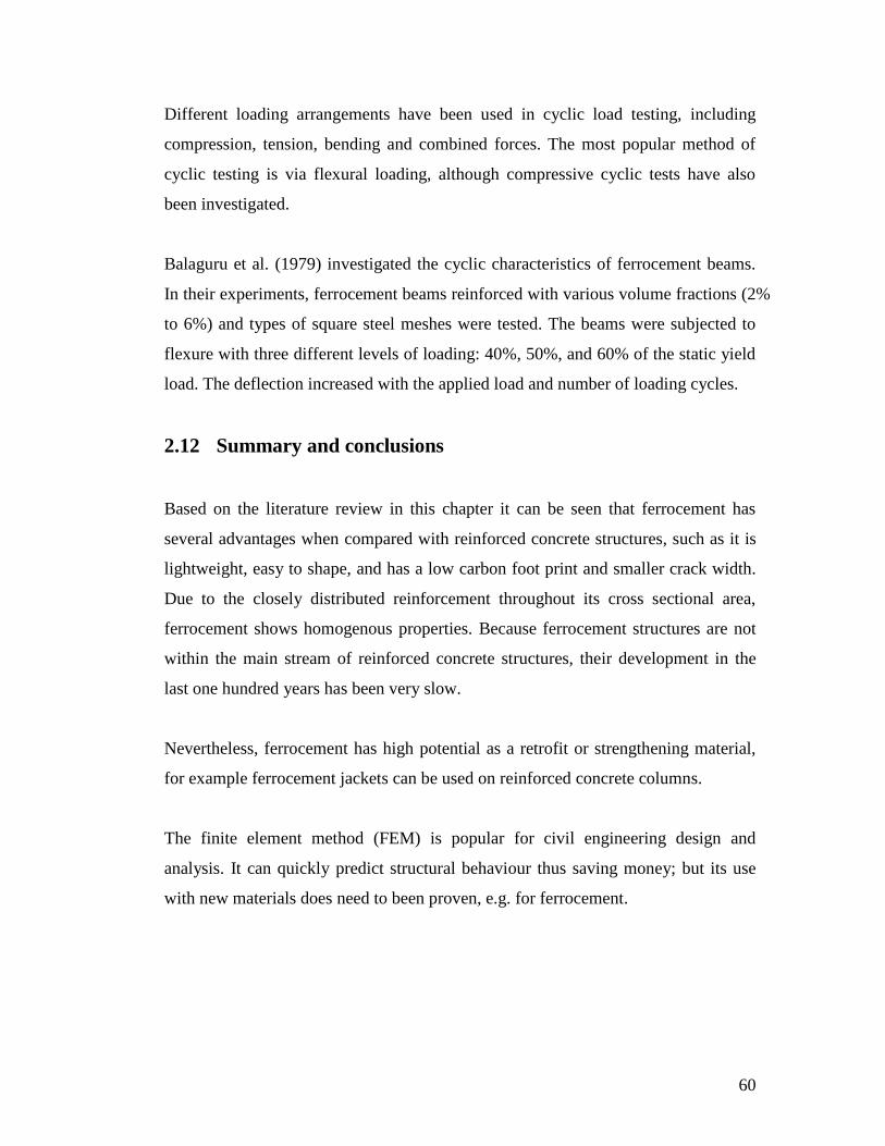
60

Different loading arrangements have been used in cyclic load testing, including

compression, tension, bending and combined forces. The most popular method of

cyclic testing is via flexural loading, although compressive cyclic tests have also

been investigated.

Balaguru et al. (1979) investigated the cyclic characteristics of ferrocement beams.

In their experiments, ferrocement beams reinforced with various volume fractions (2%

to 6%) and types of square steel meshes were tested. The beams were subjected to

flexure with three different levels of loading: 40%, 50%, and 60% of the static yield

load. The deflection increased with the applied load and number of loading cycles.

2.12 Summary and conclusions

Based on the literature review in this chapter it can be seen that ferrocement has

several advantages when compared with reinforced concrete structures, such as it is

lightweight, easy to shape, and has a low carbon foot print and smaller crack width.

Due to the closely distributed reinforcement throughout its cross sectional area,

ferrocement shows homogenous properties. Because ferrocement structures are not

within the main stream of reinforced concrete structures, their development in the

last one hundred years has been very slow.

Nevertheless, ferrocement has high potential as a retrofit or strengthening material,

for example ferrocement jackets can be used on reinforced concrete columns.

The finite element method (FEM) is popular for civil engineering design and

analysis. It can quickly predict structural behaviour thus saving money; but its use

with new materials does need to been proven, e.g. for ferrocement.

61

CHAPTER 3 Experimental tests

3.1 Introduction

This chapter presents details of the experimental tests reported in this thesis. These

include:

Material property tests: Five materials/elements were tested: concrete,

matrix, 12 mm ribbed steel bar, 3 mm general steel bar and welded mesh.

The results are used as input values for the Finite Element Model (FEM)

Casting the column specimens: Eight columns were cast and tested.

Five were tested using static loads and three using cyclic load

application. All the tests used displacement control.

The equipment setup: The specimens were tested as horizontal

cantilevers, with one end fixed, and the load applied to the other end.

Linear potentiometers (linpots) were distributed on the bottom surface of

each specimen.

3.2 Material property tests: concrete and matrix

3.2.1 Experiment preparation

The experimental programme included casting, curing and testing the specimens. In

general, the experiments were based on the concrete test code: BS EN 12350 (BSI,

2009) “Testing fresh concrete” and BS EN 12390 (BSI, 2010) “Testing hardened

concrete”.

62

The concrete and matrix both contain cement, sand, aggregates and water in

accordance with code BS EN 12350 (BSI, 2009). The details of the components are

given below:

Cement: The cement used was Ordinary Portland Cement (OPC), which

was stored under dry conditions, so that the cement used in the

experiments was fresh and free of lumps and other foreign matter.

Fine aggregates: Normal-weight natural river sand and uncrushed gravel

were used in the matrix. The maximum particle size was 2.36 mm,

passing through a No. 7 sieve.

Coarse aggregates: The coarse aggregate used was uncrushed gravel

with a maximum particle size of 10 mm.

Water: Clean and fresh potable tap water was used throughout, being free

of organic matter and acidic material.

Admixtures: Silica fume and superplasticiser were used to enhance the

strength of the matrix.

The mix ratios for concrete and the matrix were constant for all of the experimental

tests.

For the concrete: The proportions of the cement, water, fine and coarse aggregate

were: 484 kg/m3, 230 kg/m

3, 616 kg/m

3 and 1050 kg/m

3 respectively, which is based

on BS 8500 (BSI, 2006).

For the matrix: The cement and sand were mixed in the ratio of 1:2 by weight, and

water cement ratio was 0.4. The admixtures added were 10% of silica-fume by

weight of cement and 1.5% of superplasticiser (Paul and Pama, 1978).

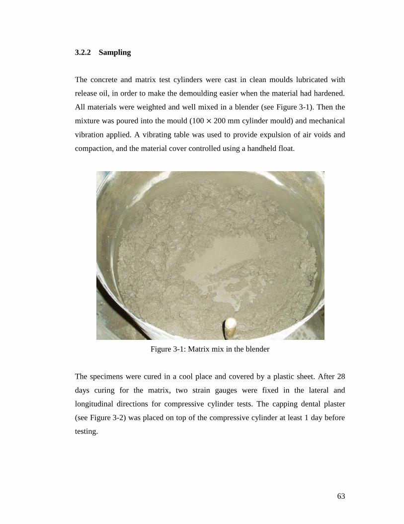
63

3.2.2 Sampling

The concrete and matrix test cylinders were cast in clean moulds lubricated with

release oil, in order to make the demoulding easier when the material had hardened.

All materials were weighted and well mixed in a blender (see Figure 3-1). Then the

mixture was poured into the mould (100 200 mm cylinder mould) and mechanical

vibration applied. A vibrating table was used to provide expulsion of air voids and

compaction, and the material cover controlled using a handheld float.

Figure 3-1: Matrix mix in the blender

The specimens were cured in a cool place and covered by a plastic sheet. After 28

days curing for the matrix, two strain gauges were fixed in the lateral and

longitudinal directions for compressive cylinder tests. The capping dental plaster

(see Figure 3-2) was placed on top of the compressive cylinder at least 1 day before

testing.

64

Figure 3-2: Horizontal and vertical strain gauges, and the dental plaster

3.2.3 Specimen tests

3.2.3.1 Compressive test:

The cylinders were centred on the lower platen of the testing machine. A constant

rate of 1 kN/sec loading was selected (BSI, 2010), the load and strain recorded. The

compressive strength is:

Eq 3-1

Where:


Maximum load at failure

Cross sectional area of the cylinder

65

The value of Young’s Modulus ( ), and Poisson's ratio ) were calculated from the

longitudinal and lateral stress-strain curves:

) Eq 3-2

Where:

The yield stress

The strain at yield stress

) Eq 3-3

Where:

The lateral strain at yield stress

3.2.3.2 Split test:

Based on BS EN 12390 (BSI, 2010), a constant loading rate of 0.05 kN/s was used

for the split test. The split test was used to determine the tensile properties of the

concrete and the matrix. Figure 3-3(a) is shown the steel jig and Figure 3-3(b) shows

a typical cylinder failure in the split test. Eq 3-4 gives the tensile stress formula.

Figure 3-3: The tensile test (a): jig with packing strips, (b): cylinder split test failure

(a)

(b)

66

)

Eq 3-4

Where:

Maximum loading at failure

D Diameter of cylinder

Length of cylinder

3.2.4 The test results

Typical stress-strain curves for concrete and the matrix under compression are

shown in Figures 3-4 and 3-5, and results present in Table 3-1. The compressive

strength of concrete reached 38 N/mm2, and compressive strength of matrix reached

62 N/mm2. The values of Young’s Modulus were 27500 N/mm

2 and 21000 N/mm

2

respectively. The result of split test for concrete was 3.74 N/mm2, for matrix is

reached 4.44 M/mm2.

Figure 3-4: Typical concrete cylinder compressive test of stress-strain curve

0

10

20

30

40

0 0.0005 0.001 0.0015 0.002 0.0025 0.003 0.0035

Str

ess

(MP

a)

Strain

Concrete test

67

Figure 3-5: Typical matrix cylinder compressive test of stress-strain curve

Table 3-1: The material properties of the concrete and the matrix

Material

Compression

strength

(N/mm2)

Young's

Modulus

(N/mm2)

Poisson's ratio

Tensile

stress

(N/mm2)

Concrete 38 27500 0.22 3.74

Matrix 62 21000 0.22 4.44

3.3 Reinforcing material tests

Three different types of reinforcing material were used for the reinforced concrete

and ferrocement specimens.

1) 12 mm diameter ribbed steel bar

2) 3 mm diameter general steel bar

3) Galvanised square welded steel mesh with 1.6 mm wire diameter,

12.6 mm mesh opening

0

10

20

30

40

50

60

70

0 0.0005 0.001 0.0015 0.002 0.0025 0.003 0.0035 0.004

Str

ess

(MP

a)

Strain

Matrix test

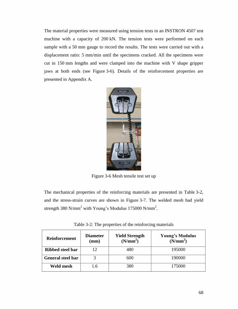
68

The material properties were measured using tension tests in an INSTRON 4507 test

machine with a capacity of 200 kN. The tension tests were performed on each

sample with a 50 mm gauge to record the results. The tests were carried out with a

displacement ratio: 5 mm/min until the specimens cracked. All the specimens were

cut in 150 mm lengths and were clamped into the machine with V shape gripper

jaws at both ends (see Figure 3-6). Details of the reinforcement properties are

presented in Appendix A.

Figure 3-6 Mesh tensile test set up

The mechanical properties of the reinforcing materials are presented in Table 3-2,

and the stress-strain curves are shown in Figure 3-7. The welded mesh had yield

strength 380 N/mm2 with Young’s Modulus 175000 N/mm

2.

Table 3-2: The properties of the reinforcing materials

Reinforcement Diameter

(mm)

Yield Strength

(N/mm2)

Young’s Modulus

(N/mm2)

Ribbed steel bar 12 480 195000

General steel bar 3 600 190000

Weld mesh 1.6 380 175000

69

Figure 3-7: Typical reinforcement properties from the experimental tests

3.4 Column Specimens

A sequence of 8 columns was proposed in order to investigate the effects of

reinforcement amount on the static and cyclic load behaviour. Table 3-3 below gives

the columns and their designation. Control columns of reinforced concrete were

provided and compared with ferrocement columns with four layers of mesh (which

provides a similar area of longitudinal steel) and two layers of mesh to investigate

the effect of steel content. In addition control columns which had been overlain with

two and three layers of mesh were used to investigate strengthening. The

relationships between the eight specimens are shown in Figure 3-8.

0

100

200

300

400

500

600

700

800

0 0.025 0.05 0.075 0.1 0.125 0.15 0.175

Str

ess

(MP

a)

Strain

1.6 mm Welded mesh

3 mm Stirrup

12 mm Steel bar

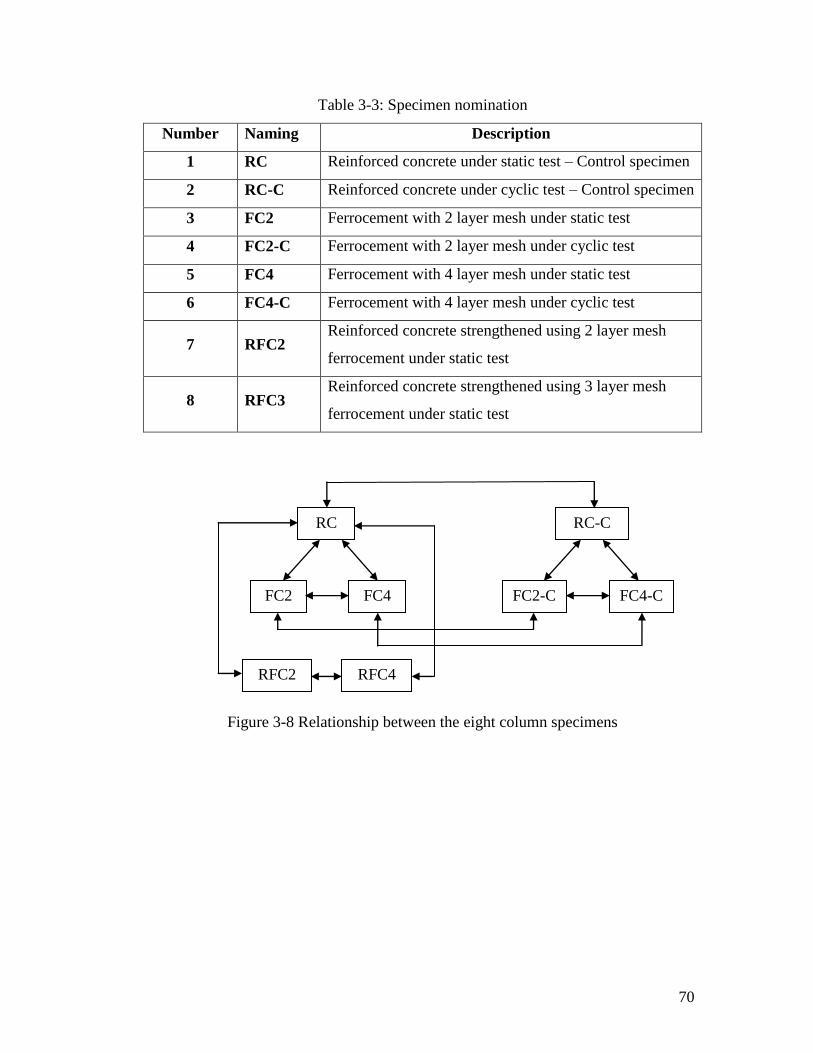
70

Table 3-3: Specimen nomination

Number Naming Description

1 RC Reinforced concrete under static test – Control specimen

2 RC-C Reinforced concrete under cyclic test – Control specimen

3 FC2 Ferrocement with 2 layer mesh under static test

4 FC2-C Ferrocement with 2 layer mesh under cyclic test

5 FC4 Ferrocement with 4 layer mesh under static test

6 FC4-C Ferrocement with 4 layer mesh under cyclic test

7 RFC2 Reinforced concrete strengthened using 2 layer mesh

ferrocement under static test

8 RFC3 Reinforced concrete strengthened using 3 layer mesh

ferrocement under static test

Figure 3-8 Relationship between the eight column specimens

RC RC-C

FC2 FC4 FC2-C FC4-C

RFC2 RFC4

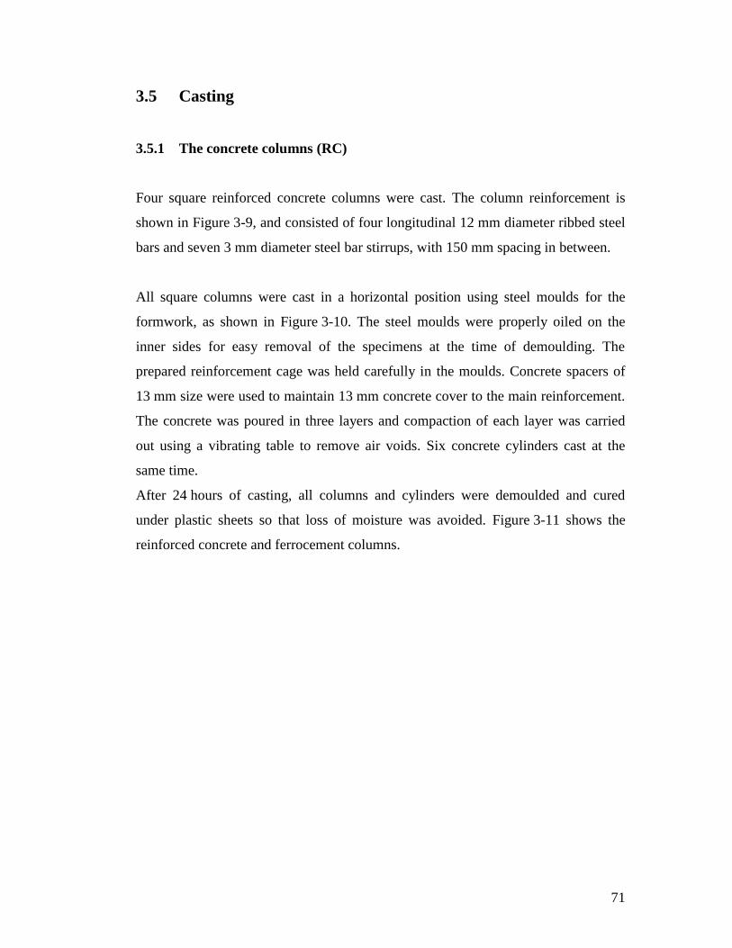
71

3.5 Casting

3.5.1 The concrete columns (RC)

Four square reinforced concrete columns were cast. The column reinforcement is

shown in Figure 3-9, and consisted of four longitudinal 12 mm diameter ribbed steel

bars and seven 3 mm diameter steel bar stirrups, with 150 mm spacing in between.

All square columns were cast in a horizontal position using steel moulds for the

formwork, as shown in Figure 3-10. The steel moulds were properly oiled on the

inner sides for easy removal of the specimens at the time of demoulding. The

prepared reinforcement cage was held carefully in the moulds. Concrete spacers of

13 mm size were used to maintain 13 mm concrete cover to the main reinforcement.

The concrete was poured in three layers and compaction of each layer was carried

out using a vibrating table to remove air voids. Six concrete cylinders cast at the

same time.

After 24 hours of casting, all columns and cylinders were demoulded and cured

under plastic sheets so that loss of moisture was avoided. Figure 3-11 shows the

reinforced concrete and ferrocement columns.

72

Figure 3-9: Reinforcement arrangement in the concrete column

150 mm

150 m

m

20 mm

4@12 mm diameter main longitudinal bars

3 mm link bars

60 m

m

1020 m

m

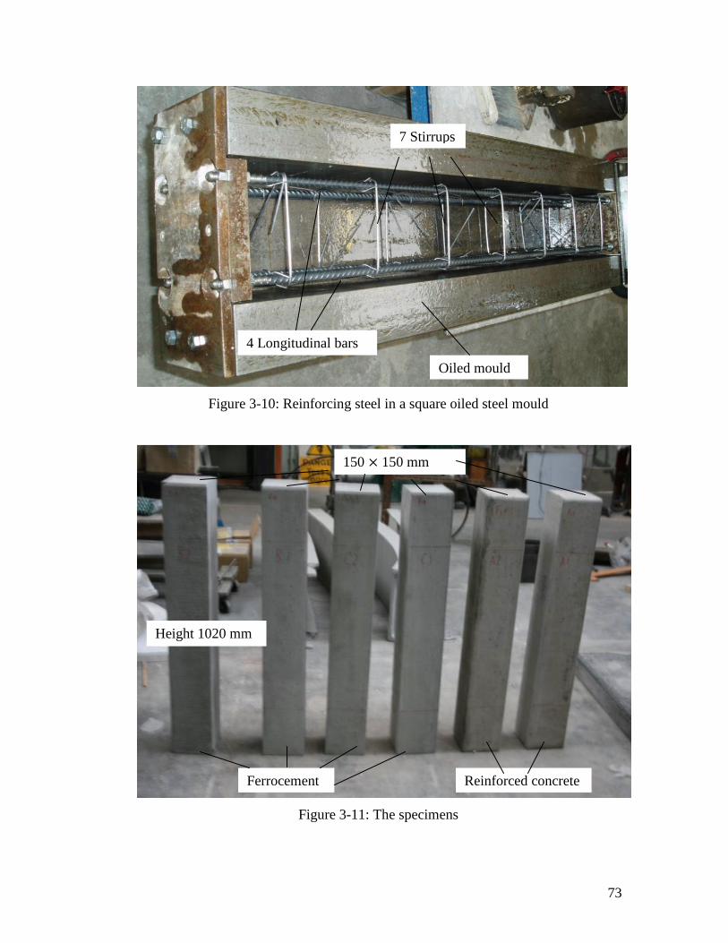
73

Figure 3-10: Reinforcing steel in a square oiled steel mould

Figure 3-11: The specimens

150 150 mm

Height 1020 mm

Ferrocement Reinforced concrete

7 Stirrups

Oiled mould

4 Longitudinal bars

74

3.5.2 The ferrocement columns (FC)

Four ferrocement columns were cast; two columns had two-layers of glazed welded

mesh, and two had four-layers of mesh. The skeleton of reinforcing mesh is box

section, which had 2 or 4 layers enclosed with plastic ties and a 3 mm matrix cover.

Figure 3-12 shows the patterns of the 2 layers and 4 layers mesh.

The method and mould used for casting the concrete columns was also used for the

ferrocement columns, as shown in Figure 3-13. More vibration sequences were

needed to ensure the matrix was evenly distributed through the whole specimen,

because the matrix does not easily pass through the layer meshes, especially for

four-layer meshes ferrocement. A wooden stop end was added to position the

column and to make demoulding easier. Again, the cylinders were cast at the same

time, and the columns and cylinders demould after 24 hours casting, then fully

covered with plastic sheet for curing.

Figure 3-12: The pattern of 2 and 4 layers mesh in the ferrocement columns

150 mm

150 m

m 2 layers mesh 4 layers mesh

3 mm cover 12.6 mm opening

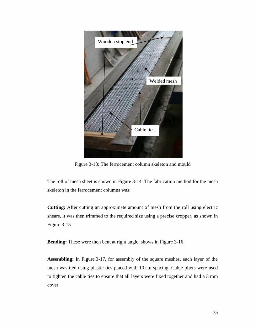
75

Figure 3-13: The ferrocement column skeleton and mould

The roll of mesh sheet is shown in Figure 3-14. The fabrication method for the mesh

skeleton in the ferrocement columns was:

Cutting: After cutting an approximate amount of mesh from the roll using electric

shears, it was then trimmed to the required size using a precise cropper, as shown in

Figure 3-15.

Bending: These were then bent at right angle, shows in Figure 3-16.

Assembling: In Figure 3-17, for assembly of the square meshes, each layer of the

mesh was tied using plastic ties placed with 10 cm spacing. Cable pliers were used

to tighten the cable ties to ensure that all layers were fixed together and had a 3 mm

cover.

Wooden stop end

Cable ties

Welded mesh

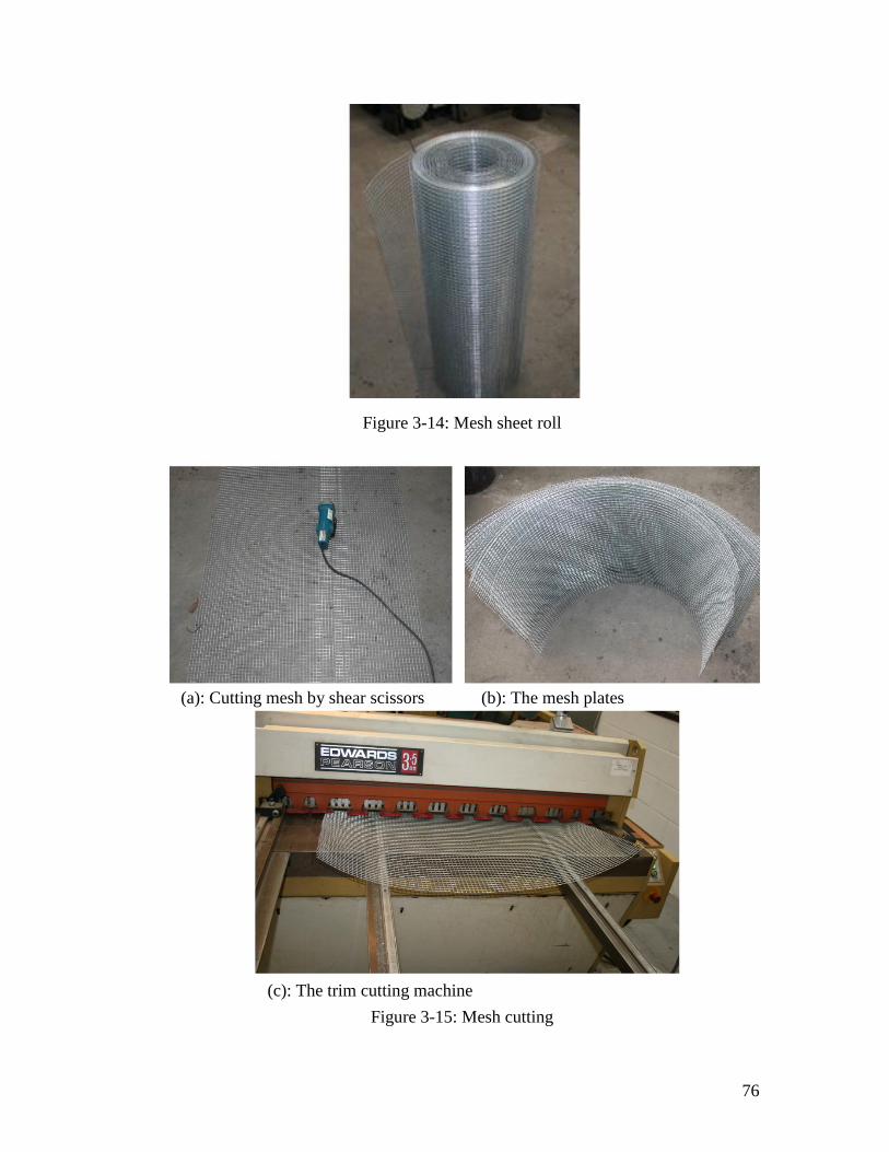
76

Figure 3-14: Mesh sheet roll

Figure 3-15: Mesh cutting

(a): Cutting mesh by shear scissors (b): The mesh plates

(c): The trim cutting machine

77

Figure 3-16: Mesh bending

(a): The bending machine

(b): The square shape meshes

78

Figure 3-17: The assembly of mesh layers with plastic ties

3.5.3 Reinforced concrete column strengthened using ferrocement jacket

(RFC)

After 28 days of the two reinforced concrete columns were strengthened using

ferrocement jacket, one with two-layers mesh, the other with three-layers.

Figure 3-18 shows the pattern of two and three-layers mesh around the reinforced

concrete.

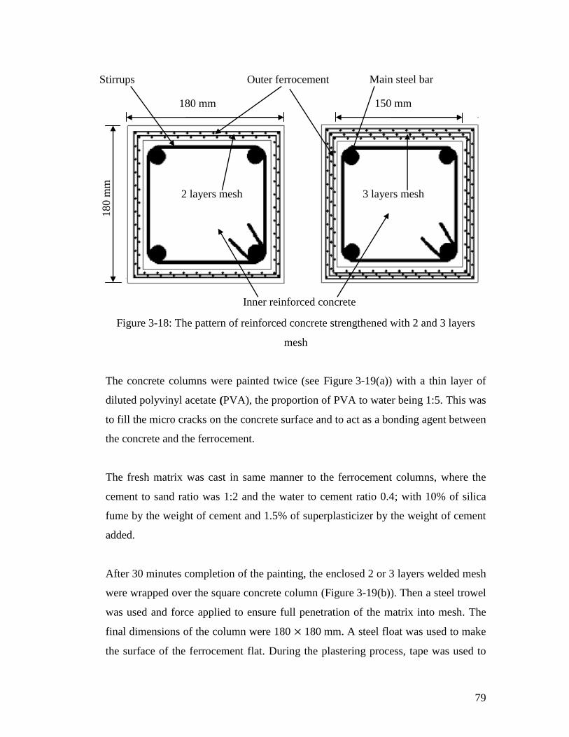
79

Figure 3-18: The pattern of reinforced concrete strengthened with 2 and 3 layers

mesh

The concrete columns were painted twice (see Figure 3-19(a)) with a thin layer of

diluted polyvinyl acetate (PVA), the proportion of PVA to water being 1:5. This was

to fill the micro cracks on the concrete surface and to act as a bonding agent between

the concrete and the ferrocement.

The fresh matrix was cast in same manner to the ferrocement columns, where the

cement to sand ratio was 1:2 and the water to cement ratio 0.4; with 10% of silica

fume by the weight of cement and 1.5% of superplasticizer by the weight of cement

added.

After 30 minutes completion of the painting, the enclosed 2 or 3 layers welded mesh

were wrapped over the square concrete column (Figure 3-19(b)). Then a steel trowel

was used and force applied to ensure full penetration of the matrix into mesh. The

final dimensions of the column were 180 180 mm. A steel float was used to make

the surface of the ferrocement flat. During the plastering process, tape was used to

2 layers mesh 3 layers mesh

Inner reinforced concrete

Outer ferrocement

180 mm 150 mm 180 m

m

Main steel bar Stirrups

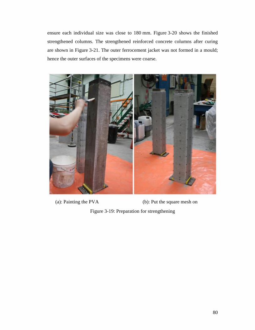
80

ensure each individual size was close to 180 mm. Figure 3-20 shows the finished

strengthened columns. The strengthened reinforced concrete columns after curing

are shown in Figure 3-21. The outer ferrocement jacket was not formed in a mould;

hence the outer surfaces of the specimens were coarse.

Figure 3-19: Preparation for strengthening

(a): Painting the PVA (b): Put the square mesh on

81

Figure 3-20: Casting the strengthened concrete column with ferrocement

Figure 3-21: Reinforced concrete columns strengthen with ferrocement jackets

82

3.6 The experimental rig

3.6.1 The methodology

The specimens were tested under a combination of axial load and bending.

Figure 3-22 shows a schematic plot of the experimental programme with the arrow

indicating the force P (axial load) and V (lateral load).

For safety, reliability and operability issues, all specimens were tested in a horizontal

cantilever position under bi-directional loading, as shown Figure 3-22(b). The static

load was applied in the pushing (downward) direction while the cyclic loading was

in both pushing and pulling directions. Reversed vertical cyclic loading represents

the seismic force, which was applied using a servo controlled hydraulic actuator to

the end of the columns. In the test schematic (Figure 3-22(b)), the left shaded area

was fixed end while the right shaded area is the loading area of the lateral force (V)

applied by the actuator. The setup of the column specimen is shown in Figure 3-23.

Figure 3-22: The column design layout, and test design layout as a cantilever

P

V V

P

Fixed end

Fixed end

(a): Normal column

(b): Test in horizontal cantilever position

P

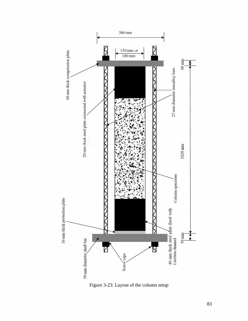
83

Figure 3-23: Layout of the column setup

84

Figure 3-23 shows the design layout for the test and provides various dimensions.

The axial load (P) was applied to the columns by two high strength calibrated

Macalloy bars (25 mm in diameter). The Macalloy bar at the fixed end was tied with

a 50 mm diameter shaft-bar and protection-plate. At the actuator end, the bars were

connected to a compression-plate. By tightening the nuts at the compression-plate,

the axial tensile forces were distributed evenly to the Macalloy bars at 100 kN using

a hydraulic jack, and then locked using the nuts (see detailed explanation in § 3.7).

The fixed end of column was secured using three (20 mm thick) stiff fixed-end

plates with two plates on top and one underneath. The lower steel plate sat on the

heavy primary beam of the testing frame (detail see Figure 3-31). Eight steel rods

were tied to the plates with high strength bolts to make sure that the end was fixed

(see Figure 3-24). Also, the other end of the column was connected to two similar

plates (20 mm thick), with one above and the other below and tightened by six high

strength steel rods.

The lateral load was applied by a 500 kN capacity hydraulic actuator with a pin

frame connector (see Figures 3-25 and 3-26). Four 10 mm diameter high strength

screws connected the pin joint and the loading area plate. The pin frame was used to

ensure the force applied was always perpendicular to the specimen’s top surface.

When the surface of the reinforced concrete column strengthened using ferrocement

jacket was not uniform, thick dental plaster was added to both the fixed end area and

the load-applied area, to ensure that the contact surface was flat (see Figure 3-27).

85

Figure 3-24: The design layout of the test setup (parts detail are shown in Table 3-4)

Table 3-4: Detail of dimension for each parts

Name of part Description

Fixed end plate 3@200 280 20 mm with 8@ 13 mm diameter holes

Loading area plate

2@200 280 20 mm both have 6@ 11 mm diameter

holes, and top plate has 4@ 11 mm diameter holes which

connect with actuator

Compression plate 2@ 200 280 20 mm with 2@ 26 mm diameter holes

Protection plate 1@150 150 10 mm for 150 150 mm specimens

1@180 180 10 mm for 180 180 mm specimens

Shaft bar 1@50 mm diameter with 500 mm length

Macalloy bar 2@25 mm diameter with 1500 mm length

High strength bolt 8@12 mm diameter with 400 mm length for support end

6@10 mm diameter with 300 mm length for loading area

Shaft bar

Protection plate

Specimen

Macalloy bar

Compression plate

Loading area plate

High strength bolts

Fixed end plate

Connect to actuator

86

Figure 3-25 A column setup on the equipment before the test

Figure 3-26 The pin joint between actuator and thick steel plate

Pin frame connector

Actuator

Hinge connector with actuator

Hinge connector with loading area plate Loading area plate

Hinge bar

Screws

Macalloy bar

Actuator

Specimen

s Shaft bar

Compression plate

Fixed end plate

Protection plate

High strength bolt

Gauge wire

Pin frame connector

Loading area plate

87

Figure 3-27: Dental plaster

3.6.2 The position of the linear potentiometers

Initially, eight linear potentiometers (linpots) were positioned beneath the specimen

in two lines, 150 mm apart, to measure the deflection of the specimen during the test

(see Figure 3-28(a)). It was proven that the specimen did not twist. After that a new

arrangement of linpots was used for the remaining specimens (see Figure 3-28(b)),

that one line of linpots at 75 mm spacing.

The selected naming for the linpots (Li) was F or B (Front or Back) and number (1-4

for initial arrangement, 1-7 for final arrangement) along the length between the

support and the free-end (for details see Figure 3-28). The Li-A is shown the

downward of actuator position.

For accuracy, all the linpots were fixed on a frame lying on the ground. Figure 3-29

shows the final arrangement of linpots beneath the specimen. Notice that the all

linpots were independent of the framework. The author made a simple aluminium

frame for the linpots, which laid under each specimen when tested. Figure 3-30

shows the two extra linpots at top of fixed-end area to measure the movement the

support.

(a): Fixed end area (b): Loading area

Dental plaster

88

Figure 3-28: Location of linpots under the specimen, (a): initial arrangement,

(b): final arrangement

Figure 3-29: Arrangement of linpots on the underside of the specimen

200 mm 150 mm 150 mm 150 mm 200 mm

140 mm 30 mm 100 mm

140 mm

200 mm 75 mm 75 mm 200 mm

15

0 m

m

Fixed-end area Actuator loading

area

a) Initial

arrangement

b) Finial

arrangement

. .. .

. .

. .

. . . .

. .

. .

. . 1020 mm

. .

. .

. .

. .

. .

. .

. .

. .

. .

15

0 m

m 75 mm

LiF1 LiF2 LiF3 LiF4

LiB1 LiB2 LiB3 LiB4 Li-A

Li1 Li2 Li3 Li4 Li5 Li6 Li7 Li-A

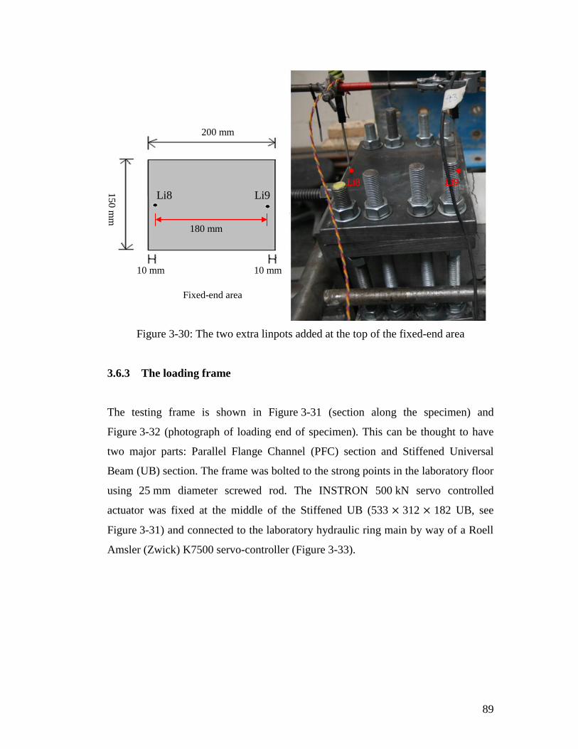
89

Figure 3-30: The two extra linpots added at the top of the fixed-end area

3.6.3 The loading frame

The testing frame is shown in Figure 3-31 (section along the specimen) and

Figure 3-32 (photograph of loading end of specimen). This can be thought to have

two major parts: Parallel Flange Channel (PFC) section and Stiffened Universal

Beam (UB) section. The frame was bolted to the strong points in the laboratory floor

using 25 mm diameter screwed rod. The INSTRON 500 kN servo controlled

actuator was fixed at the middle of the Stiffened UB (533 312 182 UB, see

Figure 3-31) and connected to the laboratory hydraulic ring main by way of a Roell

Amsler (Zwick) K7500 servo-controller (Figure 3-33).

Fixed-end area

10 mm 10 mm

200 mm

15

0 m

m

Li8 Li9

Li8 Li9

. Li8 Li9

.

180 mm

90

Figure 3-31: Loading frame layout

620 mm

300 mm

360 mm

1900 mm

Shaft bar

Macalloy bars

Column Specimen

Actuator

Fixed point with

foundation floor Steel plate welded

with base channel

500 mm

200 mm 1600 mm

Stiffened: 600 400 179

Crossed: 360 100 54 PFC

Column: 360 100 54 PFC

Stiffened: 533 312 182 UB

533 mm

406 mm

Stiffened: 406 178 85 UB

Base: 330 100 46 PFC

91

Figure 3-32: Loading frame

92

Figure 3-33: The controller for both static and cyclic tests

3.7 Specimen set up and load application

Care was taken when positioning the specimens for each test. Due to the weight of

the specimens the overhead crane was used during their installation and removal.

The procedure adopted was as follows:

Unclamp both ends of the completed specimen, carefully remove and clean the work

area. Lift the new specimen into position, holding horizontally, supported by the

crane. Clamp the fixed end and move the actuator so that the pinned end can be

clamped whilst the specimen is horizontal. Then remove the crane support and apply

the axial load as described below.

Prior to testing a support framework for the displacement gauges (linpots) was

placed beneath the specimen.

3.7.1 Axial load application

The axial force was applied to the columns through two high strength (25 mm

diameter) calibrated Macalloy bars. At the fixed-end of the specimen was a 50 mm

93

diameter shaft-bar and protection-plate (see Figure 3-25). At the loading end was a

compression-plate. An axial tensile force of 100 kN was applied to each Macalloy

bar (total axial force is 200 kN). The strain gauge fixed at the middle of each

Macalloy bar and the connection with the strain indicator box, as shown in

Figure 3-36. For safety and convenience a plywood bar (see Figure 3-34) was used

to support the extension bar and prevent the heavy compression-plate moving.

In order to apply the load an extension bar (connected using an extra coupler, see

Figure 3-34) is added to the main bar. A hollow support (see Figure 3-35) with

access to tighten the main nut was then placed over the extension bar and a hollow

bore jack over this. A small spreader was placed over the extension bar and a further

nut tightened. The jack was then extended until the bar indicated a load of 100 kN.

The main nut was then tightened and the jack released to put the axial force into to

the specimen. The operation was repeated on the second bar. The first bar was then

checked to ensure that there were no losses, and the force was topped up if necessary.

The jacking equipment and extension bar were then removed for the test.

Figure 3-34: Extension bar and coupler

Coupler Main nut

Extension bar Compression-plate

Plywood

94

Figure 3-35: The hydraulic jack connection with the end of the Macalloy bar with an

extra bar

Figure 3-36: The strain gauge fixed at the middle of each Macalloy bar and the

connection with the strain indicator box

3.7.2 Lateral load application

Two types of lateral loading were applied: Static and Cyclic. For both loads, the

actuator was controlled in its displacement mode. The static tests were carried out

first as their results provided the displacement for the cyclic load (detail shown

below).

(a)

(b)

Jack Hollow support

Nut

Spreader plate

Strain gauge wire

Main nut

95

The test sequence was RC, FC2, FC4, RFC2, RFC3, RC-C, FC2-C and FC4-C, As

described in Table 3-3.

Static loading test: The actuator was moved uniformly at 0.5 mm/s, which

guaranteed sufficient data, with recording scans twice every second.

Cyclic loading test: The amplitude (A) for each test was 60% of the ultimate

achieved in the static test, as shown in Eq 3-5.

Eq 3-5

Where:

Amplitude of test applied

The peak load of the specimen under static loading

The test of cyclic load, started with a slow single cycle (0.5 mm/s) to record

displacement throughout. Then, the actuator applied high movement speed at 1 Hz.

As the data recorder was not able to capture sufficient data at the faster speed it was

decided to carry out a low speed cycle at the predetermined intervals of 100, 200,

400 and 600 cycles. Finally, the actuator applied a static load to test the specimen to

failure.

3.8 Summary

In this chapter the tests to establish material properties were presented, together with

the fabrication method, the equipment design and the testing of the specimens. The

following points are emphasized:

a) Material property tests have been conducted, including concrete, matrix,

12 mm diameter steel bar (longitudinal ribbed bar in RC), 3 mm

diameter bar (transverse bar in RC) and welded mesh. The concrete and

96

matrix properties were tested, that includes compression and split tests,

using 100 200 mm cylinders.

b) Eight columns were cast: 2 reinforced concrete columns, 4 ferrocement

columns and 2 strengthening reinforced concrete using ferrocement

jacket columns.

c) The fabrication of the skeleton ferrocement includes cutting, bending

and assembling from a roll of the mesh.

d) For safety, reliability and operability issues, all specimens were tested in

a horizontal cantilever position. The two Macalloy bars applied constant

axial load and the actuator applied lateral load.

e) The connector between actuator and loading area plate was a pin frame.

f) The linpots were located beneath the specimens.

g) The cyclic load test used a constant frequency (1 Hz), with constant

amplitude (A). The amplitude was 60% of the ultimate achieved in the

static test.

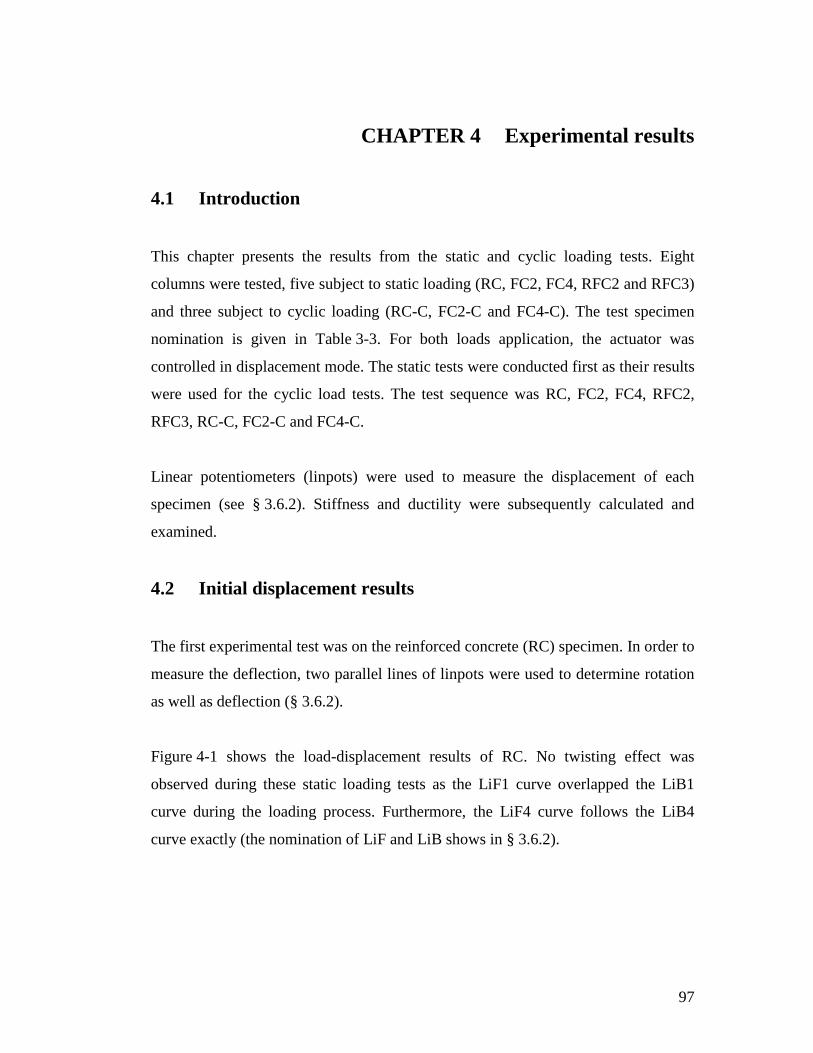
97

CHAPTER 4 Experimental results

4.1 Introduction

This chapter presents the results from the static and cyclic loading tests. Eight

columns were tested, five subject to static loading (RC, FC2, FC4, RFC2 and RFC3)

and three subject to cyclic loading (RC-C, FC2-C and FC4-C). The test specimen

nomination is given in Table 3-3. For both loads application, the actuator was

controlled in displacement mode. The static tests were conducted first as their results

were used for the cyclic load tests. The test sequence was RC, FC2, FC4, RFC2,

RFC3, RC-C, FC2-C and FC4-C.

Linear potentiometers (linpots) were used to measure the displacement of each

specimen (see § 3.6.2). Stiffness and ductility were subsequently calculated and

examined.

4.2 Initial displacement results

The first experimental test was on the reinforced concrete (RC) specimen. In order to

measure the deflection, two parallel lines of linpots were used to determine rotation

as well as deflection (§ 3.6.2).

Figure 4-1 shows the load-displacement results of RC. No twisting effect was

observed during these static loading tests as the LiF1 curve overlapped the LiB1

curve during the loading process. Furthermore, the LiF4 curve follows the LiB4

curve exactly (the nomination of LiF and LiB shows in § 3.6.2).

98

Figure 4-1: Load-displacement relationships for LiF1, LiB1, LiF4 and LiB4 (RC)

After the first column (RC) test, a new arrangement of linpots was used for the

remaining column specimens, which is a single line with 75 mm spacing, as shown

in Figure 3-28.

4.3 The displacement at the top of the fixed-end plate

During the second test (FC2), the author observed that the fixed-end plate (see

Figure 3-25) had a slight movement. Therefore, two extra linpots were added at the

fixed-end plate and an additional test was performed (FC4). The two extra linpots

(Li8 and Li9) were located at the positions shown in Figure 3-30, where Li8 was

located 10 mm from one edge at the top surface of the fixed-end plate and Li9 was

located 10 mm from the other edge.

99

Figure 4-2: Load-displacement relationships for Li8, Li9 and best-fit linear curves

A reasonably linear relationship was observed between lateral load and displacement.

Li8 had an upward movement with increasing load and a Li9 had a downward

movement. When FC4 reached 34.7 kN (the maximum load), Li8 had 1.3 mm

displacement, and Li9 had 1.1 mm displacement. After the peak load, both linpots

moved in the reverse direction in a linear manner.

Assumptions of the experimental test shown in Figure 4-3, which the 8 steel bars at

support end (see Figure 3-25) assumed connected with 2 linear springs. The forces

of the springs are F1 and F2. The top of support end assumed rigid body.

y = -27.4 x y = 30.5 x

0

5

10

15

20

25

30

35

40

45

-1.5 -1 -0.5 0 0.5 1 1.5

La

tera

l lo

ad

(k

N)

Displacement (mm)

Li8

Li9

Linear (Li8)

Linear (Li9)

100

Figure 4-3: Simplified diagram of the specimen at the support end

Where:

The lateral load applied by the actuator

Assumed forces balancing the lateral forces: position at the

edge of the concrete, position at 200 mm from the edge

The displacements at the edges

The distances from point and to point O. Point O has zero

displacement when lateral load applied

101

The stiffness of these two points can be calculated considering moment equilibrium

as:

Eq 4-1

Where:

Length from point O to actuator load position

The values of in Eq 4-1 are:

Then, value of L is 720 + 92.5 = 812.5 mm

By substituting the values of and into Eq 4-1 yields:

The load equilibrium is:

Then

Hence, the stiffness for each edge of the fixed-end plate is:

)

)

102

4.4 Reinforced concrete column under static load

Specimen RC had 4 longitudinal bars with 7 stirrups and the load-displacement

curves at various positions are shown in Figure 4-4. At the position under the

actuator (Li-A), the displacement showed linearity until the lateral load reached

approximately 30 kN, with a deflection of 16.5 mm. When the maximum load

capacity was reached (35.7 kN), the measured displacement was 23.9 mm. After the

peak load, the load reduced.

Observation of RC: The actuator applied force downward on the loading-plate with

a speed 0.5 mm/s. Initially, as the displacement increased, the value of lateral load

increased. The first crack was observed on the top surface near the fixed end, when

the actuator had moved 12 mm and the lateral load was approximately 23 kN. Then

more cracks were observed. As the actuator deflection increased, the cracks

penetrated from the top surface through to the underside. At an actuator

displacement of 23.9 mm, the lateral load reached its maximum, then the load

dropped the cracks continued to expand and concrete fragments started to drop from

the underside of the specimen at its fixed-end. The column after testing is shown in

Appendix C.

Figure 4-5 shows the displacement for each linpot at four different lateral loads

together with support rotation effect. The four loads selected, expressed as a multiple

of the peak load, were 0.33, 0.66, 1.00 and 0.85 post peak load. The components of

displacement at Li-A are shown in Figure 4-6, including total displacement and the

two major contributing factors, which are the support rotation effect and the

bending-shear effect.

103

Figure 4-4: Load-displacement curves at different positions (Initial column, RC)

Table 4-1 presents the support rotation effect and bending-shear effect displacement

percentage at different loads (33%, 66%, 100% and 85% post peak load).

At 33% peak load (11.9 kN), the support rotation effect provides 67% of the

displacement (3.5 mm), which is nearly twice the bending-shear effect. At 66% peak

load, the support rotation effect reduced to 57%. At approximately 90% peak load

(32.3 kN), the rotation and bending-shear effect were equal. The rotation effect

provides 44% at peak load (35.7 kN), after that the bending-shear effect was

dominant. At the 85% post peak load (30.3 kN), the percentage of the bending-shear

effect on the overall displacement rose to 76%

0

5

10

15

20

25

30

35

40

0 5 10 15 20 25 30 35 40

La

tera

l lo

ad

(k

N)

Displacement (mm)

RC: LiF1/LiB1

RC: LiF2/LiB2

RC: LiF3/LiB3

RC: LiF4/LiB4

RC: Li-A

104

Figure 4-5: Displacement for each linpot at different loads (Initial column, RC)


bending-shear effect at Li-A (Initial column, RC)

-5

0

5

10

15

20

25

30

35

40

0 200 400 600 800 1000

Dis

pla

cem

ent

(mm

)

Position (mm)

0.33 peak load support rotation


Peak load support rotation

0.85 post peak load support rotation

0.33 peak Load

0.66 peak load

Peak load

Failure

0%

10%

20%

30%

40%

50%

60%

70%

80%

90%

100%

0 5 10 15 20 25 30 35 40

La

tera

l lo

ad

per

cen

tag

e

Displacement (mm)

Total displacement

Support rotation effect

Bending and shear effect

0.33 peak load

0.66 peak load

0 85 post peak load

Peak load

105

Table 4-1: Results of the support rotation effect and the bending-shear effect (RC)

Specimen

Lateral load applied Total

disp.

(mm)

Support rotation

effect

Bending-shear

effect

Load (kN) Percent

(%)

Absolute

value

(mm)

Percent

(%)

Absolute

value

(mm)

Percent

(%)

RC

11.9 33% 5.2 3.5 67% 1.7 33%

23.8 67% 12.2 7.0 57% 5.2 43%

32.3 90% 18.8 9.5 50% 9.3 50%

35.7 100% 23.9 10.5 44% 13.4 56%

30.3 85% 36.2 8.9 24% 27.3 76%

Checking the result at 33% peak load for the RC specimen (5.2 mm for test, 3.5 mm

for rotation effect and 1.7 mm for bending-shear effect), with the load displacement

in the linear elastic stage. Using Eq 4-2, assume the specimen was a cantilever.

)

Eq 4-2

Where:

Cantilever deformation one the underside of point Li-A

Length of the cantilever

Lateral load

Young's Modulus of composite

Second moment of area

Poisson's ratio

h Width of column

The result of calculation of at 33% peak load is 1.6 mm (detail provided in

Appendix D), which is close to the bending-shear effect displacement (1.7 mm)

106

4.5 Ferrocement column under static load

FC2 and FC4 columns had an inner skeleton which was comprised of a box of

welded mesh with 3 mm cover on all sides. Figure 4-7 shows the test results at Li-A

(the full set of results are given in Appendix E), the load-displacement curve for

both specimens are similar; however, the maximum load capacity and deflection

were different.

Observation of FC2 and FC4: Initially, as the actuator deflection increased, the

value of lateral load rose. The first crack was observed at the top surface near the

fixed end at lateral loads of 16 kN for FC2, and 20 kN for FC4. After that, the first

crack grew and more cracks were observed. The observed crack width on FC2 was

greater than that on FC4. The cracks of both specimens penetrated from the top

surface to bottom surface, and could be observed on the surface at the front and back.

After the peak load (29 kN for FC2 and 34.7 kN for FC4), the load dropped and the

cracks continued to expand. Under the fixed-ends concrete fragments started to drop

from the specimens.

Both FC2 and FC4 had the same stiffness at the start of the test. FC2 reach a peak

load of 29 kN at 20.9 mm displacement, and FC4 reached a peak load 34.7 kN at

23.5 mm displacement. The 20% higher load capacity of FC4 is due to its higher

reinforcement content.

After the specimens had reached their peak loads, the load dropped. This drop is

significant for FC2 (see Figure 4-7); the bond slip occurred at the peak load with the

outer layer of mesh yielding. However as FC4 had a denser mesh (higher amount),

the bond slip effect was less. After that, in both specimens, the welded mesh carries

the load.

107

Figure 4-7: Load-displacement curves at Li-A (FC2 and FC4)

Figures 4-8 and 4-9 show load-displacement curves for the support rotation effect

and the bending-shear effect for FC2 and FC4 at Li-A, including the total

displacement. The support rotation effect and bending-shear effect displacement for

FC2 and FC4 at different load levels related to peak load (0.33, 0.66, 1.00 and 0.85

post peak load) are presented in Table 4-2.

With increasing lateral load, the percentage contributions of the support rotation

effect were reduced. At 33% peak load, the support rotation effect for both

specimens was significant, i.e. providing 65% of the displacement for FC2 and 69%

for FC4. The lateral loads, for FC2 was 9.26 kN, which is 10% lower than that for

FC4 (11.2 kN).

At 66% peak load, the rotation effect for FC2 had approximately the same

percentage (64%) as at 33% peak load, but for FC4, the rotation effect was less

important, reducing to 60%. The value of lateral load for each specimen was

18.6 kN for FC2, 23.1 kN for FC4.

0

5

10

15

20

25

30

35

40

0 5 10 15 20 25 30 35 40 45

La

tera

l lo

ad

(k

N)

Displacement (mm)

FC2: Li-A

FC4: Li-A

108

At approximately the same percentage of lateral load for both specimens (90% for

FC2, 91% for FC4), the bending-shear effect was equal to the support rotation effect.

At the peak load, the bending-shear effect for both specimens has a greater effect

than the rotation effect (40% for FC2 and 43% for FC4).

At 85% post peak load, the support rotation effect reduced to 28% for FC2 and 21%

for FC4.


bending-shear effect at Li-A (FC2)

0%

10%

20%

30%

40%

50%

60%

70%

80%

90%

100%

0 5 10 15 20 25 30 35 40 45

La

tera

l lo

ad

per

cen

tag

e

Displacement (mm)

Total displacement



0.33 peak load

0.66 peak load

0 85 post peak load

Peak load

109


bending-shear effect at Li-A (FC4)

Table 4-2: Results of the support rotation effect and the bending-shear effect (FC2

and FC4)

Specimen


disp.

(mm)

Support rotation

effect

Bending-shear effect

(mm)

Load (kN) Percent

(%)

Absolute

value

(mm)

Percent

(%)

Absolute

value

(mm)

Percent

(%)

FC2

9.7 33% 4.4 2.7 65% 1.6 35%

19.3 67% 8.5 5.4 64% 3.1 36%

26.1 90% 15.1 7.6 50% 7.5 50%

29.0 100% 20.9 8.3 40% 12.2 60%

24.7 85% 24.9 7.0 28% 17.9 72%

FC4

11.6 33% 4.8 3.3 69% 1.5 31%

23.1 67% 11.2 6.7 60% 4.5 40%

31.2 91% 18.2 9.1 50% 9.1 50%

34.7 100% 23.5 10 43% 13.5 57%

29.5 85% 40.8 8.5 21% 32.3 79%

0%

10%

20%

30%

40%

50%

60%

70%

80%

90%

100%

0 5 10 15 20 25 30 35 40 45

La

tera

l lo

ad

per

cen

tag

e

Displacement (mm)

Total displcaement



0.33 peak load

0.66 peak load

0 85 post peak load

Peak load

110

Checking the deformation result at 33% peak load for FC2 and FC4 using Eq 4-2.

For FC2, the result of is 1.79 mm and the bending-shear effect is 1.6 mm which

shows a 11% difference. For FC4, the result of is 1.93 mm and the bending-shear

effect is 1.5 mm which shows a 28% difference. This may be because in the

simplified sections in the hand calculations, the meshes are merged to form one layer

and are uniformly distributed in section. Details of the calculations are given in

Appendix D.

4.6 Reinforced concrete column strengthened using ferrocement

jacket under static load

RFC2 and RFC3 were reinforced concrete columns strengthened using ferrocement

jackets and were tested under static loading. The column cross-sections were

180 180 mm, the ferrocement was the same as for FC2 and FC4, with a cover of

3 mm. The test results for RFC2 and RFC3 are shown in Figure 4-10, and the

behaviour of these two columns was similar. Both columns show a significant

increase in load capacity at failure in comparison with RC.

The initial stiffness for both columns was less than RC. This might be due to the

possibility that the dental plaster did not provide a perfect contact (see Figure 3-27).

The dental plaster was to ensure the specimen support and loading areas were

uniform and horizontal. The ultimate load of RC without strengthening is 35.7 kN.

The columns strengthened using two-layers and three-layers of mesh achieved

50.9 kN and 57.7 kN respectively, representing nearly 46% and 66% extra capacities.

The outer ferrocement jacket played a confinement role, which provides a significant

increase in the load capacity. As the ductility of the welded mesh is high, it produces

a smoother descent stage in the load-displacement curve.

111

Figure 4-10: Load-displacement curves for the RC and strengthened RC columns

under static load at Li-A

Observation of RFC2 and RFC3: The first crack was observed at the top surface

near the fixed end, at a lateral load of around 30 kN for RFC2, and 33 kN for RFC3.

The observed crack widths for RFC2 and RFC3 were similar, and were small cracks

distributed on the top surface. After the peak load (RFC2 reached 50.9 kN and RFC3

reached 57.7 kN), the load dropped.

The support rotation effect and bending-shear effect on displacement of RFC2 and

RFC3 at different loads (0.33, 0.66, 1.00 and 0.85 post peak load) are presented in

Figures 4-11 and 4-12, the results are presented in Table 4-3. The displacement of

RFC2 at peak load was 33.6 mm and at 0.85 post peak load was 62 mm. RFC3 also

had a significant displacement difference between peak load and 85% post peak load.

At 33% peak load, the support rotation effect for both specimens was significant, 63%

for RFC2, 64% for RFC3. The lateral load for RFC2 was 17 kN and RFC3 was

19.2 kN.

0

10

20

30

40

50

60

0 10 20 30 40 50 60 70 80

La

tera

l lo

ad

(k

N)

Displacement (mm)

RC Test

RFC2 Test

RFC3 Test

112

At 66% peak load, the rotation effect for RFC2 was 56%, and for RFC3 was 58%.

The value of lateral load for each specimen was, 33.9 kN for RFC2 and 38.5 kN for

RFC3.

At approximately similar percentages of lateral load (91% for RFC2, 89% for RFC3)

for both specimens, the bending-shear effect equalled the support rotation effect.

At peak load, the bending-shear effect for both specimens had a greater effect than

the rotation effect (RFC2 had 45% and RFC3 had 44%).

At 85% post peak load, the bending-shear effect is significantly more important for

both specimens, being 79% for both specimens.


effect at Li-A (RFC2)

0%

10%

20%

30%

40%

50%

60%

70%

80%

90%

100%

0 10 20 30 40 50 60 70 80

La

tera

l lo

ad

per

cen

tag

e

Displacement (mm)

Total displacement



0.33 peak load

0.66 peak load

0 85 post peak load

Peak load

113


effect at Li-A (RFC3)

Table 4-3: Results of support rotation effect and bending-shear effect (RFC2 and

RFC3)

Specimen


disp.

(mm)

Support rotation

effect

Bending-shear effect

(mm)

Load (kN) Percent

(%)

Absolute

value

(mm)

Percent

(%)

Absolute

value

(mm)

Percent

(%)

RFC2

17.0 33% 8.0 5.1 63% 2.9 37%

33.9 67% 18.1 10.1 56% 8.0 44%

46.3 91% 27.6 13.8 50% 13.8 50%

50.9 100% 33.6 15.2 45% 18.4 55%

43.3 85% 62.0 12.9 21% 49.1 79%

RFC3

19.2 33% 9.1 5.7 64% 3.3 36%

38.5 67% 19.7 11.5 58% 8.2 42%

51.4 89% 30.8 15.3 50% 15.5 50%

57.7 100% 39.2 17.2 44% 22.0 56%

49.0 85% 70.8 14.6 21% 56.2 79%

0%

10%

20%

30%

40%

50%

60%

70%

80%

90%

100%

0 10 20 30 40 50 60 70 80

La

tera

l lo

ad

per

cen

tag

e

Displacement (mm)

Total displacement



0.33 peak load

0.66 peak load

0 85 post peak load

Peak load

114

Checking the deformation result at 33% peak load for RFC2 and RFC3 using Eq 4-2.

For RFC2, is 1.26 mm, and the bending-shear effect is 2.9 mm. For RFC3, is

1.43 mm, and the bending-shear effect is 3.3 mm. There are large differences for

these two columns, so the author calculated new second moment area (I) values

ignoring the tensile strength of the matrix and concrete. The value of is then

2.1 mm for RFC2 and 2.19 mm for RFC3. However, the results are still not good.

The reasons for this may be: the restrain cracks inside the concrete or matrix, the

imperfect bond between mesh and matrix, the non-uniform section, or the matrix had

not perfectly penetrated through the meshes.

4.7 Cyclic loading tests

Three specimens were tested under cyclic loading, RC-C, FC2-C and FC4-C.The

three tests followed the same procedure. Before the tests, the amplitude (A) was

found for each specimen, the amplitude was 60% of the peak value achieved in the

static test as shown in Eq 3-5. The amplitudes for RC, FC2-C and FC4-C were

14.5 mm, 12.5 mm and 14.0 mm.

4.7.1 Load reduction

The experimental test results are shown in Figures 4-13, 4-14 and 4-15. The positive

load represents the downward force applied by the actuator. For each specimen, the

amplitude was kept constant, so during the cyclic tests the loads showed a clear

decreasing trend. The results are presented in Figure 4-16; more detail is given in

Appendix E.

During the first cycle, RC-C reached a maximum load (26.6 kN at 14.5 mm), which

is higher than that for the another two specimens. The maximum load for FC2-C was

22.2 kN at 12.5 mm and for FC4-C was 25 kN at 14 mm.

115

After 100 cycles, the maximum load of RC-C reduced to 24.8 kN, which is 7%

lower than that for the first cycle. FC2-C was 10% lower (20 kN) and FC4-C was 7%

lower (23.2 kN).

After 200 cycles, RC-C reached 23.5 kN, which is 12% lower than that for the first

cycle, and after 400 cycles, the load further reduced (22.5 kN, 16% lower than the

first cycle), then after 600 cycles, the load reduced to 20.9 kN (21% lower than the

first cycle). FC2-C and FC4-C showed a similar trend to RC-C, where with an

increasing number of cycles, the maximum load dropped.

However, FC4-C was more stable than either FC2-C or RC-C, in that after 600

cycles, the load reduced by only 11% (see Figure 4-16). Here the dense welded mesh

acted as a confinement during the cyclic test and the crack width was much smaller

than that for RC-C. FC2-C also had a dense mesh as confinement, but it had less

reinforcement than FC4-C.

After 600 cycles, RC-C and FC2-C were pushed to failure, but for FC4-C, the load

just reduced by 11% (22.2 kN). Therefore, the author decided to increase the cyclic

load to 1000. The load reduced to 16.8 kN, 33% lower than the first cycle.

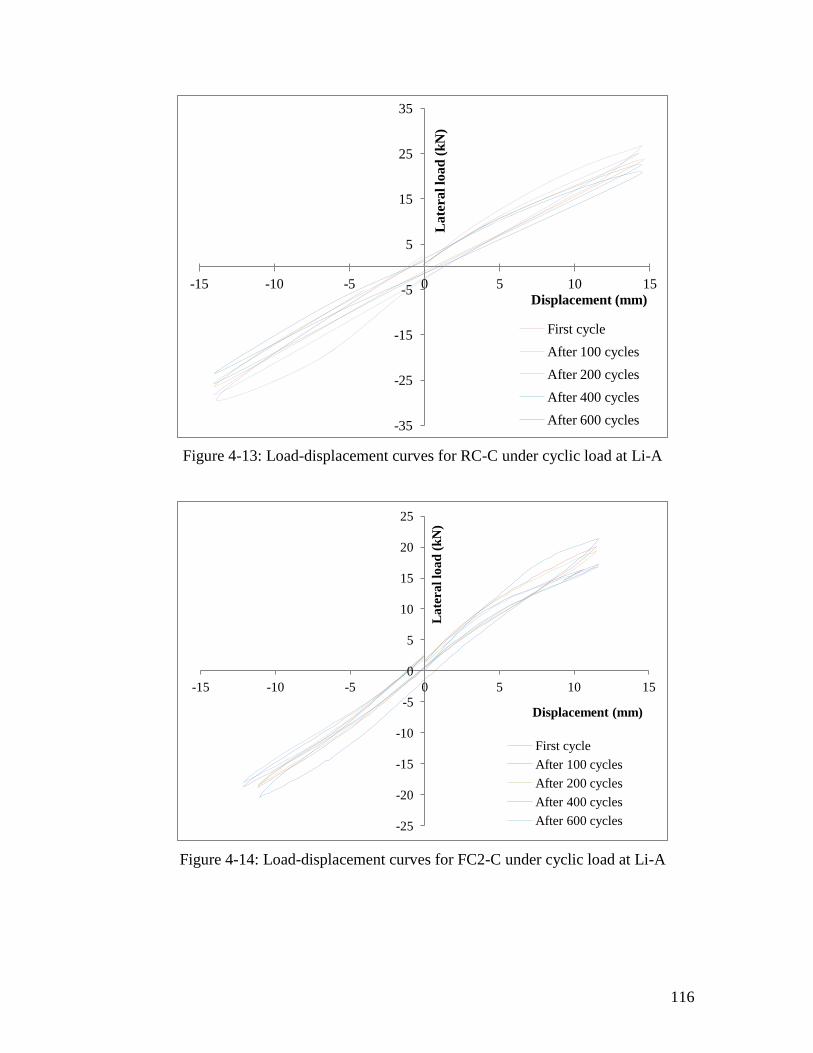
116

Figure 4-13: Load-displacement curves for RC-C under cyclic load at Li-A

Figure 4-14: Load-displacement curves for FC2-C under cyclic load at Li-A

-35

-25

-15

-5

5

15

25

35

-15 -10 -5 0 5 10 15

La

tera

l lo

ad

(k

N)

Displacement (mm)

First cycle

After 100 cycles

After 200 cycles

After 400 cycles

After 600 cycles

-25

-20

-15

-10

-5

0

5

10

15

20

25

-15 -10 -5 0 5 10 15

La

tera

l lo

ad

(k

N)

Displacement (mm)

First cycle

After 100 cycles

After 200 cycles

After 400 cycles

After 600 cycles

117

Figure 4-15: Load-displacement curves for FC4-C under cyclic load at Li-A

Figure 4-16: Load degradation against number of cycles (for details see Appendix E)

-40

-30

-20

-10

0

10

20

30

-20 -15 -10 -5 0 5 10 15 20

La

tera

l lo

ad

(k

N)

Displacement (mm)

First cycle

After 100 cycles

After 200 cycles

After 400 cycles

After 600 cycles

After 1000 cycles

60%

65%

70%

75%

80%

85%

90%

95%

100%

0 100 200 300 400 500 600 700 800 900 1000

Lo

ad

pre

cen

tag

e

Number of cycles

Load decrement (RC-C)

Load decrement (FC2-C)

Load decrement (FC4-C)

118

4.7.2 Stiffness degradation

The stiffness of column under cyclic load is degraded during number of cycles increase,

it calculated as initial slope of curve lateral load against displacement. The stiffness

degradation results are shown in Figure 4-17 and presented in Table 4-4. These three

specimens have similar values of stiffness for the first cycle (RC-C had 2.5 kN/mm,

FC2-C had 2.59 kN/mm and FC4 had 2.53 kN/mm).

After 100 cycles, the stiffness of RC-C dropped to 2.0 kN/mm, which is 20% lower

than the initial value (first cycle), FC2-C and FC4-C were 8% and 9% lower. The

reason for this is that the dense weld mesh is providing confinement, and it has

stopped the crack width from increasing. That is why it is said that the ferrocement

mesh structures have a huge potential for use in seismic zones.

After 200 cycles, the stiffness of RC-C was 1.95 kN/mm, which is 22% lower than

the initial stiffness. Then after 400 cycles and 600 cycles, the stiffness of RC-C

reduced to 1.84 kN/mm and 1.77 kN/mm. For FC2-C and FC4-C, the stiffness

reduced with increasing number of cycles, between 200 and 400 cycles, the stiffness

of FC2-C dropped much quicker than FC4-C. After 200 cycles, both specimens had

the same stiffness degradation (89% of initial stiffness), but after 400 cycles, the

stiffness of FC2-C had reduced to 1.99 kN/mm (23% lower than the initial value),

and FC4-C had reduced to 2.07 kN/mm (18% lower than the initial value).

After 600 cycles, the stiffness degradations for RC-C and FC2-C were similar, 71%

for RC-C and FC2-C for 72%, but for FC4-C the stiffness degradation was 79%.

The stiffness of FC4-C after 1000 cycles was 60%.

119

Figure 4-17: Stiffness degradation during number of cycles (for detail see Appendix

E)

Table 4-4: Stiffness and degradation of RC-C, FC2-C and FC4-C

No. of

cycles

RC-C FC2-C FC4-C

Stiffness

(kN/mm)

Stiffness

degradation

Stiffness

(kN/mm)

Stiffness

degradation

Stiffness

(kN/mm)

Stiffness

degradation

First 2.50 100% 2.59 100% 2.53 100%

100 2.00 80% 2.39 92% 2.30 91%

200 1.95 78% 2.31 89% 2.24 89%

400 1.84 74% 1.99 77% 2.07 82%

600 1.77 71% 1.87 72% 1.99 79%

1000

1.52 60%

4.7.3 Failure of the specimens

After cyclic loading, the actuator pushed each specimen to failure. The results of

RC-C, FC2-C and FC4-C are shown in Figures 4-18, 4-19 and 4-20. Table 4-5

presents peak loads and displacements of specimens after cyclic loads.

60%

65%

70%

75%

80%

85%

90%

95%

100%

0 100 200 300 400 500 600 700 800 900 1000

Sti

ffn

ess

deg

rad

ati

on

Number of cycles

Stiffness of RC-C

Stiffness of FC2-C

Stiffness of FC4-C

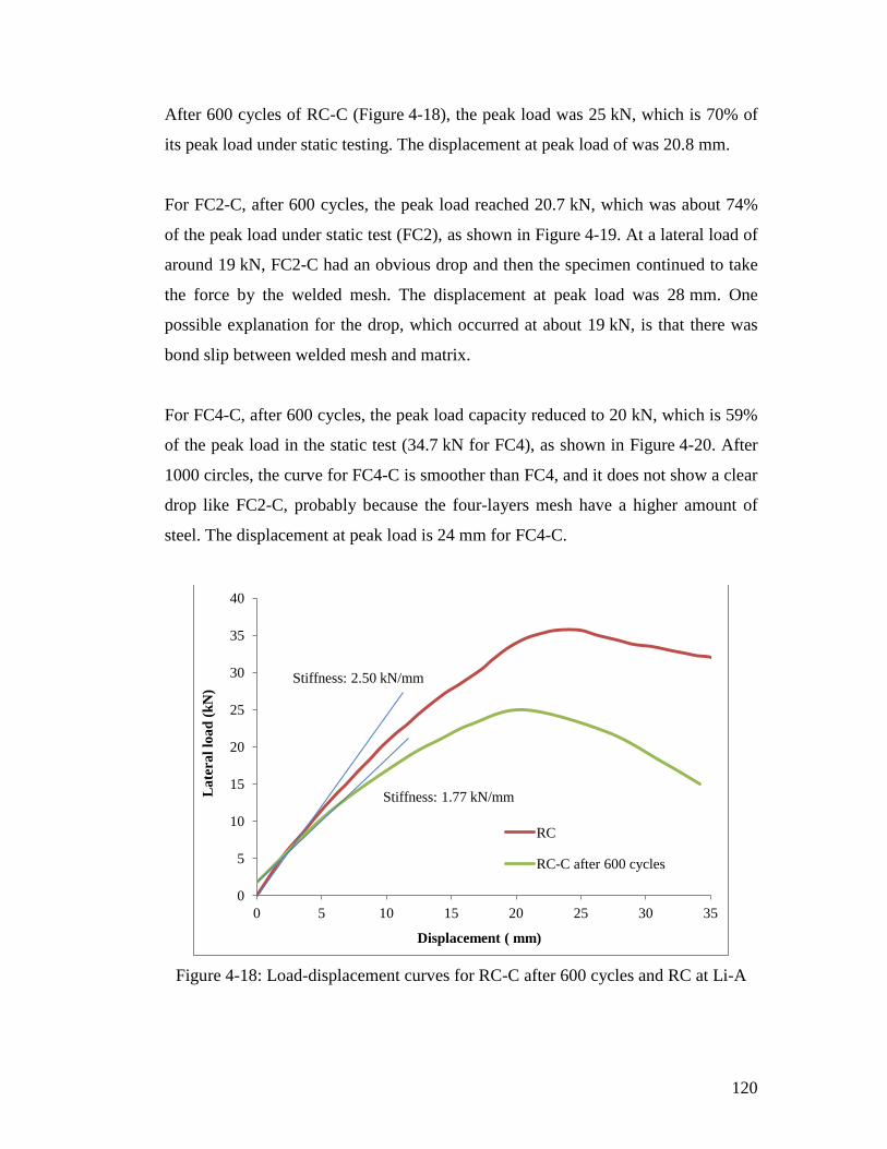
120

After 600 cycles of RC-C (Figure 4-18), the peak load was 25 kN, which is 70% of

its peak load under static testing. The displacement at peak load of was 20.8 mm.

For FC2-C, after 600 cycles, the peak load reached 20.7 kN, which was about 74%

of the peak load under static test (FC2), as shown in Figure 4-19. At a lateral load of

around 19 kN, FC2-C had an obvious drop and then the specimen continued to take

the force by the welded mesh. The displacement at peak load was 28 mm. One

possible explanation for the drop, which occurred at about 19 kN, is that there was

bond slip between welded mesh and matrix.

For FC4-C, after 600 cycles, the peak load capacity reduced to 20 kN, which is 59%

of the peak load in the static test (34.7 kN for FC4), as shown in Figure 4-20. After

1000 circles, the curve for FC4-C is smoother than FC4, and it does not show a clear

drop like FC2-C, probably because the four-layers mesh have a higher amount of

steel. The displacement at peak load is 24 mm for FC4-C.

Figure 4-18: Load-displacement curves for RC-C after 600 cycles and RC at Li-A

0

5

10

15

20

25

30

35

40

0 5 10 15 20 25 30 35

La

tera

l lo

ad

(k

N)

Displacement ( mm)

RC

RC-C after 600 cycles

Stiffness: 2.50 kN/mm


121


Li-A


Li-A

0

5

10

15

20

25

30

35

0 10 20 30 40

La

tera

l lo

ad

(k

N)

Displacement (mm)

FC2

FC2-C beforce cycle

FC2-C after 600 cycles



Bond slip

0

5

10

15

20

25

30

35

40

0 5 10 15 20 25 30 35 40

La

tera

l lo

ad

(k

N)

Displacement (mm)

FC4






122

Table 4-5: Peak load and displacement of specimens after cyclic load

Specimen Peak load

(kN) Peak load

degradation

Disp. at peak load

(mm)

RC 35.7

23.9

RC-C after 600

cycles 25 70% 20.8

FC2 29

20.9

FC2-C after 600

cycles 20.7 74% 28

FC4 34.7

22.7

FC4-C after 1000

cycles 20 59% 24

4.8 Deformation ductility results

The value of column deformation ductility is calculated as the ratio of deformation

at failure to deformation at yield. The energy balance method was used to create an

idealised bi-linear curve, the effective yield being at the turning point of the bi-linear

curve. The load-displacement diagram in Figure 4-21 shows the definition of the

deformation ductility, and this is given in Eq 4-3.

μ ) Eq 4-3

Where:


Displacement of the column in the descending branch

corresponding to 0.85 of the maximum load


123

Figure 4-21: The bi-linear idealization curve (FC2)

Figure 4-22 gives an example (FC2) of estimating the position of , which is

calculated using the area balance method (Barrera et al., 2012). The value of peak

load is 29 kN at 20.9 mm displacement ( ) . Using a three-degree polynomial

equation shows the specimen ascent stage (see Figure 4-22), as:

Where:

Displacement

Lateral load

So the area above the x-axis equals:

)

Put the value in equation, then:

0

5

10

15

20

25

30

35

0 5 10 15 20 25 30 35

La

tera

l lo

ad

(k

N)

Displacement (mm)

FC2

Bi-linear idealization curve of FC2

VPeak

0.85 VPeak

∆yI ∆u

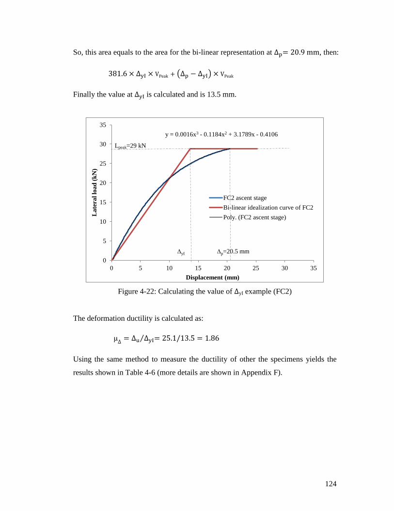
124

So, this area equals to the area for the bi-linear representation at , then:

Finally the value at is calculated and is 13.5 mm.

Figure 4-22: Calculating the value of ΔyI example (FC2)

The deformation ductility is calculated as:

μ

Using the same method to measure the ductility of other the specimens yields the

results shown in Table 4-6 (more details are shown in Appendix F).

y = 0.0016x3 - 0.1184x2 + 3.1789x - 0.4106

0

5

10

15

20

25

30

35

0 5 10 15 20 25 30 35

La

tera

l lo

ad

(k

N)

Displacement (mm)

FC2 ascent stage


Poly. (FC2 ascent stage)

∆yI ∆p=20.5 mm

Lpeak=29 kN

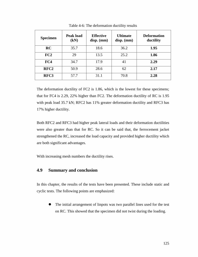
125

Table 4-6: The deformation ductility results

Specimen Peak load

(kN)

Effective

disp. (mm)

Ultimate

disp. (mm)

Deformation

ductility

RC 35.7 18.6 36.2 1.95

FC2 29 13.5 25.2 1.86

FC4 34.7 17.9 41 2.29

RFC2 50.9 28.6 62 2.17

RFC3 57.7 31.1 70.8 2.28

The deformation ductility of FC2 is 1.86, which is the lowest for these specimens;

that for FC4 is 2.29, 22% higher than FC2. The deformation ductility of RC is 1.95

with peak load 35.7 kN; RFC2 has 11% greater deformation ductility and RFC3 has

17% higher ductility.

Both RFC2 and RFC3 had higher peak lateral loads and their deformation ductilities

were also greater than that for RC. So it can be said that, the ferrocement jacket

strengthened the RC, increased the load capacity and provided higher ductility which

are both significant advantages.

With increasing mesh numbers the ductility rises.

4.9 Summary and conclusion

In this chapter, the results of the tests have been presented. These include static and

cyclic tests. The following points are emphasized:

The initial arrangement of linpots was two parallel lines used for the test

on RC. This showed that the specimen did not twist during the loading.

126

The displacement at top of the fixed-end plate was measured using two

extra linpots. The stiffness for each end of the fixed-end plate was

calculated, and it will be used in the ABAQUS modelling.

The peak load for the ferrocement and the deformation ductility depends

on the number of layers of mesh. More layers of mesh lead to higher

peak loads and greater values of deformation ductility.

The peak load for reinforced concrete strengthened using ferrocement

jacket was increased significantly.

During cyclic loading, the columns exhibit reduced load capacity for

constant deformation. After cyclic loading, the peak load reduced

significantly.

With higher amounts of mesh (FC4-C) the specimens showed lower load

reduction percentages for the same number of cycles.

The stiffness of RC-C dropped much quicker than that of the

ferrocement specimens.

The deformation ductility was calculated using the energy balanced

method. RFC3 had the highest ductility, and FC2 had the lowest.

127

CHAPTER 5 Finite element modelling

5.1 Introduction

Conducting column tests on ferrocement structures is time-consuming and expensive.

To avoid these problems, ABAQUS, a commercial FEM package, has been used by

researchers to study the behaviour of reinforced concrete structures. Due to the

similarity of ferrocement and reinforced concrete, and based on available literature,

ABAQUS has been used by the author in the present study.

ABAQUS has the ability to simulate complex structural behaviour under different

loading conditions, such as tension, compression, shear, etc. Complex detailed

models require significant computational resources. Ideally, the finite element model

needs to be kept as simple as possible. Because of the nature of the reinforcement in

ferrocement, a large amount of ferro-mesh including connections needs to be built

into each model. If a complete three-dimensional (3D) solid model is chosen for the

ferro-mesh, the model sizes and computational time will increase dramatically,

which is undesirable for research purposes. Also a 3D-solid detailed model is not

needed to capture the behaviour that is required in this study. Hence, a 3D non-linear

FE truss model was chosen for the ferro-mesh.

Compared to the welded mesh, the matrix requires less element refinement. Also in

ferrocement structures, the performance of the matrix influences the initial cracking

and ultimate strength in compression. So a 3D non-linear finite element analysis

approach is adopted for the ferro-matrix to provide a simulation that is more detailed

and to provide results that are more accurate. The type of elements selected for

matrix and ferro-mesh affect both the accuracy and the time taken for the

computation.

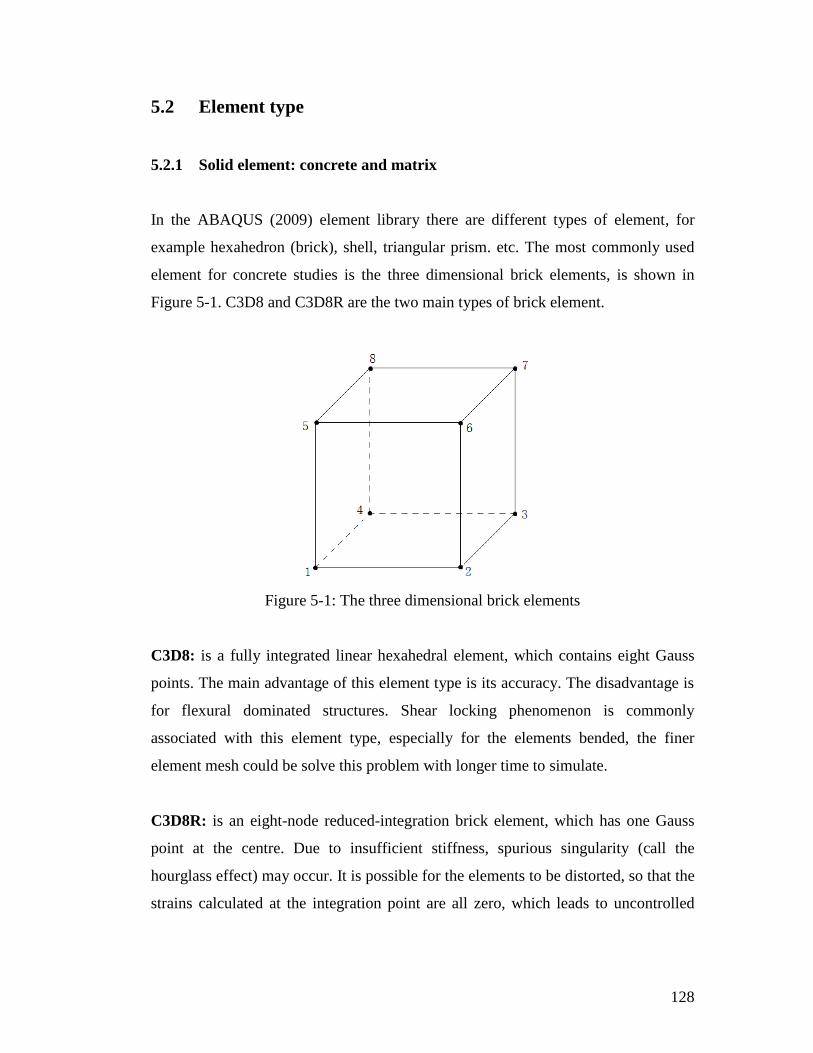
128

5.2 Element type

5.2.1 Solid element: concrete and matrix

In the ABAQUS (2009) element library there are different types of element, for

example hexahedron (brick), shell, triangular prism. etc. The most commonly used

element for concrete studies is the three dimensional brick elements, is shown in

Figure 5-1. C3D8 and C3D8R are the two main types of brick element.

Figure 5-1: The three dimensional brick elements

C3D8: is a fully integrated linear hexahedral element, which contains eight Gauss

points. The main advantage of this element type is its accuracy. The disadvantage is

for flexural dominated structures. Shear locking phenomenon is commonly

associated with this element type, especially for the elements bended, the finer

element mesh could be solve this problem with longer time to simulate.

C3D8R: is an eight-node reduced-integration brick element, which has one Gauss

point at the centre. Due to insufficient stiffness, spurious singularity (call the

hourglass effect) may occur. It is possible for the elements to be distorted, so that the

strains calculated at the integration point are all zero, which leads to uncontrolled

129

distortion of the mesh. In order to control this, an artificial stiffness method and

artificial damping method in the ABAQUS code is proposed.

For this thesis, the element used for concrete and the matrix was C3D8R. Using

C3D8R underestimates the failure load slightly, but it is less time consuming, shear

lock problems can be avoided and good results are obtained by adopting fine meshes.

5.2.2 Truss element: steel bar, stirrup and welded mesh

The reinforcement materials, including ribbed bars, stirrups and the welded mesh,

are modelled using the T3D2 truss elements. These are two-node three dimensional

straight truss elements.

5.3 Concrete damaged plasticity model

The concrete damaged plasticity (CDP) model is capable of capturing the

behaviour of concrete and quasi-brittle materials. The inelastic behaviour of

concrete can be incorporated using isotropic damage elasticity in combination

with the isotropic tension and the compression plasticity. The model considers

the degradation of the elastic stiffness due to tensile and compressive plastic

straining.

The material property input in ABAQUS is in two groups, uniaxial stress-

strain curves and plasticity parameters. These are shown in the following

sections:

5.3.1 Concrete under uniaxial compression

Figure 5-2 shows the response of concrete under uniaxial compressive loading. The

concrete will behave linearly until its stress reaches initial yield ( ). Beyond

130

hardening is developed in the concrete and then, after reaching the ultimate stress

( ), strain softening is observed.


in compression (ABAQUS, 2009)

Where:

Compression stress of concrete

Compression yield stress

Ultimate compression stress

Compression strain

Elastic compressive strain

Plastic compressive strain

Compressive damage variable

The damaged variables ( ) help describe the effect of stiffness recovery during

cyclic loading and degradation in the elastic stiffness of concrete. The damaged

variables correlate with the plastic strains (

). The magnitude of the damage

131

variables range from 0 to 1; with 0 representing the undamaged material and 1

meaning the total loss of material strength.

Therefore, to interpret the concrete damaged plasticity (CDP) model accurately, the

compressive behaviour, tensile behaviour and plasticity, need to be considered.

5.3.2 Compressive behaviour for CDP

Compressive behaviour is defined as: the uniaxial compressive response of plain

material beyond its elastic range. The inelastic strain is shown in ABAQUS (2009)

documentation and is calculated as Eq 5-1:

Eq 5-1

Where:

Inelastic compressive strain of concrete

Elastic compressive strain of concrete at yield,

Two uniaxial compressive stress-strain models have been used in this thesis:

Eurocode 2 (CEN, 2004a) and Popovics (1973).

5.3.2.1 Eurocode 2 concrete material model:

Figure 5-3 shows the relationship between stress and strain for concrete under

uniaxial compression; the mathematical expression of which is given in Eq 5-2.

132

Figure 5-3: The stress-strain curve for concrete under uniaxial compression for

Eurocode 2 (CEN, 2004a)

Where:

Concrete cylinder compressive strength

Compressive strain at peak stress,

Ultimate strain,

Young's modulus of concrete, )

The equation of this curve is:

η η

)η Eq 5-2

Where:

η Ratio of compression strain with strain at peak load,

=

133

Figure 5-4 shows the use of the previous equation (Eq 5-2) to simulate the

experimental data, which predicted the property of concrete.

Figure 5-4: Comparison of prediction (Eq 5-2) and experimental results (Eurocode 2

model for compressive concrete property)

5.3.2.2 Popovics model for matrix material:

For the matrix cylinder compressive stress-strain relationship, the equation proposed

by Popovics (1973) is shown in Eq 5-3. Experimental values of peak stress ( ) and

the related strain ( ) were used in this equation, and it was found that the matrix

property curve was close to the experimental result, as shown in Figure 5-5. The post

peak stage is important for the property of the confined matrix input in ABAQUS,

and it will affect the accuracy of the FEM.

0

5

10

15

20

25

30

35

40

0 0.001 0.002 0.003 0.004 0.005 0.006

Str

ess

(MP

a)

Strain

Experimental result

Prediction

134

)

) Eq 5-3

Where:


Peak compressive strength

Compressive strain

Compressive strain at peak stress

Approximate function of compressive strength of matrix,

Figure 5-5: Comparison of prediction (Eq 5-3) and experimental results (Popovics

model for compressive matrix property)

Therefore, Eq 5-3 is adopted for the parametric studies. To use this formula,

two variables need to be selected: peak stress ( ) and its relative strain ( ),

a statistical approach based on experimental results was made as shown in

Figure 5-6 (Tian, 2013). The resulting expression is given in Eq 5-4.

135

Figure 5-6: The curve fit for peak compressive stress and strain of matrix (Tian,

2013)

Note: Author and Tian cast and test the cylinders together, but Tian analysed the results.

Therefore, the equation as shown:

) Eq 5-4

5.3.3 Concrete under uniaxial tension

The stress-strain curve for concrete under uniaxial tension is shown in Figure 5-7. In

the first stage of loading concrete will experience linear elastic behaviour until the

failure stress ( ) is reached. The failure stress corresponds to micro-cracking that

occurs in the concrete. Beyond (second stage), the micro cracks continue to

increase and this can be denoted as the softening the response of stress-strain

relationship.

y = -1.24E-05x + 4.31E-03

0.0034

0.0035

0.0036

0.0037

0.0038

0.0039

0.004

20 30 40 50 60 70

Str

ain

Peak compression stress (MPa)

The peak compressive stress

Linear (The peak compressive stress)

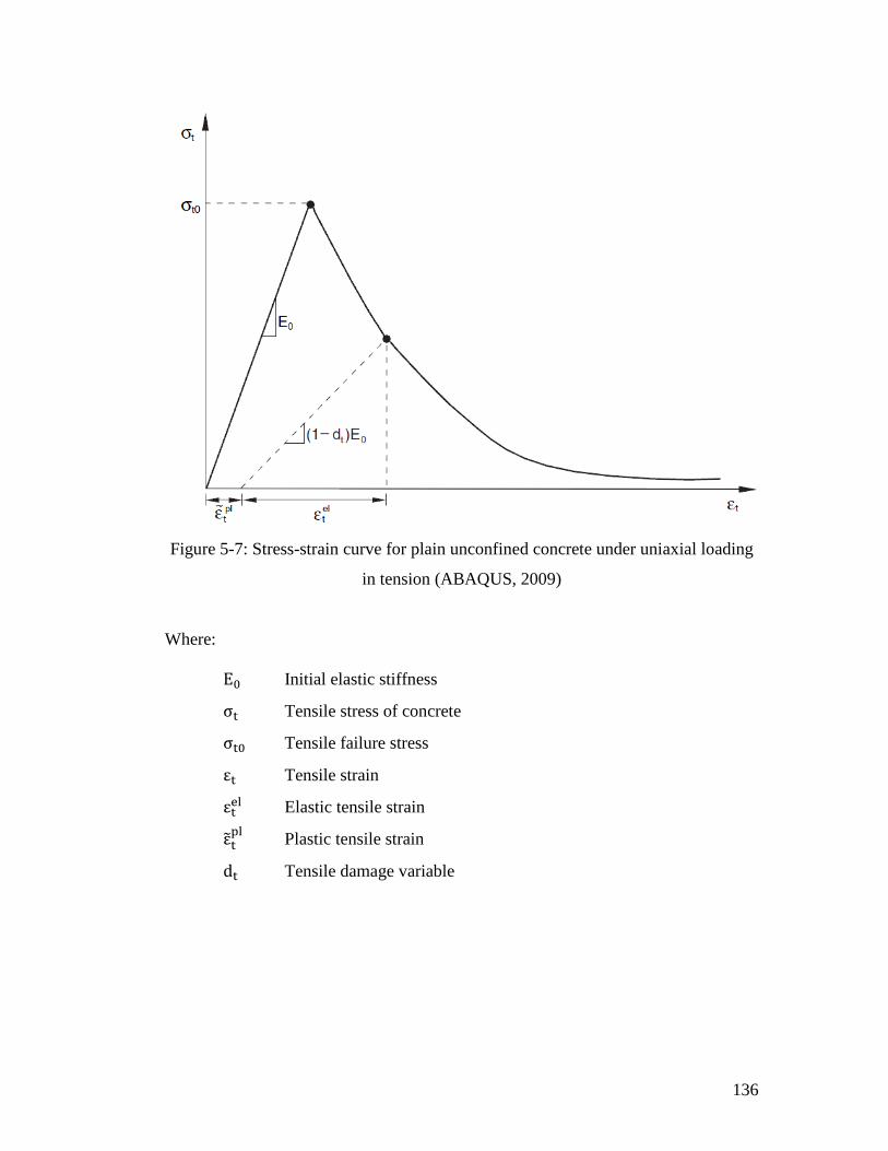
136


in tension (ABAQUS, 2009)

Where:

Initial elastic stiffness


Tensile failure stress

Tensile strain

Elastic tensile strain

Plastic tensile strain

Tensile damage variable

137

5.3.4 Tensile behaviour for CDP

The tensile behaviour of concrete or the matrix is defined as the uniaxial tensile

response of the material in its post-failure range. The cracking strain is calculated

shows in Eq 5-5.

Eq 5-5

Where:

Cracking strain of concrete

Elastic tensile strain of concrete at yield,

Wang and Hsu (2001) reported a uniaxial tensile stress-strain curve. This value was

used for input to ABAQUS for both the tensile property of concrete and the matrix.

Eq 5-6 shows the relationship between the cracking strain and stress.

The split tests of cylinder results are shown in § 3.2.3, the ultimate stress for

concrete reached 3.74 N/mm2, for matrix reached 4.44 N/mm

2, the stress-strain

curves of tensile concrete and matrix properties is shown in Figures 5-8 and 5-9

respectively.

) Eq 5-6

Where:


Strain at cracking,

The relationship between the ultimate tensile stress ( ) and compressive stress

( ) is shown in Figure 5-10, where the curve fitting approach is based on

experimental results (Tian, 2013). The equation used is shown in Eq 5-7.

138

Figure 5-8: Tensile stress-strain curve of concrete based on Eq 5-6 (3.74 N/mm2 for

concrete tensile stress)

Figure 5-9: Tensile stress-strain curve of matrix based on Eq 5-6 (4.44 N/mm2 for

matrix tensile stress)

0

1

2

3

4

5

0.000 0.000 0.001 0.001 0.002 0.002 0.003 0.003 0.004

Str

ess

(MP

a)

Strain

0

1

2

3

4

5

0.000 0.000 0.001 0.001 0.002 0.002 0.003 0.003 0.004

Str

ess

(MP

a)

Strain

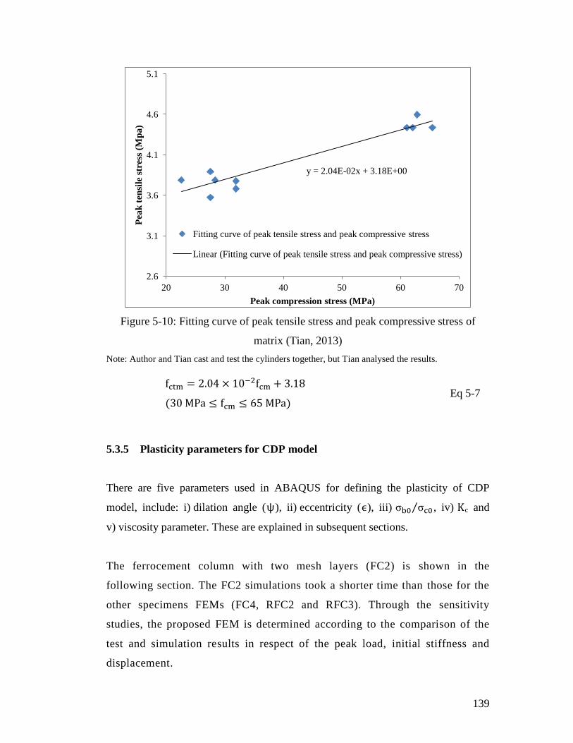
139

Figure 5-10: Fitting curve of peak tensile stress and peak compressive stress of

matrix (Tian, 2013)

Note: Author and Tian cast and test the cylinders together, but Tian analysed the results.

) Eq 5-7

5.3.5 Plasticity parameters for CDP model

There are five parameters used in ABAQUS for defining the plasticity of CDP

model, include: i) dilation angle (ψ), ii) eccentricity ( ), iii) σ σ , iv) c and

v) viscosity parameter. These are explained in subsequent sections.

The ferrocement column with two mesh layers (FC2) is shown in the

following section. The FC2 simulations took a shorter time than those for the

other specimens FEMs (FC4, RFC2 and RFC3). Through the sensitivity

studies, the proposed FEM is determined according to the comparison of the

test and simulation results in respect of the peak load, initial stiffness and

displacement.

y = 2.04E-02x + 3.18E+00

2.6

3.1

3.6

4.1

4.6

5.1

20 30 40 50 60 70

Pea

k t

ensi

le s

tres

s (M

pa

)

Peak compression stress (MPa)

Fitting curve of peak tensile stress and peak compressive stress

Linear (Fitting curve of peak tensile stress and peak compressive stress)

140

In ABAQUS, the Drucker-Prager hyperbolic function (Drucker and Prager, 2013) is

used to define non-associated (not identical with the yield surface) potential plastic

flow for concrete damage plasticity (CDP). The potential plastic flow (G), which is

continuous and smooth, is shown in Figure 5-11. The equation of the curve is

presented in Eq 5-8.

Figure 5-11: The hyperbolic potentials in the meridional stress plane

ψ) ψ Eq 5-8

Where:

ψ The dilation angle measured in the p–q plane at high confining

pressure

Eccentricity, defined as the rate of plastic potential function

approaches at the asymptote line. The default is

The uniaxial tensile stress at failure, taken from the user-specified

tension stiffening data

G The potential plastic flow

p The effective hydrostatic stress

q The Von Mises equivalent effective stress

ψ

σ

141

5.3.5.1 Dilation angle (ψ)

The dilation angle (ψ) measures the inclination of the plastic strain at a high

confining pressure. A material with a low value of this angle experiences

brittle behaviour, whereas high values indicate that the material has a high

ductile behaviour. To decide on the value of ψ, a sensitivity test was carried

out and the results were compared with the experimental results. This is

shown in Figure 5-12. From this, a dilation angle of 49° is the best fit for the

test results, as the load-displacement curve was found to be closest to

experimental result.

Figure 5-12: Comparison of FEM load-displacement curves using different dilation

angles and the experimental result (FC2)

0

5

10

15

20

25

30

35

0 5 10 15 20 25 30 35 40

La

tera

l lo

ad

(k

N)

Displacement (mm)

Test 20 degree

30 degree 40 degree

49 degree (used) 50 degree

54 degree

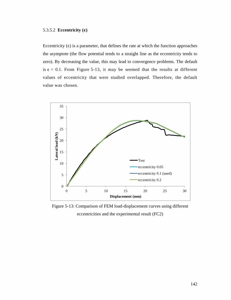
142

5.3.5.2 Eccentricity ( )

Eccentricity ( ) is a parameter, that defines the rate at which the function approaches

the asymptote (the flow potential tends to a straight line as the eccentricity tends to

zero). By decreasing the value, this may lead to convergence problems. The default

is = 0.1. From Figure 5-13, it may be seemed that the results at different

values of eccentricity that were studied overlapped. Therefore, the default

value was chosen.

Figure 5-13: Comparison of FEM load-displacement curves using different

eccentricities and the experimental result (FC2)

0

5

10

15

20

25

30

35

0 5 10 15 20 25 30

La

tera

l lo

ad

(k

N)

Displacement (mm)

Test

eccentricity 0.05

eccentricity 0.1 (used)

eccentricity 0.2

143

5.3.5.3 σbo/σco

The ratio of initial equi-biaxial compressive yield stress to initial uniaxial

compression yield stress is required as an input to ABAQUS. Figure 5-14

shows the effect of changing the value of . Again, the results show

negligible differences, hence the default input value of 1.16 was chosen.

Figure 5-14: Comparison of FEM load-displacement curves using different σbo/σco

values and experimental result (FC2)

0

5

10

15

20

25

30

35

0 5 10 15 20 25 30

La

tera

l lo

ad

(k

N)

Displacement (mm)

Test

fb0/fc0=1.10

fb0/fco=1.16 (used)

fb0/fc0=1.20

Test

σbo/σco=1.10

σbo/σco=1.16 (used)

σbo/σco=1.20

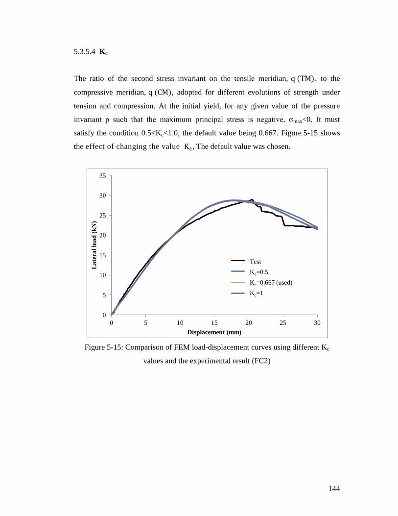
144

5.3.5.4 Kc

The ratio of the second stress invariant on the tensile meridian, ), to the

compressive meridian, ), adopted for different evolutions of strength under

tension and compression. At the initial yield, for any given value of the pressure

invariant p such that the maximum principal stress is negative, σmax<0. It must

satisfy the condition 0.5<Kc<1.0, the default value being 0.667. Figure 5-15 shows

the effect of changing the value , The default value was chosen.

Figure 5-15: Comparison of FEM load-displacement curves using different Kc

values and the experimental result (FC2)

0

5

10

15

20

25

30

35

0 5 10 15 20 25 30

La

tera

l lo

ad

(k

N)

Displacement (mm)

Test

Kc=0.5

Kc=0.667 (used)

Kc=1

Test

Kc=0.5

Kc=0.667 (used)

Kc=1

145

5.3.5.5 Viscosity parameter

The viscosity parameter (μ) is defined in ABAQUS to represent the relaxation time

of the visco-plastic system. By changing this value, the length of the experimental

simulation time for each step may be influenced. Moreover, the softening behaviour

and stiffness degradation behaviour of the material models may be influenced.

Instead of changing the viscosity parameter and step time simultaneously, the step

time was set as a constant value and the viscosity parameter was varied. Also by

defining a small number μ in ABAQUS, convergence difficulties were overcome.

As shown in Figure 5-16, a viscosity parameter of 0.055 gives the best-fit curve to

the experimental curve, so 0.055 was chosen in this study.


parameters and the experimental result (FC2)

0

5

10

15

20

25

30

35

0 5 10 15 20 25 30

La

tera

l lo

ad

(k

N)

Displacement (mm)

Test viscosity=0.01

viscosity=0.03 viscosity=0.05

viscosity=0.055 (used) viscosity=0.06

146

In summary, the five coefficients used for modelling the plasticity of the matrix and

concrete are tabulated in Table 5-1. For the concrete parameters, the default values

shown in Table 5-1 are used, except the viscosity parameter value. The results vary

with the viscosity parameter value as shown in Figure 5-17. The best-fit curve is

when the viscosity equals 0.015.

Table 5-1: Coefficients for ferrocement and concrete column

Material Dilation

Angle ( ) Eccentricity

( ) σb0/σc0 Kc

Viscosity

parameter (μ)

Matrix 49 0.1 1.16 0.667 0.055

Concrete 30 0.1 1.16 0.667 0.015


parameters and the experimental result (RC)

0

5

10

15

20

25

30

35

40

0 5 10 15 20 25 30 35 40

La

tera

l lo

ad

(k

N)

Displacement (mm)

Test RC

viscosity=0.005

viscosity=0.01

viscosity=0.015 (used)

viscosity=0.02

147

5.4 Contact

When considering reinforced materials to ensure physical contact, different linking

methods are available. Two types of constraint were selected in this thesis; the

embedded region constraint and the “Tie” constraint.

5.4.1 Embedded region

Reinforcement in concrete structures is typically provided by rebar. Normally the

rebars are defined as one-dimensional wire truss elements and the reinforcement can

be defined in ABAQUS using a single wire. In this thesis, a metal plasticity model

was used, which presents elastic-perfectly plastic behaviour for reinforcement.

The concrete behaviour is independent of the reinforcement behaviour, so the

interaction between concrete and reinforcement, the embedded bond (perfect bond),

was defined in this studies to simulate load transfer between concrete and

reinforcement. In addition, the welded mesh was also embedded in the matrix

structure.

5.4.2 Tie constraint

When concrete columns are strengthened using ferrocement material, the

constraint between the concrete surface and the matrix surface was chosen to

be a “Tie” constraint in ABAQUS. To use this constraint, some basic rules

must be followed. In principle, the master surface should be applied to the

stronger material compared with the material using the slave surface.

Therefore, the concrete surface can be defined as the master face, whereas the

matrix surface should be the slave face during the whole simulation.

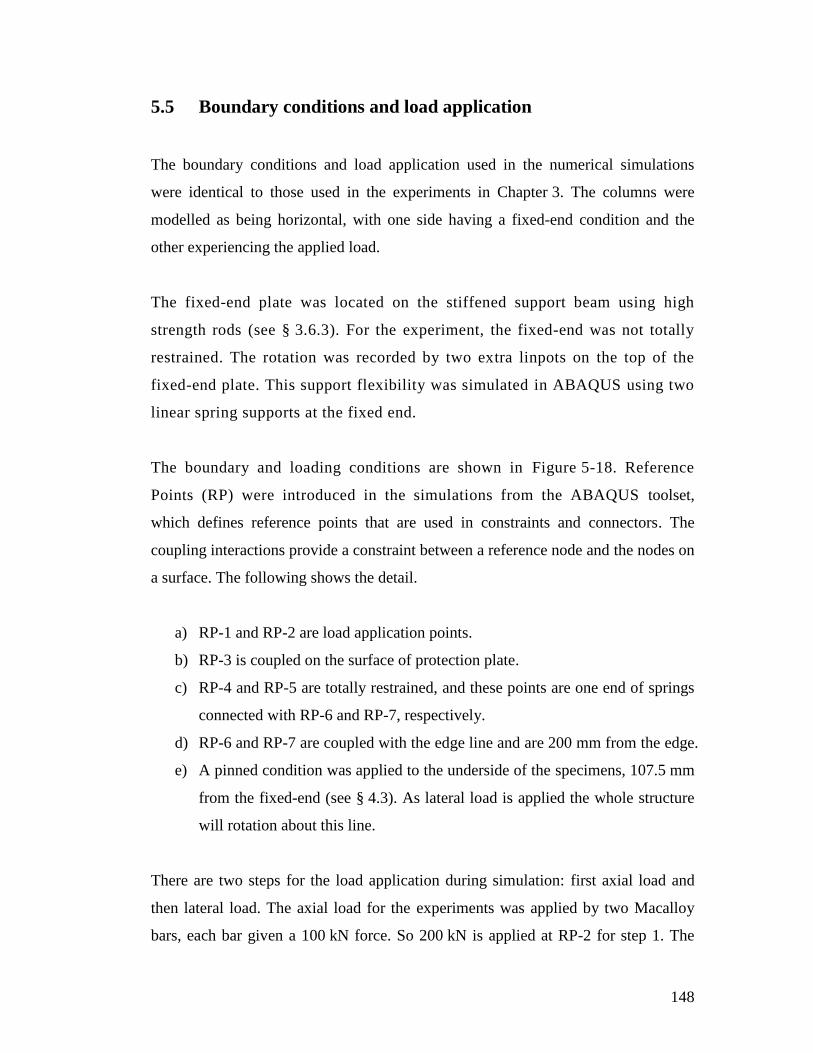
148

5.5 Boundary conditions and load application

The boundary conditions and load application used in the numerical simulations

were identical to those used in the experiments in Chapter 3. The columns were

modelled as being horizontal, with one side having a fixed-end condition and the

other experiencing the applied load.

The fixed-end plate was located on the stiffened support beam using high

strength rods (see § 3.6.3). For the experiment, the fixed-end was not totally

restrained. The rotation was recorded by two extra linpots on the top of the

fixed-end plate. This support flexibility was simulated in ABAQUS using two

linear spring supports at the fixed end.

The boundary and loading conditions are shown in Figure 5-18. Reference

Points (RP) were introduced in the simulations from the ABAQUS toolset,

which defines reference points that are used in constraints and connectors. The

coupling interactions provide a constraint between a reference node and the nodes on

a surface. The following shows the detail.

a) RP-1 and RP-2 are load application points.

b) RP-3 is coupled on the surface of protection plate.

c) RP-4 and RP-5 are totally restrained, and these points are one end of springs

connected with RP-6 and RP-7, respectively.

d) RP-6 and RP-7 are coupled with the edge line and are 200 mm from the edge.

e) A pinned condition was applied to the underside of the specimens, 107.5 mm

from the fixed-end (see § 4.3). As lateral load is applied the whole structure

will rotation about this line.

There are two steps for the load application during simulation: first axial load and

then lateral load. The axial load for the experiments was applied by two Macalloy

bars, each bar given a 100 kN force. So 200 kN is applied at RP-2 for step 1. The

149

lateral load was applied by the actuator, under displacement control, so for the

simulation, displacement was applied at RP-1 for step 2.

Figure 5-18: The boundary conditions and loading applications

Two linear springs were added at the fixed-end to simulate the rotations observed for

the whole specimen (see § 4.3). The value of spring stiffnesses by hand calculation

are: 85.6 kN/mm and 127 kN/mm (see § 4.3).

5.6 Detail description of reinforcement in ABAQUS

The reinforcement of RC, FC and RFC in ABAQUS simulation is exactly same

position and amount as experimental specimens, shown in Figures 5-19, 5-20 and

5-21.

Spring 2

Step 1: Axial load

Step 2: Lateral load

Total restraint

Spring 1

RP-3

RP-4

RP-5

RP-2

RP-6

RP-7

RP-1

Rigid body surface

Pin end

150

Figure 5-19: The reinforcement of RC

Figure 5-20: The reinforcement of FC

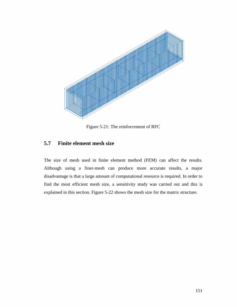
151

Figure 5-21: The reinforcement of RFC

5.7 Finite element mesh size

The size of mesh used in finite element method (FEM) can affect the results.

Although using a finer-mesh can produce more accurate results, a major

disadvantage is that a large amount of computational resource is required. In order to

find the most efficient mesh size, a sensitivity study was carried out and this is

explained in this section. Figure 5-22 shows the mesh size for the matrix structure.

152

Figure 5-22: The mesh size for the matrix

Figure 5-23 shows the simulation results for FC2 using different mesh sizes for the

matrix. It is clear that the four different mesh sizes produce the same initial stiffness,

however, the 20 mm mesh size generated the closest results to the test results on the

descent part, with a computational CPU time of 523 minutes. In comparison with

this, using 30 mm mesh size produces similar results, but the calculation time

reduced to 143 minutes. Therefore, the 30 mm mesh size for the matrix was selected.

Table 5-2 presented the effects of different element sizes of matrix on the numerical

simulation for FC2.

(a): mesh size 50 mm (b): mesh size 40 mm

(c): mesh size 30 mm (d): mesh size 20 mm

153

Figure 5-23: The mesh size for the matrix (FC2)

Table 5-2: Mesh sensitivity study for matrix mesh size

Matrix mesh

size(mm)

Number of

elements

Simulation time

(CPU mins)

Test load

(kN)

Simulation

load (kN)

20 3264 523

29.5

29.4

30 875 143 29.1

40 416 85 28.0

50 180 58 27.6

Then, the author simulated varying with the mesh size of reinforcing mesh, shows in

Figure 5-24, and results presents in Table 5-3. The results show the 12.6 mm mesh

size have same value with the mesh size equal 6.3 mm. So finally, the 12.6 mm

mesh size for mesh reinforcement was selected.

0

5

10

15

20

25

30

35

0 5 10 15 20 25 30 35

La

tera

l lo

ad

(k

N)

Displacement (mm)

Test FC2

Mesh size 20 mm

Mesh size 30 mm (used)

Mesh size 40 mm

Mesh size 50 mm

154

Figure 5-24: The mesh size of reinforcement (FC2)

Table 5-3: Mesh sensitivities for reinforcing mesh size with concrete size 30 mm

Welded mesh

size (mm)

Number of

elements

Simulation time

(CPU mins)

Test load

(kN)

Simulation

load (kN)

12.6 14976 143 29.5

29.1

6.3 29952 501 29.0

5.8 Verification of FEM with experiments

Verification of the FEM results using the experimental results is given in the

following sections. The load-deflection response of the columns under

combination of axial load and bending were shown in Chapter 3. A good

agreement was found between the FEM results and the experimental results as

described in the following sections, especially in the ascending stages and

peak loads for all numerical simulations, but with slight differences on the

descending part. Three groups of FEM results are compared with the

experiment results:

0

5

10

15

20

25

30

35

0 5 10 15 20 25 30 35

La

tera

l lo

ad

(k

N)

Displacement (mm)

Test FC2

Reinforcing mesh 12.6 mm (used)

Reinforcing mesh 6.3 mm

155

a) Reinforced concrete column (RC)

b) Ferrocement columns (FC)

c) Reinforced concrete columns strengthened using a ferrocement jacket (RFC)

5.8.1 Reinforced concrete column

A comparison between the FEM analysis results and the experimental results for RC

is shown in Figure 5-26. The values and deviations are presented in Table 5-4. The

deviation is calculated using Eq 5-1; notice that the deviations of initial stiffness for

all specimens are calculated at a lateral applied load of 10 kN. The deviation of

peak load was 3% lower and displacement at peak load was 6% higher.

Eq 5-1

In Figure 5-26, it may be seen that the simulation results are close to the test

results despite the maximum load obtained from FEM being smaller. It is

worth mentioning that the test load dropped suddenly when the column

deflection reached 39 mm, however the curve in the simulation gradually

decreased. There are two loads of particular interest, namely the peak load

and 85% post peak.

The FEM details of FC column at peak load and 85% post peak load are

shown in Figure 5-27.

Figure 5-25 is the display and describe of the Figures 5-27, 5-30, 5-31, 5-34 and

5-35.

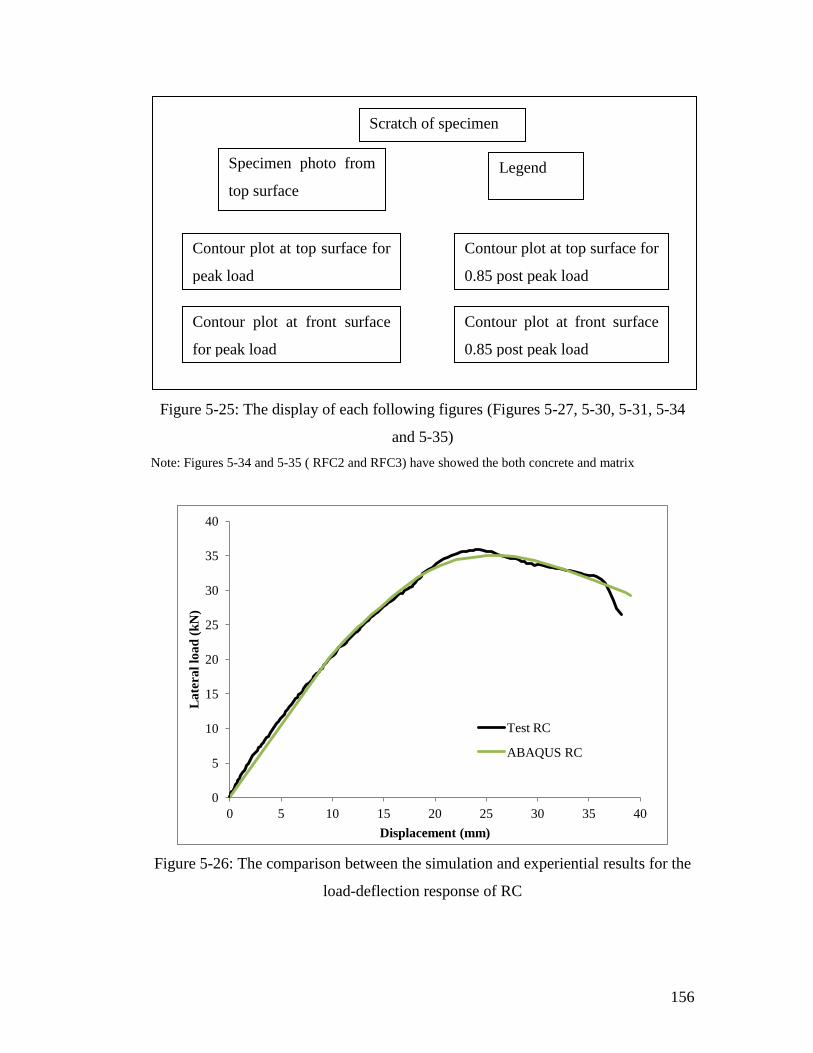
156

Figure 5-25: The display of each following figures (Figures 5-27, 5-30, 5-31, 5-34

and 5-35)

Note: Figures 5-34 and 5-35 ( RFC2 and RFC3) have showed the both concrete and matrix


load-deflection response of RC

0

5

10

15

20

25

30

35

40

0 5 10 15 20 25 30 35 40

La

tera

l lo

ad

(k

N)

Displacement (mm)

Test RC

ABAQUS RC

Scratch of specimen

Specimen photo from

top surface

Legend

Contour plot at top surface for

peak load

Contour plot at front surface

for peak load

Contour plot at top surface for

0.85 post peak load

Contour plot at front surface

0.85 post peak load

157

Table 5-4: Comparison of test and FEM (RC)

Specimen RC

Test FEM Deviation

Peak load (kN) 35.7 34.6 -3%

Displacement at peak load

(mm) 23.9 25.3 6%

Stiffness (kN/mm) 2.50 2.13 -12%

At the peak load, the maximum principal strain occurs on the top surface and

reached 0.009. This produced cracks round the top surface. After the peak load, the

strain of the concrete significantly increases, and at 85% post peak load it reached

0.0186.

158


0.0186 for 0.85 post peak load (RC)

Note: Test picture is taken approximately before the lateral peak load has been reached

5.8.2 Ferrocement columns

FEM results for the ferrocement columns are in good agreement with experiments as

seen in Figures 5-28 and 5-29. Table 5-5 presents the difference between the FEM

results and the test results.

In Figure 5-28, the linear part of the FEM result is slightly softer than that from the

experiment; the initial stiffness for the FEM is 2.35 with a deviation that is 9.6%

Peak load 85% post peak load

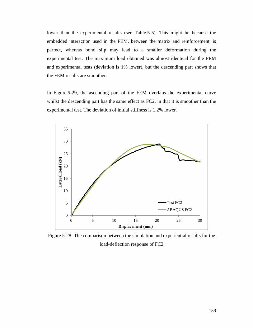
159

lower than the experimental results (see Table 5-5). This might be because the

embedded interaction used in the FEM, between the matrix and reinforcement, is

perfect, whereas bond slip may lead to a smaller deformation during the

experimental test. The maximum load obtained was almost identical for the FEM

and experimental tests (deviation is 1% lower), but the descending part shows that

the FEM results are smoother.

In Figure 5-29, the ascending part of the FEM overlaps the experimental curve

whilst the descending part has the same effect as FC2, in that it is smoother than the

experimental test. The deviation of initial stiffness is 1.2% lower.


load-deflection response of FC2

0

5

10

15

20

25

30

35

0 5 10 15 20 25 30

La

tera

l lo

ad

(k

N)

Displacement (mm)

Test FC2

ABAQUS FC2

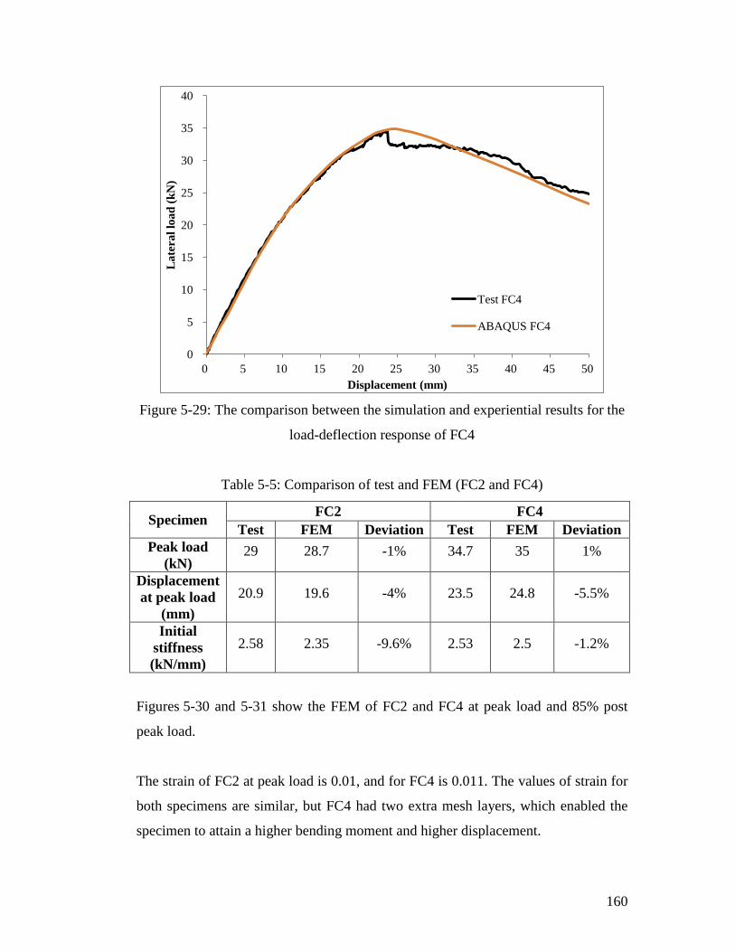
160


load-deflection response of FC4

Table 5-5: Comparison of test and FEM (FC2 and FC4)

Specimen FC2 FC4

Test FEM Deviation Test FEM Deviation

Peak load

(kN) 29 28.7 -1% 34.7 35 1%

Displacement

at peak load

(mm)

20.9 19.6 -4% 23.5 24.8 -5.5%

Initial

stiffness

(kN/mm)

2.58 2.35 -9.6% 2.53 2.5 -1.2%

Figures 5-30 and 5-31 show the FEM of FC2 and FC4 at peak load and 85% post

peak load.

The strain of FC2 at peak load is 0.01, and for FC4 is 0.011. The values of strain for

both specimens are similar, but FC4 had two extra mesh layers, which enabled the

specimen to attain a higher bending moment and higher displacement.

0

5

10

15

20

25

30

35

40

0 5 10 15 20 25 30 35 40 45 50

La

tera

l lo

ad

(k

N)

Displacement (mm)

Test FC4

ABAQUS FC4

161

At 85% post peak load, the strain of FC2 reached 0.0202, and for FC4 was 0.0225.

In addition, the peak strains for each FEM are shown at the top surface, where

cracks were observed.

Figure 5-30: The PE, Max. Principal at peak load of FEM, 0.01 at peak load, 0.0202

for 0.85 post peak load (FC2)

Note: Test picture is taken approximately after the lateral peak load has been reached

Peak load 0.85 post peak load

162


0.0268 for 0.85 post peak load (FC4)


5.8.3 Reinforced concrete columns strengthened using ferrocement jackets

The good agreement of the FEM results and the experimental results for both

columns (RFC2 and RFC3) is shown in Figures 5-32 and 5-33. The deviations are

shown in Table 5-6. The initial ascending part of the FEMs had slightly higher initial

stiffness (deviation for RFC2 is 22% higher and for RFC3 is 20% higher), but after

Peak load 0.85 post peak load

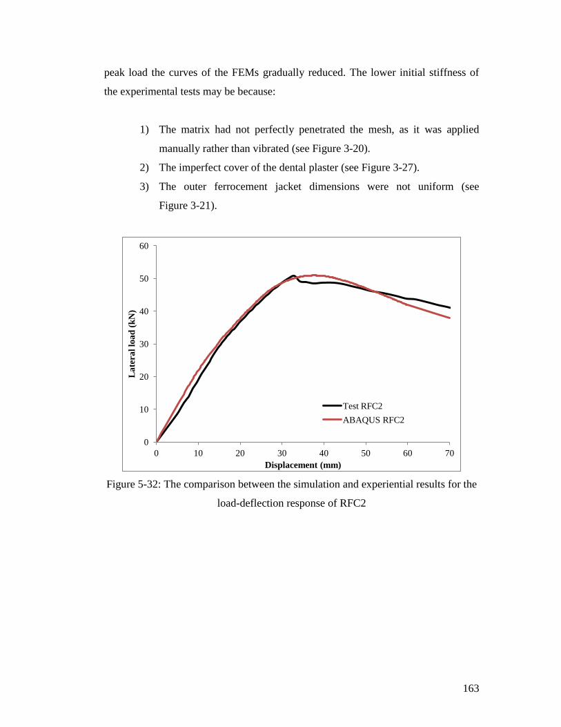
163

peak load the curves of the FEMs gradually reduced. The lower initial stiffness of

the experimental tests may be because:

1) The matrix had not perfectly penetrated the mesh, as it was applied

manually rather than vibrated (see Figure 3-20).

2) The imperfect cover of the dental plaster (see Figure 3-27).

3) The outer ferrocement jacket dimensions were not uniform (see

Figure 3-21).


load-deflection response of RFC2

0

10

20

30

40

50

60

0 10 20 30 40 50 60 70

La

tera

l lo

ad

(k

N)

Displacement (mm)

Test RFC2

ABAQUS RFC2

164


load-deflection response of RFC3

Table 5-6: Comparison of test and FEM (RFC2 and RFC3)

Specimen RFC2 RFC3

Test FEM Deviation Test FEM Deviation

Peak load

(kN) 50.8 51 0% 57.5 58.1 1%

Displacement

at peak load

(mm)

33.6 37.5 12% 39.2 42.5 8%

Initial

stiffness

(kN/mm)

1.7 2.1 22% 2.0 2.4 20%

0

10

20

30

40

50

60

70

0 10 20 30 40 50 60 70

La

tera

l lo

ad

(m

m)

Displacement (mm)

Test RFC3

ABAQUS RFC3

165

Figures 5-34 and 5-35 show the RFC2 and RFC3 FEM at peak load and 85% post

peak load. Each simulation represents the inner reinforced concrete and the outer

ferrocement.

RFC2: At the peak load, the strain of reinforced concrete reached 0.0093, and

outer ferrocement 0.0288, the ferrocement layer acted as confinement. At

85% post peak load, the ferrocement strain reached 0.0651, many cracks were

present on the top surface, and front and back surfaces.

RFC3: The behaviour of RFC3 was similar to RFC2, at peak load, the strain

of inner reinforced concrete was 0.0099, and outer ferrocement 0.0305. At

85% post peak load, the ferrocement strain reached 0.0544, which is lower

than that for RFC2.

166


0.0268 for 0.85 post peak load (RFC2)

Note: Test picture is taken approximately after the lateral peak load has been reached

Peak load for matrix 0.85 post peak load for matrix

Peak load for concrete 0.85 post peak load for concrete

167


0.0268 for 0.85 post peak load (RFC3)


Peak load for concrete 0.85 post peak load for concrete

Peak load for matrix 0.85 post peak load for matrix

168

5.9 Ductility of FEM compared with experimental tests

The deformation ductility of each simulation is shown in Table 5-7. RFC2 has the

same value as the experimental test (2.20). FC2 had quite a different value from the

experimental test. For FC2: after the peak load, the load of the experimental test

drops quickly, but the simulation could not properly represent the descent stage, as

the simulation had a smooth decrease load after peak load.

Table 5-7: Deformation ductility comparison of test results and FEM

Name Type

Peak

load

(kN)

Effective

displacement

(mm)

Ultimate

displacement

(mm)

Deformation

ductility

RC Test 35.7 21.6 37.5 1.74

FEM 35.0 20.9 38.5 1.83

FC2 Test 28.0 13.5 25.1 1.74

FEM 28.7 14.0 28.8 2.05

FC4 Test 34.7 16.8 41.0 2.44

FEM 35.0 16.5 39.5 2.40

RFC2 Test 50.8 28.6 62.7 2.19

FEM 51.0 27.0 59.2 2.20

RFC3 Test 57.5 29.5 75.4 2.56

FEM 58.4 28.1 67.0 2.38

5.10 Conclusion

In this study, a finite element model, using the commercial package ABAQUS, was

used to simulate the behaviour of ferrocement columns. The results from the

experimental work were validated using the FEM, and the behaviour of ferrocement

or the strengthened columns were predicted. The concrete damaged plasticity model

was used for this thesis.

169

The FEM predicted the load-deflection curve with a high degree of correlation (less

than 10% differences). The deformation ductilities of the simulations had similar

values to those in the experimental tests. There are several reasons for the

differences between the experimental data and the finite element analysis.

The embedded interaction used for the FEM is too perfect to simulate the

realistic cases as bond-slip may occur.

The material properties cannot be perfectly input in ABAQUS, especially for

the tensile property of the concrete or matrix.

The spring setting in ABAQUS may not totally describe the experimental tests.

170

CHAPTER 6 Parametric studies

6.1 Introduction

In the experimental tests, it is hard to measure the strain variation. Hence, using

strain failure as a damage criterion for a structure is extremely difficult. However,

the finite element model can clearly show the strain variation of the structure under

loading. Moreover, in addition to their high cost, the tests are extremely time

consuming since the concrete or ferrocement needs at least 28 days to dry. Therefore,

it is very difficult to conduct a large range of experiments.

The following section represents the parametric FEM studies performed on the

reinforced concrete column (RC), ferrocement column (FC) and reinforced concrete

column strengthened using a ferrocement jacket (RFC).

6.2 Parameters

A large number of numerical simulations have been conducted. The investigated

parameters are given in Table 6-1. Six parameters were investigated namely: the

column condition, concrete property, matrix property, main reinforcing bar, stirrup

and welded mesh. The details of the parameter changes for individual FEMs are

given in Appendix G.

171

Table 6-1: List of parameters studied in this chapter

Number Parameter RC FC RFC

1 Column

End condition

√

Axial load √ √

Length

√

2 Concrete strength √

3 Matrix strength

√ √

4 Main reinforcing

bar

Strength √

Diameter √

Number of

bars √

5 Stirrup Strength √

Size √

6 Welded mesh

Strength

√ √

Diameter

√ √

Number of

layers √ √

6.3 Columns

6.3.1 End conditions

Although all the boundary conditions of the tested columns are semi-rigid, fixed-end

boundary conditions are more realistic. Therefore, all the parametric studies are

carried out assuming fixed-end boundary conditions (fully restrained). In order to

investigate the effect of the boundary conditions on the structural behaviour of

columns, the results of one numerical simulation model, utilizing FC4 with total end

fixed boundary conditions, are compared with the results from the test and the

validation model as shown in Figure 6-1.

172

Figure 6-1 clearly shows that the model using fixed-end boundary conditions gives a

larger initial stiffness and higher peak load than the test and the validation model

results. Also, the stiffness of the simulation under rigid condition has the same

stiffness as the experimental test bending-shear effect curve (for details see § 4.5 and

Figure 4-9).

This result indicates that the more rigid boundary condition can achieve a smaller

deflection with a higher load capacity.

Figure 6-1: Load-displacement curve for total restrained support conditions (FC4)

6.3.2 Axial load

Figure 6-2 demonstrates the effect of changing axial load on structural behaviour of

the reinforced concrete column (RC) as shown by the load-deflection relationships.

The axial load increment is 100 kN. The interaction relationship of the axial load

capacities and the lateral load capacities of the column is presented in Figure 6-3.

0

10

20

30

40

50

0 5 10 15 20 25 30 35 40 45

La

tera

l lo

ad

(k

N)

Displacement (mm)

Experiment

Experiment bending-shear effect

ABAQUS Semi-rigid

ABAQUS Rigid

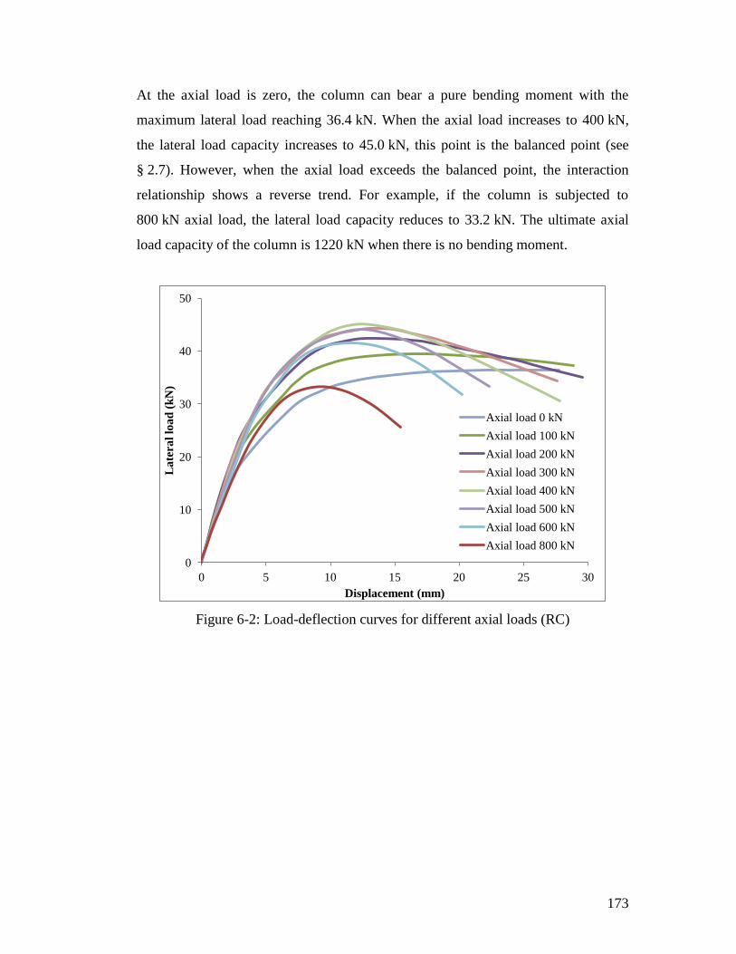
173

At the axial load is zero, the column can bear a pure bending moment with the

maximum lateral load reaching 36.4 kN. When the axial load increases to 400 kN,

the lateral load capacity increases to 45.0 kN, this point is the balanced point (see

§ 2.7). However, when the axial load exceeds the balanced point, the interaction

relationship shows a reverse trend. For example, if the column is subjected to

800 kN axial load, the lateral load capacity reduces to 33.2 kN. The ultimate axial

load capacity of the column is 1220 kN when there is no bending moment.

Figure 6-2: Load-deflection curves for different axial loads (RC)

0

10

20

30

40

50

0 5 10 15 20 25 30

La

tera

l lo

ad

(k

N)

Displacement (mm)

Axial load 0 kN

Axial load 100 kN

Axial load 200 kN

Axial load 300 kN

Axial load 400 kN

Axial load 500 kN

Axial load 600 kN

Axial load 800 kN

174

Figure 6-3: Interaction diagram for RC

Similar structural behaviour is found in the numerical simulations of FC2, FC4, in

respect to axial load against lateral load curves, as shown in Figure 6-4 (for details

see Appendix H).

At zero axial load, the lateral load capacity of FC2 is 25.6 kN, and FC4 is 41%

greater than FC2 (36.2 kN), as presented in Table 6-2.

At the balanced point, the lateral load capacities of FC2 and FC4 rise to 45.8 kN and

50.8 kN respectively; FC4 being approximately 11% higher than FC2.

When only the axial loads are applied to FC2 and FC4, without any bending moment,

the maximum axial load capacities reach 1523 kN and 1605 kN respectively. These

results show that the higher the amount of welded mesh the greater the lateral load

that can be resisted.

0

200

400

600

800

1000

1200

1400

0 10 20 30 40 50

Axia

l lo

ad

(k

N)

Lateral load (kN)

RC

175

Figure 6-4: Interaction diagram from ABAQUS simulation for FC2 and FC4

Table 6-2: Result of maximum lateral loads for different axial loads for FC2 and

FC4

Axial load (kN) Lateral load (kN) Difference

(%) FC2 FC4

0 25.2 35.6 41%

100 33.7 40.4 20%

200 37.9 44.1 16%

400 42.5 48.9 15%

600 45.8 50.3 10%

800 45.6 50.8 11%

1000 41.0 46.9 15%

1200 30.0 37.9 26%

1523 0

1605 0

0

200

400

600

800

1000

1200

1400

1600

1800

0 10 20 30 40 50 60

Axia

l lo

ad

(k

N)

Lateral load (kN)

FC2

FC4

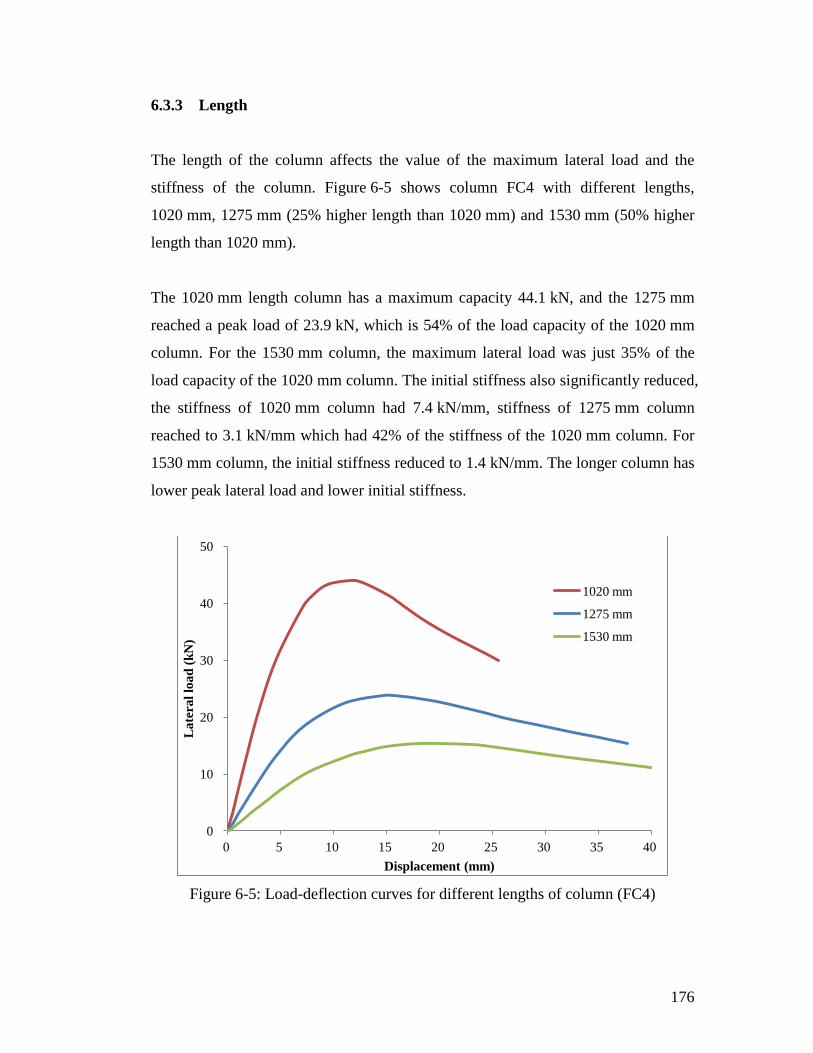
176

6.3.3 Length

The length of the column affects the value of the maximum lateral load and the

stiffness of the column. Figure 6-5 shows column FC4 with different lengths,

1020 mm, 1275 mm (25% higher length than 1020 mm) and 1530 mm (50% higher

length than 1020 mm).

The 1020 mm length column has a maximum capacity 44.1 kN, and the 1275 mm

reached a peak load of 23.9 kN, which is 54% of the load capacity of the 1020 mm

column. For the 1530 mm column, the maximum lateral load was just 35% of the

load capacity of the 1020 mm column. The initial stiffness also significantly reduced,

the stiffness of 1020 mm column had 7.4 kN/mm, stiffness of 1275 mm column

reached to 3.1 kN/mm which had 42% of the stiffness of the 1020 mm column. For

1530 mm column, the initial stiffness reduced to 1.4 kN/mm. The longer column has

lower peak lateral load and lower initial stiffness.

Figure 6-5: Load-deflection curves for different lengths of column (FC4)

0

10

20

30

40

50

0 5 10 15 20 25 30 35 40

La

tera

l lo

ad

(k

N)

Displacement (mm)

1020 mm

1275 mm

1530 mm

177

Table 6-3: Result of lateral load with varying column lengths (FC4)

Length of column

(mm)

Lateral load Stiffness

Value

(kN)

Degradation

(%)

Value

(kN/mm)

Degradation

(%)

1020 44.1

7.4

1275 23.9 54% 3.1 42%

1530 15.3 35% 1.4 19%

6.4 Concrete strength

In this section, three concrete compressive strengths are used, which are 30, 40 and

50 MPa (C30, C40 and C50) based on the Eurocode 2 (CEN, 2004a) concrete

material model (see § 5.3.2.1). The corresponding results are shown in Figure 6-6.

These results illustrate that the maximum lateral load capacity can be increased by

increasing the strength of the concrete. As shown in Figure 6-6, the lateral load

capacity of the column increases from 38.3 kN to 46.8 kN as the concrete

compressive strength is increased from C30 to C50. In addition, the initial stiffness

of the column can be increased when the concrete compressive strength arises.

Figure 6-6: Load-deflection curves for different concrete strengths (RC)

0

10

20

30

40

50

0 5 10 15 20 25 30

La

tera

l lo

ad

(k

N)

Displacement (mm)

C30

C38 (cyclinder test)

C40

C50

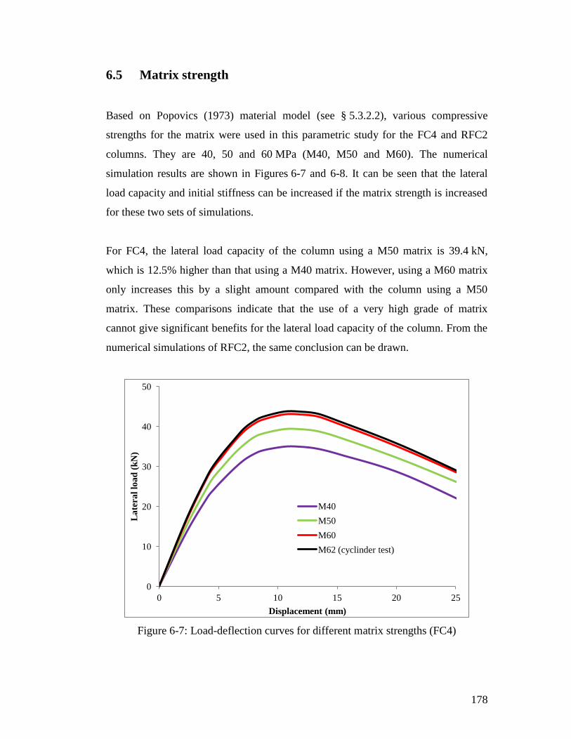
178

6.5 Matrix strength

Based on Popovics (1973) material model (see § 5.3.2.2), various compressive

strengths for the matrix were used in this parametric study for the FC4 and RFC2

columns. They are 40, 50 and 60 MPa (M40, M50 and M60). The numerical

simulation results are shown in Figures 6-7 and 6-8. It can be seen that the lateral

load capacity and initial stiffness can be increased if the matrix strength is increased

for these two sets of simulations.

For FC4, the lateral load capacity of the column using a M50 matrix is 39.4 kN,

which is 12.5% higher than that using a M40 matrix. However, using a M60 matrix

only increases this by a slight amount compared with the column using a M50

matrix. These comparisons indicate that the use of a very high grade of matrix

cannot give significant benefits for the lateral load capacity of the column. From the

numerical simulations of RFC2, the same conclusion can be drawn.

Figure 6-7: Load-deflection curves for different matrix strengths (FC4)

0

10

20

30

40

50

0 5 10 15 20 25

La

tera

l lo

ad

(k

N)

Displacement (mm)

M40

M50

M60

M62 (cyclinder test)

179

Figure 6-8: Load-deflection curves for different matrix strengths (RFC2)

6.6 Main reinforcing bar

The properties of the reinforcing bars are parameters that may drastically affect the

structural behaviour of the column. This section will investigate the effect of

reinforcing bars in terms of strength, diameter and number. Only RC column is used

to examine the main effect of the reinforcing bars.

6.6.1 Strength

Figure 6-9 shows that the lateral load capacity of the RC column increases

proportionally with the increasing strength of the steel bar. However, the initial

stiffness of the column remains unchanged, because the Young’s Modulus of the

steel bar whatever S275, S355, S480 and S525 have similar value (CEN, 2004a).

0

10

20

30

40

50

60

70

0 5 10 15 20 25 30 35

La

tera

l lo

ad

(k

N)

Displacement (mm)

M40

M50

M60

M62 (cyclinder test)

180

Figure 6-9: Load-deflection curves for different steel bar strengths (RC)

6.6.2 Diameter and number of bars

If the diameter of steel bar is enlarged, the lateral load capacity arises significantly

as shown in Figure 6-10. For example, the lateral load capacity of the column is

increased by 42% by using the steel bars having 905 mm2 cross-section area

compared with 452 mm2. The reason is the increased diameter of the steel bar can

strengthen both tension and compression resistances. Therefore, the bending

moment capacity of the column is increased.

0

10

20

30

40

50

0 5 10 15 20 25 30

La

tera

l lo

ad

(k

N)

Displacement (mm)

S275

S355

S480 (tested)

S525

181

Figure 6-10: Load-deflection curves for different cross-section areas of steel bars

(RC)

Compared with the original RC column (four steel bars at corner, detail in

Figure 3-9), there are eight steel bars which are embedded in the reinforcement

concrete for the modified column as shown in Figure 6-11 (four extra bars added).

Number 1, 2, 3 and 4 bars are original arrangement, Number 5, 6, 7 and 8 bars are

located at the middle point of each side. However, the total area (905 mm2) of steel

bars in the two columns is the same. Figure 6-12 shows the lateral load-deflection

curves for 4 bars column and 8 bars column, which the 4 bars gave a higher lateral

load capacity. The 4 bars column had peak lateral load capacity of 59.5 kN, which is

11% higher than the column using 8 bars arrangement (52.8 kN for 8 bars).

The reason is that bars 6 and 7, which are located at the neutral axial in the modified

RC column, cannot provide any bending moment resistance. Therefore, the column

using the 8 bars arrangement uses less steel for bending moment resistance.

0

10

20

30

40

50

60

0 5 10 15 20 25 30

La

tera

l lo

ad

(k

N)

Displacement (mm)

Total steel area 452 mm²



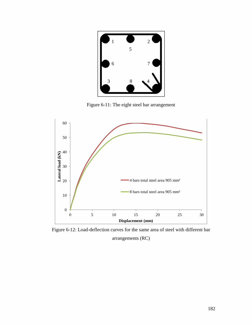
182

Figure 6-11: The eight steel bar arrangement

Figure 6-12: Load-deflection curves for the same area of steel with different bar

arrangements (RC)

0

10

20

30

40

50

60

0 5 10 15 20 25 30

La

tera

l lo

ad

(k

N)

Displacement (mm)

4 bars total steel area 905 mm²

8 bars total steel area 905 mm²

1 2

6 7

3 8 4

5

183

6.7 Stirrups

This section analyzes the influence of the stirrups on the structural behaviour of the

column. Two aspects of the stirrups are considered: strength and size.

6.7.1 Strength

The stirrups only play a confinement role in reinforced concrete. Hence, Figure 6-13

shows that varying the strength of the stirrup cannot change the column relationship

between lateral load and deflection.

Figure 6-13: Load-deflection curves for different stirrup strengths (RC)

0

10

20

30

40

50

0 5 10 15 20 25 30

La

tera

l lo

ad

(k

N)

Displacement (mm)

Stirrup S275

Stirrup S355

Stirrup S525

Stirrup S600 (test used)

184

6.7.2 Size

Again, Figure 6-14 shows that the size of the stirrups has no effect on the column

structural behaviour in terms of the load-deflection relationship. This further

demonstrates the confinement role of the stirrups.

Figure 6-14: Load-deflection curves for different cross-section areas of stirrups (RC)

Whatever varying with the grade of stirrups and cross-section of stirrups, the value

of lateral load had not significant change. The main contribution of the stirrups is to

provided confined effect to the column, however, the stirrups has negligible effect

on the bending moment capacity of the column.

0

10

20

30

40

0 5 10 15 20 25 30

La

tera

l lo

ad

(k

N)

Displacement (mm)

Stirrup 7.07 mm² (used)

Stirrup 14.1 mm²

Stirrup 28.3 mm²

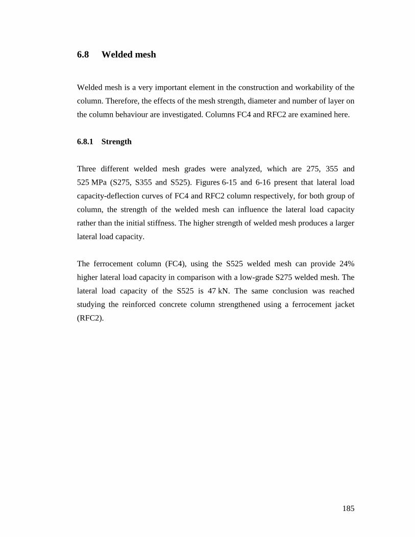
185

6.8 Welded mesh

Welded mesh is a very important element in the construction and workability of the

column. Therefore, the effects of the mesh strength, diameter and number of layer on

the column behaviour are investigated. Columns FC4 and RFC2 are examined here.

6.8.1 Strength

Three different welded mesh grades were analyzed, which are 275, 355 and

525 MPa (S275, S355 and S525). Figures 6-15 and 6-16 present that lateral load

capacity-deflection curves of FC4 and RFC2 column respectively, for both group of

column, the strength of the welded mesh can influence the lateral load capacity

rather than the initial stiffness. The higher strength of welded mesh produces a larger

lateral load capacity.

The ferrocement column (FC4), using the S525 welded mesh can provide 24%

higher lateral load capacity in comparison with a low-grade S275 welded mesh. The

lateral load capacity of the S525 is 47 kN. The same conclusion was reached

studying the reinforced concrete column strengthened using a ferrocement jacket

(RFC2).

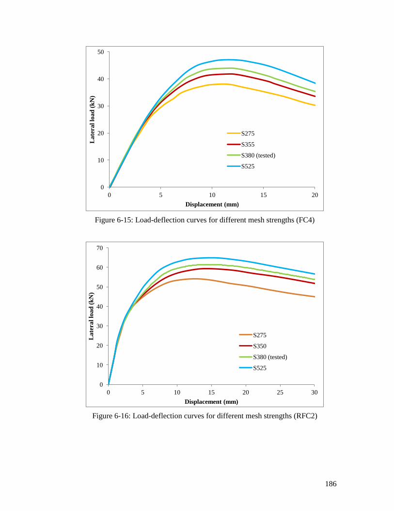
186

Figure 6-15: Load-deflection curves for different mesh strengths (FC4)

Figure 6-16: Load-deflection curves for different mesh strengths (RFC2)

0

10

20

30

40

50

0 5 10 15 20

La

tera

l lo

ad

(k

N)

Displacement (mm)

S275

S355

S380 (tested)

S525

0

10

20

30

40

50

60

70

0 5 10 15 20 25 30

La

tera

l lo

ad

(k

N)

Displacement (mm)

S275

S350

S380 (tested)

S525

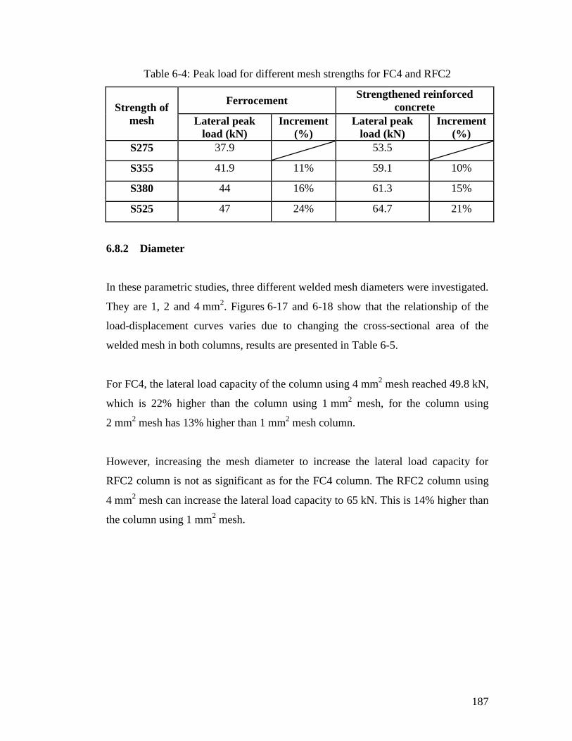
187

Table 6-4: Peak load for different mesh strengths for FC4 and RFC2

Strength of

mesh

Ferrocement Strengthened reinforced

concrete

Lateral peak

load (kN)

Increment

(%)

Lateral peak

load (kN)

Increment

(%)

S275 37.9

53.5

S355 41.9 11% 59.1 10%

S380 44 16% 61.3 15%

S525 47 24% 64.7 21%

6.8.2 Diameter

In these parametric studies, three different welded mesh diameters were investigated.

They are 1, 2 and 4 mm2. Figures 6-17 and 6-18 show that the relationship of the

load-displacement curves varies due to changing the cross-sectional area of the

welded mesh in both columns, results are presented in Table 6-5.

For FC4, the lateral load capacity of the column using 4 mm2 mesh reached 49.8 kN,

which is 22% higher than the column using 1 mm2 mesh, for the column using

2 mm2 mesh has 13% higher than 1 mm

2 mesh column.

However, increasing the mesh diameter to increase the lateral load capacity for

RFC2 column is not as significant as for the FC4 column. The RFC2 column using

4 mm2 mesh can increase the lateral load capacity to 65 kN. This is 14% higher than

the column using 1 mm2 mesh.

188

Figure 6-17: Load-deflection curves for different mesh sizes (FC4)

Figure 6-18: Load-deflection curves for different mesh sizes (RFC2)

0

10

20

30

40

50

60

0 5 10 15 20

La

tera

l lo

ad

(k

N)

Displacement (mm)

Mesh 1 mm²

Mesh 2 mm²

Mesh 4 mm²

0

10

20

30

40

50

60

70

0 5 10 15 20 25 30 35

La

tera

l lo

ad

(k

N)

Displacement (mm)

Mesh 1 mm²

Mesh 2 mm²

Mesh 4 mm²

189

Table 6-5: Peak load for various cross-sectional areas of mesh for FC2 and RFC2

Cross-section of

mesh (mm2)

FC4 RFC2

Lateral peak

load (kN)

Increment

(%)

Lateral peak

load (kN)

Increment

(%)

1 39.8

56.6

2 44.9 13% 61.5 9%

4 49.8 22% 65 14%

6.8.3 Number of layers

The load-displacement curves for FC columns and RFC with varying numbers of

layers mesh are shown in Figures 6-19 and 6-20, respectively. Obviously, increasing

the number of layers for both group arise the maximum lateral load capacity. The

stiffness of the ferrocement also increased as the number of layer increased, but for

RFC this is not distinct.

Table 6-6 shows the peak lateral load for increasing numbers of mesh layers and the

percentage load increase both for FC and RFC. The one-layer mesh FC (FC1) had a

peak load of 37 kN. For the two-layer mesh column, the lateral load rose to 40.8 kN,

which is 10% higher; and for FC5 it reached 46.8 kN (26% higher).

For RFC, the one-layer mesh column had a peak lateral load of 57.6 kN. For the

two-layers mesh, it was 61.8 kN, which is 7% greater, and for the four-layer mesh

(RFC4) it increased to 72.7 kN (26% greater).

The higher amount of mesh can strengthen both tension and compression resistances,

so the bending moment capacity of the column is increased.

190

Figure 6-19: Load-deflection curves for different numbers of layers of mesh (FC)

Figure 6-20: Load-deflection curves for different numbers of layers of mesh (RFC)

0

10

20

30

40

50

0 5 10 15 20

La

tera

l lo

ad

(k

N)

Displacement (mm)

1 layer

2 layers

3 layers

4 layers

5 layers

0

10

20

30

40

50

60

70

80

0 5 10 15 20 25 30 35

La

tera

l lo

ad

(k

N)

Displacement (mm)

1 layer

2 layers

3 laters

4 layers

191

Table 6-6: Peak load for FC and RFC with different numbers of mesh layer

Number of

layers

Ferrocement Strengthened reinforced

concrete

Lateral peak

load (kN)

Increment

(%)

Lateral peak

load (kN)

Increment

(%)

1 37

57.6

2 40.8 10% 61.8 7%

3 43.1 16% 68.5 19%

4 44.9 21% 72.7 26%

5 46.8 26%

6.9 Summary

In this chapter details of the parametric studies results have been presented. The

following points are emphasized:

Several parameters were examined using the ABAQUS simulation. These

include end conditions, axial load, length of column, properties of the material

and diameter of the reinforcement.

The end condition and axial load have a significant effect on the peak lateral

load. It has the same initial stiffness as the experiment bending-shear effect

(detail in Chapter 4 and § 6.3.1).

With increasing grade of concrete or matrix, the peak load increases.

For the stirrups, changes in the strength or cross-section area of the stirrup had

negligible effect on the peak load capacity of the column.

The interaction diagrams for ferrocement are similar; with FC4 having 10%

greater lateral load than FC2 at the balanced point.

192

CHAPTER 7 Design guidelines

7.1 Introduction

The current design of ferrocement structures is usually based on the

recommendations of Naaman (2000), IFS code (IFS, 2001) and ACI 549 (ACI,

1997b); however, design guidelines for ferrocement columns and reinforced

concrete columns strengthened using ferrocement are not yet available. In this

chapter, interaction diagrams for both FC and RFC columns are presented and

design guidelines for columns are given.

For the design guidelines, the matrix properties are based on ACI 318 (ACI, 2008)

and a simplification of Popovics (1973) model is used, as shown in the following

section.

7.2 Material property

7.2.1 Welded mesh property

The property of welded mesh is assumed as a bi-linear (idealization) curve for the

design guide, as shown in Figure 7-1. The first stage of the idealization curve is from

0 to the yield point ( ), the slope of this stage is the same as the Young’s

Modulus for the experimental test curve (175000 N/mm2). The second stage is after

the yield point.

193

Figure 7-1: Ideal mesh bi-linear curve (S380)

The Young’s Modulus of the mesh ( ) for S380 (used in experimental test) is

175000 N/mm2, and slope for second stage ( ) is calculated as:

Eq 7-1

Selecting a point where stress ( ) at 420 N/mm2 and strain ( ) is 0.05, then

Eq 7-2

0

50

100

150

200

250

300

350

400

450

500

0.00 0.01 0.02 0.03 0.04 0.05 0.06

Str

ess

(MP

a)

Strain

Experimental test

Idealization

y=0.0022

σy=380 MPa

Emesh=175000 MPa

Emesh.u=836 MPa

194

7.2.2 Matrix property

The property of the matrix is based on ACI 318 (ACI, 2008) and uses a

simplification of Popovics (1973) model, and is shown in Figure 7-2. This curve was

obtained in tests in the laboratory. This matrix was used in the FC2, FC4, RFC2 and

RFC3 columns. The strength of this matrix is 62 N/mm2 (called M62).

The “red” colour in Figure 7-2 presents Popovics model. This model is derived from

experimental data; the details of which are shown in § 5.3.2.2. The maximum matrix

compressive strain is usually between 0.003 and 0.004 (ACI, 2008). For M62, a

strain of 0.004 was chosen as the ultimate strain.

The “blue” colour is a rectangular section which is recommended by ACI 318 (ACI,

2008). The stress-block having 0.85 and strain is , where is a factor of

the stress-block length related to the ultimate strain (see Figures 7-2 and 7-3).

The value of varies with the strength of the matrix and can be calculated using

Eq 7-3, which is given by ACI 318 (ACI, 2008)

Eq 7-3

So for M62, the value of

, then .

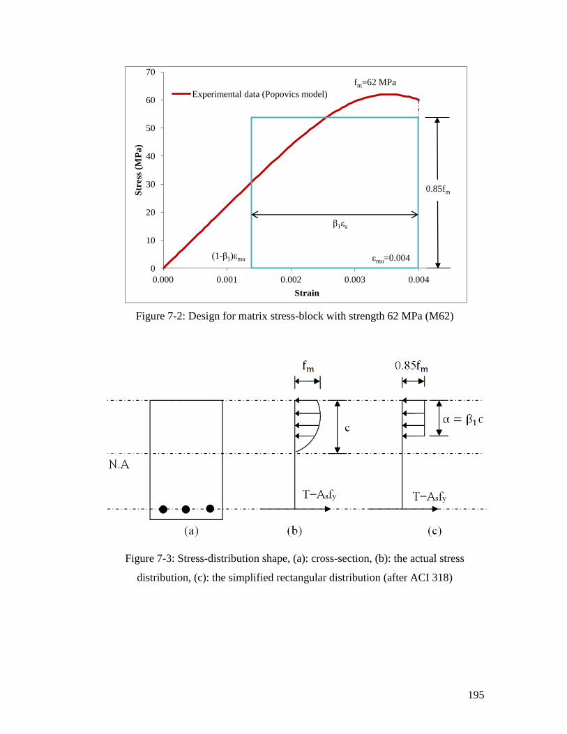
195

Figure 7-2: Design for matrix stress-block with strength 62 MPa (M62)

Figure 7-3: Stress-distribution shape, (a): cross-section, (b): the actual stress

distribution, (c): the simplified rectangular distribution (after ACI 318)

0

10

20

30

40

50

60

70

0.000 0.001 0.002 0.003 0.004

Str

ess

(MP

a)

Strain

Experimental data (Popovics model)

fm=62 MPa

mu=0.004 (1- 1) mu

0.85fm

1 u

196

Where:


Distance from extreme compression to neutral axis (N.A)


Factor relating depth of equivalent rectangular compressive stress

block to neutral axis (N.A) depth

For design, the tensile strength of the matrix is ignored.

7.3 Theoretical interaction diagrams and FEM results

7.3.1 The simplified strain and stress distribution diagram of FC4

To simplify the problem, assume that the welded mesh is uniformly distributed and

the number of layers are merged as one, as shown in Figure 7-4. The next section

gives an example (FC4, 150 150 mm) to describe and calculate the important

points in the interaction diagram.

Firstly, the author assumed that the welded mesh in the ferrocement column is

uniformly distributed with uniform cover thickness (minimum 3 mm) and spacing of

12.6 mm (the welded mesh opening is 12.6 mm). Calculate the number of strands for

each side.

Therefore, each side of the section has 12 strands and the cover is 5.5 mm. As the

FC4 section is uniform and symmetrical, so the central axis (C.A) is through the

middle of the section. The distance “c” (see Figure 7-3) is from the extreme

compression surface to the position of the neutral axis (N.A).

197

As force equilibrium, the compressive and tensile forces must be balanced, which

the compressive force include matrix and compressive mesh ( ), and the

tensile force from tensile mesh . Notice that the force balance should consider

the value of P, where P is the axial load on the section (see Figure 7-5), and Eq 7-4

shows the theoretical formula.

Eq 7-4

Where:

Axial force

Force of matrix under compression

Total force of welded mesh under compression

Total force of welded mesh under tension

i The letter “i” is number of meshes level

Define the compressive forces to be positive ( and ) and tensile forces to be

negative ( ). For each part of the Eq 7-4 is shown below:

The value of is calculated in Eq 7-5, and displayed in § 7.2.2.

) ) Eq 7-5

The value of is the sum of the forces at all welded mesh levels in compression,

and is the sum of forces at all mesh levels in tension. For accuracy, the forces at

the mesh levels should be calculated individually. On failure of the section, the peak

strain of the matrix ( ) is 0.004, so the strain of mesh layer is calculated as shown

in Eq 7-6.

)

Eq 7-6

The stress for each mesh level can be found using Eq 7-2, then the forces at the mesh

levels can be determined, are shown in Eq 7-7 and Eq 7-8. When the value of is

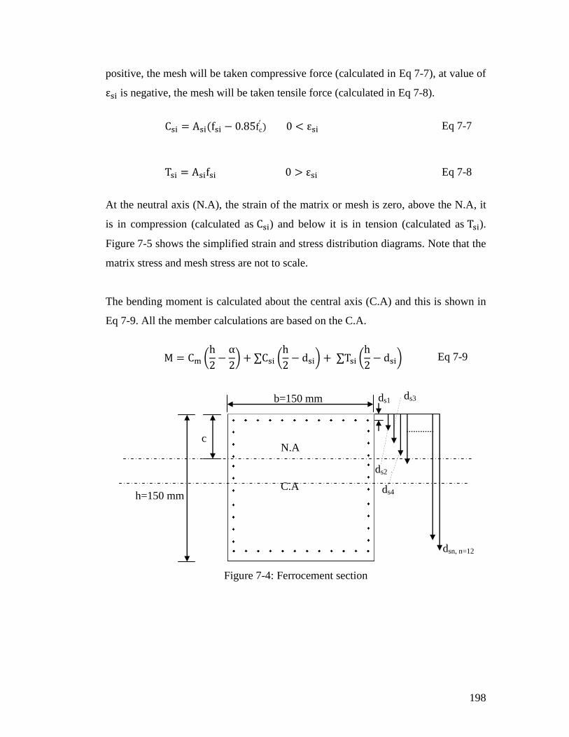
198

positive, the mesh will be taken compressive force (calculated in Eq 7-7), at value of

is negative, the mesh will be taken tensile force (calculated in Eq 7-8).

) Eq 7-7

Eq 7-8

At the neutral axis (N.A), the strain of the matrix or mesh is zero, above the N.A, it

is in compression (calculated as ) and below it is in tension (calculated as ).

Figure 7-5 shows the simplified strain and stress distribution diagrams. Note that the

matrix stress and mesh stress are not to scale.

The bending moment is calculated about the central axis (C.A) and this is shown in

Eq 7-9. All the member calculations are based on the C.A.

Eq 7-9

Figure 7-4: Ferrocement section

b=150 mm ds1

ds2

ds3

ds4

dsn, n=12

h=150 mm

N.A

C.A

c

199

Figure 7-5: The simplified strain and stress distribution diagram

Note： the matrix stress and mesh stress are not to scale

7.3.2 Interaction diagram (P-M) for the matrix

Figure 7-6 shows the interaction diagram (P-M), through the different values of axial

load and positions of the N.A There are four important situations: (i) point a, pure

bending moment, (ii) point b, balance position, (iii) point bc, zero strain in the

tension mesh, (iv) point c, pure axial load. A detailed description is provided below.

C.A

N.A

0.004 0.85

c

=

M

P

0.0022

(a): Strain distribution (b): Stress distribution (c): Force and Moment

σ =380 N/mm2

Yield stress

Bi-linear stress

distribution

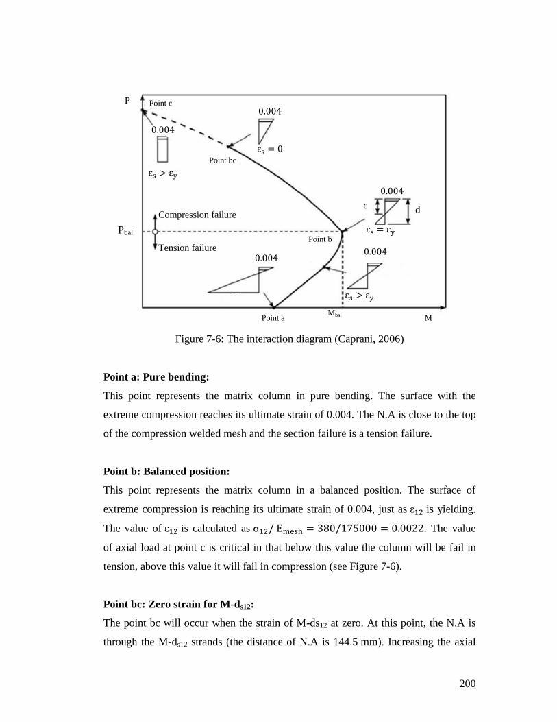
200

Figure 7-6: The interaction diagram (Caprani, 2006)

Point a: Pure bending:

This point represents the matrix column in pure bending. The surface with the

extreme compression reaches its ultimate strain of 0.004. The N.A is close to the top

of the compression welded mesh and the section failure is a tension failure.

Point b: Balanced position:

This point represents the matrix column in a balanced position. The surface of

extreme compression is reaching its ultimate strain of 0.004, just as is yielding.

The value of is calculated as . The value

of axial load at point c is critical in that below this value the column will be fail in

tension, above this value it will fail in compression (see Figure 7-6).

Point bc: Zero strain for M-ds12:

The point bc will occur when the strain of M-ds12 at zero. At this point, the N.A is

through the M-ds12 strands (the distance of N.A is 144.5 mm). Increasing the axial

Pbal

Compression failure

Tension failure

P

Mbal M Point a

Point b

Point bc

Point c

201

load forms the balanced position (Point b shows in Figure 7-6), then the N.A moves

to the tensile zone, until it reached M-ds12. All the mesh takes a compressive force

(not including M-ds12, which takes no force).

Point c: Pure axial load

This point represents the matrix column under pure axial load. All the surfaces are

taken equally in compression. M is zero and the N.A is at infinity.

7.4 Example calculation using FC4

7.4.1 Information required

The mesh arrangement is exactly as in Figure 7-4. Before the calculation, the

dimensions and properties will be presented. Table 7-1 shows the dimension of the

matrix and welded mesh section. Table 7-2 shows the properties of the matrix and

mesh. Table 7-3 shows the position of each mesh level.

Dimensions:

Table 7-1: Dimensions of the matrix and the welded mesh

Matrix

h (mm) 150

b (mm) 150

Ag (mm2) 22500

Welded mesh

Diameter (mm) 1.6

Opening (mm) 12.6

As for single wire (mm2) 2.01

As1 and As12 (mm2) 2.01 4 12=96.5

As2, As3, ......, As11 (mm2) 2.01 4 2=16.1

202

Properties:

Table 7-2: The properties of matrix and welded mesh

Matrix

(N/mm2) 62

(N/mm2) 21700

0.004

0.65

Welded mesh

(N/mm2) 380

(N/mm2) 175000

380/175000=0.0022

(N/mm2) 836

Arrangement:

Table 7-3: The position of each mesh level, dsi

Level of mesh Each mesh layer

area As (mm2)

Distance from extreme

compression dsi (mm)

1 96.5 5.5

2 16.1 18.1

3 16.1 30.8

4 16.1 43.4

5 16.1 56.0

6 16.1 68.7

7 16.1 81.3

8 16.1 94.0

9 16.1 106.6

10 16.1 119.2

11 16.1 131.9

12 96.5 144.5

203

7.4.2 Point a: Pure moment

In the detailed calculations that follow, the convention that is adopted is that

compression is positive and tension is negative. A trial and error method is used in

this section, to solve the values of c (position of N.A) at different points. This

method uses “EXCEL” and is presented in Tables 7-4 and 7-5.

Input a value of c, the mesh strain, mesh stress, mesh force, mesh moment, matrix

force and moment for each member to be calculated using the load equilibrium and

moment equilibrium equations (Eq 7-4 and Eq 7-9). Figure 7-7 shows the strain

diagram of the N.A for pure moment.

For pure moment, the value of the axial load (P) is zero, as shown:

Eq 7-10

For the trial and error method, set two basic values of “c”, say 5.5 mm and 75 mm,

when the N.A passes through M-ds1 and the central axis. After calculation, the

position of N.A (c) is found to be 12.7 mm for a total axial load (P) of zero.

Table 7-4 presents the results for the mesh strain, stress, force and moment. The

mesh strain variation from positive 0.0023 (M-ds1) to negative 0.04312 (M-ds12), is

calculated as being linear (see Figure 7-5), and the extreme compression matrix

surface is 0.004.

The mesh strain for each level of mesh is calculated using Eq 7-2. This equation is a

bi-linear curve for mesh strength (see Figure 7-1).

The mesh force is the mesh stress times the cross-section area of each mesh level.

M-ds12 has taken the highest force which is 39.9 kN. The calculation requires the

compressive strength (always positive) and the tensile strength (always

negative).

204

The mesh moment, Eq 7-9, is calculated as:

Compressive mesh moment:

Eq 7-11

Tensile mesh moment:

Eq 7-12

The value of ) will be positive above the central axis (C.A.), and negative

below it. So the mesh moment of M-ds1 is 2.55 kNm (only this mesh level has a

positive mesh force, which the force is 36.7 kN). The second level mesh has a tensile

force (negative 4.82 kN), so the resulting moment is -0.27 kNm. Then, the values of

the moment in the mesh are all negative above the C.A.

Below the C.A. the value of ) is negative, so the tensile force in the mesh

is negative, but the resulting mesh moment becomes positive (negative times

negative). The highest value of the moment is M-ds12, 2.77 kNm, and the lowest

value, which is close to the C.A. is 0.04 kNm, for M-ds6 is negative value and M-ds7

has positive value.

Table 7-4: Force and moment for meshes for the pure moment (c=12.7 mm)

Mesh

name

Mesh strain

(εsi)

Mesh stress fsi

(MPa)

Mesh force

(kN)

Mesh moment

(kNm)

M-ds1 0.0023 380.1 36.7 2.55

M-ds2 -0.0017 -291.8 -4.82 -0.27

M-ds3 -0.0056 -382.9 -6.16 -0.27

M-ds4 -0.0096 -386.2 -6.21 -0.20

M-ds5 -0.0135 -389.5 -6.27 -0.12

M-ds6 -0.0175 -392.8 -6.32 -0.04

M-ds7 -0.0214 -396.1 -6.37 0.04

M-ds8 -0.0254 -399.4 -6.43 0.12

M-ds9 -0.0293 -402.7 -6.48 0.20

M-ds10 -0.0333 -406.0 -6.53 0.29

M-ds11 -0.0372 -409.3 -6.59 0.37

M-ds12 -0.0412 -412.6 -39.9 2.77

205

Table 7-5 shows the total mesh force and mesh moment. The total force is zero,

which compressive matrix is 65.3 kN, compressive mesh is 36.7 kN and tensile

mesh force is negative 102 kN. The moment of the compressive matrix is 4.62 kNm,

and the moment of the compressive mesh is 2.55 kNm. The rest of the mesh takes a

tensile force, so the moment is 2.90 kNm. The total moment is the sum of the three

parts, which gives 10.1 kNm (which calculated as 4.62+2.55+2.90=10.1 kNm).

Table 7-5: Results for total axial load and moment of meshes for the pure moment

Description Force

(kN) Moment (kNm)

Compressive matrix 65.3

4.62

Compressive meshes 36.7

2.55

Tensile meshes -102

2.90

Total P 0 M 10.1

Figure 7-7: Strain diagram of the N.A for a pure moment

N.A

0.0412

0.004

0.0023

c= 12.7 mm

C.A

206

7.4.3 Point b: Strength at the balanced condition

Point b is when the compressive matrix reaches its ultimate strain (0.004) and the

tension reinforcement, M-ds12, yields (0.0022) simultaneously. The load equilibrium

is based on Eq 7-4. As the axial load increases, the compression matrix and

reinforcing forces are increased, and the N.A moves in the tensile direction.

Between the pure bending and the balanced position conditions, the strain of the

tensile mesh (M-ds12) is greater than the mesh at yielding, which is fail as a tensile

failure. After the balanced position the column will fail as a compression failure.

Again, the value of mesh strain, stress, force and moment is calculated using the

same method (trial and error method). The position of N.A (c) is equal 93.7 mm.

Tables 7-6 and 7-5 show the results.

Table 7-6: Force and moment of meshes at the balanced condition (c=93.7 mm)

Mesh

name

Mesh strain

(εsi)

Mesh stress fsi

(MPa)

Mesh force

(kN)

Mesh moment

(kNm)

M-ds1 0.0038 381.3 36.8 2.56

M-ds2 0.0032 380.9 6.13 0.35

M-ds3 0.0027 380.4 6.12 0.27

M-ds4 0.0021 375.7 6.04 0.19

M-ds5 0.0016 281.3 4.52 0.09

M-ds6 0.0011 186.9 3.01 0.02

M-ds7 0.0005 92.5 1.49 -0.01

M-ds8 0.0000 -1.9 -0.03 0.00

M-ds9 -0.0006 -96.3 -1.55 0.05

M-ds10 -0.0011 -190.7 -3.07 0.14

M-ds11 -0.0016 -285.1 -4.59 0.26

M-ds12 -0.0022 -379.5 -36.63 2.55

207

Table 7-7: Results of total axial load and moment of meshes at balanced condition

Description Force (kN) Moment (kNm)


21.4


3.46

Tensile meshes -45.9

2.99

Total P 499.7 M 27.9

When the N.A is at 93.7 mm, nearly two-thirds of the section from the surface, 7

level meshes (M-ds1 to M-ds7) takes compression, and M-ds1 takes 36.8 kN force. The

strain of M-ds12 is negative 0.0022 (just yielding), when it has taken 36.7 kN force in

tension.

The axial load at the balanced position is 499.7 kN. Most of the axial load is

supported by matrix compression (481.4 kN). The moment at balanced position is

27.9 kNm.

Figure 7-8: Strain diagram of the N.A at the balanced position

N.A

0.0022

0.004 0.0038

c = 93.7 mm

C.A

208

7.4.4 Point bc: M-ds12 mesh at zero tensile strain

After the axial load exceeds 499.7 kN (the load for the balanced position), the N.A

moves further towards the tension surface, and the section will fail as a compression

failure. The strain of the matrix surface reaches a peak strain before M-ds12 yields.

When the N.A moves to M-ds12, the strain of M-ds12 is zero, so no mesh takes

tension. Tables 7-8 and 7-9 show the results of the N.A at through the first level

mesh (M-ds1), the value of “c” is 144.5 mm.

Table 7-8: Force and moment of meshes at point bc (c=144.5 mm)

Mesh

name

Mesh strain

(εsi)

Mesh stress fsi

(MPa)

Mesh force

(kN)

Mesh moment

(kNm)

M-ds1 0.0038 381.4 36.81 2.56

M-ds2 0.0035 381.1 6.13 0.35

M-ds3 0.0031 380.8 6.13 0.27

M-ds4 0.0028 380.5 6.12 0.19

M-ds5 0.0024 380.2 6.12 0.12

M-ds6 0.0021 367.3 5.91 0.04

M-ds7 0.0017 306.1 4.92 -0.03

M-ds8 0.0014 244.9 3.94 -0.07

M-ds9 0.0010 183.6 2.95 -0.09

M-ds10 0.0007 122.4 1.97 -0.09

M-ds11 0.0003 61.2 0.98 -0.06

M-ds12 0 0.0 0.00 0.00

209

Table 7-9: Results of total axial load and moment of meshes at point bc

Description Force (kN) Moment (kNm)


20.8


3.18

Tensile meshes 0.00

0.00

Total P 824.5 M 24.0

The N.A moves to 144.5 mm. At this position, no-one mesh level takes a tension

force. The matrix compression supports 742.5 kN, and the value of axial load

reaches 824.5 kN. The value of total moment is 24.0 kNm. The moment of mesh is

only 3.18 kNm. Figure 7-9 shows the simplified strain diagram with the N.A at M-

ds12.

Figure 7-9: Strain diagram for the N.A at the balanced position

0

0.004 0.38

c=144.5 mm

N.A

C.A

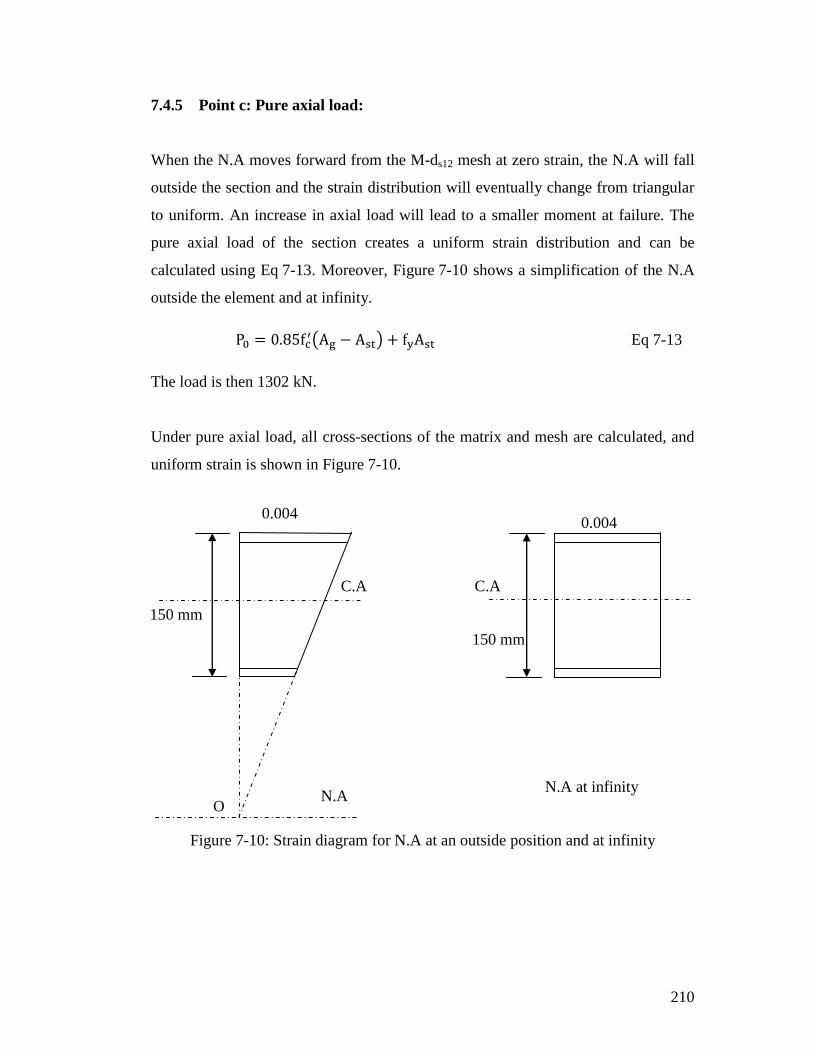
210

7.4.5 Point c: Pure axial load:

When the N.A moves forward from the M-ds12 mesh at zero strain, the N.A will fall

outside the section and the strain distribution will eventually change from triangular

to uniform. An increase in axial load will lead to a smaller moment at failure. The

pure axial load of the section creates a uniform strain distribution and can be

calculated using Eq 7-13. Moreover, Figure 7-10 shows a simplification of the N.A

outside the element and at infinity.

Eq 7-13

The load is then 1302 kN.

Under pure axial load, all cross-sections of the matrix and mesh are calculated, and

uniform strain is shown in Figure 7-10.

Figure 7-10: Strain diagram for N.A at an outside position and at infinity

C.A

0.004

150 mm

O

150 mm

N.A at infinity

0.004

N.A

C.A

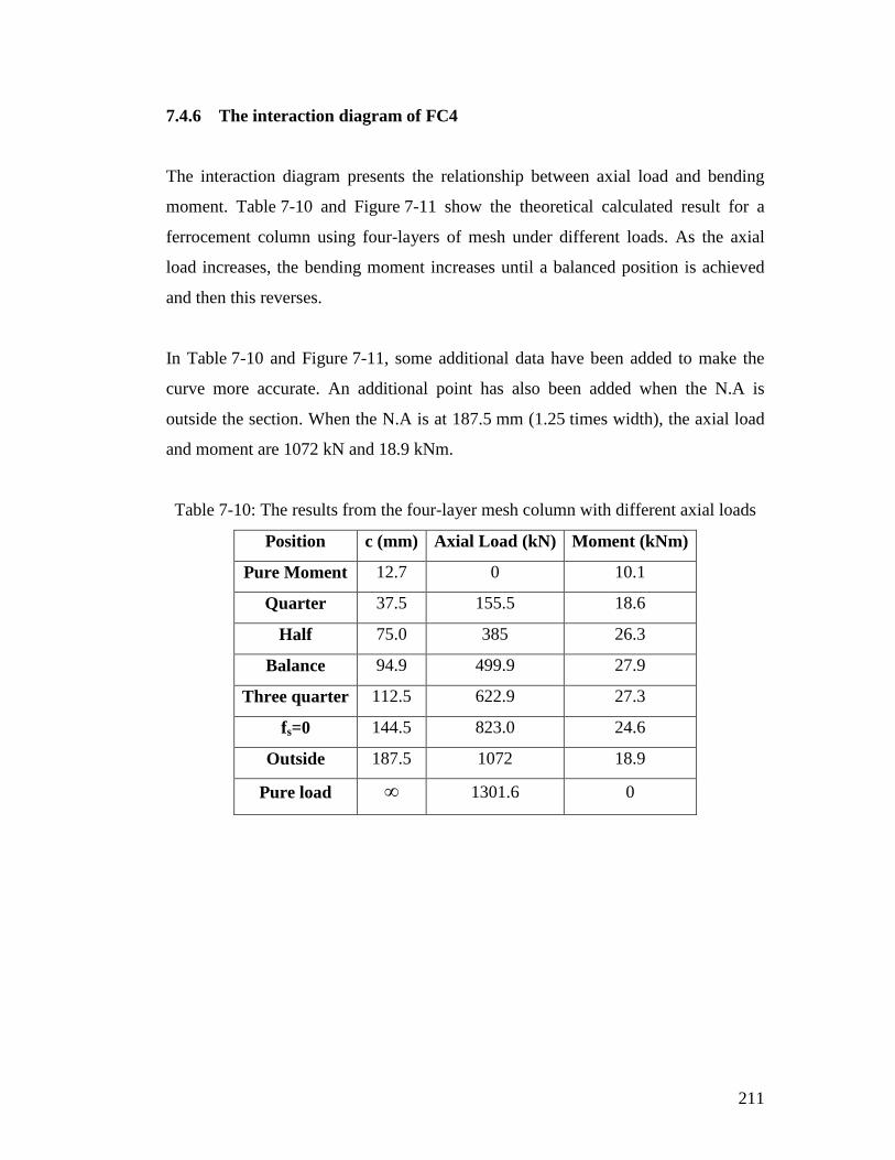
211

7.4.6 The interaction diagram of FC4

The interaction diagram presents the relationship between axial load and bending

moment. Table 7-10 and Figure 7-11 show the theoretical calculated result for a

ferrocement column using four-layers of mesh under different loads. As the axial

load increases, the bending moment increases until a balanced position is achieved

and then this reverses.

In Table 7-10 and Figure 7-11, some additional data have been added to make the

curve more accurate. An additional point has also been added when the N.A is

outside the section. When the N.A is at 187.5 mm (1.25 times width), the axial load

and moment are 1072 kN and 18.9 kNm.

Table 7-10: The results from the four-layer mesh column with different axial loads

Position c (mm) Axial Load (kN) Moment (kNm)

Pure Moment 12.7 0 10.1

Quarter 37.5 155.5 18.6

Half 75.0 385 26.3

Balance 94.9 499.9 27.9

Three quarter 112.5 622.9 27.3

fs=0 144.5 823.0 24.6

Outside 187.5 1072 18.9

Pure load ∞ 1301.6 0

212

Figure 7-11: The interaction curve for FC4 by theoretical calculation

7.5 Theoretical results

The theoretical results for the interaction diagrams for FC2, FC4, RFC2 and RFC3

are shown in Figures 7-12 and 7-13. The procedure for producing the interaction

diagrams has been demonstrated in the previous section. It clearly shows that in both

figures, theoretical results present the same trend, when the amount of mesh

increases, the axial load or the moment increase. Results are presented in Tables

7-11 and 7-12.

Pure moment condition:

From theory calculation, FC2 has a moment 5.3 kNm, and FC4 has a moment that is

90% higher than FC2, which reached 10.1 kNm. The N.A of FC2 is 8.2 mm and of

FC4 is 12.7 mm. For RFC3 at pure moment the moment is 26.3 kNm, which is 15%

higher than for RFC2.

0

200

400

600

800

1000

1200

1400

0 5 10 15 20 25 30

Axia

l lo

ad

(k

N)

Moment (kNm)

FC4 Theoretical

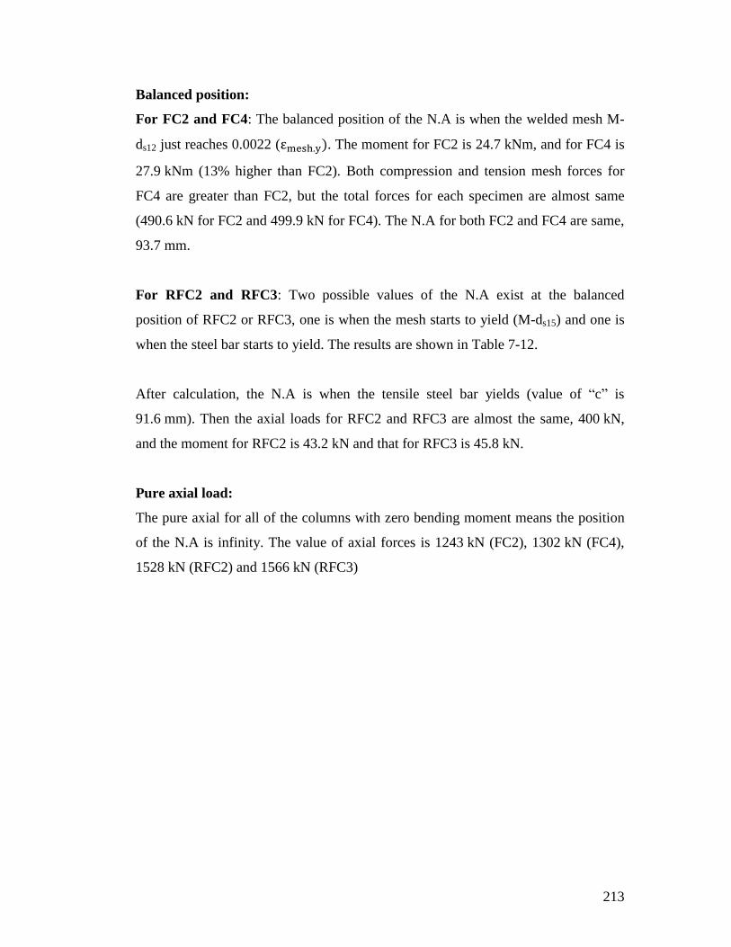
213

Balanced position:

For FC2 and FC4: The balanced position of the N.A is when the welded mesh M-

ds12 just reaches 0.0022 ( ). The moment for FC2 is 24.7 kNm, and for FC4 is

27.9 kNm (13% higher than FC2). Both compression and tension mesh forces for

FC4 are greater than FC2, but the total forces for each specimen are almost same

(490.6 kN for FC2 and 499.9 kN for FC4). The N.A for both FC2 and FC4 are same,

93.7 mm.

For RFC2 and RFC3: Two possible values of the N.A exist at the balanced

position of RFC2 or RFC3, one is when the mesh starts to yield (M-ds15) and one is

when the steel bar starts to yield. The results are shown in Table 7-12.

After calculation, the N.A is when the tensile steel bar yields (value of “c” is

91.6 mm). Then the axial loads for RFC2 and RFC3 are almost the same, 400 kN,

and the moment for RFC2 is 43.2 kN and that for RFC3 is 45.8 kN.

Pure axial load:

The pure axial for all of the columns with zero bending moment means the position

of the N.A is infinity. The value of axial forces is 1243 kN (FC2), 1302 kN (FC4),

1528 kN (RFC2) and 1566 kN (RFC3)

214

Figure 7-12: The interaction diagram for FC2 and FC4 by theoretical calculation

Figure 7-13: The interaction diagram for RFC2 and RFC3 by theoretical calculation

0

200

400

600

800

1000

1200

1400

0 5 10 15 20 25 30

Axia

l lo

ad

(k

N)

Moment (kNm)

FC2 Theoretical

FC4 Theoretical

0

200

400

600

800

1000

1200

1400

1600

1800

0 10 20 30 40 50

Axia

l lo

ad

(k

N)

Moment (kNm)

RFC2 Theoretical

RFC3 Theoretical

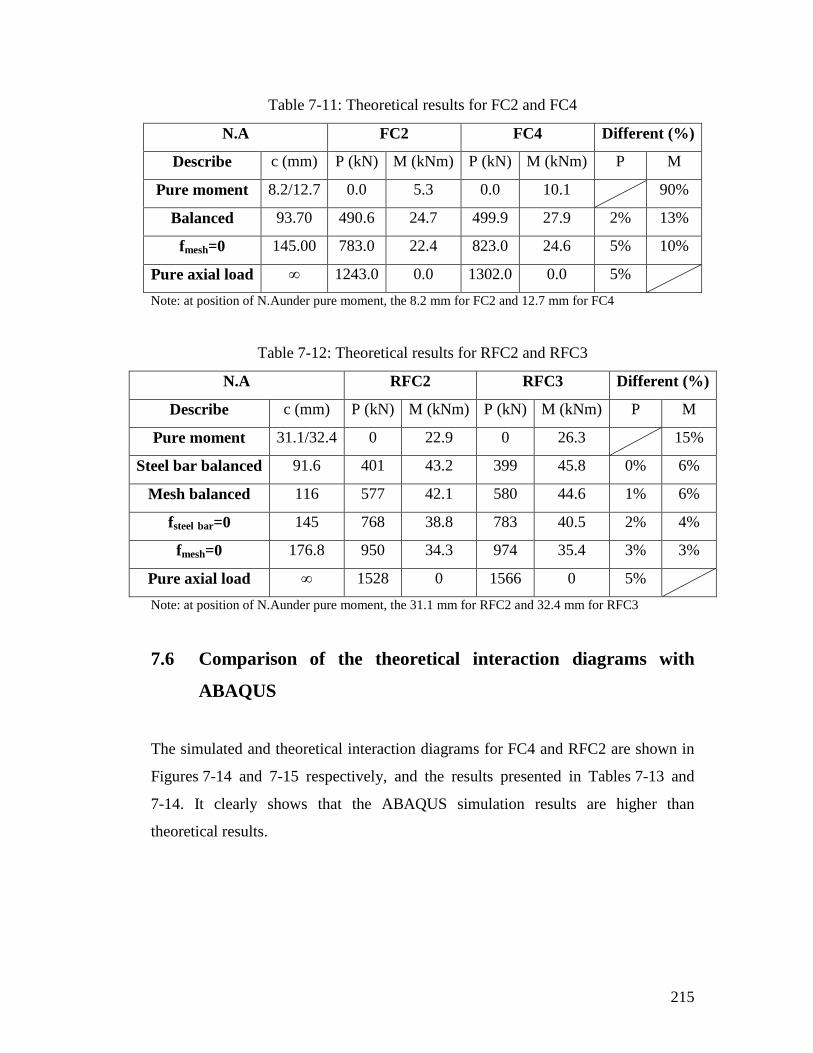
215

Table 7-11: Theoretical results for FC2 and FC4

N.A FC2 FC4 Different (%)

Describe c (mm) P (kN) M (kNm) P (kN) M (kNm) P M

Pure moment 8.2/12.7 0.0 5.3 0.0 10.1

90%

Balanced 93.70 490.6 24.7 499.9 27.9 2% 13%

fmesh=0 145.00 783.0 22.4 823.0 24.6 5% 10%

Pure axial load ∞ 1243.0 0.0 1302.0 0.0 5%

Note: at position of N.Aunder pure moment, the 8.2 mm for FC2 and 12.7 mm for FC4

Table 7-12: Theoretical results for RFC2 and RFC3

N.A RFC2 RFC3 Different (%)

Describe c (mm) P (kN) M (kNm) P (kN) M (kNm) P M

Pure moment 31.1/32.4 0 22.9 0 26.3

15%

Steel bar balanced 91.6 401 43.2 399 45.8 0% 6%

Mesh balanced 116 577 42.1 580 44.6 1% 6%

fsteel bar=0 145 768 38.8 783 40.5 2% 4%

fmesh=0 176.8 950 34.3 974 35.4 3% 3%

Pure axial load ∞ 1528 0 1566 0 5%

Note: at position of N.Aunder pure moment, the 31.1 mm for RFC2 and 32.4 mm for RFC3

7.6 Comparison of the theoretical interaction diagrams with

ABAQUS

The simulated and theoretical interaction diagrams for FC4 and RFC2 are shown in

Figures 7-14 and 7-15 respectively, and the results presented in Tables 7-13 and

7-14. It clearly shows that the ABAQUS simulation results are higher than

theoretical results.

216

Pure moment condition:

The theoretical moment for FC4 is 10.1 kNm, which is 40% of the simulation result

(25.3 kNm). The theoretical moment for RFC2 is 55% of simulation value. One

possible reason is the dense transverse welded mesh acts as confinement, which is

not considered in the theoretical calculations.

Balanced position:

The theoretical moment for FC4, at the balanced position, is 27.9 kNm with an axial

load of 499.9 kN. The equivalent moment in the ABAQUS simulations 36.5 kNm

and the axial load is approximately 700 kN.

For RFC2, the theoretical moment is 43.2 kNm at an axial load 401 kN, whereas

from ABAQUS the moment is 64.2 kNm and the axial load is approximately 700 kN.

The theoretical moment for FC4 is 71% of the simulation value, and for RFC2 it is

57%.

Pure axial load:

The theoretical load for FC4 is 1301 kN, which is 81% of the ABAQUS result

(1608 kN). The theoretical load for RFC2 is 1528 kN, whereas the simulation gives

1808 kN.

Hence the theoretical calculations are underestimates, because the transverse welded

mesh (enclosed box mesh) absorbs extra energy, especially during pure bending.

217

Figure 7-14: The interaction diagram for FC4 by theoretical calculation and

ABAQUS simulation

Figure 7-15: The interaction diagram for RFC2 by theoretical calculation and

ABAQUS simulation

0

200

400

600

800

1000

1200

1400

1600

1800

0 5 10 15 20 25 30 35 40

Axia

l lo

ad

(k

N)

Moment (kNm)

FC4 Theoretical

FC4 ABAQUS

0

200

400

600

800

1000

1200

1400

1600

1800

2000

0 10 20 30 40 50 60 70

Axia

l lo

ad

(k

N)

Moment (kNm)

RFC2 Theoretical

RFC2 ABAQUS

218

Table 7-13: Theoretical and simulation results for FC4

FC4 Theoretical ABAQUS Contain (%)

P (kN) M (kNm) P (kN) M (kNm) P M

Pure moment 0 10.1 0 25.3

40%

Balanced 499.9 27.9 700 36.5 71% 76%

Pure axial load 1302 0 1608 0 81%

Table 7-14: Theoretical and simulation results for RFC2

RFC2 Theoretical ABAQUS Contain (%)

P (kN) M (kNm) P (kN) M (kNm) P M

Pure moment 0 22.9 0 41.4

55%

Balanced 401 43.2 700 64.2 57% 67%

Pure axial load 1528 0 1808 0 85%

7.7 Non-dimensional interaction diagrams

The non-dimensional interaction diagram is a classical column design chart, which is

used for any size of column and any mesh arrangement. Eurocode 2 (CEN, 2004a)

and ACI 318 (ACI, 2008) recommend this method and it is becoming more and

more popular for the design of beams and columns. However, for ferrocement and

strengthened reinforced concrete columns, design charts are not available.

The author gives a simplified interaction diagram for a rectangular ferrocement

column with a box-section of meshes. This is shown in Figure 7-16. These show 12

curves with values of ranging from 0 to 0.55, which value of

is the ratio of reinforcing force capacity to matrix force capacity.

219

Figure 7-16: The interaction diagram for the ferrocement column (following

Eurocode 2)

Note: The dotted line is the lowest requirement volume fraction 1.8% (ACI 549)

Where:

Non-dimensional axial load

Non-dimensional moment

Ratio of reinforcing force capacity to matrix force capacity

The interaction diagram for reinforced concrete columns strengthened using

ferrocement jackets (RFC) is shown in Figure 7-17.

0.0

0.2

0.4

0.6

0.8

1.0

1.2

1.4

0.00 0.05 0.10 0.15 0.20 0.25 0.30

P/b

hf m

M/bh2fm

b

h

220

Figure 7-17: The interaction diagram for reinforced concrete columns strengthened

using ferrocement jackets (following Eurocode 2)

Note: The dotted line is the lowest requirement volume fraction 1.8% (ACI 549)

Where:

Overall column strength from concrete and matrix properties,

)

Ratio of concrete to overall section

7.8 Example for using the interaction diagram

Consider a ferrocement column in a two-storey house. The size of the column is

200 200 mm. The mesh is 1.6 mm in diameter with 12.5 mm square opening

welded mesh. The compressive strength of the matrix is tested as 45 MPa and the

mesh yield strength is 380 MPa. The question is whether 6 layers of mesh can resist

a 35 kNm bending moment?

0.0

0.2

0.4

0.6

0.8

1.0

1.2

1.4

1.6

0.00 0.05 0.10 0.15 0.20 0.25 0.30 0.35 0.40

P/b

'h'f

com

M/b'h'2fcom

h' h

b

b'

h' h

b

b'

221

Number of opening spaces for each side:

Then, each side has 16 stands (15+1), and thickness cover is:

)

The value of As is the total cross-section area of the welded mesh and the number of

layer required is 6, then

)

The axial load is 200 kN

Then the value of M is

)

The maximum bending moment is 40.7 kNm that is greater than 35 kNm, so the

design question is satisfied.

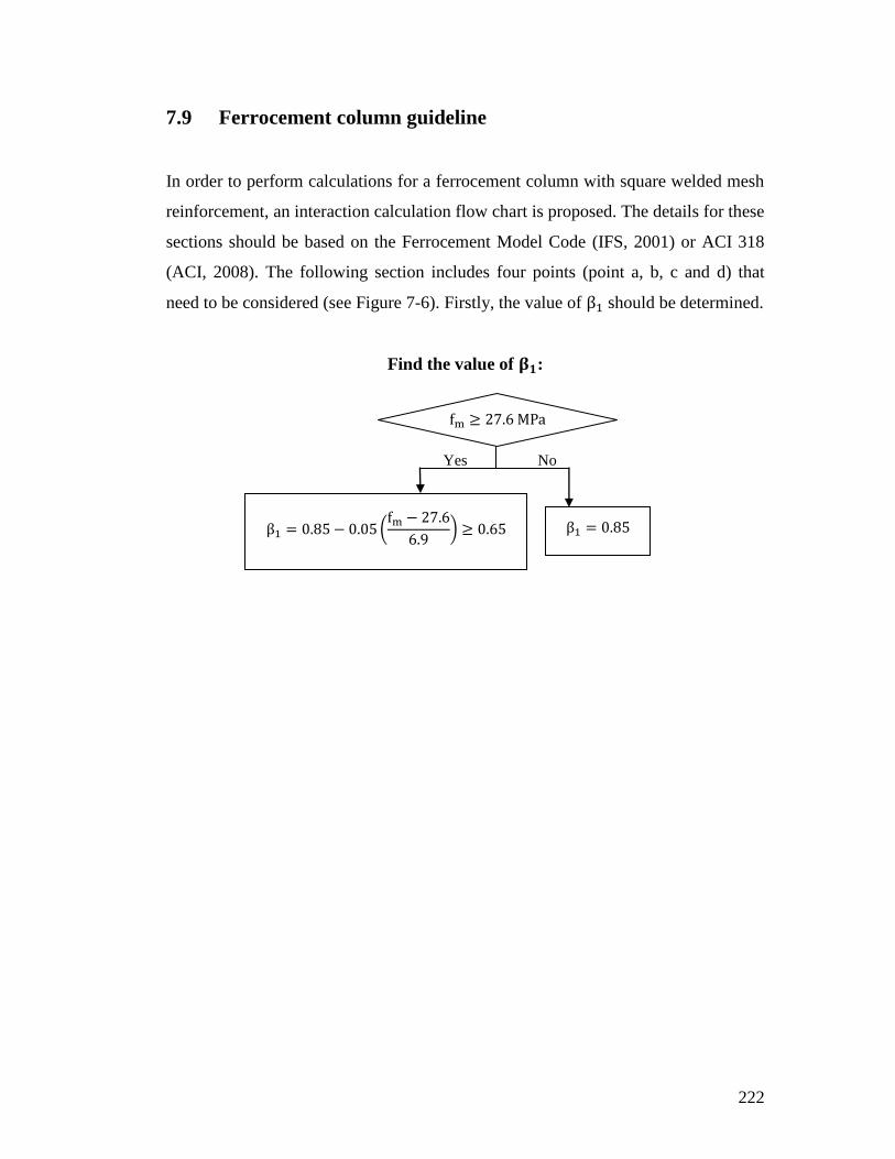
222

7.9 Ferrocement column guideline

In order to perform calculations for a ferrocement column with square welded mesh

reinforcement, an interaction calculation flow chart is proposed. The details for these

sections should be based on the Ferrocement Model Code (IFS, 2001) or ACI 318

(ACI, 2008). The following section includes four points (point a, b, c and d) that

need to be considered (see Figure 7-6). Firstly, the value of should be determined.

Find the value of :

Yes No

223

Point a: Moment strength at zero axial force

Finding Point a

)

)

)

)

Compression ( ) Tension ( )

)

Yes No

224

Point b: Axial compression and moment strength at balanced condition

Finding Point b

)

)

Compression ( ) Tension ( )

)

Yes No

)

)

Yes No

225

Point bc: Axial compression and moment at zero strain

)

Yes No

)

)

Finding Point d

)

226

Point c: Axial compression at zero moment

7.10 Summary

In this chapter, design guidelines for ferrocement columns and reinforced concrete

columns strengthened using ferrocement jackets have been presented. The following

points are emphasized:

Idealization properties of the reinforcing mesh and matrix are used for

design guideline.

For the theoretical interaction diagram for column design, there are three

important points: pure moment, balanced position and pure axial load

An example (FC4) detailed calculation is shown in this chapter.

Comparing the theoretical results with ABAQUS simulation results

shows that the ABAQUS results are higher, because the mesh in the

ferrocement provides confinement. This confinement is not considered

in the theoretical calculations, which therefore underestimate the actual

values.

Non-dimensional interaction diagram for ferrocement columns and

reinforced concrete columns using ferrocement jacket are presented.

Calculation flow chart for the column under pure moment, balanced

point and pure axial load are presented in this chapter.

Finding Point c

End

227

CHAPTER 8 Conclusions and recommendations for

future studies

This chapter presents a summary of the main conclusions from this study and

recommends a number of further studies. Conclusions are drawn from the results

and observations of the experimental work and the finite element analysis (FEA)

presented in this thesis, considering the effect of different parameters of the

ferrocement material.

The present investigation included a set of experimental tests using the following

specimens: reinforced concrete column (RC), ferrocement column (FC) and

reinforced concrete strengthened columns using ferrocement jacket (RFC).

Design guidelines are presented for FC and RFC columns, which are based on the

results of full-scale tests and extensive numerical analyses using FEA. Interaction

diagrams for ferrocement columns and reinforced concrete columns strengthened

using ferrocement jackets are developed, based on the design of conventional

reinforced concrete columns in Eurocode 2 (CEN, 2004a) and ACI 318 (ACI, 2008).

8.1 Summary

8.1.1 Experimental results

Material property tests have been conducted, including concrete, matrix, 12 mm

diameter steel bar (longitudinal ribbed bar in RC), 3 mm diameter bar (transverse bar

in RC) and welded mesh. The concrete and matrix property tests included

compression and split tests using 100 200 mm cylinders.

228

Eight columns were cast: 2 reinforced concrete columns, 4 ferrocement columns and

2 strengthened reinforced concrete columns using ferrocement jackets. For safety

and operability, all specimens were tested in a horizontal cantilever position; two

Macalloy bars applied a constant axial load (200 kN) and an actuator applied lateral

load.

The lateral load was either static or cyclic. For the static load tests, the actuator was

moved at 0.5 mm/s. For the cyclic load tests, a load was applied at a frequency of

1 Hz with an amplitude (A) which was set at the displacement value corresponding

to 60% of the ultimate load from the static test. Linpots were used to measure the

downward movement of the specimens. They were arranged in two parallel lines

initially to check for any twist that may have been occurring. A final arrangement of

just one row along the length of the column was adopted, as no significant twist was

observed. Also, a movement of the top fixed-end plate was observed during the

initial test, hence two extra linpots were added in order to calculate an effective

support stiffness. This support stiffness was incorporated in the FEA using two

springs.

Static column tests:

Firstly, the result of the initial linpots arrangement showed that there was no twisting

of the specimen. The support condition was semi-rigid with an effective rotational

stiffness of 2075 kNm/rad (the detail calculation is shown in Appendix I). Two

linear springs were used in the numerical model to simulate the support flexibility

(see § 4.3)

Specimen FC2 had the lowest lateral load capacity of 29 kN, whereas Specimen

RFC3 had the highest value of 58 kN. The capacity of Specimen FC4 was 20%

higher than FC2. RFC2 and RFC3 had significantly increased peak lateral loads than

RC, which shows that the ferrocement jacket has a significant potential for

strengthening reinforced concrete columns (35.7 kN for RC).

229

As the end support was not totally restrained, the resulting displacement was split

into two parts reflecting: the support rotation effect and the bending-shear effect. For

all columns, the support rotation effect dominated until the lateral load reached

approximately 90% of the peak load. However, the values of initial stiffness were

similar.

The deformation ductility was calculated using the energy balanced method. FC4

and RFC3 have higher values of ductility than FC2 and RFC2, respectively. Higher

amounts of mesh results have greater deformation ductility.

Cyclic column tests:

The displacement amplitudes for RC, FC2-C and FC4-C were 14.5 mm, 12.5 mm

and 14.0 mm. Results were recorded after 100, 200, 400 and 600 cycles, during

cyclic loading. The columns exhibited reduced lateral load capacity with increasing

number of cycles. After 600 cycles of loading, the peak load reduced significantly

for RC-C and FC2-C, by 21% and 24% respectively. But for FC4-C it just reduced

by 11% of the peak lateral load. Then a further 400 cycles were applied, and the

capacity reduced to 67%. With higher amounts of mesh, the specimens showed

lower load reduction in percentages.

The stiffnesses during cyclic test also reduced with increasing number of cycles. The

stiffness for RC-C dropped much quicker than those for the ferrocement specimens.

After 600 cycles, the stiffness of RC-C and FC2 showed a similar degradation to

71%, and 79%for FC4-C. Higher amounts of mesh provided higher resistance for

both peak lateral load and initial stiffness.

8.1.2 Finite element modelling analysis and parametric studies

The results from the experimental work were used to validate the FEA models. A

concrete damaged plasticity (CDP) model was used in this thesis. Concrete and

matrix were modelled using C3D8R elements, and the reinforcements were

230

modelled using truss element T3D2. The compressive behaviour of concrete and the

matrix were characterized by Eurocode 2 (CEN, 2004a) and Popovics (1973)

model, respectively. The tensile behaviour used the Wang and Hsu (2001)

model. The reinforcing mesh was embedded in the concrete or matrix section, and

for RFC2 and RFC3, the constraint between the concrete surface and the matrix

surface was chosen to be a “Tie”.

Five plasticity parameters for CDP were analysed and validated, including dilation

angle, eccentricity, σ σ , Kc and viscosity parameter, also the finite element

mesh size and value of spring stiffness were analysed. After conducting a mesh

sensitivity analysis, the size of the finite element mesh for concrete and matrix was

selected as 30 mm and the reinforcing mesh was selected to be 12.6 mm. The

support flexibility was introduced by two springs, the stiffnesses of which were

calculated from the measured displacement values.

The calculated load-deflection curves for RC, FC and RFC showed a high degree of

correlation with the measured curves (less than 10% differences). The contour plots

of strain for each column indicated the position of cracks. For RFC2 and RFC3, the

initial stiffness from FEA are higher than experimental tests, possibly because: i) the

embedded interaction used in the FEA is too perfect to simulate the realistic cases as

bond-slip may occur, ii) material properties cannot be perfectly input in ABAQUS,

iii) spring setting in ABAQUS may not totally describe the experimental tests.

Extensive parametric studies were undertaken to investigate the effects of different

variables, including column end-conditions, value of axial load, length of column,

the material properties (concrete, matrix, main bar, stirrups and welded mesh) and

reinforcement detail (amount, arrangement and position) . The support condition was

considered as encastre as the rotationally flexible support in the current set up is an

artefact of the short column size and the type of reaction frame that was chosen.

Four different grades of concrete or matrix were analysed, C30, C38, C40 and C50

for concrete; and M40, M50, M60 and M62 for matrix. The experimental values

231

were C38 and M62. Increases in the grade of concrete or matrix, increased the peak

lateral load. Also, for the main bar and welded mesh, increasing the material grade

also increased the peak lateral load. With increases of the cross-section of the main

bar or welded mesh, the lateral load was raised. However, the grade and cross-

section of stirrups had negligible affect on the value of the peak load.

Varying the axial load produced significant changes in the value of the peak lateral

load. The values of lateral loads and axial loads make up the interaction diagram.

The interaction diagrams for ferrocement (FC2 and FC4) are similar; with FC4

having 10% greater lateral load than FC2 at the balanced point. Higher amounts of

mesh had greater moments.

8.1.3 Design guide

The idealised properties of the reinforcing mesh and matrix were used for design

guidelines. Popovics (1973) model was used for properties of the matrix. For the

theoretical interaction diagram for column design, there are three important points:

pure moment, balanced position and pure axial load. The position of neutral axis

(N.A) needs to be calculated first followed by the calculation of forces for each

mesh strand and compressive forces in concrete or matrix. An example of detailed

calculation for FC4 is shown in Chapter 7.

The ABAQUS simulations show higher capacity than the theoretical results, because

the mesh in the ferrocement provides confinement. This confinement was not

considered in the theoretical calculations, which therefore underestimate the actual

values to the safe side for design purposes. Dimensionless interaction diagrams for

FC and RFC column are presented.

232

8.2 Conclusion

The main conclusions from this thesis are: Ferrocement may be successfully used to

add strength and ductility to columns either when used in place of normal

longitudinal reinforcement or when used as a retrofit coating.

1. Higher amounts of mesh result in greater deformation ductility.

2. Higher amounts of mesh provide higher peak lateral loads and initial

stiffness.

3. In all cases after cyclic loading the peak-load and stiffness reduced.

4. ABAQUS simulation can successfully predict deflection results.

5. The theoretical values based on ACI are conservative.

6. Non-dimensional interaction diagram for ferrocement columns and

reinforced concrete columns using ferrocement jacket are presented.

7. Calculation flow chart for the column under pure moment, balanced point

and pure axial load are presented.

8.3 Recommendations for future study

This study highlighted the behaviour of square columns under axial load and

moment. Due to financial and time constraints, only five static tests were performed,

and more experimental tests are needed changing the shape and dimensions, such as

circular or longer columns. Different kinds of mesh (such as woven mesh) of

ferrocement also need to be considered. The cyclic load application for RFC column

may need to be considered.

233

The numerical simulation was carried out using ABAQUS, which was available to

the author, but alternative numerical simulation software, such as DIANA, may be

more suitable because it can show cracking by physical separation of the elements.

The cyclic loading tests of ferrocement column also need to be studied by FEA.

The design guideline is limited to a box-section of welded mesh column, and needs

to be expanded for ferrocement beams or other sections. Strengthened beams or

floors, using ferrocement jackets or ferrocement layers, may need to be tested and

modelled and developed into design guidelines.

234

References

ABAQUS 2009. Version 6.8, ABAQUS Documentation. USA: ABAQUS Inc.

American Concrete Institute (ACI), 2008. Building Code Requirements for

Structural Concrete (ACI 318-08) and Commentary (ACI 318R-05). Detroit,

American Concrete Institute.

American Concrete Institute (ACI), 1997a. Guide for Repair of Concrete Bridge

Superstructures. ACI 546.1R-80, Detroit, American Concrete Institute.

American Concrete Institute (ACI), 1988. Guide for the Design, Construction, and

Repair of Ferrocement. ACI 549, Detroit, American Concrete Institute.

American Concrete Institute (ACI), 1997b. State-of-The-art Report on Ferrocement.

ACI 549R-97, Detroit, American Concrete Institute.

AHMED, T., ALI, S. & CHOUDHURY, J. Experimental study of ferrocement as a

retrofit material for masonry columns, Ferrocement International Symposum, 1994.

269-276.

AL-KUBAISY, M. & NEDWELL, P., 1999. Behavior and strength of ferrocement

rectangular beams in shear. Journal of Ferrocement, 29 (1), 1-16.

ARIF, M. & KAUSHIK, S. K., 1999. Mechanical behaviour of ferrocement

composites: an experimental investigation. Cement and Concrete Composites, 21 (4),

301-312.

BALAGURU, P. N., SHAH, S. P. & NAAMAN, A. E., 1979. Fatigue behavior and

design of ferrocement beams. Journal of the Structural Division, 105 (7), 1333-1346.

BARRERA, A., BONET, J., ROMERO, M. & MIGUEL, P., 2011. Experimental

tests of slender reinforced concrete columns under combined axial load and lateral

force. Engineering Structures, 33 (12), 3676-3689.

BARRERA, A. C., BONET, J. L., ROMERO, M. L. & FERN NDEZ, M. A., 2012.

Ductility of slender reinforced concrete columns under monotonic flexure and

constant axial load. Engineering Structures, 40 (0), 398-412.

British Stand Institution (BSI), 2006. Method of specifying and guidance for the

specifier. BS 8500, Londom, British Stand Institution.

British Stand Institution (BSI), 2009. Testing fresh concrete. Sampling. BS EN

12350, Lodnon, British Stand Institution.

British Stand Institution (BSI), 2010. Testing hardened concrete. Shape, dimensions

and other requirements for specimens and moulds. BS EN 12390, London, British

Stand Institution.

235

BSS, http://www.bsspatterdalehall.com/tenacity-of-bolton/gallery/year-8-2009

[Online]. Bolton School Services (BSS).

CAMBODIA, http://www.ewb.org.au/opportunities/50/10205 [Online].

CAPRANI, C., 2006. Civil Engineering Design (1) Design of Reinforced Concrete

Columns.

CEN, 2004a. Eurocode 2: Design of Concrete Structures: Part 1-1: General Rules

and Rules for Buildings.

CEN, 2004b. Eurocode 8: Design of structures for earthquake resistance—Part 1:

General rules, seismic actions and rules for buildings.

DESAYI, P. & JOSHI, A. D., 1976. Ferrocement load-bearing wall elements.

Journal of the Structural Division, 102 (9), 1903-1916.

DETWILER, R. J. & MEHTA, P. K., 1989. Chemical and physical effects of silica

fume on the mechanical behavior of concrete. ACI Materials Journal, 86 (6).

DODSON, V. H. 1990. Concrete admixtures, Van Nostrand Reinhold New York.

DRUCKER, D. C. & PRAGER, W., 2013. Soil mechanics and plastic analysis or

limit design. Quarterly of applied mathematics, 10.

EXPANDED-MESH,

http://www.makewiremesh.com/Expanded%20Metal%20Mesh.htm [Online].

FAHMY, E. H., ABOU ZEID, M. N., SHAHEEN, Y. B. & GAAFAR, H., 2005.

Behavior of ferrocement panels under axial and flexural loadings. The 33rd annual

general conference of the canadian society for civil engineering.

FERROCEMENT.COM, http://ferrocement.com/bioFiber/roofLabContents-

y5.en.html [Online].

FERROCEMENT SOCIETY (FS), 2013. 2ND NATIONAL CONVENTION. Pune,

India.

GIONCU, V. & MAZZOLANI, F. 2003. Ductility of seismic-resistant steel

structures, Taylor & Francis.

HEXAGONAL-MESH, http://fencingwire.net/chichen-mesh [Online].

HOOTON, R., 1993. Influence of silica fume replacement of cement on physical

properties and resistance to sulfate attack, freezing and thawing, and alkali-silica

reactivity. ACI Materials Journal, 90 (2).

http://www.bsspatterdalehall.com/tenacity-of-bolton/gallery/year-8-2009

http://www.ewb.org.au/opportunities/50/10205

http://www.makewiremesh.com/Expanded%20Metal%20Mesh.htm

http://ferrocement.com/bioFiber/roofLabContents-y5.en.html

http://ferrocement.com/bioFiber/roofLabContents-y5.en.html

http://fencingwire.net/chichen-mesh

236

HUQ, S. & PAMA, R. P., 1978. Ferrocement in tension: analysis and design.

Journal of Ferrocement, 8 (3), 143-168.

International Ferrocement Society (IFS), 2001. Ferrocement Model Code. Naaman,

AE. Balaguru, P. Nassif, H. Pama, R. Tatsa, E. Austriaco, LR. Hanai, JB. Nedwell, P.

Paramasivam, P.

JADFERROCEMENTS.NET, http://www.jadferrocements.net/repairs-

rehabilitation-retrofitting.html [Online].

JOHNSTON, C. D. & MATTAR, S. G., 1976. Ferrocement—Behavior in Tension

and Compression. Journal of the Structural Division, 102 (5), 875-889.

KAISH, A. B. M. A., ALAM, M. R., JAMIL, M. & WAHED, M. A., 2013.

Ferrocement Jacketing for Restrengthening of Square Reinforced Concrete Column

under Concentric Compressive Load. Procedia Engineering, 54 (0), 720-728.

KHANZADI, M. & RAMESHT, M., 1996. The effect of cover and arrangement of

reinforcement on the behavior of ferrocement in tension. Journal of Ferrocement, 26

(2), 85-94.

KIM, J.-K. & LEE, S.-S., 2000. The behavior of reinforced concrete columns

subjected to axial force and biaxial bending. Engineering Structures, 22 (11), 1518-

1528.

MANSUR, M. & ONG, K., 1987. Shear strength of ferrocement beams. ACI

Structural Journal, 84 (1).

MANSUR, M. & PARAMASIVAM, P., 1985. Ferrocement under combined

bending and axial loads. International Journal of Cement Composites and

Lightweight Concrete, 7 (3), 151-158.

MORAGE, S. Element De Ferrocemento Para Vivienda social.In: RIVAS, H. W.,

ed., 10th International Symposium on Ferrocement and Thin Reinforced Cement

Composites (FERRO 10), 2012 La Havana, Cuba.

MOURAD, S. & SHANNAG, M., 2012. Repair and strengthening of reinforced

concrete square columns using ferrocement jackets. Cement and Concrete

Composites, 34 (2), 288-294.

NAAMAN, A. E. 2000. Ferrocement and laminated cementitious composites,

Techno press.

NAAMAN, A. E. & SHAH, S. P. Tensile tests of ferrocement, ACI Journal

Proceedings, 1971. American Concrete Institute.

http://www.jadferrocements.net/repairs-rehabilitation-retrofitting.html

http://www.jadferrocements.net/repairs-rehabilitation-retrofitting.html

237

NASSIF, H. H. & NAJM, H., 2004. Experimental and analytical investigation of

ferrocement–concrete composite beams. Cement and Concrete Composites, 26 (7),

787-796.

NATHAN, G. & PARAMASIVAM, P., 1974. Mechanical properties of ferrocement

materials. Proc. 1st Australian Conj. on Engineering Materials, 309-31.

NEDWELL, P., 2009. Ferrocement Lecture Lecture PowerPoint. University of

Manchester, 64.

NEDWELL, P., RAMESHT, M. & RAFEI-TAGHANAKI, S. Investigation into the

repair of short square columns using ferrocement, FERROCEMENT

INTERNATIONAL SYMPOSIUM, 1994. 277-285.

NERVI, P. L., SALVADORI, M. & SALVADORI, G. 1956. Structures, FW Dodge

Corporation New York.

PAILL RE, A.-M. 1995. Application of Admixtures in Concrete: State-of-the Art

Report, Taylor & Francis.

PARK, R., PRIESTLEY, M. & GILL, W. D., 1982. Ductility of square-confined

concrete columns. Journal of the Structural Division, 108 (4), 929-950.

PAUL, B. K. & PAMA, R. P. 1978. Ferrocement, International Ferrocement

Information Center, Asian Institute of Technology Bangkok, Thailand.

POPOVICS, S., 1973. A numerical approach to the complete stress-strain curve of

concrete. Cement and concrete research, 3 (5), 583-599.

RIVAS, H. W. & HERNANDEZ, Y.-L. L. Sistema De Edificios Residenciales

Sismoresistentes De Ferrocemento: Una Opcion Paea La Construccion De Viviendas

De Interes Social In: RIVAS, H. W., ed., 10th International Symposium on

Ferrocement and Thin Reinforced Cement Composites, 2013 La Havana, Cuba.

SHANNAG, M. & MOURAD, S., 2012. Flowable high strength cementitious

matrices for ferrocement applications. Construction and Building Materials, 36,

933-939.

TAKIGUCHI, K., 2003. An investigation into the behavior and strength of

reinforced concrete columns strengthened with ferrocement jackets. Cement and

Concrete Composites, 25 (2), 233-242.

TIAN, S., 2013. Shear Behaviour of Ferrocement Deep Beams. University of

Manchester.

WALKUS, B. & KOWALSKI, T., 1971. Ferrocement: A survey. Concrete Cement-

Concrete Association of London, 48-52.

238

WANG, T. & HSU, T. T., 2001. Nonlinear finite element analysis of concrete

structures using new constitutive models. Computers & structures, 79 (32), 2781-

2791.

WELDED-MESH, http://www.haoyuwire.com/Stainless-steel-welded-mesh.htm

[Online].

WOVEN-MESH, http://www.galvanized-wiremesh.com/square-wire-mesh.htm

[Online].

YAQUB, M., BAILEY, C., NEDWELL, P., KHAN, Q. & JAVED, I., 2013.

Strength and stiffness of post-heated columns repaired with ferrocement and fibre

reinforced polymer jackets. Composites Part B: Engineering, 44 (1), 200-211.

http://www.haoyuwire.com/Stainless-steel-welded-mesh.htm

http://www.galvanized-wiremesh.com/square-wire-mesh.htm

239

Appendix A. Reinforcement properties

Figure A-1: Stress-strain curves for 12 mm diameter Steel bar

Figure A-2: Stress-strain curves for 3 mm diameter stirrup

0

100

200

300

400

500

600

700

800

0 0.02 0.04 0.06 0.08 0.1 0.12 0.14 0.16

Str

ess

(MP

a)

Strain

12 mm Steel bar-01

12 mm Steel bar-02

12 mm Steel bar-03

0

100

200

300

400

500

600

700

800

0 0.01 0.02 0.03 0.04 0.05 0.06 0.07 0.08

Str

ess

(MP

a)

Strain

3 mm Stirrup-01

3 mm Stirrup-02

3 mm Stirrup-03

240

Figure A-3: Stress-strain curves for 1.6 mm diameter welded mesh

0

100

200

300

400

500

0 0.05 0.1 0.15 0.2

Str

ess

(MP

a)

Strain

1.6 mm welded mesh-01

1.6 mm welded mesh-02

241

Appendix B. The dimensions of the specimens

Figure B-4: View of the specimen, showing the top, bottom, front and back

RC view Width (mm) Length

(mm)

Weight

(kg) Left Middle Right Average

Top 150 151 152 151.0 1020

62.3 Bottom 150 151 151 150.7 1021

Front 150 150 151 150.3 1020

Back 150 150 151 150.3 1020

RC-C view Width (mm) Length

(mm)

Weight


Top 151 151 152 151.3 1020

61.9 Bottom 151 151 152 151.3 1021

Front 151 151 152 151.3 1021

Back 151 151 151 151.0 1020

FC2 view Width (mm) Length

(mm)

Weight


Top 150 151 151 150.7 1020

57.3 Bottom 150 151 151 150.7 1021

Front 151 151 151 151.0 1021

Back 150 150 151 150.3 1020

Fixed-end area

Axial load (P)

Loading area

Lateral load (V)

Front (red rectangular)

Back Top

Bottom

242

FC2-C view Width (mm) Length

(mm)

Weight


Top 151 151 151 151.0 1020

58.4 Bottom 151 151 151 151.0 1021

Front 151 151 151 151.0 1021

Back 150 151 151 150.7 1021

FC4 view Width (mm) Length

(mm)

Weight


Top 151 151 151 151.0 1020

60.6 Bottom 151 151 151 151.0 1020

Front 151 151 151 151.0 1021

Back 151 151 151 151.0 1021

FC4-C view Width (mm) Length

(mm)

Weight


Top 151 152 152 151.3 1021

61.6 Bottom 151 151 152 151.3 1021

Front 151 151 152 151.3 1021

Back 151 151 152 151 1021

RFC2 view

Width (mm) Length

(mm)

Weight

(kg) Left Left

middle Middle

Right

Middle Right Average

Top 181 180 182 181 181 181 1019

96.3 Bottom 178 179 180 180 179 179.2 1020

Front 179 179 180 181 180 179.8 102

Back 180 182 181 180 181 180.8 1019

RFC3 view

Width (mm) Length

(mm)

Weight

(kg) Left Left

middle Middle

Right

Middle Right Average

Top 181 180 182 181 181 181 1019

97.6 Bottom 178 179 180 180 179 179.2 1020 Front 179 179 180 181 180 179.8 102 Back 180 182 181 180 181 180.8 1019

243

Appendix C. The specimens after the tests

Figure C-5: The two-layer mesh ferrocement failure after testing (FC2)

244

Figure C-6: The four-layer mesh ferrocement failure after testing (FC4)

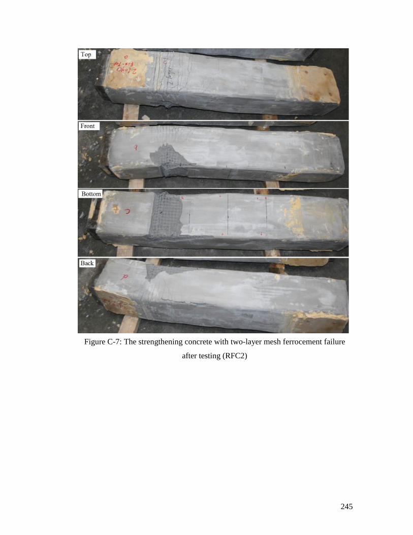
245

Figure C-7: The strengthening concrete with two-layer mesh ferrocement failure

after testing (RFC2)

246

Figure C-8: The strengthening concrete with three-layer mesh ferrocement failure

after testing (RFC3)

247

Appendix D. Support rotation and bending-shear effect

Support rotation effect simplified diagram:

Figure D-9: Simplified support rotation effect diagram

Reinforced concrete (RC):

At 0.33peak load of RC is 0.33 35.7=11.9 kN

Figure D-10: The cross section of RC

150 mm

20 mm

O

nA

720 mm

92.5 mm

1020 mm

200 mm

F1 F2 V

100 mm

150 m

m

248

Then:

3.47 mm

Bending-shear effect: The bending deflection of the specimen acting as a

concentrated load working on a cantilever beam, can be calculated as:

)

Where:

Length of the cantilever, 812.5 mm

h Width of column, 150 mm

Lateral load, 0.33 of peak load, 12 kN

Young's Modulus of composite

Second moment area

Young's Modulus of concrete

Young's Modulus of steel bar

Elastic moduli ratio to matrix:

)

)

)

Then:

)

249

Ferrocement with two-layers mesh (FC2) and four-layers mesh (FC4)

At 0.33peak load of FC2 is 0.33 29.0=9.7 kN

At 0.33peak load of FC4 is 0.33 35=11.6 kN

Assumed the mesh layer is distributed uniformly. The skeleton of welded mesh is

simplified as one-layer. The distances of the mesh from the extreme tensile surface

are called ( , , ,......, , ), in which has 3.5 mm (cover),

has 3.5+12.6 1=16.1 mm, has 3.5+12.6 2=28.7 mm, etc., the last one is .

Figure D-11: The cross section for FC

Then: Then:

2.82 mm 3.38 mm

150 mm

150 m

m

ds1

ds2

ds3

ds4

ds12

250

Young's Modulus of matrix

Young's Modulus of mesh

Elastic moduli

ratio to matrix Mesh: =

Cross-section area (mm2)

Mesh level

As1 and As12 48.3 96.5

As2, As3, As4,......As11, As11 8.04 16.1

)

) )

)

)

)

) )

)

)

Then:

)

)

251

Reinforced concrete strengthened using a ferrocement jacket: with two-layers

mesh (RFC2) and three-layers mesh (RFC3)

0.33 peak load of RFC2 (0.33 50.9=17.0 kN)

0.33 peak load of RFC3 (0.33 57.7=19.2 kN)

Also, assumed the mesh layer is distributed uniformly. The skeleton of welded mesh

is simplified as one-layer. Similarly to FC2 or FC4, the distances of the mesh from

the extreme tensile surface are called ( , , ,......, , )

Figure D-12: The cross section for RFC

Then: Then:

4.90 mm 5.53 mm

ds1

150 m

m

150 m

m

180 m

m

15 mm

150 mm

20 mm

ds2

1 ds3

21 ds4

21

ds14

ds15

180 mm

252

Young's Modulus of matrix

Young's Modulus of concrete

Young's Modulus of steel bar

Young's Modulus of mesh

Elastic moduli

ratio to matrix

Concrete: =

Mesh: =

Steel bar: =

Cross-section area (mm2)

Mesh level As1 and As15 96.5 96.5

As2, As3, As4,......As13, As14 12.1 16.1

)

) )

)

)

)

) )

)

)

253

Then:

)

)

Comparing the bending-shear effect with , shows the results to be quite different.

So the author decided to re-calculate with the tensile force of the matrix and concrete

ignored.

)

) )

)

)

)

) )

)

)

Then:

)

)

254

Appendix E. Test results for all the linpots

Figure E-13: Load-displacement curves at different positions (FC2)

Figure E-14: Load-displacement curves at different positions (FC4)

0

5

10

15

20

25

30

35

40

0 10 20 30 40

La

tera

l lo

ad

(k

N)

Displacement (mm)

FC2: Li1

FC2: Li2

FC2: Li3

FC2: Li4

FC2: Li5

FC2: Li6

FC2: Li7

FC2: Li-A

0

5

10

15

20

25

30

35

40

0 10 20 30 40

La

tera

l lo

ad

(k

N)

Displacement (mm)

FC4: Li1

FC4: Li2

FC4: Li3

FC4: Li4

FC4: Li5

FC4: Li6

FC4: Li7

FC4: Li-A

255

Figure E-15: Load-displacement curves at different positions (RFC2)

Figure E-16: Load-displacement curves at different positions (RFC3)

0

10

20

30

40

50

60

70

0 10 20 30 40 50 60 70 80

La

tera

l lo

ad

(k

N)

Displacement (mm)

RFC2: LiF1/LiB1 RFC2: LiF2/LiB2 RFC2: LiF3/LiB3 RFC2: LiF4/LiB4 RFC2: Li-A

0

10

20

30

40

50

60

70

0 10 20 30 40 50 60 70 80

La

tera

l lo

ad

(k

N)

Displacement (mm)

RFC3: Li1

RFC3: Li2

RFC3: Li3

RFC3: Li4

RFC3: Li5

RFC3: Li6

RFC3: Li7

RFC3: Li-A

256


bending-shear effect at Li-A (FC2 and FC4)


bending-shear effect at Li-A (RFC2 and RFC3)

0

5

10

15

20

25

30

35

40

0 10 20 30 40 50

La

tera

l lo

ad

(k

N)

Displacement (mm)

Total displacement (FC2)

Support rotation effect (FC2)

Bending and shear effect (FC2)

Total displacement (FC4)

Support rotation effect (FC4)

Bending and shear effect (FC4)

0

10

20

30

40

50

60

70

0 10 20 30 40 50 60 70 80

La

tera

l lo

ad

(k

N)

Displacement (mm)

Total displacement (RFC2)

Support rotation effect (RFC2)

Bending and shear effect (RFC2)

Total displacement (RFC3)

Support rotation effect (RFC3)

Bending and shear effect (RFC3)

257

Figure E-19: Displacement for each linpot at different loads (FC2)

Figure E-20: Displacement for each linpot at different loads (FC4)

-5

0

5

10

15

20

25

30

35

40

45

0 200 400 600 800 1000

Dis

pla

cem

ent

(mm

)

Position (mm)





0.33 peak load

0.66 peak load

Peak load

Failure

-5

0

5

10

15

20

25

30

35

40

45

0 200 400 600 800 1000

Dis

pla

cem

ent

(mm

)

Position (mm)





0.33 peak load

0.66 peak load

Peak load

Failure

258

Figure E-21: Displacement for each linpot at different loads (RFC2)

Figure E-22: Displacement for each linpot at different loads (RFC3)

-10

0

10

20

30

40

50

60

70

80

0 200 400 600 800 1000

Dis

pla

cem

ent

(mm

)

Position (mm)





0.33 peak load

0.66 peak load

Peak load

Failure

-10

0

10

20

30

40

50

60

70

80

0 200 400 600 800 1000

Dis

pla

cem

ent

(mm

)

Position (mm)





0.33 peak load

0.66 peak load

Peak load

Failure

259

Lateral load and stiffness of RC-C, FC2-C, FC4-C during number of cycles

Figure E-23: Lateral load during tests with number of cycles

Table E-1: Result of lateral load and degradation of RC-C, FC2-C and FC4-C during

cyclic loading

No.

of

cycles

RC-C FC2-C FC4-C

V (kN) Degradation

(%) V (kN)

Degradation

(%) V (kN)

Degradation

(%)

First 26.6 100% 22.2 100% 25.0 100%

100 24.8 93% 20.0 90% 23.2 93%

200 23.5 88% 19.2 87% 22.7 91%

400 22.5 84% 17.1 77% 22.4 90%

600 20.9 79% 16.8 76% 22.2 89%

1000

16.8 67%

Note: the mark ‘V’ is lateral load

0

5

10

15

20

25

30

0 100 200 300 400 500 600 700 800 900 1000

La

tera

l lo

ad

(k

N)

Number of cycles

Load (RC-C)

Load (FC2-C)

Load (FC4-C)

260

Figure E-24: Stiffness during tests with number of cycles

Table E-2: Result of stiffness and degradation of RC-C, FC2-C and FC4- C during

cyclic loading

No.

of

cycles

RC-C FC2-C FC4-C

Stiffness

(kN/mm)

Degradation

(%)

Stiffness

(kN/mm)

Degradation

(%)

Stiffness

(kN/mm)

Degradation

(%)

First 2.50 100% 2.60 100% 2.53 100%

100 2.00 80% 2.39 92% 2.30 91%

200 1.95 78% 2.31 89% 2.24 89%

400 1.84 74% 1.99 77% 2.07 82%

600 1.77 71% 1.87 72% 1.99 79%

1000

1.52 60%

0.0

0.5

1.0

1.5

2.0

2.5

3.0

0 100 200 300 400 500 600 700 800 900 1000

Sti

ffn

ess

(kN

/mm

)

Number of cycles

Stiffness (RC-C)

Stiffness (FC2-C)

Stiffness (FC4-C)

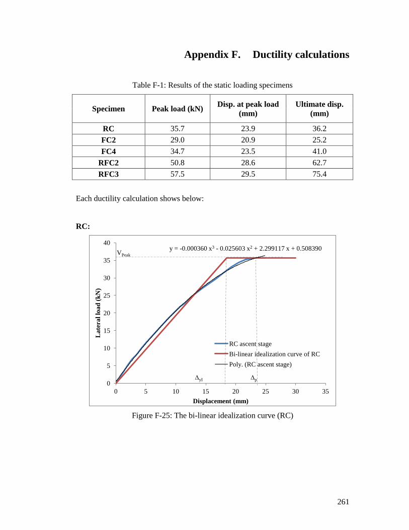
261

Appendix F. Ductility calculations

Table F-1: Results of the static loading specimens

Specimen Peak load (kN) Disp. at peak load

(mm)

Ultimate disp.

(mm)

RC 35.7 23.9 36.2

FC2 29.0 20.9 25.2

FC4 34.7 23.5 41.0

RFC2 50.8 28.6 62.7

RFC3 57.5 29.5 75.4

Each ductility calculation shows below:

RC:

Figure F-25: The bi-linear idealization curve (RC)

y = -0.000360 x3 - 0.025603 x2 + 2.299117 x + 0.508390

0

5

10

15

20

25

30

35

40

0 5 10 15 20 25 30 35

La

tera

l lo

ad

(k

N)

Displacement (mm)

RC ascent stage

Bi-linear idealization curve of RC

Poly. (RC ascent stage)

VPeak

∆yI ∆p

262

So the area of above x-axis equal to the trapezoid:

)

)

Put the values in the equation, then: =18.6 mm.

The ductility value will be:

μ

FC4: (the FC2 is shown in § 4.8)

Figure F-26: The bi-linear idealization curve (FC4)

y = 0.000289 x3 - 0.057643 x2 + 2.659578 x - 0.125228

0

5

10

15

20

25

30

35

40

0 5 10 15 20 25 30 35

La

tera

l lo

ad

(k

N)

Displacement (mm)

FC4 ascent stage


Poly. (FC4 ascent stage)

∆yI ∆p

VPeak

263

So the area of above the x-axis is equal to the trapezoid:

)

)



μ

RFC2:

Figure F-27: The bi-linear idealization curve (RFC2)

y = -0.000603 x3 + 0.005532 x2 + 2.034539 x - 1.208304

0

10

20

30

40

50

60

0 5 10 15 20 25 30 35 40 45

La

tera

l lo

ad

(k

N)

Displacement (mm)

RFC2 ascent stage

Bi-linear idealization curve of RFC2

Poly. (RFC2 ascent stage)

∆yI ∆p

VPeak

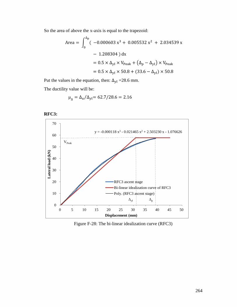
264


)

)



μ

RFC3:

Figure F-28: The bi-linear idealization curve (RFC3)

y = -0.000118 x3 - 0.021465 x2 + 2.503230 x - 1.076626

0

10

20

30

40

50

60

70

0 5 10 15 20 25 30 35 40 45 50

La

tera

l lo

ad

(k

N)

Displacement (mm)

RFC3 ascent stage

Bi-linear idealization curve of RFC3

Poly. (RFC3 ascent stage)

∆yI ∆p

VPeak

265


)

)



μ

266

Appendix G. Full details of the changing parameters

Table G-1: Details of the FEM parameters for RC

RC Axial

load

(kN)

Concrete

property

(MPa)

Steel bar

property

(MPa)

Total

area

of

steel

bars

(mm2)

Number

of steel

bar

Stirrup

property

(MPa)

Cross-

section

area of

stirrup

(mm2)

Axial load

(kN)

0 38 480 452 4 600 7.07

100 38 480 452 4 600 7.07

200 38 480 452 4 600 7.07

300 38 480 452 4 600 7.07

400 38 480 452 4 600 7.07

500 38 480 452 4 600 7.07

600 38 480 452 4 600 7.07

800 38 480 452 4 600 7.07

Concrete

property

200 30 480 452 4 600 7.07

200 40 480 452 4 600 7.07

200 50 480 452 4 600 7.07

Steel bar

property

200 38 275 452 4 600 7.07

200 38 355 452 4 600 7.07

200 38 525 452 4 600 7.07

Total area

of steel

bars (mm2)

200 38 480 679 4 600 7.07

200 38 480 905 4 600 7.07

Number of

steel bar 200 38 480 905 8 600 7.07

Size of

stirrups

200 38 480 452 4 275 7.07

200 38 480 452 4 355 7.07

200 38 480 452 4 525 7.07

Cross-

section

area of

stirrup

(mm)

200 38 480 452 4 600 14.1

200 38 480 452 4 600 28.3

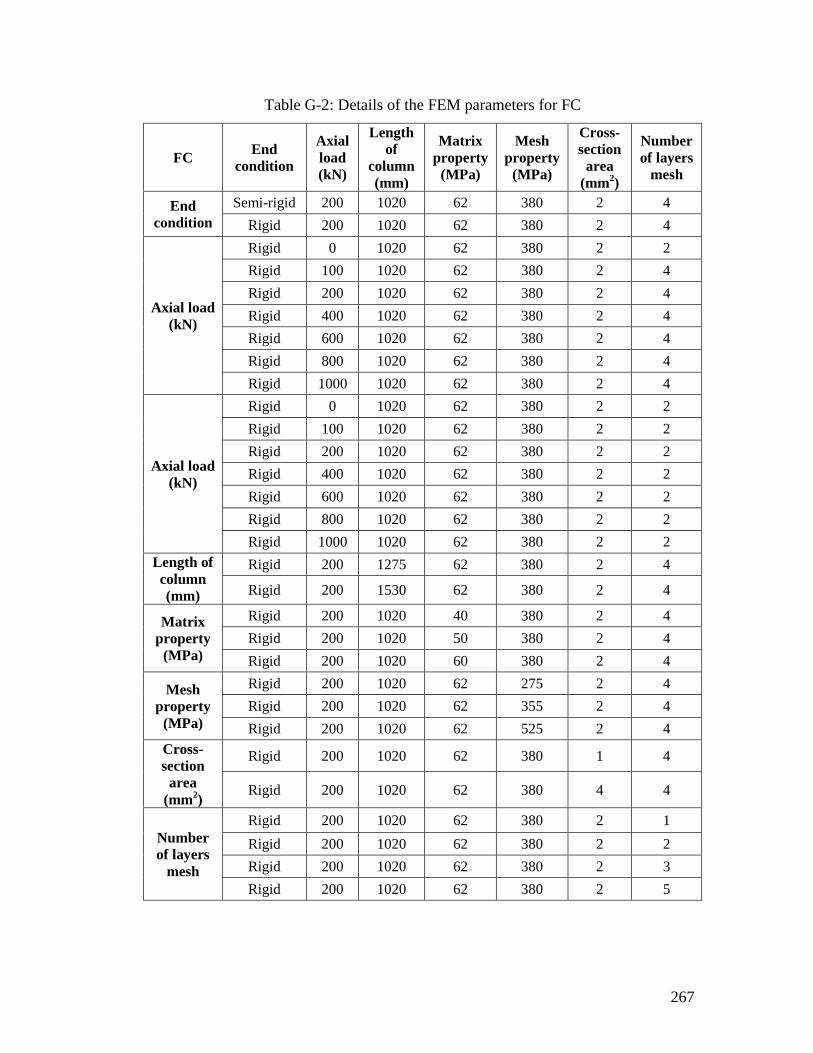
267

Table G-2: Details of the FEM parameters for FC

FC End

condition

Axial

load

(kN)

Length

of

column

(mm)

Matrix

property

(MPa)

Mesh

property

(MPa)

Cross-

section

area

(mm2)

Number

of layers

mesh

End

condition

Semi-rigid 200 1020 62 380 2 4

Rigid 200 1020 62 380 2 4

Axial load

(kN)

Rigid 0 1020 62 380 2 2

Rigid 100 1020 62 380 2 4

Rigid 200 1020 62 380 2 4

Rigid 400 1020 62 380 2 4

Rigid 600 1020 62 380 2 4

Rigid 800 1020 62 380 2 4

Rigid 1000 1020 62 380 2 4

Axial load

(kN)

Rigid 0 1020 62 380 2 2

Rigid 100 1020 62 380 2 2

Rigid 200 1020 62 380 2 2

Rigid 400 1020 62 380 2 2

Rigid 600 1020 62 380 2 2

Rigid 800 1020 62 380 2 2

Rigid 1000 1020 62 380 2 2

Length of

column

(mm)

Rigid 200 1275 62 380 2 4

Rigid 200 1530 62 380 2 4

Matrix

property

(MPa)

Rigid 200 1020 40 380 2 4

Rigid 200 1020 50 380 2 4

Rigid 200 1020 60 380 2 4

Mesh

property

(MPa)

Rigid 200 1020 62 275 2 4

Rigid 200 1020 62 355 2 4

Rigid 200 1020 62 525 2 4

Cross-

section

area

(mm2)

Rigid 200 1020 62 380 1 4

Rigid 200 1020 62 380 4 4

Number

of layers

mesh

Rigid 200 1020 62 380 2 1

Rigid 200 1020 62 380 2 2

Rigid 200 1020 62 380 2 3

Rigid 200 1020 62 380 2 5

268

Table G-3: Details of the FEM parameters for RFC

RFC Axial load

(kN)

Matrix

property

(MPa)

Mesh

Strength

(MPa)

Cross-

section

area

(mm2)

Number

of layers

mesh

Matrix

property (MPa)

200 40 380 2 2

200 50 380 2 2

200 60 380 2 2

200 62 380 2 2

Mesh Strength

(MPa)

200 62 275 2 2

200 62 355 2 2

200 62 525 2 2

Cross-section

area (mm2)

200 62 380 1 2

200 62 380 4 2

Number of

layers mesh

200 62 380 2 1

200 62 380 2 3

200 62 380 2 4

269

Appendix H. FC2 and FC4 at different axial loads

Figure H-29: Load-deflection curves for different axial loads (FC2)

Figure H-30: Load-deflection curves for different axial loads (FC4)

0

10

20

30

40

50

0 5 10 15 20 25 30 35

La

tera

l lo

ad

(k

N)

Displacement (mm)

Axial load 0 kN Axial load 100 kN



Axial load 1000 kN

0

10

20

30

40

50

60

0 10 20 30 40

La

tera

l lo

ad

(k

N)

Displacement (mm)

Axial load 0 kN

Axial load 100 kN

Axial load 200 kN

Axial load 400 kN

Axial load 600 kN

Axial load 800 kN

Axial load 1000 kN

270

Appendix I. Effective rotational stiffness for support condition

The support condition of experimental test was semi-rigid, the value of effective

rotational stiffness calculated by Eq I-1.

Eq I-1

Where:

Rotation stiffness

Moment

Rotation in radian

Then

The value of n1 and n2 are calculated in § 4.3

) Nmm/rad=2075 kNm/rad

behaviour of ferrocement columns under static and cyclic

Documents