June 11, 2014

Behavior from Acceleration App Manual

Manual sections: ● Introduction

● App overview

● Arranging the data

● The upload form

● The data and models view

● Labeling new data

● Annotating a track on a Google-map

● Downloading the calculated statistics

● The demo page

● The FAQ page

● contact us

=======================================================

Introduction Biologgers with Acceleration (ACC) recordings are becoming increasingly popular in the field of

movement ecology, both for energetics and behavior tracking. Supervised learning of behavior modes

from ACC has shown promising results in many species, and for a diverse range of behaviors. These

advances promote the need for an easy to use, open access tool, in order to make the analysis widely

available in the movement ecology community.

The Behavior from Acceleration web application is a tool for quickly and effortlessly training and using

machine learning models for predicting behavior from acceleration data.

This web application was developed by the Minerva center for Movement Ecology, and is offered as an

open-access tool.

App overview The following diagram depicts the general flow of information in the app. For a quick start skip to the

section on arranging the data.

Arranging the data Your observed acceleration data should be placed in rows of a csv file. We currently support several row

formats:

● X,Y,Z,...,X,Y,Z,Label

This is the most natural option, since it follows the actual sampling of the data by the logger.

Note that here and in the following ‘Label’ refers to the labeling of the behavior observed.

● XX…,YY…,ZZ…,Label

In this case the samples on each axis are lumped together.

● Precomputed stats, Label

This option allows you to use your own summary statistics for the classifiers instead of the

statistics the app computes. This may be useful if you want to try something else, or if you

logger already provides the statistics and not the raw data.

● X,X…,X,Label

This option allows the use of the tool with loggers that record only a single axis.

Rows may be all the same length, or varying length (for instance, if you are using a segmentation

scheme).

Please note:

- The data file should not have a title row.

- Label may be numeric (ex. 3) or a short string (ex. STND). Long strings (ex. WALKING VERY VERY

FAST) are also supported but may cause cluttered graphical output.

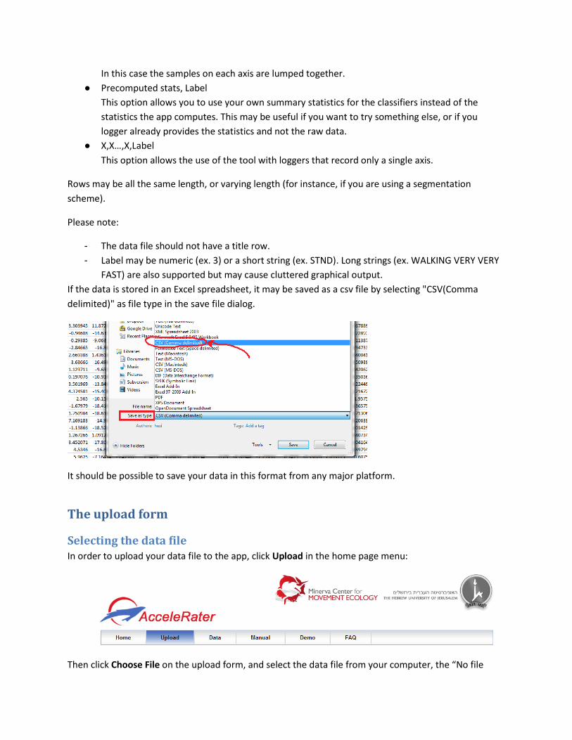
If the data is stored in an Excel spreadsheet, it may be saved as a csv file by selecting "CSV(Comma

delimited)" as file type in the save file dialog.

It should be possible to save your data in this format from any major platform.

The upload form

Selecting the data file In order to upload your data file to the app, click Upload in the home page menu:

Then click Choose File on the upload form, and select the data file from your computer, the “No file

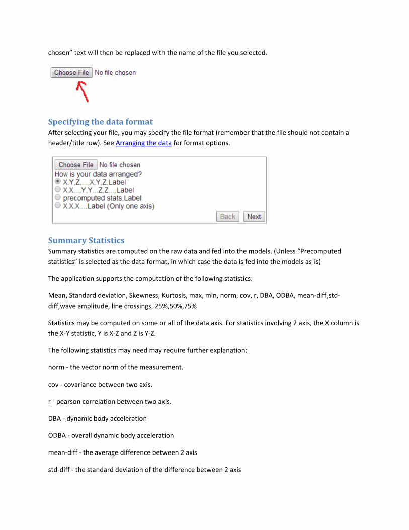
chosen” text will then be replaced with the name of the file you selected.

Specifying the data format After selecting your file, you may specify the file format (remember that the file should not contain a

header/title row). See Arranging the data for format options.

Summary Statistics Summary statistics are computed on the raw data and fed into the models. (Unless “Precomputed

statistics” is selected as the data format, in which case the data is fed into the models as-is)

The application supports the computation of the following statistics:

Mean, Standard deviation, Skewness, Kurtosis, max, min, norm, cov, r, DBA, ODBA, mean-diff,std-

diff,wave amplitude, line crossings, 25%,50%,75%

Statistics may be computed on some or all of the data axis. For statistics involving 2 axis, the X column is

the X-Y statistic, Y is X-Z and Z is Y-Z.

The following statistics may need may require further explanation:

norm - the vector norm of the measurement.

cov - covariance between two axis.

r - pearson correlation between two axis.

DBA - dynamic body acceleration

ODBA - overall dynamic body acceleration

mean-diff - the average difference between 2 axis

std-diff - the standard deviation of the difference between 2 axis

wave amplitude - the average difference between local maxima/minima

line crossings - the number of times 2 axis cross each other.

25%,50%,75% - percentiles.

Models The application supports the computation of the following models:

K nearest neighbors - This simple model labels a new sample using a vote between the K points in the

training data nearest to it. By default we set K=3, but this can be changed by the user.

Linear SVM - Linear support vector machines computer the maximum margin hyperplane between two

classes. The multi-class extension we use here computes such a hyperplane between every two classes,

and uses a vote to determine the class for a new point.

RBF kernel SVM - This model is similar to a linear SVM , but the hyperplane is computed after an implicit

projection of the data into a “much larger” space.

Decision tree- a set of hierarchical decision rules is developed that can be used to predict the class of

unclassified samples. Each rule can branch into another rule or a terminal category.

Random forest- ensemble classifiers in which sets of classification trees are constructed using a

procedure similar to a decision tree, but including introduced stochasticity . Instead of potentiall using

all the variables to determine the best split at each node, only a randomly selected subset of variables is

used.

Naïve Bayes- a simple probabilistic classifier with the strong assumption that features are conditionally

independent (conditioned on the label)

LDA- a linear model assuming Gaussian distributions with equal covariance.

QDA- the same as LDA, but without assuming equal covariance.

You may choose the models you would like to compute by checking the checkboxes in the upload form.

Alternatively, check Select all to compute all models.

Feature Selection Feature selection refers to the method of selecting the summary statistics to feed into the models. We

currently offer 3 options:

Use all features – all calculated statistics will be used.

F-test – only statistics who’s mean is significantly different between the classes will be used (with

α=0.05).

PCA – perform PCA and reduce the dimension of the statistics vector. You may choose the number of

dimensions to use.

Cross Validation The purpose of validation is to estimate how well the results of a given model will generalize to new

data. In our case, we would like an estimate of how well we can expect the classification of new ACC

data point to be. This estimate can be divided into a) overall correct classification and b) correct

classification per behavior class. Also, for a given sample from a given class, it may be of interest to know

which classes the classifier is more likely to mistakenly classify it as (This is knows as a ‘confusion

matrix’).

We offer three types of validation:

● Train-test split: The simplest (and fastest) option. The data is split into 2 parts, the first part is

used to train the models, and the second part to test the models.

● K-fold cross validation: The data is split into K equal sized partitions. On each iteration, the

models are trained on all but one partition and tested on the remaining partition. The overall

estimate is set to be the average of the K estimates obtained.

● Leave One Out – cross validation: On each iteration, the models are trained on all but one

sample, and tested on the remaining sample. The overall estimate is the percent of samples

correctly labeled.

These options offer a tradeoff between the quality of the estimate and the runtime of the calculations.

The Train-test split option may be useful for getting a first impression of the relative performance of

different models, followed be the K-fold (or LOOCV) option for further testing of a specific selected

model.

In the upload form, you may select your preferred type of cross validation.

The data and models view The data and models view will open after the data file is uploaded and the models are computed.

Computation of the models may take a few minutes, depending of the size of your data and the models

and cross validation type you selected.

The data view contains the following tabs: Raw Data, Descriptives, Models, Models summary, Behaviors

and Label new data.

Raw data

The Raw Data tab contains the first 20 rows of the data file you uploaded. The purpose of this is to verify

that the application understood the data the way you intended.

Descriptives

This tab contains some descriptive statistics that may be useful in understanding the data, the most

important of which is the number of samples in each class.

Plots with samples from each class can be requested by clicking the “Load new plots” button.

Models

The models tab includes a tabbed layout describing the computed models. Each tab refers to one of the

computed models and contains the model’s name, overall percent correct, confusion matrix both in a

tabular and graphical form, as well as tables of recall/precision and specific accuracy:

Models summary

The models summary tab displays information useful for comparison of the computed models, this

includes:

● a recall-precision plot

● overall percent correct per model. Standard deviation is computed from the cross validation

repetitions.

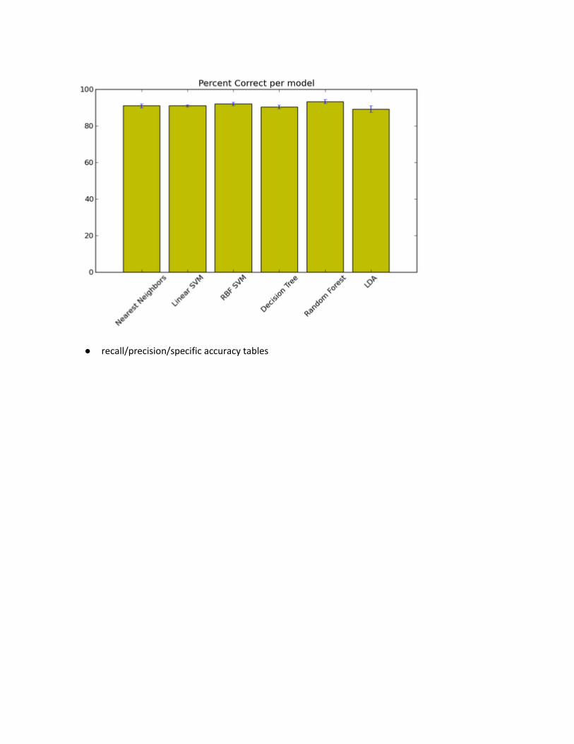
● recall/precision/specific accuracy tables

Labeling new data

It is possible to label new data with any one of the calculated models (The actual model used for the

labeling is re-trained on all the labeled data, regardless of the method of cross validation used).

In order to label new data, the samples should be arranged in a csv file in the same format as the

training data file (no Label column this time) :

See Arranging the data for more details.

After clicking "GO!" a download will begin with a csv file containing one column with the predicted

labels for your data (each row is the predicted label for the corresponding row of the unlabeled data)

Annotation of raw data on a Google-map

This feature allows the annotation of raw data on a Google-map after training a model. As of now, only

the e-obs data format is supported.

In order to display the raw data, upload an extracted logger file (text file), and select the model to use.

The trajectory will then appear on a map with color coded points, where the color represents the

behavior classification.

Downloading the calculated statistics The calculated statistics may be downloaded either in their raw form, or normalized (the way they are

later used), by clicking the download links on the top left:

The demo page The demo page contains demo files to test the app with.

The FAQ page The FAQ page is a list of common questions regarding the app and our answers. If you have additional

questions, please see next section for contact information.

Contact us email: yehezkel.resheff@mail.huji.ac.il

address:

Yehezkel Resheff

The movement Ecology Lab

Room 101, Berman Bldg

The Hebrew University of Jerusalem, Edmond J. Safra Campus at Givat Ram,

Jerusalem 91904, Israel