BEACH DYNAMICS OF KERALA COAST IN RELATION TO LAND-SEA INTERACTION

Thesis submitted to the

COCHIN UNIVERSITY OF SCIENCE & TECHNOLOGY for the degree of

DOCTOR OF PHILOSOPHY IN

PHYSICAL OCEANOGRAPHY

By

R. SAJEEV, M.Se

NATIONAL INSTITUTE OF OCEANOGRAPHY REGIONAL CENTRE

COCHIN - 682018

DECEMBER 1993

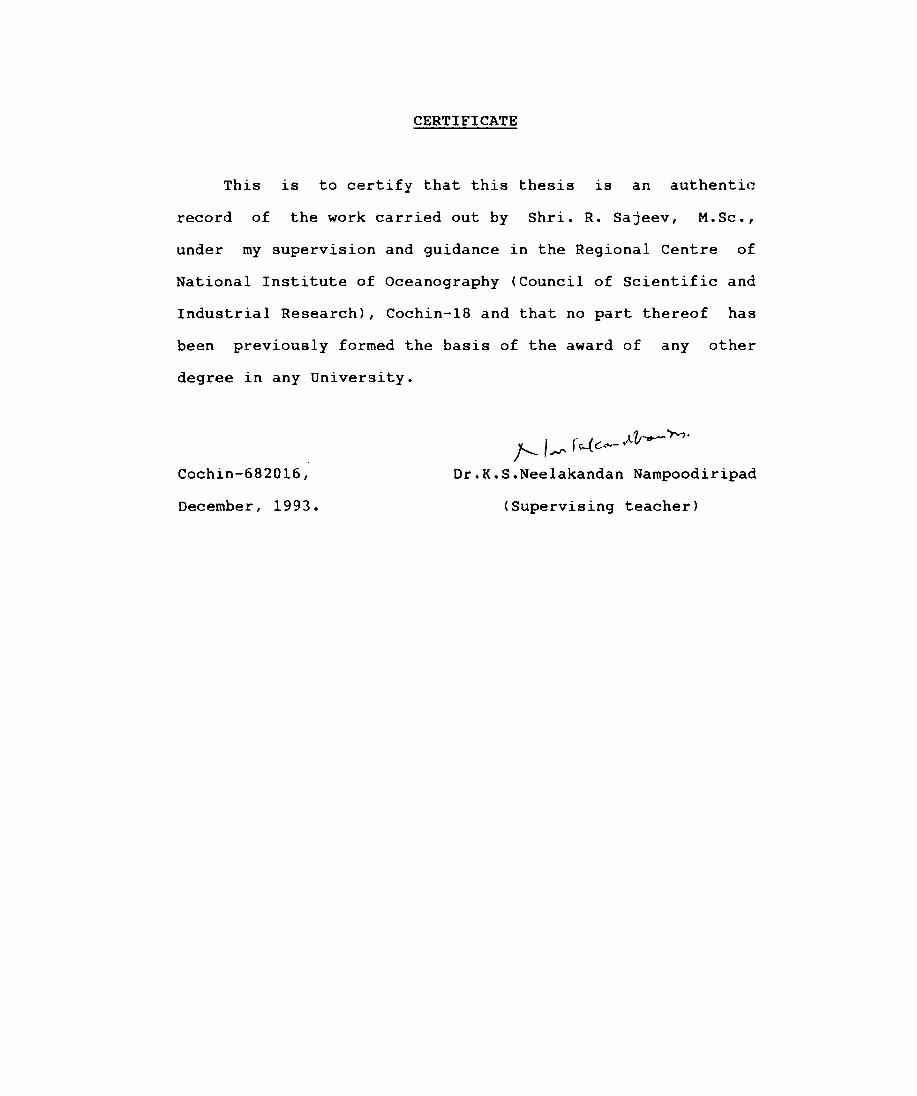
CERTIFICATE

This is to certify that this thesis is an authentic

record of the work carried out by Shri. R. Sajeev, M.Sc.,

under my supervision and guidance in the Regional Centre of

National Institute of Oceanography (Council of Scientific and

Industrial Research), Cochin-18 and that no part thereof has

been previously formed the basis of the award of any other

degree in any University.

Cochin-682016,

December, 1993.

J-,~r~v-~~~' Dr.K.S.Neelakandan Nampoodiripad

(Supervising teacher)

CONTENTS

ACKNOWLEDGEMENTS

PREAMBLE

CHAPTER 1.

1.1.

1. 2.

1.2.1.

1.2.2.

1.2.3.

1. 3.

1.4.

1. 5.

CHAPTER 2.

2.1.

2.2.

2.2.1.

2.2.2.

2.2.3.

2.2.4.

2.2.5.

2.3.

2.3.1.

2.3.2.

2.3.3.

INTRODUCTION

Coastal geomorphology of India

Description of the Kerala coast

Morphological features

Physical factors

Man made structures

Scope of the present work

Area of investigation

Previous studies

WAVES AND WAVE TRANSFORMATION

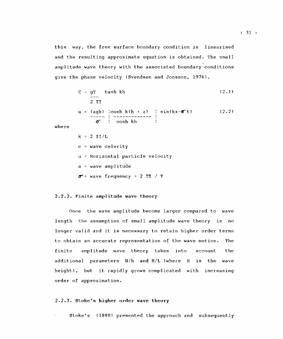
Wave climate

Wave theories

Small amplitude wave theory

Finite amplitude wave theory

Stoke's higher order wave theory

Cnoidal wave theory

Solitary wave theory

Wave transformation

Shoaling

Refraction

Numerical wave refraction

• • • • • •• v

· . . . . .. vi

• . . . • •• 1

· · · · · · . 1

· · · · · · · 2

· · · · · · · 5

· · · · · · · 6

· · · . · · · 11

· · · · · . · 11

· · · · · · · 13

· · · · · · · 14

· ...... 26

· . . . . . . 26

· . . . . . . 29

· . . . . . . 30

· . . . . . . 31

· ...... 31

· . . . . . . 32

· . . . . . . 33

· . . . . . . 34

· . . . . . . 35

· ...... 36

· . . . . . . 39

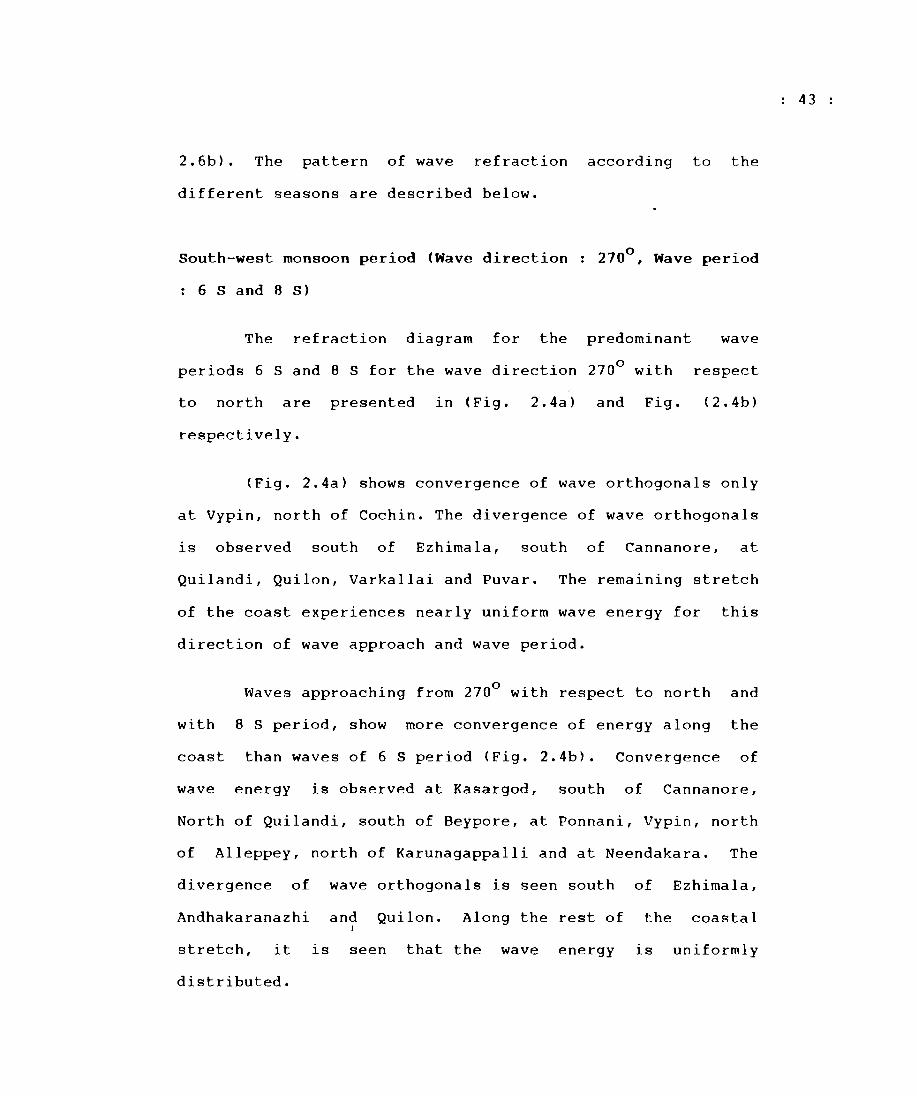
2.4.

2.4.1.

2.5.

2.5.1.

Construction of refraction diagram

Input for the model

Results

Variation of breaker parameters

CHAPTER 3. BEACH DYNAMICS

3.1. Beach morphology

3.1.1. Materials and methods

3.1.2. Results

3.2. Beach sediments

3.2.1. Materials and methods

3.2.2. Results

CHAPTER 4. SEDIMENT TRANSPORT

4.1. Littoral environmental observation

4.1.1. Materials and methods

4.1.2. Results

4.2. Longshore sediment transport

4.2.1. Materials and methods

4.2.2. Results

CHAPTER 5. SUMMARY AND CONCLUSIONS

SCOPE FOR FUTURE STUDY

REFERENCES

APPENDIX-I

· . . . . . . 40

· ...... 41

· ...... 42

· . . . . . . 45

· . . . . .. 51

· ...... 51

· . . . . . . 51

· ...... 54

· ...... 68

· . . . . . . 69

· . . . . . . 70

· . . . . . . 76

· ...... 76

· . . . . . . 76

· . . . . . . 77

· ...... 80

· . . . . . . 82

· ...... 86

· ...... 91

· ...... 103

· . . . . .. 104

· . . . . .. 122

PREAMBLE

" What sight is more beautiful than a high energy beach

facing lines of rolling white breakers? What battle

ground is more ferocious than where waves and sand

meet? What environment could be more exciting to

study than this sandy interface below land and sea?

And yet how much do we know about sandy beaches?"

••••••.• McLachlan and Erasmus (1983)

Coastal zones are recently receiving increased

attention of the scientific and engineering community. This

interest is motivated from the thrust and pressure of the

economic development which demands a better understanding and

utilization of the coastal belt, as it accommodates more than

sixty percent of the world's population. The expansion of

world trade demands construction of a large number of

harbors and terminals. The varied human interference on the

coastal zone also includes exploitation of living and non

living marine resources, recreation, navigation, waste

disposal, etc .•

The sandy portion of the coastal zone, the beach, is a

complex and dynamic ~nvironment which is examined in detail

in this thesis. The general configuration of a beach changes

continuously, in response to the variations in the forcing

functions like winds, waves, currents and tides etc. in

addition to the man-made changes.

vi

The beaches

topographic changes

varying monsoonal

of Kerala coast undergo

under the influence of the

forcing. At times, the

considerable

seasonally

beach sand

containing valuable minerals is lost in large quantities due

to erosion which are local and seasonal. It is in thiR

context that studies on problems of the coastal and nearshore

areas along the coast of Kerala received considerable impetus

in recent years. There had been a number of studies in the

past, concerning various aspects of beach/coastal dynamicR

along the different stretches of the coast of Kerala.

However, efforts to study Kerala coast as a whole combining

both the theoretical model and comprehensive field

observation have been lacking_ Hence the problem " Beach

dynamics of Kerala coast in relation to land-sea interaction"

has been taken up for this doctoral thesis. The result of

this study could. provide the basic information much needed

for the planning of various developmental projects so as to

achieve sustainable economic growth of the hinder land.

~ue to variations in the nature and type of the

beaches constituting the Kerala coast, the responses of the

individual beaches are different, though the monsoonal

forcing is more or less same. In view of this, 8 sites were

selected at various locations with Kasargod in the north to

Trivandrum in the south, along the entire stretch of the

Kerala coast for the field observations, taking into account

Lhe morphological setting. The field observations consisted

of detailed survey on waves, littoral currents and beach

vii

characteristics for a period of one year from March 1990 to

February 1991.

The thesis is addressed in 5 chapters. The first

chapter provides a general introduction to the topic,

geomorphological settings of India and Kerala with factors

affecting the stability of the coast. The locations of study,

aim of the present work, research approach, and a review of

literature on the various coastal processes are also included

in this chapter.

Chapter two deals with the wave theories, wave climate

along the region under study, wave transformation model used

and the results of the model has been presented.

Third chapter highlights the results of the field

studies on beach morphology and grain size composition of

beach material. The results arrived at from the application

of E.O.F analysis have also been presented in this chapter.

The.results of the Littoral Environmental Observation

(L.E.O) and the sediment transport estimations for the Kerala

coast are discussed in the fourth chapter.

The last chapter synthesizes the results obtained in

the earlier chapters to arrive at a comprehensive picture of

the beach dynamics of the Kerala coast. It is followed by a

list of references cited in the text. The computer program

used for the construction of refraction diagram is given as

Appendix-I.

viii

CHAPTER 1

1. INTRODUCTION

The zone where land and sea meet is a complex

environment. The coastal areas of the world are of extreme

economic importance as approximately, two-thirds of the

world's population live along the 4,48,000 km coastlines. In

ntust of the highly developed countries, industrial,

residential and recreational developments as well as large

urban complexes occupy much of the coastal margin. The future

expansion in many undeveloped maritime countries will also be

concentrated on coastal areas. Inorde~ to utilize the coastal

zone to the maximum of its capacity, and yet not plunder its

resources, an extensive knowledge of this complex environment

is necessary for geologists, engineers, oceanographers and

coastal planners engaged in the coastal zone management. The

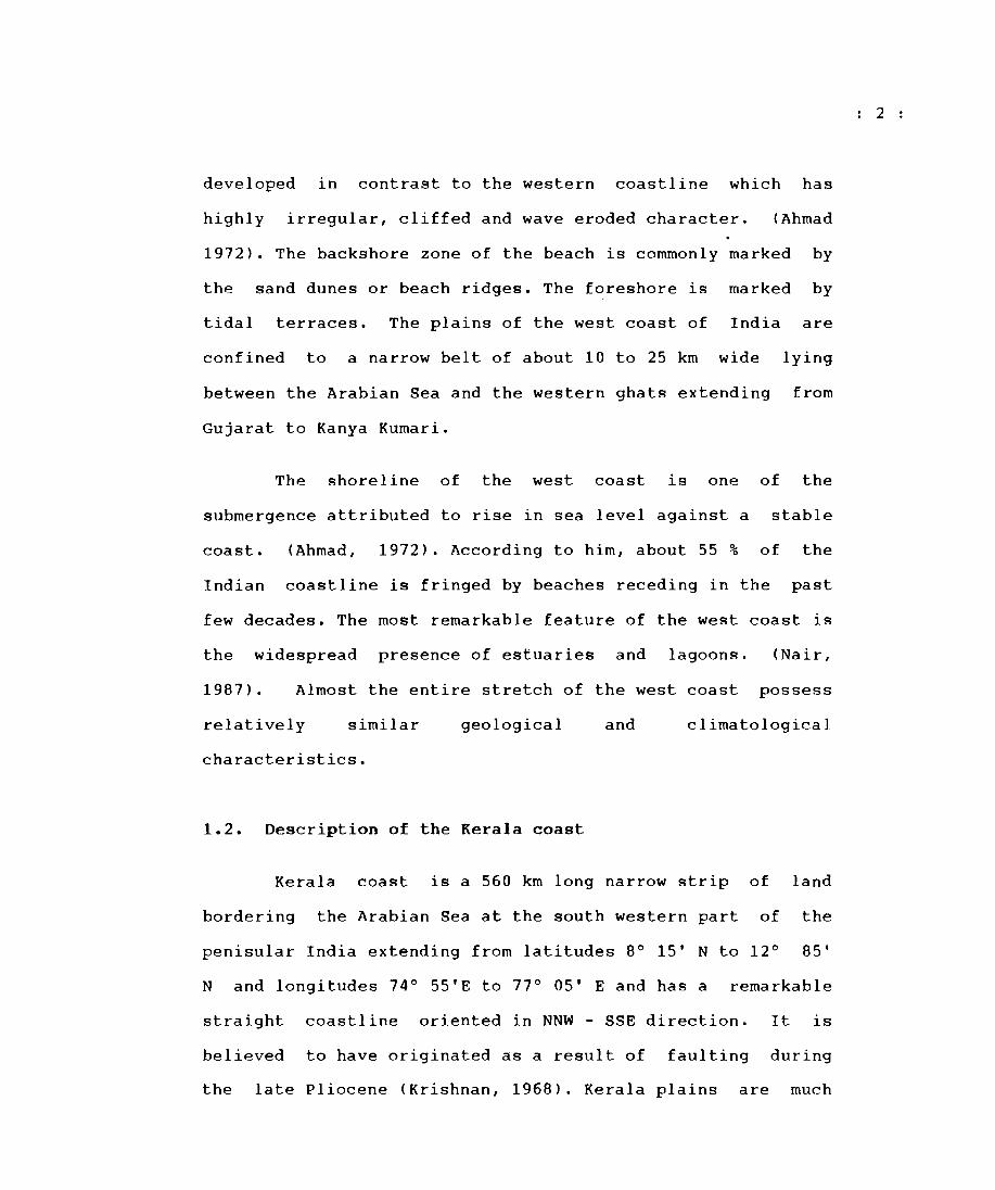
general configuration of the beach (Pig. 1.1), changes

continuously in response to the time varying forcing

functions viz. winds, waves, currents, tides etc •.

1.1. Coastal geomorpho!ogy of India

India has a long coastline of about 6500 km. The

shelf has a gentle uniform gradient. Cliffs and offshore

islands are comparatively scarce, while barriers and spits

are common. The coastline of India is characterised by

varieties of features like rocky headlands, coral reefs,

reef-like structures, tidal inlets, estuaries, lagoons,

barrier islands, bays,

essentially alluvial,

etc.

gently

The eastern

indented and

coastline is

extensively

1

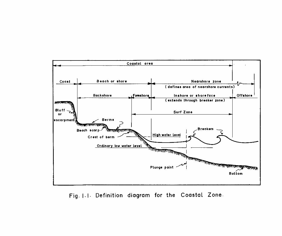
Coast

Bluff or

Coa.tal area

Beach or .hore Nearshore zone

( defines area of nearshore currents)

Back.hore fo .... hor. Inshore or .horeface Offshore ( extends throuQh breaker zone)

Surf Zone

Crest of berm High water Level

Breakers ~

~ .,.-

Ordinary low water Level

PLunQe point ~~"'&'fM"""+4tawu. Bottom

Fig. I· I· Definition diagram for the CoastaL Zone.

developed in contrast to the western coastline which has

highly irregular, cliffed and wave eroded character. (Ahmad

1972). The backshore zone of the beach is commonly marked by

the sand dunes or beach ridges. The foreshore is marked by

tidal terraces. The plains of the west coast of India are

confined to a narrow belt of about 10 to 25 km wide lying

between the Arabian Sea and the western ghats extending from

Gujarat to Kanya Kumari.

The shoreline of the west coast is one

submergence attributed to rise in sea level against a

coast. (Ahmad, 1972). According to him, about 55 %

of the

stable

of the

Indian coastline is fringed by beaches receding in the past

few decades. The most remarkable feature of the west coast is

the widespread presence of estuaries and lagoons. (Nair,

1987). Almost the entire stretch of the west coast possess

relatively similar geological and climatological

characteristics.

1.2. Description of the Kerala coast

Kerala coast is a 560 km long narrow strip of land

bordering the Arabian Sea at the south western part of the

penisular India extending from latitudes 8° 15' N to 12° 85'

Nand longitudes 74° 55'E to 77° 05' E and has a remarkable

straight coastline oriented in NNW - SSE direction. It is

believed to have originated as a result of faulting during

the late Pliocene (Krishnan, 1968). Kerala plains are much

2

wider and less hilly than the rest of the west coast. Recent

observations indicate that the shoreline as a whole is

dynamic and neotectonically active leading to considerable

erosion and loss of surface area. Narrow stretches of sandy

beaches are present all along the coastline except in areaR

of cliffs.

The elevation of the shoreline on the western side

bordering Arabian sea ranges from 0 - 5 m. Intervening the

ghats and the shoreline are exposures of tertiary formations

such as the Miocene Warkalli at Varkala in south and

Tellicherry-Cannanore in the north. North of Varkala for

about 100 km there are coastal Tertiaries occupying the zone

between the extremely narrow alluvial bars towards the shore

and the edges of the gneisses and granites interior on ,the

east. This consists of marine fossiliferous coral line

limestones and sands and clays with bands of lignite. They

ar~ frequently capped by laterite. The present shoreline is

straight for over a great part of the length from Calicut to

Quilon, but in Cannanore, Trivandrum and Quilon districts,

indentations, cliffs and protuberances are present.

The width of the continental shelf along the Kerala

coast varies widely from south to north. Major contributions

for the shelf deposits are the west flowing rivers. There are

44 rivers flowing west into the Arabian sea which originate

from the hills of the western ghats and drain into the

backwaters.

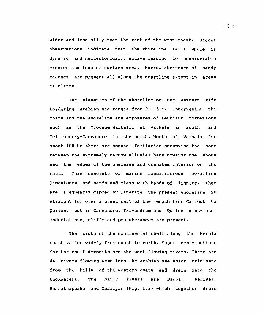
Bharathapuzha

The major rivers are Pamba, Periyar,

and Chaliyar (Fig. 1.2) which together drain

3

~ ________ ~~~ _____________________ 1~~ _____________________ 7~~~' ______________ .~

1. Valapatanam R,

'7

CANI'IANNO RE

'7

CAUCUT

2 .Chaliyar R.

J.8harathapuznd R·

4 . periyar R.

COC HIN

~ S.MUVdtt u pUZha R.

'7 5.Me~nachil R.

7 · Vem banddtJ LdKe ALLEPP E Y

8. Manimala R. <;). Pdmbd R.

10.Achdncoil q.

11 . Kdlld da R. LEGEND.

12. AShtamud i U K e ~UI i_ON

Mid Land - 0 ·7 5 M

T

\ , '- - '-

I:···.::·:: : .] Law Ldnd - Beta ... ' · 8 M fRIVAN 0 RUM

source' SCST , 1'382 .

"" 'f..

'" )v

'- . 'J

'7

Fig. 1.2. Physiography and major rivers of Kerala

"\ .-.1t

I ./

" ) '-' '

., 10

z

>

o

c

35% of the state's average discharge. The rivers of Kerala

swell up during monsoon season into gushing torrents and

shrinks into modest dimensions during summer months. They

6 3 carry 45060 X 10 m of water per year (Anonymous, 1974). The

dams constructed across many of these rivers for power

generation and irrigation have considerable influence on the

sediment budget of the coastal zone.

The beaches of Kerala are composed of fine to coarse

grade sands (0.15 to 0.50 mm). The coastal area is mostly of

sub-recent to recent sediments. The structure of the coast

from Quilon to Quilandy have alluvial belt covered by

laterite deposits. Placer deposits of considerable economic

importance are present along the beaches of Kerala. The

concentration of the heavy minerals like Ilmenite, Monozite,

Rutile and Zircon in the coastal area from Neendakara to

Kayamkulam is an important feature of the coast. Apart from

various shades, the beach material comprises of shell

fragments, magnetite, sillimanite and rare earths. The placer

deposits of Kerala's coastal stretch occupies a pride place

in India.

Muddy bottom shelf extends 50 to 60 kms from the coast

to a depth of lOOm. Beyond this, the shelf slopes down

steeply to 1000m. The bathymetry of the inner continental

shelf and nearshore of the south-west coast show considerable

variability along its length. The slope of the continental

shelf decreases towards north and increases north of

Cannanore. (Baba, 1988).

4

5

The coastal zone of Kerala is well known for its rich

fisheries, placer mineral deposits, water resources, .

transport facilities, excellent backwater systems and above

all a well literate and hard working popUlation. It is also

rich with wetlands having mangroves, industries, ports and

harbors, tourism and recreational facilities.

1.2.1. Morphological features

Lagoons and estuaries

Along the Kerala coast, between Quilon and Kasargod,

long and irregular lagoons are present behind the impressive

coastal barriers. Many of the lagoons, locally known as

Kayals, are bestowed with numerous islands of different

sizes. There are 34 Kayals in this area. Among these lagoons,

Vembanad lake is the largest (205 sq.km) followed by

Ashtamudi Kayal further south. The Vembanad lake opens into

the Arabian Sea at Cochin. Six major rivers, Periyar, Pamba,

Manimala, Achankovil, Meenachil and Muvattupuzha discharge

into this lake. Lagoons and estuaries play an important role

in beach dynamics along this coast.

Bars, spits, headlands and barriers

The south-west coast, as a whole, is well known for

most well-developed bars and lagoons. Low cliffs alternating

with pocket beaches, promontories, head-lands and bays are

present along the coast of Kerala. North of Ponnani, the

shore consists of continuous formation of mainland beaches.

North of Trivandrum, the coast is characterised by the

presence of barrier beaches except at few places where. rocky

cliffs and head lands are present. Where the lagoons opens

out into the sea across the bars, spits are present with or

without submerged sand bars.

The principal influence of the lagoolls in-sa-far as

beach studies are concerned is that they act as sediment

traps. A well developed barrier is seen between Neeleswar and

Cannanore. The Vypeen Island barrier, north of Cochin, is

about 23 km long and 2 km wide. Several barriers are observed

near Quilon. Remarkable features of the barriers are their

alongated formation with small width.

1.2.2. Physical factors

Climatology of Kerala

.Orographic influence on the monsoons plays an

important role in the climate of Kerala. In the

meteorological map of India, Kerala has a pre-eminent place.

It is the gateway through which great rain-bearing south-west

monsoon current gains access to the subcontinent year after

year by the end of Mayor in early June and through which the

monsoon make its lingering exit towards the end of the year

after having dispersed its priceless bounty over the length

and breadth of the country <Ananthakrishnan et al., 1979).

Av(~r,\ge a.nnua.l rainfall in Kerala is nearly 300 cm, which is

6

-11

-10

9-

76- 77°

'-<".,. SOUTH-WEST MONSOON (June-Septl 'r-. (.r) (1901-79)

r '''1 ....

\. \ .....

'''\.-\. ~12' '. ,.,

CANNANORE" \\ l~·.· l .... \..,.

MAH~ \ ~ "'. /"(

KOZHIKODE

11-

-10

tJ

7~- - 76- 77·

-12

I i

101

tJ

7~-

76- 77-

NORTH-EAST MONSOON (Oct -Dec.) ( 1901-79)

76-

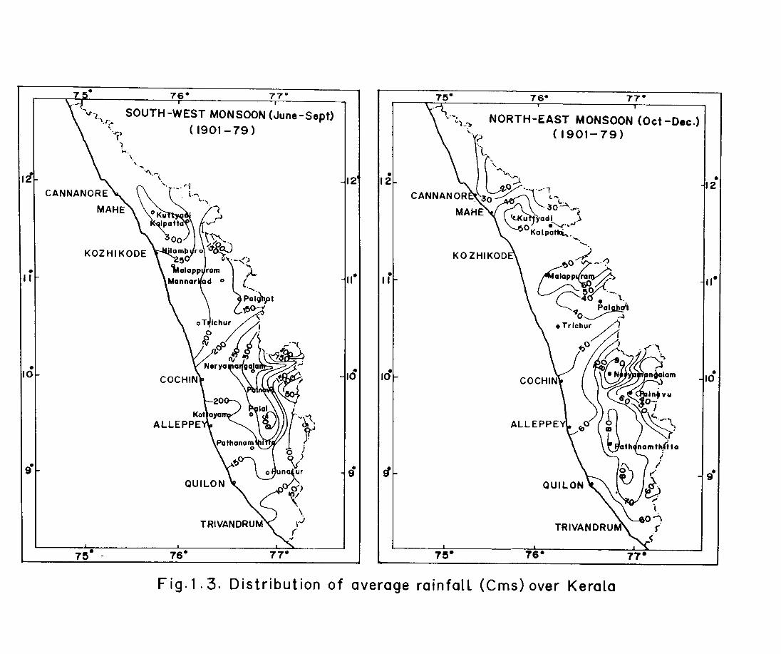
Fig.l .3. Distribution of average rainfall (ems) over Kerala

-12

11-

-10

9-

about three times the average annual rainfall of India. The

distribution of average rainfall over Kerala state during the

south-west monsoon (June-September) and north-east monsoon

(October-December) are shown in Fig. 1.3.

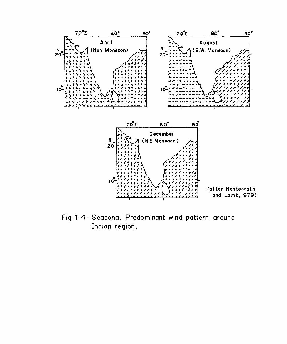
Wind

The basic feature of wind distribution over Arabian

Sea is the reversal of the wind systems during an year known

as the monsoon. The reversals take plac~ predominantly from

south-west direction during May-September to north-east

direction during December-March. Between these reversals are

the transition periods during which weak and variable winds

prevail. The typical wind pattern for different seasons

(south-west monsoon, north-east ·monsoon and non-monsoon

seasons) are shown in Fig. 1.4. The wind set up caused by

wind pushing surface water against the shoreline results in a

change of the existing equilibrium profile of the beach. The

.wind is also significant on a wide sandy beach as largn

quantities of sand can be blown from the beach.

Tides

The tide is an important factor influencing the beach

dynamics. Tidal currents which are oscillatory in nature are

particularly important in transporting sand in shoals and in

the formation of sand waves on submerged bars around

entrances to bays and estuaries~ but have virtually no effect

on uninterrupted straight shorelines, except in areas with

7

April

(Non Monsoon) 4~~~ ~f~ "~~~, ~~~

\\""~'" 1I1~,f1 _"""'ll~~ ,-"111 11 ,,.-.. le , It'll" ..... .,. 11 ~ "If 1" JI

lr~"lc"'II:'" +t11'11lf'JI

~""II"II"'Io tof""'''''''.' ~~ ... ~"\'-,, .. t+ ..... ttttt ~ • \ lc " le ..... " '" if' It ,,~~ ... " " .. • • \1."""""" tltlt~II-':'"",,,,,, '.~~'4"\i"~!S ""~IO(~" ..... , .. ~~~~\~~~~~ ri~~~'~l'f~ ~\~\\~"~~ ~ .. ~~tt~n~, ""'''_'» ... ; ... , ........ -:t~ 1'''' tto.",. .. ~\ '\ ....... .". .,.~ .... '~~1::' 1'7J? 1. t f 4 ".~ ~'II .... "lo~~ ...... ,~ .?r-" ,,""

8 •

December N. 20

( NE Monsoon )

8 •

August

(S.W. Monsoon)

• 90

(after .Hastenrat h and Lamb,1979)

Fig. 1· 4· Seasonal Predominant wind pattern around Indian region.

very large tidal ranges. The tides of Kerala are mixed,

semidiurnal in nature and occur within the microtidal range

«2m).

Nearshore waves

Most of the dynamic nature of the beach and nearshore

zone is the direct or indirect result of wave action. Wave

information is vital in design and construction of various

coastal and offshore structures, ports, harbors and for

various ocean engineering projects. For an understanding of

long term variability of beaches, and for variouR

developmental activities of the coastal region, wave data is

very much essential. Energy mainly from wind, imparted to the

water produces wave motion and are modified by the general

configuration and contour of the near shelf. Waves are the

most important cause of alteration and evolution of our

coastlines. During south-west monsoon, due to the strong wind

action, increase in wave activity with long swells and high

breakers has been observed along the Kerala coast Considering

the orientation of the coastline (NNE - SSW), wave directions

varying between 1800 - 3400 are more significant in the shore

processes. In the south-west monsoon season the predominant

direction of waves fall between WSW and WNW.

Longshore currents and rip currents

One of the major effects of wave action in the shallow

water is the generation of longshore current, which plays an

8

important part in the longshore movement of material. As the

waves arrive obliquely to a straight coastline and break at

an angle to the beach, they generate longshore current

flowing parallel to the shoreline. This wave induced current

is confined to the nearshore, rapidly decreasing in velocity

beyond the breaker zone. The nearshore currents varying in

space and time are responsible for many of the beach

processes.

Rip currents are the most noticeable of the exchange

mechanisms

strong and

between offshore and surfzone. Rip currents arn

relatively narrow jets of seaward flowing

currents. The rips are fed by a system of longshore currents.

Bowen (1969) has shown that cell circulation with rip

currents is produced by longshore variation in the wave

breaker heights.

Littoral transport

The longshore current transports beach sediments for

many kilometers in the longshore direction. Littoral

transport of sand occurs in two modes. 1) parallel to the

shoreline due mainly to the effect of longshore current,

which is referred to as longshore transport

perpendicular to the shoreline due to swash and

referred to as the beach drift.

and 2)

backwash,

The direction of longshore transport varies from

season to season, day to day or hour to hour depending upon

9

the location and direction of the storm winds which generate

waves. It results from the stirring-up of the sediments by

breaking waves and movement of sediment by the lon9shore

component of wave induced current. The beach drift occurs as

a result of the stirring up of the bottom sediments in

breaker zone which tend to be carried up the beach to the

limit of swash of the breaking wave and back with back wash.

The volume of the beach drift is determined primarily by wave

steepness, sediment size and beach slope. Determination of

the amount of sand that can be moved in the onshore-offshore

mode is difficult and entails detailed profile surveys.

Mud banks

Mud bank is a phenomenon peculiar to the south-west

coast of India. The occurrence of mud banks provides safe and

smooth anchorage even during the rough wave conditions of the

south-west monsoon. As many as 27 locations are identified

where mud banks had appeared along the Kerala coast. This

has been classified into three regions, viz. the southern

strip (Thrikkunnapuzha. - Alleppey),. the central strip

(Chellanum-Munambam) and the northern strip (Calicut pier­

Muzhappilangadi) by Nair (1983). The mud banks are reported

to be decisively affecting the equilibrium conditions thereby

causing shoreline instability of the coast. They trap the

littoral materials from either side thereby preventing it's

downdrift, causing accretion within the mud banks and erosion

on down drift sides.

10

1.2.3. Man made structures

Apart from natural phenomenon, the man-made structures

along the coastline act as barriers to the material' and

energy balance, and produce adverse effects on the stability

of the nearby coast. Kerala's maritime activity is mainly

related to the major port at Cochin. There are 3 intermediate

ports and 11 minor ports along this coast. Some of the man­

made barriers are dredged channels, jetties, groins, sea

walls and break waters. The structures constructed along

these ports have triggered many environmental problems in

addition to upsetting the sand balance in many locations of

the coastal zone.

1.3. Scope of the present work

The sandy portion of the coastal zone is a complex and

dynamic environment which is investigated in detail in this

thesis. The general configuration of the beach changes

continuously, in response to the variations in

functions namely winds, waves, currents and

the

tides

similar time scale as these forcing mechanisms. The

work is aimed at a theoretical and field assessment

forcing

on a

present

of the

physical processes involved in the shoreline development and

beach stability along the entire stretch of the Kerala coast

from Kasargod in the north to Trivandrum in the south.

Along the Kerala coast, the beaches are subjected to

changes of varying degrees in response to seasonally varying

11

12

monsoonal forcing. At times, the beach sand containing

valuable minerals is lost due to erosion which may be local

or seasonal. It is from this view point that studies on .

problems of the coastal and nearshore areas along the coast

of Kerala received considerable impetus in recent years.

There had been many studies in the past, concerning various

aspects of beach/coastal dynamics along the different

stretches of the coast of Kerala. However, studies along the

entire stretch of the coast of Kerala combining both the

theoretical model and field observations are practically

lacking. It is in this background that the problem "Beach

dynamics of Kerala coast in relation to land-sea interaction"

has been taken up in this study. The present study aims at

examining 1) the dynamic response and stability of different

types of the beaches along the coast of Kerala, 2) the

predictability of the beach changes along the entire stretch

of the Kerala coast, both theoretically and empirically. The

result of this study could provide the basic information

required for various developmental as well as recreational

purposes.

The objectives of the present study are achieved through

following :

1) The application of a numerical wave transformation model

for the Kerala coast to study the distribution of

nearshore wave energy for the predominant deep water wave

directions and periods.

2) The application of the Empirical Orthogonal Function

(E.O.F) analysis to the beach morphology and grain size

data to separate the temporal and spatial variations and

thereby relate the E.O.F mode of beach morphology and

grain size to the waves.

3) The study of the variations in grain size of beach

sediments from Kasargod to Trivandrum and to bring out

the physical factors controlling different environments

of the beach.

4) The estimation of the longshore sediment transport based

on the field observation. (LEO data Littoral

Environmental Observation data).

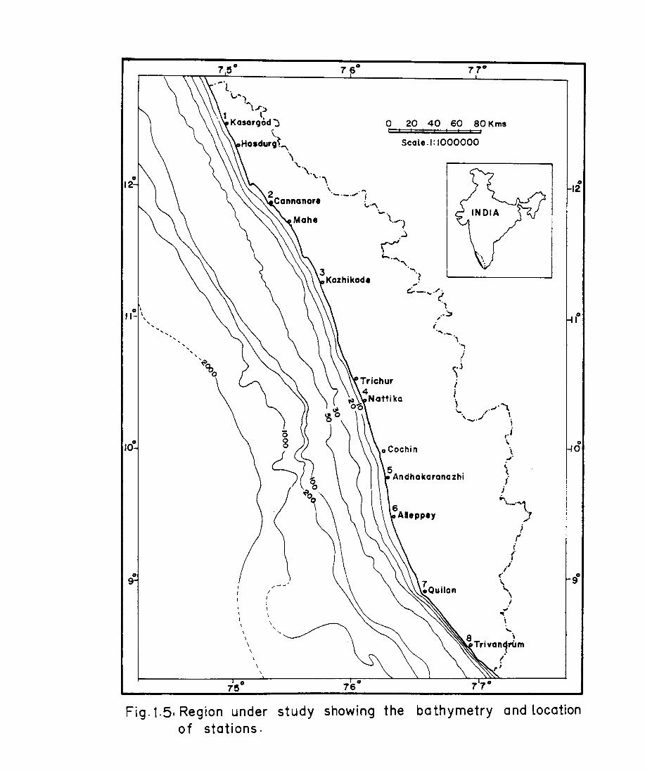
1.4. Area of Investigation

The field observations consist of a detailed survey on

waves, littoral currents, beach sediment size and beach

morphology for a period of one year along the Kerala coast

from Kasargod (Lat. 12° 13'N and Long. 74° 58' 24"E) to

Trivandrum (Lat. 08° 29' 11"N and Long. 76° 54' 12' 'E),

consisting beaches of different morphologic types.

Due to the geographical variations of the nature and

type of beaches constituting the Kerala coast, the responses

of the individual type of beaches is different, though the

monsoonal forcing is more or less same. Inview of this, 8

sites were selected along the entire stretch of the kerala

coast (Fig. 1.5) for the field observation by taking into

13

0'

11- " ... ,~

o 9

~ ... , ... ,

... ... ... , '~ Cbo

\

\

\

\

I I , I \

\

o ,

...

20 40 60 80 Kms , , , , , , ,

Scale.l: 1000000

i i ) -,.~ ..... ." \ '_ . ./ i

,.i \,

\ i

j .... ~""1

) ! ,.

i (

,.i ('

" , \ .I .,

'" i ....

eT' d ~ 'Ivan1rtlm /

,j

o 12

o o

Fig. 1.5. Region under study showing the ba thymetry and Location of stations.

account the morphological settings. They have been chosen to

represent headland beaches, barrier beaches, open coast

beaches, beaches exposed to low and high energy environment

and beaches in the vicinity of mud bank formation.

1.5. Previous Studies

Much work has been done in India and elsewhere on

various types of coastal process phenomena.

A good deal of literature have been generated in

regard to the general principles, beach set up, various

processes and structure of the beaches (Bascom, 1954, 1980;

Inman and Fratuschy, 1966; Ippen, 1966; Romar and Inman,

1970; Ring, 1972; Shepard, 1973; Ro~ar, 1976; Goldsmith et

al., 1977; Curt, 1990; Wiel, 1991). They have conducted

various experimental as well as model studies on this

subject. The Coastal Erosion Board (CEB), Army Crops and thp. ./j/-

CERC (Coastal Engineering Research Centre) of United states

have made substantial contributions on beach processes and

configuration. The stability of beaches in California and

north Carolina have been extensively described by DingIer

(1981) and Dolan (1965) respectively. Beach processes and

erosion in various beaches of United states have been studied

by Brunn (1954), Caldwell (1956), Giles and Pilkey (1965) and

Ingle (1966).

The first attempt to quantify the longshore sediment

transport of sand has been made by Scripp's Institution of

14

Oceanography. Many theories have been developed using the

relationship between the wave forces and the transport of

sediment (Krumbien, 1944; Savelle, 1950; Johnson, 1956;

Galvin, 1972; Komar and Inman, 1970; Komar, 1976; Walton and

Bruno, 1989). Extensive studies on nearshore currents have

been made over the last several years. Several investigations

have been made both in the field and laboratory to obtain a

quantitative measure of the field of motion in relation to

the breaker characteristics utilizing the concept of

radiation stress. (Longuet-Higgins and Stewart, 1962). Many

theories have been initiated to derive the nature of

circulation in the surf zone (Bowen, 1969;· Inman and Bagnold,

1963); Sonu, 1972; Noda, 1974). All these studies have shown

the occurrence of descrete circulation cells for normal

incidence of wave rays. Sediment drift estimations based on

empirical relationship developed from quantitative estimates

of littoral flows through wave refraction studies and field

experiments have been made along various coastlines of the

world. Pyokari and Lehtovaara (1993) have studied the beach

material and its transport in accordance with the predominant

wave directions on some shores in Northern Greece. Bagnold

(1963) and Horikowa (1978) have conducted model experiments

and explained the formation of beaches. Friedman (1967) has

given a detailed picture of dynamic processes and statistical

parameters and compared the size frequency distribution of

beach and river sands. These studies, both experimental and

theoretical, have brought out the importance of topography

15

and radiation stress in the realistic derivation of the

complicated field of motion within the surfzone.

Earlier studies of the morphology of sandr beaches,

for example those reported by Eliot (1974), Wright et al.

(1978, 1979), Chappel and Eliot (1979), Short (1979), Short

and Wright (1981) and Frew et al. (1983) have described a

morphologic patterns and highlighted their variety of

susceptibility to changes. Previous statistical analyses of

beach profile data have been stochastic in nature or have

treated the changes in profile configuration as Markov

processes (Sonu and Young, 1970; Sonu and Van Beek, 1971;

Sonu and James, 1973). The E.O.F method has been applied for

morphological studies of the beaches at Torrey Pines in

United states (Winant et al., 1975; Aubrey, 1979; Aubrey et

al., 1976), at Gorlestone and Great Yarmouth (Aranuvachapun

and Johnson, 1979) and at Coledale (Clarke et al., 1984) and

for prediction of beach changes at Torrey Pines (Aubrey,

1978) •

studies on different coastal processes relating to the

east and west coasts of India are briefly reviewed in the

following sections.

East coast of India

Detailed coastal geomorphological studies have been

carried out first by Andhra University (1954 and 1958), along

the east coast of India. In addition, littoral processes

16

along the east coast have been investigated by La Fond and

Prasada Rao (1956), Sastry (1958), Subba Rao and Madhusudhana

Rao (1970), Varadarajulu (1972), Reddy et al. (1979),

Chandramohan et 'al. (1981), Vasudev (1982), Chandramohan and

Narasimha Rao (1984), Chandramohan and Rao (1985) and Sundar

and Sarma (1992). Wave refraction studies using graphical

method has been carried out by Prasad et al. (1981) and

Uhanalakshmi (1982). Sediment dynamics along the east coast

has been studied at Kakinada Bay by Subba Rao (1967) and at

Madras and Puri by Kanth (1984). Grain size trends in the

Kakinada beach have been studied by Sathyaprasad et al.

(1987). Other studies relate to analysis and hindcasting of

wave data along the coast. (Sathe et al., 1979; Reddy et al.,

1980; Mukherji and Sivaramakrishnan, 1982a, 1982b).

Chandramohan et al. (1991) compared reported wave data with

instrumentally measured waves at Kakinada coast.

West coast of India

Since coastal processes along the west coast have been

investigated by

aspects of the

many researchers in ~elation to

beach problems, they have been

classified subjectwise herein.

various

broadly

Geomorpholo9Y : Formation of the Kerala coast with it's net­

work of lagoons and estuaries and rich and heavy mineral

sands has been studied by Prabhakara Rao (1968). Studies on

the origin and distribution of black sand concentration on

the southern coast of India have been carried out by

17

18

Aswathanarayana (1964). Later, Jacob (1976) described the

general geology of south Kerala including the structure,

tectonics and erosion. Soman (1980), Thiagarajan (1980) have .

reviewed the earlier studies on geology and geomorphology of

Kerala.

studies on morphological changes at selected places

along the west coast of India in relation to wave energy have

been made by Veerayya (1972), Veerayya and Varadachari (1975)

and Murty (1977). The coastal evolution of Kerala with

special reference to coastal instability and erosion has been

reviewed by Varadarajan and Balakrishnan (1980). Coastal

geomorphology of Kerala has been described by Nair (1985).

Report by Kerala Engineering Research Institute, KERI (1971)

shows that 600 m wide belt of land has been lost during a

period of 120 years from 1850 to 1970. Shoreline changes

based on historical records have been investigated by

Ravindran et al. (1971). A comprehensive report of the

coastal geomorphology of this area is available in the text

book by Ahmed (1972).

Comparative study of the maps of 1850 to 1966 by John

and George (1980) suggested that a major part of Kerala coast

has receded during this time. Shoreline changes on Kerala

coast between Ponnani and Quilon for a period of 120 years

have been studied by John and Verghese (1976) based on

authentic maps and charts. However shoreline fluctuation

studies over a time gap of 55 years (1910-1965) by

Thrivikramji et al. (1983) using Survey of India toposheets

have shown that the Kerala coast has gained 41 km2 by

accretion and lost 22 km2 by erosion.

Nearshore waves: Studies to understand the wave climate were

initiated in the fiftees mainly for understanding coastal

processes (Varadachari, 1958; Sastry, 1958). The need for an

in-depth study of the waves in the seas surrounding India was

felt in the late sixties and early seventies. Some

information on wave groupness along the ~outh-west coast is

available for Mangalore (Dattatri, 1973) and for Vizhinjam

(Namboothiri, 1985). Non dimensional time series data on

waves measured by wave rider buoys are available for limited

locations and duration. (Dattatri, 1973; Baba, 1985; Nayak et

al., 1990, Baba et al., 1991). The wave studies along the

south-west coast have been conducted by many researchers

(Swamy et al., 1979; Gopinathan et al., 1979; Murty and

Varadachari, 1980; Varma et al., 1981; Baba et al., 1987;

Joseph et al., 1984; Baba and Harish, 1986; Harish and Baba,

1986; Baba, 1987; Muraleedharan, 1991). Ship observed data,

reported by I.M.D have been analysed by Srivastava and George

(1976) and Thiruvengadathan (1984). Hindcasting studies also

have been taken up for this period by Srivastava (1964),

Dattatri and Renukaradhya (1971), Rao and Prasad (1982) and

Joseph (1984). The ship reported waves around the Indian

coasts have been compiled for the wave statistics of

different regions and prepared in the form of atlases and

charts. (Srivastava et al., 1968; NPOL, 1978; Varkey et al.,

1982; Chandramohan et al., 1990).

19

The analysis of the wave data (Baba et al., 1985;

Thomas and Baba, 1983) collected by CESS for five years have

helped in understanding the wave climate and its year-wise

variations at different locations of the Kerala coast. They

have reported that the wave climate along the coast showed

considerable variation, with highest wave activity at

Trivandrum as compared to the northern beaches. The wave

climate is evidently controlled by the meteorological

conditions in the neighboring Arabian Se. and Indian Ocean.

The highest wave activity has been observed with the

occurrence of Southwest and Northeast monsoon winds. It has

also been revealed that the wave power potential varied from

place to place along the beaches of Kerala and Valiyathura

(Trivandrum) recorded the highest wave power (4 - 25 Kw/m)

throughout the year. (Baba et al., 1987).

Wave transformation and Refraction Areas of erosion and

accretion have been identified by the construction of

refraction diagrams along the west coast of India by Das et

al. (1966), Reddy (1970), Sastry and D' Souza (1973), Gouveia

et al. (1976), Antony (1976), Varma and Varadachari (1977),

Veerayya et al. (1981), Shenoi and Prasannakumar (1982) and

Prasannakumar et al. (1983). The sediment characteristics,

beach volume changes and the wave transformations have been

studied by Reddy and Varadachari (1972), Murty and

Varadachari (1980), Hameed et al. (1984), Prakash et al.

(1984), Baba (1988a), Ramamurthy et al. (1986) and Mallik et

al. (1987). Only limited studies have been reported on wave

20

transformation using numerical models (Mahadevan and

Renukaradhya, 1983; Kurian et al., 1985a). Kurian (1987) and

Chandramohan (1988) have studied the wave transformatio~ of

deep water wave in shallow water using refraction models.

Beach erosion and stability : The impact of erosion on the

socio-economic sphere has inspired the researchers to

account for the processes that impart instability to the

coast. Studies on various beach processes, stability and

structure of the Kerala coast have been made by Narayanaswamy

(1967), Nayak (1970), Dattatri and Ramesh (1972), Ahmed

(1972), Kurup (1977), Shenoi and Prasannakumar (1982),

Shenoi (1984), Prasannakumar (1985), Murty and Veerayya

(1985), Suchindan et al. (1987) and Samusuddin and Suchindan

(1987).

Beach eJ"osion and geomorphology of the Kerala coast

have been studied by Das et al. (1966), Varma and Varadachari

(1977), Moni (1980), Sreenivasan et al. (1980) and Baba

(1979b, 1981a & 1986). Chavadi and Bannur (1992) have studied

the relationship between the changes in volume of the

foreshore and its slope. A review ot erosion and shore

protection works along the Kerala coast has been provided by

Achuthapanickar (1971).

Some insight into the management problems related to

coastal erosion in Kerala has been provided by Kurup (1974),

Baba (1979b) and Moni (1981). A critical appraisal of coastal

erosion of Kerala has been done by Raju and Raju (1980).

21

Monsoon-induced seasonal variability of the beaches has been

studied by Shenoi et al. (1987) and Kurian et al. (1985).

studies on beach profile conducted by Thrivikramji . et al.

(1983) during the pre-and post-monsoon showed that all along

the coast from Cape Comorin to Mangalore, 30 million tons of

sand were removed by waves from the shore face of Kerala

while 11 million tons were added in different sectors. The

effects of seawall constructed along the beach were discussed

by Murty et al. (1980). Reddy et al. (1982) have made

valuable contribution to the study of formation of beaches,

its set up and the different processes responsible for

causing drastic changes on the beach face. The beach cycles

and the seasonal changes at Valiyathura, Trivandrum were

recorded by Murty and Varadachari (1980) and along the

Quilon beaches by Prakash and AbY'Verghese (1985).

Discussions on the shore changes related to the mud

banks of Kerala region have been given by Dora et al. (1968),

Nair and Murty (1968), Varma and Kurup (1969), John and

Padmanabhan (1971), Moni (1971), Gopinathan and Qasim

(1974), Varadachari (1972), Kurup (1977), Sreenivasan et al.

(1980) and Mac Pherson and Kurup (1981).

Only a very few studies have been made using E.O.F

method for the Indian beaches. The responses of the barrier

beaches of the south-west coast of India due to the monsoonal

forcing have

Prasannakumar

been studied using E.O.F analysis

(1985) and Prasannakumar and Murty (1987)

by

and

the changes in profile configuration of the beaches along th~

22

west coast of India have been compared by means of E.O.F

analysis by Shenoi et al. (1987) and Harish (1988).

Sediments and Grain sizes Viswanathan (1949) has studied

the physical and chemical characteristics of the beach sands

of south Kerala coast for the first time. Nair and Pylee

(1965) have given the grain size characteristics and Calcium

carbonate content of the shelf sediments of the west coast of

India. Studies on beach sediments have been carried out by

Murty et al. (1966) and Nair et al. (1973).

Murty et al. (1966) have investigated the nature of

the beach sand level changes during a tidal cycle on the

beaches along the south-west coast of India. Varadachari and

Murty (1966) studied the sedimentation pattern of the beaches

along the south-west coast. A detailed study of geochemistry

of sediments of ~he west coast of India has been made by

Murty et al. (1970). Studies on movement of sediment using

radioactive/ fluorescent tracers have been carried out by

Nair et al. (1973). A comprehensive report on coastal

geomorphology of recent shelf sediments has been given by

Siddique and Mallik (1972).

Physical aspects of shoreline dynamics and the

by textural characteristics have been given in some

Murty (1977). The grain size characteristics

utilized mainly to distinguish major

detail

have been

depositional

environments (Veerayya, 1972; Veerayya and Varadachari, 1975;

Chaudhri et al., 1981; Prakash et al., 1984; Ramamurthy et

23

al., 1986). A study on the graphic measures of the beach sand

size distributions in the foreshore and breaker zone has been

carried out by Samsuddin (1986). Textural and mineralogical

variations of beach sands along the Kerala coast have been

studied by Purandara et al. (1987) and Unnikrishnan and Dora

(1987). Previous studies pertaining to the inter-relationship

between wave-refraction, shoaling and ultimate effects on the

transportation of sediments are numerous ( Nair et al., 1973;

Reddy and Varadachari, 1972; Varma, 1971; Murty and

Varadachari, 1980; Shenoi et al., 1987). The seasonal

variations in textural characteristics of the beach sediments

in relation to beach profiles of northern Kerala, between

Mahi and Talapadi have been studied by Suchindan et al.

(1987). Sediment characteristics, processes and stability of

the northern Kerala coast beaches have been presented by

Samsuddin et al. (1991).

Longshore current : A number of studies have been conducted

on longshore currents along the west coast (Chandramohan and

Rao, 1984; Hameed et al., 1986; Krishnakumar et al., 1989).

Structural aspects of the surfzone currents have been

presented by Murty et al. (1975) and Murty and Veerayya

(1985). The erosion/accretion pattern and the related

longshore current variations have been studied in detail

along the coastal stretch of the northern Kerala by Samsuddin

and Suchindan (1987), Suchindan et al. (1987) and Samsuddin

et al. (1991). Wave induced nearshore flow pattern has been

studied by Prasannakumar et al. (1990).

24

Littoral transport Many authors have summarised the

littoral transport of beach sediments (Sastry, 1958; Nambiar

and Moni, 1966). Along the west coast of India, quantitative

determination of littoral flows have been made only at few

localities. (Sastry and D'Souza, 1973; Antony, 1976;

Lalithananda Prasad et al., 1981; Shenoi and Prasannakumar,

1982; Prasannakumar et al., 1983, 1990). Sediment transport

along the west coast of India has been studied by

Chandramohan et al. (1989) and Chandramohan and Nayak (1991).

Sediment movement in relation to the wave refraction and

beach erosion and accretion has been studied by Varma (1971),

Nair et al. (1973), Reddy and Varadachari (1972), Murty and

Varadachari (1980) and Baba (1985). The sediment movement on

Aligagga beach has been studied by Hanamgond and Chavadi

(1993) using

compared to

movement.

E.O.F analysis and volume changes

better understand the on~offshore

have been

sediment

25

CHAPTER 2

2. WAVES AND WAVE TRANSFORMATION

Wave action provides the primary source of energy

available in the nearshore zone for various processes. Waves

contribute to form beaches, assorting bottom sediments on the

shoreface and transporting bottom materials onshore-offshore

and alongshore. An adequate understanding of the fundamental

physical processes in surface wave generation and propagation

must precede any attempt to understand the complex water

motion in nearshore areas. Inorder to provide the physical

and mathematical understanding of wave motion, various

theories have been used to describe wave generation and

transformation. Waves which reach coastal regions expend a

large part of their energy in the nearshore region. Since the

actual water-wave phenomenon is difficult to describe

mathematically because of non-linearities, three-dimensional

characteristics and apparent random behaviour, many

theoretical concepts have been evolved for describing the

complex sea waves.

2.1. Wave climate

Information on wind waves is extremely important for

projects related to coastal and offshore development and for

the proper management of the coastal zone. Wave climate at a

shoreline depends on the offshore wave climate, caused by the

prevailing winds and storm, and on the bottom topography that

modifies the waves as they propagate shoreward. Ocean waves

26

are highly random in nature, and longer the duration of

observation, more realistic would be the estimation of design

parameters.

Compilation of ocean wave climate involves the long­

term collection of wave data at many locations on an

operational basis. Since a systematic collection of wave

data for the seas around India is lacking, the information

about the wave climate is limited. Under such circumstances,

the following procedures are generally followed to obtain

information on waves.

1. Visual information on sea and swell wave characteristics

reported. by ships passing in the seas around India

pertain to deep water waves. Th~s data are reported by

the India Meteorological Department and form a major

source of wave information till recently. The human error

in the visual observation and the scarcity of data during

rough weather seasons are some of the limitations in such

wave information. Soares (1986) stresses that visual

observations of wave height are still the main source of

statistical informations available for the reasonable

prediction of extreme wave conditions.

The information on waves close to wave breaking zone is

lacking due to the operational difficulties involved in

making the measurement close to the shore. In many of the

littoral environmental observation programs, still the

27

28

visual observations are made to estimate the breaking

wave parameters.

2. Wave hindcasting using meteorological conditions is

another source to obtain the wave information. The

estimation of nearshore wave climate from hindcasting is

usually a time-consuming job and the estimate obtained ~

may suffer in quality because of the inaccuracy of the

meteorological data and the difficulty of assessing the

effect of nearshore topography on wave characteristics.

computer based wave prediction models include deep water

forecasts for commercial and military ship routing,

nearshore forecasts for commercial and recreational

interests and climatological forecasts of extreme wave

conditions for ocean engineering applications such as

offshore structural designs.

3. The direct source of wave climate information is the

measurement of wave using instruments, which forms a more

reliable one. Instrumentally measured wave data around

the Indian coast are very limited. In India, wave

measurements have been done using shore based stations,

moored buoys, and shipborne wave recorders on board R.V.

Gaveshani, O.R.V. Sagar Kanya and FOR V Sagar Sampada.

Since the wave measurements using instruments are very

expensive both in manpower and facility, the ship reported

data compiled for a longer periods have been advantageously

used for various coastal engineering studies. In India,

effective long term data collection using instrument is not

yet systematic. The instrumental measurements at many places

mostly cover the duration of only an year or less.

Waves in deep water can propagate for enormous

distances without much attenuation. The coastal wave climate

of any region is dependent on deep water waves and their

complex transformation processes. Depending upon the location

the brp-aker direction vary between 210° N·to 300° N along the

south-west coast of Kerala. (Baba, 1988).

In

available

the light of the general wave

(N.P.O.L, 1978; Varkey et al., 1982;

climate data

'Chandramohan

et al., 1990), the deep water waves having directions 270°,

210° and 290° for south-west monsoon, north-east monsoon and

fair-weather seasons respectively with periods 6 and 8 sec.

were selected for the preparation of refraction diagrams

along the Kerala coast.

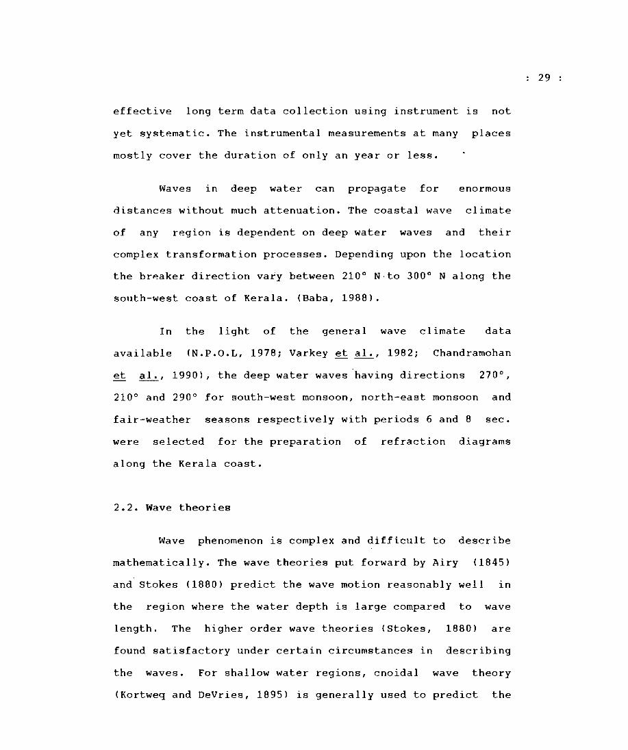
2.2. Wave theories

Wave phenomenon is complex and difficult to describe

mathematically. The wave theories put forward by Airy (1845)

and Stokes (1880) predict the wave motion reasonably well in

the region where the water depth is large compared to wave

length. The higher order wave theories (Stokes, 1880) are

found satisfactory under certain circumstances in describing

the waves. For shallow water regions, cnoidal wave theory

(Kortweq and DeVries, 1895) is generally used to predict the

29

30

form and associated motion. At very shallow regions, the

solitary wave theory (Russel, 1845; Boussinesq, 1872;

Rayleigh, 1876; McCowan, 1891; Keulegan, 1948; Iwasa, 1955)

can be used to describe the wave behaviour satisfactorily.

The regions of validity of various wave theories are

indicated by Le Mehaute (1969).

In shallow water region, particularly close to

breaking zone, the use of higher order wave theories would

provide more accuracy in the analysis. The appropriate wave

theories for the different regions are classified according

to the relative water depth as follows.

h/L Wave theory

> 0.2 stoke's III order

0.2 > = h/L> 0.05 Cnoidal

0.05 > = h/L > hb/L Solitary

where h is the water depth and L is the wave length.

2.2.1. Small amplitude wave theory

The elementary progressive wave theory referred to as

the small amplitud~ wave theory was developed by Airy (1845).

It is of fundamental importance because it is easy to apply

and reliable over a large segment of the whole wave regime.

While the exact wave theories are presented in series of

terms., the one with only the first term is called the small

amplitude wave theory. It assumes that the wave height (H) is

so small that all higher order terms can be neglected. In

31

this way, the free surface boundary condition is linearised

and the resulting approximate equatioh is obtained. The small

amplitude wave theory with the associated boundary conditions

give the phase velocity (Svendsen and Jonsson, 1976),

c = gT tanh kh ( 2 . 1 )

2 rI

u = (agk) :cosh k(h + z ) sin(kx-~t) ( 2 • 2 ) ----- -------------

0 cosh kh where

k = 2 IIIL

c = wave celerity

u = Horizontal particle velocity

a = wave amplitude

~= wave frequency = 2 rI I T

2.2.2. Finite amplitude wave theory

Once the wave amplitude become larger compared to wave

length the assumption of small amplitude wave theory is no

longer valid and it is necessary to retain higher order terms

to obtain an accurate representation of the wave motion. The

finite amplitude wave theory takes into account the

additional parameters H/h and H/L (where H is the w~ve

height), but it rapidly grows complicated with increasing

order of approximation.

2.2.3. Stoke's higher order wave theory

stoke's (1880) presented the approach and subsequently

many researchers extended the theory to various higher

orders. Using the third order equations, Miche (1944) has

given the following relationship for wave celerity.

C = gT I 2tl tanh kh (l+(rt H/L)2K,) ( 2 • 3 )

where K' = (S + 2 cosh 2kh + 2 cosh2 2kh)/(S sinh4 kh)

2.2.4. Cnoidal wave theory

The existence of long finite amplitude waves of

permanent form propagating in shallow water was first

recognised by Boussinesq (1872) and the theory was developed

by Korteweg and deVries (189S). The approximate range of

validity of cnoidal wave theory is 0.2 > h I L > O.OS or the

Ursell parameter (U=HL 2/h 3 »2S (Isobe, 1985). Wiegel (1960)

and Masch (1961) presented the wave characteristics in

tabular and graphical form to facilitate the application.

Svendsen (1974) presented the description of cnoidal

waves solving the Korteweg and deVries (Kdv) equation. The

solution of this equation is expressed by a Jacobian elliptic

function c n of two variables, ~ and a parameter m (~ <=m <1)

n min+ H 2 (IP,m) ( 2 • 4 ) lJ = c n

'lmin = (l/m)«l-E/K)-l)H ( 2 • S )

where

IJmin = distance of trough from the mean water level

K = K (m) , complete elliptic integrals of the first kind

E = E (m) , complete elliptic integrals of the second

kind

32

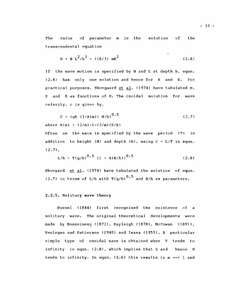
The value of parameter m is the solution of the

transcendental equation

( 2 .6)

If the wave motion is specified by Hand L at depth h, equn.

(2.6) has only one solution and hence for K and E. For

practical purposes, Skovgaard et al. (1974) have tabulated m,

K and E as functions of U. The cnoidal solution for wave

celerity, c is given by,

C = (gh (l+A(m» H/h)0.5

where A(m) = (2/m)-1-(3/m)(E/K)

( 2 .7)

Often as the wave is specified by the wave period (T) in

addition to height (H) and depth (h), using C = LIT in equn.

( 2 ~ 7 ) ,

L/h

Skovgard

= T(g/h)0.5 (1 + A(H/h»O.5

et al. (1974) have tabulated the solution -- --

( 2 . 8 )

of equn.

(2.7) in terms of L/h with T(g/h)0.5 and H/h as parameters.

2.2.5. Solitary wave theory

Russel (1844) first recognised the existence of a

solitary wave. The original theoretical developments were

made by Boussinesq (1872), Rayleigh (1878), McCowan (1891),

Keulegan and Patterson (1940) and Iwasa (1955). A particular

simple type of cnoidal wave is obtained when T tends to

infinity in equn. (2.8), which implies that Land hence U

tends to infinity. In equn. (2.6) this results in m --) 1 and

33

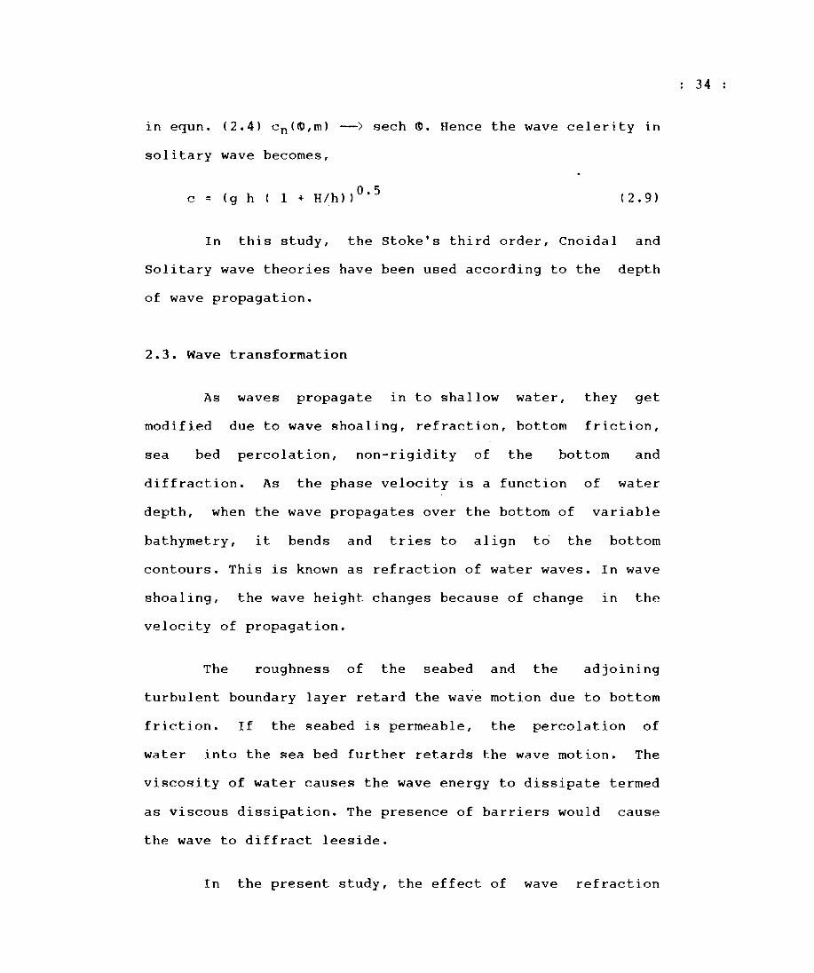
in equn. (2.4) cn(~,m) --> sech ~. Hence the wave celerity in

solitary wave becomes,

c = (g h ( 1 + H/h»O.5 ( 2 . 9 )

In this study, the stoke's third order, Cnoidal and

Solitary wave theories have been used according to the depth

of wave propagation.

2.3. Wave transformation

As waves propagate in to shallow water, they get

modified due to wave shoaling, refraction, bottom friction,

sea bed percolation, non-rigidity of the bottom and

diffraction. As the phase velocity is a function of water

depth, when the wave propagates over the bottom of variable

bathymetry, it bends and tries to align to the bottom

contours. This is known as refraction of water waves. In wave

shoaling, the wave height changes because of change in the

velocity of propagation.

The roughness of the seabed and the adjoining

turbulent boundary layer retard the wa~e motion due to bottom

friction. If the seabed is permeable, the percolation of

water into the sea bed further retards the wave motion. The

viscosity of water causes the wave energy to dissipate termed

as viscous dissipation. The presence of barriers would cause

the wave to diffract leeside.

In the present study, the effect of wave refraction

34

and wave shoaling are considered. Assumption made in

estimating the nearshore wave transformation are,

(1) The wave energy transmitted between adjacent wave

orthogonals remain constant. The lateral dispersion of

wave energy along the wave front, reflection of energy

from the sloping bottom and the loss of energy by other

processes are negligible.

(2) Waves are long crested and of constant period.

(3) Curvature of the wave front is small so that it has

negligible effect on the velocity of propagation.

(4) Effect of wind, current and reflection from beaches are

negligible.

(5) Changes in bottom topography is gradual."

(6) No crest breaking during propagation.

2.3.1. Shoaling

The wave power transmitted forward between two orthogonals in

deep water

( 2 . 10 )

where bo is the distance between the selected orthogonals in

deep water, Eo is the energy transmitted between two

orthogonals in deep water and Co is the phase velocity in

deep water.

The power equated to the energy transmitted forward between

the same two orthogonals in shallow water

P=n b E (2.11)

35

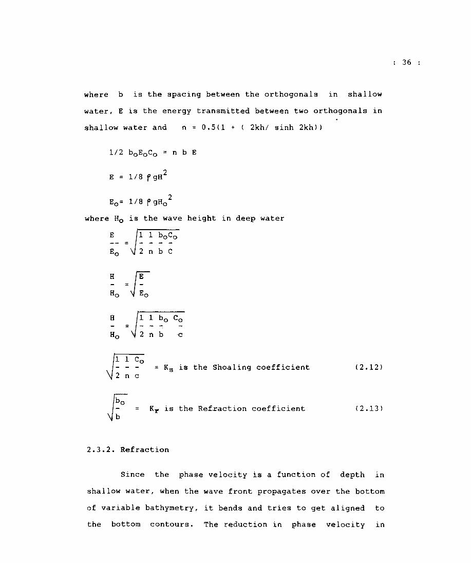
where b is the spacing between the orthogonals in shallow

water, E is the energy transmitted between two orthogonals in

shallow water and

E = 1/8fgH2

2 Eo= 1/8 t' gHo

n = 0.5(1 + ( 2khl sinh 2kh»

where Ho is the wave height in deep water

= - - - -Eo 2 n b C

H =f[ H

= - - -2 n b ·c

l- 1_ C_o = Ks is the Shoaling coefficient 2 n c

[_0 __ Kr is the Refxaction coefficient

b

2.3.2. Refraction

(2.12)

(2.13)

Since the phase velocity is a function of depth in

shallow water, when the wave front propagates over the bottom

of variable bathymetry, it bends and tries to get aligned to

the bottom contours. The reduction in phase velocity in

36

shallow water causes refraction in a process analogous to

Snell's law in geometrical optics. Then the change in

direction of orthogonal as it passes over relativ~ly simple

bathymetry may be approximated by,

s in QC 2 = C2 /C l since 1

0<:1 = angle of wave crest make with the bottom contour

OC2 = angle of wave crest for the next bottom contour

Cl = wave velocity at a depth of first contour

C2 = wave velocity for the next contour.

The spacing between orthogonals indicate the amount of

concentration or dispersion of energy. Wave rays are normal

to the crests and are therefore in the direction of wave

advance and energy propagation. The wave power is conserved

between adjacent rays, so that a convergence of rays implies

a focusing of the ·wave energy leading to greater wave heights

and progressive separation of rays represents defocussing.

For straight and parallel contours, the orthogonals would be

parallel and the horizontal distance is constant between two

adjacent orthogonals. Therefore,

bol cos cc 0 = bl coscx:

bo/b = cosocol coso:

Kr = (bo/b)O.S = (cosoc o Icoscx:)O.S ( 2 • 5 )

where CC is the angle between two orthogonals ln shallow water

andOCois the angle between two orthogonals in deep water.

For a given topography and deep water wave

characteristics, the refracted orthogonals can be plotted by

37

geometrical procedure (Anonymous, 1975). The graphical method

of wave refraction analysis by Arthur et al. (1952), has been

widely used till recently for computation of wave refraction.

Studies using graphical method are many for the Kerala coast

as well as other part of the country, which have been

reviewed earlier (Chapter I). Many refinements have been made

relating to the direct construction of refraction diagrams

based on the wave crest method (Johnson, 1947) and orthogonal

method. Recently computer based numerical methods for

determining refraction characteristics have been used

(Griswold, 1963; Harrison and Wilson, 1964; Wilson, 1966;

Dobson, 1967). While these computer methods are undergoing

considerable refinement, they are operational and may result

in significant time saving in refraction computations over a

relatively large area.

Refraction studies based on the numerical models are

scanty for the Kerala coast. A study of the wave

transformation using a numerical model along the Kerala coast

by making synchronized measurements of deep and shallow water

waves has been done by Kurian (1987). For a given bathymetry

and deep water characteristics, numerical wave transformation

models incorporating shoaling and refraction have been

developed by many researchers. (Skovgaard et ~., 1975;

Griswold, 1963; Harrison and Wilson , 1964; Orr and Herbich,

1969; Jen, 1969). Most of the numerical refraction model have

used the linear wave theory and a few have attempted using

finite amplitude wave theories.

38

2.3.3. Numerical wave refraction

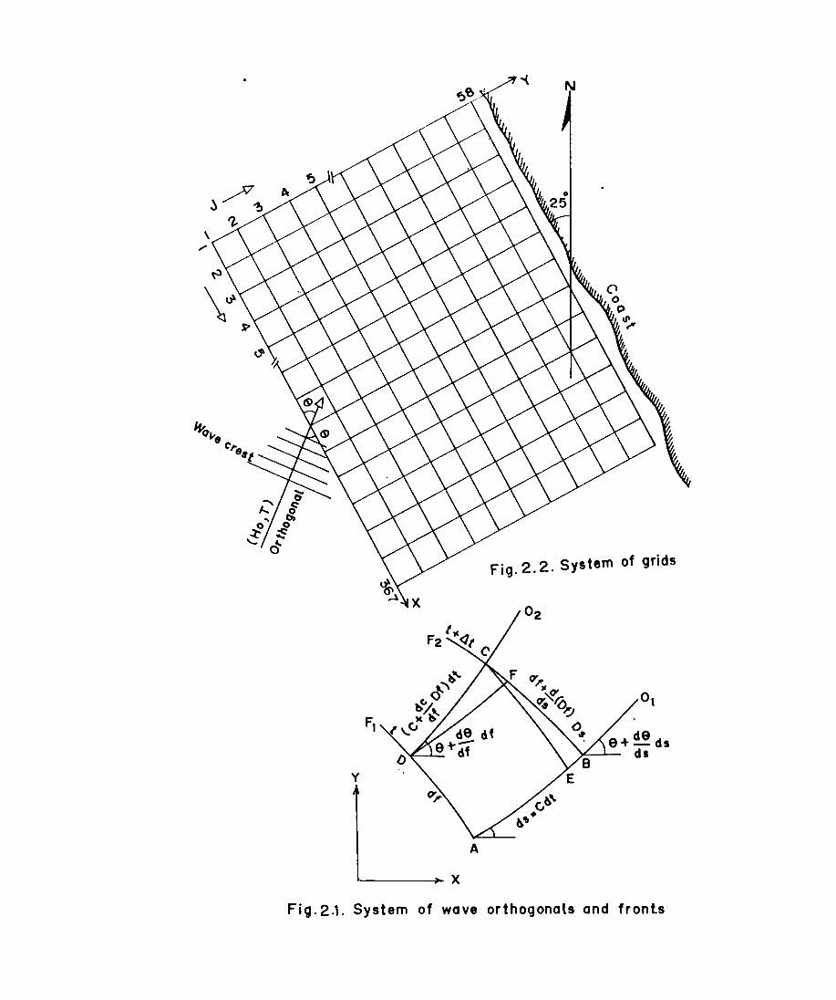
Fig. 2.1 shows the adjacent orthogonals 01, 02 and

two consecutive wave fronts F1, F2 separated by time interval

dt (Skovgaard et al., 1975). At point A, the infinitesimal

distance between orthogonals and fronts are Of and Os

respectiv~ly, where,

Os = c dt (2.16)

The distance s is taken as positive in the direction of wave

propagation and the positive direction of f is such that Os

and Of form a right hand coordinate system. m is the angle

between the x axis and the orthogonal, positive in

anticlockwise direction.

From the triangles BCE and COF,

Curvature of wave ~rthogonal = O~/Os = -(l/c) (Oc/Of) (2.17)

Curvature of wave front = Om/Of = (1/0f) (O(Of)/Os) (2.18)

Defining the following operators as

O/Os = cos (0 (d/dx) + sin <D (d/dy)

O/Of = sin (0 (d/dx) + cos <D (d/dy)

and using equns. (2.16 ) and (2.17),

(2.19)

( 2 • 20 )

dtO/dt = - (Oc/Of) (2.21>

Using equns. (2.17), (2.18), (2.19), (2.20) and (2.21), the

basic equations for the wave orthogonals become,

dx/dt = c cos to

dy/dt = c sin (0

dtO/dt = (dc/dx) sin (0 - (dc/dy) cos 0

(2.22)

( 2.23)

(2.24)

39

\ ,.

N

Fig. 2.2. System of grids

y

A

'-----~ X

Fig.2.1. System of wave orthogonals and fronts

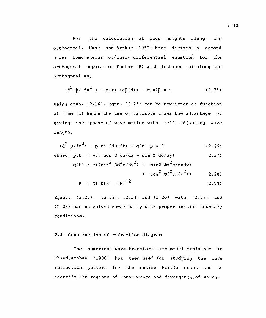
For the calculation of wave heights along the

orthogonal, Munk and Arthur (1952) have derived a second .

order homogeneous ordinary differential equation for the

orthogonal separation factor (~) with distance(s) along the

orthogonal as,

( 2 • 25 )

Using equn. (2.1~), equn. (2.25) can be rewritten as function

of time (t) hence the use of variable t has the advantage of

giving the phase of wave motion with self adjusting wave

length,

(d2 J3/dt 2 )

where, p(t) =

q(t) =

f3 =

+ p(t) (dJ3/dt) + q(t) P = 0

-2( cos <D dc/dx - sin <D dc/dy)

c ( ( sin 2 <Dd 2c/dx 2 ) (-sin2 2 - <Dd c/dxdy)

+ (cos 2 <Dd 2c/dy2))

Df/Dfst -2 = Kr

(2.26)

(2.27)

( 2 • 28 )

(2.29)

Equns. (2.22), (2.23), (2.24) and (2.26) with (2.27) and

(2.28) can be solved numerically with proper initial boundary

conditions.

2.4. Construction of refraction diagram

The numerical wave transformation model explained 1n

Chandramohan (1988) has been used for studying the wave

refraction pattern for the entire Kerala coast and to

identify the regions of convergence and divergence.of waves.

40

Referring to the section 2.2, based on the wave

climate of Kerala coast the three predominant wave o

directions, 270 for south-west monsoon period (June-

September), 210 0 for north-east monsoon period (October-

January) and 290 0 for fair-weather period (February-May) were

selected for the construction of wave refraction diagrams.

Reflection and diffraction were not considered for this coast

whiC!h is straight and open.

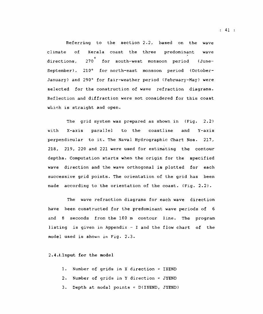
The grid system was prepared as shown in (Fig. 2.2)

with X-axis parallel to' the coastline and Y-axis

perpendicular to it. The Naval Hydrographic Chart Nos. 217,

218, 219, 220 and 221 were used for estimating the contour

depths. Computation starts when the origin for the specified

wave direction and the wave orthogonal is plotted for each

successive grid points. The orientation of the grid has been

made according to the orientation of the coast. (Fig. 2.2).

The wave refraction diagrams for each wave direction

have been constructed for the predominant wave periods of 6

and 8 seconds from the 100 m contour line. The program

listing is given in Appendix - I and the flow chart of the

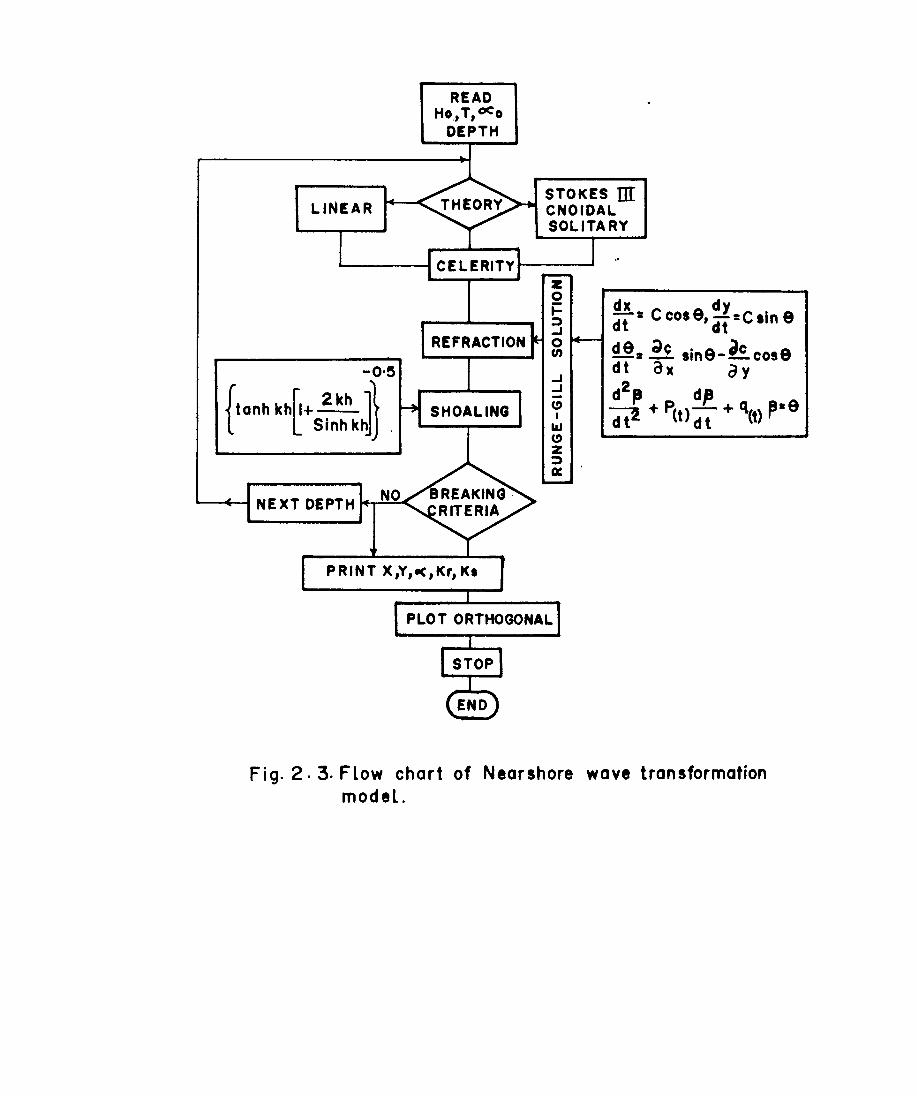
model used is shown in Fig. 2.3.

2.4.I.Input for the model

1. Number of grids in X direction = IXEND

2. Number of grids in Y direction = JYEND

3. Depth at nodal points = D(IXEND, JYEND)

41

LINEAR

-O'~

{ tanh khrl+ 2 kh J~ L Sinh khlJ .

~+-I NEXT DEPTH ~~~

READ Ho" T,ceo

DEPTH

STOKES m CNOIDAL SOLITARY

...I

...I (!) I

I&J (!) Z :;)

a:

Fig. 2. 3. Flow chart of Nearshore wave transformation model.

4.

5.

6.

7.

8.

Distance between the grids (metres)

Slope of the sea bed = SLOPE

Starting point of wave orthogonal in

Starting point of wave orthogonal in

Deep water wave height (m) = H

9. Wave period (s) = T

= SCA

X direction

Y direction

10. Direction of wave crest with X axis (deg) = THETA

(wave crest to X axis anticlockwise positive)

11. Wave theory = LINEAR/HIGHER

12. Time step = T

13. stop computation at - BREAKING/GIVEN DEPTH

computation stops at one of the following condition:

1. Wave steepness

2. breaking depth

H/L = 0.172 tanh kh

db = 1.28 Hb

=

=

3. orthogonal reaches the sides/shore/required depth.

X

y

Output Output of the model consists of grid locations of the

orthogonals at different time, deformed wave crest

direction, shoaling and refraction coefficients and

the net wave breaker heights.

2.5. Results

The numerical wave refraction study was undertaken to

find out the distribution of wave energy along the Kerala

coast. The refraction diagrams for different incoming wave

directions and different wave periods are presented 1n

(Figs. 2.4a & 2.4b), (Figs. 2.5a & 2.5b) and (Figs. 2.6a &

42

2.6b). The pattern of wave refraction according to the

different seasons are described below.

South-west monsoon period (Wave direction 2700 , Wave period

: 6 Sand 8 S)

The refraction diagram for the predominant wave

periods 6 Sand 8 S for the wave direction 2700 with respect

to north are presented in (Fig. 2.4a) and Fig. (2.4b)

respectively.

(Fig. 2.4a) shows convergence of wave orthogonals only

at Vypin, north of Cochin. The divergence of wave orthogonals

is observed south of Ezhimala, south of Cannanore, at

Quilandi, Quilon, Varkallai and Puvar. The remaining stretch

of the coast experiences nearly uniform wave energy for this

direction of wave approach and wave period.

Waves approaching from 2700 with respect to north and

with 8 S period, show more convergence of energy along the

coast than waves of 6 S period (Fig. 2.4b). Convergence of

wave energy is observed at Kasargod, south of Cannanore,

North of Quilandi, south of Beypore, at Ponnani, Vypin, north

of Alleppey, north of Karunagappalli and at Neendakara. The

divergence of wave orthogonals is seen south of Ezhimala,

Andhakaranazhi and Quilon. Along the rest of the coastal I

stretch, it is seen that the wave energy is uniformly

distributed.

43

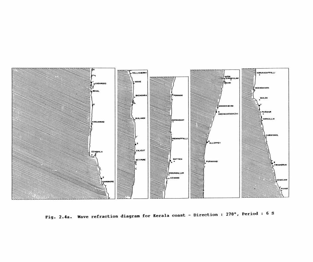
Fig. 2.4a. Wave refraction diagram for Kerala coast - Direction 210°, Period 6 S

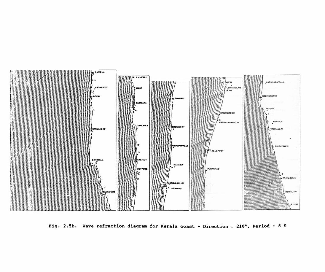
North-east monsoon period (Wave direction 2100 , Wave

period : 6 Sand 8 S)

The wave orthogonals approaching the coast· at 210 0

with respect to north for the wave periods 6 S and 8 S are

presented in (Fig. 2.5a) and (Fig. 2.5b) respectively.

The refraction diagram for the wave period of 6 S

(Fig. 2.5a), shows convergence of wave energy north of

Kanjangad, at Vypin and at Purakkad. The divergence of wave

orthogonals is seen along the coast south of Ezhimala,

between Cannanore and Mahe, Quilandi and further south and

Quilon. It is seen that remaining stretch of the coast is

subjected to uniform distribution of wave energy.

(Fig. 2.5b), for the 8 S waves shows, convergence of

wave energy along south of Kasargod, Kanjangad, north of

Ponnani, Azhikod, Vypin, north of Alleppey, Purakkad and

Neendakara and divergence of wave orthogonals near Cannanore

upto Badagara, Mahe, south of Nattika, Andhakaranazhi and

north of Karunagappalli. The wave energy is uniformly

distributed along the other parts of the stretch of this

coast.

Fair-weather season (Wave direction

and 8 S)

290°, Wave period 6 S

The refraction of wave orthogonals for the direction

2900 with respect to north for wave periods 6 Sand 8 S are

presented in (Fig. 2.6a) and (Fig. 2.6b).

44

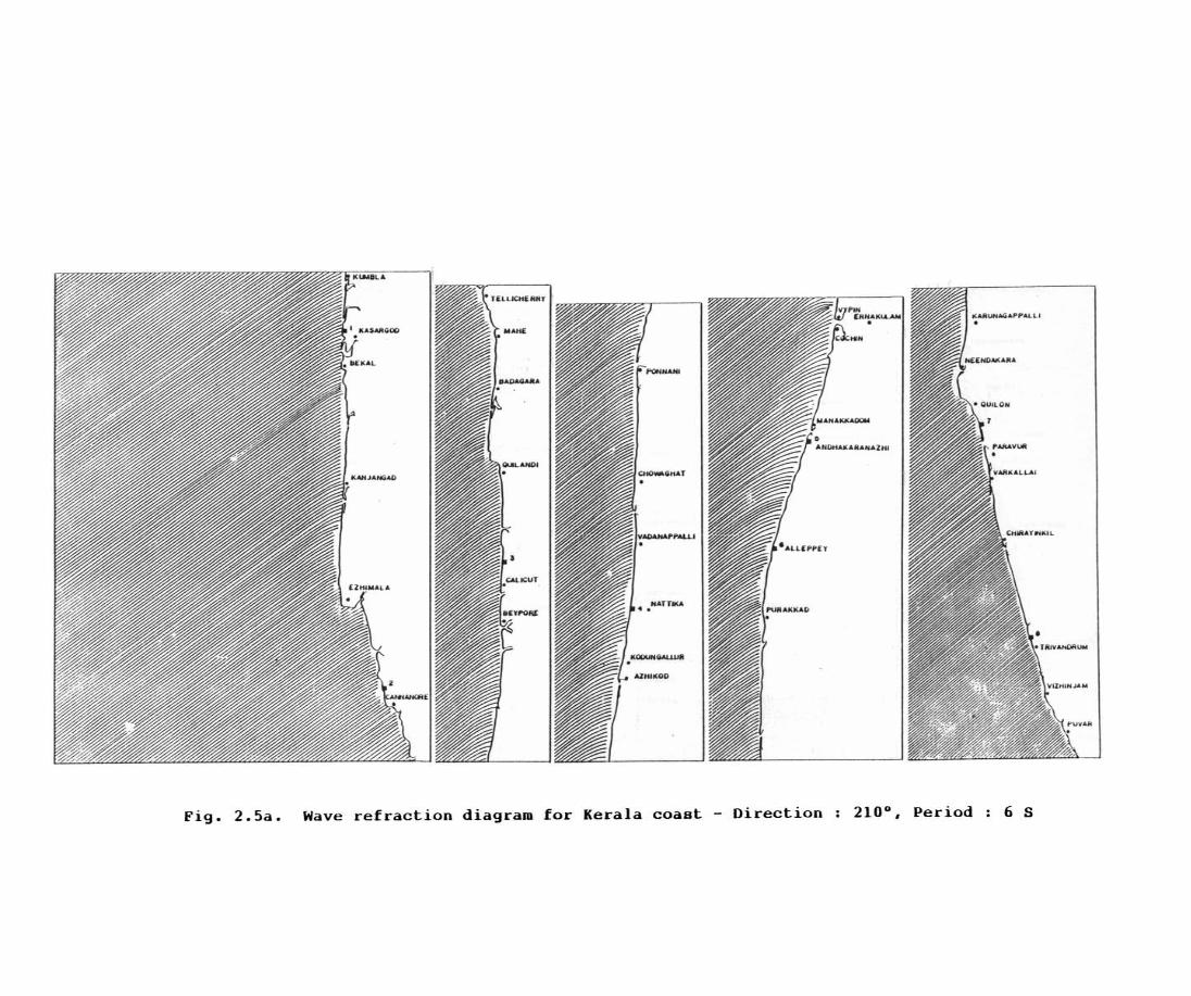
Fig. 2.5a. Wave refraction diagram for Kerala coast Direction 210°. Period 6 s

PUVAR

Fig. 2.5b. Wave refraction diagram for Kerala coast Direction 210°, Period 8 S

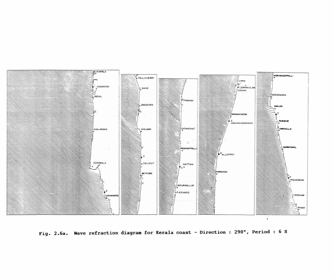
Fig. 2.6a. Wave refraction diagram for Kerala coast - Direction 290°, Period 6 S

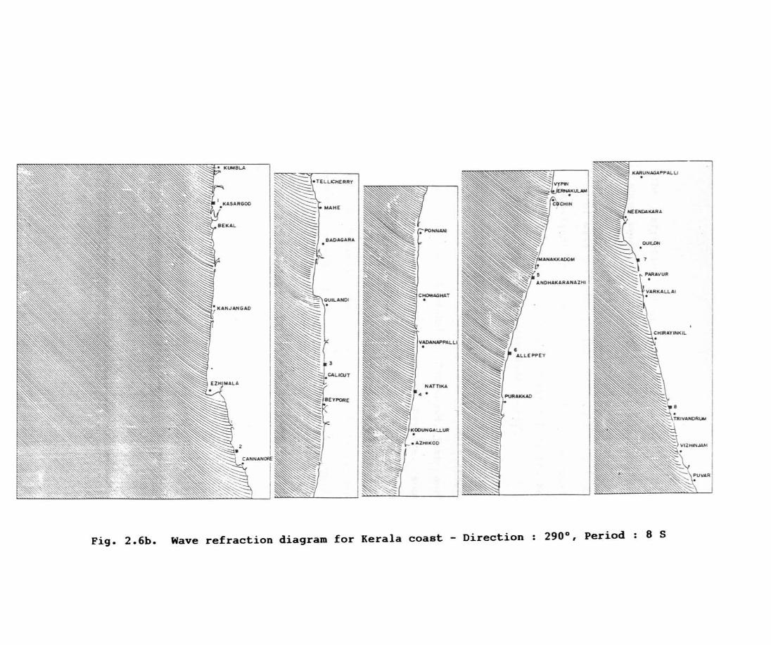
Fig. 2.6b. Wave refraction diagram for Kerala coast - Direction 290°, Period 8 S

2. 6a) ,

Bekal,

The refraction diagram for wave period 6 S (Fig.

shows convergence of wave orthogonals along north

south of Ponnani, at Vypin and Purakkad.

of

The

divergence of wave orthogonals are observed from Ezhimala to

Mahe, at Quilandi, Nattika, Andhakaranazhi, from Quilon to

Varkallai and at Puvar. The remaining stretch of the beach is

subjected to more or less uniform wave energy.

(Fig. 2.6b), for the 8 S period shows that the waves

approaching the coast with a direction 2900 with respect to

north converge at south of Bekal, Kanjangad, just north of

Cannanore, south of Quilandi, south of Beypore, south of

Ponnani, Azhikod, Vypin, north of Alleppey, north of Purakkad

and at Neendakara. Divergence of the. wave energy is observed

at North of Ezhimala, Cannanore to Tellichery, Nattika,

Andhakaranazhi north of Karunagappalli, along Quilon to

Varkallai and at Puvar. The remaining part of the coast

experiences direct attack of waves without appreciable

refraction.

·2.5.1. Variation of breaker parameters

Based on the numerical wave refraction study, the

shoaling coefficient (Ks), refraction coefficient (Kr) just

before wave breaking, and the variation of breaker height

(Hb) for the entire Kerala coast were estimated and presented

in (Figs. 2.7a & 2.7b), (Figs. 2.8a & 2.8B) and (Figs. 2.9a &

2. 9b) •

45

South-west monsoon period (Wave direction

: 6 Sand 8 S)

270°, Wave period

The shoaling coefficient (Ks) for 6 S waves

approaching from 270°, (Fig. 2.7a), shows relatively large

values ()0.95) at Ezhimala, Cannanore, Quilandi, Cochin and

between Quilon and Trivandrum. Ks shows values around 0.9 at

all the other places.

For 8 S waves approaching from 270° (Fig. 2.7b), the

value of the shoaling coefficients (Ks) is less than 1 at

most of the places. But in some places it shows values

greater than 1 (Ezhimala, Cannanore, Mahe, Quilandi, Nattika,

Vypin and at South of Alleppey).

The value of the refraction coefficient (Kr) is very

important because the wave energy distribution

beach depends on Kr. From (Fig. 2.7a) it is clear

along

that

the

for

waves approaching the coast from this predominant directions

of 2700 with period 6 S, the Kr values at the breaking point

are greater than 1 north of Ezhimala, at Vypin,

Andhakaranazhi, Alleppey and north of Quilon. The Kr value is

very low along south of Ezhimala and along south of Quilon.

The refraction coefficient (Kr) presented in (Fig.

2.7b), for 8 S period waves, shows values greater than 1

north and south of Ezhimala, Kanjangad, south of Beypore,

south of Bekal, between Vypin and south of Alleppey and

Quilon. Kr values are low around 0.6 north of Quilon and at

Varkallai. The lowest value of 0.5 is observed near Puvar.

46

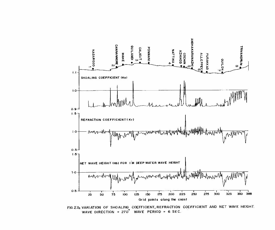
n 0 ,.

n "V

" z c ,. 0 z ,. z r r z !i

,. (I)

,. ~ ,.

(') Z NO ,. z ,. z c ,. -t %0 :u ~ % 2 ~-t z -0 Gl '" ~ ~%

N~ ~,. 0_

0 • Oz ...... 0 • •

I --.! I.Il

SHOALlNG COEFFICIENT CKs)

1·0 I I IIA

0.9

I.~

REFRACTION COEFFICIENT C Kr)

J> Z 0 % ,. ~ ,. :u ,. z ,. N %

1·0 I fi.;M1l ;>1~Ajvvd • I lA It • iliA ./LJ;rcJ.A - h_A i i ,11,111111. III ,dUlRLlIII/IRlI . I i - A. IN . (- •• AA

0.5

I.~

NET WAVE HEIGHT CHb) FOR I M DEEP WATER WAVE HEIGHT

1· 0 I i I all i Ad.- Al

O.~~----~----r----'~--~-----r-----.----'-----~----r---~r----'~---.-----r-----r----'

25 50 75 100 125 1:50 17~ 200 225 2:50 275 300 325 350 368

Grid points along the coast

FIG.2J'o. VARIATION OF SHOALlNG COEFFICIENT. REFRACTION COEFFICIENT AND NET WAVE HEIGHT. o

WAVE DIRECTION = 270 WAVE PERIOD = 6 SEC.

(')

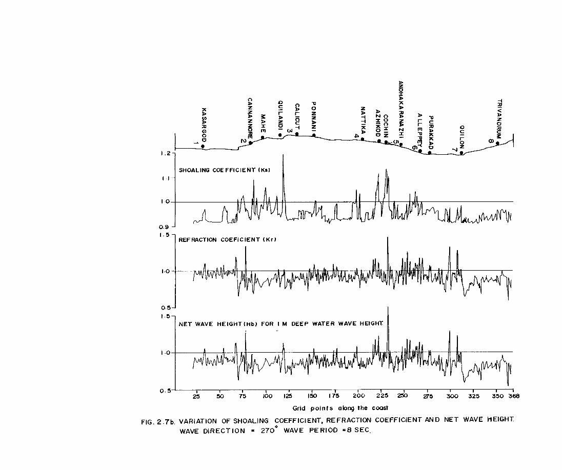
> z " z > > ~ (I) z > ~

Z 7 ::u 0 111 Cl ~ 0

0 I\> •

1.2

SHOALlNG COEFFICIENT (Ks)

1·1

0 -u c (') 0 > r r z

> n z z c ~ !2 V'-t Z

•

z ~ -t -t

" ~~

J> Z o 7 ~

" > ~ ~

I 0 I l fI Jll I \ A ~ 1\ n ~ I I',{ I A . J ~/h . 1 \ .1 n I

0.9 1.5

REFRACTION COEFICIENT (Kr)

1·0 I 1Vii\/IIAI\A~~Arl,1\ .11 ..1 J . .ft.AA lb. ~~ 11 d I APIIIA.1I11 t\ljl~UMVH\ M AI 11 I~n

0.5

1·5 NET WAVE HEIGHT (Hb) FOR I tot DEEP WATER WAVE HEIGHT.

1·0 I A 1\ I 11

~

0.5 I I I' I I I , I I .,' 25 50 75 100 125 150 175 200 225 250 215 300 325 350 368

Grid points olong the coast

FIG. 2.7b. VARIATION OF SHOALlNG COEFFICIENT, REFRACTION COEFFICIENT AND NET WAVE HEIGHT o

WAVE DIRECT ION = 270 WAVE PE RIOD "8 SEC

The breaking wave heights (Hb) along the Kerala

coast, evaluated from Ks and Kr for unit deep water height

for 6 S waves are presented in (Fig. 2.7a). Increase in net

wave height ( >1 m) is observed at Quilandi, Vypin, North of

Alleppey and Quilon. The highest breaker height of 1.5 m is

observed near Vypin. Breaker height is around 0.8 m along the

remaining stretch of the Kerala coast. Low breaker height is

observed at Calicut beach.

The breaker height distribution (Hb) for 8 S period

waves (Fig. 2.7b) shows that the breaker heights are more

than the deep water wave height at Kasargod, Kanjangad, north

of Ezhimala, south of Rekal, Quilandi, south of Beypore,

Ponnani, Nattika, Vypin, Andhakaran~zhi, Alleppey and Quilon.

Along the rest of the coast, the. breaker heights are less

than (0.6 m - 0.9 m times) the deep water wave height. Lowest

breaker height is observed near Puvar.

North-east monsoon season (Wave direction

: 6 Sand 8 S)

210°, Wave period

(Fig. 2.8a), shows that for waves approaching from

210 0 with respect to north with period 6 S, the shoaling

coefficient (Ks) is greater than 1 at Quilandi, north of

Nattika, Vypin and at Alleppey. At all the other places it is

around 0.95.

waves

The shoaling

(Fig. 2.8b),

coefficient values (Ks), for the 8 S

are greater than unity at Cannanore,

47

0 J> 0 ""0 z c 0 0 ~ z r J> z z J> J> r J>

(/) J> ~ J> (; Z , NO J> Z J> Z J> , :1:0 :u z :r 2 VI ~ z -0

Cl 0 '" ~ 6!

0 :u • ~J> Oz N'" ~o r(JI •

1.2 1 -1 SHOALlNG COEFFICIENT IK.I

1.1

1·0 I 11 III I

0.9

1.5

REFRACTION COEFFICIENT (Kr)

1> Z 0 :r J> ~ J> :u J> J> ""0 Z r C J> r :u N '" J> 0 :r ... c

1·0 l A A • L. . loAlI fIlA. 11 ~"J\, ::;>

0.5 1.5

.. NET WAVE HEIGHTCHb) FOR I M DEEP WATER WAVE HEIGHT

I ·0 I 1\ l

, :u <: J> Z 0 :u C ~

0.5~----.-----.-----r----.-----.-----.----~----~----r---~~--~----~----~----~~

25 50 75 100 125 150 175 200 225 250 275 300

Grid points alon9 the coast

325 350 368

FIG.2.8a. VARIATION OF SHOALlNG COEFFICIENT, REFRACTION COEFFICIENT AND NET WAVE HEIGHT. o

WAVE DIRECTION'" 210 WAVE PERIOD'" 6 SEC.

~ 0 :r

" l> ~ "

(/) Z

C 0 -0

l> l> ~

r= l> 0

:u Z l>

l> r Z

Cl Z :r

Z (") Z

0 i 0 C l>

0

1'1\ (H-i Z

• • -

l>

" l> ~ l>

~ Ii' -0 NO r C

" -i :ro

~ r ;u c

::! -0 1'1\ l> " l§~ N ~ " r

l> Oz ~

" 0 ~-

l> -..I Z 0

1.3

1.2-1 SHOALlNG COEFFICIENT (Ks)

1.1

1.0 I kA AlII I ."A }I l 11 ,9" N I I 1 I ill h IY

0.9 1.5

REFRACT ION COE FF I C lE NT (Kr)

1·0 I. . I • Ill. ~ AI. I I 11 Hili A U

0.5 1.4

0.9

NET WAVE HEIGHTtHb) FOR I M DEEP WATER WAVE HEIGHT

0·4 I I I I I I I 25 50 75 100 125 150 175 200 225 250 275 300 325 350 368

Grid pOints along the coast

FIG. 2.8 b.VARIATION OF SHOALlNG COEFFICIENT. REFRACTION COEFFICIENT AND NET WAVE HEIGHT

WAVE DIRECTION ~ 210 0 WAVE PER 100 ~ 8 SEC.

Quilandi, Ponnani, north of Nattika, Vypin, north of

Alleppey, and north of Quilon. Along the remaining stretch of

the coast, the values are around 0.95.

The refraction coefficient (Kr) for 6 S period waves

shows values greater than 1 at Kasargod, Ezhimala,

Cannanore, Quilandi, Vypin, south of Alleppey and Quilcn. All

the other places, it ranges between 0.5 to 0.9.

The refraction coefficient (Kr) estimated for 8 S

period waves shows that the values are greater

Ezhimala, Cannanore, south of Chawaghat, North

Vypin, north of Alleppey, Purakkad and Quilon.

than 1 at

of Nattika,

The breaker height parameter (Hb) computed for the

waves approaching from 210° with 6 S period, indicates high

values at Vypin and Quilon. Between Andhakaranazhi and

Alleppey, the values show a minimum breaker height for this

period and direction (0.6m). At other places, it is 0.75 of

the deep water wave height. The highest breaker height of 1.4

m is observed north of Cochin.

For the direction of approach of 210°, waves with

period 8 S show net breaker height (Hb) greater than 1 at

Ezhimala, Cannanore, Vypin, north of Alleppey, Purakkad and

north of Quilon. At Vypin, the wave breaker heights get

amplified and show values around 1.3m for the deep water wave

of 1m. At places between Nattika and Andhakaranazhi, Hb shows

values around 0.5m while at Kasargod it is 0.9 m.

48

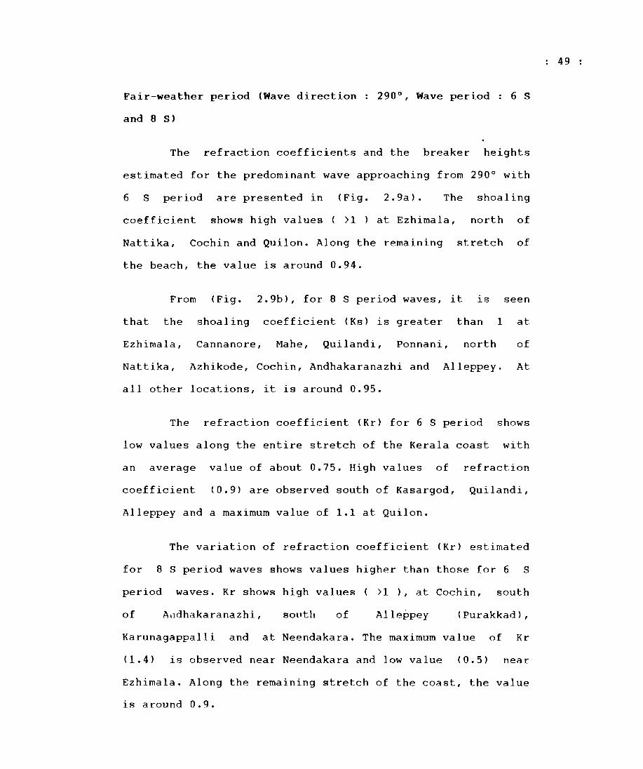
Fair-weather period (Wave direction

and 8 S)

290°, Wave period 6 S

The refraction coefficients and the breaker heights

estimated for the predominant wave approaching from 290 0 with

6 S period are presented in (Fig. 2.9a). The shoaling

coefficient shows high values ( >1 ) at Ezhimala, north of

Nattika, Cochin and Quilon. Along the remaining stretch of

the beach, the value is around 0.94.

From (Fig. 2.9b), for 8 S period waves, it is seen

that the shoaling coefficient (Rs) is greater than 1 at

Ezhimala, Cannanore, Mahe, Quilandi, Ponnani, north of

Nattika, Azhikode, Cochin, Andhakaranazhi and Alleppey. At

all other locations, it is around 0.95.

The refraction coefficient (Rr) for 6 S period shows

low values along the entire stretch of the Kerala coast with

an average value of about 0.75. High values of refraction

coefficient (0.9) are observed south of Rasargod, Quilandi,

Alleppey and a maximum value of 1.1 at Quilon.

The variation of refraction coefficient (Kr) estimated

for 8 S period waves shows values higher than those for 6 S

period waves. Rr shows high values >1), at Cochin, south

of A~dhakaranazhi, soptll of Alle~pey (Purakkad),

Karunagappalli and at Neendakara. The maximum value of Rr

(1.4) is observed near Neendakara and low value (0.5) near

Ezhimala. Along the remaining stretch of the coast, the value

is around 0.9.

49

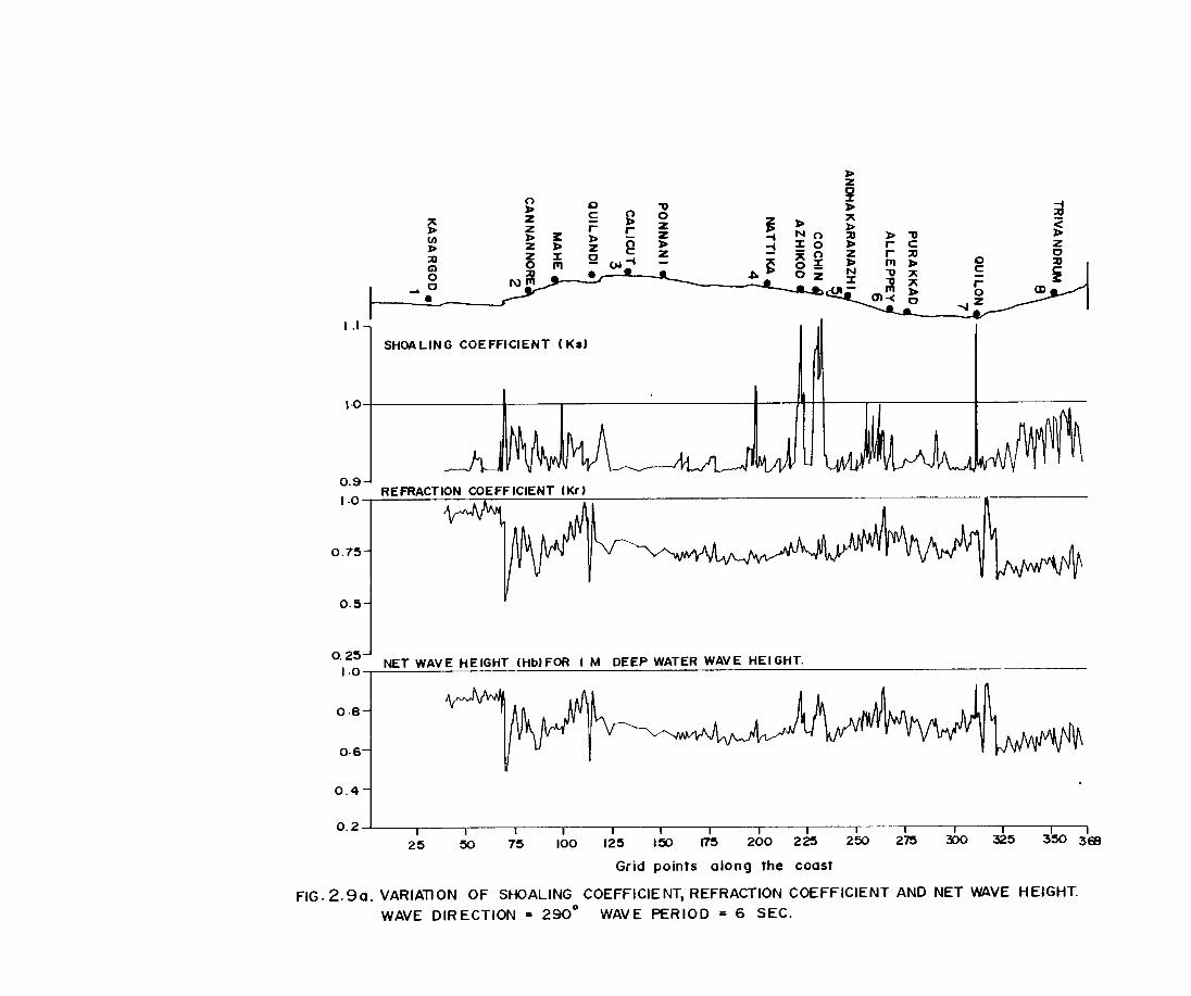
0 "V s: ~ 0

" ~ z :.:. ;z r- r !E J: loo -=

I .I

SHOALING COEFFICIENT (KsJ

loo Z §! loo

i :.:. ~ :.:.

-t NO :u :.:. z :.:. N ::r

(J)

iJ i z o :u i

J~ I I 1.0l,------------~~~--r---~--~----------1----J~t---lrr---------1-----------0.9

REFRACTION COEFFICIENT lKrJ 1·0 . i

0.75

0.5

O·I~~ NET WAVE HEIGHT (HbJFOR I M DEEP WATER WAVE HEIGHT.

0·8

0·6

0.4

I I 0.2 50 25 75 100 125 150 rT5 200 225 250 275 300 325 350 368

Grid points along the coast

FIG. 2.90. VARIATION OF St-K>ALlNG COEFFICIENT, REFRACTION COEFFICIENT AND NET WAVE HEIGHT. WAVE DIR ECTlON = 2900 WAV E PERIOD ~ 6 SEC.

~ :r > 0

\J ~

s; 0 0 z > ::u

4<- r > z !i NO > " Z > r z :LO Z

l> l> 3: z 0 -i -0

> i'I ::u 0 1>

"I C

en z 1> C C Z

" O_ N \J l>

l> Z I OJ-i -

~> C z I ~ " r

::u 0 111

UI-

" 0

Cl ::u • • --- 1>

...,jZ

0 N~

• C .......

1.2 SHOA LING COEFFICIENT (Ks)

1.1

1\ A I1 if bel l 1111 /lMI i. ! . J '·0 , '.IId . Nil'!. 1\ M. 'Vv~

0.9

1.4

n;-PJ,

0.9

0.4

1.5

1.2

09

0·6

REFRACTION COEFFICIENT (Kr)

NET WAVE HEIGHTCHb) FOR I M DEEP WA'rER WAVE HEJGHT

I 0.3 I I I I I I I I I I I I I

25 ~ 75 100 125 I~ 175 200 225 250 275 300 325 3~ 368

Grid points along the coast

FIG.2.9b. VARIATDN OF SHOALlNG COEFFICIENT. REFRACTION COEFFICIENT AND NET WAVE HEIGHT.

WAVE DIRECT ION ~ 2900 WAVE PERIOD· 8 SEC.

The breaker height estimated for the predominant wave

direction of 290 0 with period 6 S, shows that the wave height

ia getting reduced and the breaker height never exceeded the

deep water wave height of 1 m. It shows an average value of

about 0.8 m along the stretch of the Kerala coast with low

values at Ezhimala (0.5 m) and Quilandi (0.6 m). Low values

of about 0.7m have been observed between Calicut and Nattika

and shows a maximum value of 0.9 m at Quilon.

The breaker height distribution (Hb) for 8 S period

waves shows higher values for the stretch of the coast from

Cochin to Quilon. Hb is greater than 1m at Cochin, Alleppey,

Purakkad and Neendakara. It shows high values north of

Alleppey (1.4 times the deep water wave height) and at Quilon

(1.3 times). At the southern end of the Kerala coast, Hb iR

only 0.4 times the initial deep water wave height for this

wave direction and period.

50

CHAPTER 3

3. BEACH DYNAMICS

3.1. Beach morphology

Beach is the most dynamic zone of the coastal

environment which is subjected to a wide range of variations.

The changes in beach profile are caused, to a large extend,

by the variations in the incident wave energy and fluctuation

in the position of the mean water level induced by tidal

oscillations. Seasonal changes of the beaches constitute an

important aspect of the coastal environment and hence data on

beach profiles along with constituent sediment provide vital

information on the energy levels to which this environment is

subjected to. Though our understanding of such changes

improved qualitatively over tQe past few decades,

quantification of these changes still needs attention. In

view of this, the dynamics of the beaches bordering the

Kerala coast, which falls under different environmental

settings, has been addressed through a comprehensive field

measurement program initiated during March 1990 - February

1991.

3.1.1. Materials and methods

Beach profiling

Beach profile measurements were taken at Srn interval,

from backshore to seaward during low tide using dumpy level,

metric staff and a measuring tape at 8 locations (Fig. 1.5,

Table 3.1). The profiles were taken over a period of 13

51

months at monthly intervals during spring low water level

when the maximum beach emerged above the waterline. The

seaward end of the profiles were terminated near the low

water point as estimated from tide table. This data were then

reduced with reference to the bench mark.

Empirical Orthogonal Function Analysis

The beach profile data is further subjected to

Empirical Orthogonal Function (E.O.F) analysis to delineate

the spatio-temporal variations of the beach, at each of the

location.

E.O.F analysis is a statistical technique for

effectively representing variability in an array of geo­

physical data. It facilitates representation of a large

quanti~y of data in terms of small number of orthogonal

components which accounts for a large fraction of total

variance in the original data. Conceptually the objective of

the analysis is to separate the temporal and spatial

dependence of the data so that it can be represented as a

linear combination of corresponding functions of time and

space which best accounts for the variability in the original

data. E.O.F analysis has been applied to beach profile data

by many researchers to bring out the variability and

seasonality of the beaches (Winant and Aubrey, 1976; Aubrey,

1978; Winant et al., 1975).

52

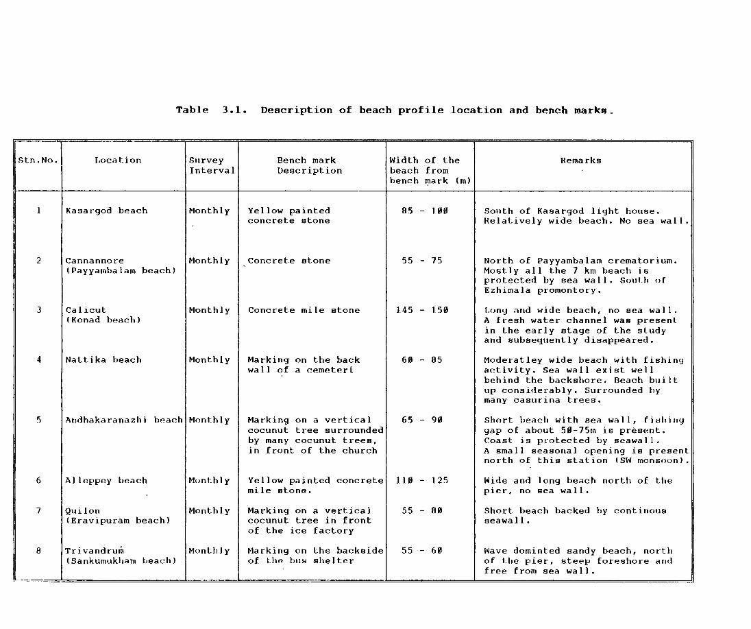
Table 3.1.

stn.No.1 Location I Survey I Interval

1 I Kasargod beach IMonthlY I

2 Cannannore IMonthly (Payyambalam beach)

3 Calicut \Monthly (Konad beach)

4 Nattika beach IMonthly

5 Andhakaranazhi beachlMonthly

6 AIleppey beach IMonthly

7 Quilon IMonthl y (Eravipuram beach)

8 Trivandrum IMonthl Y I (Sankumukham beach)

Description of beach profile location and bench marks ..

Bench mark IWidth of the Description beach from

bench mark

Yellow painted ~188 concrete stone

Concrete stone

Concrete mile stone

Marking on the back wall of a cemeteri

Marking on a vertical cocunut tree surrounded by many cocunut trees, in front of the church

Yellow painted concretel mile stone.

~arking on a vertical cocunut tree in front of the ice factory

Marking on the backsidel of Lhe hus shelter

55 - 75

145 - 159

69 - 85

65 - 99

119 - 125

55 - 89

55 - 69

(m)

I Remarks

South of Kasargod light house. Relatively wide beach. No sea wall.

North of Payyambalam crematorium. Mostly all the 7 km beach is protected by sea wall. South of Ezhimala promontory.

[,ony ilnd wide beach, no sea wa 11 • A fresh water channel was present in the early stage of the study and subsequently disappeared.

Moderatley wide beach with fishing activity. Sea wall exist well behind the backshore. Beach built up considerably. Surrounded by many casurina trees.

Short beach with sea wall, fishing gap of about 59-75m is present. CoasL is protected by seawall. A small seasonal opening is present north of this sLaLion (SW monsoon).

Wide and long beach north of the pier, no sea wall.

Short beach backed by continous seawall.

Wave dominted sandy beach, north of the pier, steep foreshore and free from sea wall.

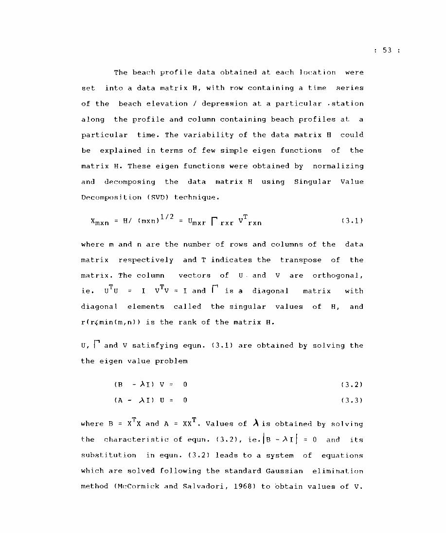
53

The beach profile data obtained at each location were

set into a data matrix H, with row containing i time series

of the beach elevation I depression at a particular .station

along the profile and column containing beach profiles at a

particular time. The variability of the data matrix H could

be explained in terms of few simple eigen functions of the

matrix H. These eigen functions were obtained by normalizing

and decomposing the data matrix H using Singular Value

Decomposition (SVD) technique.

1/2 r T Xmxn = HI (mxn) = Umxr rxr V rxn ( 3.1)

where m and n are the number of rows and columns of the dat.a

matrix respectively and T indicates the transpose of the

matrix. The column vectors of U and V are orthogonal,

ie. = I VTV = I and r is a diagonal matrix with

diagonal elements called the singular values of H, and

r(r<min(m,n» is the rank of the matrix H.

u, r and V satisfying equn. (3.1) are obtained by solving the

the eigen value problem

(B - AI) V -- 0 ( 3 • 2 )

(A - AI) U = 0 ( 3 • 3 )

T T \ where B = X X and A = XX • Values of ~ is obtained by solving

the characteristic of equn. (3.2), ie.IB -All == 0 and its

substitution in equn. (3.2) leads to a system of equations

which are solved following the standard Gaussian elimination

method (McCormick and Salvadori, 1968) to obtain values of V.

54

Knowing V and ~ , U is determined from equn. (3.3).

The ratio between the sum of the squares of the

elements of the factor model and that of the data matrix is

considered as the measure of closeness of the model data

I( -t

Measure of closeness = Z). if ~A i where K is the number of ;= I I = I

factors and r is the rank of the data matrix.

The eigen functions are ranked according to the

percentage of mean square value of the data they explain.

These percentages as accounted by each function, enable

evaluation of the relative importance of each function in

explaining the observed beach variability.

Beach volume computation

To quantitatively estimate the beach volume changes

associated with each of the beaches under study, the relative

changes in volume of the sediments per unit length of the

beach (storage volume) at each location were computed in

cubic metres using an arbitrary defined base line.

3.1.2. Results

In this chapter, the seasonal changes of the beach

morphology inferred from monthly profile data, E.O.F analysis

and storage volume changes at 8 selected beaches are

presented. The storage volume calculated for different months

and different locations are given in Figs. 3.2a & 3.2h.

Kasargod beach

The beach located south of Kasargod light house is a

moderately wide beach backed by cassurina trees. It is free

from any protective structures like sea wall. Three minor

rivers drain into Arabian sea north of this beach. One Major

river Chandragiri having a total annual run-off (3118.6 X 106

3 m (Anonymous, 1974), debouches into the sea within 2 Km

south of the study region. Beach vegetation like casuarina

trees are present on the back shore. This beach falls in the

category of straight open coast beach. The beach has a wide

backshore and a gently sloping foreshore. The width of the

beach varies between 85-100 m, having a berm present at a

distance of 50 -60 m from the bench mark (Fig. 3.1a). The

beach shows maximum variability in the foreshore and it is

almost stable in the backshore region. The beach responds to

the monsoonal forcing with seasonal episodes of erosion and

accretion.

The E.O.F analysis of the profile data shows that, at

Kasargod the first eigen function accounts for 97.5 % of the

mean square value while the second and third accounts 1.5 %

and 0.4 % respectively (Table 3.2)~ In general, the

contribution from the higher order function is insignificant.

Since most of the variations in the profile are accounted by

the first three eigen functions corresponding to largest

eigen values, in the following discussions only the first

three eigen functions are considered.

55

Table 3.2. % Variance explained/contained by each eigen functions.

I FUNCTIONS STi\TION NO.S I

I 1 2 3 4 I

I I

1 I 97.5 1.5 0.4 0.3

") I 99.5 0.2 0.1 0.1 .. I

3 i 99.2 0.4 0.2 0.1 I I

4 I 96.3 2.8 0.5 0.2 I 5 98.2 1.3 0.3 0.1

6 98.1 1.1 0.6 0.1

7 98.6 0.8 0.4 0.1

8 96.5 2.7 0.6 0.1

MEAN GRAIN 92.1 3.9 1.6 1.1 SIZE

The first eigen function (U1), representing the mean

beach profile (Winant et al., 1975) shows a wide backshore

and a berm located between 50-60m from the bench mark with

moderately sloping foreshore (Fig. 3.1c). The associated

temporal function (V1), shows the erosional tendency of the

beach during the period of study.

The spatial configuration of the second function (U2)

indicates the locations of the beach subjected to maximum

va~iabilities. In the present case, the maximum

occured at about 70 m from the bench mark, as

variability

could be

inferred from the peak of the curve. A lesser variability is

seen at about 55 m from the bench mark, coinciding with the

berm crest. In other words, the foreshore region of the beach

undergoes greater changes while the berm is subjected to

lesser variability. The distribution of the second temporal

eigen function (V2) shows the erosional/accretional

to which the beach is subjected. The beach at

experiences a slight accretion from March to April

episodes

Kasargod

followed

by an erosion till September. The erosion has three phases:

an initial rapid rate from April to Mar, a slow rate from May

to August and then again a rapid erosion from August to

September. Then the beach started rapid accretion from

September to December indicating that the beach has regained

some of the material lost due to erosion. Once again, the

beach shows a slight erosion from December to February

followed by an accretional phase towards the end of the

survey.

56

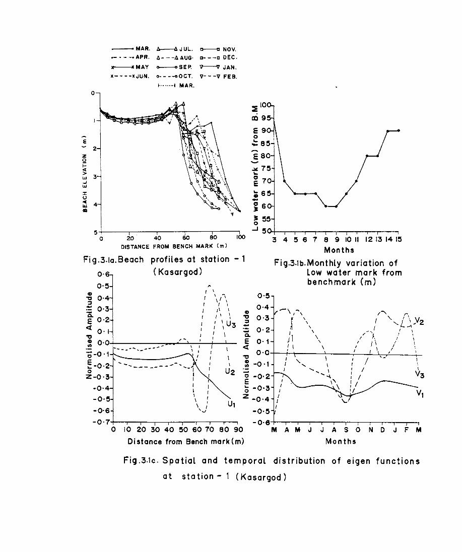
.... e

z 5'2 I-

o

2

~ w 3 ..J W

~ U

~ 4 ID

--_. MAR. A------6.J UL. ct-----1:I NOV.

0- - - -0 APR. 6- - -6 AUG· 0- - -0 DEC.

le -MAY 0 oSEP. v---v .JAN.

x----x.JUN. o----oOCT. v---v FEB .

... .... ·t MAR.

. .

5+---~--~----'-----'---'

cc9

-

o 20 40 60 80 100

DISTANCE FROM BENCH MARK Cm)

Fig.3.la.Beach profiles at station - 1 0.6 ( Kasargod)

0·5

-3 0·4 :I

- 0·3 a E 0·2 et o. I

I I I , I

,. I \

\ -\ I \ I \

" \ I \ \

: \ U3 I \ I ~ ,~

: 0·04------__ ~~-~~-..J--.~--~---' \

-;-0·1 \

~-0.2 --_ ...... _'j U2

Z-0·3 I -0·4 \

-0·5 \ \ I

- 0·6 '''''' U,

0·5

0·4 G ~ 0·3 :J -- 0·2 Q.

E 0·1 et ~

0·0 G -0 ·1 (1) -o -0.2 E ~ -0·3 Z -0.4

-0·5

I

3 4 5 6 7 8 9 10 11 12 13 14 15

Months

Fig.3.1b.Monthly variation of Low water mark from benchmark (m)

I'" 1'\ , I "- ,L ;,.,.Y2 , , I ,

',\ I \

\ I" I, I \ I \ ,

I I \ / \ \ / \

I \ / I I

/ ~.

\ \ .... \

V3

- 0 . 7 - O· 6-+-.......... ~---..--..--...--.......-.......... --.----r-.----..... o 10 20 30 40 50 60 70 80 90 M A M J J A SON 0 J F M

Distance from Bench mark (m) Months

Fig.3.1c. Spatial and temporal distribution of eigen functions

at sta tion - 1 (Kasargod)

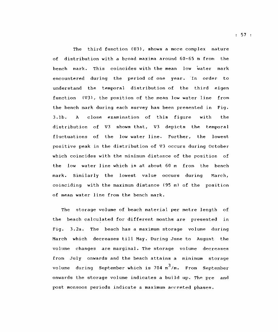
The third function (U3), shows a more complex nature

of distribution with a broad maxima around 60-65 m from the

bench mark. This coincides with the mean low water mark

encountered during the period of one year. In order to

understand the temporal distribution of the third eigen

function (V3), the position of the mean low water line from

the bench mark during each survey has been presented in Fig.

3.1b. A close examination of this figure with the

distribution of V3 shows that, V3 depicts the temporal

fluctuations of the low water line. Further, the lowest

positive peak in the distribution of V3 occurs during October

which coincides with the minimum distance of the position of

the low water line which is at about 60 m from the bench

mark. Similarly the lowest value occurs during March,

coinciding with the maximum distance (95 m) of the position

of mean water line from the bench mark.

The storage volume of beach material per metre length of

the beach calculated for different months are presented in

Fig. 3.2a. The beach has a maximum storage volume during

March which decreases till May. During June to August the

volume changes are marginal. The storage volume decreases

from July onwards and the beach attains a minimum storage

volume during 3 September which is 704 m Im. From September

onwards the storage volume indicates a build up. The pre and

post monsoon periods indicate a maximum accreted phases.

57

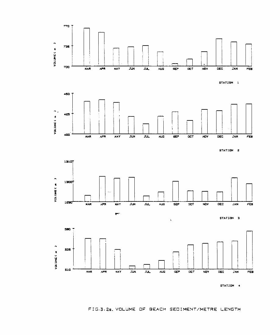
, III

~ ..J Q >

!

~ ..J Q >

I

!

-r--

- - -- r--r--

r-- -~ n .

MAR MAY JUN JUL AUG SEP acT NaY CEC J'AN

STATION

450

- r-- - r-- r--

- -r--

- ~

r--

n MAR MAY JUN JUL AUG SEP OEC J'AN

STATION 2

STATION 3

sas

510 ~ __ ~ __ ~ __ ~~ __ ..J-~ __ ~.....J __ .....J __ ~ __ ~~ __ ~~ __ ~ __ ~.....J __ ~ __ ~~ __ ~.....J __ .....J--..J

MAR APR MAY J'UN JUL. AUG SEP acT NaY !lEC JAN FEe

STATIDN 4

FIG.3.2a. VOLUME OF BEACH SEDIMENT/METRE LENGTH

PAYYAMBALAM BEACH

The Payyambalam beach at Cannanore is situated about 5

km south of Ezhimala promontory. Valapattanam river with an

annual run off of 2764.9 X 106 m3 drains in to the sea about

10 km north of this beach. It is a short beach (7 km),

protected by sea wall. The upper backshore 1S covered by

beach grass. The beach has a moderately steep foreshore and

gentle backshore with a total width of 55-75 m. From the

profiles (Fig. 3.3a), it is clear that the beach has a stable

backshore while the foreshore is subjected to

seasonally.

changes

The mean beach function (Ul) shows a narrow backshore

with a well developed berm and a moderately sloping foreshore

with a step like feature at 20 - 30 m from the ·bench mark.

(Fig. 3.3b). The corresponding temporal eigen function (Vl)

shows almost stable nature of the beach during the study

period. The second function U2 indicates maximum variability

in the upper foreshore where the step-like feature is

noticed. The distribution of the second temporal function

(V2) shows that the beach is subjected to continuous erosion

from Marc~ till July with a high rate of erosion during June­

July. Thereafter the beach starts building up rapidly,

regaining its lost material till December. Once again the

beach undergoes erosion from December to till the end of the

survey. The third spatial function (U3) shows a maximum

around 40-45m from the bench mark. The lowest positive peak

associated with the third temporal function occurs during

58

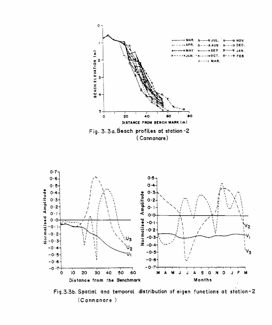
o

.... E

z2 o .... ~ ~ 3 ... :t: c.J Cl[

... 4 ID

_e MAR. A---A J UL. o---a NOV.

,- - - -. APR. A- - -4 AUG; D- --D DEC.

" IIMAY _SEP.

11- - - -11 JUN .• 0- - --oOCT.

, ....... , MAR.

V-V JAN .

V- - -V FEB.

5~,--~--~--~--~--~~~~~~~

o 20 40 60 80

DISTANCE FROM BENCH MARK (m>

Fig. 3.3 a. Beach profiles at station-2 ( Cannanore)

0·7

0·6 , ..... I \

o· ~ I ~ 0·4 I \.~ :I I '\' .. 0·3 ,,' \ '. Q. I " \ \ E o· 2 I' \ \

A : \ " "" 0'1 I

,: \ \ ~ O.04-~----~~/-?r~~----~~-----. \ ~-O'I \ \ o , , E-0'2 ,'. loo o ' 'U~ 2- 0 '3 " ~ ,

-0,4 U2

\

-O·~ U, -0,6

-0-7'4---~--~--~--~--~--~

o 10 20 30 40 ~O SO

... · (:~, ." , \ .",,\ ~, , ..... , I I l' I - , ",.."" ,

._ • I I \ /,. I '\ ,

- ',,' \ I I , I. I , E ", \ \ J~ \/. \ 1

- ':' \ I, \ I, - O·~------~--~~--~~------~~ \ / , ." : / \ I \1

• I \ /' I " • \ ' 1V .- : \ / " I 2 c; -O· 2 I I" I E 10.--__, 1

_ -0.3 '. ___ ~_...r-_-'~----~I VI o ' I / , Z -0.4 '-- I I

, I I -0· , I

-0,6 I I v

-0·7'~-r~--~~~~--~~~~--~

V3

M A M J J A S O' N 0 J F M

Distance from the Benchmark Months

. Fig.3.3b. Spatial and temporal distribution of eigen functions at station-2

(Cannanore )

July coinciding with the nearest position of the low water

mark at about 35 m from the bench mark. The lowest value

during March-April coincides with the farthest position of

mean water line which is 55 m from the bench mark during

March.

The storage volume of beach material for this location

(Fig. 3.2a), indicates that the beach does not undergo much

changes from March to May while during July to October, it

gains material. The lowest storage volume level of the beach

is during July (412 m3/m). From July end to September beach

experiences accretion and receives some part of the lost

material. From September end, the beach once again passes

through a state of erosion till the.end of October and again

shows a building up tendency. In general the storage volume

shows that the beach loses material during monsoon months of

June-July and regains the materials during the rest of the

year except an erosional tendency during October (416.6m 3 /m).

KONAD BEACH

Konad beach at Calicut is a long and very wide sandy

beach free from any protective structures like sea walls. A

fresh water channel was present in the early stage of the

study which has been subsequently disappeared. There are two

small rivers, on either side of the beach, Elattur river on

the south and Kallai river on the north. The beach width

varies between 145-150 m from the bench mark. From the beach

59

profiles (Fig. 3.4a), it is clear that the beach profile

variations are the least for this beach as compared to the

other 8 locations.

The first spatial function (Ul) shows that the beach

has a very wide gently sloping backshore and a moderately

steep foreshore (Fig. 3.4b). The backshore contain two berms,

one at 30-40 m which is a permanent berm while the other at

120-130 m is a seasonal one. The almost straight line of the

distribution of the temporal function (VI) associated with

the first eigen function, shows the stable nature of the

beach during the period of study. The spatial configuration

of the second function (U2) shows the maximum variability

associated with the second berm and lesser variability at

100-1]0 m from the bench mark. The second temporal eigen

function (V2) shows that the beach undergoes an initial slow

accretional phase during March-April followed by an eroding

phase till the end of June. From July 'onwards the beach

started building up at a very slow rate till January. The

maximum value associated with the third spatial function (U3)

around 140 m from the bench mark indicates the ·position of

low water mark. Its corresponding temporal function (V3)

shows lowest positive peak during January-February at 145 m

which indicated the farthest position of the low water line

while the lowest value at 30-35 m during November-December

indicates the closest position of the mean low water line

from the bench mark.

60

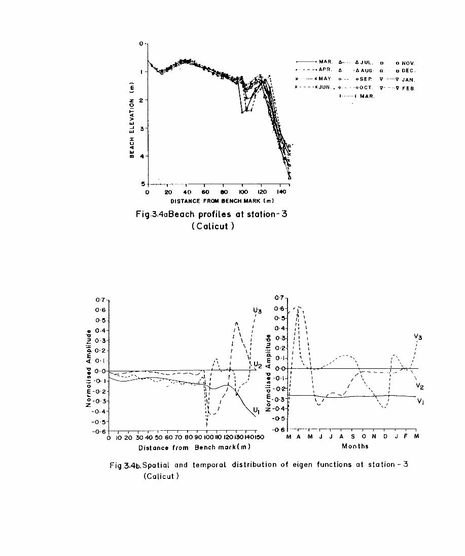
o

E

z 2 o !« > .... ~ 3 l: U .. .... m 4

o 20 40 60 eo 100 120 140

DISTANCE FROM BENCH MARK (m)

Fig.3.4aBeach profiles at station- 3 ( CaLicut )

0·7

0·6

~. MAR. 6-·-6 JUl. 0--0 NOV .

• -- - - -.APR. 6- - -6 AUG· 0- ---0 DEC.

__ -_MAY o·--··oSEP. "'·-··--9 JAN.

x----xJUN .• o----oOCT. 9----9 FEB.

, ...... , MAR.

- 0.6 -() R+--r-r-..---.--,--r---r--.----,.---,.....---r--~ o 10 20 30 40 ~O 60 10 BO 90 100110 120 130 1401~ M A M J J A SON 0 J F M

Distance from Bench mark( m) Months

Fig.3.4b.Spatial and temporal distribution of eigen functions at station - 3

(Calicut)

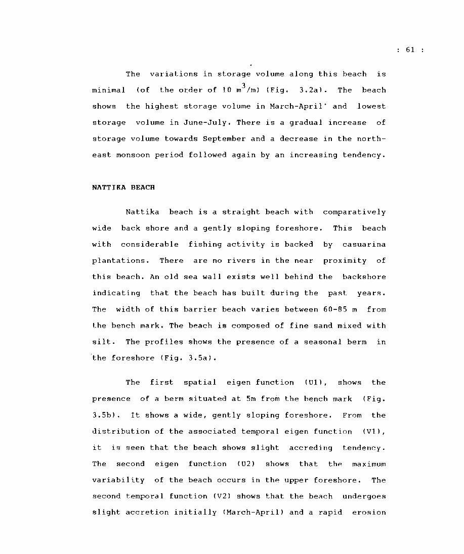
The variations in storage volume along this beach is

minimal (of the o~der of 10 m3 /m) (Fig. 3.2a). The beach

shows the highest storage volume in March-April" and lowest

storage volume in June-July. There is a gradual increase of

storage volume towards September and a decrease in the north­

east monsoon period followed again by an increasing tendency.

NATTIKA BEACH

Nattika beach is a straight beach with comparatively

wide back shore and a gently sloping foreshore. This beach

with considerable fishing activity is backed by casuarina

plantations. There are no rivers in the near proximity of

this beach. An old sea wall exists well behind the backshore

indicating that the beach has built during the past years.

The width of this barrier beach varies between 60-85 m from

the bench mark. The beach is composed of fine sand mixed with

silt. The profiles shows the presence of a seasonal berm in

the foreshore (Fig. 3.5a).

The first spatial eigen function (U1), shows the

presence of a berm situated at 5m from the bench mark (Fig.

3.5b). It shows a wide, gently sloping foreshore. From the

distribution of the associated temporal eigen function (Vi),

it is seen that the beach shows slight accreding tendency.

The second eigen function (U2) shows that the maximum

variability of the beach occurs in the upper foreshore. The

second temporal function (V2) shows that the beach undergoes

slight accretion initially (March-April) and a rapid erosion

61

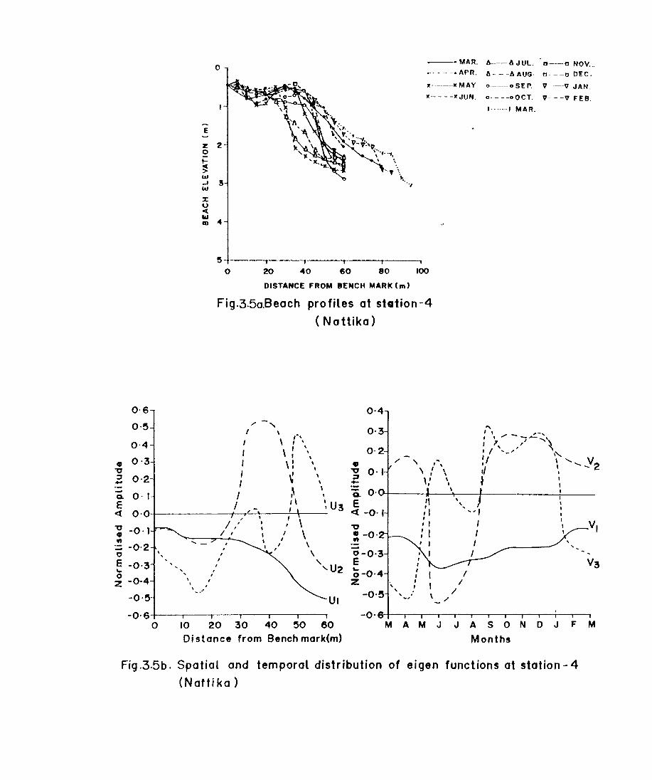
0·6

0·5

0·4

Cl 0·3 'tJ ::r 0·2 .... Q. 0·' E <t 0·0 'tJ -0 ·1 Cl wt

-0,2 ., \ , E '-

-0·3 0 z -0-4

-0,5

-0'6 0

, , , •

'0

~

e

z 0 t-C > ... -' ... :t: 0 C 1&1 III

'-

, , I ,

\ , ."

o

2

'., \. 3 ~.

At

.,

__ e MAR. A--A JUl. D---I] NOV ...

.----.Arn. A---AAUG· D---O DEC.

11------11 M AY 0--·---0 SE r. '1----'1 JAN.

x----xJUN. o.---oOCT. '1---'1 FEB.

, ....... , MAR.

5~-----'------T------r------r-----~

o 20 40 60 80 100

DISTANCE FROM BENCH MARK (m)

Fig.3.5a.Beach profiles at station-4

(Nattika)

0·4 ",- '" I 0·3 \

\ ,-,

I I ' , , 0·2 I \ , , ,

I \ : , • ,,- , , "0 \ I ~

, ;:, I \ -~

I o· I • Q.

/ ' \ " U3 E I et -0,' ,

\ I,' "0 / , , \ :: -0' ,

\ , --, \ 0-0·3 I , E

'U2 ::; -0'4 Z "

\,

-0'5 \, \ U, ~,

-0'

" , \

I , "... - -.....!.:::" ", ,,' \ I I '-" i'" , ' ,I I '-_ V2 I 1-... I ,

~ , I

, I

V, , I

V3 I

/ / ,,-

20 30 40 50 60 M A M J J A S 0 N 0 J F M Di stance from Bench mark(m) Months

Fig .3.5b. Spatial and temporaL distribution of eigen functions at station - 4 (Naffika)

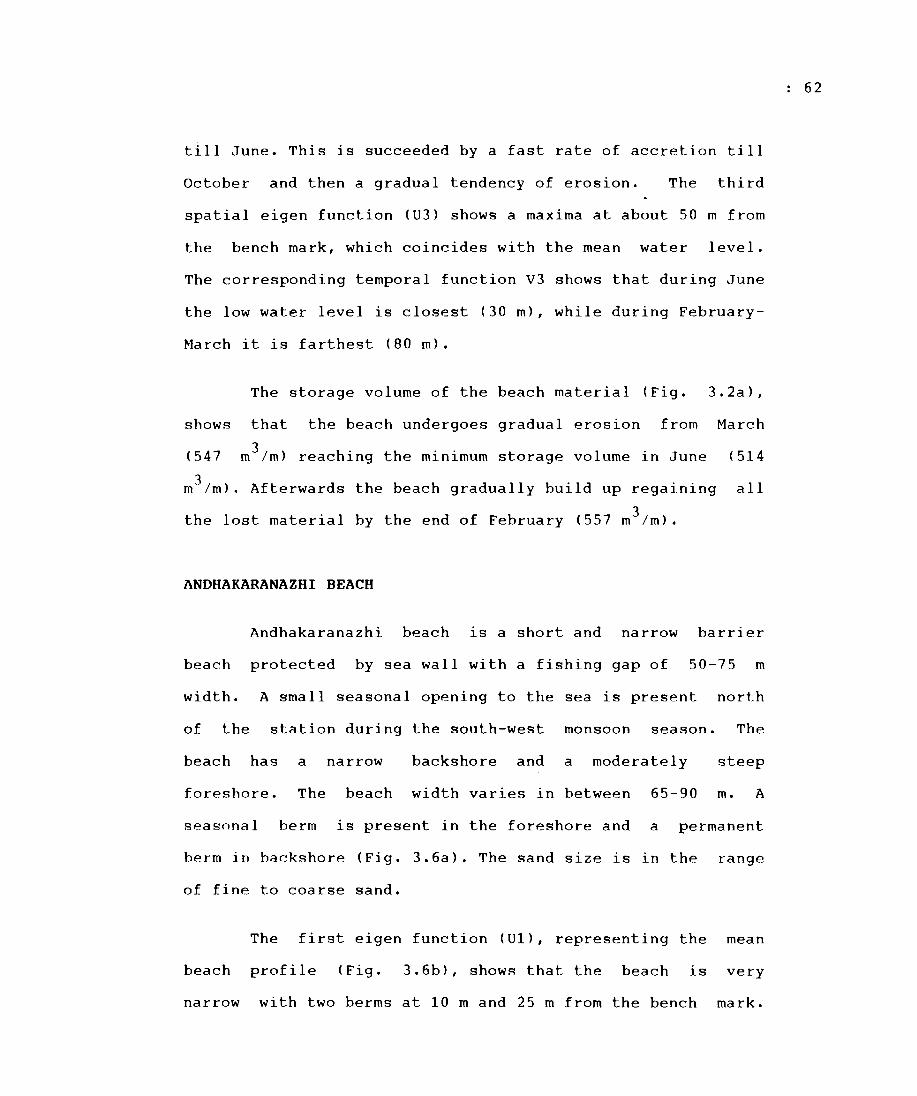
till June. This is succeeded by a fast rate of accretion till

October and then a gradual tendency of erosion. The third

spatial eigen function (U3) shows a maxima at about 50 m from

the bench mark, which coincides with the mean water level.

The corresponding temporal function V3 shows that during June

the low water level is closest (30 m), while during February­

March it is farthest (80 m).

The storage volume of the beach material (Fig. 3.2a),

shows that the beach undergoes gradual erosion from March

(547 m3 /m) reaching the minimum storage volume in June (514

m3/m). Afterwards the beach gradually build up regaining all

the lost material by the end of February (557 m3 /m).

ANDHAKARANAZHI BEACH

Andhakaranazhi beach is a short and narrow barrier

beach protected by sea wall with a fishing gap of 50-75 m

width. A small seasonal opening to the sea is present north

of the station during the south-west monsoon season. The

beach has a narrow backshore and a moderately steep

foreshore. The beach width varies in between 65-90 m. A

seasonal berm is present in the foreshore and a permanent

berm in backshore (Fig. 3.6a). The sand size is 1n the range

of fine to coarse sand.

The first eigen function (Ul), representing the mean

beach profile (Fig. 3.6b), shows that the beach is very

narrow with two berms at 10 m and 25 m from the bench mark.

62

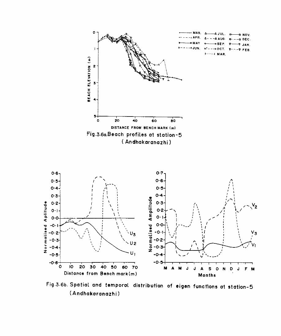
0'6

o·~

0·4

0'3

• 0·2 ~ ~ 0'1 .. Q. o· et ~ -0·1

" .!! -0-2 -0 E -0'3 ..

-0-4 0 z

-o·~

-0,6 0

I

I

10 20

o --_. MAR. A----4 J Ul. D---O NOV. .- - - .-. APR.

11 IIMAY

x----ICJUN.

-E

z 2 0 ~

~ .... ..J S .... X (J C ....

~. ID

,+-----~~-----r------._----~r__, o 20 40 60 eo

DISTANCE FROM BENCH MARK (m)

Fig.3.Ga.Beach profiles at station-5

( Andhakaranazhi)

0·7 ,.-I " 0'6

\-- ... , , o·~ " \

I : I .

I 0·4 I , • I I ~

I \ ::J 0'3

\ I -I I

\ "\ I Q. ,.

\ '. E \ ./ . t\ I \ , \

f \ \ ,

\ \ Cl I , , \ \

, , -... I I

\

~ o· \ ' -' • , \

\ ., \ "

\ \ U3 .... \ I , -' , , \. , ..... U2 \ , , ,

" U,

-0' 30 40 SO 60 70 M A M J J A

1I---IIAUG· D---D DEC.

~SEr. V-V JAN.

o!---oOCT. V---V FEB.

1·······1 MAR.

" I, I , I , I , , ,

I , ,,, .... I

I \' V, \ /- 2 /I / '\

/ ,'-./ ,

-- , "" ,

( , , , , V3

I

"

S 0 N 0 J F M Distance from Bench mark(m) Months

Fig.3.Gb. Spatial and temporal distribution of eigen functlons at station- 5 (Andhakaranazhi)

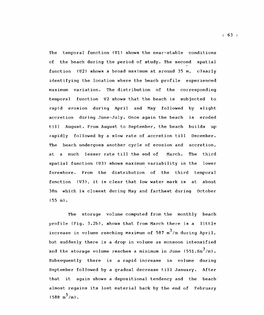
The temporal function (VI) shows the near-stable conditions

of the beach during the period of study. The second spatial

function (U2) shows a broad maximum at around 35 m, clearly

identifying the location where the beach profile experienced

maximum variation. The distribution of the corresponding

temporal function V2 shows that the beach is subjected to

rapid erosion during April and May followed by slight

accretion during June-July. Once again the beach is eroded

till August. From August to September, the beach builds up

rapidly followed by a slow rate of accretion till December.

The beach undergoes another cycle of erosion and accretion,

at a much lesser rate till the end of March. The third

spatial function (U3) shows maximum variability in the lower

foreshore. From the distribution of the third temporal

function (V3), it is clear that low water mark is at about

30m which is closest during May and farthest during October

(55 m).

The storage volume computed from the monthly beach

profile (Fig. 3.2b), shows that from March there is a little

increase in volume reaching maximum of 587 m3 /m during April,

but suddenly there is a drop in volume as monsoon intensified

and the storage volume reaches a minimum in June (551.6m3/m).

Subsequently there is a rapid increase in volume during

September followed by a gradual decrease till January. After

that it again shows a depositional tendency and the beach'

almost regains its lost material back by the end of February

(588 m3 /m).

63

r-- r-

r- r- r-- r-r-

r-

I

n .--. n n ~AR Af"R ~AY JUN JUL AUG SEP OCT NOV OEC .rAN FEa

S50

STATION 5

970 -r--

r-- r-- r--r-- r-- r--

! r- r--

I""""""

Ii sac

~AR APR ~AY .ruN JUL AUG OCT NOV CEC .rAN FEa

STATION 5

•

STATION 7

r--r-- r-

r- r--r--

r-,..- r--

43S I r--...

101 X ~ .J a > 380

n n ~AR APR MAY .ruN JUL AUG SEP OCT NOV OIiC .rAN

STATION S

~IG.3.2b. VOLUME O~ BEACH SEDIMENT/METRE LENGTH

ALLEPPEY BEACH

The beach at Alleppey is a wide and long barrier beach

situated south of Alleppey pier and is free from any

protective structures. There are no rivers in the proximity

of this beach. The width of the beach ranges between 110-125

m. The beach is composed of fine size sands. The profiles

(Fig. 3.7a), show a stable backshore and a foreshore which

gets

bank

season

built up even during the peak monsoon months. The mud

occurring in this region during the south-west monsoon

(Kurup, 1977; Kurian et al., 1984, 1985) dampens the

high monsoonal waves and makes this nearshore region very

calm. The observed accretion of the beach during the monsoon

months is brought in by the presence of the mud bank.

The distribution of mean beach function (Ul) shows the

presence of a very wide backshore and a gently sloping

foreshore (Fig. 3.7 b). A seasonal berm is situated at 80 m

from the bench mark. The associated temporal function (VI)

shows an overall accretional tendency of the beach. The

second spatial function (U2), shows a maximum near the lower

foreshore where the beach undergoes large variations. The

temporal function (V2) shows that the beach is subjected to

accretion throughout the period of study except during May­

June, September-October and February-March. The distribution

of the third spatial function (U3), shows the position of

mean low water mark at 90 m from the bench mark. The third

temporal function (V3) shows that the mean water line

fluctuates between 90 m during May and 110 m during November.

64

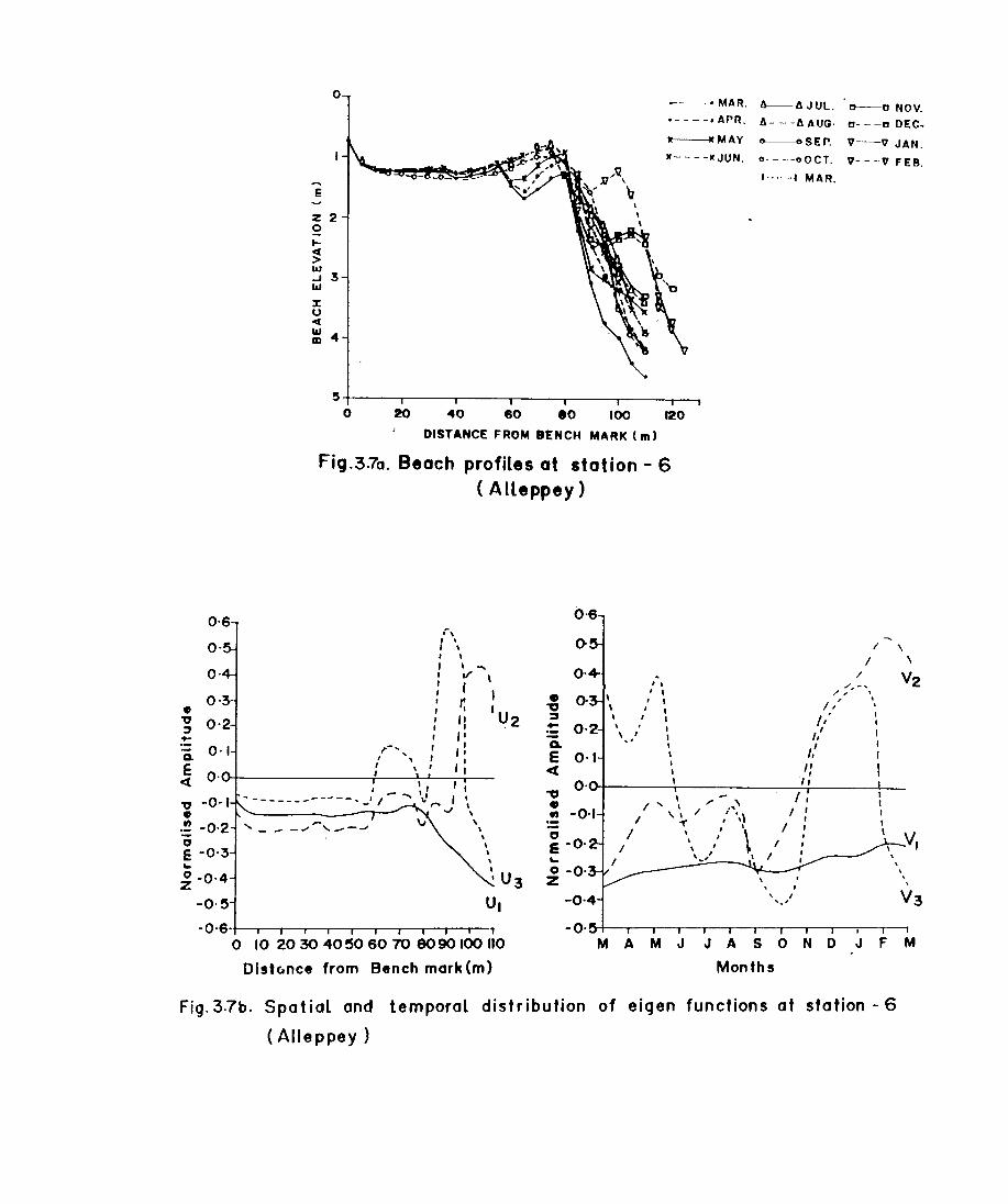
Cl ~ :::I +-

Q.

E « ~ Cl fI

" E ~

0'6

O'

O·

O·

-0,2

-0,3

0-0·4 Z

-0,5

o

E

z 2 o I-

~ W ..J 3 w

l: U ~

:;: 4

~. MAR. A-----Il JUL. D---O NOV .

• - - - -. ArR. L\ - - -A AUG: 0- - -0 DEC.

--MAY O-----(tSEF'. V-V JAN.

x----xJUN. o----oOCT. v---v FEB. , ....... , MAR.

~T-----.----,r----,-----.-----.----,--, o 20 40 60 80 lOO 120

DISTANCE FROM BENCH MARK ( m)

Fig.3.7a. Beach profiles at station - 6

.-, , \ , \ , , , , , II' I f

( AlLeppey)

b'6

()

O· -, I

• , I

I

/

, , , ,

,I I 'lJ

() , I , I

, I

/"" -, ", , , , /1

" - - -.,,""',.,,--,

r', ' , " : "

,. , 'I I , I , :

, , \! , , , ,

\ \ \ \ \ , 'U3

UI

~ --Q,

E et

~ O'

• ~ -0 e -0'

\ • I

',.' I /" ,,'

I I I I I

,,I , : I,

\ ,., / I

I "', \ / /\, I : / .,.. \ I'

/ '.,' \ / \,' ~ I

I ,_" I

, , , , ,

'.'

VI

-0,6 , o 10 2030 40506070 8090 100 110

Dist6nce from Bench mark (m)

M A M J J A SON 0 J F M

Months

Fig.3.7b. Spatial and temporal distribution of eigen functions at station - 6

(Alleppey)

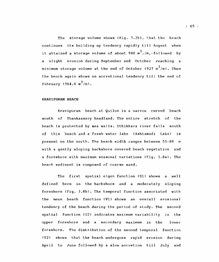
The storage volume shows (Fig. 3.2b), that the beach

continues its building up tendency rapidly till August when

it attained a storage volume of about 940 m3 ./m,.followed by

a slight erosion during September and October reaching a

minimum storage volume at the end of October (927 m3 /m). Then

the beach again shows an accretional tendency till the end of

3 February (964.6 m Im).

ERAVIPURAM BEACH

Eravipuram beach at Quilon-is a narrow curved beach

south of Thankassery headland. The entire stretch of the

beach is protected by sea walls. Ithikkara river falls south

of this beach -and a fresh water lake (Ashtamudi Lake) lS

present on the north. The beach width ranges between 55-SO m

with a gently sloping backshore covered beach vegetation and

a foreshore with maximum seasonal variations (Fig. 3.Sa). The

beach sediment is composed of coarse sand.

The first spatial eigen function (U1) shows a well

defined berm in the backshore and a moderately sloping

foreshore (Fig. 3.Sb). The temporal function associated with

the mean beach function (V1) shows an overall erosional

tendency of the beach during the period of study. The second

spatial function (U2) indicates maximum variability in the

upper foreshore and a secondary maximum in the lower

foreshore. The distribution of the second temporal function

(V2) shows that the beach undergoes rapid erosion during

April to June followed by a slow accretion till July and

65

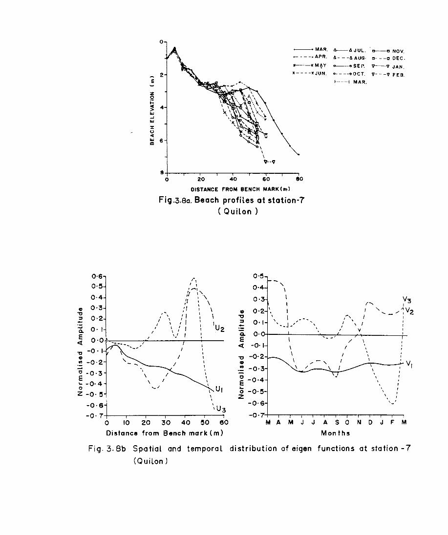
o·s O·~

0·4

0·3

0·2

E

z 2 ~

0

2

---MAR.

.- - - -. APR.

Jf---II M~Y

x- - - -XJUN.

~ 4 1&1 ...J 1&1

J: U « 1&1 ID

6 \ \ \ tr-9

8 , 0 20 40 60 80

DISTANCE FROM BENCH MARK (m)

Fig .3.80. Beach profiles at station-7 (Quiton)

,., I ,

,'"", " " '\

if \ " I I \

,', 'I ~ \ I I " I I

O·~

0·4

O·

"\ \

I

, ,

1\---1; JUL.

4- - -4 AUG·

~SEr.

0- - --oOCT.

I·······!

~,

I ,

MAR.

I ,I I

~ NOV. 0- --0 DEC.

V-V JAN.

"1- --v FEB.

/ I \" I : 'U2 I V ~ O'~----~------~--~---T~--------~ If I :

O'O~~---,~----r-~---

Q. O· I E et

E ........ " <{

/ I

~ -0'1 «)

In -0,2 ~

o -0,3 E ~ -0,4 o Z -0' ~

-0,6

,---'

\ I

\U3 -0'7+---r-~--r--~---r--'

o 10 20 30 40 ~O 60

Distance from Bench mark (m)

~ ., Cl) -0,3

E -0,4 ... o -O·~­Z

-O·s

, \

I I

f , I

, \

\ , '-

, I

I

-0·7'~-.-.r-.--.~-~-r~-.-'--r-'

MAMJJ ASONDJFM

Months

Fig- 3. 8b Spatial and temporal distribution of eigen functions at station -7

(QuiLon)

erosion during August to September. Subsequently the beach

builds till December and shows an erosional trend during

December-January. The third spatial eigen function (U3) shows

the position of the low water mark at 60 m. The corresponding

third temporal function (V3) indicates the closest water mark

at 30 m during June and farthest at 60 m during February.

The storage volume shows that the beach has a maximum

storage volume in April (425.4 m3 /m), (Fig. 3.2b) and a

minimum storage volume in June (371 m3 /m) followed by a

slight building up during July-August and erosion during

September (373.6 m3/m). This is followed by an accretional

trend during October-December. In general, the beach loses

material over a period of the year.·

SHANKUMUKHAM BEACH

Shankumukham beach at Trivandrum situated north of the

Valiyathura pier is a sandy beach with comparatively wide

backshore and is devoid of any beach vegetation. Among all

the beaches studied, this beach is exposed to higher wave

energy throughout the year and undergoes maximum profile

changes (Fig. 3.9a). The beach has a gently sloping backshore

and a very steep foreshore during the rough weather season.

The beach has a width of 55-60 m and is composed of coarse

sized sand.

The distribution of the mean beach function (Ul) shows

a berm at 20 m from the bench mark and a moderately sloping

66

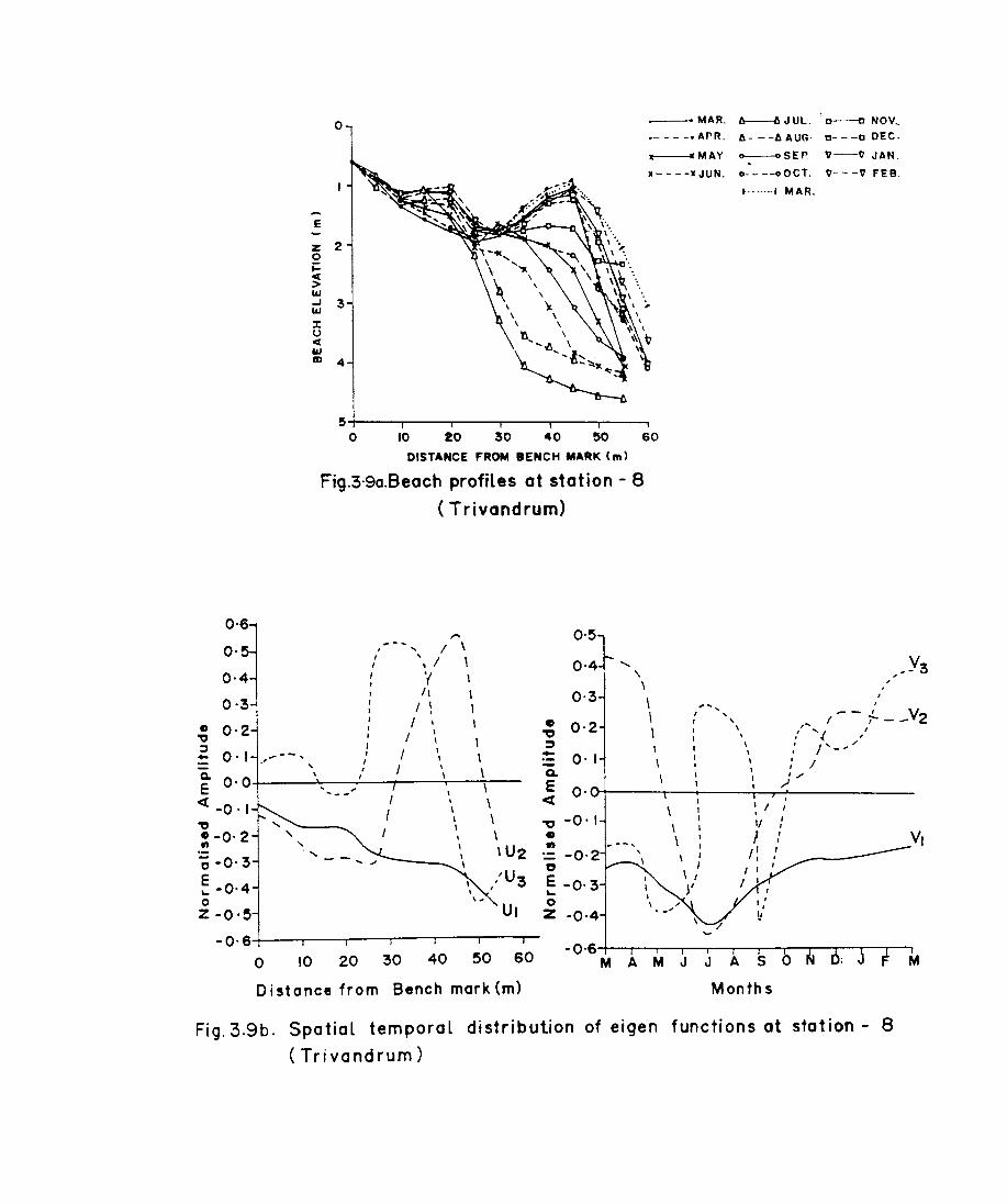
0

E

z 2 o ~ Cl > 1&1

kl 3 :J: (.)

Cl 1&1 CD 4

~·MAR.

.----.Af'R.

x------IC M AY

------JUN.

5+----,r----r----.----.----~--~

o 10 20 30 40 50 60

DISTANCE FROM BENCH MARK (m)

Fig.3·9a.Beoch profiLes at station - 8

( Trivondrum)

0·6

O·~

0·4

0·3

.. 0·2 " :I - 0·1 ---, .'

I I

I I

,.. , / \ " / \ .{

I, I I \ I

I I' I ; 1 I

, " I I Ci O.O+-----~----~,'---r'----~\r---~\----E ~ __ " \ \ <t -0 . I I \ \ " I \ \ : -0· 2 "" \ '0 -0· 3 " .... -' \ U2

~ -0·4 o Z -O·~

\ \ \.

UI

0.5}

0·4 " , \

0·3 .,

0·2 "0 ::J - 0·1 ~

E o· et "0 -0·1 ., ., .--, - -0·2 o E -0.3 ~

o Z -0·4

\ \ \ , ,

\

, \

6---lI JUL.

6- - -Il AUG· __ SEf'.

0- - --oOCT.

1·······1

I I ,

MAR.

[t--tI NOV ..

D- --D DEC.

v-v V- --V

JAN.

FEB.

, I

v _ - 3

VI

-0·64---~--~--~----.---.----r-

40 50 60 -0·6~~--r-~~~~~~~--~~~~

o 10 20 30 M A M J J

Distance from Bench mark (m) Months

Fig.3.9b. Spatial temporal distribution of elgen functions at station - 8

(Trivandrum)

foreshore (Fig. 3.9b). The corresponding time dependent

factor, (Vl) indicates an annual accretional trend. The .

spatial configuration of the second eigen function (U2) shows

maximum variability in the lower foreshore and lesser

variability near the berm. The second temporal function (V?!

shows rapid erosion from April to July followed by rapid

accretion till October. The accretional trend continues till

Decemher at a much reduced rate. However from December till

the end of February, the beach does not undergo much

variations. The distribution of the third spatial function

(U3) indicates that the position of the low water level is

around 35-40 m from hench mark where maximum erOS1on occurs.

Its corresponding temporal function (V3) shows that the

closest position of mean low wat~r level occurs during July

(30 m) and is farthest during September (55 m).

The storage volume computed for this beach (Fig.3.2b)

shows that the beach loses material from April reaching a

minimum storage level in July (400 m3 /m). Subsequently the

beach experiences gradual accretion leading to a considerable

deposition till the end of February when the beach gets built

up considerably. The response of this beach depicts the

typical monsoonal response of an open coast beach undergoing

rapid erosion under monsoonal high waves taking away the

beach material at a faster rate and regaining the material

over longer period through the fair weather period.

67

3.2. Beach sediments

The beach is made up of unconsolidated sediments which .

range from very fine sands to pebbles. Wind, waves and tides

are the important factors responsible for the movement of

materiai on the beach and the resultant sediment distribution

(Komrlr, 1976). The difference in wave energy and the period

of the ocean swell are important factors that determine the

nature and distribution of the foreshore sediments. The

variation in grain size for any type of beach is primarily a

function of variation in wave height and to a lesser degree,

the wave period. (Write et al., 1985). On a beach, sediment

is mainly exposed to two forces of unequal strength acting in

opposite directions - the incoming waves and the outgoing

wash. This is the primary mechanism by which sediment get

sorted. The textural parameters, in addition to the degree of

sorting, also reflect the mode of transportation and the

energy levels of transportation media.

The aim of the present investigation is to determine

statistically the significant variations 1n grain size

distribution of the beach sediments along different beaches

under study. In order to get a comprehensive picture about

the seasonal changes in the size characteristics of the

sediments along all the beaches, average moment measure

statistics viz. mean, standard deviation and skewness were

computed. The analysis has been done only for the samples

collected from the low waterline.

68

3.2.1. Materials and methods

Monthly beach sediment samples were collected over a

period of 12 months from each station, close to the water

line during spring low water level when the beach exposure

was maximum above the water line. A total of 104 samples

were collected and used for the present study. The samples

represent top 5 cm as on the day of sampling. Sieve analysis

was carried out to study the grain size distribution.

Grain size analysis

Beach samples were subjected to size analysis by the

simple sieving method. The samples were collected by scoop

sampling. Approximately 1 kg in weight was washed free of

salt, silt and clay and finally oven dried. From that 100 gm

was separated by the conning and quartering method. Shells

and shell fragments, if any present in the samples were

separated by hand-picking method, as the presence of this

would distort the trend of analysis. The samples were then

sieved for 15 minutes in a semi automatic, motor driven

mechanical Ro-Tap sieve shaker using a set of standard ASTM

sieves (mesh nos. 18, 25, 35, 45, 60, 80, 120, 170 and 230).

The weight of each fraction representing a particular grain

size was measured using an electronic balance. The graphic

mean, median, standard deviation and skewness were calculated

based on the formula of Folk and Ward (1957).

69

E.O.F of grain size data

Mean grain size data of each 'of the samples were

further subjected to E.O.F analysis to understand the spatio­

temporal variability of the sediments in different

environments. The size distribution of all the 104 samples

were represented in the form of a matrix, L(X,~) of discrete

size class with X as the location and~, the grain size

class. The matrix was converted to a normalized data matrix,

X(X,~) and the eigen functions were obtained as described in

section 3.1.2.

3.2.2. Results

The monthly variation of graphic mean, standard

deviation and skewness calculated for the samples from

different location are presented in Figs. 3.10a & 3.10b for

mean size, Figs. 3.11a & 3.11b for standard deviation and

Fig. 3.12a & 3.12b for skewness.

At Kasargod (Fig. 3.10a), the mean ,size of the beach

sands fluctuated generally between 0.22 mm to 0.94 mm which

corresponds fine to coarser grade. During the south-west

monsoon period (June to September), the sediment is mostly in

the coarser sand class. Fine and medium grade sands are

present during the other months. On an average, the mean

grain size of the beach is of the medium sand size. The

standard deviation values (Fig. 3.11a), reveal that majority

of the water line samples are moderately sorted and display

70

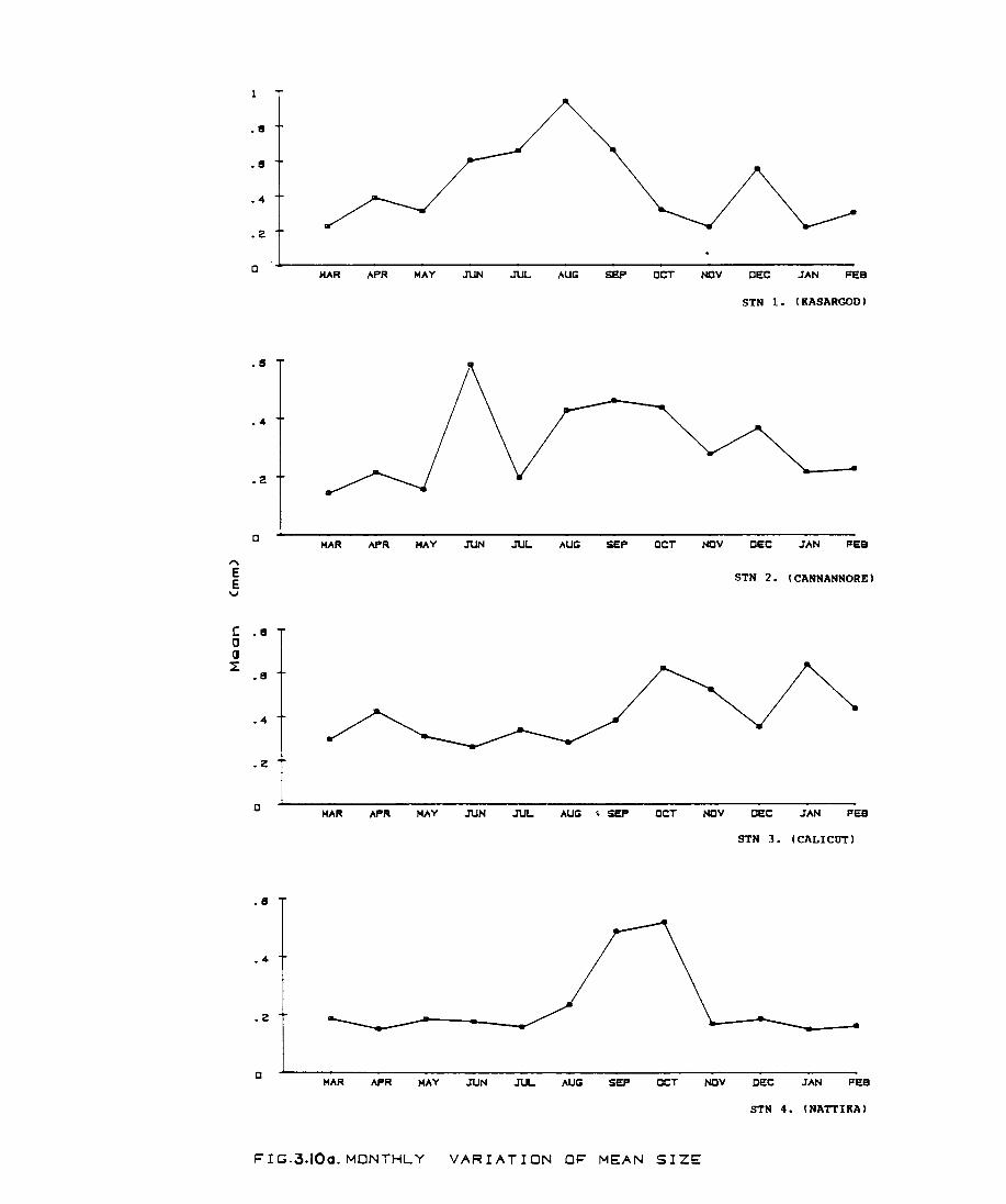
.8

.5

.4

.2

a MAR APR MAY JUN JUL AUG SEP OCT NaV DEC .1AN FEe

STN 1. (KASARGOO)

.5

.4

.2

a MAR APR MAY JUN JUL AUG SEP aCT NOV DEC .1AN FEe

" E STN 2. (CANNANNORE) E v

C .8 0 (J

~ .5

.4

.2

a MAR APR MAY JUN JUL AUG SEP aCT NaV DEC .1AN FEe

STN 3. (CALICUT)

.5

.4

.2

o MAR APR MAY JUN JUL AUG SEP OCT NOV DEC .1AN FEe

STN 4. (NATTIKA)

F I G.3.IOa. MONTHLY VARIATION OF MEAN SIZE

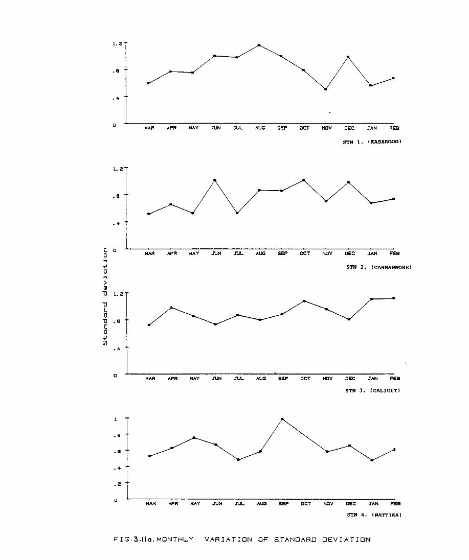
1.2

.11

.4

a MAR APR MAY JUN JUL AUG SEP OCT NOV DEC .rAN FEB

STH 1. (KASARGOO'

1.2

.11

.4

C a 0 MAR APR MAY .ruN JUL AUG SEP aCT NOV DEC .rAN FEB .... +' STH 2. (CANNANNORE' a .... > (J

11 1.2

11 L a

11 .11 C a +' (/)

.4

a APR MAY JUN JUL AUG SEP aCT NOV DEC .rAN FEB

STH 3. (CALICOT'

1

.11

.S

.4

.2

a MAR APR MAY JUN .ruL AUG SEP aCT NOV DEC .rAN FEB

STH 4. (NATTIKA)

FIG·3.lIa. MONTHLY VARIATION OF STANDARD DEVIATION

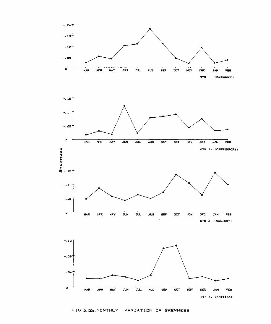
-.24

-.18

-.12

-.08

a MAR APR MAY JUN AUG SEP aCT NDV DEC .1AN FEe

8TN 1. (KASAR~~DI

-.15

-.1

-.OS

0 MAR APR MAY JUN J1JL AUK; SEP OCT NDV DEC .1AN FEe

10 8TN 2. (CANNANNOREI 11 (J

C ~ (J

J: ut -.15

-.1

-.05

0 MAR APR MAY JUN J1JL AUG SEP OCT NDV DEC .1AN FEe

~ 8TN 3. (CALICUTI

-.12

-.08

-.04

o MAR APR AUK; .1AN

8TN 4. (NATTIKAI

FIG .3.120. MONTHLY VARIATION OF SKEWNESS

best sorting with an average value of 0.82 ~. In August, the

sorting value is maximum (1.15 +) and the mean grain size 1S

coarsest (0.93 mm). This indicates that erosion" is active

till August. The samples are negatively skewed to nearly

symmetrical with most of the values clustered around -0.02,

-0.11 and -0.21 (Fig. 3.12a). However, during the rest of the

months, it is symmetrically skewed with values around -0.21.

The negative skewness indicates the erosional phase of the

beach from June to September while the symmetrical skewness,

the stable nature of the beach.

At Cannanore (Fig. 3.10a), the average mean S1ze of

the beach sand is 0.29 mm which belongs to medium grade sand

size. Coarsest size sand is observed in June (0.58 mm)

coinciding with high energy environment under the influence

of south-west monsoon. In August and October the sediments

shdws poorly sorting nature (Fig. 3.11a), while during the

rest of the year they are moderately well sorted to

moderately sorted. In general, throughout the period of

study, the sediments show a moderately sorted trend. The

skewness parameter (Fig. 3.12a), shows that during monsoon

months the sediment is negatively skewed while during the

rest of the period it was symmetrically skewed indicating an

erosion during June.

The beach at Calicut (Fig. 3.10a), is composed of

medium grade sand (0.26 mm to 0.40 mm) with moderate sorting

and symmetrical skewness except during October, November and

January, when coarse material is present. During January

71

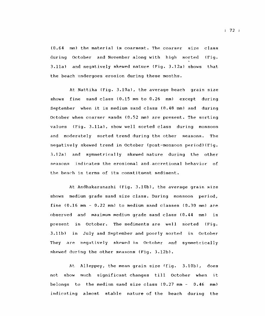
72

(0.64 mm) the material is coarsest. The coarser size class

during October and November along with high sorted (Fig.

3.11a) and negatively skewed nature (Fig. 3.12a) shows that

the beach undergoes erosion during these months.

At Nattika (Fig. 3.10a), the average beach grain size

shows fine sand class (0.15 mm to 0.26 mm) except during

September when it is medium sand class (0.48 mm) and during

october when coarser Rands (0.52 mm) are present. The sorting

values (Fig. 3.11a), show well sorted class during monsoon

and moderately sorted trend during the other seasons. The

negatively skewed trend in October (post-monsoon period)(Fig.

3.12a) and symmetrically skewed nature during the other

seasons indicates the erosional and.accretional behavior of

the beach in terms of its constituent sediment.

At Andhakaranazhi (Fig. 3.10b), the average grain size

shows medium grade sand size class. During monsoon period,

fine (0.16 mm - 0.22 mm) to medium sand classes (0.30 mm) are

observed and maximum medium grade sand class (0.44 mm) is I

present in October. The sediments are well sorted (Fig.

3.11b) in July and September and poorly sorted in October

They are negatively skewed J.n October and symmetrically

skewed during the other seasons (Fig. 3.12b).

At Alleppey, the mean grain size (fig. 3.10b), does

not show much significant changes till October when it

belongs to the medium sand size class (0.27 mm - 0.46 mm)

indicating almost stable nature of the beach during the

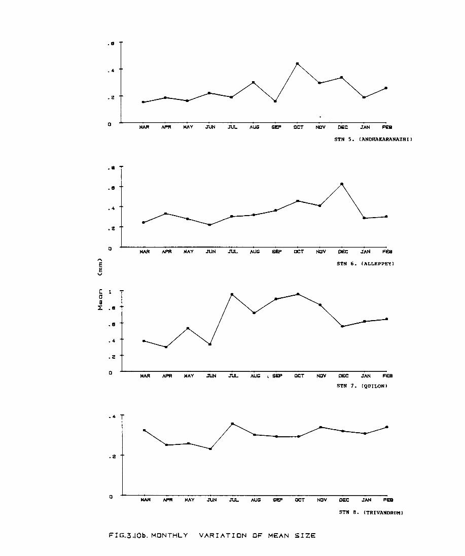
.8

.4

.2

a

STH 5. (AHDRAKARAHAZRII

.8

.8

.4

.2

a MAR N'R MAY J'UN JUL AUG SEP acT NQV DEC JAN FEB

" E STH 6. (ALLEPPEYI E v

C 1 0 ~ l: .8

.8

.4

.2

a MAR N'R MAY .ruN JUL AUG SEP acT NQV OBC .1AN FeB

8TH 7. (QOILOHI

.4

.2

a

8TN 8. (TRIVAHDROMI

F'I G.3 .IOb. MONTHLY VARIATION OF MEAN SIZE

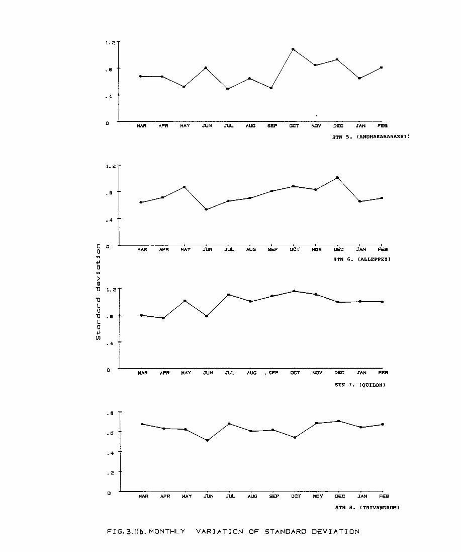
1.2

.8

.4

a MAR /\PR MAY AUG SEP aCT NDV DEC .rAN FEB

STN 5. (ANDHAKARANA1.HI)

1.2

.8

.4

MAA /\PR MAY .ruN .ruL AUG SEP aCT NaV DEC FEB C a a .... .... STN 6. (ALLBPPBY)

a .... > III "0 1.2

"0 l-a "0 .8 C a .... (J)

.4

a MAR '-\pR MAY .ruN .ruL. /lUG < SEP aCT NaV DEC .rAN FEB

STN 7. (QOILON)

.8

.6

.4

.2

a MAR /\PR MAY .ruL /lUG SEP aCT DEC .rAN FEB

STN 8. (TRIVANDROM)

FIG.3.lIb. MONTHLY VARIATION OF STANDARD DEVIATION

-.1

-.08

-.OB

-.04

-.02

o

8TN 5. (ANDHAKARANAZHI)

-.lS

-.1

-.05

D MAR APR "AY J'UN .JUt. AUG SE!" CCT NQV DEC 3AN FER

18 8TN 6. (ALLEPPEY) 18 (J

C ~ (J

.:s:: U) -.24

-.le

-.12

-. OB

0 MAR Al"R MAY J'UN .JUt. AUG SE!" acT NQV DEC 3AN FEB

8TN 7. (QUILON)

-.ca

-.04

-.02

o MAR APR IoIAY .1UN .1UL AUG SE!" OCT NQV DEC 3AN FEe

STN 8. (TRIVANDRUH)

FIG. 3.12b. MONTHLY VARIATION OF SKEWNESS

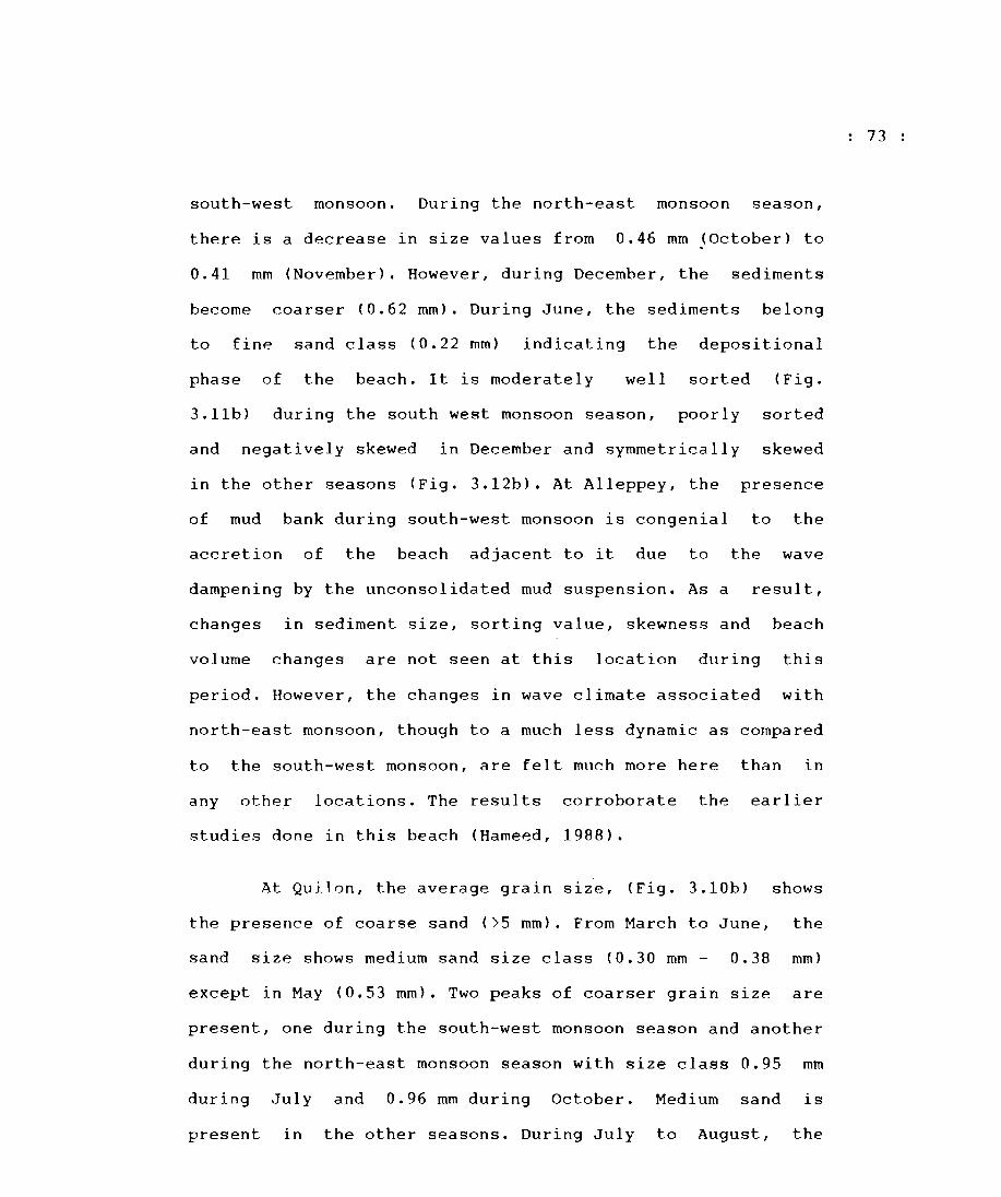
south-west monsoon. During the north-east monsoon season,

there is a decrease in size values from 0.46 mm (October) to

0.41 mm (November). However, during December, the sediments

become coarser (0.62 mm). During June, the sediments belong

to fine sand class (0.22 mm) indicating the depositional

phase of the beach. It is moderately well sorted (Fig.

3.11b) during the south west monsoon season, poorly sorted

and negatively skewed in December and symmetrically skewed

in the other seasons (Fig. 3.12b). At Alleppey, the presence

of mud bank during south-west monsoon is congenial to the

accretion of the beach adjacent to it due to the wave

dampening by the unconsolidated mud suspension. As a result,

changes in sediment size, sorting value, skewness and beach

volume changes are not seen at this location during this

period. However, the changes in wave climate associated with

north-east monsoon, though to a much less dynamic as compared

to the south-west monsoon, are felt much more here than in

any other locations. The results corroborate the earlier

studies done in this beach (Hameed, 1988).

At Quilon, the average grain size, (Fig. 3.10b) shows

the presence of coarse sand ()5 mm). From March to June, the

sand size shows medium sand size class (0.30 mm - 0.38 mm)

except in May (0.53 mm). Two peaks of coarser grain size are

present, one during the south-west monsoon season and another

during the north-east monsoon season with size class 0.95 mm

during July and 0.96 mm during October. Medium sand 1S

present in the other seasons. During July to August, the

73

sorting value shows a poorly sorted tendency (Fig. 3.11b).

The samples show negatively skewed nature (Fig. 3.12b) during

most of the period except during April and June when they are

symmetr.ical. This shows that the beach in general undergoes

erosion during the period of study.

At Trivandrum, the average value of the mean grain

size (Fig. 3.10b) shows the presence of' medium size sand

(0.25 mm - 0.36 mm) except in June where fine sand class is

present (0.23 mm). The maximum grain size in July shows the

severe erosion during this month. The sorting values (Fig.

3.11b) show moderately well sorted to moderately sorted

nature during south-west monsoon. And was symmetrically

skewed (Fig. 3.12b) through the .entire period of study

indicating the dynamically stable nature of the beach.

that

The

the

E.O.F analysis of the mean grain size data

first function accounted for 92.1% of the

shows

mean

square value while the second and third functions accounted

for 3.9% and 1.6% respectively (Table 3.2).

The first spatial eigen function (Ul) of the mean

grain size (Fig. 3.13) shows that, of all the beaches under

study, the beaches at Kasargod and Quilon have the highest

mean grain size whereas the beaches at Nattika and

Trivandrum have the least grain size values. In general, the

sediments are in the medium sand class except at Kasargod and

Quilon where they are coarse sized.

74

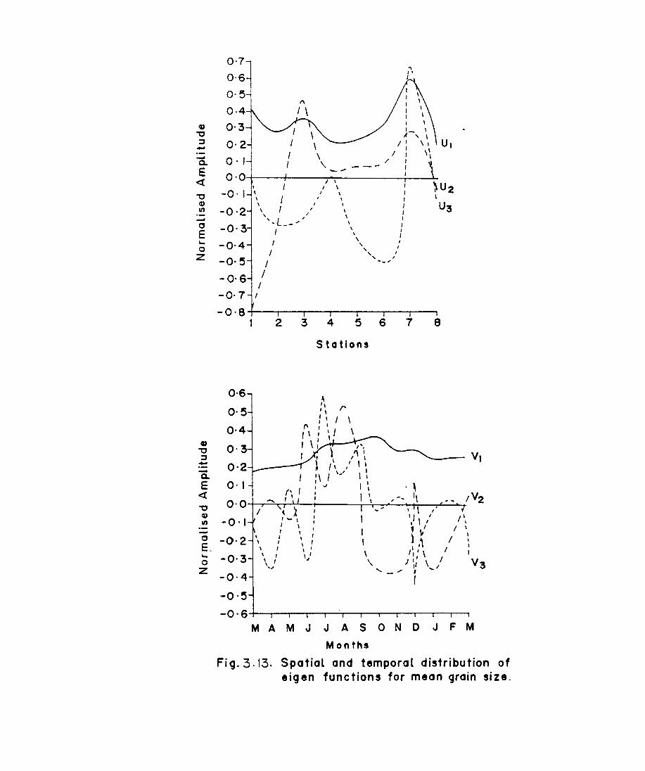
Q)

" ~ --Q..

E e:(

" q) en -0 E ... 0

Z

Q)

" ~ --Q..

E e:(

" Q)

en

0 E_ ... 0

Z

0·7 0·6

0'0 0-4 0·3

Ut

0·1 ,/ ----'" 0·0 I \ \ I I \ I ~U2 -0' I I I \ I

\ I \ I ,

\ I

, I U3 -0,2 , ,

\ I , , \

',L_-, I

" \ I -0,3 , , , I

I \ , -0,4 ,

.... I

I .... I

-0,5 .... I

I '- .. -0,6 I

I -0,7 I

-0,8 1 2 3 4 5 6 7 8

Stations

0·6 ~

0·5 " /" " : ' I \

0·4 (\ I I

,\ I ~ I

0·3 \ : ,'. \ ,'\ " VI I

0·2 I \ , , I,

I '-' I ~ :\ 0·' ,J I \ ' ,

r' , I I , .. -, " 0·0 ..... I ,

~ ,

/ ~ I , , , I I I -0,' ,- ,

I ' \ ' \ I

~ ..,' I \ , , , , , ~ ., /

, -0,2 \ , \

I • , , . I -0,3 \ , , ' \ I, • \ I

\ , J , ) .' I V3 , ,I \ / .J "- ", , "

-0,4 r -0,5

-0'64-~~---~~~~---~~~~---~

M A M J J A SON 0 J F M Mo n ths

Fi g. 3.\3. Spatial and temporal distribution of eigen functions for mean grain size.

The second spatial eigen function (U2) of the mean

grain size reflects the deviation in the grain size at a

given station from the mean. It also follows a similar trend

as that of the first eigen function indicating that the

maximum variability of the mean grain size is seen at

Kasargod and Quilon while at Nattika, Andhakaranazhi,

Alleppey and Trivandrum it shows least variability.

The corresponding temporal functions VI and V2 also

indicate a similar profile variations as discussed under

section 3.1.3. Since the third functions, both the spatial

and temporal, does not depict any beh~vioral pattern that can

be related to the physical phenomena, it has not been

considered for the present study.

75

CHAPTER 4

4. SEDIMENT TRANSPORT

4.1. Littoral Environmental Observations

The surf zone is of primary importance in forming

final pattern of sediment movement and thereby shaping

coasts. The Littoral Environmental Observation

the

the

(LEO)

programme provides data on wave period, breaker height, angle

of breaking waves to shoreline, breaking type, width of surf

zone and longshorp current speed and direction. The data

collection in this zone using gauges or other instruments is

difficult due to cost and inaccessibility. In the present

study, visual observations were carried'out once in a day,

for a period of one year at 8 selected stations using regular

measurement techniques.

4.1.1. Materials ~nd methods

Breaker wave characteristics

Heights of 10 consecutive breakers were estimated and

the average was noted as the significant wave height. The

wave period was measured using a stop watch by observing the

time required for 10 consecutive wave crests to pass a fixed

point and taking the average. The breaking wave angle with

respect to the coastline was measured using a surveyor's

magnetic compass. Most of the observations were made between

0600 & 0900 hrs irrespective of the tidal phase.

76

Longshore current

Longshore current velocity and direction were measured

by releasing neutrally buoyant floats in the surf zone and

the distance traveled by the floats in 2 minutes was recorded

and represented in m/so The measurement was repeated twice

and the average is noted. The approximate width of the surf

zone was visually estimated.

4.1.2. Results

Littoral Environmental characteristics

Monthly average variations of surf zone width, breaking

wave height, breaking period, breaking angle and longshore

current velocity and direction at stations 1 to 8 are

presented in (Figs. 4.1 to 4.8). Surfzone is seen to be wider

during the monsoon and post-monsoon seasons. It shows a

seasonal tendency in most of the study locations except at

stations 4 (Nattika) and at station 8 (Trivandrum). At

Nattika, the surf zone width is >10m during most of the time

irrespective of season due to gently sloping foreshore of

this beach. At Alleppey beach, the surf zone width is more

during the pre-monsoon period and post monsoon season than

during the monsoon season when it was <6m. The formation mud

bank during the south-west monsoon period of the year 1990,

(Joseph, 1992) provides calm conditions in the nearshore sea

and causes the low value of the surf zone width •

77

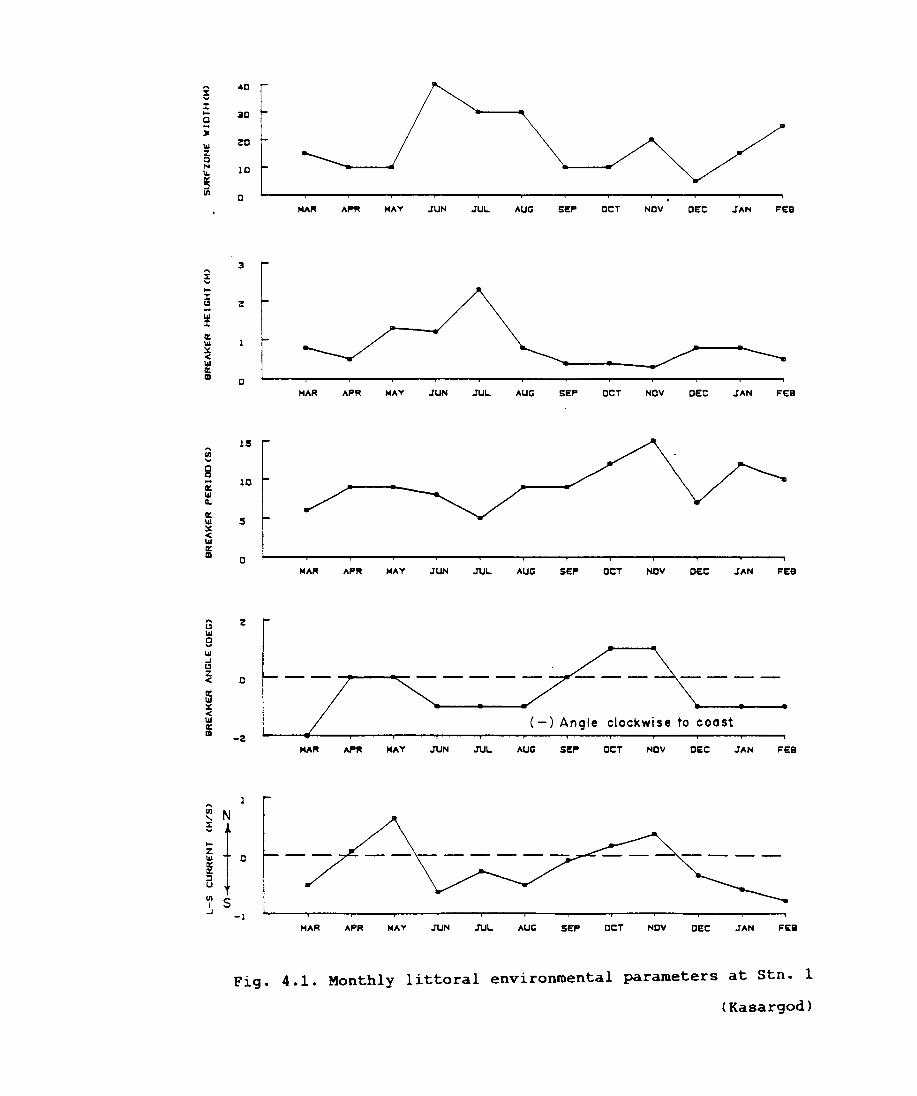
... 40 ::s:: '" x: .. 3D C .. :. III ZD Z Q ,..

lD '" a:: ::::J III

0

3 ... ! .. x: Cl Z .. III x: a:: III X < III a:: ID

0

lS ... ~ C Q ... 10 a:: III Go

a:: 5 III

X < III a:: ID 0

a 2 III e III

G z <

ffi X < III a:: ID

... III "-::s:: '" .. Z III a:: a:: ::::J u III I

.J

o

-2

N

f 0

S -1

MAR A~R MAV .lUN

MAR ~R MAY .lUN

MAR APR MAY J'UN

APR MAY .lUN

MAR APR MAV .lUN

.lUL. AUG SEP OCT NDV OEC .lAN FEB

.lUL. AUG SEP DCT NDV OEC .lAN FEB

J'UL. AUG SEP OCT NDV DEC .lAN FEB

(-) Angle clockwise to coast

J'UL. AUG SEP OCT NOV DEC .lAN FEB

J'UL. AUG SEP OCT NDV OEC .lAN FEB

Fig. 4.1. Monthly littoral environmental parameters at stn. 1

(Kasargod)

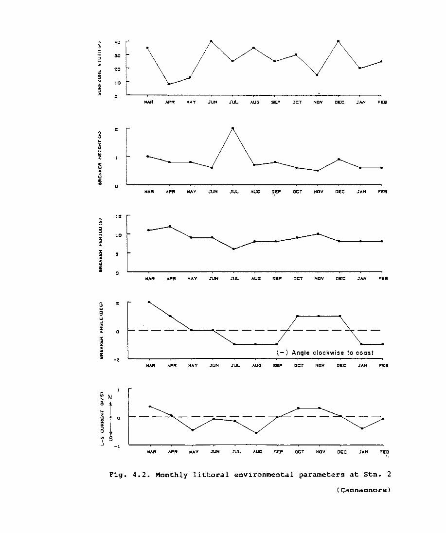
! 40

l: ... 3D C ... :. III za z a ~ 10 11: ::J 1/1

0 MAR APR MAY JUN JUL AUG SEP aCT NOV OEC JAN FEa

z '"' ! ... l: 12 ... III l:

11: III le < III 11: III

0 MAR APR MAY JUN JUL AUG SEP aCT NOV O£C JAN FlEa

"

IS '"' !!! c a ... la 11: III 11.

11: 5 III

le

~ 11: III a

MAR ~ MAY JUN JUL AUG SEP aCT Nav DEC JAN FlEa

- - - -----'-.-- -- -- ----

(-) Angle clockwise to coast

MAR MAY JUN AUG SEP aCT Nav OEC JAN FEa

'"' III N "-s

f .., ... Z III 0 11: 11: ::J U

III S I ..J -1

MAR APR MAY JUN JUL AUG SIEP aCT Nav D£C JAN FlEa "

Fig. 4.2. Monthly littoral environmental parameters at stn. 2

(Cannannore)

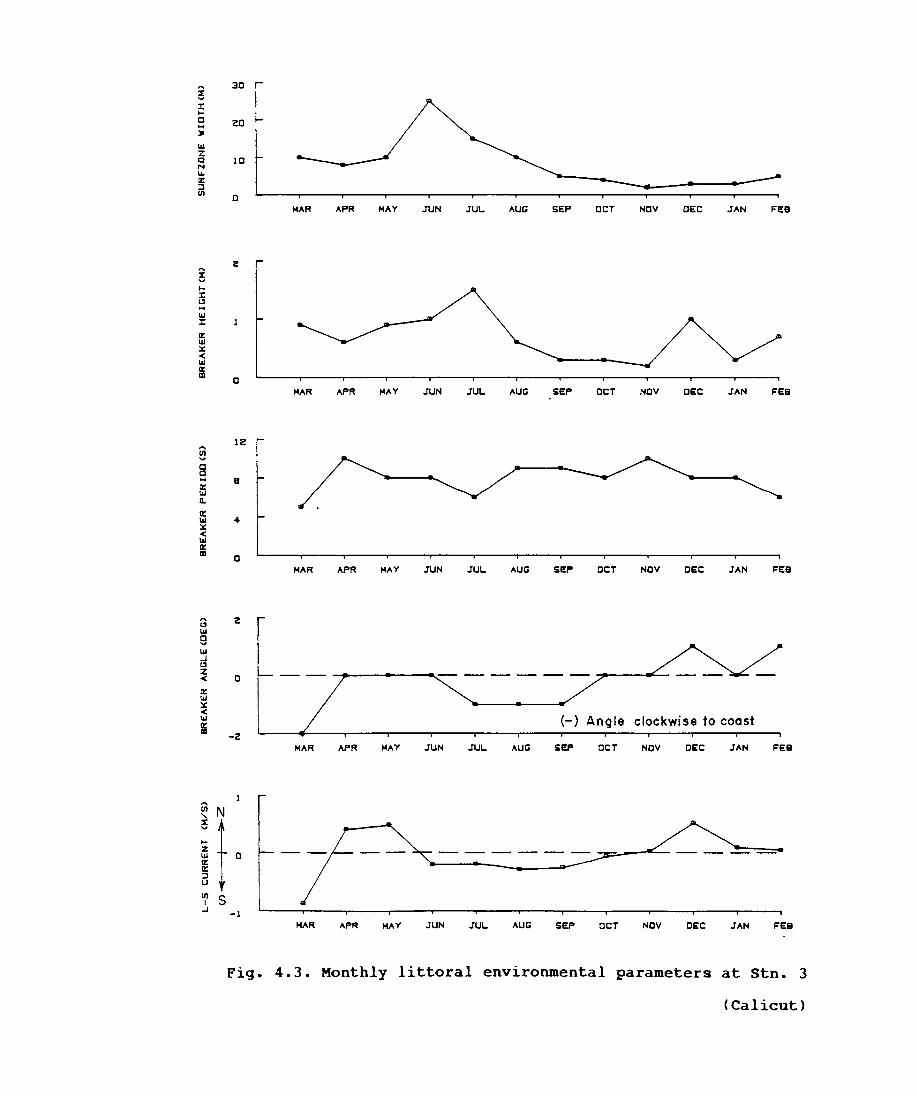
" 3D ~ X l-Q 20 ... :JI

1&1 Z Q ID .... I&. It: ::::I 1/1 0

MAR APR MAY JUN JUL AUG SEP OCT NOY OEC JAN FEB

2 '" X ... l-X Cl ... 1&1 X

It: 1&1 X < 1&1 It: III

0 MAR APR MAY JUN JUL AUG SEP OCT NOY OEC JAN FEB

12 " 1/1 ... Q Q ... 15

8

11.

It: 1&1 4 X < 1&1 It: III 0

MAR APR MAY JUN JUL AUG SEP OCT NOY OEC JAN FEB

'" 2 Cl 1&1 Q ... 1&1 ..J Cl Z < 0

It: 1&1 X <

(-) 1&1 Angle clockwise to coast It: ID -2

MAR APR MAY JUN JUL AUG SEP OCT NOY DEC JAN FEB

" 1/1 N " ~

t I-Z ------1&1 a It: It: ::::I u 1/1 5 I .J -1

MAR APR MAY JUN JUL AUG SEP aCT NOY DEC JAN FEB

Fig. 4.3. Monthly littoral environmental parameters at stn. 3

(Calicut)

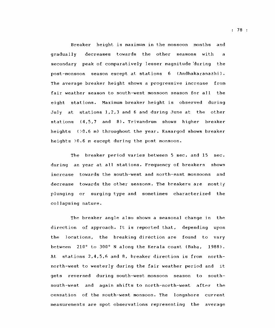
Breaker height is maximum in the monsoon months and

gradually decreases towards the other seasons with a

secondary peak of comparatively lesser magnitude auring the

post-monsoon season except at stations 6 (Andhakaranazhi).

The average breaker height shows a progressive increase from

fair weather season to south-west monsoon season for all the

eight stations. Maximum breaker height is observed during

July at stations 1,2,3 and 6 and during June at the other

stations (4,5,7 and 8). Trivandrum shows higher breaker

heights (>0.6 m) throughout the year. Kasargod shows breaker

heights >0.6 m except during the post monsoon.

The breaker period varies between 5 sec. and 15 sec.

during an year at all stations. Frequency of breakers shows

increase towards the south-west and north-east monsoons and

decrease towards the other seasons. The breakers are mostly

plunging or surging type and sometimes characterized the

collapsing nature.

The breaker angle also shows a seasonal change in the

direction of approach. It is reported that, depending upon

the locations, the breaking dir~cti6n are found to vary

between 210 0 to 300 0 N along the Kerala coast (Baba, 1988).

At stations 2,4,5,6 and 8, breaker direction is from north­

north-west to westerly during the fair weather period and it

gets reversed during south-west monsoon season to south­

south-west and again shifts to north-north-west after the

cessation of the south-west monsoon. The longshore current

measurements are spot observations representing the average

78

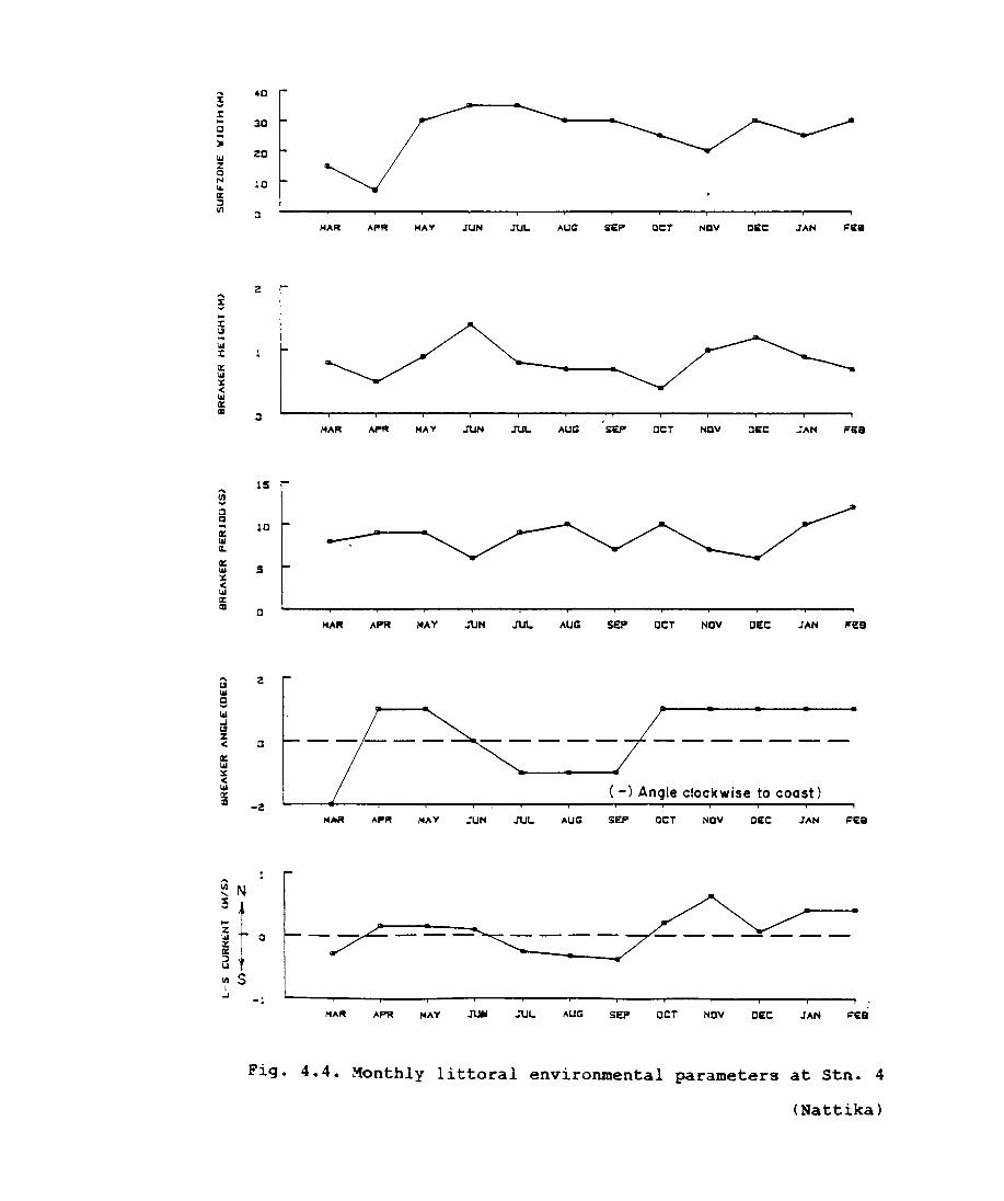
g 40

~ ... la 0 .. :Jo

IM 2:0 z a ,...

10 l&. lE ::J III a

2: " ! ... ~ (.:I .. IM ~

lE IM :s: < IM lE III a

" 15

~ 0 a .. 10 lE IM a. lE

! IM :s: < IM lE III

0

a 2: IM 9 IM a z <

15 :s: < IM lE III

" ~ N

a

-2

~ a : t ~ u III S I

..J -1

MAR AP" MAY

MAR "'"Ill MAY

HAR AfOR HAY

MAY

MAR "PR HAY

.1UN .1UL. AUG SEP OCT Nay OEC .1AN FEll

.ruN .1UL. AUG SEP aCT Nay aEC .1AN FE.

.1UN .1UL AUG SEP aCT NOV CEe 1AN FEB

( -) Angle clockwise to coast)

.1UN AUG SEP aCT Nay eEC 1AN FE.

.1UL AUG SEP OCT NOV eEe 1AN FEB

Fig. 4.4. Monthly littoral environmental parameters at Stn. 4

(Nattika)

i ~

1: ... C ... :JI

1&1 z a ,.. "" a: :J UI

.... ! I-1:

'" ... 1&1 1:

a: 1&1 x < 1&1 a: III

.... UI ~

C a ... a: 1&1 IL

Qi: 1&1 X < 1&1 Qi: III

.... UI .... ! ... Z 1&1 Qi: Qi: :J U

UI I

.J

4D

3D

2a

ID

a MA" AP" MAY JUN JUl.. AUG SEP aCT Nav OEC JAN FEB

2

a MA" AP~ MAY JUN JUL AUG SEP OCT Nav OtiC JAN FEB

IS

la

5

a MAR APR MAY JUN JUL AUG SEI- aCT NQV OEC JAN FtiB

(-) Angle clockwise to coast

MAR APR MAY JUN JUL AUG SEP aCT Nav OEC JAN FEB

N

t a

S -1

MA" APR MAY JUN JUL AUG SEP aCT Nav OEC JAN FEB

Fig. 4.5. Monthly littoral environmental parameters at stn. 5

(Andhakaranazhi)

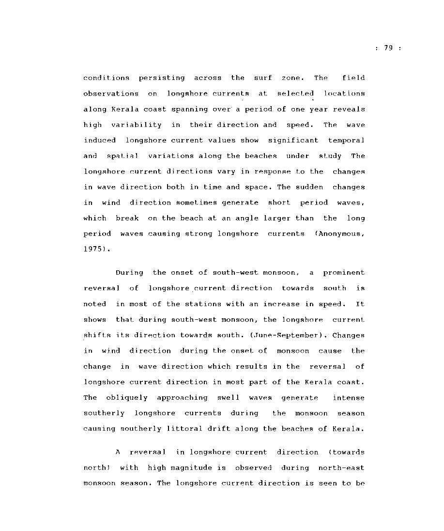
conditions persisting across the surf zone. The field

observations on longshore currents at selected locations

along Kerala coast spanning over a period of one year reveals

high variability in their direction and speed. The wave

induced longshore current values show significant temporal

and spatial variations along the beaches under study The

longshore current directions vary in response to the changes

in wave direction both in time and space. The sudden changes

in wind direction sometimes generate short period waves,

which break on the beach at an angle larger than the long

period waves causing strong longshore currents (Anonymous,

1975).

During the onset of south-west monsoon, a prominent

reversal of longshore.current direction towards south is

noted in most of the stations with an increase in speed. It

shows that during south-west monsoon, the longshore current

shifts its direction towards south. (June-September). Changes

in wind direction during the onset of monsoon cause the

change in wave direction which results in the reversal of

longshore current direction in most part of the Kerala coast.

The obliquely approaching swell waves generate intense

southerly longshore currents during the monsoon season

causing southerly littoral drift along the beaches of Kerala.

A reversal in longshore current direction (towards

north) with high magnitude is observed during north-east

monsoon season. The longshore current direction is seen to be

79

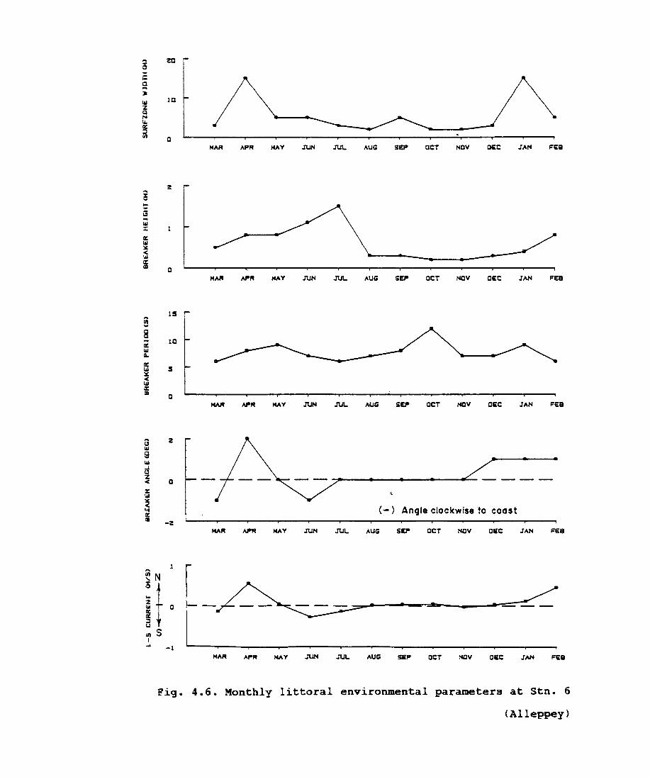
.... za ! :: ... a .. :. 111 la z Cl N I&. QC :J III a

MAR -'PR MAY J'UN J'UL AUG SIEP' aCT NaY IJEC ~AN FEll

z .... s: .., ... :: Cl .. 111 :: QC 111 X < 111 ac all a

MAR Al"'R MAY J'UN JUL AUG SEP aCT Nay IJEC ~AN FEll

IS .... 1/1 ..,

El .. la ac 111 Ii.

ac 5 111

X < 111

i a MAR Al"'R MAY J'UN J'UL AUG SIEP' aCT NaY IJEC ~AH FEll

(-) Angle clockwise to coast

MAY J'UN J'UL AUG aCT Nay IJEC ~AN FEll

MAR MAY J'UN JUL AUG SEP aCT Nay IJEC ~AH FEll

Pig. 4.6. Monthly littoral environmental parameters at stn. 6

(Alleppey)

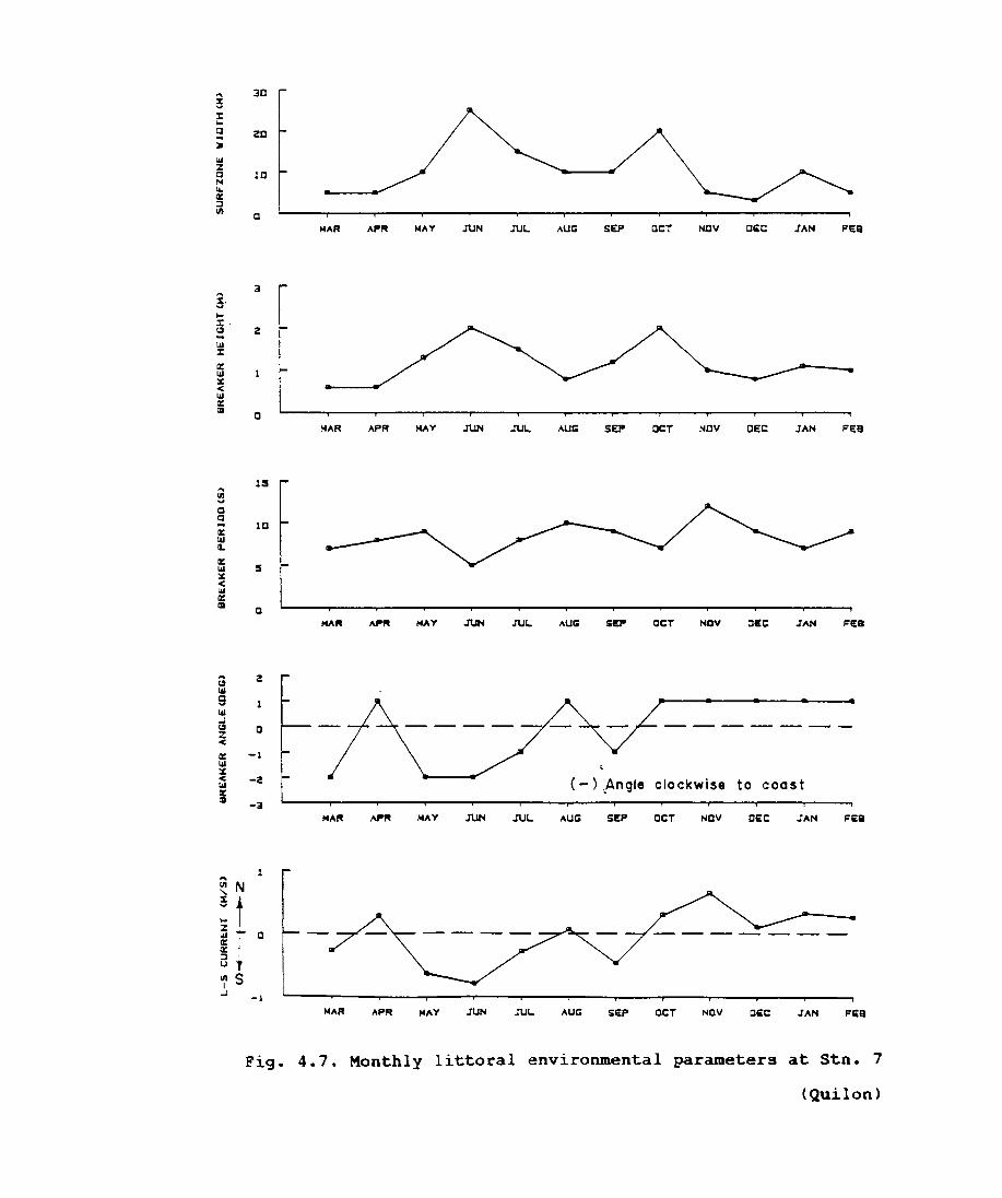
" ! : l-Q ... :. III Z Q ,... l&. GI: :l UI

" % . .... I-l:. t.:I ... III l:

GI: III X < III GI: III

... UI .... Q Q ... GI: III IL

GI: III X < III GI: III

... t.:I III e III .J t.:I z < GI: III X < III GI: III

... UI "-% .... I-Z III GI: GI: :l U

UI I

.J

3D

2D

IQ

a MAR APR MAY JUN JUL AUG SEP aCT NQV ali:c JAN FEB

3

2

a MAR APR MAY JUN JUL AUG sa- aCT NQV CEC JAN FEB

us

IQ

5

a MA" AI"" MAY JUH JUL AUG sm- aCT NaV acc JAN F£B

2

a

-1

-2 (-) .Angle clockwise to coast -3

MAR MAY JUN JUL AUG SE'"' aCT NQV OEC JAN FIi:B

N

t a

5 -1

MAR APR MAY JUN JUL AUG SEP aCT NQV OEC JAN FIi:B

Fig. 4.7. Monthly littoral environmental parameters at Stn. 7

<Quilon)

... ! l: ... 0 ... » UI Z 0 N lI. Il!: ~ lA

... 3' ... l: I.!I ... UI l:

Il!: UI X < UI Il!: 121

... lA .... 8 ... Il!: UI A-

Il!: UI x < UI Il!: 121

.... t2 UI 0 .... UI ~ I.!I Z < Il!: UI X < UI Il!: 121

40

30

20

10

a HAR APR HAY JUN JUI.. AUC; SEP aCT NOV a;:c JAN FEB

:3

2

a HAR APR HAY JUN JUI.. AUC; SE!'" aCT NOV DEC JAN FEB

15

10

5

a HAR APR HAY JUN JUI.. AUG SI!P aCT NOV a;:c JAN FEB

2

a ---- ..... --.....

(-) Angle clockwise to coast -2

HAR APR HAY JUN JUI.. AUG SEP aCT NCV DEe JAN FEB

APR HAY JUN JUI.. AUG SEP aCT NOV alc JAN FEB

Fig. 4.8. Monthly littoral environmental parameters at stn. 8

(Trivandrum)

transitional and inconsistent during March, December and

January. A progressive increase in current velocity occurs

from November through January and February along the studied

locations. Current speed upto 0.88 m/sec is observed in the

Trivandrum beach during November, which is highest among the

recorded values on the beaches studied along the Kerala coast

during this period. Current speeds of 0.2 - 0.6 m/sec. are

frequently recorded at many locations. Negligible current

velocity (0.02 to 0.05 m/sec.) values are also recorded at

stations 3 and 6, ie. at Calicut and Alleppey,

during the period of study.

frequently

4.2. Longshore sediment transport

The longshore movement of beach sand poses a potential

littoral problem. The important factor governing the beach

erosion is the longshore sediment transport which is

controlled predominantly by waves and nearshore" topography.

An understanding of sediment transport on beaches 1S also

necessary for the analysis of formation of the geomorphic

features such as sand spits and barrier islands, to examine

the tidal inlet processes and to understand the

irregularities in the shoreline. Interruptions of these

natural movements of sands by man made barriers like groins,

breakwaters, jetties etc. result in sediment

the updrift side and removal of sediments on

deposition on

the downdrift

side. This results in the necessity to study the longshore

sediment transport around inshore coastal areas, which is of

80

fundamental inlerest to coastal engineers in the planning of

structures, dredging activities of ports and spoil disposal.

A proper understanding of the seasonal littorai transport

trend lS important for the efficient management and

development of coasts. Beach erosion problems along this

coast have been the initial motivation for this study on sand

transport by estimating the rate of sand movement.

Since estimation of the rate of littoral sand drift is

one of the essential items necessary for the field

investigation in regard to beach protection and sedimentation

problems, much effort has been made in establishing a method

of estimation by coastal engineers for a long time. The

dynamics of sediment mov~ment in the littoral zone lS

governed primarily by the wave induced currents. Specific

knowledge of these currents and associated circulation

patterns are helpful in better utilization of the coastal

environment.

In the nearshore area, waves arriving from offshore

continuously bring in momentum, energy and mass. Since the

shoreline provides a fixed boundary, the momentum and energy

fluxes are dissipated in the surfzone. Most of the energy is

converted to turbulence in the breaker zone but enough is

left to drive a nearshore current system and move loose bed

material. The momentum brought in by the waves will drive the

littoral current system and cause a local set-up or set-down

of the mean water level.

81

The dynamics of sediment movement in the littoral zone

depends mainly on four factors: the nature of the material

available for transport, orientation and other "geomorphic

features of the shore, the angle of wave approach and the

wave induced currents. Waves arriving at the shore are the

primary cause of sediment transport in the littoral zone.

Higher waves break further offshore, widening the surfzone

and setting more sand in motion. Changes in wave period or

height result in moving sands onshore or offshore. The

knowledge about the wave climate - the combined distribution

of wave height, period and direction during different seasons

is required for an adequate understanding of movement of

sand in any specific area. The cellular circulation patterns

in the surf zone depend on the longshore gradient in wave set­

up. Because of the turbulence due to breaking and surging of

waves, large volumes of sediments are placed in suspension or

rolled along the bed in the surfzone.

4.2.1. Materials and methods

There have been many investigatiohs in the littoral

zone for the quantitative and qualitative estimation of

sediment drift, making use of the relationship between wave

forces and transport of sediment. Many studie~ have been

carried out on the theoretical estimation of the longshore

sediment transport using laboratory and field experiments.

Longshore sediment transport is generally estimated by uSlng

empirical equations which relate the longshore energy flux in

82

the breaker zone to the longshore transport rate. (Graff and

Overeem, 1979; Willis, 1980). Empirical equations, using

results of the wave refraction studies and progressive

changes in grain size distribution have also been used to

indicate sediment transport direction. Some analyses are more

sophisticated by taking into account the frictional factors

and bed permeability_ These also assume for convenience, a

constant mean sediment size. It has been shown later that

these assumptions were far from reality during the short

periods when the bulk of the littoral drift takesplace.

Komar (1976) presented graphically, various data

indi6ating relationships between the longshore transport rate

and

Inman

the longshore component of wave energy flux.

(1970) made extensive field measurements and

Komar and

an approach of longshore transport with the immersed

proposed

weight

of longshore transport of sand proportional to the longshore

component of wave energy flux. Shore Protection Manual

(Anonymous, 1975), presents different equations for

estimating the longshore transport using the relationship

between longshore energy flux factor (PIs) and the longsqore

transport rate (Q).

Almost all studies have attempted to relate, the

longshore sediment transport with longshore energy flux in

the form,

Q = K. PIs ( 4 . 1 )

where Q = volume rate of longshore sediment transport.

K - dimensional constant

83

PIs = longshore component of wave power at breaking

= P cos cC b sin cC b where

P = wave power at breaking = ( E Cn)b

oC b = breaking angle

E = wave energy

Cn = group celerity and suffix b denotes at breaker zone

Using the value of PIs in equn. (4.1)

( 4 • 2 )

Walton (1980) established a computing technique for

longshore energy flux factor (PIs) using the longshore

current and breaking wave height.

By radiation stress principle, the longshore current is given

by the relation ( Longuet-Higgins, 1970)

5 /8 (k / ( d )0.5"" oC Vb = - nap Cf) g b m S1nOC b cos b ( 4 • 3 )

where

Vb = longshore current velocity at breaker zone

p = a mixing parameter

db = breaking depth

ef = bottom friction factor

In = beach slope

Ra = breaking wave amplitude/water depth

Using the relationship (2Ra = Hb/db) in equn. (4.3)

Vb = 5 n/16 ka p/ Cf (1/2ka )0.5 m (9db)0.5 sin 2~b (4.4)

The longshore current velocity at any point in the surf zone

can be defined as

( 4 • 5 )

where

84

v = longshore current velocity within the surf zone

Vo = theoretical Longshore current velocity at breaking

(no mixing)

using ( 4 • 3 ) and ( 4 • 4 )

V = (V/VO)(5TT/16)(ka /Cf)(1/2 ka )0.5 m (9d b)0.5 sin 2ltb ( 4 .6)

The relationship for longshore energy flux factor at surface

is given by

PIs = (4.7)

For breaking zone, substituting Cb = (g db)0.5 in equn. (4.8)

PIs = r Bb2 / 16 (db/Bb)0.5 (g Bb)0.5 sin 20Cb ( 4 • 9 )

Using equn. ( 4.7) and assuming m = db/ W

P Bb W V Cf --------------------PIs = (4.10) 0.78 ( 5 TI/2) (V/Vo )

Equn. (4.1) become

Q = K PIs

ie Q = K (' g Bb W V Cf (4.11)

0.78 (5 TT/2) (V/Vo )

where Q is the annual longahore sediment transport

rate in

constant.

r =

9 =

3 m /yr and the value K =

1025 kg/m 3

2 9.81 m/a

1288 is a dimensional

ef = 0.01 = frictional coefficient dependent on bottom

excursion and bottom roughness.

Bb = breaking wave height in m

W = surf zone width in m

V = longshore current velocity

85

v theoretical dimensionless longshore current =

Vo velocity, (Longuet-Higgins, 1970), assumed

mixing parameter p = 0.4 and is dependent on the

parameter X/Wo

For the estimation of sediment transport rate using

the daily data of LEO, only Walton's equation can be well

suited, as it takes into consideration the measured values of

longshore current. Chandramohan et al. (1993) have used this

equation for the estimation of longshore sediment transport

along the south Maharashtra coast. The primary concern for

such studies 1S to make estimations on breaker height,

breaker period and longshore current direction and speed.

Monthly averages of the daily LEO data for one year made at

each station have been used in equation (4.11). The net

transport (difference between the amount of littoral drift

transported to the north and south across the surf zone for a

given period) has been calculated.

4.2.2. Results

Monthly longshore sediment transport

estimated using Walton's equation (4.11) from

rates were

the littoral

environmental parameters on breaker height, surfzone width

and longshore current direction and speed at all 8 stations.

(Figs. 4.9 to 4.16 and Table. 4.1). The negative sign in the

table indicate the drift towards south and the positive sign

towards north. Annual net transport for each location is

presented in Fig. 4.17.

86

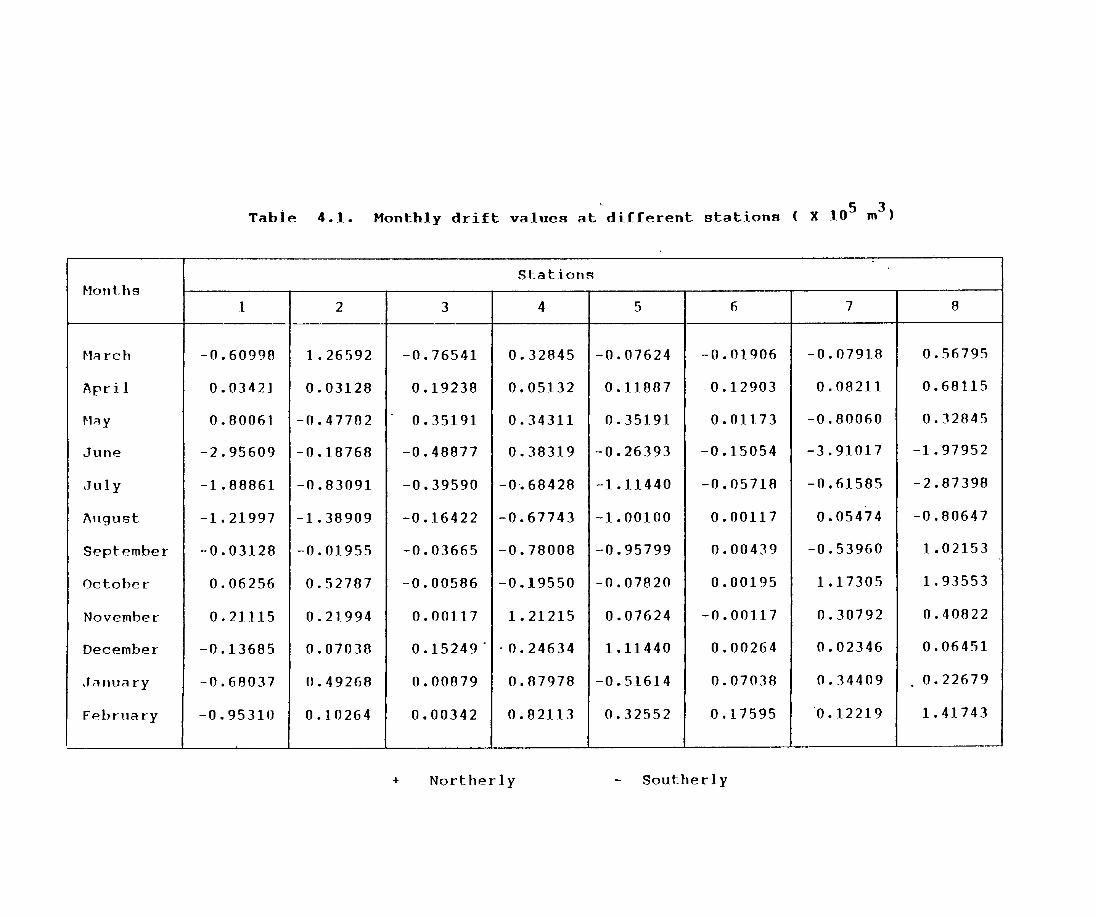
Tabie 4.1. Monthly drift values at different stations ( X 105 m3 )

StationR Hont.hs

1 2 3 4 5 6 7 8

~1a rch -0.60998 1. 26592 -0.76541 0.32845 -0.07624 -0.01906 -0.07918 0.56795

April 0.03421 0.03128 0.19238 0.05132 0.11807 0.12903 0.08211 0.68115

~1ay 0.80061 -0.47782 0.35191 0.34311 0.35191 0.01173 -0.80060 0.32845

June -2.95609 -0.18768 -0.48877 0.38319 -0.26393 -0.15054 -3.91017 -1.97952

,July -1.88861 -0.83091 -0.39590 -0'.68428 -1.11440 -0.05718 -0.61585 -2.87398

August -1.21997 -1.38909 -0.16422 -0.67743 -1.00100 0.00117 0.05474 -0.80647

September -0.03128 -0.01955 -0.03665 -0.78000 -0.95799 0.00439 -0.53960 1.02153

october 0.06256 0.52787 -0.00586 -0.19550 -0.07820 0.00195 1.17305 1. 93553

November 0.21115 0.21994 0.00117 1.21215 0.07624 -0.00117 0.30792 0.40822

December -0.13685 0.07030 0.15249" " 0.24634 1.11440 0.00264 0.02346 0.06451

.J a JlUil ry -0.68037 0.49268 0.00879 0.07978 -0.51614 0.07038 0.34409 ,0.22679

February -0.95310 0.10264 0.00342 0.82113 0.32552 0.17595 0.12219 1. 41743

---- --- --- -- --- ---

+ Northerly Southerly

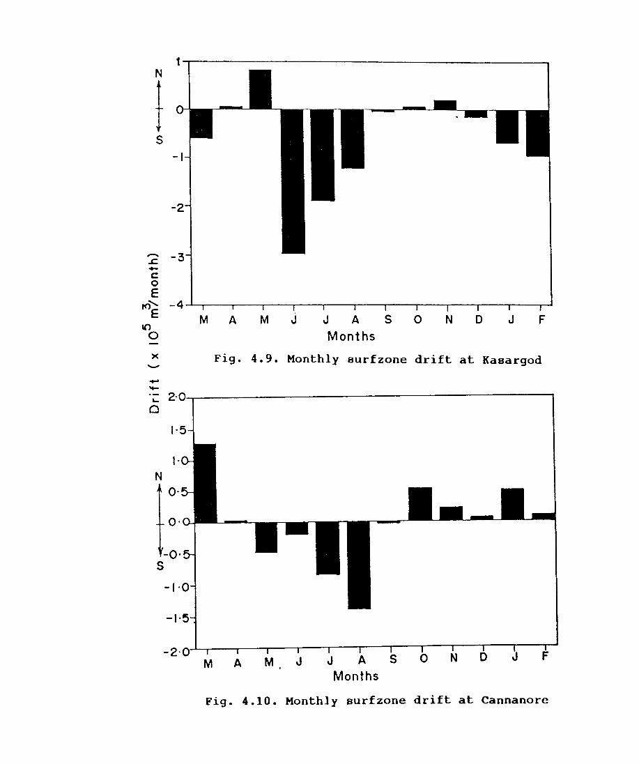
N

f s

-.c -c 0 E

tt>' E -4

10 0

)(

'-'

.... .... L.. 2·

0

1·5

I· N

O·

o·

-0' S

-1,0

-1,5

-2'

M A

Months

Fig. 4.9. Monthly aurfzone drift at Kaaargod

J Months

Fig. 4.10. Monthly aurfzone drift at Cannanorc

Along Kasargod beach (Fig. 4.9), the littoral drift

shows higher values compared to all other beaches. In the

pre-monsoon season southerly drift is observed"during March

and northerly drift during April-May. During May, the drift

magnitude amounts to 0.8 X 10 5 m3 • with the onset of south-

west monsoon, a shift to southerly direction is observed in

June and continues in the same direction till the end of

south-weRt monsoon. Maximum southerly drift is observed 1n

June (2.95 X 10 5 m3 ). During post-monsoon season, the drift

is low and inconsistent in direction. During January to March

the drift is southerly. The annual net transport shows a

southerly drift of 0.73 X 10 6 3 m which is the highest

compared to the other locations. The higher drift magnitude

along this beach is due to the' high energy conditions

prevailing along this beach. (Chapter 4, Section 4.1.2).

Along Cannanore section (Fig. 4.10), it is seen that,

during pre-monsoon period the drift is northerly with a

maximum value of 1.26 X 10 5 m3 in March. The beach showR

southerly littoral drift during May - September and it is

northerly during the other months. A decrease in magnitude is

observed during June (0.19 X 105 m3 ) followed by an increas0

5 3 towardR AllgUSt (1.38 X 10 m). From September onwards the

drift is consistently directed towards north. The annual net

drift is southerly with a magnitude of 0.019 X 10 6 m3 •

Along the Calicut beach (Fig. 4.11), the littoral

drift values show lesser magnitude compared to the locations

on the north. The monthly drift is southerly during March

87

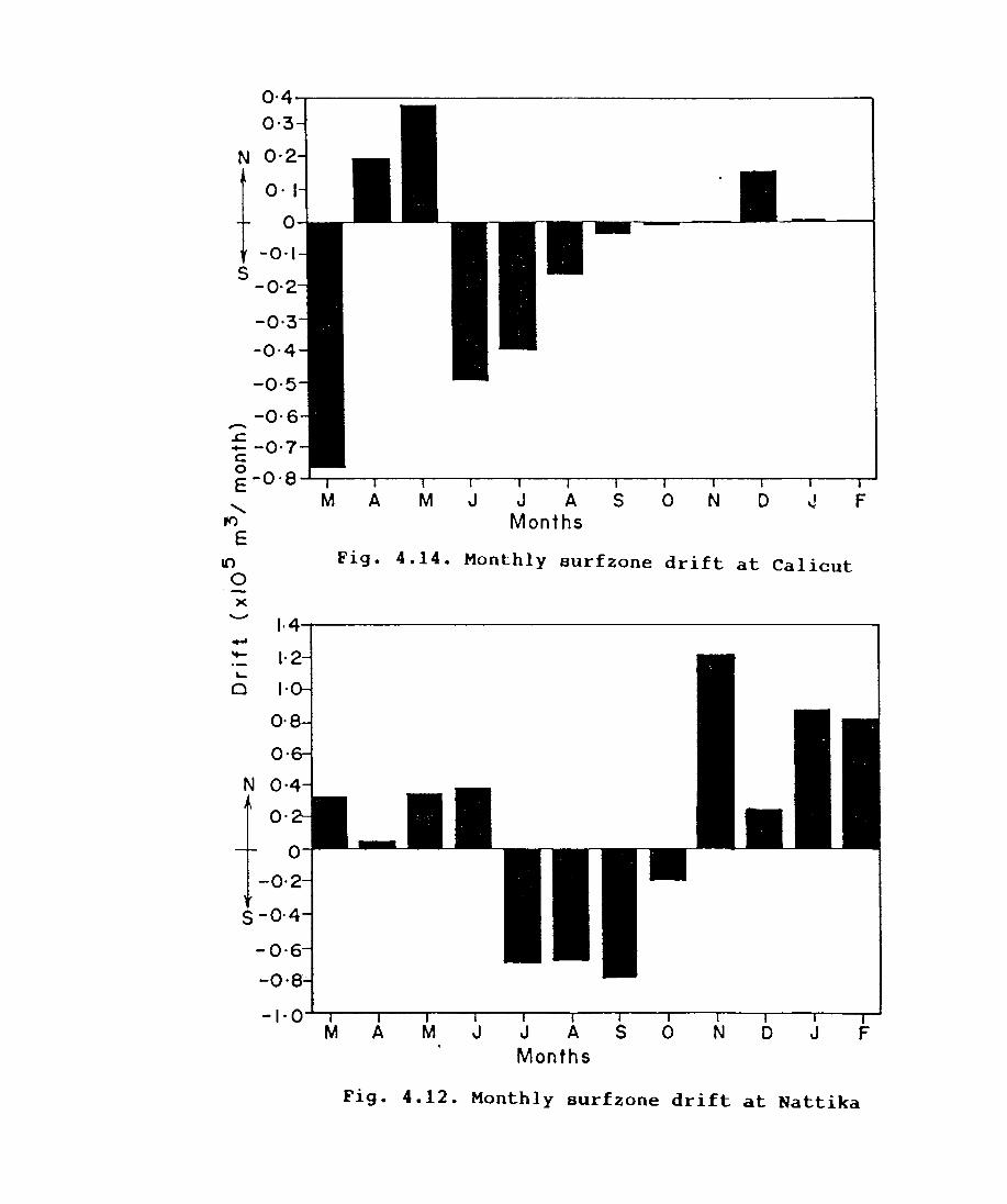
0'4~--------------------------------------, 0·3

N 0·2

0·1

-

" ft')

E 10

0 -x .........

I· ... ..... I· ~

Q I·

O·

o· N o·

o·

-0'

-0'

M A M J J A S o N Months

Fig. 4.14. Monthly Burfzone drift at Calicut

-I'O~~~---'--'---Jr--.---r--.---r--'--~--II

Months

Fig. 4.12. Monthly surfzone drift at Nattika

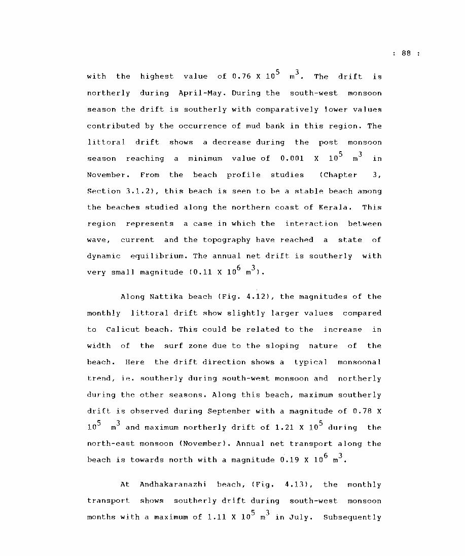
with the highest value 5 of 0.76 X 10 3 m • The drift is

northerly during April-May. During the south-west monsoon

season the drift is southerly with comparatively lower values

contributed by the occurrence of mud bank in this region. The

littoral drift shows a decrease during the post monsoon

season reaching a minimum value of 0.001 X 10 5 m3 in

November. From the beach profile studies (Chapter 3,

Section 3.1.2), this beach is seen to be a stable beach among

the beaches studied along the northern coast of Kerala. This

region represents a case in which the interaction between

wave, current and the topography have reached a state of

dynamic equilibrium. The annual net drift is southerly with

very small magnitude (0.11 X 106 m3 ).

Along Nattika beach (Fig. 4.12), the magnitudes of the

monthly littoral drift show slightly larger values compared

to Calicut beach. This could be related to the increase in

width of the surf zone due to the sloping nature of the

beach. Here the drift direction shows a typical monsoonal

trend, le. southerly during south-west monsoon and northerly

during the other seasons. Along this beach, maximum southerly

drift is observed during September with a magnitude of 0.78 X

105 m3 and maximum northerly drift of 1.21 X 105 during the

north-east monsoon (November). Annual net transport along the

beach is towards north with a magnitude d.19 X 106 m3 •

At Andhakaranazhi beach, (Fig. 4.13), the monthly

transport shows southerly drift during south-west monsoon

months with a maximum of 1.11 X 10 5 m3 in July. Subsequently

88

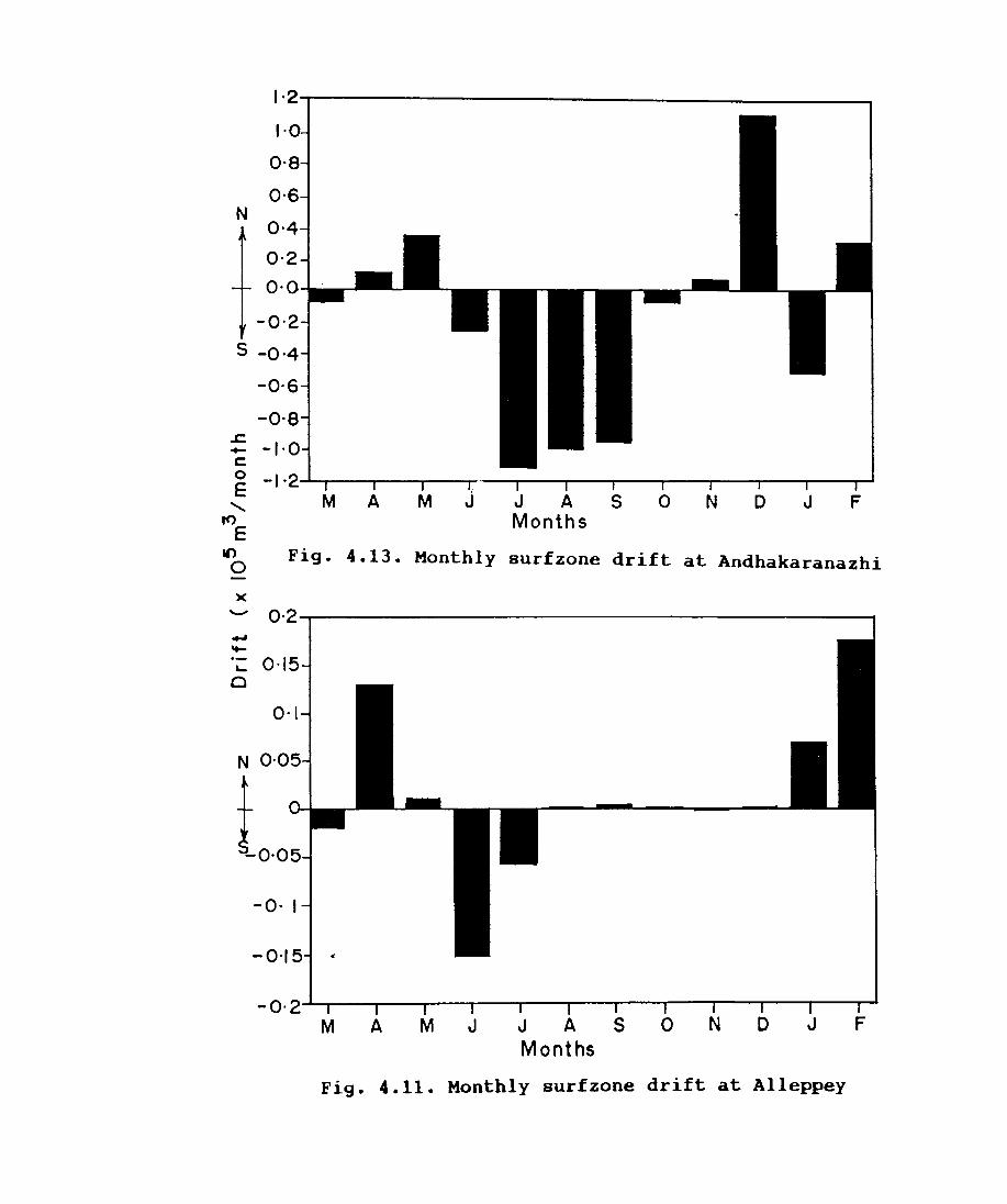
1'2~------------------------------__________ ~

N o·

-0,2

S -0,4

-0'6

-0'8

== -1,0 c E -I ·2...L.....,...-----,--'T----r

" rt')

E ~ Fig. 4.13. Monthly surf zone drift at Andhakaranazhi o

)(

~ 0·2--------------------------------------------------------------------. ~ It-

'- 0-15 ca

0-1

N 0-0

1000 -0' I

-0-15

"';0-2

4

M A M J J A Months

F - 4 11 Monthly surfzone drift at Alleppey ~g. • •

the magnitude decreases towards October. In all the other

months except March and January the drift 1S seen towards

north. Another peak value of the drift towards north is

observp.d during the north-east monsoon season (December).

Results of the earlier investigations showed similar features

in this region. (Prasannakumar, 1985). The annual net drift

along this stretch of the beach is southerly with magnitude

of 0.2 X 106 m3 •

Monthly drift values estimated for the Alleppey beach

(Fig. 4.14), show southerly drift with low magnitudes during

south-west monsoon season. These low values may be due to the

occurrence of the mud bank off this location which brings out

calm conditions in this region. In.all other months except

March, the drift is northerly. A maximum northerly drift of

0.13 X 10 5 m3 occurs in April and is followed by a reversal

1n direction towards south in the beginning of south-west

monsoon season. The drift values are negligible during August

to December «0.005 X 10 5 m3 /month). The annual net drift

value shows a northerly drift (0.016 X 106 m3 ) which is least

compared to the other beaches examined~ The beach profiles

(Chapter 3, Section. 3.1.2), also show the stable nature of

the beach during the entire period of study.

At Quilon (Fig. 4.15), the estimated monthly drift

values are higher in magnitude than the Alleppey beach.

During pre and post-monsoon months, the monthly drift shows

northerly trend, while during monsoon it is southerly with a

89

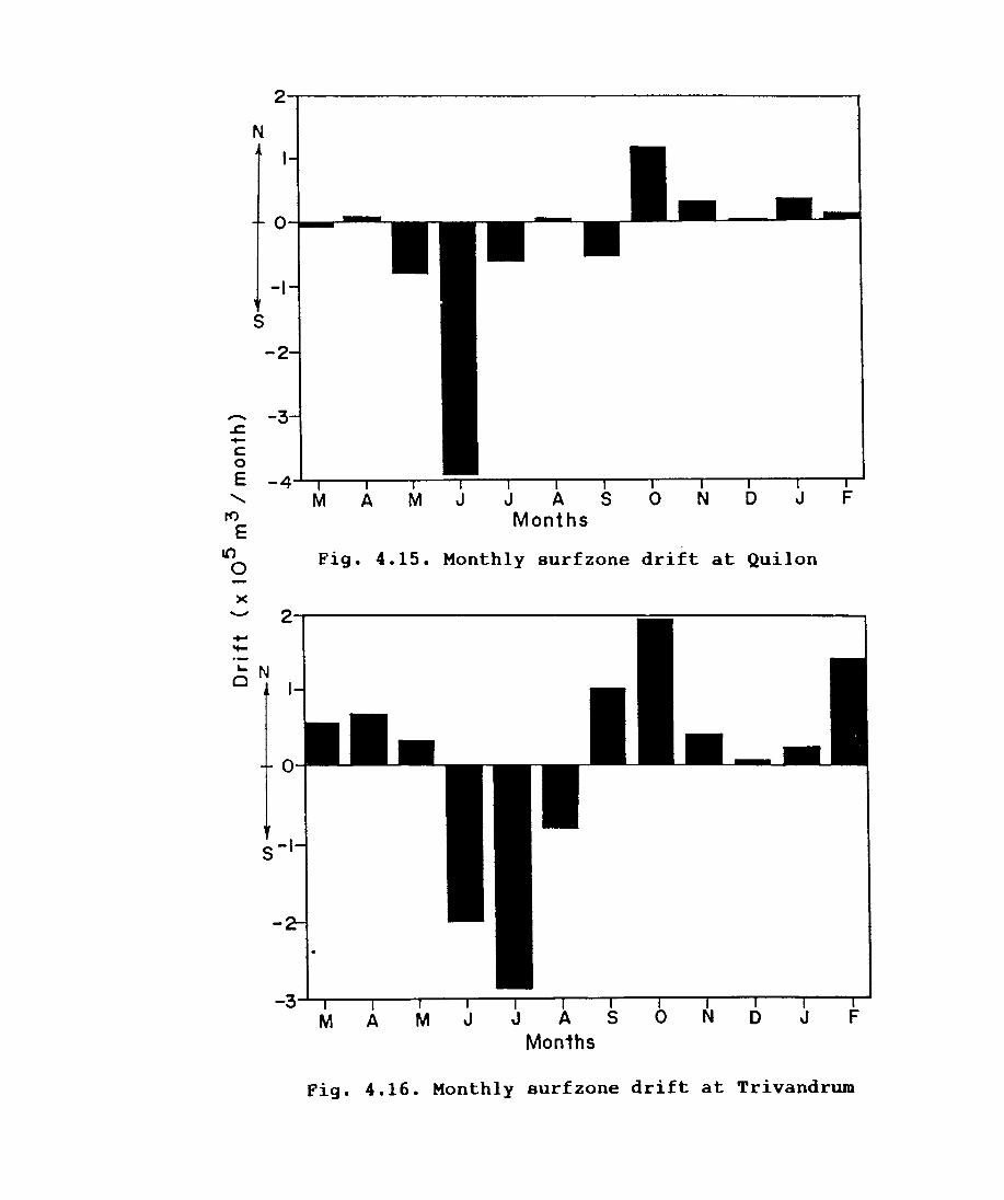
2.-------------------------------------------~

N

0-'------

-I

S

- -.s:: -£:: o E -d~_r--~--~~~~,_--~--~--~--~--~--~--~

" rt)

E 10 o )( -'- N

Cl

Fig. 4.15. Monthly Burfzone drift at Quilon

Fig. 4.16. Monthly Burfzone drift at Trivandrum

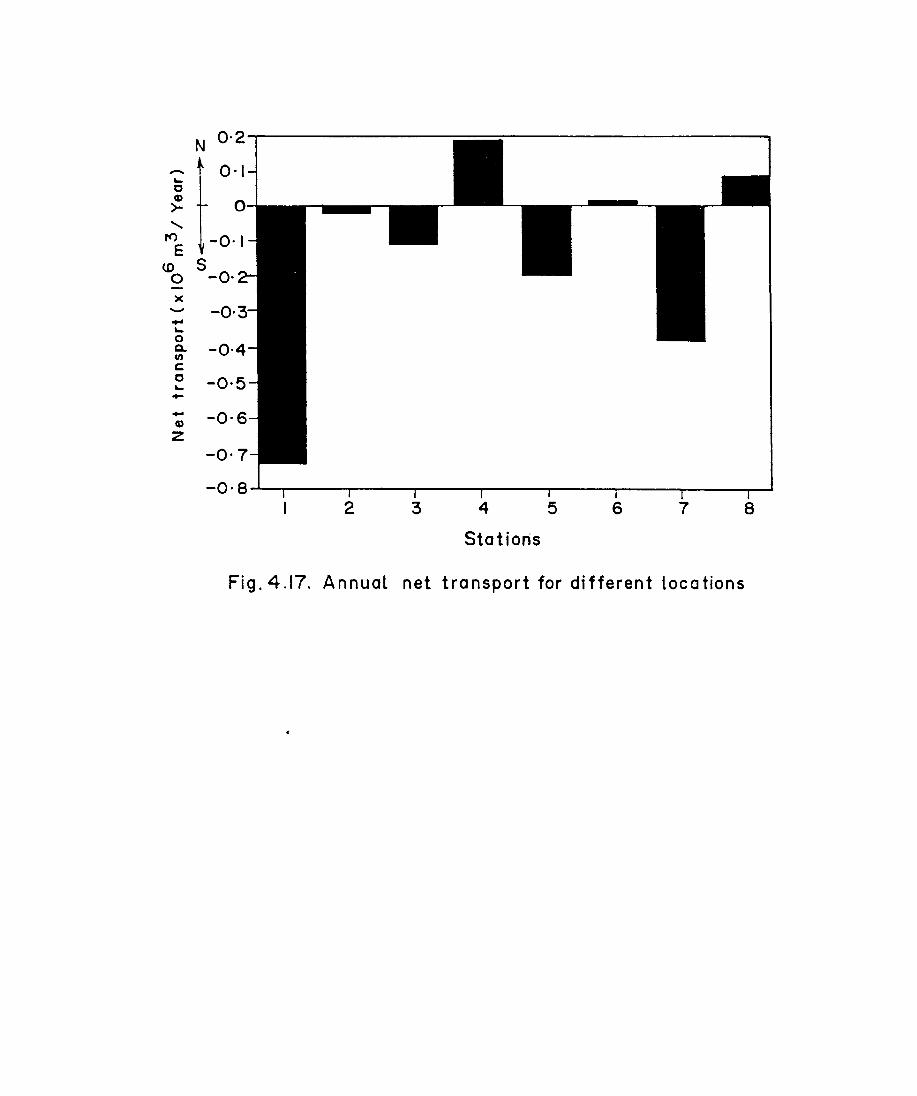
N 0·2

- 0·1 ~

0 Q)

>-.......

tt)

E to

0 x --~ 0 Q. Cl)

C 0 ~ -- -0· Q)

z

2 3 4 5 6 7 8

Stations

Fig.4.17. Annual net transport for different locations

. I f 3 91 X 10 5 3. J maX1mum va ue o. m 1n une. The magnitude of

drift values shows a decreasing trend towards September

followed by a shift in direction. The lowest northerly drift

value of 0.023 X 10 5 m3 is observed during December. The

annual net transport 1S towards south with a magnitude of

0.38 X 106 m3 .

The estimated value of the monthly drift for the

Trivandrum beach (Fig. 4.16), shows higher magnitude than at

Quilon beach. The drift is southerly only during the south-

west monsoon period (May-September) and northerly in other

months. The higher magnitude of the drift values along this

beach is due to the high energy conditions prevailing along

this beach. From the monthly and daily wave breaker height

analysis (Chapter 4, Section 4.1.2), it is evident that this

beach has all typical characteristics of a high energy beach.

with the onset of monsoon, an increase in southerly drift

value is observed and shows a maximum value in July (2.87 X

10 5 3 m ). As reported from earlier studies, during the onset

of south-west monsoon season, breaker directions mostly vary

between 230 0 - 240 0 causing a southerly longshore current and

a southerly drift. During post-monsoon months an increase in

drift value is observed with a maximum of 1.93 X 10 5 3 m in

October and is northerly. The reversal in drift direction is

very conspicuous in this beach. Annual net drift along this

6 3 beach is towards north with a low value of 0.09 X 10 m.

90

CHAPTER 5

5. SUMMARY AND CONCLUSIONS

A coastline represents a dynamic, fragile physical and

biological environment that is constantly changing in

response to natural processes as well as human activities. It

holds great attraction for man as it provides him with a

variety of resources for food, construction, recreation,

transportation and aesthetics. It also provides a natural

protective barrier for inland areas against violent storms as

well as daily or seasonal attacks by wind and waves. For many

years, studies of coastal processes and landforms were

attempted to gain a better understanding of the complex

interaction between land, air and water.

The nature and behavior of a coastal system depend on

the character, frequency and intensity of the input energy

and on the configuration and composition of the subaquous and

subaerial boundaries. Regional and local scale variations in

~oastal dynamic regimes and resultant morphologies reflect

the complex mutual interactions between these energy inputs

and boundary configurations.

Beach dynamics of the Kerala coast has been studied to

delineate the physical processes along the different types of

beaches representing the open coast beaches, beaches with

headlands, barrier types, beaches exposed to high and low

energy environments and beaches protected by the occurrence

of mudbanks. Each type has been viewed as a representative

entity for estimating different coastal processes.

91

The high energy beach at Kasargod, shows maximum

variability in the foreshore region. The E.O.F analysis as

well as the beach volume changes show that the beach exhibits

cyclic episodes of erosion and accretion in response to the

monsoon and fair w~~Lher seasons. The storage volume of the

beach is maximum (765 m3 /m) at the beginning of the study,

during March 1990 and shows the least storage volume (704

m3 /m) in September 1990 when it is subjected to maximum

erosion. However the erosion to which the beach is subjected

to, occurs in three phases. After the cessation of south-west

monsoon, the beach builds up gradually. By the end of the

study period (February 1991), the beach regains to only 738

3 m Im in storage volume. The mean grain size of the sediment

sample, collected from the low water line sample of Kasargod

beach, shows that it belongs to coarser grade sand size

class, moderately sorted and negatively skewed. Coarsest

material occurs during August, coinciding with the erosion

·during the south-west monsoon period. The skewness is

directly related to the erosional/accretional pattern of the

beach (King, 1972). The negative skewness values observed

most of the time, indicates the erosional phase of the beach.

The symmetrical skewness seen during September to November

indicates the accretional phase of the beach. Monthly

littoral drift values show that the drift values are maximum

compared to the other locations and are oscillatory in

nature. The maximum southerly drift is about 2.95 X 3 m

during June. Incidentally, this is the time when the beach

92

starts eroding considerably. This maximum drift is brought

about by the prevailing high wave energy at this location

associated with the south-west monsoon which is aJso evident

from the LEO data discussed in (Section 4.1.2). The magnitude

of the annual net drift is 0.73 X 106 m3 and is towards

north.

The Payyambalam beach at Cannanore in the vicinity of

Ezhimala promontory is a straight long beach with seawall at

the backshore. The beach exhibits typical monsoon response by

way of erosion during both south-west (June-July) and north-

east (October) monsoons. Maximum erosion occurs during July

when the storage volume is least (412.5 3 m Im). Over the

period of one year the beach almost regained its initial 3 .

storage volume of 442 m Im by March 1990. In general, though

the beach has undergone seasonal erosion during monsoon, it

receives its lost material thereby maintaining an equilibrium

state. For most of the time, the beach sediment is 1n the

medium sand class. The moderately well sorted sediments with

negatively skewed occurring during the south-west monsoon

indicates the erosion and the symmetrical skewness with poor

sorting during the fair weather season indicates bui.lding up.

The monthly littoral drift values show a maximum southerly

direction during August (1.38 X 10 5 m3 ) when it is southerly.

Annual net littoral drift is towards south with a magnitude

of 0.019 X 106 m3 •

Konad beach at Calicut, sheltered by the mud bank is

wide and sandy with least variability compared to the rest of

93

the beaches. This beach also responds, though to a lesser

degree, to the south-west and north-east monsoons undergoing

erosion both during July and October. Accordingly the changes

in storage volume also are minimal to the tune of 10 m3 /m

during the south-west monsoon and 5 m3 /m during the north-

east monsoon. The beach regains it's initial storage volume

of 1302 m3 /m (April 1990) by the end of January 1991. The

stable nalure of the beach is very clearly depicted in the

E.O.F analysis also. The mean size of the beach sediment

belongs to medium sand class without much variations over

this period showing the low energy environment. Coarser

grain size class, which is highly sorted and negatively

skewed shows the erosional behavior of the beach during the

north-east monsoon. The low value~ of the medium grain size

during south-west monsoon along with small volume changes are

caused by the calm conditions provided by the dampening of

waves under the influence of the Calicut mud bank. The

breaker height distribution also confirms the results. The

monthly drift at this location shows that the magnitude of

the littoral drift is low compared to the other northern

locations. The maximum drift occurs during March (0.76 X 10 5

m3 ) and is southerly. The low values observed during the

south west monsoon is due to the occurrence of mud bank. The

minimum monthly drift value of 0.11 X 10 5 3 m is observed

during the north-east monsoon season (November). The annual

net drift is southerly with a magnitude of 0.Oi1 X 6 3 10 m

indicating the stable nature of the beach. The supply of

94

sediments from the rivers on either side of the beach also

provides stability to the beach.

. The Nattika beach is an open straight beach backed by

seawall well inside the backshore. The storage volume shows

that the beach has maximum material in the beginning of March

1990 (548 m3/m) with a rapid erosion during the onset of the

south-west monsoon. The beach loses about 34 m3 /m of the

material within two months of south-west monsoon (,June and

July). It takes about six months for the beach to recover its

lost material reaching 544.7 m3 /m by January 1991. Then

onwards the beach continues to accrede to a storage volume of

557.0 3/ m m in February 1991. In contrast to the other

beaches, this beach does not show any erosion during north-

east monsoon. Thus, in general, the beach shows an

accretional trend over the period of study. The existence of

an old seawall well behind the backshore is a good indication

of the building up nature of the beach during the past years.

The mean grain size shows that the beach material belongs to

fine sand class during most part of the year with some

exceptions during September-October when it shows medium

sand. The sediment shows well sorted to moderately sorted

nature with symmetrical skewness indicating the accretional

trend of the beach. The monthly drift at this beach shows a

southerly direction during the monsoon months with the

maximum drift occurring during September (0.78 X

3 m /month). This beach depicts the typical monsoon sediment

drift pattern. However, during November to February, the

95

drift is towards north. In general, the monthly drift values

at this beach are higher than at the Calicut beach. This may

be due to the wide surf zone which causes to set more sand in

motion. Annual net drift shows a northerly drift with values

of 0.19 X 106 m3 •

Andhakaranazhi beach is a barrier type short beach.

The storage volume shows that before the onset of south-west

monsoon, the beach has a storage volume of 587 m3 /m (April)

which rapidly 3 decreases to 35 m Im during June under the

action of high monsoonal waves. The accretion is also rapid

and the beach regains its material by the end of October 1991

(582 m3 /m). The influence of the north-east monsoon also is

seen in the beach volume during November-December which shows

3 a loss of material to the tune of 7 m Im. However, the beach

regains this material by the end of February. Thus the

storage volume as well as the results of the E.O.F analysis

shows the near-stable nature of the beach during this period.

The average grain size shows the presence of medium grade

sand. Beach shows fine sand class till the end of July. The

presence of medium sand during north-e~st monsoon indicates

the eroding phase of the beach. The sediments show a well

sorted nature during the south-west monsoon period and poorly

sorted nature during north-east monsoon. The symmetrically

skewed nature of the sediment during most of the time shows

almost stable nature of the beach. The monthly littoral drift

values along this beach also shows a monsoon trend of

southerly drift with a maximum value of 1.11 X 10 5 3 in m

96

June. In all the other months, except during March and

January and monsoon months, the drift is towards north.

Annual net drift shows a southerly drift with ? magnitude

6 3 0.2 X 10 m.

The Alleppey beach is a wide and long beach with the

sheltering provided by the mud bank during the south-west

monsoon period. During the period of survey Alleppey mud bank

was active with calm waters and heavy load of mud in

suspension. (Joseph, 1992). The storage volume shows that the

beach continuously builds from it's March level of 895 3 m Im

to 942 m3 /m during August. Thus 3 material about 47 m Im of 1S

accreded during these six months. The north-east monsoon

effe~t is seen during October when the beach volume reduces

by about 15 m3 /m. The occurrence of mud bank in this region

during the south-west monsoon dampens the high monsoonal

waves and makes this nearshore very calm. The southerly drift

from the beaches north of Alleppey gets trapped by the mud

bank leading to the observed accretion. The E.O.F analysis

and grain size composition also show the accretional nature

of the beach. The poorly sorted distribution along with

negative skewness during the north-east monsoon indicates an

erosional trend. However the symmetrical skewness during the

rest of the period indicates accretional nature of the beach.

The monthly littoral drift shows lesser values even during

the peak monsoon months sUbstanciating the results obtained

from beach volume and grain size studies. It shows the low

energy environment prevailing over this location brought in

97

by the mud bank. The maximum northerly drift of 0.13 X 10 5 3 m

is observed during April. Subsequently the drift shows

southerly direction during the south-west monsoon season.

During the north-east monsoon season the drift becomes

negligible with a value of 0.0011 X 10 5 m3/month during

November. The annual net littoral drift (0.016 X 106 m3 /year)

is the least and is directed northerly.

The Quilon beach, south of Thankasseri headland, is a

narrow beach. During the south-west monsoon, the beach erodes

rapidly loosing about 54 m3 /m of the beach material from it's

initial storage volume of 425 m3 /m in April 1990. By the end

3 of the survey the beach has only 404 m Im of storage volume,

indicating a net deficiency of about 21 m3 /m of the material.

Thus the beach at Quilon undergoes erosion as also evident

from the E.O.F analysis. The mean grain size shows the

presence of coarser sand most of the time. It shows coarsest

sediment during the south west and north-east monsoon seasons

with poor sorting. The intensive sand mining activity, for

black sand, along this stretch of the beach could be a factor

affecting the long-term equilibrium of this beach. The

littoral drift shows higher values compared to Alleppey beach

with a maximum drift of 3.91 X 105 m3 towards south in June.

It shows a typical monsoonal character ~ith southerly drift

during south-west monsoon period and northerly drift during

rest of the year. The annual net drift is southerly with a

magnitude of 0.38 X 106 m3 •

98

_G'7300 -

Shankhumukham beach at Trivandrum is an open beach

exposed to high wave energy. This beach shows typical monsoon

response by way of erosion during June-July. From the storage

volume, it is seen that the beach loses 67 m3 /m of the

material during monsoon period when the beach is subjected to

very high wave energy environment. The erosion is rapid while

the accretion is gradual and steady taking about 4 to 5

months to recover the material lost during the south-west

monsoon. By

considerable

the end of the survey the beach

building up (478 m3/m) compared to its

shows

initial

volume of 466 m3 /m before the onset of monsoon. The average

grain size shows the presence of medium grade sand during the

entire study period. Sorting value shows moderately well

sorted material to moderately sorted during south-west

monsoon. The sediment is symmetrically skewed throughout the

entire period which shows that the beach accretes during the

survey period. The monthly littoral drift values show

comparatively higher magnitudes compared to the beaches at

central part, which is due to the prevailing high energy

environment at this location. The beach show monsoonal

behaviour of southerly drift with a maximum value of 2.87 X

3 m

northerly

in July. Annual net drift along this beach was

with a magnitude of 0.09 X 106 m3 . The the volume

changes as obtained from the storage volume studies also

indicate this.

It is observed that the wave heights are high at some

locations and lower at other locations along the coastline of

99

Kerala. This kind of wave height distribution is associated

with the formation of zones of convergence of wave energy at

locations with higher waves and zones of diverg~nce of wave

energy at locations with lower wave heights.

It is interesting to note that the wave convergence

at Vypin is a permanent feature which occurs for waves from

all directions.

The divergence of wave energy seen south of Ezhimala

promontory for o 270 and 8 S. The divergence at Cannanore,

Badagara and Mahe is caused by the presence of Ezhimala

promontory The divergence at Quilon and Varkallai for wave

direction 290 0 and period 8 S is due to the presence of

headland at Thankasseri •

The presentation of refraction coefficient and net

wave height graphs can be used as monograms for evaluating

the wave height for different deep water wave heights along

the Kerala coast.

The Kasargod beach, shows an eroding nature over the

period of study and indicates the monsoon response of erosion

during both the monsoons. The Payyambalam beach at

Cannanore, in the vicinity of the Ezhimala promontory shows

an overall stable nature. The presence of promontory seems to

modify any waves approaching the coast from north and protect

the oeach. This beach responds to both' the monsoons with

erosion and with accretion during the other months. The

erosion seen at Kasargod may be in part due to the effect of

100

promontory

beach at

promontory.

which prevents the northerly drift.

Kasargod gets only sediments which

The high littoral drift value at

Hence

bypass

Kasargod

the

the

is

indicative of larger sediment supply brought in by the high

wave energy and the influx of sediments owing to the

existence of rivers draining along this coast. The Konad

beach at calicut shows the least variability during the

period of study. The drift values are also very low here,

showing minimum variability. This beach shows monsoonal

responses to a very lesser degree. Nattika beach shows

monsoonal erosion during south-west monsoon and accretion

during north-east monsoon. Andhakaranazhi beach shows stable

nature and it shows erosion only during south-west monsoon

and an accretional trend during the north-east monsoon.

Alleppey beach shows accreding trend even during the south

west monsoon with slight erosion during north-east monsoon

season. This beach shows a typical mud bank response with

accretion during the south-west monsoon season and a slight

erosion during the north-east monsoon. Quilon beach shows

typical monsoonal erosion during both the monsoons.

Trivandrum beach, exposed to high energy environment shows

high variability of beach volume. The beach responds well

with erosion during south-west monsoon and during the north­

east monsoon it shows a strong accretional trend.

The beach variability of the northern and southern

beaches are maximum as compared to the central beaches

because the former are exposed to high wave energy and the

101

latter are either protected by mud banks or are low energy

beaches. The northern beaches show northerly net drift while

the central beaches show southerly drift. The southerly

beaches show an oscillatory type drift characteristics.

The temporal distribution of the third eigen function

depicts the temporal fluctuations of the positions of the low

water mark. The lowest positive peak of the V3 curve

coincides with the minimum proximity of the position of the

low water line from the bench mark and the lowest negative

value coincided with the maximum distance of the low water

line from bench mark, which reflects the erosional and

depositional phases respectively. This temporal variability

may be attributed to the spatial variability of the interplay

between locally generated winds, waves, tides, currents and

the bottom topography.

Four different types of relations were tested for the

monthly data sets of storage volume against the corresponding

drift values.

1 • y = -126.459075 X + 736.228955 (r=0.29,Variability=0.08)

2. y = -71.30008 LOG(X) + 550.64295 (r=0.45,Variability=0.20)

3. y 676.65959 -0.175061 X (r=0.30,Variability=0.09) = e

4 . Y = 525.140731 X-·096641 (r=0.46,Variability=0.21)

Of these, Y = 525.140731 x-·096641 (Fig. 5.1),

explains comparatively a better amount of variability. A

major part of the variability rema1ns unexplained which

requires detailed investigations as suggested below.

102

103 :" 1300.00 It <I... .

Fig. 5.1. Relation between monthly drift and storage volume

5.1. Scope for future study

Though the studies on the beach changes along this

coast have been conducted, it is still necessary to monitor

the beaches in this region continuously over an extended

period of time with an increased number of close study

locations, in order to establish a more reliable quantitative

predictive model for the Kerala coast. The environmental and

economical significance of an improved quantitative

predictive model justifies the improvement of substantial

future field programs. Further studies are needed to

establish the estimation of effective nearshore transport of

sediments using Littoral Environmental Observation (L.E.O),

under varying environmental conditions.

REFERENCES

REFERENCES

Achuthapanickar, G., 1971. Coastal protection works at Chellanam and Vypeen, Proc. of the ~. on coastal 'erosion and protection. KERI, Peechi: 10.1-10.11.

Ahmad, E., 1972. Coastal Geomorphology of India: 222 p.

Airy, G.B.,1845. On tides and waves, Encyclopedia Metropolitana.

Ananthakrishnan, R., Parthasarathy, B. and Pathan, J.M., 1979. Meteorology of Kerala. In:G.S. Sharma, A. Mohan Das and A. Antony. (Ed). Contribution to Marine Sciences, (Dedicated to C.V. Kurian): 60-125.

Andhra University, 1954, Memoirs in oceanography, V.1, Waltair, Andhra University.

Andhra University, 1958, Memoirs in oceanography, V. 2, Waltair, Andhra University.

Anonymous" 1975. Shore Protection Manual, Vol.1, Coast. Engg. Res. Centre, U.S. Army Corps. of Engg.: 514.

Anonymous., 1974. Public works department (Kerala), Water Resources of Kerala, Govt. of Kerala Publication, Tvm.

Antony, M.K., 1976. Wave refraction off Calangute Beach, Goa, with special reference to sediment transport and rip currents. Indian Journal of Marine Sciences, 5(2):1-8.

Aranuvachapun, S. and Johnson, J.A., 1979. Beach profiles at Gorleston and Great Yarmouth. Coastal Engineering, 2: 201-213.

Arthur, R.S., Munk, W.H. and Issacs, J.D., construction of wave rays. Trans. Amer. 33: 855-865.

1952. The Geophys.

direct Union,

Aswathanarayana, U., 1964. Origin of the heavy mineral beach sand deposits of the south-west coast of India. Advanced frontiers in geology and geophysics: 481-489.

Aubrey, D.G., 1978. Statistical and dynamical prediction of changes in natural sand beaches. Ph.D. dissertation, Scrips Institute of Oceanography, California: 194 pp.

Aubrey, D.G., Inman, D.L. and Nordstrom, C.E., 1976. profiles at Torrey Pines, California. Proc. 15th Conf. Coastal ~, Honolulu, Hawaii: 1277-1296.

Beach Int.

1979. Seasonal patterns of onshore / offshore movement. Journal of Geophysical Research, 84:

Aubrey, D.G., sediment 6347-6354.

104

Baba,

Baba,

M., 1979b. Coastal erosion in Kerala - Some problems solutions. Professional Paper. No.6, CESS, Trivandrum.

M., 1981a. Impact of coastal and harbor structures on coastal environment of Kerala, Proc. Seminar 2Q status environmental studies in India, Trivandrum: 65-72.

and

the of

Baba, M., 1985. Long-term wave monitoring along the Kerala coast­some results. Proc. Nat. Conf. on Dock and Harbour ~., lIT, Bombay: E 49-67.

Baba, M., 1986. Kerala's coastal zone - a management proposal, Technical Report, C.E.S.S, 47: 27.

Baba, M., 1987. Wave power potential off the southwest Indian coast, Energy, 12(6): 501-507.

Baba, M., 1988. Wave characteristics and beach processes of the south west coast of India - a summary. In: Ocean waves and beach processes. M.Baba and N.P.Kurian (Eds.), CESS, Trivandrum: 225-239.

Baba, M., 1988a. Ocean wave research in India.ln: Ocean waves and beach processes. M. Baba and N.P. Kurian (Eds.), CESS, Trivandrum: 1-14.

Baba, M. and Harish, C.M., 1986. Wave energy spectra for the southwest coast of India, Indian Journal of Marine Sciences, 15: 144-152.

Baba, M., Shahul Hameed, T.S., Kurian, N.P., Thomas, K.V., Harish, C.M., Joseph, P.S., Prasannakumar, M. and Varghese, K.K., 1985. Wave climatology for the south-west coast of India. Paper presented at the Symposium on Concepts and Techniques in Applied Climatology, Waltair.

Baba, M., Shahul Hameed, T.S., Kurian, N.P., Thomas, K.V., Harish, C.M., Rameshkumar, M and Mohan, S., 1991. Long­term wave and beach data of Kerala coast - Part I :1980 '84, Technical Report No. 57, C.E.S.S, Tvm.

Baba, M., Thomas, K.V., Hameed, T.S.S., Kurian, N.P., C.E., Abraham, S. and Rameshkumar, M., 1987. Wave and power off Trivandrum. In:Report for ~ trial Kw wave energy device, 0.0.0, Govt. of India.

Bagnold, R.A., 1963. Beach and nearshore processes Mechanics of marine sedimentation. The Sea, Ill, Wiley: 507-528.

Rachel, climate

of a 150 -- - ---

Part I, Newyork,

Bascom, W.N., 1954. Characteristics of natural beaches. Proc. 4th Int. Conf. Coastal Engineering: 163-180.

Bascom, W.N., 1980. Waves and Beaches, Ancher Books, Newyork:267p.

105

Boussinesq, J., 1872. Theory of waves and swells propagated in a long horizontal rectangular canal and imparting to the liquid contained in this canal approximately equal velocities from the surface to the bottom, Journal de Mathematiques Pures et Appliquees, Vol. 17, Series 2.

Bowen, A.J., 1969. The generation of longshore currents on a plane beach. Journal of Marine Research: 206-215.

Brunn, P., 1954. Coast erosion and the development of beach profiles. B.E.B. Tech. Memo.

Caldwell, M.J., 1956. Wave action and sand movement near Anaheim Bay, California, U.S. Army Beach Erosion Board, Tech. Memo. No.68 : 21p.

Chandramohan, P., 1988. Longshore sediment transport model with particular reference to Indian coast, Ph.D. Thesis, I.I.T, Madras.

Chandramohan, P. and transport along Marine Sciences,

Nayak, B.U., 1991. the Indian coasts.

20(2): 110-114.

Longshore sediment Indian Journal of

Chandramohan, P., Nayak, B.U. and Pathak, transport along the Indian coast. 6/89.

R.C., 1989. NIO-Technical

Sediment Report-

Chandramohan, P. and Narasimha Rao, T.V., 1984. study of longshore current equation for currents in Visakhapatanam Beach. Indian Journal of Marine Sciences, 13: 24-27.

Chandramohan, P., Narasimha Rao, T.V. and Panakala Rao, D., 1981. Studies on the beach changes. at Visakhapatnam, Mahasagar - Bulletin of Nat. Inst. Oceanography, 14(2) 105-115.

Chandramohan, P. and Rao, R.P.R., 1985. Mathematical prediction of long term shoreline changes at Vishakhapatnam. J. Inst. Engrs. (India), 66(CI 3&4): 121-128.

Chandramohan, P., Sanil Rumar,V., Nayak, B.U. and Anand, 1990. Wave Atlas for the Indian Coast (Based on --- ---observations, 1968 - 1986).

N.M., ship

Chandramohan, P., Sanilkumar, V. and Nayak, B.U., 1991. Wave statistics around the Indian coast based on ship observed data, Indian Journal of Marine Sciences, V. 20: 87-92.

Chandramohan, P., Sanilkumar, V. and Nayak, B.U. and Pathak, R.C., 1993. Variation of longshore current and sediment transport along the Maharashtra coast, West coast of India. Indian Journal of Marine Sciences, 22: 115-118.

106

Chappell, J. and Elliot, I.G., 1979. Surf-beach dynamics in time and space - an Australian case study, and elements of a predictive model. Mar. Geol., 32: 231-250.

Chaudhri, R.S., Khan, H.M.M. and Kaur, S., 1981. Sedimentology of beach sediments of the west coast of India.' Sediment. Geol., 30: 79-94.

Chavadi, V.C. and Bannur, C.R., 1992. Beach profile study along Ramangudi beach of north Karnataka coast. (West coast of India). Indian Journal of Marine Sciences, V. 21:107-110.

Clarke, D.J., subareal over a

Eliot, I.G. and Frew, J.R., 1984. beach sediment volume on a small

monthly lunar tidal cycle. Marine

Variation in sandy beach

Geology, 58: 319-349.

Curt.D. Peterson., Phillip.L. Jackson., Douglas.J. 0' Nest., Charles.L. Rosenfeld. and A. Jon Kimerling., 1990. Littor­al cell response to interannual forcing 1983 -1987 on the central Oregon coast, USA, Journal of Coastal Res., 6(1): 87-110.

Das, P.K., Hariharan, V. and Varadachari, V.V.R., 1966. Some studies on wave refraction in relation to beach erosion along the Kerala coast. Proceedings of Indian Academy of Sciences, LXIV: 192-202.

Dattatri, J., 1973. Waves of Mangalore harbor-west India. Journal of Water ways, Harbor and Engineering division, ASCE 99(WWI): 39-58.

coast of Coastal

Dattatri, J. and Ramesh, C.R., 1972. Study of equilibrium profiles, J. Inst. Engrs. India, 52 (Cl 5): 140-145.

Dattatri, J. and Renukaradhya, P.S., 1971. Wave forecasting west coast of India, Journal of Waterways, Harbors Coastal Engineering, ASCE, 97: 505-515.

beach

for and

DingIer, J.R., 1981. Stability of a very coarse grained beach at Carmel, California. Marine Geol., V. 44: 241-252.

Dhanalakshmi, S., 1982. Wave refraction and nearshore circulation at Visakhapatnam, Indian Journal of Marine Sciences, 11:153-158.

Dobson, R.S., 1967. Some applications of digital computer to hydraulic engineering problems, Dept. of civil engineer­ing, Stanford University, Technical report. No.80: 115 p.

Dolan, R., 1965. Seasonal variations in beach profiles along the outer banks of North Carolina beach, Oct.

Dora, Y.L., Damodaran, R. and Jos Anto, V., 1968. Grain Slze of

107

the Njarackal mud bank sediments. Symp. Coastal erosion and protection, Ker. Eng. Res. Inst •. 23: 5p

Eliot, I.G., 1974. Relationship between nearshore water circulat­ion and sandy beach morphology at Durras, New South Wales, Ph. ~ Thesis, Geogr. Dept, S.G.S, Canberra.

Folk, R.L. and Ward, W.C., 1957. Brazos river bar, A study in the significance of grain size parameters, ~ Sed. Petrol, 27: 3-27.

Frew, J.R., Elliot, I.J. and Clarke, D.J., 1983. Day to day variation in nearshore bar patterns through a lunar tidal cycle on a small sandy beach. Aust. Geogr. Studies.

Friedman, G.M., 1967. Dynamic processes and statistical parameters compared to size frequency distribution of beach and river sands. ~ Sed. Petrol, 37: 327-354.

Galvin, C.J., 1972. A gross longshore transport rate formula, Proc. 13th Coast. Engg. Conf., 2: 953-969.

Giles, R.T. and Pilkey, O.H., 1965. Atlantic beach sediments of the southern united states. J. Sed.

and dune Petrol. , ---

V. 35: 900-910.

Goldsmith, V., Sturm, S.C. and Thomas, G.R., 1977. Beach erosion and accretion at Virginia beach and vicinity, U.S Army Crops of Engineers, CERC Miscellaneous Report, MR 77-12: 185p

Gopinathan, C.K. and Qasim, S.Z., 1974. Mud banks of Kerala Their formation and characteristics, Indian Journal Marine Sciences. 3(4): 105-114.

of

Gopinathan, C.K., Sathe, P.V. and Ramaraju, power around southern coast of India October, 1977, Mahasagar, 12: 135-140.

D. V. , during

1979. Wave September-

Gouveia, A.P., Joseph, P.S. and Kurup, P.G., 1976. refraction in relation to beach stability along coast from Cape Ramas to Karwar. Mahasagar - Bulletin Na~i. Inst. Oceanography., 9(1): 11-18.

Wave the of

Graff., V.D. and Overeem, V.J.,1979. transport formulae in coastal Coastal Engineering, V.3: 1-32.

Evaluation of sediment engineering practice,

Griswold, G.M., 1963. Numerical calculation of wave refraction, Journal of Geophysical Research., 68(6): 171~-1723.

Hanamgond, P.T. and Chavadi, V.C., 1993. Sediment movement on Aligadde beach, uttara Kannada district, West coast of India, Journal of Coastal Research, 9(3): 847-861.

108

Harish, C.M., 1988. Waves and related nearshore processes complex Bay beach at Tellichery, Ocean Waves and processes, C.E.S.S, Trivandrum: 111-127.

in a Beach

Harish, C.M. and Baba, M., 1986. Spectral ang statistical properties of shallow water waves, Ocean Eng., 13(3): 239-248.

Hameed, T.S.S., 1988. Wave climatology and littoral processes at Alleppey. In: Ocean waves and beach processes, C.E.S.S: 67-90.

Hameed, T.S.S., Baba, M. and Thomas, K.V., 1986. Computation of longshore current. Indian Journal of Marine Sciences,15: 92-95.

Harrison, W. and Wilson, W.S., 1964. Development of a method for numerical calculation of water refraction. U.S Army Crops of Engineers, CERC, TEchnical Memo No. 6.

Hastenrath, S. and Lamb, P.J., 1979. Climatic atlas of Indian Ocean-Part I Surface climatic and atmospheric calculation, The university of Wiscon press.

Horikawa, K., 1978. Coastal Engineering, An introduction to ocean engineering, (University of Tokyo Press, Tokyo): 273.

Ingle, J.C., 1966. The movements of beach sand. Developments in sedimentology, V. 5: 221p.

Inman, D.L. and Bagnold, R.A., 1963. Littoral processes. In The Sea, Vol. 3, M.N. Hill, (Ed.), Interscience, Newyork: 529-553.

Inman, D.L. and Fratuschy, J.D., 1966. Littoral processes and the development of shorelines. Coastal Engineering., Santa Barabara Speciality Conf. : 511-536.

Ippen, A.T., 1966. Estuary and Coastline Hydrodynamics, Engineer­ing Societies Monograph, Mc Graw - Hill, Newyork:744p.

Isobe, M., 1985. Calculation and application of first order cnoidal wave theory, Coastal Engineering, Vol. 9: 309-325.

Iwasa, Y., 1955. Analytical consideration on solitary waves, Memoirs of the Faculty of University, Japan.

cnoidal and Engg., Kyoto

Jacob, V.C., 1976. Geology of Quilon district. Geol. and Geomorph. Kerala, Geol. Surv. India.

Jen, Y., 1969. Wave refraction near San Pedro Bay, California. J. of Waterways and Harbor division., ASCE, WW3: 379-393.

109

John, J.E. and Padmanabhan, H., 1971. History of Kerala shore, J. Inst. Engrs. India, 51.

John, J.E. and Verghese, G., 1976. Shoreline changes on Kerala coast. Proc. of Seminar on Geology. and Geomor­phology of Kerala. Trivandrum.

John, J.E. and George, V., 1980. Shoreline changes on the Kerala coast. In: Geology and geomorphology of Kerala, G.S.I, Special publication, 5: 83-85.

Johnson, J.W., 1947. The refraction of surface waves by currents. Trans. American Geophys. Union, 28(6): 867-874.

Johnson, J.W., 1956. Dynamics of nearshore sediment movement Bull. Amer. Assoc. Petrol. Geol. 40: 2211-2232.

Joseph, P.S., 1984. Prediction of cyclone generated waves along Indian coasts. Vayumandal, 14(3&4): 40-46~

Joseph, P.S., Mohanan, S. and Varghese, K.K., 1984. Pre-monsoon wave conditions off Vizhinjam harbor in 1984. Bull. Pure Appl. Sci., 3C(2): 53-58.

Joseph, M., 1992. Wave-mud interaction in mudbanks. Ph.D. Thesis, Submitted to the Cochin University of Science and Technology.

Kanth, T.A., 1984. The longshore transport of sand on Puri and Madras beaches, Ph. ~ Thesis.

KERI., lQ71. Coastal erosion in Kerala state problems and remedy, Official paper, Irrigation, Kerala st.

Brochure on Chief Eng.

Keulegan, G.H. and Patterson, G.W., 1940. Mathematical theory of irrotational translation waves, Report No. 1272, National Bureau of Standards, Washington, D.C: 47-101.

Keulegan, G.H., 1948. Gradual damping of solitary waves, Journal of Research, National Bureau of ·standards, Vol. 40 480-498.

King, C.A.M., 1972. Beaches and Coasts, Arnold Ltd., London: 569p-.--

( 2nd ed.), Edward

Komar, P.D., 1976. Beach Processes and Sedimentation, Prentice­Hall, Inc., Englewood Cliffs~ew Jersey:429 pp.

Komar, P.D. and beaches.

Inman, D.L., 1970. Longshore sand transport J. Geophys. Res., 75: 5914-5926.

on

Korteweg, D.J. and deVris, G., 1895. On the range of form of long waves advancing in a rectangular canal and a new type of

110

long solitary waves, Philosophical Magazine, 5th series: 422-443.

Krishnan, M.S., 1968. Geology of India and Burma, 6th Ed., Higginbothams, Ltd., Madras: 64p.

Krishnakumar, V., Murty, C.S., Shenoi, S.S.C. and Heblekar., 1989. Wave refraction and longshore current patterns along Calangute beach (Goa), West coast of India. Indian Journal of Marine Sciences. 18: 184-188.

Krumbein, W.C., 1944. Shore processes and beach characteristics, Beach erosion board, Tech. Memo. 5(3).

Kurian, N.P., 1987. Wave height and spectral transformation in the shallow waters of Kerala coast and their prediction, Ph.D. Thesis, Cochin University of Science & Technology.

Kurian, N.P., 1988. Waves and littoral processes at Calicut, In: Ocean waves and beach processes, CESS, Trivandrum: 91-110.

Kurian, N.P., Baba, M. and Hameed, T.S.S., 1985a. Prediction of nearshore wave heights using refraction programme, Coastal ~, 9: 347-356.

Kurian, N.P., Hameed, T.S.S. and Baba, M., 1984. Beach in relation to wave climate at Alleppey, CESS Report No. 38.

dynamics Technical

Kurian, N.P., Hameed, T.S.S. and Baba, M., 1985. A study monsoonal beach processes around Alleppey. Proc. Acad. Sci. (Earth Science), 94: 323-332.

of Ind.

Kurup, P.G., 1974. Coastal zone management Problems and prospects for Kerala. Sea food export Journal, 6(12):45-48.

Kurup, P.G., 1977. Studies on the physical aspects of the mud banks along the Kerala coast with special reference to Purakad mud bank, Bull. Dept. Mar. Sc. Univ., Cochin, 8: 1-72.

La Fond, E.L. and Prasad Rao, R., 1956. On the erosion of the beach at Uppada. The port ~., V. 5: 4-9.

Lalithananda Prasad, Lakshmana Rao, Sciences, 10.

A. Hanumantha Rao, K., Veenadevi, Y. and G.R., 1981. Indian Journal of Marine

Le Mehaute, B., 1969. An introduction to hydrodynamics and water waves, Water wave theories, Vol. 2. U.S. Department of Commerce, Washington D.C.

Longuet-Higgins, M.S., 1970. Longshore obliquely incident sea waves. 75:6778-6789.

currents generated by 1. J. Geophys. Res.,

111

Longuet-Higgins, M.S., 1970. Longshore obliquely incident sea waves. 75:6790-6801.

currents generated by 2. J. Geophys. Res.,

Longuet-Higgins, M.S., 1972. Waves on beaches and resulting sediment transport, Eds. R.E.Mayor, Academic press, London, 203 p.

Longuet-Higgins, M.S. and Stewert, R.W., 1962. Radiation stress and mass transport in gravity waves with application to surf beats. Journal Fluid Mechanics, 13: 481-504.

McCowan, J., 1891. On the solitary wave, Philosophical Magazine, 5th series, Vol. 32, No. 194: 45-58.

Mac Pherson, H. and Kurup, P.G., 1981. Wave damping at Kerala mud banks. Indian Journal of Marine Sciences, 10:154-160.

Mahadevan, R. and Renukaradhya, P.S., 1983. Numerical evaluation of wave refraction. Proc. of the 2nd Indian conf. in Ocean -- --- ---Engineering, C.W.P.R.S, Pune. 71-82.

Mallik, T.K., Samusuddin, M., Prakash, T.N., Machado, T., 1987. Beach erosion and example from Kerala, southwest coast of Geol. Water Sci., 10: 105-110.

Vasudevan, V. and accretion an

India. Environ.

Masch, F.D., 1961. Cnoidal waves: Tables of functions, Council of wave research, Richmond, California.

McCormic, J.M. and Salvadori, M.G., 1968. Numerical Methods in Fortran, Prentice-Hall India Private Ltd, New Delhi: 324P:

McLachlan, A. and Erasmus, T., 1983. Sandy beaches as ecosystems: 750 p.

Miche, M., 1944. Movements ondulatoires de la Mer en profondeur con stante ou decroissante, Annales des ponts et chaussees:pp. 25-78, 131-164, 270-292 and 369-406.

Moni, N.S., 1971. Study of mud banks along the coast of India, Proc. of the Sym. on coastal protection, KERI, Peechi: 8.1-8.8.

south-west erosion and

Moni, N.S., 1972. Systematic study of coastal erosion and defense work in the southwest coast of India. Proc. of the 13th Coastal ~ Conf., Washington DC, 2: 1427-1450.

Moni, N.S., 1980. Coastal erosion in Kerala Some Proc. of Seminar on Geology and Geomorphology of GSI Special publication, 5:87-90.

aspects. Kerala,

Moni, N.S., 1981. Study of coastal zone management of Kerala some aspects, Proc. Seminar on status of environmental studies in India, Trivandrum, 62-64.

112

Mukherjee, A.K. and Sivaramakrishnan, J.R., 1982a. Swells over the Bay of Bengal around the time of onset of monsoon. Mahasagar, Bull. Natn. Inst. Ocean., 14(1): 51-52.

Mukherjie, A.K. and Sivaramakrishnan, J.R., 1982b •. Swells over Sea during the south-west monsoon, Mausam, 33: Arabian

59-64.

Munk, W.H. and Arthur, R.S., 1952. Wave intensity along a refracted ray, Gravity waves. National Bureau of Standards circular, 521, Washington DC: 95- 109.

Muraleedharan, G., 1991. Studies on wave climate along the south­west coast of India, Ph.D. Thesis, submitted to the Cochin University of Science and Technology.

Murty, C.S., 1977. Studies on the physical aspects of shoreline dynamics at some selected places along the west coast of Indja., Ph.D. Thesis., University of Kerala.

Murty, C.S., Nair, R.R., Pylee, A. and 1966. IIOE Newsletter, 4:9.

Varadachari, V.V.R.,

Murthy, P.S.N., Rao, C.M. and Reddy, C.V.G., 1970. of Ni in marine sediments of the west coast Curr. Sci., V. 20: 30-32.

Distribution of India.

Murty, C.S., Sastry, J.S. and Varadachari, V.V.R., 1980. Shoreline deformation in relation to shore protection structures along Kerala coast. Indian Journal of Marine Sciences, 9: 77-81.

Murty, C.S. and Varadachari, V.V.R., 1980. Topographic changes of the beach at Valiyathura, Kerala. Indian Journal of Marine Sciences, 9: 31-34.

Murty, C.S. and Veerayya, M., 1985. Longshore currents and asso­ciated sediment transport in the ne~rshore areas of Kerala and Goa, west coast of India. Mahasagar Bull. Natn. Inst. Oceanogr., 18(2): 163-177.

Murty, C.S., Veerayya, M. and Varadachari, V.V.R., 1975. Littoral and rip currents of Calangute beach, Goa. Indian Journal of Marine Sciences, V. 4: 1-4.

Nair, A.S.K., 1983. An interim report on the study of Mud off the Kerala coast, India. C.E.S.S. Technical No.21: 15 p.

banks Rep.

Nair, M.M., 1985. Coastal geomorphology of Kerala. Seminar on coast. Geomorph., No. 44: 44-46.

Nair, M.M., 1987. Coastal geomorphology of Kerala, Journ. Geolog. Soc. India, 29: 450-458.

113

Nair, R.R. and Murthy, P.S.N., 1968. Clay mineralogy of the mud hanks of Cochin, Curr. ScL, 37(20):. 589-590.

Nair, R.R. and pylee, A., 1965. Size distribution and content of the sediments of the western shelf Bull. Nat. Inst. Sci. Ind., V. 38: 411-420 •.

carbonate of India.

Nair, R.R., Varma, P.U., Pylee, A. and Varadachari, V.V.R., 1973. Studies on the sediment transport in the Mopla Bay. Proceedings of the Indian Geophysical Union, 10: 193-197.

Narayanaswamy, S., 1967. Geological aspects of coastal erosion in Kerala. Indian Minerals, No. 21: 177-187.

Namboothiri, S.M., 1985. Waves of Vizhinjam and their effects on rubble mound backwater. M. Tech. Thesis, Mangalore Univty.

Nambiar, K.K.N. and Moni, N.S., 1966. A study of littoral transport along the sandy coasts of Kerala. 37pp.

Nayuk, I.V., 1970. Equilibrium profiles of model beaches, Proc. 12th Int. Conf. Coastal ~, ASCE, Washington: 1321-40.

Nayak, B.U., Chandramohan, P. and Mandal,S., 1990. Evaluation of wave characteristics in the Gulf of Kutch, Gujarat, 19: 83-88.

N.P.O.L., 1978. Wave statistics of the Arabian Sea, Navel Phys. Oceanogr. Lab., Cochin, 204 p.

Noda, E.K., 1974. Wave induced nearshore circulation. J. Geophys. Res., 79: 4097-4106.

Orr, T.E. and Herbich, J.B., 1969. Numerical calculations of wave refraction by digital computer, Coastal Engineering Division, Report No. 114. Texas A & M University, Texas.

Prabhakara Rao, G., 1968. Sediments of the nearshore region off Neendakara - Kayamkulam coast and the Ashtamudi and Vatta estuaries, Kerala, India. Bull. Nat. Inst. Sci. India. 38, Part 1: 513 - 551.

Prakash, T.N. and Aby Verghese, P., 1985. Seasonal beach changes at Quilon district coast, Kerala, India. Seminar on coast. Geomorph., No. 34: 33 p.

Prakash, T.N., Mallik, T.k. and Varghese, P.A., 1984. Differen­tiation of accreted and eroded beach by grain size trends

study in Quilon districts of Kerala, West coast of India. Indian Journal of Marine Sciences, 13(4): 202-204.

Prasad, A.L., Rao, K.H., Veenadevi, Y. and Rao, G.R.L., 1981. Wave refraction and sediment transport along Kunavaram, East coast of India, Indian Journal of Marine Sciences, 10 : 10-15.

114

Prasannakumar, S., 1985. Studies on sediment transport in the surf zone along certain beaches of Kerala. Ph.D. Thesis submitted to the Cochin University of Science and Technology, 110pp.

Prasannakumar, M., Rurian, N.P. and Baba, M., 1984. A nearshore processes and beach profiles at Technical Report. C.E.S.S, No.40, 12 pp.

study of Calicut.

Prasannakumar, S. and Murty, C.S., 1987. Response of barrier beaches along the southwest coast of India to monsoonal forcing. Journal of Coastal Research, 3: 343-358.

Prasannakumar, S., Shenoi, S.S.C. and Rurup, P.G., 1983. Littoral drift between Munambam and Andhakaranazhi. Indian Journal of Marine Sciences, 12: 209-212.

Prasannakumar, S., Vethamony, P. and Murty, C.S., 1990. Wave induced nearshore flow patterns in the vicinity of Cochin Barbor, India. Ocean Shoreline Management, 13: 113-125.

Purandara, B.K., Unnikrishnan, V.P., Gupta, C.S. and Dora, Y.L., 1987. Textural and mineralogical studies of the beach sands from Fort Cochin to Chellanum, Kerala. J. Geol. Soc. India, No. 35.

pyokari, M.P. and Lehtovaara, J.J., 1993. Beach material and its transport in accordance with the predominant and prevailing wave directions on some shores in Northern Greece. Journal of Coastal Research, 9(3): 609-627.

Raju, D.V. and Raju, R.C.C., 1980. Coastal India -A critical appraisal. ~ Survey. India.

erosion Geol.,

in Div.

Kerala Geol.

Raleigh, L., 1876. On waves, Philosophical Magazine and Journal of Science, Vol. 1, No. 4: 257-259.

Ramamurthy, T.V., Veerayya, M. and Murty, C.S., 1986. Sediment size distributions of the beach and nearshore environments along the central west coast of India - An analysis using E.E.F, ~. Geophys. Res., 91: 8253-8256.

"Rao, C.V.R.P. and Prasad, N.D., 1982. Analysis of hindcsting wind waves and swell of Mangalore, Indian Journal of Marine Sciences, 11: 21-25.

Ravindran, T.A., Khalid, M.M. and Moni, N.S., 1971. Study of shoreline changes of selected reaches of Rerala, Proc. Symp. Coast. Erosion and Protection, Kerala Engg. Res. Inst., Peechi, F9.1-F9.7.

Reddy., 1970. Syst~matic study of wave conditions and sediment transport near Marma Goa Barbor. Mahasaqar Bulletin of Nati. Inst. Oceanography, 3(1): 27-44.

115

Reddy., B.S.R., Prasad, N.D. and Reddy, G.V., 1980. Wave forecas­ting methods and their applicability - a case study off Visakhapatnam, Indian Journal of Marine Sciences, 9(1): 45-51.

Reddy, B.S.R., Reddy, conditions and nearshore zone Marine Sciences,

G.V. and Durga Ptasad, N., 1979. wave induced longshore currents in off Krishnapatanam. Indian Journal 8: 67.

Wave the of

Reddy, M.P.M. and Varadachari, V.V.R., 1972. Sediment movement in relation to the wave refraction along the west coast of India. ~ Indian Geophys. Union, 10:169-191.

Reddy, M. P . M. , Journal

Hariharan, V. and Kurian, of Marine Science, 11: 327

N. P. , 1982, Indian

Russell, J.S., 1844. Report on waves, 14th meeting Brit. Assoc. Advance Sci ••

Samsuddin, M., 1986. Textural differentiation of the foreshore and breaker zone sediments on the northern Kerala coast, lndi~. Sed. Geol., V. 46: 135-145.

Samsuddin, M., Sediment beaches Soc. of

Ramachandran, K.K. and Suchindan, G.K., 1991. characteristics, processes and stability of the

in the northern Kerala coast, Indi~. J. Geolo. India. 38: 82-95.

Samsuddin, M. and Suchindan, G.K., 1987. Beach erosion and accretion in relation to seasonal longshore current variation in the northern Kerala coast, India. Journal of Coastal Research, 3: 55-62.

Sastry, J.S., 1958. Some aspects of shoreline processes and physical oceanography. D.Se. Thesis, Submitted to Andhra University.

Sastry, J.S. and D'Souza, R.S., 1973. Littoral drift environs of Tarapur Atomic Power Station, J. Inst. (India), 53: 170-176.

in the Engrs.

Sathe, P.V., Somayajula, Y.K. and Gopalakrishna, V.V., 1979. Wave characteristics in the western and northern Bay of Bengal during the south-west monsoon of 1978, Indian Journal of Marine Sciences, 8: 263-265.

Satyaprasad, D., Sarma, G.V.S. and Subha Rao, M., 1987. Longshore grain size trends in the Kakinada - MUlapeta beach, East coast of India. Proc. Ind. Acad. ScL (Earth, Planett Science), 96(3): 267-278.

Saville, T., 1950. Model study of sand transport along an

116

infinitely long straight beach. Trans. Amer. Geophys. Univ., V. 31: 555-556.

Shenoi, S.S.c., 1984. Studies on the littoral relation to stability of beaches around Thesis. University of Cochin, 145p.

processes in Cochin. Ph.D

Shenoi, S.S.C., induced beaches 170-130.

Murty, C.S. and Veerayya, M., 1987. Monsoon seasonal variability of sheltered verses exposed along the west coast of India, Mar. Geol. 76

Shenoi, S.S.C. and Prasannakumar, S., 1982. between Andhakaranazhi to Azhikode. Marine Sciences, 11: 85-87.

Littoral processes Indian Journal of

Shepard, F.P., 1973. submarine Geology, 3rd ed. Harper and Row 557p.

Short, A.D., 1979. Wave power and beach stage: A global model, Proc. 16th CEC (Hamburg): 1145-1162.

Short, A.D. and Wright, L.D., 1981. Beach systems of the Sydney Region. Aust. Geogr., 15: 8-16.

Siddique, H.N. and Mallik, T.K., 1972. An analysis of the mineral distribution pattern i~ the recent shelf sediments off Mangalore, India. Marine Geology, 12: 359-393.

Skovgaard, 0., Jonsson, I.G. and Bertelson, J.A., 1975. Computat­ion of wave heights due to refraction and friction. J. of Waterways, Harbors and Coastal Engineering Division, ASCE, 1'11(WWI): 15-32.

SkovgaarJ, 0., Svendsen, I.A., Jonsson, I.G. and Brink-Kjae, 0., . 1974. Sinusoidal and cnoidal gravity waves. Formula and

tables, Institute of Hydrodynamics and Hydraulic Engineering, Tech. Univ. of Denmark.

Soares, C.G., 1986. Assessment of the uncertainty in visual observations of wave height. Ocean~., 13: 37-56.

Soman, K., 1980. Geology of Kerala. C.E.S.S., Pro. paper No. 8, 62 p.

Sonu, C.J., 1972. Field observation on nearshore circulation and meandering currents. ~ Geophy. Res., 77: 3232-3247.

Sonu, C.J. and Young, M.H., 1970. Stochastic analysis of beach profile data. Coastal Engineering, American Society of Civil Engineers, Ann Arbor, Mich.

Sonu, C.J. and Van Beek, J.L., 1971. Systematic beach changes on the outer banks, North Carolina. J. Geol., 79(4): 416-425.

117

Sonu, C.J. and James, W.R., 1973. A Markov model for beach profile changes. ~ Geophys. Res., 78(9): 1462-1471.

Sreenivasan, P.B., Raju, K.C.C. and Raju, D.V., 1980. Geomorphology and its influence on the erosion of Kerala coast. Geol. Surv. Ind., 12 p.

Srivastava, P.S., 1964. Comparison of wave hindcasts using Wilson's method with 'observations and with other hindcasts method, ~ Indian Geophys. Union, 1: 33-34.

Srivastava, P.S. and George, M.D., 1976. Wave characteristics of the seas around India, J. Mar. BioI. Ass. India, 18(3):583-609.

Srivastava, P.S., Nair, D.k. and Kartha, K.R.R., 1968. wave ch~racteristics of the Arabian Sea, Indian Geophys., 19: 329-330.

Monthly J. Met.

Stokes, G.C., 1880. On the theory of oscillatory waves, Mathema­tical and physical papers, Vol. 1, Cambridge University press, Cambridge.

Subba Rac, M., 1967~ Studies coast of India. Quat. 3 4, pp • 7 5 - 91.

on the Kakinada Bay on J. Geol. Min. Met. Soc. ------

the east Ind., V.

Subba Rao, M. and Madhusoodana Rao, O.M., 1970. Sedimentation trends during a single tidal cycle on the Waltair beach. West Commemoration Volume, pp. 311-317.

Suchindan, G.K., Samsuddin, M. and Thrivikramji, K.P., 1987. Coastal geomorphology and beach erosion/accretion on the northern Kerala coast. ~ Geol. soc. India, 29: 379-389.

Sundar, V. and Sarma, S.S., 1992. Sediment transport rate its distribution across surf zone off Gopalpur port, coast of India. Indian Journal of Marine Sciences, 102-106.

and east

21:

Svendsen, I.A., 1974. Cnoidal waves 'over a gently sloping bottom, Series paper. No. 6, Institute of Hydrodynamics and Hydraulic Engineering, Tech. Univ. of Denmark.

Svendsen, T.A. and Jonsson, I.G., 1976. Hydrodynamics of coastal regions, Technical Unjversity of Denmark.

Swamy, G.N., Varma, P.U., Pylee, A., Raju, Chandramohan, P., 1979. Wave climate off (Kerala). Mahasagar, 12: 127-134.

V.S.R. and Trivandrum

Thiruvengadathan, A., 1984. Waves in the Arabian Sea and the Bay of Bengal during the monsoon season. Mausam, 35: 103-106.

118

Thrivikramji, K.P., Anirudhan, S. and Nair, A.S.K., Shoreline fluctuatio~ of Kerala- Retroget, perspect prospect. Proc. of the seminar on management of environment. Engg. College, Trichur, Kerala ..

1983. and the

Thomas, K.V. and Baba, M., 1983, Wave climate off Valiyathura, Trivandrum. Mahasagar, 16(4): 415-421.

Thiagarajan, R., 1980. Geology and geomorphology of Kerala. Sem. Geol. Geomorph. Kerala, Geol. Surv. India: 55-60.

Unnikrishnan, V.P. and Dora, Y.L., 1987. Mineralogical character­ics Jnd variations of beach sands between Azhikod and Manavalakuruchi, south-west coast of India. J. Geol. Soc. I nd., No. 35.

Varadachari, V.V.R., 1958. On some meteorological and Oceanogra­phic studies of the coastal waters off Waltair in relation to upwelling and sinking. D.Sc. Thesis, Submitted to Andhra University.

Varadachari, V.V.R., 1972. Beach erosion and sedimentation. Mahasagar, Bulletin of Nati. Inst. Oceanography., 5:85-87.

Varadachari, V.V.R. and Murty, C.S., 1966. I.I.O.E News letter, Symposium (abstracts), No.4.

Varadarajan, K. and Balakrishnan, M.K., 1980. Kerala coast a landsat's view. Sem. Geol. Geomorph. of Kerala, Geol. Surv. Ind., pp. 67-68.

Varadarajulu, R., 1972. Coastal processes along the Visakhapatnam coast, Ph.D Thesis, Andhra University.

Vatkey, M.J., Kesava Das, V., Narayanaswamy, G., Joseph, P.S. and Sastry, J.S., 1982. Wave (swell) Atlas for Arabian sea and Bay of Bengal, Nat. Inst. Oceanogr., India.

Varma, P.U., 1971. Wave refraction studies 1n relation to coastal erosion along a part of the Kerala coast. M. Se. Thesis., University of Kerala., 94 pp.

Varma, P.U., Rama Raju, V.S., Pylee, A. and Narayanaswamy, G., 1981. Sediment budget of a portion of Trivandrum beach (Kerala). Mahasagar Bulletin of Nati. Inst. Oceanography., 14(1): 17-21.

Varma, P.ll. and (mudbank) 560.

Kurup, P.G., 1969. Formation in the Kerala coast, Curr. Sci.,

of Chakara 38(23): 559-

Varma, P.U and Varadachari, V.V.R., 1977. Stability of the coastline from Marakkodam to Thottappally along the Kerala coast. Proc. Ind. Acad. ScL, 85(4): 191-198.

119

Vasudev, K., 1982. Studies on the beach configuration, grain size distribution and heavy mineral concentration along the Visakhapatanam coast. Ph. ~ Thesis, Andhra, Univ. ,Waltair.

Veerayya, M.,1972. Textural characteristics of Calangute Beach sediment-s, Goa coast. IndiaI'! Journal of Marine Sciences, 1(2): 28-44.

Veerayya, M., Murty, C.S. and Varadachari, V.V.R., 1981. Wave refraction and littoral currents off Colva beach, Goa, Indian Journal of Marine Science, 10: 1-9.

Veerayya, M. and Varadachari, V.V.R., environments of coastal sediments Sedimentary Geology, 14: 63-74.

1975. Depositional of Calangute, Goa,

Viswanathan, P., 1949. Titanium in Travancore. Sci. Cult., 14: 457-460.

Walton, Jr., T.L., 1980. Littoral sand transport from longshore currents. Journal of Waterway, Port, Coastal and Ocean Division, American Society of Civil Engineers, V. 106, WW4: 483-487.

Walton, Jr., T.L. and Bruno, R.O., 1989. Longshore transport at a detached break water, Phase 11, Journal of Coastal Research, 5(4): 679-691.

Wiegel, R.L., 1960. A presentation of cnoidal wave theory for practical application, Journal of Fluid Mechanics, Vol. 7, Cambridge Univ. Press: 273-286.

Wiel. M • K • T i .l ma n s • , 1991. Coast erosion management The Kelantan Case. Ocean & Shoreline Management, 15: 87- 124.

Willis, D.H., 1980. Evaluation of sediment transport formulae in coastal engineering practice, Coastal Engineering, V.4: 177-181.

Wilson, W.S., 1966. A method for calculating and plotting surface wave rays. U.S Army Corps. Engineers, Coastal Engi. Res. Centre, Tech. Memo, 17: 57p.

Winant, C.D. and Aubrey, D.G., 1976. Stability and impulse response of empirical eigen functions, Proc. 5th conf. Coastal Engineering, Honolulu, Hawai, 2: 1312-1325.

Winant, C.D., Inman, D.L. and Nordstrom, C.E., 1975. Description of seasonal beach changes using empirical Eigen functions. Journal of Geophysical Research, 80: 1979-1986.

Wright, L.D., Cowell,

Chappell, J., Thom, B.G., P., 1979. Morphodynamics

Bradshaw, M.P. of reflective

and and

120

dissipative beach and inshore sYRtems, Australia. Mar. Geol., 32: 105-140.

Southeast.ern

Wright, L.D., Short, A.D. and Green, M.O, 1985. Short changes in the morphodynamic states of beaches and zones: An empirical predictive model. Mar. Geol.,62: 364.

term surf 339--

Wright, L.D., Thorn, B.G. and Chappell, J., 1978. Morphodynamic variability of high energy beaches. Proc. 16th Int. Conf. Coastal ~, Hamburg: 1180-1194.

121

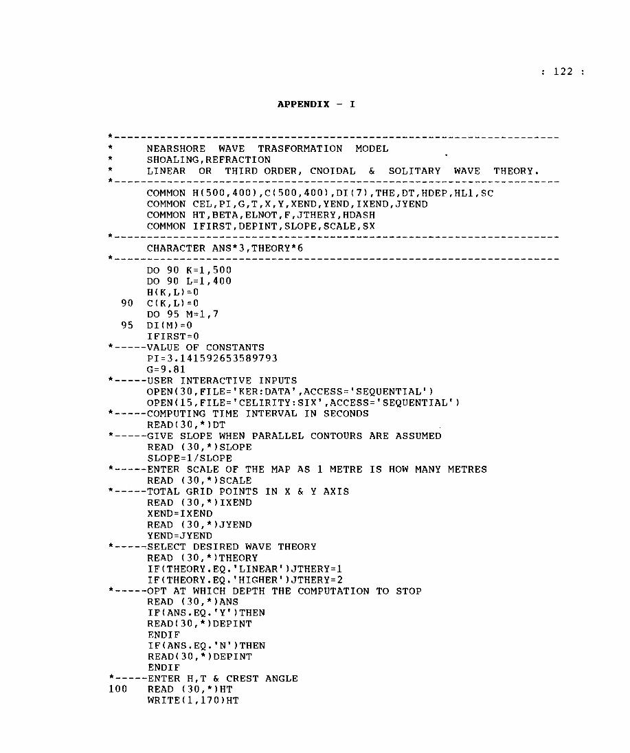
122

APPENDIX - I

*--------------------------------------------------------------------* * *

NEARSHORE WAVE TRASFORMATION MODEL SHOALING,REFRACTION LINEAR OR THIRD ORDER, CNOIDAL & SOLITARY WAVE THEORY.

*--------------------------------------------------------------------COMMON H(500,400),C(500,400),DI(7),THE,DT,HDEP,HL1,SC COMMON CEL,PI,G,T,X,Y,XEND,YEND,IXEND,JYEND COMMON HT,BETA,ELNOT,F,JTHERY,HDASH COMMON IFIRST,DEPINT,SLOPE,SCALE,SX

*--------------------------------------------------------------------CHARACTER ANS*3,THEORY*6

*--------------------------------------------------------------------DO 90 K=1,500 DO 90 L=l, 400 H(K,L)=O

90 C(K,L)=O DO 95 M=1,7

95 DI(M)=O IFIRST=O

*-----VALUE OF CONSTANTS PI=3.141592653589793 G=9.81

*-----USER INTERACTIVE INPUTS OPEN(30,FILE='KER:DATA' ,ACCESS='SEQUENTIAL') OPEN(15,FILE='CELIRITY:SIX' ,ACCESS='SEQUENTIAL')

*-----COMPUTING TIME INTERVAL IN SECONDS READ(30,*)DT

*-----GIVE SLOPE WHEN PARALLEL CONTOURS ARE ASSUMED READ (30,*)SLOPE SLOPE=l/SLOPE

*-----ENTER SCALE OF THE MAP AS 1 METRE IS HOW MANY METRES READ (30,*)SCALE

*--~--TOTAL GRID POINTS IN X & Y AXIS READ (30,*)IXEND XEND=IXEND READ (30,*)JYEND YEND=JYEND

*----~SELECT DESIRED WAVE THEORY READ (30,*)THEORY IF(THEORY.EQ.'LINEAR')JTHERY=l IF(THEORY.EQ.'HIGHER')JTHERY=2

*-----OPT AT WHICH DEPTH THE COMPUTATION TO STOP READ (30,*)ANS IF(ANS.EQ.'Y')THEN READ(30,*)DEPINT ENDIF IF(ANS.EQ.'N')THEN READ(30,*)DEPINT ENDIF

*-----ENTER H,T & CREST ANGLE 100 READ (30,*)HT

WRITE(1,170)HT

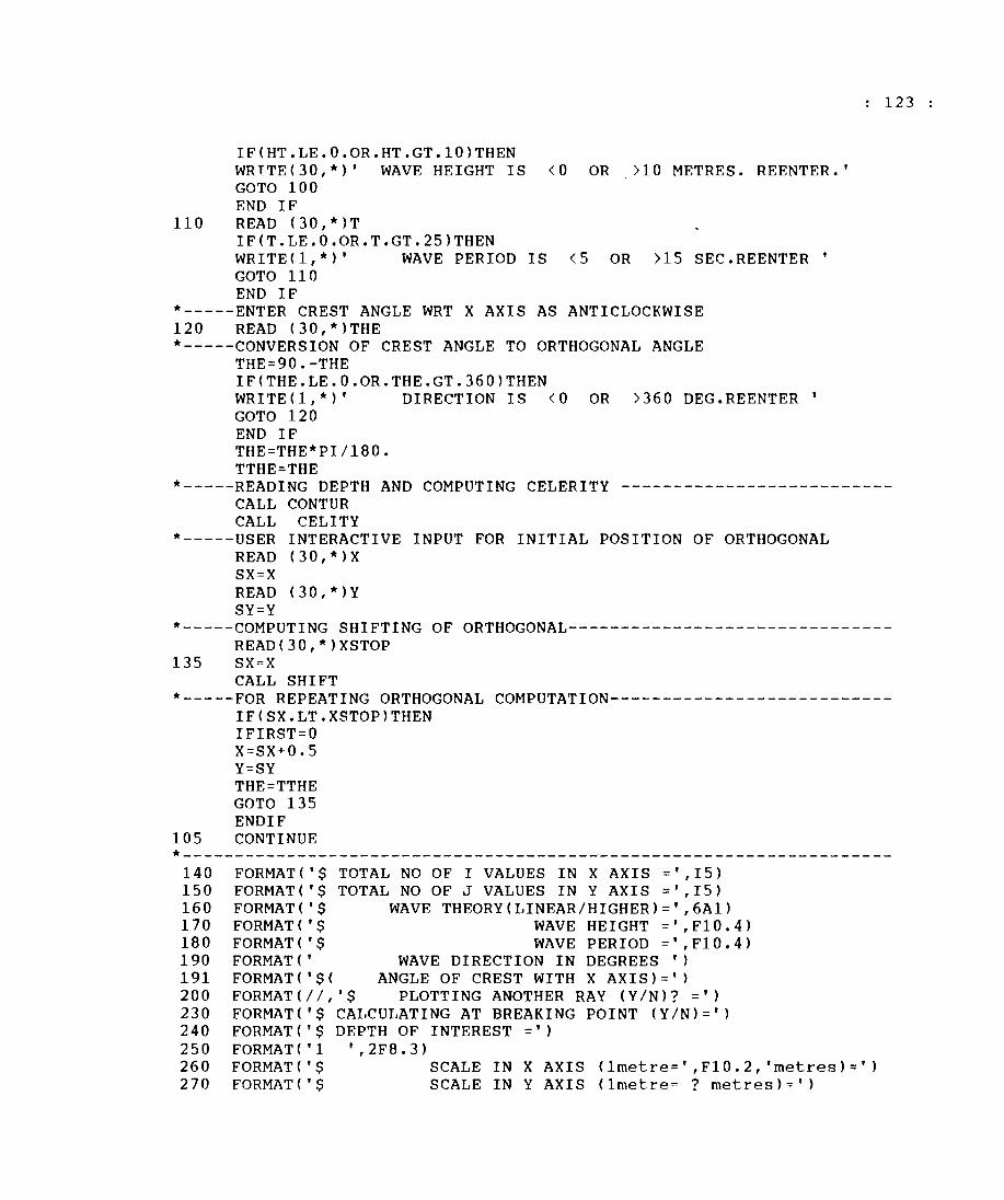
IFCHT.LE.0.OR.HT.GT.10)THEN WRtTEC30,*)' WAVE HEIGHT IS <0 OR >10 METRES. REENTER.' GOTO 100 END IF

110 READ C30,*)T IFCT.LE.0.OR.T.GT.25)THEN WRITECl,*)' WAVE PERIOD IS <5 OR >15 SEC.REENTER ' GOTO 110 END IF

*-----ENTER CREST ANGLE WRT X AXIS AS ANTICLOCKWISE 120 READ C30,*)THE *-----CONVERSION OF CREST ANGLE TO ORTHOGONAL ANGLE

THE=90.-THE IFCTHE.LE.0.OR.THE.GT.360)THEN WRITE(l,*)' DIRECTION IS <0 OR >360 DEG.REENTER ' GOTO 120 END IF THE=THE*PI/180. TTHE=THE

123

*-----READING DEPTH AND COMPUTING CELERITY -------------------------­CALL CONTUR CALL CELITY

*-----USER INTERACTIVE INPUT FOR INITIAL POSITION OF ORTHOGONAL READ (30,*)X SX=X READ C30,*)Y SY=Y

*-----COMPUTING SHIFTING OF ORTHOGONAL------------------------------­READC30,*)XSTOP

135 SX=X CALL SHIFT

*-----FOR REPEATING ORTHOGONAL COMPUTATION--------------------------­IFCSX.LT.XSTOP)THEN IFIRST=O X=SX+0.5 Y=SY THE=TTHE GOTO 135 ENDIF

105 CONTINUE *--------------------------------------------------------------------

140 FORMATC'$ TOTAL NO OF I VALUES IN X AXIS =',15) 150 FORMAT('$ TOTAL NO OF J VALUES IN Y AXIS =',15) 160 FORMAT('$ WAVE THEORYCLINEAR/HIGHER)=',6Al) 170 FORMAT('$ WAVE HEIGHT =',FI0.4) 180 FORMAT('$ WAVE PERIOD =',FI0.4) 190 FORMAT(' WAVE DIRECTION IN DEGREES ') 191 FORMATC'$C ANGLE OF CREST WITH X AXIS)=') 200 FORMAT(II,'$ PLOTTING ANOTHER RAY (Y/N)? =') 230 FORMATC'$ CALCULATING AT BREAKING POINT (Y/N)=') 240 FORMAT('$ DEPTH OF INTEREST =') 250 FORMAT('l ',2F8.3) 260 FORMAT('$ SCALE IN X AXIS Clmetre=',F10.2,'metres)=') 270 FORMATC'$ SCALE IN Y AXIS Clmetre= ? metres)=')

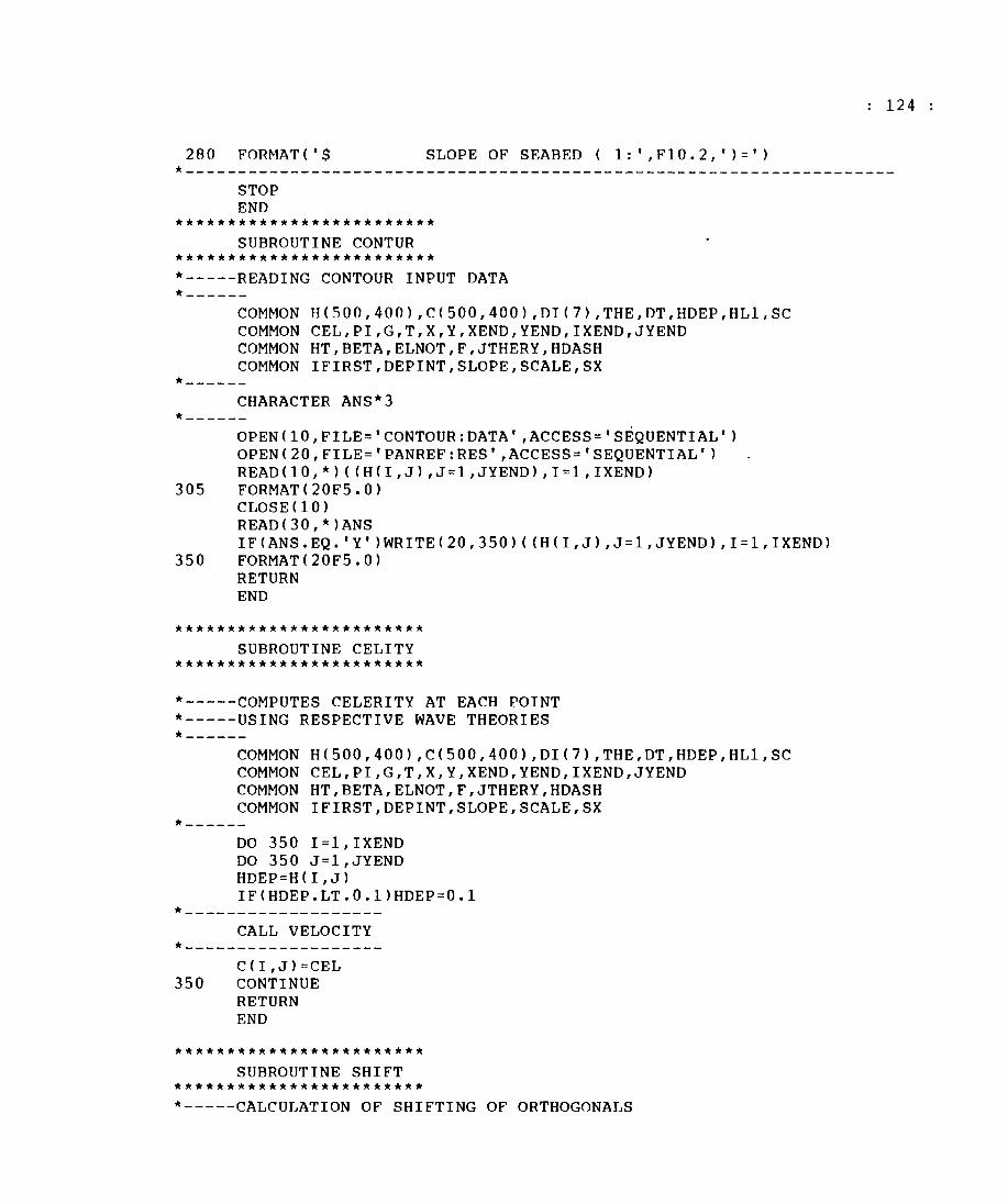
124

280 FORMAT('$ SLOPE OF SEABED ( 1:' ,FI0.2,' )=') *--------------------------------------------------------------------

STOP END

************************* SUBROUTINE CONTUR

************************* *-----READING CONTOUR INPUT DATA *------

COMMON H(500,400),C(500,400),DI(7),THE,DT,HDEP,HLl,SC COMMON CEL,PI,G,T,X,Y,XEND,YEND,IXEND,JYEND COMMON HT,BETA,ELNOT,F,JTHERY,HDASH COMMON IFIRST,DEPINT,SLOPE,SCALE,SX

*------CHARACTER ANS*3

*------OPEN(10,FILE='CONTOUR:DATA' ,ACCESS='SEQUENTIAL') OPEN(20,FILE='PANREF:RES',ACCESS='SEQUENTIAL') READ(10,*)«H(I,J),J=I,JYEND),I=I,IXEND)

305 FORMAT(20F5.0) CLOSE(10) READ(30,*)ANS IF(ANS.EQ.'Y' )WRITE(20,350)«H(I,J),J=1,JYEND),I=I,IXEND)

350 FORMAT(20F5.0) RETURN END

************************ SUBROUTINE CELITY

************************

*-----COMPUTES CELERITY AT EACH POINT *-----USING RESPECTIVE WAVE THEORIES *------

COMMON H(500,400),C(500,400),DI(7),THE,DT,HDEP,HLl,SC COMMON CEL,PI,G,T,X,Y,XEND,YEND,IXEND,JYEND COMMON HT,BETA,ELNOT,F,JTHERY,HDASH COMMON IFIRST,DEPINT,SLOPE,SCALE,SX

*------DO 350 I=I,IXEND DO 350 J=I,JYEND HDEP=H (I, J) IF(HDEP.LT.O.l)HDEP=O.1

*-------------------CALL VELOCITY

*-------------------C (I,J) =CEL

350 CONTINUE RETURN END

************************ SUBROUTINE SHIFT

************************ *-----CALCULATION OF SHIFTING OF ORTHOGONALS

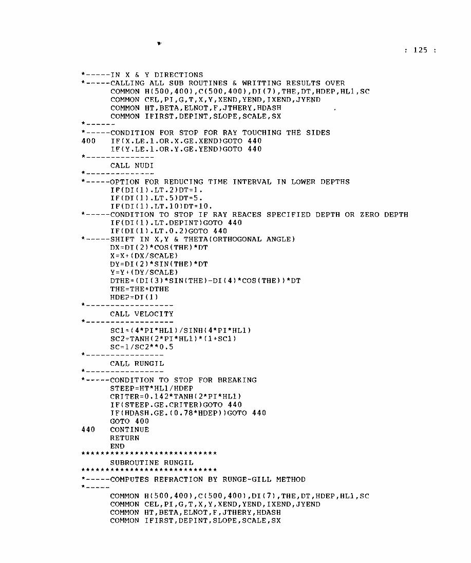
*-----IN X & Y DIRECTIONS *-----CALLING ALL SUB ROUTINES & WRITTING RESULTS OVER

COMMON H(500,400),C(500,400),DI(7),THE,DT,HDEP,HL1,SC COMMON CEL,PI,G,T,X,Y,XEND,YEND,IXEND,JYEND COMMON HT,BETA,ELNOT,F,JTHERY,HDASH COMMON IFIRST,DEPINT,SLOPE,SCALE,SX

*------*-----CONDITION FOR STOP FOR RAY TOUCHING THE SIDES 400 IF(X.LE.1.0R.X.GE.XEND)GOTO 440

IF(Y.LE.1.0R.Y.GE.YEND)GOTO 440 *--------------

CALL NUDI *--------------*-----OPTION FOR REDUCING TIME INTERVAL IN LOWER DEPTHS

IF(DI(1).LT.2)DT=1. IF(DI(1).LT.5)DT=5. IF(DI(1).LT.10)DT=10.

*-----CONDITION TO STOP IF RAY REACES SPECIFIED DEPTH OR ZERO DEPTH IF(DI(l).LT.DEPINT)GOTO 440 IF(DI(1).LT.0.2)GOTO 440

*-----SHIFT IN X,Y & THETA(ORTHOGONAL ANGLE) DX=DI(2)*COS(THE)*DT X=X+(DX/SCALE) DY=DI(2)*SIN(THE)*DT Y=Y+(DY/SCALE) DTHE=(DI(3)*SIN(THE)-DI(4)*COS(THE))*DT THE=THE+DTHE HDE?=DI(l)

*------------------CALL VELOCITY

*------------------SCl=(4*PI*HLl)/SINH(4*PI*HL1) SC2=TANH(2*PI*HLl)*(1+SC1) SC=1/SC2**0.5

*----------------CALL RUNGIL

*----------------*-----CONDITION TO STOP FOR BREAKING

STEEP=HT*HL1/HDEP CRITER=0.142*TANH(2*PI*HLl) IF(STEEP.GE.CRITER)GOTO 440 IF(HDASH.GE.(0.78*HDEP))GOTO 440 GOTO 400

440 CONTINUE RETURN END

**************************** SUBROUTINE RUNGIL

**************************** *-----COMPUTES REFRACTION BY RUNGE-GILL METHOD *-----

COMMON H(500,400),C(500,400),DI(7),THE,DT,HDEP,HLl,SC COMMON CEL,PI,G,T,X,Y,XEND,YEND,IXEND,JYEND COMMON HT,BETA,ELNOT,F,JTHERY,HDASH COMMON IFIRST,DEPINT,SLOPE,SCALE,SX

125

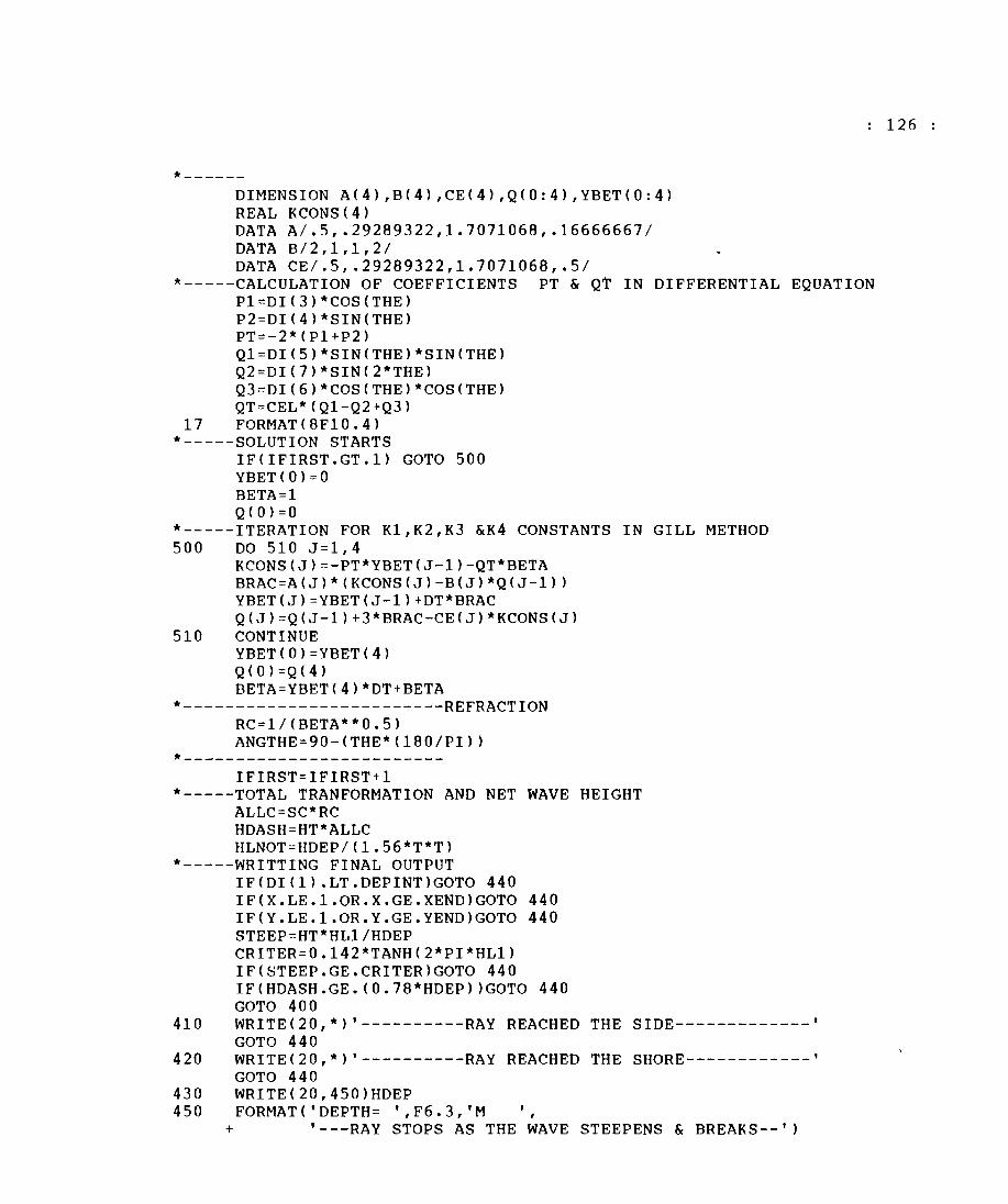
*------DIMENSION A(4),BC4),CEC4),QCO:4),YBETCO:4) REAL KCONS(4) DATA A/.5,.29289322,1.7071068,.166666671 DATA B/2,1,1,21 DATA CE/.5,.29289322,1.7071068,.51

*-----CALCULATION OF COEFFICIENTS PT & QT IN DIFFERENTIAL EQUATION P1=DI(3)*COSCTHE) P2=DI(4)*SINCTHE) PT=-2*CP1+P2) Q1=DI(5)*SIN(THE)*SINCTHE) Q2=DI(7)*SIN(2*THE) Q3=DI(6)*COSCTHE)*COSCTHE) QT=CEL*CQ1-Q2+Q3)

17 FORMATC8F10.4) *-----SOLUTION STARTS

IFCIFIRST.GT.1) GOTO 500 YBETCO)=O BETA=1 QCO)=O

*-----ITERATION FOR K1,K2,K3 &K4 CONSTANTS IN GILL METHOD 500 DO 510 J=1,4

KCONSCJ)=-PT*YBETCJ-1)-QT*BETA BRAC=ACJ)*CKCONSCJ)-B(J)*QCJ-1» YBETCJ)=YBETCJ-1)+DT*BRAC QCJ)=QCJ-1)+3*BRAC-CE(J)*KCONS(J)

510 CONTINUE YBETCO)=YBETC4) QCO)=Q(4) BETA=YBET(4)*DT+BETA

*-------------------------REFRACTION RC=1/(BETA**0.5) ANGTHE=90-CTHE*C180/PI»

*-------------------------IFIRST=IFIRST+1

*-----TOTAL TRANFORMATION AND NET WAVE HEIGHT ALLC=SC*RC HDASH=HT*ALLC HLNOT=HDEP/C1.56*T*T)

*-----WRITTING FINAL OUTPUT IFCDI(1).LT.DEPINT)GOTO 440 IFCX.LE.1.0R.X.GE.XEND)GOTO 440 IFCY.LE.1.0R.Y.GE.YEND)GOTO 440 STEEP=HT*HL1/HDEP CRITER=0.142*TANHC2*PI*HL1) IFCSTEEP.GE.CRITER)GOTO 440 IFCHDASH.GE.CO.78*HDEP»GOTO 440 GOTO 400

410 WRITEC20,*)'----------RAY REACHED THE SIDE-------------' GOTO 440

420 WRITEC20,*)'----------RAY REACHED THE SHORE------------' GOTO 440

430 WRITEC20,450)HDEP 450 FORMAT('DEPTH= ',F6.3,'M ,

+ '---RAY STOPS AS THE WAVE STEEPENS & BREAKS--')

126

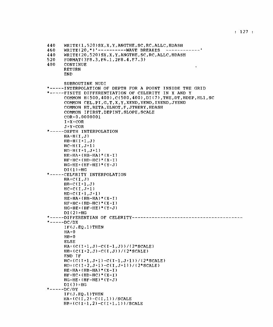
440 WRITEC1,520)SX,X,Y,ANGTHE,SC,RC,ALLC,HDASH 460 WRITEC20,*)'----------WAVE BREAKES ------------440 WRITEC20,520)SX,X,Y,ANGTHE,SC,RC,ALLC,HDASH 520 FORM~TC3F8.3,F6.1,2F8.4,F7.3) 400 CONTINUE

RETURN END

SUBROUTINE NUDI *-----INTERPOLATION OF DEPTH FOR A POINT INSIDE THE GRID *-----FINITE DIFFERENTIATION OF CELERITY IN X AND Y

COMMON HC500,400),CC500,400),DIC7),THE,DT,HDEP,HL1,SC COMMON CEL,PI,G,T,X,Y,XEND,YEND,IXEND,JYEND COMMON HT,BETA,ELNOT,F,JTHERY,HDASH COMMON IFIRST,DEPINT,SLOPE,SCALE COR=0.0000001 I=X+COR J=Y+COR

*-----DEPTH INTERPOLATION HA=HCI,J) HB=H Cl + 1, J) HC=HCl,J+1) HD=HCI+1,J+1) HE=HA+CHB-HA)*CX-I) HF=HC+CHD-HC)*(X-I) HG=HE+CHF-HE)*CY-J) 01 C 1) =HG

*-----CELF.RITY INTERPOLATION HA=CCI,J) HB=C Cl + 1, J) HC=CCl,J+1) HD=CCI+1,J+1) HE=HA+CHB-HA)*CX-I) HF=HC+CHD-HC)*CX-I) HG=HE+CHF-HE)*CY-J) DI(2)=HG

127

*-----DIFFERENTIAN OF CELERITY--------------------------------------­*-----DC/DX

IFCJ.EQ.1)THEN HA=O HB=O ELSE HA=CC(I+1,J)-CCI-1,J»/(2*SCALE) HB=CCCI+2,J)-C(I,J»/C2*SCALE) END IF HC=CC(I+1,J+1)-C(I-1,J+1»/(2*SCALE) HD=CCCI+2,J+1)-CCI,J+1»/C2*SCALE) HE=HA+CHB-HA)*CX-I) HF=HC+CHD-HC)*CX-I) HG=HE+CHF-HE)*CY-J) DI(3)=HG

*-----DC/DY IFCJ.EQ.1)THEN HA=CCCI,2)-C(I,1»/SCALE HB=CCCI+1,2)-CCI+1,1»/SCALE

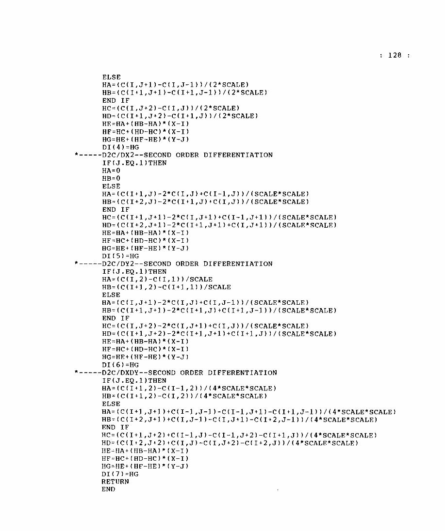
ELSE HA=(C(I,J+1)-C(I,J-1»/(2*SCALE) HB=(C(I+1,J+1)-C(I+1,J-1»/(2*SCALE) END IF HC=(CCI,J+2)-C(I,J»/(2*SCALE) HD=(C(I+1,J+2)-C(I+1,J»/(2*SCALE) HE=HA+(HB-HA)*(X-I) HF=HC+(HD-HC)*(X-I) HG=HE+(HF-HE)*(Y-J) DI(4)=HG

*-----D2C/DX2--SECOND ORDER DIFFERENTIATION IF(J.EQ.1)THEN HA=O HB=O ELSE HA=(C(I+1,J)-2*C(I,J)+C(I-1,J»/(SCALE*SCALE) HB=(CCI+2,J)-2*C(I+1,J)+C(I,J»/(SCALE*SCALE) END IF HC=(C(I+l,J+l)-2*C(I,J+1)+C(I-1,J+l»/(SCALE*SCALE) HD=(C(I+2,J+1)-2*C(I+l,J+l)+C(I,J+l»/(SCALE*SCALE) HE=HA+(HB-HA)*(X-I) HF=HC+CHD-HC)*(X-I) HG=HE+(HF-HE)*CY-J) DI(5)=HG

*-----D2C/DY2--SECOND ORDER DIFFERENTIATION IF(J.EQ.l)THEN HA=CC(I,2)-C(I,1»/SCALE HB=(CCI+l,2)-C(I+1,1»/SCALE ELSE HA=(C(I,J+l)-2*CCI,J)+C(I,J-l»/(SCALE*SCALE) HB=(C(I+l,J+l)-2*C(I+l,J)+CCI+l,J-1»/(SCALE*SCALE) END IF HC=CCCI,J+2)-2*CCI,J+1)+CCI,J»/(SCALE*SCALE) HD=CCCI+l,J+2)-2*C(I+l,J+1)+CCI+1,J»/(SCALE*SCALE) HE=HA+CHB-HA)*(X-I) HF=HC+(HD-HC)*(X-I) HG=HE+CHF-HE)*CY-J) DI(6)=HG

*-----D2C/DXDY--SECOND ORDER DIFFERENTIATION IF(J.EQ.!)THEN HA=CC(I+l,2)-CCI-1,2»/(4*SCALE*SCALE) HB=(C(I+l,2)-CCI,2»/(4*SCALE*SCALE)

128

ELSE HA=CCCI+1,J+l)+C(I-1,J-l)-CCI-1,J+1)-C(I+1,J-1»/C4*SCALE*SCALE) HB=CC(I+2,J+l)+C(I,J-l)-C(I,J+l)-C(I+2,J-1»/(4*SCALE*SCALE) END IF HC=(C(I+l,J+2)+CCI-1,J)-C(I-1,J+2)-CCI+1,J»/(4*SCALE*SCALE) HD=(C(I+2,J+2)+C(I,J)-C(I,J+2)-C(I+2,J»/(4*SCALE*SCALE) HE=HA+(HB-HA)*CX-I) HF=HC+(HD-HC)*CX-I) HG=HE+(HF-HE)*(Y-J) DI(7)=HG RETURN END

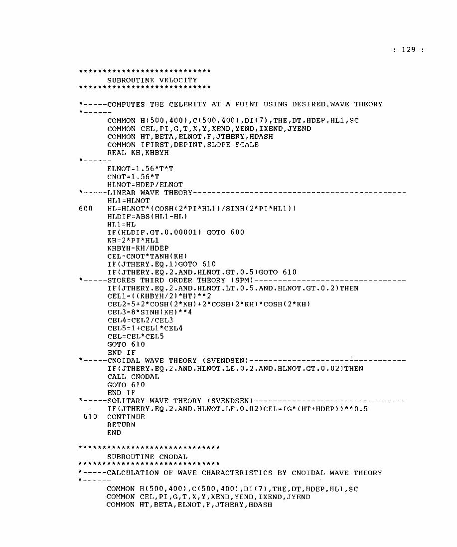
**************************** SUBROUTINE VELOCITY

****************************

*-----COMPUTES THE CELERITY AT A POINT USING DESIRED. WAVE THEORY *------

COMMON H(SOO,400),C(SOO,400),DI(7),THE,DT,HDEP,HL1,SC COMMON CEL,PI,G,T,X,Y,XEND,YEND,IXEND,JYEND COMMON HT,BETA,ELNOT,F,JTHERY,HDASH COMMON IFIRST,DEPINT,SLOPE.SCALE REAL KH,KHBYH

*------ELNOT=1.S6*T*T CNOT=1.56*T HLNOT=HDEP/ELNOT

129

*-----LINEAR WAVE THEORY--------------------------------------------­HL1=HLNOT

600 HL=HLNOT*(COSH(2*PI*HL1)/SINH(2*PI*HL1» HLDIF=ABS(HL1-HL) HL1=HL IF(HLDIF.GT.0.00001) GOTO 600 KH=2*PI*HL1 KHBYH=KH/HDEP CEL=CNOT*TANH(KH) IF(JTHERY.EQ.1)GOTO 610 IF(JTHERY.EQ.2.AND.HLNOT.GT.0.S)GOTO 610

*-----STOKES THIRD ORDER THEORY (SPM)-------------------------------­IF(JTHERY.EQ.2.AND.HLNOT.LT.0.5.AND.HLNOT.GT.0.2)THEN CEL1=«KHBYH/2)*HT)**2 CEL2=5+2*COSH(2*KH)+2*COSH(2*KH)*COSH(2*KH) CEL3=8*SINH(KH)**4 CEL4=CEL2/CEL3 CELS=1+CEL1*CEL4 CEL=CEL*CEL5 GOTO 610 END IF

*-----CNOIDAL WAVE THEORY (SVENDSEN)--------------------------------­IF(JTHERY.EQ.2.AND.HLNOT.LE.0.2.AND.HLNOT.GT.0.02)THEN CALL CNODAL GOTO 610 END IF

*-----SOLITARY WAVE THEORY (SVENDSEN)-------------------------------­IF(JTHERY.EQ.2.AND.HLNOT.LE.0.02)CEL=(G*(HT+HDEP»**0.S

610 CONTINUE RETURN END

****************************** SUBROUTINE CNODAL

****************************** *-----CALCULATION OF WAVE CHARACTERISTICS BY CNOIDAL WAVE THEORY *------

COMMON H(SOO,400),C(SOO,400),DI(7),THE,DT,HDEP,HL1,SC COMMON CEL,PI,G,T,X,Y,XEND,YEND,IXEND,JYEND COMMON HT,BETA,ELNOT,F,JTHERY,HDASH

COMMON IFIRST,DEPINT,SLOPE,SCALE *------

DIMENSION ELH(0:4,17) DATA «ELH(I,J),I=0,4),J=1,17)1

+6.7,6.8,7.1,7.6,8.2,9.2,9.3,9.8,10.4,11.2, +11.4,11.6,12.3,13.1,14,13.5,13.9,14.7,15.7,16.7, +15.6,16.1,17.1,18.3,19.5,17.6,18.3,19.5,20.9,22.2, +19.7,20.5,21.9,23.4,24.9,21.7,22.7,24.3,26,27.6, +23.7,24.9,26.7,28.5,30.3,25.7,27.1,29.1,31.1,33, +27.8,29.3,31.4,33.6,35.7,29.8,31.5,33.8,36.1,38.4, +31.8,33.7,36.2,38.7,41.1,33.8,35.9,38.6,41.2,43.8, +35.8,38.1,40.9,43.8,46.5,37.8,40.3,43.3,46.3,49.2, +39.9,42.5,45.7,48.8,51.91

*------HTH=HT/HDEP TGH=T*«G/HDEP)**0.5) IF(HTH.GT.0.8.0R.TGH.LT.8.0R.TGH.GT.40)GOTO 700 XX=HTH/O.2 YY=(TGH/2)-3 I=XX J=YY HA=ELH(I,J) HB=ELH(I+l,J) HC=ELH(I,J+1) HD=ELH(I+1,J+1) HE=HA+(HB-HA)*(XX-I) HF=HC+(HD-HC)*(XX-I) HG=HC+(HF-HE)*(YY-J) ELBYH=HG HL1=1/ELBYH CEL=ELBYH*HDEP/T

700 CONTINUE RETURN END

- G' Cj'305 ----

130