2016 IEEE INTERNATIONAL WORKSHOP ON MACHINE LEARNING FOR SIGNAL PROCESSING, SEPT. 13–16, 2016, SALERNO, ITALY

BDL.NET: BAYESIAN DICTIONARY LEARNING IN INFER.NET

Tom Diethe, Niall Twomey, Peter Flach

Intelligent Systems Laboratory, University of Bristol, UK

ABSTRACT

We introduce and analyse a flexible and efficient implemen-tation of Bayesian dictionary learning for sparse coding. Byplacing Gaussian-inverse-Gamma hierarchical priors on thecoefficients, the model can automatically determine the re-quired sparsity level for good reconstructions, whilst also au-tomatically learning the noise level in the data, obviating theneed for heuristic methods for choosing sparsity levels. Thismodel can be solved efficiently using Variational MessagePassing (VMP), which we have implemented in the Infer.NETframework for probabilistic programming and inference. Weanalyse the properties of the model via empirical validationon several accelerometer datasets. We provide source code toreplicate all of the experiments in this paper.

Index Terms— Sparse Coding, Dictionary Learning,Bayesian, Accelerometers

1. INTRODUCTION

Our motivating application is Activity Recognition (AR),which is usually performed for the purposes of understand-ing the Activities of Daily Living (ADL) of a given indi-vidual. One of the most popular methods for the study ofADL is through the use of a wearable device containing anaccelerometer, often combined with gyroscopes, which mea-sure the degree of rotation as the device rotates in any its axes.Since gyroscopes consume several orders of magnitude morepower than low power accelerometers, we are most interestedin accelerometers only.

Traditional methods for classification of accelerometersignals involve computing features in both the temporal andfrequency domains over a temporal window - see e.g. [1].One effect of this is to reduce the temporal dependence ofneighbouring examples, which enables the use of standardclassification algorithms. There is a trade-off here: longerwindows mean less dependence and less computational bur-den; however in extremis, the probability that a given windowinvolves only a single activity class diminishes. We are there-fore interested in a compact representation of the signals, that

The SPHERE Interdisciplinary Research Collaboration is funded by theUK Engineering and Physical Sciences Research Council (EPSRC) underGrant EP/K031910/1.

also contains the necessary information to be discriminatorybetween activity classes.

1.1. Dictionary Learning

Dictionary Learning, also known as Sparse Coding [2] isa class of unsupervised methods for learning sets of over-complete bases to represent data in a parsimonious manner.The aim of sparse coding is to find a set of vectors di, knownas a dictionary, such that we can represent an input vectorx 2 Rn as a linear combination of these vectors:

x =kX

i=1

zidi s.t. k � n. (1)

While there exist efficient techniques to learn a complete setof vectors (i.e. a basis) such as Principal Component Analy-sis (PCA)[3], an over-completeness can achieve a more sta-ble, robust, and compact decomposition than using a basis[4]. However, with an over-complete basis, the coefficientszi are no longer uniquely determined by the input vector x.Therefore, in sparse coding, we introduce additional spar-sity constraints to resolve the degeneracy introduced by over-completeness.

Sparsity is defined as having few non-zero componentszi or many that are close to zero. The sparse coding costfunction on a set of m input vectors arranged in the columnsof the matrix X 2 Rn⇥m as

minZ,D

kX�DZk2F + �nX

i=1

⌦(zi)

s.t. kdik2 C, 8i = 1, . . . , k.

where D 2 Rn⇥k is the set of basis vectors (dictionary),Z 2 Rk⇥n is the set of coefficients for each example, and ⌦(.)is a sparsity inducing regularisation function, and the scalingconstant � determines the relative importance of good recon-structions and sparsity. The most direct measure of sparsityis the L0 quasi-norm ⌦(zi) = 1(|zi| > 0), but it is non-differentiable and difficult to optimise in general. A commonchoice for the sparsity cost ⌦(.) is the L1 penalty ⌦(zi) =Pn

i=1 |zi| (see [5] for a review). Since it is also possible tomake the sparsity penalty arbitrarily small by scaling down zi

978-1-5090-0746-2/16/$31.00 ©2016 Crown

and scaling di up by some large constant, kdk2 is constrainedto be less than some constant C.

Since the optimisation problem is not jointly convex in Zand D, sparse coding consists of performing two separate op-timisations: (1) over coefficients zi for each training examplexi with D fixed; and (2) over basis vectors D across the wholetraining set with Z fixed. Using an L1 sparsity penalty, sub-problem (1) reduces to solving an L1 regularised least squaresproblem which is convex in zi which can be solved using stan-dard convex optimisation software such as CVX [6]. With adifferentiable ⌦(·) such as the log penalty, conjugate gradientmethods can also be used. Sub-problem (2) reduces to a leastsquares problem with quadratic constraints which is convexin d, for which again there are standard methods available.

1.2. Online Dictionary Learning

As described thus far, dictionary learning algorithms requirethe entire set of training signals X, which puts a limitation onthe sizes of problems that can be tackled, and means that theycannot operate in an online streaming scenario. An onlineversion of dictionary learning was introduced by [7], whichinvolved iteratively finding the sparse representation for eachdata point xi as it arrives, and then updating D using a block-coordinate approach.

1.3. Our Contributions

• We improve on existing methods for Bayesian DictionaryLearning (BDL), with a more stable model • We give anefficient implementation using deterministic approximations• We show that priors that do not enforce sparsity can stillresult in sparse representations, whilst giving better recon-structions • We demonstrate how such models can be appliedto accelerometer signals

2. RELATED WORK

A Bayesian approach to the dictionary learning problem ishighly appealing for several reasons. Firstly, it is possible tolearn the noise level directly from the data, rather than havingto specify it or estimate using crude heuristics. Secondly, itallows us to consider building larger models, such as hierar-chical models that enable us to reason about the differencesbetween individuals and groups of people, and also to con-sider transfer learning.

A hierarchical Bayesian model for dictionary learningwas first introduced by [8], in which a Gaussian-inverseGamma hierarchical prior was used to promote the sparsityof the representation. The authors argued that better learningwas achieved compared to baselines in the case where thereis a limited number of training signals. We will discuss therelation to our work in section 3.

An appealing nonparametric Bayesian approach to theproblem was introduced by [9], which allows an adapted dic-tionary size using an Indian Buffet Process prior. Currently,however, there are no efficient methods for inference in thisclass of models, which somewhat limits their use.

In terms of the application area of interest here, featurelearning was applied to AR from accelerometer data by [10],where the authors investigated amongst other things PCA andauto-encoder networks. Dictionary learning would be a nat-ural extension here. Following on from this, a form of shiftinvariant sparse coding was proposed for the same task by[11]. The authors use an approach that can be seen as a formof convolutional sparse coding, with promising classificationperformance.

3. METHODS

We first give a generative model for eq. (1), in which we positthat our signals are generated by the same linear combinationof bases, and give parametric forms for the (latent) variablesand include a noise model.

X = DZ+N,

p(D) =nY

i=1

kY

j=1

N (di,j ;↵i,j ,��1),

p(↵) =nY

i=1

kY

j=1

N (↵i,j ; 0, 1),

p(�) =nY

i=1

kY

j=1

Ga(�i,j ; 1, 1),

p(Z|⌧ ) =kY

i=1

mY

j=1

N (zi,j ; 0, ⌧�1i,j ),

p(⌧ ) =kY

i=1

mY

j=1

Ga(⌧i,j ; a, b),

p(N) =nY

i=1

mY

j=1

N (n; 0,�)

p(�) = Ga(�; a, b), (2)

where N is the Gaussian distribution for a given mean andvariance and Ga is the Gamma distribution for a given shapeand rate.

This model builds on that of [8], and is shown in fig. 1.There are several key differences. Firstly, rather than using afixed value for �, which defines the precision of the dictionaryatoms, we instead put a Gamma prior over �, which allows thedictionary atoms to be automatically scaled. In their experi-ments, Yang et. al. used a value of � = 1 when using Gibbssampling, and a value of � = 10�8 when using VariationalInference. It is not clear why they had to make this decision,

x

N

dot

d z

↵ �0

⌧

�

a b

N N

Ga(1, 1)

GaN (0, 1) Ga(1, 1)

n m

k

Fig. 1: Factor graph representing a hierarchical Bayesianmodel for dictionary learning.

but our experiments show that the additional Gamma prior ap-pears to obviate the need to do this. Furthermore, we place anadditional level of hierarchy through the variables ↵ on themeans of the dictionary components, which can aid onlinelearning.

3.1. Inference

In this work, we employ Variational Message Passing (VMP),which is an efficient deterministic approximation algorithmfor applying variational inference to Bayesian graphical mod-els [12]. Like Belief Propagation (BP) and Expectation Prop-agation (EP) [13], VMP proceeds by sending messages be-tween nodes in the network and updating posterior beliefs us-ing local operations at each node. Each such update increasesa lower bound on the log evidence at that node, (unless al-ready at a local maximum). VMP can be applied to a verygeneral class of conjugate-exponential models because it usesa factorised variational approximation, and by introducing ad-ditional variational parameters, VMP can be applied to mod-els containing non-conjugate distributions. The VMP frame-work also allows the lower bound to be evaluated, which canbe used both for model comparison and for detection of con-vergence.

To break symmetry, we randomly initialise the dictionaryelements to independently and identically distributed (IID)draws from a standard normal distribution. For consistency,we use the same random seed for all experiments.

4. EXPERIMENTS

4.1. Data Sets

HAD dataset [1]

This involved 30 participants aged 19-48 years and six activ-ities were recorded. Each participant wore a smart-phone on

the waist, with tri-axial linear acceleration and tri-axial angu-lar velocity capture using its embedded accelerometer and gy-roscope at a constant rate of 50 Hz. Annotation was done us-ing video-recordings. Each sequence is on average 7 minuteslong. The activities performed were: 1. Walking 2. Ascend-ing stairs 3. Descending stairs 4. Sitting 5. Standing 6. Lyingdown.

SPHERE challenge dataset [14]

This dataset has been collected by our research group in oursmart home deployment and made public as a challenge1. Thetask is prediction of posture and ambulation of participantswho wore a tri-axial accelerometer on the dominant wrist.The accelerometers record data at 20 Hz, with a range of ±8g. Here we examine a subset of the labels available in thedataset that are also found in the HAD dataset, i.e. : 1. Lie2. Stand 3. Walk

4.2. Data pre-processing

The signal streams were split into windows of 3 seconds inlength, from which we computed the magnitude of the ac-celeration vector and subtracted 1 (gravitational force). Thewindowed signals were then normalised to have unit `2-norm

In our comparisons with non-Bayesian sparse coding, weused the SPArse Modeling Software (SPAMS) toolbox 2, andin particular we used the online dictionary learning methoddescribed in [7].

We follow [7] and used the regularisation parameter � =1.2/

pm in all of our experiments (⇡ 0.1 for HAD and ⇡

0.03 for SPHERE). The 1/pm term is a classical normalisa-

tion factor, and the constant 1.2 was shown to yield about 10nonzero coefficients in their experiments.

The methods described here were all implemented usingInfer.NET [15], which is a framework for running Bayesianinference in graphical models, and provides a rich modellinglanguage for a wide variety of applications. In our experi-ments we compile and run the code using Mono3, an opensource implementation of Microsoft’s .NET, running on OS-X and Linux.

4.3. Reconstruction

In order to test reconstruction, in all cases we take the dic-tionary learnt on the training set (2D Gaussian arrays in theBayesian methods), and first compute coefficients for the testsignals using this dictionary. We then reconstruct the signalsusing the trained dictionary and inferred coefficients.

For the performance metric for the quality of reconstruc-tions we will adopt the commonly used root-mean-square er-ror (RMSE) =

pPnt=1(xt � xt)2/n.

1http://irc-sphere.ac.uk/sphere-challenge/home

2http://spams-devel.gforge.inria.fr/

3http://www.mono-project.com/

5. RESULTS AND DISCUSSION

5.1. Convergence of VMP

Before continuing we will first analyse the convergence prop-erties of VMP for the models defined herein. VMP is adeterministic approximation algorithm, and for well-behavedproblems the model evidence (or marginal likelihood) willalways increase and will converge to a local maximum. Wefollow [12], and define convergence by evaluating the modelevidence in the variational posterior after each full round ofmessage passing, checking that the value of the bound doesnot decrease by more than some tolerance. We will refer tothis as “iterative model comparison” (IMC) henceforth.

(a) Convergence of model evidence.

(b) Convergence of hold-out reconstruction error.

Fig. 2: Convergence plots of marginal likelihood and recon-struction error.

In figs. 2a and 2b we have plotted the convergence of themodel evidence on a subset of the HAD dataset and the re-construction error on a hold-out test set respectively. Here weused 1000 instances for training, and computed the RMSE on200 instances from the test set. In order to do so, we had touse a convergence criterion for the inference of test set coeffi-cients and reconstructed signals, for which we used IMC witha tolerance of 10�4. We let the message passing run for 20iterations even if it would have passed the IMC criterion. Itis interesting to note that while the evidence for each of themodels follows similar convergence paths, the reconstructionerrors are clearly in favour of the non-sparse model.

For all further experiments we used the IMC method witha tolerance of 10�3 for dictionary learning, coefficient esti-mation, and reconstruction.

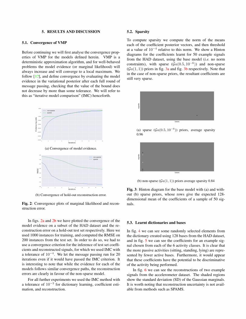
5.2. Sparsity

To compute sparsity we compute the norm of the meanseach of the coefficient posterior vectors, and then thresholdat a value of 10�4 relative to this norm. We show a Hintondiagrams for the coefficients learnt for 50 example signalsfrom the HAD dataset, using the base model (i.e. no normconstraints), with sparse (Ga(0.5, 10�6)) and non-sparse(Ga(1, 1)) priors in fig. 3a and fig. 3b respectively. Note thatin the case of non-sparse priors, the resultant coefficients arestill very sparse.

(a) sparse (Ga(0.5, 10�6)) priors, average sparsity0.96

(b) non-sparse (Ga(1, 1)) priors average sparsity 0.84

Fig. 3: Hinton diagram for the base model with (a) and with-out (b) sparse priors, whose rows give the expected 128-dimensional mean of the coefficients of a sample of 50 sig-nals.

5.3. Learnt dictionaries and bases

In fig. 4 we can see some randomly selected elements fromthe dictionary created using 128 bases from the HAD dataset,and in fig. 5 we can see the coefficients for an example sig-nal chosen from each of the 6 activity classes. It is clear thatthe more passive activities (sitting, standing, lying) are repre-sented by fewer active bases. Furthermore, it would appearthat these coefficients have the potential to be discriminativeof the activity being performed.

In fig. 6 we can see the reconstructions of two examplesignals from the accelerometer dataset. The shaded regionsshow the standard deviation (SD) of the Gaussian marginals.It is worth noting that reconstruction uncertainty is not avail-able from methods such as SPAMS.

Fig. 4: 16 example bases from the dictionary of 128 basesinferred by BDL using the non-sparse priors.

Fig. 5: Coefficients from accelerometer signals from each ofthe 6 activity classes using 128 bases inferred by BDL usingthe non-sparse priors.

In table 1 we can see a comparison of average reconstruc-tion error and sparsity of BDL with SPAMS on dataset 1. Inalmost all cases, the reconstruction produced by BDL are su-perior to those by SPAMS, whilst achieving comparable spar-sity, even when non-sparse priors are used. The sparsity en-forcing priors do indeed result in sparser solutions, but at thecost of reconstruction error, up until we use 512 bases, atwhich the over-completeness justifies the use of sparsity in-ducing priors.

Table 1: Average test set reconstruction error and sparsity ondataset 1.

SPAMS BDL Sparse BDL

Bases RMSE Sparsity RMSE Sparsity RMSE Sparsity64 0.0480 0.71 0.0519 0.88 0.0293 0.62128 0.0457 0.84 0.0400 0.94 0.0276 0.84256 0.0438 0.92 0.0316 0.99 0.0288 0.93512 0.0423 0.96 0.0224 0.99 0.0231 0.96

Fig. 6: Reconstructions of two example accelerometer sig-nals using 128 bases inferred by BDL using the non-sparsepriors. The original signal is shown in blue, with the recon-structions shown in blue with ± one standard deviation shownas a shaded region.

5.4. Activity Recognition

Here we present results on the use of the computed coeffi-cients as features in a classification algorithm for the purposesof AR on the HAD and SPHERE datasets. Do to space limita-tions, the results presented here should be regarded as a proofof concept. As such, we will not present extensive compar-isons with other feature generation methods or classificationmodels.

We employ the multi-class Bayes Point Machine (BPM)[16], which is a linear Bayesian model for classification, andis also implemented in Infer.NET. Here we will use the max-imum a-posteriori estimates of the coefficient means gener-ated using 64 bases, to which we add a bias feature to givea 65-dimensional feature vector for the classifier. The metricof performance is the per-class one-versus-rest area under theReceiver Operating Characteristic (ROC) curve.

Table 2: Classification results on the HAD dataset. The val-ues given are the per-class area under the ROC curve.

Activity BDL sparse BDL SPAMS

Walking 0.73 0.83 0.88Ascending stairs 0.63 0.60 0.83Descending stairs 0.61 0.34 0.82Sitting 0.74 0.72 0.89Standing 0.51 0.43 0.98Lying down 0.95 0.95 0.95

Average 0.70 0.65 0.89

The results are presented in tables 2 and 3 for the HADand SPHERE datasets respectively. We note that whilst theclassification performance of BDL on HAD is acceptable, itis markedly better for SPAMS. It would appear that despitethe better reconstruction performance of BDL, the bases es-

Table 3: Classification results on the SPHERE dataset. Thevalues given are the per-class area under the ROC curve.

Activity BDL sparse BDL SPAMS

Walking 0.55 0.51 0.46Standing 0.69 0.62 0.44Lying down 0.86 0.85 0.46Average 0.70 0.66 0.45

timated by SPAMS are more discriminative. However on theSPHERE dataset this trend is reversed. Wider empirical vali-dation is required to fully understand these results.

6. CONCLUSIONS AND FURTHER WORK

We have presented a model that is an improvement on existingmethods for Bayesian Dictionary Learning, and have given anefficient implementation using Variational Message Passing.We have shown that even in the over-complete settings, priorsthat do not explicitly enforce sparsity can still result in sparserepresentations, whilst giving better reconstructions. We haveshown how such models can be applied to accelerometer sig-nals, both for reconstruction, and for Activity Recognition,although it is also clear that this is a powerful approach thatcan be applied to a wide range of signals.

There are many possible avenues for further work. Withregards to the accelerometer data itself, as it stands we havenot accounted for the orientation of the device, which in gen-eral is not knowable directly from the accelerometer signalalone. There are heuristic methods to estimate the optimisa-tion, but it would be desirable to integrate this directly intothe model.

As seen above, the current pipeline would involve usingthe maximum a-posteriori estimates of the coefficient meansas features in a classifier. it is conceivable however, to con-struct a model that incorporates both the dictionary learningand classification, in a similar fashion to the (non-Bayesian)approach of [17]. The resultant model should be able to learnbases that are simultaneously useful for reconstruction andclassification.

It would be interesting to explore non-parametric ap-proaches, such as [9], as long as the efficiency that is theresult of using deterministic approximations (such as VMP),and graceful degradation with noisy or corrupted signals isretained.

Finally, it would be interesting to see if the frameworkcan be adapted to perform Convolutional sparse coding akinto [18], for example by setting up a Toeplitz structure withinthe graphical model.

Source code to reproduce all of the experiments in thispaper is provided at: https://github.com/IRC-SPHERE/

bayesian-dictionary-learning.

7. REFERENCES

[1] D Anguita, A Ghio, L Oneto, X Parra, and JL Reyes-Ortiz, “A publicdomain dataset for human activity recognition using smartphones,” inESANN, 2013.

[2] Bruno A Olshausen et al., “Emergence of simple-cell receptive fieldproperties by learning a sparse code for natural images,” Nature, vol.381, no. 6583, pp. 607–609, 1996.

[3] Lindsay I Smith, “A tutorial on principal components analysis,” CornellUniversity, USA, vol. 51, no. 52, pp. 65, 2002.

[4] Radu Balan, Peter G Casazza, Christopher Heil, and Zeph Landau,“Density, overcompleteness, and localization of frames. i. theory,”Journal of Fourier Analysis and Applications, vol. 12, no. 2, pp. 105–143, 2006.

[5] Francis Bach, Rodolphe Jenatton, Julien Mairal, and GuillaumeObozinski, “Optimization with sparsity-inducing penalties,” Foun-dations and Trends® in Machine Learning, vol. 4, no. 1, pp. 1–106,2012.

[6] Michael Grant and Stephen Boyd, “CVX: Matlab software for dis-ciplined convex programming, version 2.1,” http://cvxr.com/

cvx, Mar. 2014.[7] Julien Mairal, Francis Bach, Jean Ponce, and Guillermo Sapiro, “On-

line learning for matrix factorization and sparse coding,” The Journalof Machine Learning Research, vol. 11, pp. 19–60, 2010.

[8] Linxiao Yang, Jun Fang, Hong Cheng, and Hongbin Li, “SparseBayesian dictionary learning with a Gaussian hierarchical model,”CoRR, vol. abs/1503.02144, 2015.

[9] Hong Phuong Dang and Pierre Chainais, “A Bayesian non paramet-ric approach to learn dictionaries with adapted numbers of atoms,” inMachine Learning for Signal Processing (MLSP), 2015 IEEE 25th In-ternational Workshop on. IEEE, 2015, pp. 1–6.

[10] T. Plotz, N.Y. Hammerla, and P. Olivier, “Feature learning for activityrecognition in ubiquitous computing,” in Proc. of the 22nd Int. JointConf. on Artificial Intell. (IJCAI), Toby Walsh, Ed. 2011, pp. 1729–1734, IJCAI/AAAI.

[11] Christian Vollmer, Horst-Michael Gross, and JulianP. Eggert, “Learn-ing features for activity recognition with shift-invariant sparse coding,”in Artificial Neural Networks and Machine Learning ICANN 2013, vol.8131 of Lecture Notes in Computer Science, pp. 367–374. SpringerBerlin Heidelberg, 2013.

[12] John M Winn and Christopher M Bishop, “Variational message pass-ing,” in Journal of Machine Learning Research, 2005, pp. 661–694.

[13] Thomas P Minka, “Expectation propagation for approximate Bayesianinference,” in Proceedings of the Seventeenth conference on Un-certainty in artificial intelligence. Morgan Kaufmann Publishers Inc.,2001, pp. 362–369.

[14] Niall Twomey, Tom Diethe, Meelis Kull, Hao Song, Massimo Cam-plani, Sion Hannuna, Xenofon Fafoutis, Ni Zhu, Pete Woznowski, PeterFlach, and Ian Craddock, “The sphere challenge: Activity recognitionwith multimodal sensor data,” arXiv preprint arXiv:1603.00797, 2016.

[15] T. Minka, J.M. Winn, J.P. Guiver, S. Webster, Y. Zaykov, B. Yangel,A. Spengler, and J. Bronskill, “Infer.NET 2.6,” 2014, Microsoft Re-search Cambridge. http://research.microsoft.com/infernet.

[16] Ralf Herbrich, Thore Graepel, and Colin Campbell, “Bayes point ma-chines,” Journal of Machine Learning Research, vol. 1, pp. 245–279,January 2001.

[17] Julien Mairal, Jean Ponce, Guillermo Sapiro, Andrew Zisserman, andFrancis R. Bach, “Supervised dictionary learning,” in Advances inNeural Information Processing Systems 21, D. Koller, D. Schuurmans,Y. Bengio, and L. Bottou, Eds., pp. 1033–1040. Curran Associates, Inc.,2009.

[18] Hilton Bristow, Anders Eriksson, and Simon Lucey, “Fast convolu-tional sparse coding,” in Computer Vision and Pattern Recognition(CVPR), 2013 IEEE Conference on. IEEE, 2013, pp. 391–398.

View publication statsView publication stats