bcs theory of superconductivity - katzgraber

OutlinesCooper-PairsBCS Theory

Finite Temperatures

BCS Theory of Superconductivity

Thomas BurgenerSupervisor: Dr. Christian Iniotakis

Proseminar in Theoretical PhysicsInstitut fur theoretische Physik

ETH Zurich

June 11, 2007

1 / 52


Finite Temperatures

What is BCS Theory?

Original publication: Phys. Rev. 108, 1175 (1957)

2 / 52


Finite Temperatures

What is BCS Theory?

First “working” microscopic theory for superconductors.

It’s a mean-field theory.

In it’s original form only applied for conventionalsuperconductors.

3 / 52


Finite Temperatures

Outline

1 Cooper-PairsFormation of PairsOrigin of Attractive Interaction

2 BCS TheoryThe model HamiltonianBogoliubov-Valatin-TransformationCalculation of the condensation energy

3 Finite TemperaturesExcitation Energies and the Energy GapDetermination of Tc

Temperature dependence of the energy gapThermodynamic quantities

4 / 52


Finite Temperatures

Formation of PairsOrigin of Attractive Interaction

Outline





5 / 52


Finite Temperatures


Formation of Pairs

Let’s assume the following things:

Consider a material with a filled Fermi sea at T = 0.

Add two more electrons that

interact attractively with each other butdon’t interact with the other electrons except viaPauli-prinziple.

6 / 52


Finite Temperatures


Formation of Pairs

Look for the groundstate wavefunction for the two added electrons,which has zero momentum:

Ψ0(r1, r2) =∑k

(gke

ik·r1e−ik·r2)

(|↑↓〉 − |↓↑〉)

The total wavefunction has to be antisymmetric with respect toexchange of the two electrons. The spin part is antisymmetric andtherefore the spacial part has to be symmetric.

⇒ gk!= g−k.

7 / 52


Finite Temperatures


Formation of Pairs

Inserting this into the Schrodinger equation of the problem leads tothe following equation for the determination of the coefficients gk

and the energy eigenvalue E :

(E − 2εk)gk =∑k>kF

Vkk′gk′ ,

where

Vkk′ =1

Ω

∫V (r)e i(k′−k)·rdr

(r: distance between the two electrons, Ω: normalization volume,εk: unperturbated plane-wave energies).

8 / 52


Finite Temperatures


Formation of Pairs

Since it is hard to analyze the situation for general Vkk′ , assume:

Vkk′ =

−V , EF < εk < EF + ~ωc

0 , otherwise

with ~ωc a cutoff energy away from EF .

9 / 52


Finite Temperatures


Formation of Pairs

With this approximation we get:

1

V=

∑k>kF

1

2εk − E= N(0)

∫ EF +~ωc

EF

dε

2ε− E

=1

2N(0) ln

(2EF − E + 2~ωc

2EF − E

).

If N(0)V 1, we can solve approximativly for the energy E

E ≈ 2EF − 2~ωce− 2

N(0)V < 2EF .

10 / 52


Finite Temperatures


Origin of Attractive Interaction

Negative terms come in when one takes the motion of the ioncores into account, e.g. considering electron-phonon interactions.The physical idea is that

the first electron polarizes the medium by attracting positiveions;

these excess positive ions in turn attract the second electron,giving an effective attractive interaction between the electrons.

11 / 52


Finite Temperatures

The model HamiltonianBogoliubov-Valatin-TransformationCalculation of the condensation energy

Outline





12 / 52


Finite Temperatures


BCS Theory

Having seen that the Fermi sea is unstable against the formation ofa bound Cooper pair when the net interaction is attractive, wemust then expect pairs to condense until an equilibrium point isreached.We need a smart way to write down antisymmetric wavefunctionsfor many electrons. This will be done in the language of secondquantization.

13 / 52


Finite Temperatures


BCS Theory

Introduce the creation operator c†kσ, which creates an electron ofmomentum k and spin σ, and the correspondig annihilationoperator ckσ. These operators obey the standard anticommutationrelations for fermions:

ckσ, c†k′σ′ ≡ ckσc†k′σ′ + c†k′σ′ckσ = δkk′δσσ′

ckσ, ck′σ′ = 0 = c†kσ, c†k′σ′.

Additionally the particle number operator nkσ is defined by

nkσ ≡ c†kσckσ.

14 / 52


Finite Temperatures


The model Hamiltonian

We start with the so-called

pairing-hamiltonian

H =∑kσ

εknkσ +∑kl

Vklc†k↑c

†−k↓c−l↓cl↑,

presuming that it includes the terms that are decisive forsuperconductivity, although it omits many other terms whichinvolve electrons not paired as (k ↑,−k ↓).

15 / 52


Finite Temperatures


The model Hamiltonian

We then add a term −µN , where µ is the chemical potential,leading to

H− µN =∑kσ

ξknkσ +∑kl

Vklc†k↑c

†−k↓c−l↓cl↑.

The inclusion of this factor is mathematically equivalent to takingthe zero of kinetic energy to be at µ (or EF ).

16 / 52


Finite Temperatures


Bogoliubov-Valatin-Transformation

Define:

bk ≡ 〈c−k↓ck↑〉

Because of the large number of particles involved, the fluctuationsof c−k↓ck↑ about these expectations values bk should be small.Therefor express such products of operators formally as

c−k↓ck↑ = bk + (c−k↓ck↑ − bk)

and neglect quantities which are bilinear in the presumably smallfluctuation term in parentheses.

17 / 52


Finite Temperatures



Inserting this in our pairing Hamiltonian we obtain the so-called

model-hamiltonian

HM − µN =∑kσ

ξkc†kσckσ +

∑kl

Vkl(c†k↑c

†−k↓bl + b∗kc−l↓cl↑ − b∗kbl)

where the bk are to be determined self-consistently.

18 / 52


Finite Temperatures



Defining further

∆k = −∑

l

Vklbl = −∑

l

Vkl 〈c−k↓ck↑〉

leads to the following form of the

model-hamiltonian

HM − µN =∑kσ

ξkc†kσckσ −

∑k

(∆kc†k↑c

†−k↓ + ∆∗

kc−k↓ck↑ −∆kb∗k)

19 / 52


Finite Temperatures



This hamiltonian can be diagonalized by a suitable lineartransformation to define new Fermi operators γk:


ck↑ = u∗kγk↑ + vkγ†−k↓

c†−k↓ = −v∗kγk↑ + ukγ†−k↓

with |uk|2 + |vk|2 = 1. Our “job” is now to determine the values ofvk and uk.

20 / 52


Finite Temperatures



Inserting these operators in the model-hamiltonian gives

HM − µN =∑k

ξk

((|uk|2 − |vk|2)(γ†k↑γk↑ + γ†−k↓γ−k↓)

+2|vk|2 + 2u∗kv∗kγ−k↓γk↑ + 2ukvkγ

†k↑γ

†−k↓

)+

∑k

((∆kukv

∗k + ∆∗

ku∗kvk)(γ

†k↑γk↑ + γ†−k↓γ−k↓ − 1)

+(∆kv∗k

2 −∆∗ku

∗k2)γ−k↓γk↑

+(∆∗kv

2k −∆ku

2k)γ

†k↑γ

†−k↓ + ∆kb

∗k

).

21 / 52


Finite Temperatures



Choose uk and vk so that the coefficients of γ−k↓γk↑ and γ†k↑γ†−k↓

vanish.

⇒ 2ξkukvk + ∆∗kv

2k −∆ku

2k = 0

∣∣∣∣·∆∗k

u2k

⇒(

∆∗kvk

uk

)2

+ 2ξk

(∆∗

kvk

uk

)− |∆k|2 = 0

⇒∆∗

kvk

uk=

√ξ2k + |∆k|2 − ξk ≡ Ek − ξk

22 / 52


Finite Temperatures



This gives us an equation for the vk and uk as

|vk|2 = 1− |uk|2 =1

2

(1− ξk

Ek

).

23 / 52


Finite Temperatures


The BCS ground state

BCS took as their form for the ground state

|ΨG 〉 =∏k

(uk + vkc†k↑c

†−k↓) |0〉

where |uk|2 + |vk|2 = 1. This form implies that the probability ofthe pair (k ↑,−k ↓) being occupied is |vk|2, whereas the probabilitythat it is unoccupied is |uk|2 = 1− |vk|2.Note: |ΨG 〉 is the vacuum state for the γ operators, e.g.

γk↑ |ΨG 〉 = 0 = γ−k↓ |ΨG 〉

24 / 52


Finite Temperatures


Calculation of the condensation energy

We can now calculate the groundstate energy to be

〈ΨG |H − µN |ΨG 〉 = 2∑k

ξkv2k +

∑kl

Vklukvkulvl

=∑k

(ξk −

ξ2kEk

)− ∆2

V

The energy of the normal state at T = 0 corresponds to the BCSstate with ∆ = 0 and Ek = |ξk|. Thus

〈Ψn|H − µN |Ψn〉 =∑|k|<kF

2ξk

25 / 52


Finite Temperatures


Calculation of the condensation energy

Thus, the condensation energy is given by

〈E 〉s − 〈E 〉n =∑|k|>kF

(ξk −

ξ2kEk

)+

∑|k|<kF

(−ξk −

ξ2kEk

)− ∆2

V

= 2∑|k|>kF

(ξk −

ξ2kEk

)− ∆2

V

=

(∆2

V− 1

2N(0)∆2

)− ∆2

V= −1

2N(0)∆2

26 / 52


Finite Temperatures

Excitation Energies and the Energy GapDetermination of TcTemperature dependence of the energy gapThermodynamic quantities

Outline





27 / 52


Finite Temperatures


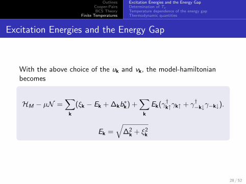
Excitation Energies and the Energy Gap

With the above choice of the uk and vk, the model-hamiltonianbecomes

HM − µN =∑k

(ξk − Ek + ∆kb∗k) +

∑k

Ek(γ†k↑γk↑ + γ†−k↓γ−k↓).

Ek =√

∆2k + ξ2k

28 / 52


Finite Temperatures



0

0.5

1

1.5

2

2.5

3

3.5

4

-3 -2 -1 0 1 2 3

Ek/

∆

ξk/∆

EksEkn

Figure: Energies of elementary excitations in the normal andsuperconducting states as functions of ξk.

29 / 52


Finite Temperatures



Inserting the γ operators in the definition of ∆k gives

∆k = −∑

l

Vkl 〈c−l↓cl↑〉

= −∑

l

Vklu∗l vl

⟨1− γ†l↑γl↑ − γ†−l↓γ−l↓

⟩= −

∑l

Vklu∗l vl(1− 2f (El))

= −∑

l

Vkl∆l

2Eltanh

βEl

2

30 / 52


Finite Temperatures



Using again the approximated potential Vkl = −V , we have∆k = ∆l = ∆ and therefor

1

V=

1

2

∑k

tanh(βEk/2)

Ek.

This formula determines the critical temperature Tc !

31 / 52


Finite Temperatures


Determination of Tc

The critical temperature Tc is the temperature at which ∆k → 0and thus Ek → ξk. By inserting this in the above formula,rewriting the sum as an integral and changing to a dimensionlessvariable we find

1

N(0)V=

∫ βc~ωc/2

0

tanh x

xdx = ln

(2eγ

πβc~ωc

)(γ ≈ 0.577...: the Euler constant)

32 / 52


Finite Temperatures


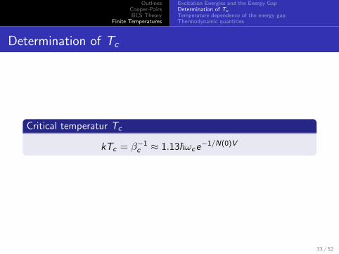
Determination of Tc

Critical temperatur Tc

kTc = β−1c ≈ 1.13~ωce

−1/N(0)V

33 / 52


Finite Temperatures


Determination of Tc

For small temperatures we find

1

N(0)V=

∫ ~ωc

0

dξ

(ξ2 + ∆2)1/2

⇒ ∆ =~ωc

sinh(1/N(0)V )≈ 2~ωce

−1/N(0)V ,

which shows that Tc and ∆(0) are not independent from eachother

∆(0)

kTc≈ 2

1.13≈ 1.764

34 / 52


Finite Temperatures


Temperature dependence of the energy gap

Rewriting again1

V=

1

2

∑k

tanh(βEk/2)

Ek.

in an integral form and inserting Ek gives

1

N(0)V=

∫ ~ωc

0

tanh 12β(ξ2 + ∆2)1/2

(ξ2 + ∆2)1/2dξ,

which can be evaluated numerically.

35 / 52


Finite Temperatures



Figure: Temperature dependence of the energy gap with someexperimental data (Phys. Rev. 122, 1101 (1961))

36 / 52


Finite Temperatures



Near Tc we get

Temperature dependence of ∆

∆(T )

∆(0)≈ 1.74

(1− T

Tc

)1/2

, T ≈ Tc ,

which shows the typical square root dependence of the orderparameter for a mean-field theory.

37 / 52


Finite Temperatures


Thermodynamic quantities

With ∆(T ) determined, we know the fermion excitation energies

Ek =√ξ2k + ∆(T )2. Then the quasi-particle occupation numbers

will follow the Fermi-function fk = (1 + eβEk)−1, which determinethe

electronic entropy for a fermion gas

Ses = −2k∑k

((1− fk) ln(1− fk) + fk ln fk).

38 / 52


Finite Temperatures



Figure: Electronic entropy in the superconducting and normal state.

39 / 52


Finite Temperatures



Given Ses(T ), we find the

specific heat

Ces = −β dSes

dβ= 2βk

∑k

− ∂fk∂Ek

(E 2

k +1

2β

d∆2

dβ

)In the normal state we have

Cen =2π2

3N(0)k2T .

40 / 52


Finite Temperatures



We expect a jump in the specific heat from the superconducting tothe normal state:

∆C = (Ces − Cen)|Tc= N(0)

(−d∆2

dT

)∣∣∣∣Tc

≈ 9.4N(0)k2Tc

41 / 52


Finite Temperatures



Figure: Experimental data for the specific heat in the superconductingand normal state (Phys. Rev. 114, 676 (1959))

42 / 52


Finite Temperatures


Type I superconductors

0

0.2

0.4

0.6

0.8

1

0 0.2 0.4 0.6 0.8 1

H

T/Tc

M-O-State

Normal-State

Figure: Phase diagram of a Type I superconductor

43 / 52


Finite Temperatures


Vortex-State

Original publication: Zh. Eksperim. i Teor. Fiz. 32, 1442 (1957)(Sov. Phys. - JETP 5, 1174 (1957))

44 / 52


Finite Temperatures


Type I and Type II superconductors

By applying Ginzburg-Landau theory for superconductors one findstwo characteristic lengths:

1 The Landau penetration depth for external magnetic fields λand

2 the Ginzburg-Landau coherence length ξ, which characterizesthe distance over which ψ can vary without undue energyincrease.

45 / 52


Finite Temperatures


Type I and Type II superconductors

Define

Ginzburg-Landau parameter

κ ≡ λ

ξ

By linearizing the GL equations near Tc one can find:

κ < 1√2: Type I superconductor

κ > 1√2: Type II superconductor

46 / 52


Finite Temperatures


Type II superconductors

0

0.5

1

1.5

2

2.5

3

0 0.2 0.4 0.6 0.8 1

H

T/Tc

M-O-State

Vortex-State

Normal-State

Figure: Phase diagram of a Type II superconductor

47 / 52


Finite Temperatures


As a solution of the GL equation, one could find the following formof the orderparameter:

Ψ(x , y) =1

N

∞∑n=−∞

exp

(π(ixy − y2)

ω1=ω2+ iπn

+iπ(2n + 1)

ω1(x + iy) + iπ

ω2

ω1n(n + 1)

)

N =

(ω1

2=ω2exp

(π=ω2

ω1

))1/4

48 / 52


Finite Temperatures


Vortex-State

-2 -1 0 1 2-2

-1

0

1

2

-2 -1 0 1 2-2

-1

0

1

2

Figure: Square and triangle symmetric state of the vortex lattice in adensity plot of |Ψ|2.

49 / 52


Finite Temperatures


Vortex-State

-2-1

01

2x

-2

-1

0

1

2

y

0

0.5

1ÈYÈ2

-2-1

01

2x

-2-1

01

2x

-2

-1

0

1

2

y

0

0.5

1ÈYÈ2

-2-1

01

2x

Figure: Square and triangle symmetric state of the vortex lattice in a 3Dplot.

50 / 52


Finite Temperatures


Summary

An attractive interaction between electrons will result informing bound Cooper pairs.

The model-hamiltonian can be diagonalized using aBogoliubov-Valatin-Transformation.

The order parameter in a superconductor is the energy-gap ∆.

BCS-Theory gives a prediction of the critical temperature Tc

and the energy gap ∆(T ).

Vortices will be observed in Type II superconductors.

51 / 52


Finite Temperatures


The END

Thank you for your attention!

Are there any questions?

52 / 52

bcs theory of superconductivity - katzgraber

Documents