bayesian regularisation priors

Bayesian Regularisation Priors

Thomas Kneib

Department of StatisticsLudwig-Maximilians-University Munich

21.1.2008

Thomas Kneib Outline

Outline

• Regularising Geoadditive Regression Models(with Ludwig Fahrmeir)

• Regularisation Priors for High-Dimensional Predictors(with Ludwig Fahrmeir, Susanne Konrath & Fabian Scheipl)

Bayesian Regularisation Priors 1

Thomas Kneib Leukemia Survival Data

Leukemia Survival Data

• Survival time of adults after diagnosis of acute myeloid leukemia.

• 1,043 cases diagnosed between 1982 and 1998 in Northwest England.

• 16 % (right) censored.

• Continuous and categorical covariates:

age age at diagnosis,wbc white blood cell count at diagnosis,sex sex of the patient,tpi Townsend deprivation index.

• Spatial information in different resolution.


Thomas Kneib Leukemia Survival Data

• Classical Cox proportional hazards model:

λ(t; x) = λ0(t) exp(x′γ).

• Baseline-hazard λ0(t) is a nuisance parameter and remains unspecified.

• Estimate γ based on the partial likelihood.

• Questions / Limitations:

– Estimate the baseline simultaneously with covariate effects.

– Flexible modelling of covariate effects (e.g. nonlinear effects, interactions).

– Spatially correlated survival times.

– Non-proportional hazards models / time-varying effects.

⇒ Geoadditive hazard regression models.


Thomas Kneib Geoadditive hazard regression

Geoadditive hazard regression

• Replace usual parametric predictor with a flexible semiparametric predictor

λ(t; ·) = λ0(t) exp[f1(age) + f2(wbc) + f3(tpi) + fspat(si) + γ1sex]

and absorb the baseline

λ(t; ·) = exp[f0(t) + f1(age) + f2(wbc) + f3(tpi) + fspat(si) + γ1sex]

where

– f0(t) = log(λ0(t)) is the log-baseline-hazard,

– f1, f2, f3 are nonparametric functions of age, white blood cell count anddeprivation, and

– fspat is a spatial function.

• Time-varying effects such as g1(t)sex can be included if needed.


Thomas Kneib Penalised Splines

Penalised Splines

• Approximate a function f(x) or g(t) by a linear combination of B-spline basisfunctions

f(x) =∑

j

βjBj(x)



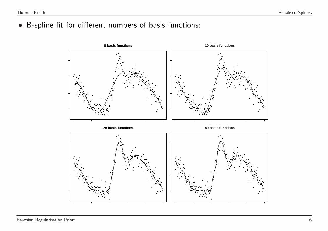
• B-spline fit for different numbers of basis functions:

5 basis functions 10 basis functions

20 basis functions 40 basis functions



• Unconstrained estimation crucially depends on the number of basis functions.

⇒ Add a regularisation term to the likelihood that enforces smoothness.

• Popular approach: Squared derivative penalty, e.g.

pen(f) = λ

∫(f ′′(x))2dx

• Easy approximation for B-splines: Difference penalties, e.g.

pen(β) = λ∑

j

(βj − βj−1)2 = λβ′Kβ

• Smoothing parameter λ governs the impact of the penalty (should be estimated).

• Corresponds to random walk prior in a Bayesian setting

βj = βj−1 + uj, uj ∼ N(0, τ2).



• Joint prior distribution is multivariate Gaussian

p(β) ∝ exp(− 1

2τ2β′Kβ

).

• The penalty corresponds to the log-prior.


Thomas Kneib Spatial Effects

Spatial Effects

• Regional data: Estimate a separate parameter βs for each region.

• Estimation becomes unstable if the number of regions is large relative to the samplesize.

⇒ Regularised estimation to enforce spatial smoothness.

• Effects of neighboring regions (common boundary) should be similar.

• Define a penalty term based on differences between neighboring parameters:

pen(β) = λ∑

s

∑

r∈N(s)

(βs − βr)2

where N(s) denotes the set of neighbors of region s.



• In a stochastic formulation equivalent to a Markov random field prior

βs =1

|N(s)|∑

r∈N(s)

βr + us, us ∼ N

(0,

τ2

|N(s)|)

• Again the joint prior distribution is multivariate Gaussian

p(β) ∝ exp(− 1

2τ2β′Kβ

)

where K is an adjacency matrix and

pen(β) = − log(p(β)).



• Individual data: Estimate a separate parameter βs for each distinct locations = (sx, sy).

• Smoothness assumption: The correlation of the spatial effect between two points s1

s2 can be described in terms of a parametric correlation function, e.g.

ρ(s1, s2) = ρ(||s1 − s2||) = exp(−α||s1 − s2||).

• More precisely: {βs, s ∈ R2} is assumed to follow a zero-mean stationary Gaussianrandom field.

• Well-known as Kriging in geostatistics.

• Results in a multivariate Gaussian prior for the spatial effects.


Thomas Kneib Bayesian Inference

Bayesian Inference

• Unifying framework:

– All vectors of function evaluations can be written as the product of a design matrixXj and a vector of regression coefficients βj, i.e. fj = Xjβj.

– Regularisation penalties are quadratic forms λjβ′jKjβj corresponding to Gaussian

priors

p(β|τ2) ∝ exp

(− 1

2τ2j

β′jKjβj

).

– The variance τ2j is a transformation of the smoothing parameter λj.

• The unifying framework allows to devise equally general inferential procedures.

• Implemented in the stand-alone software BayesX.


Thomas Kneib Bayesian Inference

• Mixed model based empirical Bayes inference:

– Consider the variances / smoothing parameters as unknown constants to beestimated by mixed model methodology.

– Decompose the vector of regression coefficients into (unpenalised) fixed effectsand (penalised) random effects.

– Penalised likelihood estimation of the regression coefficients in the mixed model(posterior modes).

– Marginal likelihood estimation of the variance and smoothing parameters (Laplaceapproximation).

• Fully Bayesian inference based on Markov Chain Monte Carlo simulation techniques:

– Assign inverse gamma priors to the variance / smoothing parameters.

– Metropolis-Hastings update for the regression coefficients (based on IWLS-proposals).

– Gibbs sampler for the variances (inverse gamma with updated parameters).


Thomas Kneib Results

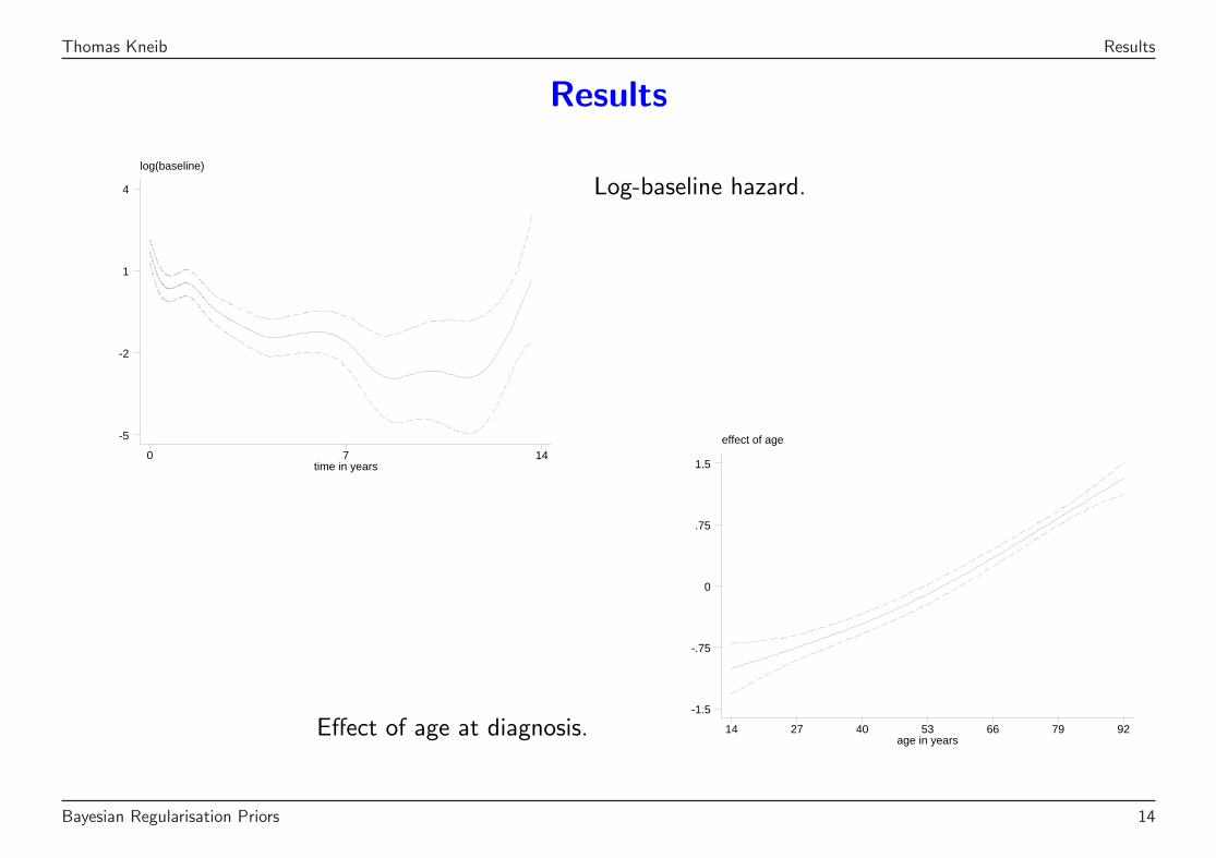
Results

log(baseline)

time in years0 7 14

-5

-2

1

4 Log-baseline hazard.

Effect of age at diagnosis.

effect of age

age in years14 27 40 53 66 79 92

-1.5

-.75

0

.75

1.5



effect of white blood cell count

white blood cell count0 125 250 375 500

-.5

0

.5

1

1.5

2 Effect of white blood cell count.

Effect of deprivation.

effect of townsend deprivation index

townsend deprivation index-6 -2 2 6 10

-.5

-.25

0

.25

.5



-0.44 0 0.3

District-level analysis−0.44 0.3

Individual-level analysis


Thomas Kneib Summary I

Summary I

• Geoadditive hazard regression provides a flexible model class for analysing survivaltimes.

• The software also supports more general censoring schemes, including left and intervalcensoring.

• Boosting-based methods for model choice and variable selection are currently underdevelopment.

• Similar models are available in the context of generalised linear models and categoricalregression.


Thomas Kneib Penalisation Approaches for High-Dimensional Predictors

Penalisation Approaches for High-Dimensional Predictors

• Regularisation in regression models with a large number of covariates: Enforce sparsemodels where most of the regression coefficients are (close to) zero.

• Examples include gene expression data but also social science and economicapplications.

• Most well-known approach: Ridge regression in the Gaussian model

y = Xβ + ε

• Estimation of β becomes numerically unstable for a large number of covariates

⇒ Add a quadratic penalty to the least squares criterion:

LSpen(β) = (y −Xβ)′(y −Xβ) + λ

p∑

j=1

β2j → min

β.



• Closed form solution: Penalised least squares (PLS) estimate

β̂ = (X ′X + λI)−1X ′y

• The PLS estimate is biased, but has a reduced variance compared to the least squaresestimate.

• Suitable choices of the smoothing parameter (for example by cross validation) shouldyield a reduced mean squared error.

• Essential for deriving the PLS estimate: The penalty term is differentiable withrespect to β.

• Drawback: Ridge regression typically does not induce enough sparsity.

⇒ Consider penalties that have a spike in zero.



• LASSO: Replace quadratic penalty with absolute value penalty:

LSpen(β) = (y −Xβ)′(y −Xβ) + λ

p∑

j=1

|βj| → minβ

.

ridge

−1.5 −1.0 −0.5 0.0 0.5 1.0 1.5

0.0

0.5

1.0

1.5

2.0

lasso

−1.5 −1.0 −0.5 0.0 0.5 1.0 1.5

0.0

0.5

1.0

1.5

2.0

• No closed form solution available, but efficient algorithms exist for purely linearmodels.



• LASSO imposes more sparseness and is able to set coefficients equal to zero.

• Other types of regularisation penalties:

– Lp-penalties:

pen(β) = λ

p∑

j=1

|βj|p, 0 ≤ p ≤ 2.

– Bridge-penalty:

pen(β) = λ1

p∑

j=1

|βj|+ λ2

p∑

j=1

β2j .

• Algorithms exist for linear models but become increasingly complex when consideringnon-Gaussian responses or combinations with geoadditive regression terms.

⇒ Can we benefit from a Bayesian formulation?


Thomas Kneib Regularisation Priors

Regularisation Priors

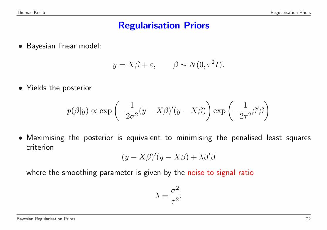
• Bayesian linear model:

y = Xβ + ε, β ∼ N(0, τ2I).

• Yields the posterior

p(β|y) ∝ exp(− 1

2σ2(y −Xβ)′(y −Xβ)

)exp

(− 1

2τ2β′β

)

• Maximising the posterior is equivalent to minimising the penalised least squarescriterion

(y −Xβ)′(y −Xβ) + λβ′β

where the smoothing parameter is given by the noise to signal ratio

λ =σ2

τ2.



• Posterior mode for Gaussian prior is equivalent to the PLS (ridge) estimate.

• The analogy carries over to more general types of priors:

Penalty Prior density Distribution

Ridge p(βj) ∝ exp(−λβ2j ) Gauss

LASSO p(βj) ∝ exp(−λ|βj|) Laplace

Lp p(βj) ∝ exp(−λ|βj|p) Powered exponential

Bridge p(βj) ∝ exp(−λ1|βj|) + exp(−λ2β2j ) Mixture

• Instead of maximising the posterior, consider simulation based estimation of theposterior mean.



• Advantages of MCMC simulation:

– Modular framework allows for immediate combination with nonparametric or spatialeffects.

– Hyperpriors for further model parameters yield a fully automated estimationscheme.

– Credible intervals for all parameters are available.

• Difficulty: Constructing appropriate proposal densities.

– The Gaussian prior is conjugate for Gaussian responses and yields a Gibbs samplingscheme.

– For non-Gaussian responses and Gaussian priors, adaptive proposal densities havebeen constructed based on iteratively weighted least squares proposals.

– For non-Gaussian priors, new proposal densities have to be developed, e.g. randomwalk proposals.

– Difficult due to the spike at zero.


Thomas Kneib Scale Mixtures of Normals

Scale Mixtures of Normals

• Popular idea in robust Bayesian approaches if the Gaussian distribution seems to bequestionable: Specify a hierarchical model, where

y|σ2 ∼ N(µ, σ2), σ2 ∼ IG(a, b).

• Marginally, y follows a t-distribution but sampling can be based on Gaussian responseswith inverse gamma hyperprior on the variance.

• Similarly, several regularisation priors can be written as scale mixtures of normals, i.e.

p(βj|λ) =∫ ∞

0

p(βj|τ2j )p(τ2

j |λ)dτ2j

whereβj|τ2

j ∼ N(0, τ2j ) and τ2

j |λ ∼ p(τ2j |λ).



• For the LASSO:

τ2j |λ ∼ Exp

(λ2

2

).

• Bayesian interpretation: Hierarchical prior formulation.

&%'$

&%'$

&%'$

&%'$

&%'$

- - -λ β λ τ2 βvs.

Lap(λ) Exp(0.5λ2) N(0, τ2)

• Advantage: Estimation based on MCMC recurs to the computationally simpler caseof ridge regression with an additional update step for the variances.

⇒ IWLS updates become available.

• Easily combined with nonparametric or spatial effects.

• Also applicable for non-Gaussian regression models.



• The concept extends to other types of priors that can be written as scale mixture ofnormals.

• Example: Powered exponential prior

exp(−|βj|p) ∝∫ ∞

0

exp

(− β2

j

2τ2j

)1τ6j

sp/2

(1

2τ2j

)dτ2

j

where sp(·) is the density of the positive stable distribution with index p.


Thomas Kneib Example

Example

• Diabetes data also used in the LARS-paper by Efron et al. (2004).

• 442 observations on a measure of disease progression (response) shall be related tothe covariates

age age of the patientsex genderbmi body mass indexmap average blood preasuretc, ldl, hdl, tch, ltg, glu blood serum measurements

• Covariates are standardised and the response is centered.



• Compare six competing approaches:

– Ordinary least squares (LS),

– Bayes with noninformative prior (B),

– Ridge regression (R),

– Bayesian ridge regression (BR),

– Frequentist LASSO (L),

– Bayesian LASSO (BL).

• Boxplots are based on 13-fold cross-validation (408 training cases and 34 test cases).


Thomas Kneib Summary II

Summary II

• Bayesian formulation allows to

– represent complex penalties in terms of Gaussian penalties via scale mixtures,

– re-use efficient algorithms derived for Gaussian priors,

– provides the full posterior, i.e. measures of uncertainty like credible intervals.

• Disadvantage: Small coefficients are no longer set to zero.

• Possible remedy: Mixed discrete-continuous distributions with a point mass in zero.

• Simpler approximation: Two-component continuous mixture, where one componentis concentrated around zero (despite being continuous).

• Find out more:

http://www.stat.uni-muenchen.de/~kneib


bayesian regularisation priors

Documents