This article was downloaded by: [UQ Library]On: 15 September 2013, At: 02:12Publisher: Taylor & FrancisInforma Ltd Registered in England and Wales Registered Number: 1072954 Registeredoffice: Mortimer House, 37-41 Mortimer Street, London W1T 3JH, UK

Statistics: A Journal of Theoretical andApplied StatisticsPublication details, including instructions for authors andsubscription information:http://www.tandfonline.com/loi/gsta20

Bayesian prediction of future numberof failures based on finite mixture ofgeneral class of distributionsYahia Abdel-Aty aa Department of Mathematics, Faculty of Science, Al-AzharUniversity, Nasr City, 11884, Cairo, EgyptPublished online: 09 Nov 2010.

To cite this article: Yahia Abdel-Aty (2012) Bayesian prediction of future number of failures basedon finite mixture of general class of distributions, Statistics: A Journal of Theoretical and AppliedStatistics, 46:1, 111-122, DOI: 10.1080/02331888.2010.500736

To link to this article: http://dx.doi.org/10.1080/02331888.2010.500736

PLEASE SCROLL DOWN FOR ARTICLE

Taylor & Francis makes every effort to ensure the accuracy of all the information (the“Content”) contained in the publications on our platform. However, Taylor & Francis,our agents, and our licensors make no representations or warranties whatsoever as tothe accuracy, completeness, or suitability for any purpose of the Content. Any opinionsand views expressed in this publication are the opinions and views of the authors,and are not the views of or endorsed by Taylor & Francis. The accuracy of the Contentshould not be relied upon and should be independently verified with primary sourcesof information. Taylor and Francis shall not be liable for any losses, actions, claims,proceedings, demands, costs, expenses, damages, and other liabilities whatsoever orhowsoever caused arising directly or indirectly in connection with, in relation to or arisingout of the use of the Content.

This article may be used for research, teaching, and private study purposes. Anysubstantial or systematic reproduction, redistribution, reselling, loan, sub-licensing,systematic supply, or distribution in any form to anyone is expressly forbidden. Terms &Conditions of access and use can be found at http://www.tandfonline.com/page/terms-and-conditions

Statistics, Vol. 46, No. 1, February 2012, 111–122

Bayesian prediction of future number of failures basedon finite mixture of general class of distributions

Yahia Abdel-Aty*

Department of Mathematics, Faculty of Science, Al-Azhar University, Nasr City 11884, Cairo, Egypt

(Received 25 September 2009; final version received 8 June 2010 )

This paper is concerned with the Bayesian prediction problem of the number of components which willfail in a future time interval. The failure times are distributed according to a finite mixture of a generalclass of distributions. Type-I censored sample from this nonhomogeneous population and a general classof prior density functions are used. A one-sample scheme is used to predict the number of failures in afuture time interval. An example of a finite mixture of k exponential components is given to illustrate ourresults.

Keywords: lifetime distribution; Bayesian prediction; mixture; type-I censoring

1. Introduction

In life testing, reliability and quality control problems, mixed failure populations are sometimesencountered. Mixture distributions comprise a finite or infinite number of components, possiblyof different distributional types, that can describe different features of data.

In life testing, the failure time population is not homogenous but can be a mixture of distinctlifetime distributions mixed in unknown proportions. Each of these distributions can represent adifferent type of failure for the population.

Studies including dedicated monographs, survey and review papers about finite mixture distri-butions were presented by several authors. Among others, are Everitt and Hand [1], Gupta [2],Titterington et al. [3], McLachlan and Basford [4] and Lindsay [5].

Bayesian prediction under a mixture of two exponential components model based on type-Icensoring has been studied by AL-Hussaini [6]. The same Bayesian prediction study based onfinite mixtures of Lomax components model has been studied by AL-Hussaini et al. [7].

Studying prediction of future number of failures is important because this problem is found inareas such as safety analysis of nuclear reactors and of aerospace systems. This study has beenpresented by Calabria and Pulcini [8] using Weibull distribution, and by Rashwan [9] using amixture of two exponential distributions.

*Email: yahia1970@yahoo.com

ISSN 0233-1888 print/ISSN 1029-4910 online© 2012 Taylor & Francishttp://dx.doi.org/10.1080/02331888.2010.500736http://www.tandfonline.com

Dow

nloa

ded

by [

UQ

Lib

rary

] at

02:

12 1

5 Se

ptem

ber

2013

112 Y. Abdel-Aty

For details on prediction, see Aitcheson and Dunsmore [10] and Geisser [11]. Distributionswith positive domain are particularly useful in life testing.

A general form of the class of distributions with positive domain includes, among others, theWeibull, three-parameter Burr-XII, Pareto type-I, beta, Gompertz and compound Gompertz dis-tributions. For more details about prediction studies of this class of distributions [12–14]. InSection 2, the probability function of the number of failures in a future time interval from themixed population is obtained. Each sub-population has a number of failure times in a speci-fied future time interval, the joint probability function of these numbers and the correspondingmarginal distributions are derived, where these marginal distributions are concerned with eachsub-population. The general prior and posterior density functions are derived too.

In Section 3, one sample prediction scheme based on type-I censored sample from the non-homogeneous population is used to obtain the predictive distribution of the number of failuresfrom the mixed population, the joint predictive distribution of the number of failures from eachsub-population and the corresponding marginal distributions are obtained. In Section 4, illustra-tive example of exponential distribution is given. Finally in Section 5, a numerical study using amixture of exponential distributions is given to illustrate the results.

2. Mixture distribution

A random variable X is said to follow a finite mixture distribution with k components if the densityfunction of X can be written in the following form,

f (x) =k∑

i=1

pifi(x), (1)

where pi is a non-negative real number (known as the ith mixing proportion) such that∑k

i=1 pi =1 and fi is the density function (known as the ith component), i = 1, . . . , k. The correspondingdistribution and reliability functions of X are given, respectively, by

F(x) =k∑

i=1

piFi(x), R(x) =k∑

i=1

piRi(x). (2)

Suppose that the failure time of the ith sub-population has the distribution function

Fi(x) ≡ F(x|θi) = 1 − exp[−λ(x|θi)] ≡ 1 − exp[−λi(x)] x > 0, (3)

where θi may be a vector and λi(x) ≡ λ(x; θi) is a non-negative continuous function of x suchthat λi(x) → 0 as x → 0+ and λi(x) → ∞ as x → ∞.

By writing f (x) ≡ f (x|θ), F (x) ≡ F(x|θ) and R(x) ≡ R(x|θ), where θ = (θ1, . . . , θk) ∈ �,it follows, from Equations (1) to (3), that the cumulative distribution function, the probabilitydensity function (pdf) and reliability function of the k-fold mixture are given, respectively, by

F(x) ≡ F(x|θ) = 1 −k∑

i=1

pi exp[−λi(x)] x > 0, (4)

f (x) ≡ f (x|θ) =k∑

i=1

piλ′i (x) exp[−λi(x)], x > 0, (5)

Dow

nloa

ded

by [

UQ

Lib

rary

] at

02:

12 1

5 Se

ptem

ber

2013

Statistics 113

and

R(x) ≡ R(x|θ) =k∑

i=1

pi exp[−λi(x)], x > 0, (6)

where λ′(x) = (d/dx)λ(x), R(x|θ) = 1 − F(x|θ).Suppose that n units from the population with density function (5) are subjected to the life

testing experiment and that the test is terminated after a predetermined time t (type-I censoring).Suppose that r units have failed during the test time, r1 units from the first sub-population, r2

units from the second sub-population, and so on till rk units from the kth sub-population. n − r

units are still functioning, where r = ∑ki=1 ri .

Suppose that xij ≤ t, i = 1, . . . , k, j = 1, . . . , ri , where xij denotes the failure time of thej th unit belonging to sub-population i.

Mendenhall and Hader [15] suggested such scheme of sampling to obtain the maximum-likelihood estimators of the parameters of mixed exponential distributions.

The following relation is obtained by using the binomial expansion and will be used throughoutthis paper, [

k∑i=1

bi

]n

=n∑

j1=0

j1∑j2=0

. . .

jk−2∑jk−1=0

cj1 . . . cjk−1bn−j11 . . . b

jk−2−jk−1k−1 b

jk−1k

=k∏

i=1

⎡⎣ ji−1∑ji=0

cjib

ji−1−ji

i

⎤⎦ , cji=

(ji−1

ji

), n ∈ N, (7)

where 0 = jk < · · · < ji < ji−1 < · · · < j0 = n and N is the set of natural numbers.In Equation (7) one may notice that, the dummy variable ji takes its values from 0 to ji−1 for

i = 1, . . . , k − 1, but the value of jk = 0 so jk is not a dummy variable of any sum, (i.e. for i = k

there is no sum but bjk−1k is a part of the last sum with dummy variable jk−1).

Using Equations (5)–(7) the likelihood function is given by

L(x|θ, p) ∝ [R(t)]n−r

k∏i=1

⎡⎣ ri∏j=1

pifi(xij )

⎤⎦∝

[k∑

i=1

pi exp[−λi(t)]]n−r k∏

i=1

⎡⎣pri

i Ai(xi.) exp

⎡⎣−ri∑

j=1

λi(xij )

⎤⎦⎤⎦∝

k∏i=1

⎡⎣ ji−1∑ji=0

cjip

ri+ji−1−ji

i Ai(xi.) exp

⎡⎣−ri∑

j=1

λi(xij ) − λi(t)(ji−1 − ji)

⎤⎦⎤⎦, (8)

where x = (x1., . . . , xk.), xi. = (xi1, . . . , xiri), θ = (θ1, . . . , θk), Ai(xi.) = ∏ri

j=1 λ′i (xij ), jk =

0, j0 = n − r, p = (p1, . . . , pk) and fi(xij ) denotes the density function of the failure times ofthe j th unit belonging to sub-population i.

Let M be a random variable representing the number of failures from the mixed population inthe future time interval (t, t∗]. By using Equations (6) and (7) the pdf of M [8] will be,

hM(m|θ, p) =(

n − r

m

)[R(t) − R(t∗)]m[R(t∗)]n−r−m[R(t)]−(n−r)

=(

n − r

m

)[R(t)]−(n−r)

m∑�=0

am� [R(t)]m−�[R(t∗)]n−r−m+�

Dow

nloa

ded

by [

UQ

Lib

rary

] at

02:

12 1

5 Se

ptem

ber

2013

114 Y. Abdel-Aty

=(

n − r

m

)[R(t)]−(n−r)

m∑�=0

am�

k∏i=1

⎡⎣ ji−1∑ji=0

li−1∑li=0

cjicli p

ji−1−ji+li−1−lii

× exp[−λi(t)(ji−1 − ji) − λi(t∗)(li−1 − li)]

⎤⎦, (9)

where am� = (−1)l

(m

�

), j0 = m − �, l0 = n − r − m + �, jk = lk = 0.

In the future time interval (t, t∗], we consider the number of failures M1 from the first sub-population, the number of failures M2 from the second sub-population, and so on till the number offailures Mk from the kth sub-population, being random variables denoted by, M = (M1, . . . , Mk),where M = ∑k

i=1 Mi and its value m satisfies that m ≤ n − r .By using Equations (6) and (7), the joint pdf of M1, M2, . . . , Mk [9] will be

gM(m|θ, p) = Cm[R(t)]−(n−r)[R(t∗)]n−r−m

k∏i=1

[pi[Ri(t) − Ri(t∗)]]mi

= Cm[R(t)]−(n−r)[R(t∗)]n−r−m

k∏i=1

⎡⎣pmi

i

mi∑�i=0

ami

�i[Ri(t)]mi−�i [Ri(t

∗)]�i

⎤⎦= Cm[R(t)]−(n−r)

k∏i=1

⎡⎣ mi∑�i=0

ji−1∑ji=0

ami

�icji

pji−1−ji+mi

i

× exp[−λi(t)(mi − �i) − λi(t∗)(ji−1 − ji + �i)]

⎤⎦, (10)

where Cm = (n − r)!/(m1! . . . mk!(n − r − m)!), m = (m1, . . . , mk), j0 = n − r − m, jk = 0.The marginal density function of the discrete random variable Ms is given by use of the joint

density (10) as follows:

�Ms(ms |θ, p) =

n1∑m1=0

. . .

ns−1∑ms−1=0

ns+1∑ms+1=0

. . .

nk∑mk=0

gM(m|θ, p)

=k∏

i=1i =s

ni∑mi=0

gM(m|θ, p), (11)

where s = 1, . . . , k, ni = n − r − ∑kj=1i =j

mj .

Suppose the general class of prior density functions of the parameters is given by

π(θ, p; δ) ∝ π1(θ; γ )π2(p; a)

∝k∏

i=1

pai−1i C(θi; γi) exp[−D(θi; γi)], (12)

where θi, pi are independent for i = 1, . . . , k and δ = (a, γ ) is the vector of hyper-parameters.It is also assumed that when θ1, . . . , θk are independent, then they may have the joint prior

Dow

nloa

ded

by [

UQ

Lib

rary

] at

02:

12 1

5 Se

ptem

ber

2013

Statistics 115

density function

π1(θ; γ ) ∝k∏

i=1

C(θi; γi) exp[−D(θi; γi)],

The parameters pi have a pdf of Dirichlet distribution of order k ≥ 2 with parametersa1, . . . , ak > 0 which is given by

π2(p; a) = 1

β(a)

k∏i=1

pai−1i ,

where β(a) is the multinomial beta function, which can be expressed in terms of the gammafunction:

β(a) =∏k

i=1 �(ai)

�(∑k

i=1 ai

) , a = (a1, . . . , ak).

Then from Equations (8) and (12) the joint posterior density function will be

π∗(θ, p; δ|x) = I−1n

k∏i=1

⎡⎣ ji−1∑ji=0

cjip

αi−1i η(θi; xi.) exp[−ζ(θi; xi.) − λi(t)(ji−1 − ji)]

⎤⎦, (13)

where αi = ri + ji−1 − ji + ai and In is the normalizing constant, which can be written as

In =k∏

i=1

⎡⎣∫θi

∫ 1

pi=0

ji−1∑ji=0

cjip

αi−1i η(θi; xi.) exp[−ζ(θi; xi.) − λi(t)(ji−1 − ji)] dpi dθi

⎤⎦=

k∏i=1

⎡⎣ ji−1∑ji=0

cjiβ(αi)

∫θi

η(θi; xi.) exp[−ζ(θi; xi.) − λi(t)(ji−1 − ji)] dθi

⎤⎦, (14)

whereη(θi; xi.) = Ai(xi.)C(θi; γi), ζ(θi; xi.) = ∑ri

j=1 λi(xij ) + D(θi; γi), and∏k

i=1 β(αi) is the

multinomial beta function, with β(αi) = �(αi)[�

(∑kν=1 αν

)]−1/k

.

3. One sample prediction scheme

In this section, we shall be concerned with the Bayesian prediction of the number of componentsfunctioning at time t , and that will fail in the future interval (t, t∗].

Using Equations (9) and (13), the Bayesian predictive density function of M given theobservations is given by

hM(m|x) =∫

θ

∫p

hM(m|θ, p)π∗(θ, p; δ|x) dp dθ

= Anm

m∑�=0

am�

k∏i=1

⎡⎣ ji−1∑ji=0

li−1∑li=0

cjicli

∫θi

∫ 1

pi=0p

ψi−1i η(θi; xi.)

× exp[−λi(t)(ji−1 − ji) − λi(t∗)(li−1 − li) − ζ(θi; xi.)] dpi dθi

⎤⎦

Dow

nloa

ded

by [

UQ

Lib

rary

] at

02:

12 1

5 Se

ptem

ber

2013

116 Y. Abdel-Aty

= Anm

m∑�=0

am�

k∏i=1

⎡⎣ ji−1∑ji=0

li−1∑li=0

cjicli β(ψi)

∫θi

η(θi; xi.)

× exp[−λi(t)(ji−1 − ji) − λi(t∗)(li−1 − li) − ζ(θi; xi.)] dθi

⎤⎦, (15)

where ψi = ji−1 − ji + li−1 − li + ri + ai, Anm = I−1n

(n−r

m

).

The joint predictive density function of M1, M2, . . . , Mk can be obtained by using Equa-tions (10) and (13) as follows:

gM(m|x) =∫

θ

∫p

gM(m|θ, p)π∗(θ, p; δ|x) dp dθ

= Cnm

k∏i=1

⎡⎣ mi∑�i=0

ji−1∑ji=0

ami

�icji

∫θi

∫ 1

pi=0p

φi−1i η(θi; xi.)

× exp[−λi(t)(mi − �i) − λi(t∗)(ji−1 − ji + �i) − ζ(θi; xi.)] dpi dθi

⎤⎦= Cnm

k∏i=1

⎡⎣ mi∑�i=0

ji−1∑ji=0

ami

�icji

β(φi)

∫θi

η(θi; xi.)

× exp[−λi(t)(mi − �i) − λi(t∗)(ji−1 − ji + �i) − ζ(θi; xi.)] dθi

⎤⎦, (16)

where φi = ji−1 − ji + mi + ri + ai, Cnm = I−1n Cm.

The marginal predictive distribution of Ms is given by

�Ms(ms |x) =

k∏i=1i =s

ni∑mi=0

gM(m|x)

=k∏

i=1i =s

ni∑mi=0

Cnm

k∏i=1

⎡⎣ mi∑�i=0

ji−1∑ji=0

ami

�icji

β(φi)

∫θi

η(θi; xi.)

× exp[−λi(t)(mi − �i) − λi(t∗)(ji−1 − ji + �i) − ζ(θi; xi.)] dθi

⎤⎦ (17)

Remark 1 If k = 2, then Equation (15) reduces to

hM(m|x) = A∗nm

m∑�=0

am�

⎡⎣m−�∑j=0

n∗+�∑l=0

cj cl

�(n − r2 − j − l + a1)�(r2 + a2 + j + l)

�(n + a1 + a2)

Dow

nloa

ded

by [

UQ

Lib

rary

] at

02:

12 1

5 Se

ptem

ber

2013

Statistics 117

×∫

θ1

∫θ2

η(θ1; x1.)η(θ2; x2.) exp[−λ2(t)j − λ2(t∗)l − ζ(θ2; x2.)]

× exp[−λ1(t)(m − j − �) − λ1(t∗)(n∗ − l + �) − ζ(θ1; x1.)] dθ1 dθ2

⎤⎦, (18)

where n∗ = n − r − m, am� = (−1)�

(m

�

), cj = (

m−�

j

), cl = (

n∗+�

l

), and

A∗nm =

(n − r

m

) ⎡⎣n−r∑j=0

(n − r

j

)β(n − r2 − j + a1, j + r2 + a2)

∫θ1

∫θ2

η(θ1; x1.)η(θ2; x2.)

× exp[−λ1(t)(n − r − j) − λ2(t)j − ζ(θ1; x1.) − ζ(θ2; x2.)] dθ1 dθ2

⎤⎦−1

.

Also, Equations (16) and (17) can be easily obtained when k = 2.

4. Mixture of exponential distributions

Let us now take an example of a failure population using a mixture of exponential distributions.In the case of exponential distributions, Equation (5) can be written in the following form:

f (x|θ) =k∑

i=1

piθi exp[−θix] x > 0, θi > 0, (19)

where λi(x) = θix.We study this population using different types of prior distributions as follows.

4.1. Gamma distribution

When the parameters pi, θi are unknown, we may use the gamma distribution as prior distributionfor θi , i.e. θi ∼ Gam(ci, di), where θ1, . . . , θk are independent and pi is independent of θi , thenthe class of prior distributions can be written as

π(θ, p; δ) ∝k∏

i=1

pai−1i θ

di−1i exp[−θici], ai > 0, ci > 0, di > 0. (20)

Therefore, C(θi; γi) = θdi−1i , D(θi; γi) = θici , and γi = (ci, di).

Also we have η(θi; xi.) = θdi+ri−1i , ζ(θi; xi.) = θi(ui + ci), where ui = ∑ri

j=1 xij .In can be obtained using Equation (14), so we have

In =k∏

i=1

⎡⎣ ji−1∑ji=0

cjiβ(αi)�(di + ri)[t (ji−1 − ji) + ui + ci]−(di+ri )

⎤⎦ . (21)

Our aim now is applying this mixture of exponential distributions to Equations (15)–(17).Then the Bayesian predictive density function of M , the joint predictive density function of

Dow

nloa

ded

by [

UQ

Lib

rary

] at

02:

12 1

5 Se

ptem

ber

2013

118 Y. Abdel-Aty

M1, M2, . . . , Mk and the marginal predictive density function of Ms are given, respectively, by

hM(m|x) = Anm

m∑�=0

am�

k∏i=1

⎡⎣ ji−1∑ji=0

li−1∑li=0

cjicli β(ψi)�(di + ri)

[t (ji−1 − ji) + t∗(li−1 − li) + ui + ci](di+ri )

⎤⎦, (22)

gM(m|x) = Cnm

k∏i=1

⎡⎣ mi∑�i=0

ji−1∑ji=0

ami

�icji

β(φi)�(di + ri)

[t (mi − �i) + t∗(ji−1 − ji + �i) + ui + ci](di+ri )

⎤⎦, (23)

�Ms(ms |x) =

k∏i=1i =s

ni∑mi=0

Cnm

k∏i=1

⎡⎣ mi∑�i=0

ji−1∑ji=0

ami

�icji

β(φi)�(di + ri)

[t (mi − �i) + t∗(ji−1 − ji + �i) + ui + ci](di+ri )

⎤⎦.

(24)

4.2. Inverse gamma distribution

The second case of the prior distribution for θi is the inverse gamma distribution, i.e. θi ∼IGam(ci, di), then the following is the joint prior density:

π(θ, p; δ) ∝k∏

i=1

pai−1i θ

−(di+1)i exp[−ci/θi], ai > 0, ci > 0, di > 0. (25)

It follows that

C(θi; γi) = θ−(di+1)i , D(θi; γi) = ci/θi, where γi = (ci, di),

η(θi; xi.) = θri−di−1i , and ζ(θi; xi.) = θiui + ci/θi . (26)

Substituting Equation (26) into Equation (14), then In is given by

In =k∏

i=1

⎡⎣ ji−1∑ji=0

2cjiβ(αi)Kri−di

(2√{t (ji−1 − ji) + ui}ci)

[{t (ji−1 − ji) + ui}/ci](ri−di )/2

⎤⎦. (27)

Again substituting Equation (26) into Equations (15)–(17), then the Bayesian predictive densityfunction of M , the joint predictive density function of M1, M2, . . . , Mk and the marginal predictivedensity function of Ms are given, respectively, by

hM(m|x) = Anm

m∑�=0

am�

k∏i=1

⎡⎣ ji−1∑ji=0

li−1∑li=0

2cjicli β(ψi)

× Kri−di

(2√{t (ji−1 − ji) + t∗(li−1 − li) + ui}ci

)[{t (ji−1 − ji) + t∗(li−1 − li) + ui}/ci](ri−di )/2

], (28)

Dow

nloa

ded

by [

UQ

Lib

rary

] at

02:

12 1

5 Se

ptem

ber

2013

Statistics 119

gM(m|x) = Cnm

k∏i=1

⎡⎣ mi∑�i=0

ji−1∑ji=0

2ami

�icji

β(φi)

× Kri−di

(2√{t (mi − �i) + t∗(ji−1 − ji + �i) + ui}ci

)[{t (mi − �i) + t∗(ji−1 − ji + �i) + ui}/ci](ri−di )/2

], (29)

�Ms(ms |x) =

k∏i=1i =s

ni∑mi=0

Cnm

k∏i=1

⎡⎣ mi∑�i=0

ji−1∑ji=0

2ami

�icji

β(φi)

× Kri−di

(2√{t (mi − �i) + t∗(ji−1 − ji + �i) + ui}ci

)[{t (mi − �i) + t∗(ji−1 − ji + �i) + ui}/ci](ri−di )/2

]. (30)

Equations (27)–(30) are obtained by using the following integral:∫ ∞

0xa−1 exp[−bx − c/x] dx = 2(c/b)a/2Ka(2

√bc), (31)

where Ka(·) is a modified Bessel function of the second kind.

Remark 2 In the case of non-informative prior, assuming Jeffrey’s invariant prior for θi anda uniform prior for pi , the joint prior density is obtained by putting ai = 1, di = ci = 0 inEquations (20) or (25) as follows:

π(θ, p; γ ) ∝k∏

i=1

1

θi

, (32)

The Bayesian predictive density function of M , the joint predictive density function ofM1, M2, . . . , Mk and the marginal predictive density function of Ms can also be obtained byusing the values ai = 1, di = ci = 0 in Equations (22)–(24). Rashwan [9] studied this case whenk = 2.

5. Numerical results

In this section, we present an example of mixture of two exponential distributions (k = 2) toillustrate the predictive procedures discussed in Section 4. In this example, we use gammadistribution as a prior distribution of the parameters θi and beta distribution as a prior distri-bution of the parameters pi , for i = 1, 2. In Equation (20), we assumed the prior parameters(c1, d1) = (10, 5), (c2, d2) = (5, 4) and (a1, a2) = (5, 2). Let us call this joint prior, GAMD. Theprior information about the parameters of the distribution suggests that (θ1, θ2) = (0.5, 0.8) and(p1, p2) = (0.71, 0.29). Based on these values of the parameters, a sample of size n = 20 isgenerated from the mixture of two exponential components:

0.014491 0.394089 0.629445 0.732375 0.877478 0.928398 1.1057941.431761 1.660797 2.699530 2.990934 4.166855 4.388902 4.703974,

0.030009 0.106272 0.873930 1.341693 1.639607 3.499348

where the number of generated observations from the first sub-population is 14 and the numberof generated observations from second sub-population is 6. Suppose that the future time interval

Dow

nloa

ded

by [

UQ

Lib

rary

] at

02:

12 1

5 Se

ptem

ber

2013

120 Y. Abdel-Aty

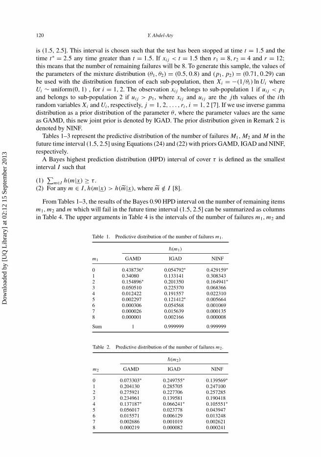
is (1.5, 2.5]. This interval is chosen such that the test has been stopped at time t = 1.5 and thetime t∗ = 2.5 any time greater than t = 1.5. If xij < t = 1.5 then r1 = 8, r2 = 4 and r = 12;this means that the number of remaining failures will be 8. To generate this sample, the values ofthe parameters of the mixture distribution (θ1, θ2) = (0.5, 0.8) and (p1, p2) = (0.71, 0.29) canbe used with the distribution function of each sub-population, then Xi = −(1/θi) ln Ui whereUi ∼ uniform(0, 1) , for i = 1, 2. The observation xij belongs to sub-population 1 if uij < p1

and belongs to sub-population 2 if uij > p1, where xij and uij are the j th values of the ithrandom variables Xi and Ui , respectively, j = 1, 2, . . . , ri , i = 1, 2 [7]. If we use inverse gammadistribution as a prior distribution of the parameter θ , where the parameter values are the sameas GAMD, this new joint prior is denoted by IGAD. The prior distribution given in Remark 2 isdenoted by NINF.

Tables 1–3 represent the predictive distribution of the number of failures M1, M2 and M in thefuture time interval (1.5, 2.5] using Equations (24) and (22) with priors GAMD, IGAD and NINF,respectively.

A Bayes highest prediction distribution (HPD) interval of cover τ is defined as the smallestinterval I such that

(1)∑

m∈I h(m|x) ≥ τ .(2) For any m ∈ I, h(m|x) > h(m|x), where m /∈ I [8].

From Tables 1–3, the results of the Bayes 0.90 HPD interval on the number of remaining itemsm1, m2 and m which will fail in the future time interval (1.5, 2.5] can be summarized as columnsin Table 4. The upper arguments in Table 4 is the intervals of the number of failures m1, m2 and

Table 1. Predictive distribution of the number of failures m1.

�(m1)

m1 GAMD IGAD NINF

0 0.438736∗ 0.054792∗ 0.429159∗1 0.34080 0.133141 0.3083432 0.154896∗ 0.201350 0.164941∗3 0.050510 0.225370 0.0683664 0.012422 0.191557 0.0223105 0.002297 0.121412∗ 0.0056646 0.000306 0.054568 0.0010697 0.000026 0.015639 0.0001358 0.000001 0.002166 0.000008

Sum 1 0.999999 0.999999

Table 2. Predictive distribution of the number of failures m2.

�(m2)

m2 GAMD IGAD NINF

0 0.073303∗ 0.249755∗ 0.139569∗1 0.204130 0.285705 0.2471002 0.275921 0.227706 0.2572853 0.234961 0.139581 0.1904184 0.137187∗ 0.066241∗ 0.105551∗5 0.056017 0.023778 0.0439476 0.015571 0.006129 0.0132487 0.002686 0.001019 0.0026218 0.000219 0.000082 0.000241

Dow

nloa

ded

by [

UQ

Lib

rary

] at

02:

12 1

5 Se

ptem

ber

2013

Statistics 121

Table 3. Predictive distribution of the number of failures m.

h(m)

m GAMD IGAD NINF

0 0.022184 0.001881 0.0388971 0.095771∗ 0.015619 0.127758∗2 0.197875 0.060950∗ 0.2163183 0.254710 0.145674 0.2429334 0.222792 0.232924 0.1958955 0.135282∗ 0.255003 0.1153166 0.055584 0.186705 0.048152∗7 0.014107 0.083655∗ 0.0129968 0.001691 0.017586 0.001732

Sum 1 1 1

Table 4. Bayes 0.90 HPD of the number of failures m1, m2 and m.

Bayes 0.90 HPD

Prior �(m1) �(m2) h(m)

GAMD [0, 2] [0, 4] [1, 5](0.934) (0.925) (0.906)

IGAD [0, 5] [0, 4] [2, 7](0.927) (0.902) (0.964)

NINF [0, 2] [0, 4] [1, 6](0.902) (0.939) (0.946)

m, respectively, where the bounds of each interval is the number of failures corresponding to thevalues remarked by asterisk inside the table of each case of the priors from Tables 1–3, and thelower arguments in Table 4 are the values of HPD (the sum of the values between the two asterisk).

6. Conclusion

In the above simulated sample, we notice that the remaining failures in the first sub-population are6 and the remaining failures in second sub-population are 2, and the number of failures m1, m2

and m in the future time interval (1.5, 2.5] is 1 , 1 and 2, respectively; the greatest value of HPDwith shortest length of the interval containing these values gives the best result. Therefore, theresult of GAMD prior is the best one.

Acknowledgements

The author appreciates the comments of the referees and the Editor which improved the first draft of this manuscript.

References

[1] B.S. Everitt and D.J. Hand, Finite Mixture Distributions, The University Press, Cambridge, UK, 1981.[2] S.S. Gupta, On mixtures of distributions: a survey and some new results on ranking and selection, Sankhya B 43

(1981), pp. 245–290.[3] D.M. Titterington, A.F. Smith, and V.E. Markov, Statistical Analysis of Finite Mixture Distributions, John Wiley and

Sons, New York, 1985.[4] G.J. McLachlan and K.E. Basford, Mixtures Models, Marcel Dekker, Inc., New York, 1988.

Dow

nloa

ded

by [

UQ

Lib

rary

] at

02:

12 1

5 Se

ptem

ber

2013

122 Y. Abdel-Aty

[5] B.G. Lindsay, Mixture Models: Theory, Geometry and Applications, NSF-CBMS Regional Conference Series inProbability and Statistics, Vol. 5, Institute of Mathematical Statistics, Beachwood, USA, 1995.

[6] E.K. AL-Hussaini, Bayesian prediction under a mixture of two exponential components model based on type Icensoring, J. Appl. Statist. Sci. 8 (1999), pp. 173–185.

[7] E.K. AL-Hussaini, A.M. Nigm, and Z.F. Jaheen, Bayesian prediction based on finite mixtures of Lomax componentsmodel and type I censoring, Statistics 35(3) (2001), pp. 259–268.

[8] R. Calabria and G. Pulcini, Bayes prediction of number of failures in Weibull samples, Comm. Statist. TheoryMethods 24(2) (1995), pp. 487–499.

[9] D.R. Rashwan, Bayes prediction for the number of failures in mixed exponential populations, Egyptian Statist. J.44(2) (2000), pp. 193–218.

[10] J. Aitcheson and I.R. Dunsmore, Statistical Prediction Analysis, Cambridge University Press, Cambridge, 1975.[11] S. Geisser, Predictive Inference: An Introduction, Chapman and Hall, London, 1993.[12] E.K. AL-Hussaini, Predicting observables from a general class of distributions, J. Statist. Plann. Inference 79(1)

(1999), pp. 79–91.[13] E.K. AL-Hussaini and A.A. Ahmed, On Bayesian predictive distributions of generalized order statistics, Metrika

57(2) (2003), pp. 165–176.[14] Y. Abdel-Aty, J. Franz, and M.A.W. Mahmoud, Bayesian prediction based on generalized order statistics using

multiply type-II censoring, Statistics 41(6) (2007), pp. 495–504.[15] W. Mendenhall and R.J. Hader, Estimation of parameters of mixed exponentially distributed failure time distributions

from censored life test data, Biometrika 45 (1958), pp. 504–520.

Dow

nloa

ded

by [

UQ

Lib

rary

] at

02:

12 1

5 Se

ptem

ber

2013