bayesian networks for the assessment of the effect of urbanization

Bayesian Networks for the Assessment of the Effect of Urbanization on Stream Macroinvertebrates

Kenneth H. Reckhow

Duke University [email protected]

Abstract

It is generally acknowledged that macroinvertebrates are good indicators of water quality in streams, as a number of taxa are sensitive to pollution and integrate their response to pollution over time. This fact has led some states (e.g., Maine) to incorporate macroinvertebrates in their water quality standards. To quantify the relationship between macroinvertebrates and urban land use, this study used data from the US Geological Survey “Effects of Urbanization on Stream Ecosystems” (EUSE) program. Bayesian networks were developed to characterize the relationship between urban land use metrics and selected macroinvertebrate taxa. It is shown that impervious surfaces and percent urban land have a strong effect on sensitive species of macroinvertebrates, demonstrating the adverse effect of urbanization and thus the value of these macroinvertebrate taxa as indicators of pollution. The resultant models are probabilistic and graphical, making them easily interpretable techniques for urban planning to achieve downstream water quality goals and sustain aquatic ecosystems.

Introduction

Ecologists [1, 2] have recognized that some

aquatic biota, such as macroinvertebrates, serve as integrators and indicators of water quality. This fact led the state of Maine to adopt a water quality standard based on macroinvertebrates and led other states (e.g., Ohio and North Carolina) to include stream macroinvertebrates in their ambient water quality monitoring programs. Since decisions on allowable pollutant loading to achieve compliance with water quality standards are typically guided with predictive models, there is a need for a predictive model relating land use to macroinvertebrate response. The objective of this paper is to develop a Bayesian network model of the impact of urbanization on macroinvertebrates

using the USGS EUSE (“Effects of Urbanization on Stream Ecosystems”) data. The paper begins with a brief description of the EUSE program and data; this is followed by a discussion of Bayesian networks and a presentation of the Bayes net structure learning approach employed here. Then, the urbanization-macroinvertebrate Bayes net models are developed and described. The paper concludes with a discussion of possible applications of the models. USGS EUSE Program

As part of the U.S. Geological Survey’s National

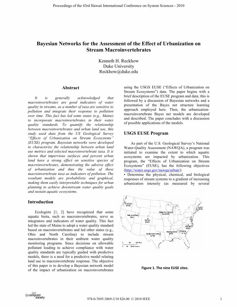
Water-Quality Assessment (NAWQA), a program was initiated to examine the extent to which aquatic ecosystems are impacted by urbanization. This program, the “Effects of Urbanization on Stream Ecosystems” (EUSE), has the following objectives (http://water.usgs.gov/nawqa/urban/): • Determine the physical, chemical, and biological responses of stream systems to a gradient of increasing urbanization intensity (as measured by several

Figure 1. The nine EUSE sites.

1

Proceedings of the 43rd Hawaii International Conference on System Sciences - 2010

978-0-7695-3869-3/10 $26.00 © 2010 IEEE

metrics). • Determine the most important landscape features driving hydrologic, chemical, geomorphic, habitat, and ecological responses to urbanization. • Determine the physical and chemical factors associated with biological responses. • Compare these responses among metropolitan areas located in different geographic settings (climate, geology, hydrology, biology, water use) across the United States.

Nine urban areas (see figure 1) were selected, and approximately 30 small watersheds were sampled in each of the nine urban areas. For each watershed, several urbanization characteristics (percent imperviousness, etc.) were measured. In the streams, physical characteristics (streamflow, water temperature, etc.), water chemistry (phosphorus, nitrogen, conductivity, etc.), and biological communities (algae, invertebrate, and fish metrics) were measured. Bayesian Networks

A Bayes network can be thought of as a

probabilistic graphical model with a series of nodes linked by arcs (arrows); see figure 2 below, or see [3] which presents a gentle introduction to Bayesian networks. In the Bayes network, the nodes represent important system variables, and the arcs indicate relationships between/among the variables. Each node is characterized by a marginal or conditional probability that expresses uncertain knowledge concerning that variable. The arcs between the nodes indicate conditional dependencies (i.e., each “down arc” variable is dependent on each “up arc” variable); variables that are not connected by arcs are

conditionally independent. The conditional dependencies may be quantified using any of the following: 1) mechanistic descriptions such as chemical reaction kinetics, 2) empirical relationships such as linear regression models, 3) relationships derived from elicited expert judgment, or 4) model structure learning algorithms. Application of a learning algorithm is particularly appealing if one is uncertain as to the underlying relationships. The variety of options for development of a Bayes net makes the approach extremely flexible.

From a simulation, or predictive, modeling perspective, A Bayes net can be considered as an alternative to a statistical, or mechanistic, model. Thus, if the data or knowledge were sufficient, one could develop a statistical or mechanistic model; however, a Bayes net offers a flexible alternative when these other modeling approaches may not easily be undertaken. From a decision analytic perspective, a Bayes net is essentially an influence diagram without “management action” (or “decision”) and “utility” nodes (in other words, it is an influence diagram with only “chance” nodes). Influence diagrams are used in decision analysis to complement decision trees.

To fix ideas on the characteristics of a Bayes network, consider the simple example presented in [3] which is displayed in figure 2. This model describes the impact of nitrogen on algal blooms and anoxia (lack of dissolved oxygen) in the Neuse River Estuary in North Carolina. The model indicates that the node, or variable, “percent nitrogen load reduction” is conditionally dependent on the “percent forested buffer” surrounding streams flowing into the Neuse. Similarly, the node “nitrogen concentration” is conditionally dependent on the nodes “percent nitrogen load reduction” and “spring precipitation”,

Figure 2. A Bayes Network example

2


and so on. The nodes (spring precipitation, percent forested

buffer, and summer precipitation) with no entry arrows are called “parent nodes” and are characterized using marginal probability. The nodes with entry arrows are called “child nodes” and are characterized using conditional probabilities, since their values are conditional on their parent nodes.

The modeling process in a Bayes network begins with the development of the structure (nodes, dependencies, and independencies) as displayed in figure 2. Marginal and conditional probabilities for each node can then be determined based on expert elicitation, probability learning algorithms, or with Monte Carlo simulation using an existing model. The prior Bayes network (before revising or updating with new information) is then “solved”; solving the prior Bayes network allows the probabilities in the entire network to affect other probabilities according to a set of rules [4]. For example, prior to solving, the conditional probability for anoxia is dependent on only the variable “algal bloom”. By solving the entire network, probabilities for the other variables propagate through the network, resulting in a marginal probability for anoxia, based on the entire network structure and the probabilities for other variables. Bayes networks may be solved or updated using one of many Bayes net application programs, such as WinBUGS (mrc-bsu.cam.ac.uk/bugs/winbugs), Hugin (hugin.com) and Netica (norsys.com). Here, Hugin was used, leading to the prior probability model in figure 3.

Most of the Bayes net programs (e.g., Hugin and Netica) require discretization of the continuous

probability distributions, as displayed in figure 3. The green bars for each node box in figure 3 represent the prior probabilities associated with each of the discrete categories (or “bins”). For example, (in the absence of actual data), an expert estimated that there was a 60% chance that between 80 percent and 95 percent of the stream lengths in the watershed had a forested buffer; this is reflected in the length of the green bar and the number 60 for that discrete category in the “percent forested buffer” node.

Discretization permits rapid revision of the network probabilities based on new information, as revision or updating is based on simple formulas associated with the Dirichlet-multinomial conjugate probability distributions (see [5] for an explanation of conjugate distribution families). This approach was used in all of the modeling results in this paper that take account of new information.

Bayesian Network Structure Learning

As noted in the previous section, it is possible to

“learn” the structure of a Bayesian network from a set of data using one of several algorithms that have been developed relatively recently [6, 7]. Structure learning is particularly useful when the relationships among variables are uncertain. That is the case for the analysis of the impact of urbanization on macroinvertebrates, so structure learning was applied to specify the models presented in the next section.

In the Hugin Bayes net program, two structure learning algorithms are available: the PC (named after its authors, Peter and Clark) and NPC (Necessary Path

Figure 3. The Prior Bayes Net Model

3


Condition) algorithms. The PC algorithm has been previously applied [7] for structural equation model learning and has been subsequently used for learning in Bayesian networks.

For structural equation models, the essence of the PC algorithm is as follows. The algorithm begins with a fully connected network; in other words, all nodes (variables) are directly connected to all other nodes. Connections are sequentially evaluated using the statistical significance of partial correlation coefficients. Consider an example with nodes A, B, and C, where A and B are hypothesized to be “parents” (predictors) of C. If it is found that the partial correlation between A and C, given B, is not significantly different from zero, then the connection between A and C is removed. This process, involving the statistical significance of partial correlations, is continued for the entire network. This assessment of “conditional independence” is the basis for learning the structure (arcs, or dependencies) of a structural equation model.

For a Bayesian network involving discrete nodes, the χ2 test is used in the PC algorithm in place of the statistical significance of partial correlations; otherwise the algorithm is essentially the same. Using the example in the previous paragraph, based on the χ2 test, if the expected frequency in the cell (or bin) of the conditional probability Table (CPT) for node C conditional on nodes A and B is the same as the expected frequency for node C conditional on node B only, then we should remove the arc between A and C. In effect, these tests (partial correlation and χ2) indicate whether or not A provides useful information on C, given B.

The NPC algorithm in Hugin is particularly useful when structure learning is based on a limited dataset or a dataset with an uncertainty level that adversely affects structure determination. These conditions can lead to ambiguity as to whether an arc should be present or absent in a particular Bayes net and which direction the arc should point (e.g., either A to C, or C to A). To resolve these ambiguities, Hugin provides the user with a graphics screen displaying the ambiguous arcs, and the user can interact with this screen to resolve the ambiguous connections based on substantive knowledge.

The PC and NPC algorithms are effective strategies for discovering the underlying structure in multivariate data. Since both algorithms allow the user to input prior substantive knowledge about arcs (either their known presence or absence), the algorithms will generally yield a plausible model structure with a scientific expert and an informative dataset. However, neither algorithm is guaranteed to yield the best model based on two useful model selection criteria: the AIC

(Akaike Information Criterion) and the BIC (Bayesian Information Criterion). Both of these model selection criteria arise from information theory, and both (with slightly different formulations) reward parsimonious models with low model error. In other words, the AIC and BIC scores are best for models that explain more variance in the data with fewer variables (and fewer bins).

Thus, it seems plausible to consider more than one model that results from the Hugin structure learning algorithms and use AIC and BIC as another basis (besides compatibility with substantive knowledge, of course) for model selection. One additional statistic reported by Hugin that could be useful for final model selection is “mutual information.” The mutual information between two variables is:

∑∑∈ ∈

=Yy Xx ypxp

yxpyxpYXI ))()(

),(log(),();(21

(1)

Mutual information, reported in Hugin, represents

the information shared by X and Y; in other words, mutual information tells us how much does knowledge of X reduce our uncertainty concerning Y. Correspondingly, if X and Y are independent and thus knowing X tells us nothing about Y, then I(X;Y)=0.

Given the structure learning algorithms in Hugin, the AIC and BIC statistics, and the mutual information, the following model selected strategy was employed here. The NPC algorithm was initially applied, and ambiguous arcs were resolved with substantive knowledge. AIC and BIC were consulted, which tended to lead to more parsimonious models

Node Units Urban disturbance percent urban land cover in

basin area Hydrologic modifications

dams per 100 square kilometer basin area

Change in generation of flow

percent impervious surface

Hydrology stage rise ≥ five times the median stage rise (#times)

Habitat mean channel width to depth ratio

Water quality conductivity at low base flow (microsiemens per centimeter at 25OC)

EPT richness number of EPT taxa Richness-weighted tolerance

average tolerance of taxa at a site on a scale of 0-10

Percent intolerant taxa

percent of total richness composed of intolerant taxa

Table 1. Node definitions for the Bayes networks.

4


(fewer arcs). Finally, mutual information was examined and additional arcs were removed if it appeared that they contributed little to the goal of this model – linking urbanization metrics to macroinvertebrates. A Bayesian Network for the Impact of Urbanization on Macroinvertebrates

In the past year, we have applied Bayesian

networks and hierarchical models to the EUSE data to characterize multivariate relationships, initially focusing on the impact of urbanization on

macroinvertebrates. In this paper, the application of Bayes nets will be highlighted for 88 small watersheds

in the areas around Birmingham, AL., Atlanta, GA., and Raleigh, NC. Table 1 provides definitions for the variables in the EUSE Bayes net models.

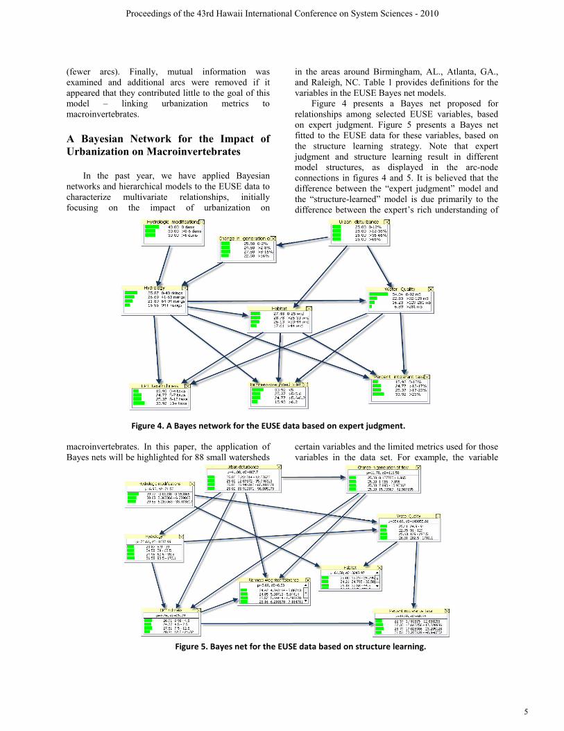
Figure 4 presents a Bayes net proposed for relationships among selected EUSE variables, based on expert judgment. Figure 5 presents a Bayes net fitted to the EUSE data for these variables, based on the structure learning strategy. Note that expert judgment and structure learning result in different model structures, as displayed in the arc-node connections in figures 4 and 5. It is believed that the difference between the “expert judgment” model and the “structure-learned” model is due primarily to the difference between the expert’s rich understanding of

certain variables and the limited metrics used for those variables in the data set. For example, the variable

Figure 5. Bayes net for the EUSE data based on structure learning.

Figure 4. A Bayes network for the EUSE data based on expert judgment.

5


“habitat” is a complex concept to aquatic ecologists; however in the EUSE data set, habitat is simply measured by the mean stream channel width to depth ratio at a site; this data set definition clearly does not fully describe the ecologists’ concept of habitat. Thus it is not surprising that the expert-based model might differ from the structure-learned model. If we were to combine an expert-learned prior Bayes net model with a structure-learned model, it is essential that variables in each model are defined/measured in the same metric.

It is instructive to describe the features of the Bayes networks in figures 4 and 5. In the figure 4 elicited model, the numeric percentage column on the left (equivalent to the length of the horizontal green bar) results from the initial expert elicitation of marginal and conditional probabilities and the structure of the elicited Bayes net model. In figure 5, the numeric column on the left indicates the percentage (equivalent to the length of the horizontal green bar) of the watershed sites that fall within the variable’s range as specified by the numeric column on the right. For example in figure 5, for the variable “water quality”, the left numeric column (and, graphically, the corresponding green bar) indicates that 23.0% of the watersheds in the dataset for this model application have conductivity between 24.9 and 91. Figure 5 is the baseline structurally-learned model that reflects data from the 88 small watersheds with bin sizes that result in approximately the same percentage of watersheds in each of the bins. Discrete bins could be established based on other criteria (e.g.,

equal ranges on each variable or expert judgment as in the Neuse Estuary example presented above). The equal percentage approach was chosen so that there would be a clear graphical impression (in subsequent Bayes nets presented below) of the effect of new (predictive) information for one variable on all other variables.

Figure 6 conveys a predictive application of the Bayes net model (the red bars represent a particular case for prediction). The model is predictive because it is predicting the impact of high percent urban land cover (node “urban disturbance”) and high percent impervious surface (node “change in generation of flow”) on the other nodes; this impact is expressed by the length of the green bars (and the percentages) for all other nodes. It is particularly noteworthy to observe the impact of these high urbanization conditions on the macroinvertebrate node “EPT richness.” EPT refers to macroinvertebrate taxa that are sensitive to polluted conditions. Thus one would expect that if urbanization and imperviousness contribute to water pollution, and these characteristics are high, then EPT taxa richness should be low; this is indeed the case in figure 6, when compared to figure 5 (the baseline case). Correspondingly, when the urbanization/impervious conditions are low, analysis indicates that EPT taxa richness is high.

Figure 7 presents a “back” prediction using a parsimonious model to assess what land use conditions are associated with the most desirable levels of the macroinvertebrate taxa. Note that, as expected, low macroinvertebrate impact is associated with low urban

Figure 6. A predictive Bayes net fitted to the EUSE data.

6


land use and high forested land use percentages in the watersheds.

The parsimonious model does not include the “intermediate” variables (e.g., water quality, habitat, and hydrology), as it seems likely that the metrics in the EUSE dataset for these variables contributed to their lack of importance (based on the mutual

information presented in figure 8). The problem with the habitat variable is discussed above; the problem with the water quality variable is that it reflects a one-time measurement, whereas macroinvertebrates integrate their response over time.

Figure 8. Mutual information for the EUSE model based on structure learning.

Figure 7. “Back predictions” of land cover associated with macroinvertebrate levels.

7


Conclusions

It is clear from the predictive applications of the Bayes net EUSE model in figure 6 that urban intensity, as measured by percent urban land cover and percent impervious surface, has an adverse effect on macroinvertebrate taxa. Thus, the results presented here are significant because they indicate that we can use the EUSE data to assess how selected urbanization metrics affect macroinvertebrates.

The back prediction Bayes net model (figure 7) is suggestive of a plausible strategy for future Bayes net model development. If the discrete categories for the ecosystem response variables include a breakpoint at the water quality standard, then a back prediction for the bin associated with standard compliance will yield conditions on manageable variables (e.g., percent urban land cover in a watershed) that are associated with compliance.

Further, the lack of importance of intermediate variables (e.g., habitat and water quality) that the expert believed were important has implications for future monitoring design and measurements. If monitoring is undertaken to provide data for a multivariate model, then variable definitions and metrics should be selected so that they express each variable in a manner that captures scientific understanding. So, for example, if it is believed that macroinvertebrates provide a time-integrated response to water quality, then the water quality measurements should not be single grab samples, instead they should be multiple samples collected over the relevant time period.

In conclusion, the Bayes net models that yielded these results easily can be applied by urban planners to guide urban redevelopment or new urban development so that effects on downstream aquatic ecosystems are managed and ecosystems are sustained. Further, the results are probabilistic, providing urban planners with an assessment of the chances of success of their proposed actions. Acknowledgments This research was supported by a cooperative agreement from the U.S. Geological Survey. Tom Cuffney, Roxolana Kashuba, and anonymous reviewers provided useful comments. References [1] Yoder, C.O. 1995. Policy Issues and Management Applications of Biological Criteria. In: Biological Assessment and Criteria: Tools for Water Resources

Planning and Decision Making, W.S. David and T.P. Simon (Editors). Lewis Publishers. Boca Raton, Florida. pp. 327-343. [2] Cuffney,T.F., Zappia, H., Giddings, E.M.P., and J.F. Coles. 2005. Effects of Urbanization on Benthic Macroinvertebrate Assemblages in Contrasting Environmental Settings: Boston, Massachusetts; Birmingham, Alabama; and Salt Lake City, Utah. American Fisheries Society Symposium. 47:361-407. [3] Reckhow, K.H. 1999. Water Quality Prediction and Probability Network Models. Canadian Journal of Fisheries and Aquatic Sciences.56:1150-1158. [4] Korb, K.B., and A.E. Nicholson. 2004. Bayesian Artificial Intelligence. Chapman & Hall. London. [5] Raiffa, H., and R.Schlaifer. 1961. Applied Statistical Decision Theory. MIT Press. Cambridge, MA. [6] Jensen, F. V., and T.D. Nielsen. 2007. Bayesian Networks and Decision Graphs. 2nd Ed. Springer. New York. [7] Spirtes, P., Glymour, C., and C. Meek. 1993. Causation, Prediction, and Search. Springer-Verlag. New York.

8


bayesian networks for the assessment of the effect of urbanization

Documents