University of Arkansas, FayettevilleScholarWorks@UARK

Theses and Dissertations

5-2018

Bayesian Network Modeling and Inference ofGWAS CatalogQiuping PanUniversity of Arkansas, Fayetteville

Follow this and additional works at: http://scholarworks.uark.edu/etd

Part of the Bioinformatics Commons, Genomics Commons, and the OS and NetworksCommons

This Thesis is brought to you for free and open access by ScholarWorks@UARK. It has been accepted for inclusion in Theses and Dissertations by anauthorized administrator of ScholarWorks@UARK. For more information, please contact scholar@uark.edu, ccmiddle@uark.edu.

Recommended CitationPan, Qiuping, "Bayesian Network Modeling and Inference of GWAS Catalog" (2018). Theses and Dissertations. 2709.http://scholarworks.uark.edu/etd/2709

Bayesian Network Modeling and Inference of GWAS Catalog

A thesis submitted in partial fulfillmentof the requirements for the degree of

Master of Science in Computer Science

by

Qiuping PanHuaqiao University

Bachelor of Network Engineering, 2009

May 2018University of Arkansas

This thesis is approved for recommendation to the Graduate Council.

Xintao Wu, Ph.D.Thesis Director

Wing Ning Li, Ph.D.Committee member

Qinghua Li, Ph.D.Committee member

Abstract

Genome-wide association studies (GWASs) have received an increasing attention to understand

genotype-phenotype relationships. The Bayesian network has been proposed as a powerful tool

for modeling single-nucleotide polymorphism (SNP)-trait associations due to its advantage in

addressing the high computational complex and high dimensional problems. Most current works

learn the interactions among genotypes and phenotypes from the raw genotype data. However,

due to the privacy issue, genotype information is sensitive and should be handled by complying

with specific restrictions. In this work, we aim to build Bayesian networks from publicly released

GWAS statistics to explicitly reveal the conditional dependency between SNPs and traits.

First, we focus on building a Bayesian network for modeling the SNP-categorical trait relation-

ships. We construct a three-layered Bayesian network explicitly revealing the conditional depen-

dency between SNPs and categorical traits from GWAS statistics. We then formulate inference

problems based on the dependency relationship captured in the Bayesian network. Empirical

evaluations show the effectiveness of our methods.

Second, we focus on modeling the SNP-quantitative trait relationships. Existing methods in the

literature can only deal with categorical traits. We address this limitation by leveraging the Con-

ditional Linear Gaussian (CLG) Bayesian network, which can handle a mixture of discrete and

continuous variables. A two-layered CLG Bayesian network is built where the SNPs are rep-

resented as discrete variables in one layer and quantitative traits are represented as continuous

variables in another layer. Efficient inference methods are then derived based on the constructed

network. The experimental results demonstrate the effectiveness of our methods.

Finally, we present STIP, a web-based SNP-trait inference platform capable of a variety of infer-

ence tasks, such as trait inference given SNP genotypes and genotype inference given traits. The

current version of STIP provides three services which are SNP-trait inference, Top-k trait predic-

tion and GWAS catalog exploration.

Acknowledgements

Foremost, I would like to express my sincere gratitude to my advisor Prof. Xintao Wu for the

continuous support of my master’s study and research, for his patience, motivation, and immense

knowledge. His guidance helped me in all time of research and writing of this thesis.

I would like to thank Dr. Lu Zhang, the postdoctoral fellow in our laboratory, for advising and

leading me working on the GWAS project, for his contributions to the theoretical results of this

work, and for the days we were working together for the deadlines. Part of this work is collabo-

rating with Dr. Xinhua Shi and Dr. Yue Wang, thank you for all the discussions and efforts.

My sincere thank also goes to my thesis committee members: Prof. Qinghua Li and Prof. WingN-

ing Li, for their insightful comments and suggestions. I would also like to thank everyone in the

Department of Computer Science and Computer Engineering and Graduate School at the Univer-

sity of Arkansas for their help and guidance.

To the rest of my lab members, Srinidhi Katla, Depeng Xu, Yongkai Wu, Panpan Zheng and

Yueyang Wang, thank you for all the fun we had in the last two years, and for your general help

and encouragement.

My completion of this thesis writing could not have been accomplished without the support of

my husband, Dr. Shuhan Yuan. Without his continuous help with reading and comments on this

thesis, I cannot successfully finish this work in a good shape. My heartfelt thanks.

Table of Contents

1 Introduction . . . . . . . . . . . . . . . . . . . . . . . . . . . . . . . . . . . . . . . . 1

1.1 Overview . . . . . . . . . . . . . . . . . . . . . . . . . . . . . . . . . . . . . . . 1

1.2 Contributions . . . . . . . . . . . . . . . . . . . . . . . . . . . . . . . . . . . . . 3

1.3 Organization of the Thesis . . . . . . . . . . . . . . . . . . . . . . . . . . . . . . 4

2 Background . . . . . . . . . . . . . . . . . . . . . . . . . . . . . . . . . . . . . . . . . 5

2.1 GWAS and GWAS Catalog . . . . . . . . . . . . . . . . . . . . . . . . . . . . . . 5

2.1.1 Genome-Wide Association Study (GWAS) . . . . . . . . . . . . . . . . . . 5

2.1.2 GWAS Catalog . . . . . . . . . . . . . . . . . . . . . . . . . . . . . . . . 8

2.2 Bayesian Network . . . . . . . . . . . . . . . . . . . . . . . . . . . . . . . . . . . 9

2.2.1 Independence of Causal Influence . . . . . . . . . . . . . . . . . . . . . . 10

2.2.2 CLG Bayesian Network . . . . . . . . . . . . . . . . . . . . . . . . . . . 13

3 Modeling SNP and Categorical Trait Association Using Bayesian Network . . . . . . 15

3.1 Introduction . . . . . . . . . . . . . . . . . . . . . . . . . . . . . . . . . . . . . . 15

3.2 Learning Bayesian Network from GWAS Statistics . . . . . . . . . . . . . . . . . 18

3.2.1 Knowledge from GWAS Catalog . . . . . . . . . . . . . . . . . . . . . . . 18

3.2.2 Three-layered Bayesian Network Construction . . . . . . . . . . . . . . . 19

3.2.3 Modeling SNP-Trait Associations . . . . . . . . . . . . . . . . . . . . . . 22

3.3 Inference Based on the Constructed Bayesian Network . . . . . . . . . . . . . . . 25

3.3.1 General Inference Formula . . . . . . . . . . . . . . . . . . . . . . . . . . 26

3.3.2 Trait Inference Given SNP Genotype . . . . . . . . . . . . . . . . . . . . . 28

3.3.3 Genotype Inference Given Trait . . . . . . . . . . . . . . . . . . . . . . . 30

3.3.4 Trait Inference Given Trait . . . . . . . . . . . . . . . . . . . . . . . . . . 31

3.3.5 Application: Identity Attack . . . . . . . . . . . . . . . . . . . . . . . . . 32

3.4 Further Extensions . . . . . . . . . . . . . . . . . . . . . . . . . . . . . . . . . . 32

3.5 Experiments . . . . . . . . . . . . . . . . . . . . . . . . . . . . . . . . . . . . . . 34

3.5.1 Noisy-Or Model Validation . . . . . . . . . . . . . . . . . . . . . . . . . . 34

3.5.2 Bayesian Network Construction . . . . . . . . . . . . . . . . . . . . . . . 37

3.5.3 Simulated Scenario: Trait Inference . . . . . . . . . . . . . . . . . . . . . 38

3.5.4 Simulated Scenario: Identity Inference . . . . . . . . . . . . . . . . . . . . 40

3.6 Related Work . . . . . . . . . . . . . . . . . . . . . . . . . . . . . . . . . . . . . 44

3.7 Summary . . . . . . . . . . . . . . . . . . . . . . . . . . . . . . . . . . . . . . . 47

4 Modeling SNP and Quantitative Trait Association Using CLG Bayesian Network . . 48

4.1 Introduction . . . . . . . . . . . . . . . . . . . . . . . . . . . . . . . . . . . . . . 48

4.2 Learning CLG Bayesian Network from GWAS Statistics . . . . . . . . . . . . . . 49

4.2.1 Knowledge from GWAS catalog . . . . . . . . . . . . . . . . . . . . . . . 49

4.2.2 CLG Bayesian Network Construction . . . . . . . . . . . . . . . . . . . . 51

4.3 Inference Based on the Constructed Bayesian Network . . . . . . . . . . . . . . . 56

4.4 Further Extensions . . . . . . . . . . . . . . . . . . . . . . . . . . . . . . . . . . 58

4.5 Experiments . . . . . . . . . . . . . . . . . . . . . . . . . . . . . . . . . . . . . . 59

4.5.1 CLG Bayesian Network Construction . . . . . . . . . . . . . . . . . . . . 60

4.5.2 Inference Evaluation . . . . . . . . . . . . . . . . . . . . . . . . . . . . . 61

4.5.3 Application: Identity Inference . . . . . . . . . . . . . . . . . . . . . . . . 62

4.6 Related Work . . . . . . . . . . . . . . . . . . . . . . . . . . . . . . . . . . . . . 64

4.7 Summary . . . . . . . . . . . . . . . . . . . . . . . . . . . . . . . . . . . . . . . 65

5 STIP: A SNP-Trait Inference Platform . . . . . . . . . . . . . . . . . . . . . . . . . . 66

5.1 Introduction . . . . . . . . . . . . . . . . . . . . . . . . . . . . . . . . . . . . . . 66

5.2 STIP Overview . . . . . . . . . . . . . . . . . . . . . . . . . . . . . . . . . . . . 67

5.2.1 Bayesian Network Construction . . . . . . . . . . . . . . . . . . . . . . . 67

5.2.2 Services Provided by STIP . . . . . . . . . . . . . . . . . . . . . . . . . . 71

5.3 Demonstration . . . . . . . . . . . . . . . . . . . . . . . . . . . . . . . . . . . . . 74

5.3.1 SNP-Trait Inference . . . . . . . . . . . . . . . . . . . . . . . . . . . . . . 74

5.3.2 Top-K Trait Prediction . . . . . . . . . . . . . . . . . . . . . . . . . . . . 75

5.3.3 GWAS Catalog Exploration . . . . . . . . . . . . . . . . . . . . . . . . . 76

5.4 Summary . . . . . . . . . . . . . . . . . . . . . . . . . . . . . . . . . . . . . . . 77

6 Conclusions and Future Work . . . . . . . . . . . . . . . . . . . . . . . . . . . . . . 78

6.1 Conclusions . . . . . . . . . . . . . . . . . . . . . . . . . . . . . . . . . . . . . . 78

6.2 Future Work . . . . . . . . . . . . . . . . . . . . . . . . . . . . . . . . . . . . . . 79

Bibliography . . . . . . . . . . . . . . . . . . . . . . . . . . . . . . . . . . . . . . . . . . 80

List of Figures

2.1 Examples of categorical traits in the GWAS catalog. . . . . . . . . . . . . . . . . . 8

2.2 Examples of quantitative traits in the GWAS catalog. . . . . . . . . . . . . . . . . 9

2.3 The ICI model . . . . . . . . . . . . . . . . . . . . . . . . . . . . . . . . . . . . . 11

3.1 A three-layered Bayesian network of traits and associated SNPs . . . . . . . . . . 20

3.2 Identity attack . . . . . . . . . . . . . . . . . . . . . . . . . . . . . . . . . . . . . 31

3.3 An example network where S 1 and S 2 are correlated. . . . . . . . . . . . . . . . . 32

3.4 Top-3 and bottom-3 traits of each CEU individual . . . . . . . . . . . . . . . . . . 39

3.5 (a) Average Probability of Identification; (b) Probability Distribution of Identifi-cation . . . . . . . . . . . . . . . . . . . . . . . . . . . . . . . . . . . . . . . . . 42

3.6 Probability of identification: (a) all targets; (b) targets with hypertriglyceridemia . . 44

4.1 The two-layered CLG Bayesian network . . . . . . . . . . . . . . . . . . . . . . . 51

4.2 Posteriori probability densities of traits. . . . . . . . . . . . . . . . . . . . . . . . 61

4.3 Posteriori probability distribution of SNPs. . . . . . . . . . . . . . . . . . . . . . . 62

4.4 Probability of identification. . . . . . . . . . . . . . . . . . . . . . . . . . . . . . 63

5.1 The architecture of STIP . . . . . . . . . . . . . . . . . . . . . . . . . . . . . . . 67

5.2 The information of SNP-trait associations stored in JSON files. . . . . . . . . . . 70

5.3 The procedures of SNP-trait inference and Top-k trait prediction . . . . . . . . . . 73

5.4 SNP-categorical trait inference web UI with an example of trait inference givenSNP genotypes and categorical traits . . . . . . . . . . . . . . . . . . . . . . . . . 74

5.5 Top-k trait prediction web UIs with results of trait prediction given a user’s ge-netic file . . . . . . . . . . . . . . . . . . . . . . . . . . . . . . . . . . . . . . . . 75

5.6 GWAS catalog exploration web UIs . . . . . . . . . . . . . . . . . . . . . . . . . 76

List of Tables

2.1 The genotype frequency . . . . . . . . . . . . . . . . . . . . . . . . . . . . . . . . 6

2.2 The allele frequency . . . . . . . . . . . . . . . . . . . . . . . . . . . . . . . . . . 6

3.1 SNP-Trait associations . . . . . . . . . . . . . . . . . . . . . . . . . . . . . . . . 36

3.2 The chi-square value, degree of freedom (df), p-value, RMSEA of the Noisy-ormodel . . . . . . . . . . . . . . . . . . . . . . . . . . . . . . . . . . . . . . . . . 36

3.3 Trait-SNP association . . . . . . . . . . . . . . . . . . . . . . . . . . . . . . . . . 39

3.4 Posterior probability of certain trait considering associated SNPs . . . . . . . . . . 40

3.5 Trait-SNP pairs . . . . . . . . . . . . . . . . . . . . . . . . . . . . . . . . . . . . 41

3.6 Trait-SNP association . . . . . . . . . . . . . . . . . . . . . . . . . . . . . . . . . 43

4.1 Snapshot of CLG Bayesian network . . . . . . . . . . . . . . . . . . . . . . . . . 60

List of Published Papers

[1]. Lu Zhang, Qiuping Pan, Xintao Wu, and Xinhua Shi. Building Bayesian Networks fromGWAS statistics based on Independence of Causal Influence. In Bioinformatics and Biomedicine(BIBM), 2016 IEEE International Conference on (2016), IEEE. (Chapter 3)

[2]. Lu Zhang, Qiuping Pan, Xintao Wu, and Xinhua Shi. Bayesian Network Construction andGenotype-phenotype Inference using GWAS Statistics. IEEE/ACM Transactions on Computa-tional Biology and Bioinformatics 99 (2017). (Chapter 3)

[3]. Lu Zhang, Qiuping Pan, Xintao Wu. Modeling SNP and Quantitative Trait Association fromGWAS Catalog Using CLG Bayesian Network. In Bioinformatics and Biomedicine (BIBM),2017 IEEEInternational Conference on (2017), IEEE. (Chapter 4)

[4]. Qiuping Pan, Lu Zhang, and Xintao Wu. Stip: A SNP-Trait Inference Platform. In Bioinfor-matics and Biomedicine (BIBM), 2017 IEEE International Conference on(2017), IEEE. (Chapter5)

1. Introduction

1.1. Overview

Genome-wide association studies (GWASs) have received increasing attention due to the rapid

decrease of genotyping costs and promising potential in genetic diagnostics, drug development,

and personalized medicine. GWAS examines a genome-wide set of genetic variants in differ-

ent individuals to see if any single nucleotide polymorphism (SNP) is associated with a pheno-

type/trait. It has been shown that genetic risk factors exist in many common, complex diseases

such as schizophrenia and type II diabetes.

High-density genotyping microarrays, and recently next-generation sequencing technologies,

have been utilized to identify common genetic variants that predispose an individual to diseases.

Genotype data at the individual level are sensitive and thus are usually under controlled access

with specific restrictions. For example, HIPAA (Health Insurance Portability and Accountability

Act of 1996) provides data privacy and security provisions for protecting medical information

in United States. It was shown that only 30-80 out of 30 million SNPs are needed to uniquely

identify an individual [31]. Therefore, in addition to the HIPPA privacy rule, the USA Genetic

Information Nondiscrimination Act of 2008 (GINA) requires data analyst follow severe privacy

rules on acquiring individual’s genetic tests and prohibits discrimination against employees or

applicants because of genetic information. Hence, genotype profiles of participants are authorized

accessible only if the confidentiality agreements are signed.

Meanwhile, in biomedical community, publicly available experimental data is in need because of

replication or reanalyses by other researchers. Therefore, most of the GWAS statistics and SNP-

trait associations are reported in the genetic literature. To capture such information, the GWAS

catalog [57] collects and publicly releases literature-derived GWAS statistics. By extracting infor-

mation from the literature, the GWAS catalog collects publication information, study cohort in-

formation such as sample description, country of recruitment and subject ancestry, and SNP-trait

1

association information including SNP identifier (i.e. RSID), risk allele frequency, odds ratio,

p-value, etc.

Bayesian networks have been proved to be effective in modeling the causal relationships between

SNPs and associated traits [12, 24, 60]. Unfortunately, raw data are required in these studies,

which are not available in GWAS catalog. To tackle this limitation, some works aim to build

Bayesian networks using the GWAS statistics. [15, 16] is employed to capture the joint effect of

multiple SNPs on a trait. Consequently, the Bayesian network can be completely specified using

the GWAS statistics only. Our previous work in [56] showed that the released GWAS statistics

can be used to build a two-layered Bayesian network for inference. The proposed method only

uses the statistics released in the GWAS catalog. However, this work suffers from significant lim-

itations. For example, the constructed Bayesian network contains only the nodes representing

traits and nodes representing SNP alleles. Thus, it cannot directly characterize the associations

between the traits and the genotypes which are the combinations of two alleles. Meanwhile, the

orientation of the arcs are pointing from trait nodes to SNP nodes, which contradicts to the fact

that in GWAS researchers usually treat traits as the dependent variables and SNPs as the indepen-

dent variables.

In this thesis, we develop methods to conduct Bayesian networks by utilizing GWAS statistics,

which explicitly reveal the conditional dependency between SNPs and traits. Based on the built

Bayesian networks, we further conduct SNP-trait inference tasks and study whether and to what

extend exploiting the GWAS statistics can be used for inferring private information about a hu-

man individual.

First, we propose a Bayesian network to model the SNP and categorical trait associations from

the GWAS catalog. The proposed Bayesian network is composed of three layers, the genotype

layer, the allele layer, and the trait layer from top to bottom. Edges only go from an upper layer

to a lower layer, and all edges among nodes within the same layer are prohibited. We then derive

SNP categorical trait inference formulations based on the Bayesian network. The empirical re-

2

sults show the effectiveness of our proposed Bayesian network and also imply that meaningful

private information can be inferred from public GWAS statistics.

Second, we propose a Conditional Linear Gaussian (CLG) Bayesian network to model the SNP

and quantitative trait associations from the GWAS catalog. Existing methods in the literature

can only deal with categorical traits. We address this limitation by leveraging the CLG Bayesian

network, which can handle a mixture of discrete and continuous variables. A two-layered CLG

Bayesian network is built where the SNPs are represented as discrete variables and quantitative

traits are represented as continuous variables. We empirically evaluate the construction and infer-

ence methods and perform a case study to evaluate how much individual information would be

disclosed using the constructed network. The results demonstrate the effectiveness of our meth-

ods.

Finally, we develop a web-based SNP-trait inference platform, called STIP. STIP is capable of a

variety of inference tasks, such as trait inference given SNP genotypes and genotype inference

given traits. The core of STIP is two Bayesian networks which model the SNP-categorical trait

associations and SNP-quantitative trait associations, respectively. The inference tasks are based

on the dependency relationship captured in the Bayesian networks. The current version of STIP

provides three services which are SNP-trait inference, Top-k trait prediction and GWAS catalog

exploration.

1.2. Contributions

The contributions of this thesis are as follows.

First, we build a classic three-layered Bayesian network from the GWAS statistics to explic-

itly reveal the conditional dependency between SNPs and categorical traits. The constructed

Bayesian network can be used to conduct general SNP-categorical trait inference tasks.

Second, we address the problem that the classic Bayesian network can only deal with categor-

3

ical traits and propose a Conditional Linear Gaussian (CLG) Bayesian network to handle the

quantitative traits. We build a two-layered CLG Bayesian network where SNPs are represented

as discrete variables and quantitative traits are represented as continuous variables. The efficient

SNP-quantitative trait inference methods are then derived based on the CLG Bayesian network.

Third, based on the dependency relationship captured in the Bayesian networks, we demonstrate

the possibility of privacy breaching of individuals who are even not participants of a GWAS with

only using GWAS statistics, and appropriate privacy protection mechanisms need to be developed

to protect genetic privacy not only of GWAS participants but also regular individuals.

Finally, we develop STIP, a web-based platform that aims to aid common users in SNP-trait infer-

ence based on the proposed Bayesian networks and GWAS catalog exploration.

1.3. Organization of the Thesis

The rest of this thesis is organized as follows. Chapter 2 briefly reviews the GWAS and GWAS

catalog, and then introduces the Bayesian networks adopted in this thesis. Chapter 3 introduces

a three-layered Bayesian network to model the associations between SNPs and categorical traits.

Chapter 4 presents a Conditional Linear Gaussian (CLG) Bayesian network to model the SNP-

quantitative trait associations. Chapter 6 concludes the paper and describes the future work.

4

2. Background

2.1. GWAS and GWAS Catalog

2.1.1. Genome-Wide Association Study (GWAS)

In genetics, a genome-wide association study (GWAS or GWA study), also known as whole

genome association study, is to examine the differences of genetic variants between two groups

of people to identify the genetic risk factors that associated with a trait. Typically, GWA studies

focus on associations between single nucleotide polymorphisms (SNPs) and major human dis-

eases such as obesity, diabetes, and Parkinson’s disease. SNP is the unit of genetic variation. In

genetic studies, SNPs are considered as makers of a genomic region, with a small proportion of

them having a great impact on common, complex diseases. Each SNP typically has two alleles,

and each allele is assigned a value from the set {A, C, G, T}. The less common allele in the whole

population is named as minor allele. In contrast, the more common allele is major allele. Mean-

while, a minor and a major allele frequency are assigned to each SNP. Furthermore, each individ-

ual carries a pair of alleles inherited from both parents and the genotype refers to the two alleles

an individual has for a particular SNP. The genotype that contains two major alleles is homozy-

gous major, the genotype that contains two minor alleles is homozygous minor, and the genotype

that contains one major allele and one minor allele is called heteozygous.

All participants in a GWAS are genotyped for assaying SNPs using chip-based microarray tech-

nology. Two primary platforms used in most GWASs are Illumina and Affymetrix. Depending

on different genotyping platforms, the number of SNPs may be varied from tens of thousands to

tens of millions. For both categorical traits and quantitative traits, the association test between

one single SNP and the trait is necessary but differing in methods. To be specific, contingency ta-

ble methods or logistic regression are generally used to analyze Dichotomous case/control traits,

whereas quantitative traits are generally analyzed using generalized linear model (GLM)[3].

5

• GWAS on categorical traits

For categorical traits, GWASs are usually conducted in a case-control setting, where cases are in-

dividuals with the trait under investigation and controls are matched individuals without the trait.

Each individual is genotyped by microarrays or sequencing platforms. Dependent on genotyp-

ing platform, the number of SNPs genotyped in a GWAS setting typically ranges from tens of

thousands to tens of millions. In a GWAS framework, we assume we study biallelic SNPs. Each

biallelic SNP has two possible nucleotide variations in this base position, referred to as alleles

(e.g., A/G). The allele that is more frequent in the case group comparing with the control group

is called the risk allele (e.g., A), and the other one is called the non-risk allele (e.g., G). Each in-

dividual carries a pair of alleles inherited from both parents and the genotype refers to the two

alleles an individual has for a particular SNP. The genotype that contains two risk alleles is called

the homozygote for risk allele (e.g., AA), the genotype that contains two non-risk alleles is called

the homozygote for non-risk allele (e.g., GG), and the genotype that contains one risk allele and

one non-risk allele is called the heterozygote (e.g., AG).

Table 2.1: The genotype frequency

AA AG GG TotalCases r0 r1 r2 RControls s0 s1 s2 STotal n0 n1 n2 N

Table 2.2: The allele frequency

A G TotalCases 2r0+r1 r1+2r2 2RControls 2s0+s1 s1+2s2 2STotal 2n0+n1 n1+2n2 2N

A GWAS is then to assess the difference of the frequency of alleles in the case and control groups.

The typical process of a GWAS is described as follows. First, a genotype profile dataset is gener-

ated by genotyping the individuals in the case group and the control group. For each SNP, the

genotype frequency is counted over the two groups to obtain a 3 × 2 contingency table, as shown

in Table 2.1. Here, r0 denotes the number of individuals in the case group with genotype AA and

so forth. Then, the genotype frequency is transformed into the allele frequency represented by a

2 × 2 contingency table as shown in Table 2.2. To be specific, each homozygote for risk/non-risk

allele is counted as 2 copies of risk/non-risk alleles, and each heterozygote is counted as 1 risk

6

allele and 1 non-risk allele. After that, statistical tests such as chi-square test and Fisher’s exact

test, are performed on the allele contingency table to investigate whether there is an association

between the SNP and the trait. In addition to a p-value indicating the significance of the asso-

ciation, the GWAS also reports odds ratios that measure the difference of frequency of an allele

in the case versus control group. Specifically, the odds ratio is defined as the ratio between the

proportion of individuals with a specific allele in the case group, and the proportion of individu-

als with the same allele in the control group. If the odds ratio is larger than 1, it indicates that the

risk allele is more frequent in the case group than it is in the control group. Finally, the trait and

its significantly associated SNPs are reported, along with the risk allele type and corresponding

statistics (odds ratios, p-values, etc.).

• GWAS on quantitative traits

For quantitative traits, association tests are performed using the generalized linear model ap-

proaches. The allele that is positively associated with an increase in the trait is called the risk

allele, and the other one is called the non-risk allele.

For a trait T and a SNP S , the association test basically asks to fit the linear regression

t = β0 + βs + ε,

where t denotes the value of T and s = {0, 1, 2} represents the genotype of S . Parameters β0 and

β are estimated using the least squares estimation. The statistical power of the association test

is obtained using the Analysis of Variance (ANOVA). Specifically, consider the n individuals

involved in the study, where the mean of T of all individuals is given by t. For a particular in-

dividual k, denote his value of trait T by tk, and denote his predicted value of T by tk. Then, the

regression sum of squares (SSR) is defined as:

SSR =

n∑k=1

(tk − t

)2, (2.1)

7

Figure 2.1: Examples of categorical traits in the GWAS catalog.

and the error sum of squares (SSE) is defined as:

SSE =

n∑k=1

(tk − tk

)2. (2.2)

The ratio F∗ = SSR/1SSE/(n−2) is used to test hypotheses H0 : β = 0 versus Ha : β , 0. Since F∗ is

known to follow the F distribution with 1 numerator degree of freedom and n − 2 denominator

degrees of freedom, i.e., F∗ ∼ F(1, n − 2), the p-value can be determined through an F-test.

2.1.2. GWAS Catalog

For both quantitative and dichotomous trait analysis, SNP-trait associations and related statis-

tics are published in genetic literature. The GWAS catalog[33] manually collects all published

genome-wide association studies with assaying more than 100,000 SNPs and all SNP-trait as-

sociations with p-values < 1.0 × 10−5. The GWAS catalog data can be downloaded as a tsv file

from its official website 1. The latest version of GWAS catalog, which is released at July 4, 2017,

contains 3020 publications and 37868 distinct SNP-trait associations. To be specific, there are

2014 traits and 31939 associated SNPs. For categorical (quantitative) traits, each record of the

file indicates an association from a study, which contains the information like the trait, the SNP,

the risk allele, risk allele frequency in controls, p-value, and odds ratio, as shown in Figure 2.1.

For quantitative traits, each record contains the trait, the SNP, the risk allele, the sample size, the

coefficient β and p-value of F-test, as shown in Figure 2.2.

1https://www.ebi.ac.uk/gwas/

8

Figure 2.2: Examples of quantitative traits in the GWAS catalog.

2.2. Bayesian Network

Bayesian networks are widely used for reasoning under uncertainty and its representation rigor-

ously describes probabilistic relationships among variables of interest [9, 14, 22]. A Bayesian

network G = (V, E) is a Directed Acyclic Graph (DAG), where the vertices (or nodes) in V cor-

responding to the variables and the edges (or links) in E represent the dependence relationships

among the variables. The dependence/independence relationships are graphically encoded by

the presence or absence of direct connections between pairs of variables. Hence a Bayesian net-

work shows the (in)dependencies between the variables qualitatively, by means of the edges, and

quantitatively, by means of conditional probability distributions which specify the relationships.

In general, a Bayesian network represents the joint probability distribution by specifying a set of

conditional independence assumptions together with sets of local conditional probabilities. An

edge in the network represents the assertion that an variable is conditionally independent of its

nondescendants in the network given its immediate predecessors. A conditional probability table

is given for each variable, describing the probability distribution for that variable given the values

of its immediate predecessors. Formally, for each variable Xi ∈ V , we have a family of condi-

tional probability distributions P(Xi|Par(Xi)), where Par(Xi) represents the parent set of the vari-

able Xi in G. From these conditional distributions we can compute the joint probability for any

desired assignment of values < x1, x2, · · · , xn > to the tuple of network variables X1, X2, · · · , Xn

by the formula:

P(x1, x2, · · · , xn) =

n∏i=1

P(xi|Par(Xi)) (2.3)

Note the values of P(xi|Par(Xi)) are precisely the values stored in the conditional probability ta-

ble associated with variable Xi. Bayesian networks can be used to perform efficiently reasoning

9

tasks. There are several algorithms (including exact inference methods and approximate infer-

ence methods) to compute the posterior probability for any variable given the observed values of

the other variables in the graph [23].

2.2.1. Independence of Causal Influence

We describe the models of independence of causal influence that are widely used in building a

Bayesian network. Consider a set of independent variables A = {A1, · · · , Am} and a dependent

variable C. In our context, we assume C is a binary variable. The CPT P(C|A) that exhibits ICI is

defined as follows. First, each independent variable A j is connected with a hidden variable X j,

which represents the “effective value” of A j on C. The connection between A j and X j can be

defined via various stochastic or deterministic functions. Then, the resulting hidden variables

X js are combined using certain deterministic function f (·). Usually, in order to be a decompos-

able function, f (·) is required to be associative and commutative. Besides, an additional hid-

den variable X0 is added to represent background knowledge, resulting a combination function

X = f (X0, X1, · · · , Xm). Finally, another stochastic or deterministic function is applied to X to

obtain the value of C. The structure of the general formulation of the ICI models is shown in Fig-

ure 2.3. In general, learning an ICI model requires the raw data for estimating parameters in the

presence of hidden variables.

In the following, we introduce the Noisy-Or model, one best known example of the ICI models.

The Noisy-Or model can be considered as a generalization of the deterministic Or relation since

it is an ICI model where the combination function is the Or function. In this model, each hidden

variable X j is a binary variable taking values of 0 and 1. The connection between each pair of A j

and X j is defined as the following probabilistic distribution:

for each j, P(X j = 0|A j = a j) =

1 if a j = 0,

θ j(a j) otherwise,

10

Figure 2.3: The ICI model

where θ j(a j) is called the noise parameter representing the probability that the presence of A j

(i.e., A j , 0) would be effective if the occurrence of C is true (i.e., C = 1). It is also defined

that

P(X0 = 0) = θ0,

which is called a leak probability that allows C to occur when all the A js are absent. Then, f (·) is

defined as the deterministic Or function that takes all X js as the input, i.e.,

f (X0 = x0, X1 = x1, · · · , Xm = xm) = x0 ∨ x1 ∨ · · · ∨ xm.

Finally, C directly takes the value of the output of f (·). Straightforwardly, C equals 0 if and only

if all X js take the value of 0. Thus, the probability of C = 0 given A = a is calculated by

P(C = 0|A = a) = P(X0 = 0)∏j:a j,0

P(X j = 0|A j = a j)

= θ0

∏j:a j,0

θ j(a j).

11

By defining an indicator function

1(a j) =

0 if a j = 0

1 otherwise

the above probability can be rewritten more compactly as

P(C = 0|A = a) = θ0

m∏j=1

θ j(a j)1(a j). (2.4)

To learn the Noisy-Or model, assume that we are given a datasetD = {· · · ,dl, · · · }, where each

tuple dl = {cl, al} represents the values of C and A. The objective function is typically formalized

as maximizing the log-likelihood of the model given the observed data, i.e.,∑|D|

l=1 log P({C,A} =

dl). Following the procedure in [54], the Noisy-Or model can be learned using an EM algorithm

[38]. The EM algorithm with the derived formulas is described as below:

1) The E-step is to compute the expected marginal count n(X0 = 0) and n(X j = 0, A j = a j)

(a j , 0) given dataD:

n(X0 = 0) =

|D|∑l=1

P(X0 = 0|dl),

n(X j = 0, A j = a j) =

|D|∑l=1

P(X j = 0, A j = a j|dl),

and for each tuple dl,

P(X j = 0, A j = a j|dl) =

P(X j = 0|dl) if al

j = a j

0 otherwise.

12

The above updated probabilities are computed as follows.

P(X0 = 0|dl)

=

1 if cl = 0,

1z ·

(θ0 − θ0

∏mi=1 θi(al

i)1(al

i))

if cl = 1,

P(X j = 0|dl)

=

1 if cl = 0,

1z ·

(θ j(al

j) − θ0∏m

i=1 θi(ali)1(al

i))

if cl = 1,

where z = 1 − θ0∏m

i=1 θi(ali)1(al

i) is the normalization constant.

2) For the M-step, the parameters are updated as follows.

θ∗0 =n(X0 = 0)

nand θ∗j(a j) =

n(X j = 0, A j = a j)n(A j = a j)

.

2.2.2. CLG Bayesian Network

Traditional Bayesian network can only deal with the situations where the variables are all discrete

or all continuous. To tackle this limitation, the CLG Bayesian network [27] is proposed to handle

the mixture of discrete and continuous variables. In a CLG Bayesian network, all variables X are

partitioned into a set of discrete variables X∆ and a set of continuous variables XΓ. For discrete

variables, it assumes that they only have discrete parents. A conditional probability distribution

P(x|pa(X)) is defined for each discrete variable X ∈ X∆ to specify the conditional probability

of X = x given all its parents pa(X). For each continuous variable X ∈ XΓ, a CLG distribution

P(x|pa(X)) is defined conditional on each value assignment of all its parents pa(X). Denote the

discrete parents by pa∆(X) ⊆ X∆, and the continuous parents by paΓ(X) ⊆ XΓ. The CLG distribu-

13

tion of X is specified as

P(x|pa(X)) = P(x|pa∆(X) = i, paΓ(X) = z)

= N(x; a(i)+b(i)ᵀz, c(i)),(2.5)

where a(·) is a table of real numbers (one for each value assignment i), b(·) is a table of |paΓ(X)|-

dimensional vectors (one for each value assignment i), and c(·) is a table of non-negative real

numbers (one for each value assignment i). Equation (2.5) shows that P(x|pa(X)) is a Gaussian

distribution with mean µx|pa(X) = a(i) + b(i)ᵀz and variance σ2x|pa(X) = c(i).

Based on above definitions, the joint distribution over all variables in X is given by

P(X) =∏X∈X∆

P(x|pa(X)) ·∏X∈XΓ

P(x|pa(X)). (2.6)

For any subset of variables X ⊆ X, the marginal distribution over X is given by

P(x) =∑X∆\X

∏X∈X∆

P(x|pa(X)) ·∫XΓ\X

∏X∈XΓ

P(x|pa(X))dx. (2.7)

14

3. Modeling SNP and Categorical Trait Association Using Bayesian Network

3.1. Introduction

Genome-wide association studies (GWASs) have received intensive attention due to the rapid

decrease of genotyping costs and promising potential in genetic diagnostics. GWASs typically fo-

cus on associations between single-nucleotide polymorphisms (SNPs) and human traits including

common diseases. It has been shown that many common diseases such as various cancer types,

have genetic disposition factors.

Facilitated by GWAS, modeling of SNP-trait associations using machine learning and data min-

ing methods has been studied to aid the understanding of the interactions among genotypes and

phenotypes. In particular, the Bayesian network has been proposed as a powerful tool for mod-

eling SNP-trait associations due to its advantage in addressing the high computational complex

and high dimensional problems [12, 24, 60]. However, most of the existing methods require raw

genotypes of SNPs and such information is not publically available. This is because genotype

data is usually classified as sensitive and should be handled by complying with specific restric-

tions.

On the other hand, the experimental results are publicly available so that the data can be com-

pared with other studies or reanalyzed by other researchers. As a result, most of the GWAS statis-

tics and SNP-trait associations are publicly accessible. The GWAS catalog [17, 57] is a database

that collects and publicly releases literature-derived GWAS statistics, including pair-wise SNP-

trait associations, risk allele frequency, β, p-value, etc.

In this chapter, we propose to construct a Bayesian network explicitly revealing the conditional

dependency between SNPs and categorical traits from the GWAS statistics. In order to utilize the

GWAS statistics, the constructed network is composed of three layers, the genotype layer, the

allele layer, and the trait layer. Edges only go from an upper layer to a lower layer, and all edges

among nodes within the same layer are prohibited.

15

The key challenge in specifying the Bayesian network is that, when the dependent variable (i.e.,

trait) has associations with multiple independent variables (i.e., SNPs), the Bayesian network

needs to specify the conditional probability table (CPT) of the trait conditional on every value

combination of its associated SNPs. However, GWAS statistics only provide the information

for each trait-SNP association pair. The information about epistatic interactions among multi-

ple SNPs that bring about joint effect on a trait is rather limited. Additionally, complex traits are

commonly associated with many SNPs. Therefore, it is a combinatorial problem for specifying

CPTs because the number of the conditional probability distribution values in the CPT is expo-

nential to the number of SNPs associated with a trait.

To deal with this issue, we propose to adopt the models of independence of causal influences

(ICI), a family of models which are widely used in building Bayesian networks [15, 16]. The

ICI models assume that, when there are multiple parent variables, the causal mechanism of each

parent variable is mutually independent. Hence, the combined influence of multiple parents is

decomposable into a series of independent influence of each parent variable. Thus, an ICI model

enables us to specify the CPT of a variable given its parents in terms of an associative and com-

mutative operator on the contribution of each parent. The learning process of an ICI model gen-

erally requires raw data in order to find the parameters that make the model fit the data best [40,

54]. In this study, we investigate a scenario that the raw data (genotypes) are unknown and only

GWAS statistics are available. This makes it challenging to build an ICI model for constructing a

Bayesian network from only statistics. In order to do this, we derive a formulation based on the

Noisy-Or model [26], one best known example of the ICI models, that can be used to specify the

CPT from the released GWAS statistics where the underlying genotypes can be unknown. We

prove that, the specified CPT is accurate as long as the individual-level genotype profile follows

the Noisy-Or model. Then, we empirically evaluate the fitness of the Noisy-Or model to validate

the proposed method.

As applications of the constructed Bayesian network, we propose three inference problems: 1)

16

trait inference given SNP genotype that aims to infer the probability of a target developing cer-

tain traits when the target’s genotype profile is given; 2) genotype inference given trait that aims

to infer the probability of a target having a certain genotype profile when some traits of the target

are given; and 3) trait inference given trait that aims to infer the probability of having a new trait

given known traits of the target. We study efficient inference methods to solve these problems

using the reconstructed Bayesian network. To evaluate the derived inference methods, we sim-

ulate three scenarios. In the first scenario, we assume that an individual has taken a genetic test

and wants to infer his/her probability of having some sensitive trait (e.g., disease) based on the

genotype profile. For example, companies like Family Tree DNA, 23andMe, and Ancestry offer

genotyping and analyzing service for various SNPs and traits. In the second scenario, we assume

that an attacker such as an outsider has access to an anonymized genotype profile database which

contains the target individual’s record and aims to identify the target individual’s record from the

anonymized dataset. In the third scenario, we also assume the attacker knows some traits of the

target individual. The attacker aims to derive new traits. For example, private traits and attributes

of individuals can be predictable from easily accessible digital records of behavior such as Face-

book Likes [28]. Other patient social networks and online communities like ‘patientlikeme.com’

provide a platform for users (mostly patients) to connect with others who have the same disease

or condition and share their own experiences. Online publishing platform such as openSNP [10]

also allows customers to share and publish their genotype and phenotype profiles. We evaluate

how the derived inference methods perform in these scenarios.

The contributions of our study are as follows. 1) We apply the classic Bayesian network approach

[9, 14, 22] to build a three-layered Bayesian network from the released GWAS statistics. The

constructed Bayesian network explicitly reveals the conditional dependency between SNPs and

traits, and can be used to compute the probability distribution for any subset of network variables

given the values or distributions for any subset of the remaining variables. 2) We formulate three

inference problems based on the dependency relationship captured in the Bayesian network and

develop efficient formulas and algorithms to infer the posterior probabilities. 3) We conduct em-

17

pirical evaluations and the results show the effectiveness of our proposed methods, implying that

meaningful private information can be inferred from public GWAS statistics on both participants

and non-participants of GWAS. Our results imply that privacy protection mechanisms may need

to be developed to protect genetic privacy of both GWAS participants and the general population.

3.2. Learning Bayesian Network from GWAS Statistics

In this section, we elaborate how to build a three-layered Bayesian network. In general, we ex-

tract summary statistics of risk alleles from the GWAS catalog [57], build a three-layered Bayesian

network from the aforementioned GWAS catalog, and prove the derived formula based on the

Noisy-Or model for constructing a Bayesian network from GWAS statistics. The constructed

Bayesian network, which explicitly captures the conditional dependency between SNPs and their

associated traits, will be used as background knowledge for inference.

3.2.1. Knowledge from GWAS Catalog

We use the information publicly available from the GWAS catalog [57] to construct the Bayesian

network. As illustrated in Figure 2.1, such information includes trait/disease name, the associated

SNPs and corresponding risk allele type, the risk allele frequency in control group, and statis-

tics (e.g., odds ratio and p-value) in the association test of each SNP. Specifically, we extract the

following data from the GWAS catalog: a trait set T , which contains m traits, and an SNP set S,

which contains n SNPs. For each specific trait Tk ∈ T , we have a subset of associated SNPs Sk.

For each associated SNP S k j ∈ Sk, we can extract its corresponding risk allele type (rk j) associ-

ated trait Tk, the odds ratio Ok j of the association test, and the risk allele frequency in the control

group f tk j(r).

Though not directly given in the GWAS catalog, the risk allele frequency in the case group can be

derived from the corresponding odds ratio and the risk allele frequency in the control group. For

18

an SNP S k j associated with a trait Tk, its odds ratio is

Ok j =f ck j(r)(1 − f t

k j(r))

f tk j(r)(1 − f c

k j(r)). (3.1)

With the released values of the odds ratio (Ok j) and the risk allele frequency in the control group

f tk j(r), the risk allele frequency in the case group f c

k j(r) can be derived as

f ck j(r) =

Ok j · f tk j(r)

Ok j · f tk j(r) + 1 − f t

k j(r). (3.2)

In summary, the background knowledge that an attacker can obtain from the GWAS catalog [57]

includes: a trait set T , an SNP set S, the risk allele type (rk j), the odds ratio Ok j, and the risk al-

lele frequency in the control group f tk j(r) and in the case group f c

k j(r) for each pair of trait and its

associated SNPs.

3.2.2. Three-layered Bayesian Network Construction

To construct a Bayesian network to represent the conditional dependencies between traits and

SNPs, we treat each trait Tk ∈ T as a binary random variable taking values in the set {1, 0}. Here,

value 1 stands for the presence of the trait of a participant and value 0 stands for the absence. For

each SNP S j ∈ S, its allele and genotype are represented as two different random variables. We

denote S j’s allele by S aj taking values in {1, 0}, where 1 stands for that the SNP has the risk al-

lele and 0 otherwise; denote S j’s genotype by S gj taking values in {0, 1, 2}, where 0 represents the

homozygote for non-risk allele, 2 represents the homozygote for risk allele, and 1 represents the

heterozygote. Similarly, for a set of SNPs S, the set of their alleles are denoted by Sa, and the set

of their genotypes are denoted by Sg.

We construct the Bayesian network with background knowledge shown in Section 2.2.1. The

constructed network is composed of three layers, from top to bottom, the SNP genotype layer,

the SNP allele layer, and the trait layer, based on the procedure of GWAS. Edges only go from an

19

Saj

Tk

S

T

Sgj

Figure 3.1: A three-layered Bayesian network of traits and associated SNPs

upper layer to a lower layer, as shown in Figure 3.1. For each SNP S j, two nodes S gj and S a

j are

at the top two layers respectively to denote its genotype and allele. The edge is pointing from S gj

to S aj to represent the transformation of the genotype frequency to the allele frequency. For each

trait Tk, there is a node at the bottom level of the network. If an SNP S k j is associated with a trait

Tk in the GWAS catalog, then an edge is added pointing from S ajk to Tk to represent this SNP-trait

pair. Under the context of GWAS catalog analysis, we cannot acquire the SNP-SNP correlation

or the trait-trait association. Thus, we prohibit the edges among SNP genotype nodes, the edges

among SNP allele nodes, and the edges among trait nodes.

The next step to completely specify a Bayesian network is to determine the CPT stored at each

node. We aim to accomplish all specifications by using only the background knowledge obtained

from the GWAS catalog plus some prior information. Firstly, we need to acquire the prior prob-

ability P(S gj) of each SNP genotype S g

j at the top level of the network. Since the comprehensive

knowledge of the frequency of every SNP in a population is limited, we first estimate the allele

prior probability P(S aj), and then estimate P(S g

j) using the Hardy-Weinberg principle [6]. It is

straightforward to estimate P(S aj) as follows.

P(S aj = s j) = P(S a

j = s j|T = 0)P(T = 0) + P(S aj = s j|T = 1)P(T = 1).

20

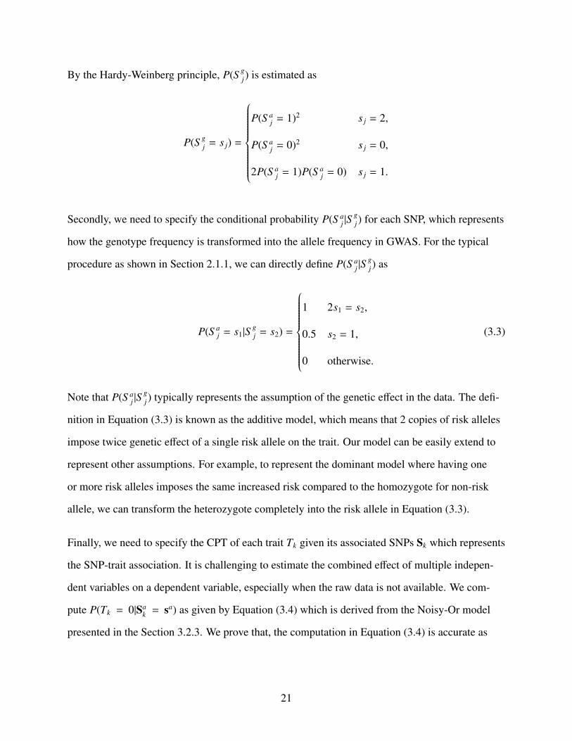
By the Hardy-Weinberg principle, P(S gj) is estimated as

P(S gj = s j) =

P(S aj = 1)2 s j = 2,

P(S aj = 0)2 s j = 0,

2P(S aj = 1)P(S a

j = 0) s j = 1.

Secondly, we need to specify the conditional probability P(S aj |S

gj) for each SNP, which represents

how the genotype frequency is transformed into the allele frequency in GWAS. For the typical

procedure as shown in Section 2.1.1, we can directly define P(S aj |S

gj) as

P(S aj = s1|S

gj = s2) =

1 2s1 = s2,

0.5 s2 = 1,

0 otherwise.

(3.3)

Note that P(S aj |S

gj) typically represents the assumption of the genetic effect in the data. The defi-

nition in Equation (3.3) is known as the additive model, which means that 2 copies of risk alleles

impose twice genetic effect of a single risk allele on the trait. Our model can be easily extend to

represent other assumptions. For example, to represent the dominant model where having one

or more risk alleles imposes the same increased risk compared to the homozygote for non-risk

allele, we can transform the heterozygote completely into the risk allele in Equation (3.3).

Finally, we need to specify the CPT of each trait Tk given its associated SNPs Sk which represents

the SNP-trait association. It is challenging to estimate the combined effect of multiple indepen-

dent variables on a dependent variable, especially when the raw data is not available. We com-

pute P(Tk = 0|Sak = sa) as given by Equation (3.4) which is derived from the Noisy-Or model

presented in the Section 3.2.3. We prove that, the computation in Equation (3.4) is accurate as

21

long as the genotype profile follows the Noisy-Or model.

P(Tk = 0|Sak = sa) =

P(Tk = 0)∏

S k j∈SkP(S a

k j = saj |T = 0)∏

S k j∈Sk

∑S g

k jP(sg

k j)P(sak j|s

gk j)

. (3.4)

As can be seen, the knowledge required for accomplish all above specifications only includes: 1)

conditional probability P(S a|T ), and 2) prior probability P(T ). The former can be estimated from

the allele frequencies f t(·) and f c(·) according to the maximum likelihood estimate, and the latter

can be acquired from literature or internet.

3.2.3. Modeling SNP-Trait Associations

This subsection derives the CPT specification formulation shown in Equation (3.4). Specifically,

given a trait T and its associated SNP S, we assume that a Noisy-Or model holds for conditional

probability of T given S’s genotype Sg, i.e., P(T |Sg). This assumption will later be empirically

validated using raw genotype data. Then, we derive Equation (3.4) from the obtained model.

Lemma 1. Let P(T |Sg) follow the Noisy-Or model. Then for Sg we have

P(Sg = s|T = 0) =

m∏j=1

P(S gj = s j|T = 0).

Proof. Conditional probability P(Sg = s|T = 0) can be written as

P(Sg = s|T = 0) =P(Sg = s)P(T = 0)

P(T = 0|Sg = s)

=

∏mj=1 P(S g

j = s j)

P(T = 0)P(T = 0|Sg = s),

P(S gj = s j|T = 0) =

P(S gj = s j)

P(T = 0)P(T = 0|S g

j = s j).

Thus we haveP(Sg = s|T = 0)∏m

j=1 P(S gj = s j|T = 0)

=P(T = 0|Sg = s)P(T = 0)m−1∏m

j=1 P(T = 0|S gj = s j)

. (3.5)

22

According to the formula of total probability and the formulation of the Noisy-Or model (2.4),

we have

P(T = 0) =∑

s

P(Sg = s)P(T = 0|Sg = s)

=∑

s

(θ0

m∏j=1

P(S gj = s j)θ

1(s j)j

)= θ0

m∏j=1

(∑s j

P(S gj = s j)θ

1(s j)j

),

and similarly

P(T = 0|S gj = s j) = θ0

∑s\{s j}

(∏i, j

P(S gi = si)P(T = 0|Sg = s)

)= θ0θ

1(s j)j

∏i, j

(∑si

P(S gi = si)θ

1(si)i

).

Then, it follows that

P(T = 0)m∏mj=1 P(T = 0|S g

j = s j)=

m∏j=1

∑s j

P(S gj = s j)θ

1(s j)j

θ1(s j)j

=θ0

∏mj=1

∑s j

P(S gj = s j)θ

1(s j)j

θ0∏m

j=1 θ1(s j)j

=P(T = 0)

P(T = 0|Sg = s),

which indicates that Equation (3.5) equals 1. Hence, the lemma is proved. �

Lemma 2. Let P(T |Sg) follows the Noisy-Or model. Then for Sa we also have

P(Sa = s|T = 0) =

m∏j=1

P(S aj = s j|T = 0).

Proof. We first derive the relationship between P(Sa = s|T = 0) and P(Sg = s|T = 0). For each

SNP S j ∈ S, suppose that the contingency table is as shown in Table 2.2. Then, the risk allele

frequency in the case group is given by

2r0 + r1

2R= r0 +

12

r1.

23

Similarly we can compute other allele frequencies. In general, the connection between the allele

frequency and the genotype frequency is given in Equation (3.6), where s = {0, 1} and t = {0, 1}.

P(S aj = s|T = t) = P(S g

j = 2s|T = t) +12

P(S gj = 1|T = t). (3.6)

We extend this equation to a combination of multiple SNPs. Given an allele combination, if a

genotype combination contains the corresponding homozygotes only, its contribution to the al-

lele frequency is 1. If there are j heterozygotes in the genotype combination, the contribution to

the allele frequency is 12 j . To obtain the general formulation, given an allele combination s (e.g.,

(A,T)), we denote the genotype combination that contains the corresponding homozygotes only

as 2s (e.g., (AA,TT)). We consider all of the possible genotype combinations that replace j ho-

mozygotes in 2s with heterozygotes, and denote this set by π j(2s). Note that π0(2s) = 2s. Thus,

the allele frequency of s is given by

P(Sa = s|T = t) =

m∑j=0

12 j

∑s′∈π j(2s)

P(Sg = s′|T = t).

According to Equation (3.6), we have

m∏j=1

P(S aj = s j|T = 0)

=

m∏j=1

(P(S g

j = 2s j|T = 0) +12

P(S gj = 1|T = 0)

)=

m∑j=0

12 j

∑s′∈π j(2s)

∏s′j∈s′

P(S gj = s′j|T = 0).

According to Lemma 1,

P(Sg = s′|T = 0) =∏s′j∈s′

P(S gj = s′j|T = 0).

24

Combining the above three equations, we have

P(Sa = s|T = 0) =

m∏j=1

P(S aj = s j|T = 0).

�

Theorem 1. Let P(T |Sg) follow the Noisy-Or model. Then we have

P(T = 0|Sa = s) =P(T = 0)

∏mj=1 P(S a

j = s j|T = 0)∏mj=1 P(S a

j = s j).

Proof. It directly follows Lemma 2 that

P(T = 0|Sa = s) =P(T = 0)P(Sa = s|T = 0)

P(Sa = s)

=P(T = 0)

∏mj=1 P(S a

j = s j|T = 0)∏mj=1 P(S a

j = s j)

=P(T = 0)

∏mj=1 P(S a

j = s j|T = 0)∏mj=1

∑S g

jP(sg

j)P(saj |s

gj)

.

�

3.3. Inference Based on the Constructed Bayesian Network

With the three-layered Bayesian network constructed from the GWAS catalog, we can calculate

the joint probability for any desired assignment of values to variable sets Sg of SNPs S and traits

T, which reflects the relationship among genotypes and traits. We first develop the general for-

mula for any inference on the constructed Bayesian network. Then we consider three specific

inference problems, namely trait inference given SNP genotype, genotype inference given trait,

and trait inference given trait. Finally, we present a typical application using the derived inference

methods.

25

3.3.1. General Inference Formula

Theorem 2. The joint probability for any value assignment to Sg of S ⊆ S, T ⊆ T , i.e., P(sg, t), is

given by

P(sg, t) =∏

S j∈S1

P(sgj)

∑Sa

2,Sg3,S

a3

( ∏S j∈S2∪S3

P(sgj)P(sa

j |sgj)

∏Tk∈T

P(tk|Par(Tk))),

where S1 denotes the SNPs in S but not associated with T, S2 denotes the SNPs in S and also as-

sociated with T, S3 denotes the SNPs associated with T but not in S. Note that∑

X f (x) means to

sum up all f (x) going through all value assignments to attributes X.

Proof. The joint probability can be written as

P(sg, t) =∑

Sa,Sg,Sa,T

P(sg, sg, sa, sa, t, t),

where S = S\S and T = T\T.

According to the Markov property, the joint probability can be factorized as

P(s, t) =∑

Sa,Sg,Sa,T

( ∏S j∈S∪S

P(sgj)P(sa

j |sgj)

∏Tk∈T

P(tk|Par(Tk))∏Tl∈T

P(tl|Par(Tl))),

which follows that

P(sg, t) =∑

Sa,Sg,Sa

( ∏S j∈S∪S

P(sgj)P(sa

j |sgj)

∏Tk∈T

P(tk|Par(Tk))∑

T

∏Tl∈T

P(tl|Par(Tl)))

=∑

Sa,Sg,Sa

( ∏S j∈S∪S

P(sgj)P(sa

j |sgj)

∏Tk∈T

P(tk|Par(Tk))).

Then, we divide S into four disjoint subsets: S1 denotes the SNPs in S but not associated with T,

S2 denotes the SNPs in S and also associated with T, S3 denotes the SNPs associated with T but

not in S, and S4 denotes all the other SNPs. Thus, S = S1∪S2, S = S3∪S4, and Par(Tk) for Tk ∈ T

26

only involves SNPs in S2 and S3. It follows that

P(sg, t) =∑

Sa,Sg,Sa

( ∏S j∈S∪S3

P(sgj)P(sa

j |sgj)

∏S j∈S4

P(sgj)P(sa

j |sgj)

∏Tk∈T

P(tk|Par(Tk)))

=∑

Sa,Sg3,S

a3

( ∏S j∈S∪S3

P(sgj)P(sa

j |sgj)

∏Tk∈T

P(tk|Par(Tk))∑Sg

4,Sa4

∏S j∈S4

P(sgj)P(sa

j |sgj))

=∑

Sa,Sg3,S

a3

( ∏S j∈S∪S3

P(sgj)P(sa

j |sgj)

∏Tk∈T

P(tk|Par(Tk)))

=∑

Sa,Sg3,S

a3

( ∏S j∈S2∪S3

P(sgj)P(sa

j |sgj)

∏S j∈S1

P(sgj)P(sa

j |sgj)

∏Tk∈T

P(tk|Par(Tk)))

=∑

Sa2,S

g3,S

a3

( ∏S j∈S2∪S3

P(sgj)P(sa

j |sgj)

∏Tk∈T

P(tk|Par(Tk))∑Sa

1

∏S j∈S1

P(sgj)P(sa

j |sgj))

=∑

Sa2,S

g3,S

a3

( ∏S j∈S2∪S3

P(sgj)P(sa

j |sgj)

∏Tk∈T

P(tk|Par(Tk))∏

S j∈S1

P(sgj))

=∏

S j∈S1

P(sgj)

∑Sa

2,Sg3,S

a3

( ∏S j∈S2∪S3

P(sgj)P(sa

j |sgj)

∏Tk∈T

P(tk|Par(Tk))).

�

Note that in Theorem 2, we apply marginalization to sum out ‘irrelevant’ variables so that we do

not need to involve all variables in our summation to calculate P(sg, t). As a result, the computa-

tion only involves variables in T, S1, S2 and S3.

Additionally, we can calculate the conditional joint probability for any desired assignment of val-

ues to variable sets Sgx,Tx given the observed assignment of variable sets Sg

y ,Ty following Theo-

rem 3. Note that Sgx and Sg

y denote the set of SNP genotypes; while Tx, Ty denote the set of traits.

Theorem 3. The probability for any desired assignment of values sgx, tx to variables in Sg

x,Tx

given the (observed) assignment of values sgy , ty to variables in Sg

y ,Ty can be directly derived

P(sgx, tx|sg

y , ty) =P(sg

x, tx, sgy , ty)

P(sgy , ty)

(3.7)

where the joint probability P(sgx, tx, sg

y , ty) and P(sgy , ty) can be calculated following Theorem 2.

27

A given Bayesian network can be used to derive the posterior probability distribution of one or

more variables in the network given the values observed for other variables in the network. The-

orem 2 and Theorem 3 show the simple and brute-force formulae, which have exponential time

complexity and are not computationally tractable. Researchers have developed various efficient

exact inference algorithms that take advantage of independence relationships represented in a

Bayesian network, and stochastic approximation algorithms to estimate exact inference results

when exact inference is prohibitively time consuming [41].

3.3.2. Trait Inference Given SNP Genotype

We assume that we have been given the genotype profile of the target and aim to derive the prob-

ability that the target has a specific trait using the constructed Bayesian network. The probability

of the prevalence of a specific trait, which is retrievable from literature or internet, is used as the

prior probability that the target has the specific trait. We then calculate the posterior probability

of the target having the trait by inferring from the target’s genotypes. Formally, we represent the

genotypes of a target v as a vector, sgv = (sg

v1, sgv2, · · · , s

gvn), with each entry sg

v j denoting the geno-

type of SNP j.

Definition 1. The problem of trait inference given SNP genotype, aims to learn the posteriori

probability P(t|sgv) that the target has a specific trait T given the target’s genotype profile sg

v using

the constructed Bayesian network.

The posteriori probability P(t|sgv) can be calculated following Equation (3.7), specifically with

sgx = ∅, ty = ∅, tx = {t}, and sg

y = sgv . In Lemma 3, we show our simplified formula where the

calculation only involves SNPs that are associated with trait T .

Lemma 3. The posteriori probability P(t|sgv) can be calculated as:

P(t|sgv) =

∑Qa

( ∏S j∈Q

P(saj |s

gv j)P(t|qa)

), (3.8)

28

where Q denotes the SNPs that are associated with trait T .

Proof. Denote by Q the SNPs that are associated with trait T . We have P(t|sgv) =

P(t,sgv )

P(sgv ) and apply

Theorem 2 to compute P(t, sgv). Note that S1 = Q, S2 = Q, and S3 = ∅. Thus, we have

P(t, sgv) =

∏S j∈Q

P(sgv j)

∑Qa

( ∏S j∈Q

P(sgv j)P(sa

j |sgv j)P(t|qa)

).

Therefore, it results that

P(t|sgv) =

P(t, sgv)

P(sgv)

=

∏S j∈Q P(sg

v j)∑

Qa

(∏S j∈Q P(sg

v j)P(saj |s

gv j)P(t|qa)

)∏

S j∈S P(sgv j)

=

∏S j∈Q P(sg

v j)∏

S j∈Q P(sgv j)

∑Qa

(∏S j∈Q P(sa

j |sgv j)P(t|qa)

)∏

S j∈S P(sgv j)

=∑Qa

( ∏S j∈Q

P(saj |s

gv j)P(t|qa)

).

�

Specifically, according to Equation (3.4), we have

P(T = 0|sgv) = P(T = 0)

∑Qa

( ∏S j∈Q

P(saj |s

gv j)P(sa

j |T = 0)∑S g

jP(sg

j)P(saj |s

gj)

),

which shows how the prior probability is updated to obtain the posteriori probability. Note that

P(T = 1|sgv) = 1 − P(T = 0|sg

v) as P(T = 1|sgv) is often of interest to users.

Lemma 3 implies that, instead of conducting inference based on the whole Bayesian network G,

we can simply identify the subgraph G′ that contains all associated SNPs of the target trait T , and

then calculate the posterior probability following Equation (3.8).

Trait inference can help an individual discovers the risk of having a certain disease based on

29

his/her genotype profile. If the genotype profile of an individual has been stolen, then it intro-

duces genetic privacy concerns since the genotypes can be used to infer private trait information

of the target by attackers.

3.3.3. Genotype Inference Given Trait

In this problem, we aim to acquire the probability that an individual has specific genotypes for

a set of SNPs given his/her associated trait information, with the Bayesian network constructed.

Formally, we denote by sgi = (sg

i1, sgi2, · · · , s

gin) an arbitrary genotype profile. A subset of a target’s

trait Tv with its value assignment tv is given.

Definition 2. The problem of genotype inference given trait aims to learn the posteriori prob-

ability P(sgi |tv) that the target has a genotype profile sg

i given the target’s traits tv using the con-

structed Bayesian network.

Lemma 4. The posterior probability P(sgi |tv) is

P(sgi |tv) =

∏S j∈Q P(sg

i j)∑

Qa

(∏S j∈Q P(sg

i j)P(saj |s

gi j)

∏Tk∈Tv

P(tk|Pa(Tk)))

∑Qg,Qa

(∏S j∈Q P(sg

j)P(saj |s

gj)

∏Tk∈Tv

P(tk|Pa(Tk))) ,

where Q denotes the SNPs that are associated with traits in Tv, and P(tk|Pa(Tk) is computed ac-

cording to Equation (3.4).

Proof. We have P(sgi |tv) =

P(sgi ,tv)

P(tv) and apply Theorem 2 to compute the probabilities. For P(sgi , tv),

similar to the proof to Lemma 3, we obtain

P(sgi , tv) =

∏S j∈Q

P(sgi j)

∑Qa

( ∏S j∈Q

P(sgi j)P(sa

j |sgi j)

∏Tk∈Tv

P(tk|Pa(Tk))),

where Q denotes the SNPs that are associated with traits in Tv. For P(tv), when applying Theo-

30

rem 2, note that S = ∅ and S = Q. Thus we have

P(tv) =∑

Qg,Qa

( ∏S j∈Q

P(sgj)P(sa

j |sgj)

∏Tk∈Tv

P(tk|Pa(Tk))).

�

3.3.4. Trait Inference Given Trait

A straightforward extension to the above two inferences is that, we can also infer other trait in-

formation of the target individual. Assume that we are given some of the target’s traits tv. Then

Lemma 5 gives the probability that the target has a new trait Tnew.

Lemma 5. The probability that the target has a new trait Tnew given some of the target’s traits tv

can be derived as

P(tnew|tv) =∑Qg

P(tnew|qg)P(qg|tv),

where Q is the set of SNPs associated with tnew and tv.

The proof is straightforward by applying the d-separation criterion [43]. We can see that P(tnew|qg)

can be derived following Lemma 3, and P(qg|tv) can be derived following Lemma 4.

Figure 3.2: Identity attack

31

3.3.5. Application: Identity Attack

We present an attack that aims to infer the probability of a record in an anonymized genotype

database that belongs to a target, when some traits of the target are available. As shown in Figure

3.2, assume that an attacker has access to an anonymized genotype dataset R that contains the

target’s genotype record sgv . The attacker also knows a subset of traits tv the target has. Then the

attacker can learn the posteriori probability P(sgi == sg

v |tv) that each genotype record sgi in the

database corresponds to the target, as shown in Lemma 6. As a result, the attacker may be able to

identify the target’s record from the anonymized dataset.

Lemma 6. The posteriori probability that the genotype record sgi corresponds to the target given

his trait tv is given by

P(sgi == sg

v |tv) =P(sg

v |tv)∑|R|i=1 P(sg

i |tv).

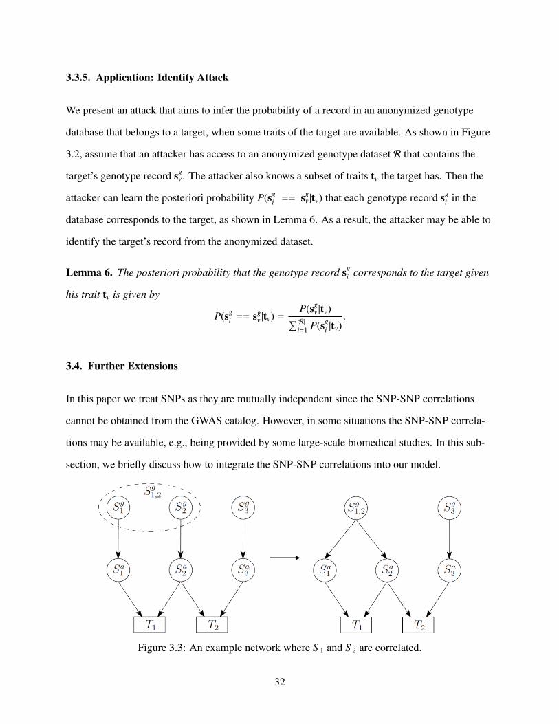
3.4. Further Extensions

In this paper we treat SNPs as they are mutually independent since the SNP-SNP correlations

cannot be obtained from the GWAS catalog. However, in some situations the SNP-SNP correla-

tions may be available, e.g., being provided by some large-scale biomedical studies. In this sub-

section, we briefly discuss how to integrate the SNP-SNP correlations into our model.

Figure 3.3: An example network where S 1 and S 2 are correlated.

32

When the SNP-SNP correlations are available, we assume that in addition to the allele frequency

in the case and control groups, we also know the joint genotype frequency of the correlated SNPs.

Then, a straightforward extension of our model can be given as follows. For two or more corre-

lated SNPs, we cluster their corresponding nodes in the genotype layer as a single super node.

The super node represents the combination of the SNP genotypes, and takes value as the cross-

product of the sets of values of the genotypes. There is an edge pointing from the super node to

each corresponding allele node. Note that the clustered Bayesian network represents the same

joint probability distribution as the original Bayesian network.

Figure 3.3 shows an example, where SNPs S 1 and S 2 are correlated. Thus, we cluster nodes

S g1, S

g2 as a single node S g

1,2, i.e., S g1,2 = S g

1 × S g2. Node S g

1,2 has two emanating edges pointing

to S a1 and S a

2 respectively. Denoting the value combination (sg1, s

g2) by sg

1,2, according to Equation

(2.3), the joint probability of P(sg1,2, s

g3, t1, t2) in the clustered Bayesian network is given by

P(sg1,2, s

g3, t1, t2) =

∑S a

1,Sa2,S

a3

P(sg1,2)P(sg

3)P(sa1|s

g1,2)P(sa

2|sg1,2)P(sa

3|sg3)P(t1|sa

1, sa2)P(t2|sa

2, sa3). (3.9)

In Equation (3.9), P(sg1,2) = P(sg

1, sg2) is assumed to be given representing the known SNP-SNP

correlation. For P(sa1|s

g1,2) (resp. P(sa

2|sg1,2)), as shown in Section 3.2.2 it represents for SNP S 1

(resp. S 2) how the genetic effect of the genotype is obtained from the genetic effects of its two al-

leles, hence has no connection with other SNPs. So, we have P(sa1|s

g1,2) = P(sa

1|sg1) and P(sa

2|sg1,2) =

P(sa1|s

g2). For P(t2|sa

2, sa3), it can be accurately computed using Theorem 1 since S g

1,2 and S g3 are in-

dependent. The only issue of exactly computing Equation (3.9) lies in the computing of P(t1|sa1, s

a2).

Since P(t1|sa1, s

a2) can be written as P(t1)

P(sa1,s

a2) P(sa

1, sa2|t1), and we can easily obtain that P(sa

1, sa2) =∑

S g1,2

P(sa1|s

g1)P(sa

2|sg2)P(sg

1,2), we focus on the computing of P(sa1, s

a2|t1).

If P(sa1, s

a2|t1) is also given, then Equation (3.9) can be exactly computed. If not, we can estimate

33

P(sa1, s

a2|t1) as follows. We have

P(sa1, s

a2) − P(sa

1)P(sa2) =

∑T1

P(sa1, s

a2|t1)P(t1) −

∑T1

P(sa1|t1)P(t1)

∑T1

P(sa2|t1)P(t1).

Usually, P(T1 = 0) is much larger than P(T1 = 1). Thus, by approximating P(T1=1)P(T1=0) and P(T1=1)

√P(T1=0)

by

zero, it follows that

P(sa1, s

a2) − P(sa

1)P(sa2) ≈ P(T1 =0)

(P(sa

1, sa2|T1 =0) − P(sa

1|T1 =0)P(sa2|T1 =0)P(T1 =0)

),

which leads to

P(sa1, s

a2|T1 = 0) ≈

P(sa1, s

a2) − P(sa

1)P(sa2)

P(T1 = 0)+ P(sa

1|T1 = 0)P(sa2|T1 = 0)P(T1 = 0).

It should be noted that, the above extension cannot deal with the situation where the SNP-SNP

correlations have overlaps, e.g., in Figure 3.3 S 2 is correlated with both S 1 and S 3 but the correla-

tion among the three SNPs are not available. In this case, we can resort to the factor graph model

[32] to represent the SNP-SNP correlations. We leave the detailed study to the future work.

3.5. Experiments

We first validate the Noisy-Or model in Section 3.5.1. Then we construct the Bayesian network

from the GWAS catalog in Section 3.5.2. The inference methods and their applications are evalu-

ated in Sections 3.5.3 and 3.5.4.

3.5.1. Noisy-Or Model Validation

To evaluate the fitness of the Noisy-Or model in modeling the SNP-trait association, we use raw

data from openSNP [10] where more than two thousand users over the world share their genotype

profiles and trait information. The genotype file contains the results of the genetic test taken by

34

each user. Each line in the file corresponds to one SNP with its identifier (rsid), its location on the

reference human genome and alleles provided. Besides, users also contribute their phenotypes to

openSNP, such as what the color of their eyes, whether they have astigmatism, or whether they

are suffering from irritable bowel syndrome.

Data Setup

In the experiments, we use openSNP of version 20151231. The genetic test results provided by

users are taken from different genetic screening services. We focus on the genotyping files from

23andMe, Ancestry and FamilyTreeDNA. The data from these services account for more than

99% of the whole dataset. Among the 341 traits from the original data, there are 129 binary traits,

136 non-binary categorical traits, 39 numeric traits and 14 traits with unknown values. In align

with GWAS case-control settings, we focus on the 129 binary traits to evaluate our models.

The data in openSNP is highly sparse and contains a mass of missing values due to various ge-

netic testing platforms and varying willingness of individuals to share their traits. To ensure that

the statistic tests in the model construction are meaningful, we further filter the data as follows.

For each trait, we extract the individuals that belong to the control group and the case group. If

the number of individuals contained in both groups for a trait is less than 10, we exclude this trait

from our experiment. As a result, we obtain 71 traits satisfying the requirement. Then, follow-

ing a typical GWAS procedure [52], from all associated SNPs for each trait, we remove the SNPs

with: 1) low minor allele frequency (i.e., <1%); 2) call rate less than 90%; and 3) the number of

records containing the risk allele less than 10. After that, we discard the traits with no associated

SNPs left after filtering. Finally, we obtain a dataset which contains 23 traits and 256,845 SNPs.

Results

To build the Bayesian network, we extract for each trait the associated SNPs along with risk al-

lele types, risk allele frequencies and odds ratios. For each SNP, the allele frequencies in the case

group and the control group and odds ratios are computed. If the odds ratio is larger than 1, the

35

Table 3.1: SNP-Trait associations

Traits SNPs Traits SNPs

Eye with Blue Halo rs6913354 Irritable Bowel Syndrome rs8039023rs10460585 rs2948814

Hair on Fingersrs1239925

Do You Grind Your Teeth

rs3923767rs11715867 rs2531864rs2302025 rs2042279

ADHD

rs1496496 rs12094507rs4619 rs9809185rs7235392

Enjoy Driving A Car

rs2409764rs664510 rs12564559rs1910236 rs10882959rs6922476 rs6601522

Astigmatism

rs747644 rs1002399rs1466410 rs6993841rs11680053 rs958648rs12358733 rs3808513rs1400390 rs6601518rs10508470 rs357281

corresponding allele is considered as the risk allele. Then, we perform the Fisher’s exact test of

independence to test whether the association between the trait and the SNP is significant. The

threshold of the p-value is set as 4 × 10−5. We discard the traits with zero associated SNP, as well

as the traits with only one associated SNP as they have no effect in testing ICI model. As a result,

we obtain 7 traits and 34 associated SNPs for building the Bayesian network, as shown in Table

3.1.

Table 3.2: The chi-square value, degree of freedom (df), p-value, RMSEA of the Noisy-or model

Trait Chi-square df p-Value RMSEAEye with Blue Halo 6.73 4 0.15 0.10Hair on Fingers 14.46 14 0.41 0.02Irritable Bowel Syndrome 5.24 4 0.26 0.05ADHD 55.32 53 0.38 0.02Astigmatism 132.55 123 0.26 0.02Do You Grind Your Teeth 50.13 49 0.42 0.02Enjoy Driving A Car 96.33 98 0.52 NA

We then evaluate the fitness of the Noisy-Or model. For each trait, we predict the observed num-

ber of individuals with a specific trait and specific SNP genotypes, i.e., n(T,Sg), by computing

the predicted value as n(T,Sg) = P(T |Sg)n(Sg), where n(Sg) is the observed total number of indi-

viduals with the SNP genotypes. Since the data is highly sparse, when computing the chi-square

36

value we only sum up the cells where n(Sg) does not equal to 0. We then compute the p-value to

show the significance. The degree of freedom is computed as “total number of predictions - the

number of non-zero n(Sg) - the number of model parameters”. The null hypothesis H0 assumes

that there is no relationship between the data and the model. Thus, the model is not rejected if

p-value >0.05. In addition, we further compute the Root Mean Square Error of Approximation

(RMSEA) values [34] which is an absolute measure of fit, to show the degree of the fitness. The

RMSEA values are categorized into four levels: close fit (.00 - .05), fair fit (.05 - .08), mediocre

fit (.08-.10) and poor fit (over .10). Note that RMSEA is applicable only when the chi-square

value is larger than the degree of freedom (df), and is labelled as ‘NA’ otherwise. The results are

shown in Table 3.2. As can be seen, the Noisy-Or model is accepted for all traits according to the

p-values, which indicates the model is a good fit. The values of RMSEA show a close fit in gen-

eral. Therefore, we validate the use of the Noisy-Or model in modeling SNP-trait association.

3.5.2. Bayesian Network Construction

With the justified Noisy-Or model for constructing a Bayesian network, we set out to construct

a Bayesian network captured in GWAS statistics. Specifically, we construct a Bayesian network

using data extracted from the online GWAS catalog [57] as of Feb 25th, 2016. This version of

the GWAS catalog includes 2,347 publications and 23,152 records (SNP-trait pairs) about 17,781

SNPs associated with 1,457 traits. Publications included in such a catalog are limited to those

attempted to assay at least 100,000 SNPs in the initial stage. SNP-trait pairs listed are limited

to those with p-values less than 10−5. For each record, the odds ratio or beta coefficient is pro-

vided to indicate the association of the trait-SNP pair, depending on whether the trait is categori-

cal (e.g., some disease) or numerical (e.g., height). The two values are contained in the same field

in the dataset.

In this chapter, we target for categorical variables only. Thus, we focus on a subset of data pub-

lished as the interactive diagram by the GWAS catalog, where an additional attribute “orType”

is used to clearly indicate whether the odds ratio is provided. This subset of data includes 5,047

37

records with 791 traits associated with 4,250 SNPs, and SNP-trait pairs are limited to those with

p-values less than 5 × 10−8. We extract the records with the odds ratio provided. As a result, we

obtain 2,325 records with 266 traits associated 2,177 SNPs. Among these SNPs, there are 1,941

SNPs associated with a single trait, 122 SNPs associated with two traits, and at the most, one

SNPs associated with 7 traits. Finally, we build a knowledge database for all extracted traits and

associated SNPs including the risk allele type, risk allele frequency in the control group, and the

odds ratio.

Based on the knowledge database, we build the Bayesian network according to Section 3.2.2.

Particularly, to acquire the prior probability (prevalence) of each trait, we classify all the traits

into 17 categories (e.g., immune system disease, nervous system disease), and retrieve the av-

erage prevalence of each category from the Wikipedia [58]. We use the average prevalence of a

category as the prior probability of each trait belonging to the category. Our constructed Bayesian

network can be refined by assigning the accurate prior probability for each trait when available.

3.5.3. Simulated Scenario: Trait Inference

We evaluate the constructed Bayesian network using two simulated scenarios. In the first sce-

nario, we infer the probability of an individual of having a trait given his/her genotype profile us-

ing the constructed Bayesian network. We use the genotype profiles in the 1000 Genomes Project

[50] and extract a dataset referred to as ‘CEU’ for our experiment. It consists of 99 HapMap in-

dividuals from Utah residents with Northern and Western European ancestry (CEU) in the 1000

Genomes Project, which are treated as targets of trait inference in this study.

For each CEU individual v, we compute his/her posterior probability P(Tk = 1|sgv) of having

each trait Tk given the SNP genotype profile sgv according to Lemma 3. Then, we compute the rel-

ative difference rd between the prior probability and the posterior probability of each trait, i.e.,

rd =P(Tk=1|sg

v )−P(Tk=1)P(Tk=1) , and rank the traits according to the rd for each individual. Figure 3.4 shows

for top-3 and bottom-3 traits of each individual. A total of 24 traits are included as illustrated in

38

Figure 3.4: Top-3 and bottom-3 traits of each CEU individual

Figure 3.4, each of which is represented as a row. Each column shows the top traits of an indi-

vidual, where the green and red dots represent the traits with the most positive and negative rd

respectively.

Table 3.3: Trait-SNP association

Index Trait SNP-risk allele f tk j(r) Ok j f c

k j(r) P(tk)

1 Type 1 diabetes rs9272346-G 0.13 8.3 0.55 0.25rs2647044-A 0.61 5.49 0.902 Behcet’s disease rs17482078-T 0.02 4.56 0.09 0.04

3 Crohn’s diseasers11924265-C 0.02 3.99 0.08

0.26rs76418789-G 0.93 2.06 0.97rs2066847-G 0.06 2.27 0.13

4 Fuchs’s corneal dystrophy rs613872-G 0.15 5.47 0.49 0.095 Freckles rs1805007-T 0.05 4.37 0.19 0.056 Celiac disease rs2187668-T 0.26 6.23 0.68 0.267 Immunoglobulin A 0.13 2.53 0.27 0.05

Tables 3.3 and 3.4 show the information of a snapshot of the constructed Bayesian network and

the computed posterior probabilities. There are 7 traits and 9 SNPs. In Table 3.3, the risk allele

type, risk allele in the control group and the odds ratio of each each SNP-trait pair are shown in

Columns 3-5. Note that SNP rs2187668 is associated with two traits. The calculated risk allele

frequency in the case group for each SNP-trait is shown in Column 6. Note that there is a big gap

between the risk allele frequency in the case group and that in the control group. The prior proba-

bility (prevalence) of each trait is shown in Column 7. In Table 3.4, each index corresponds to the

trait with the same index in Table 3.3. Columns sgv and Count respectively show the genotypes of

39

the associated SNPs and the number of individuals who have the genotypes. As before, 0 denotes

the genotype of two non-risk alleles, 2 denotes the genotype of two risk alleles, and 1 denotes the

genotype of one risk allele and one non-risk allele. Column P(t|sgv) shows the posterior proba-

bility of one individual has a trait given his SNP genotype profile. The last column rd shows the

relative difference between the prior probability and the posterior probability of each trait. As

can be seen, all the posterior probabilities are significantly different from the corresponding prior

probability of having a trait. In general, the posterior probability of a trait is larger if the indi-

vidual has more risk alleles.Hence, the constructed Bayesian network is useful to infer new trait

information. We also observe that, when there are multiple associated SNPs, the effect of each

SNP can be different. For example, Trait 1 is associated with two SNPs. The posterior probability

when the genotypes are (0, 1) is larger than that when the genotypes are (2, 0), implying that the

second SNP has greater effect than the first one.

Table 3.4: Posterior probability of certain trait considering associated SNPs

Index sgv Count P(t|sg

v) rd Index sgv Count P(t|sg

v) rd

1

(0,0) 28 0.149 -0.4033

(0,2,2) 89 0.349 0.341(1,0) 30 0.198 -0.208 (1,2,2) 7 0.367 0.411(2,0) 22 0.247 -0.012 (2,2,2) 3 0.385 0.481(0,1) 10 0.269 0.078

4(0) 66 0.056 -0.379

(1,1) 6 0.311 0.245 (1) 27 0.150 0.670(2,1) 3 0.353 0.413 (2) 6 0.245 1.718

2(0) 55 0.037 -0.064

5(0) 75 0.043 -0.138

(1) 36 0.094 1.351 (1) 23 0.104 1.076(2) 8 0.151 2.766 (2) 1 0.164 2.289

6 (0) 80 0.129 -0.501 7 (0) 80 0.024 -0.511(1) 19 0.305 0.174 (1) 19 0.108 1.162

3.5.4. Simulated Scenario: Identity Inference

In this scenario, we evaluate whether a target individual can be identified from an anonymized

genotype database by an attacker given some traits of the target individual using the Bayesian

network. For comparison we also include Humbert’s de-anonymizing method proposed in [20].

This method also aims to identify the genotypes that correspond to the given traits, making use of

the single SNP-single trait correlation. The difference lies in that this method rely upon some in-

validated independence assumption, whereas our method is based on the independence of causal

40

influence, which is shown to have good fitness in modeling the SNP-trait associations in Section

6.1. We compare the identification accuracy of the Humbert’s method to our method.

Table 3.5: Trait-SNP pairs

Trait SNP-risk allele Ok j

Exfoliation glaucoma rs893818-A 20.94rs3825942-G 20.1

Response to hepatitis C treatmentrs11697186-A 33.33rs8099917-G 27.1rs6139030-T 25

Blue vs. brown eyes rs1667394-T 29.43Skin pigmentation rs1834640-G 12.5

We consider the 7 trait-SNPs pairs listed in Table 3.5 whose odds ratios are larger than 10. The

’CEU’ dataset is used to serve as the anonymized genotype database. To simulate an attack, we

first designate a target individual whose traits tv and genotypes sgv are known. Then we blend the

genotype profile of the target into the ’CEU’ dataset (containing the genotype records of the 99

unrelated CEU individuals), and attempt to re-identify it assuming that the attacker only knows

the target’s traits tv. To define the target, we assume that the target has all the traits, i.e., the target

has Tk = 1 for each trait Tk. We then randomly generate the genotype record for the target indi-

vidual. The generating strategy is that for each SNP S k j associated with one trait Tk, we generate

S gk j = sg

k j with the probability P(S gk j = sg

k j|Tk = 1). In this way we simulate a scenario where

the target is randomly selected from the case group characterized by GWAS statistics. Finally, we

calculate the probability that the generated record is correctly identified as belonging to the tar-

get individual, given the background trait information, according to Lemma 6. We also compare

the identification capability with different amount of background knowledge, i.e., with the size of

trait set tv ranging from one to four.

We run this whole process 10,000 times for each trait set. Figure 3.5a shows the average value of

the resulted probabilities. As shown in Figure 3.5a, the green line is the baseline representing the

probability 1/100 (100 = 99 ‘CEU’ individuals + 1 target) that the generated record is inferred as

belonging to the target individual without any background knowledge. The blue line represents

the inferred probability based on the Bayesian network, and the red line represents the inferred

41

(a) (b)

Figure 3.5: (a) Average Probability of Identification; (b) Probability Distribution of Identification

probability using the Humbert’s method. The first points in the blue and red lines represent the

results given the first trait (according to the trait index in Table 3.5) of the target. Similarly, the

second points represent the results given both the first two traits of the target, and so on. The bar

at each point shows the standard deviation of the resulting probabilities of 10,000 times of test.

We can see that in general, the probabilities of correctly identifying the target individual of both

methods increase as the background knowledge increases, and the identification probability our

method is significantly larger than that of the situation without any background knowledge (i.e.,

0.01). Comparing the two methods, our method consistently outperforms the Humbert’s method

(the p-value of the t-test is 0.005). In addition, the identification probability given only one trait

of our method is even larger than that given all four traits of the Humbert’s method, showing that

our method significantly improves the identification accuracy over the Humbert’s method.

Figure 3.5b shows the distribution of the inference probability among the 10,000 times of iden-

tifications of our method. As the amount of background traits increases, the peaks of the process

count would be located at positions with larger identifying probabilities. This indicates that in

general, the more background knowledge we have, the more probably that the target individual’s

record is correctly identified. On the other hand, multiple peaks in each line represent different

identifying probabilities due to different combinations of background traits, as well as different

42

possible genotype records being randomly generated.

As an alternative method of defining the target, we leverage the openSNP users as they share both

of their trait and genotype profiles online. By blending the profile of an openSNP user into the

’CEU’ dataset and re-identifying it, we evaluate the risk of privacy leak of the openSNP users

although their profiles are anonymized. One issue here is that the sets of traits and SNPs con-

tained in the GWAS catalog and those contained in openSNP are not identical. In order to per-

form the attack, we select the target individuals from openSNP who have reported the traits and

SNPs which are also contained in the GWAS catalog. Thus, we first identify the overlapped traits

and SNPs contained in both the GWAS catalog and openSNP. Among all the identified traits and

SNPs, we further require that the odds ratio of the trait-SNP pair to be larger than 2 so that the

effect of the SNP on the trait is significant. We have 3 traits and 7 associated SNPs satisfying

the requirement, which are shown in Table 3.6. Then, we select the openSNP users who have

reported at least one of the three traits and all the SNPs associated with the reported traits. As a

result, we obtain a total of 101 openSNP users who are considered as targets in the experiment.

Table 3.6: Trait-SNP association

Index Trait SNP-risk allele f tk j(r) Ok j f c

k j(r) P(tk)

1 Rheumatoid arthritis rs6457617-T 0.49 2.36 0.69 0.01rs9275406-T 0.17 2.1 0.302 Hypertriglyceridemia rs964184-G 0.14 3.28 0.35 0.30

3 Multiple sclerosis

rs3129889-G 0.2 2.97 0.43

0.01rs3129934-T 0.1 2.34 0.21rs3135388-A 0.22 2.75 0.44rs9271366-G 0.15 2.78 0.33

We compute the probability for each target to be correctly identified from the database. The re-

sults for all targets are shown in Figure 3.6a. As can be seen, nearly half (51/101 for our method

and 41/101 for the Humbert’s method) of the targets have the probability of identification higher

than 0.01. In this case, it shows that there is no obvious risk for openSNP users. This is probably

due to the difference between the openSNP users and the population represented by the GWAS

catalog. However, as shown in Figure 3.6b, if we confine the targets to those who have at least re-

ported the trait of “Hypertriglyceridemia”, they have higher chances to be more accurately iden-

43

(a)(b)

Figure 3.6: Probability of identification: (a) all targets; (b) targets with hypertriglyceridemia

tified (19/30 for our method and 13/30 for the Humbert’s method). These results show that, for

certain openSNP users there are higher risk of privacy leak. Under what circumstance the open-

SNP users may face higher risk of privacy leak is worthy of further study. Comparing the two

methods, it can be seen that our method still outperforms the Humbert’s method in term of the

identification accuracy.

3.6. Related Work

The detection of SNP-trait associations by building Bayesian networks has been studied in biomed-

ical fields, where a Bayesian network is used to address the high computationally complex and

high dimensional problems. In [24] the authors used a score-based Bayesian network structure

learning algorithm to detect epistasis or interactions among SNPs. In [12], the same problem

is addressed by using a new information-based score and a branch-and-bound search algorithm

to discover the structure of the Bayesian network. As an extension to the work of [24], a recent

study [60] proposed an exhaustive search on a Bayesian network to detect high order associations

of SNPs with traits, without requiring marginal effects on low dimensional datasets. All of the re-

lated work aforementioned requires a raw genotype dataset to construct a Bayesian network. Our

work is novel in that we build a Bayesian network from the publicly released GWAS statistics

where the underlying genotypes are not publicly available.

44

Our method is based on the models of Independence of Causal Influence. ICI is proposed to

overcome the problem of specifying a large number of conditional probability distributions in

the CPT for a node with multiple parents in the Bayesian network. Examples of widely used

ICI models include Noisy-Or, Noisy-Max, Linear-Gaussian, etc. [16]. The Noisy-Max model

is equivalent to the Noisy-Or model in our situation where each hidden variable X j is binary. The

Linear-Gaussian model is proposed for modeling numeric variables. Therefore, these two models

are not discussed in this chapter.

Genetic privacy has also been actively studied in the literature (refer to survey papers [7, 39,

48]). For example, Homer et al. developed a method that can identify whether a target with some

known SNPs comes from a population with known allele frequency [18]. It attracted more and

more attention on the privacy disclosure of the public dissemination of the genotype-related data

and aggregate statistics from the genome-wide association studies (GWAS) [21, 36, 46, 47, 53,

55, 64]. Another work [11] showed that full identities of personal genomes can be exposed via

surname inference from recreational genetic genealogy databases followed by Internet searches.

They considered a scenario in which the genomic data are available with the target’s year of birth

and state of residency, two identifiers that are not protected by HIPAA. In our previous work [56],

we also studied whether and to what extent the unperturbed GWAS statistics can be exploited

by attackers to breach the privacy of regular individuals who are not GWAS participants. Two

attacks, namely trait inference attack and identify inference attack were formalized based on

the 2-layer Bayesian network inference and empirically evaluated. In [49], the authors devel-

oped a likelihood-ratio test that uses allele presence or absence responses from a Web service

called beacon to derive whether a target individual genome is present in the database. In [45],

the authors proposed practical strategies including obscuration and access control for reducing

re-identification risks in beacons. In [20], the authors studied the use of phenotypic traits to re-

identify users in anonymized genomic databases such as OpenSNP and 23andMe and demon-

strated that the privacy risks due to genotype-phenotype associations. In [19], the authors pro-

posed to build a Bayesian network to represent the genotype and phenotype dependencies among

45

family members, so that the genotype of a family member can be inferred from the genotypes and

phenotypes of his relatives. When the correlation among genotypes are considered, the authors

further adopted the factor graph instead of the Bayesian network to represent the familial depen-

dencies.

Several research works [8, 25] have been conducted for the safe release of aggregate GWAS

statistics without compromising a participant’s privacy. Their ideas were based on differential pri-

vacy [5]. Differential privacy is defined as a paradigm of post-processing the output and provides

guarantees against arbitrary attacks. A differentially private algorithm provides an assurance that

the output cannot be exploited by the attacker to derive whether or not any individual’s record is

included. The privacy parameter ε controls the amount by which the distributions induced by two

neighboring data sets may differ (smaller values enforce a stronger privacy guarantee). A general

method for achieving differential privacy for a query f is to compute the sum of the true output

and random noise generated from a Laplace distribution. The magnitude of the noise distribu-

tion is determined by the sensitivity of the query and the privacy parameter specified by the data

owner. The sensitivity of a computation bounds the possible change in the computation output

over any two neighboring data sets (differing at most one record). For example, the sensitivity

values of chi-square statistic and p-value were derived in [8]. For those statistics with large sen-

sitivity values (e.g., the sensitivity of odds ratio is infinity), the authors in [8] adapted the idea of

releasing the most significant patterns together with their frequencies in the context of frequent

pattern mining [1] to release K most significant SNPs. In [25], the authors developed distance-

score based privacy preserving algorithms for computing the number and location of SNPs that

are significantly associated with the trait, the significance of any statistical test between a given

SNP and the trait, correlation between SNPs, and the block structure of correlations. In [51], the

authors developed methods for releasing differentially private χ2-statistics in GWAS while guar-

anteeing membership privacy in adversarial settings [30].

46

3.7. Summary

In this chapter, we first studied the construction of Bayesian networks from publicly released

GWAS catalog. We employed the models of independence of causal influences (ICI) which as-

sume that the causal mechanism of each parent variable is mutually independent. We derived a

formulation from the Noisy-Or model, one of the ICI models, to specify the CPT using GWAS

statistics, and developed a Bayesian Network construction algorithm based on the CPT spec-

ification formulation. We proved that, the specified CPT is accurate as long as the underlying

individual-level genotype and phenotype profile data follows the Noisy-Or model. In the exper-

iments, we empirically validated the fitness of the Noisy-Or model. Then, we developed three

inference problems based on the constructed Bayesian network, namely trait inference given SNP

genotype, genotype inference given trait, and trait inference given trait. We developed efficient

formulas and algorithms to infer posterior probabilities. Finally, we empirically evaluated the de-

rived inference methods for two applications. In the first application, we showed that significant

amount of knowledge regarding traits can be inferred from the genotype profiles. In the second

application, we showed that the probability of an individual to be identified from an anonymized

genotype database is increasing given some traits of the individual.

Part of the work in this chapter is published in the Proceedings of the 2016 IEEE International

Conference on Bioinformatics and Biomedicine [63] and IEEE/ACM Transactions on Computa-

tional Biology and Bioinformatics [62].

47

4. Modeling SNP and Quantitative Trait Association Using CLG Bayesian Network

4.1. Introduction

In Chapter 3, we introduce a traditional Bayesian network to deal with the categorical traits. In

the GWAS catalog, more than half of the traits are quantitative. The association between SNPs

and these quantitative traits cannot be modeled using the previous method due to the mixture of

discrete (SNPs and categorical traits) and continuous (quantitative traits) variables.

In this chapter, we address this problem by leveraging the Conditional Linear Gaussian (CLG)

Bayesian network [27]. In a CLG Bayesian network, the variables are partitioned into two sets,

a set of discrete variables and a set of continuous variables. For each discrete variable, it is as-

sociated with a CPT similar to the traditional Bayesian network. For each continuous variable,

there is a CLG distribution conditional on each value assignment of its parents. We proposed the

method to build the CLG Bayesian network from the GWAS catalog, focusing on the specifi-

cation of the CLG distribution for quantitative traits. We then develop efficient inference meth-

ods based on the constructed network. For simplicity, we only consider quantitative traits in this

chapter, but our model can be easily extended to the mixture of categorical and quantitative traits.

We discuss the extensions of our model in Section 4.4.

We empirically evaluate the construction and inference methods. We show that useful informa-

tion regarding the traits and SNPs can be inferred using the constructed network. A case study

is also performed to evaluate how much individual information can be disclosed. This can help

evaluate the potential risk due to the statistics released in GWAS catalog [20, 56]. We assume an

anonymized genotype profile database and a target whose genotype profile is known to be con-

tained in the database. An attacker knows some of traits of the target and aims to identify the tar-

get’s record from the database. The results show that the attacker can increase his success likeli-

hood by exploiting the traits of the target.

The rest of this chapter is organized as follows. Section 4.2 describes the construction of the CLG

48

Bayesian network from the GWAS catalog. Followed by that, Section 4.3 presents the inference

methods based on the constructed network, and Section 4.4 presents several extensions. The ex-

perimental setup and results are discussed in Section 4.5. Section 4.6 summarizes the related

work and Section 4.7 concludes this chapter.

4.2. Learning CLG Bayesian Network from GWAS Statistics

In this section, we study the construction of a CLG Bayesian network from the GWAS catalog to

model the SNP-quantitative trait association. We first identify the statistical knowledge that can

be extracted and derived from the GWAS catalog. Then we show how to learn the CLG Bayesian

network using the acquired statistics only. The challenge is to specify all parameters of the CLG

distributions as shown in Equation (2.5) without access to the raw data. We make use of the as-

sumption of ICI to facilitate the specification. The ICI assumption has already been shown to

have good fitness in modeling SNP-trait associations [63]. Finally, we develop the methods to

completely specify the CLG Bayesian network.

4.2.1. Knowledge from GWAS catalog

Consider a set of traits T and a set of SNPs S in the GWAS catalog. Each trait T ∈ T is a con-

tinuous variable whose mean is denoted by µ and variance is denoted by σ2. Assume that the trait

is identified to be associated with a subset of m SNPs S = {S 1, · · · , S m} ⊆ S. For each SNP

S i ∈ S, denote its genotype as si = {0, 1, 2}, where 0 represents two non-risk alleles, 1 repre-

sents one non-risk allele and one risk allele, and 2 represents two risk alleles. The association test

for trait T and SNP S i is performed over a simple of n individuals by fitting the linear regression

t = β0 + βsi + ε. The values of n, β and the p-value of the ANOVA can be directly extracted from

the GWAS catalog.

In addition to the above directly released statistics, we can also derive variance σ2 and parame-

ter β0, assuming that the values of mean µ and the population genotype frequency P(si) can be

acquired from the literature or Internet, as shown in Lemma 7.

49

Lemma 7. The values of variance σ2 and intercept β0 can be derived as

β0 = µ − β∑

si={0,1,2}

P(si)si,

σ2 =(n−2+F∗)

(n0(β0−µ)2 + n1(β0+β1−µ)2 + n2(β0+2β1−µ)2

)nF∗

.

Proof. Straightforwardly we have the following estimation

µ = E[T ] =∑

si={0,1,2}

p(si)t =∑

si={0,1,2}

p(si)(β0 + βsi).

Thus, β0 can be derived as

β0 = µ − β∑

si={0,1,2}

p(si)si.

On the other hand, since the p-value is obtained through an F-test, ratio F∗ can be recovered us-

ing the p-value and the F(1, n − 1) distribution. According to definition of SSR, we have

SSR =

n∑k=1

(tk − µ)2 = n0(β0 − µ)2 + n1(β0 + β1 − µ)2 + n2(β0 + 2β1 − µ)2,

where nsi = np(si) is the number of individuals with genotype si. Since F∗ = SSR/1SSE/(n−2) , we have

SSE = (n − 2)SSRF∗ . Meanwhile, the total sum of squares (SSTO) is defined as

SSTO =

n∑k=1

(tk − µ)2,

which can be estimated by nσ2. In ANOVA, we have

SSTO = SSR + SSE.

50

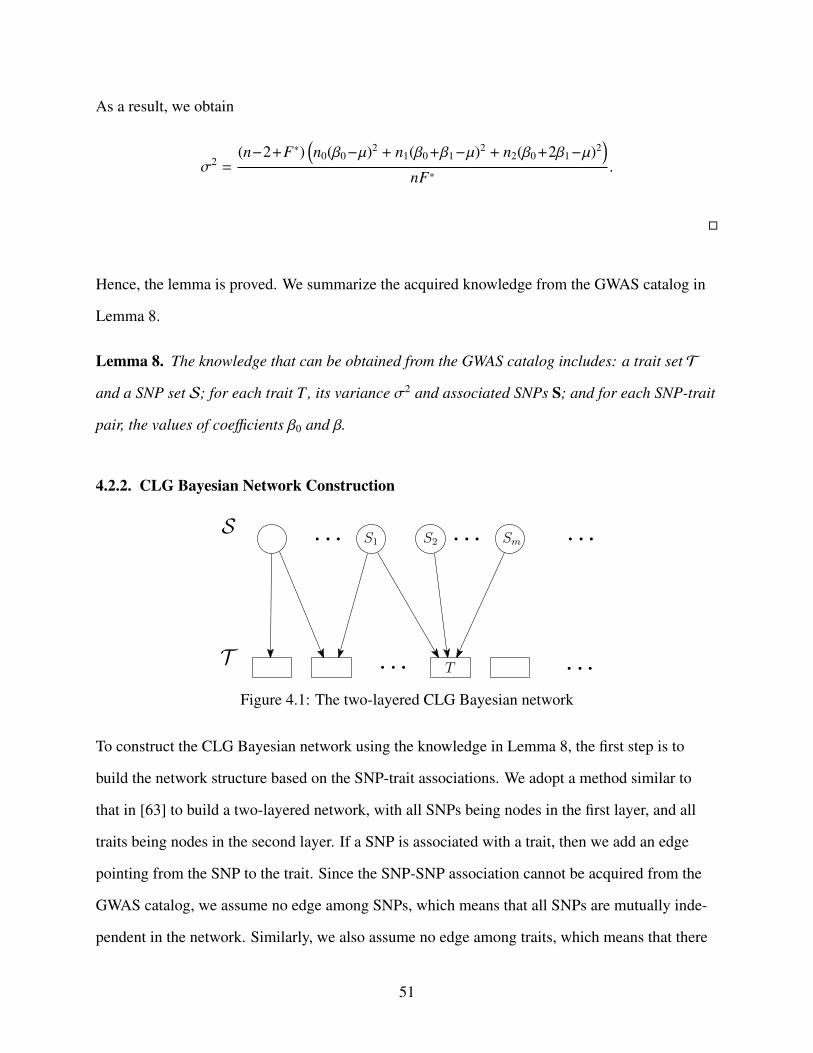
As a result, we obtain

σ2 =(n−2+F∗)

(n0(β0−µ)2 + n1(β0+β1−µ)2 + n2(β0+2β1−µ)2

)nF∗

.

�

Hence, the lemma is proved. We summarize the acquired knowledge from the GWAS catalog in

Lemma 8.

Lemma 8. The knowledge that can be obtained from the GWAS catalog includes: a trait set T

and a SNP set S; for each trait T , its variance σ2 and associated SNPs S; and for each SNP-trait

pair, the values of coefficients β0 and β.

4.2.2. CLG Bayesian Network Construction

S1

T

S2 SmS

TFigure 4.1: The two-layered CLG Bayesian network

To construct the CLG Bayesian network using the knowledge in Lemma 8, the first step is to

build the network structure based on the SNP-trait associations. We adopt a method similar to

that in [63] to build a two-layered network, with all SNPs being nodes in the first layer, and all

traits being nodes in the second layer. If a SNP is associated with a trait, then we add an edge

pointing from the SNP to the trait. Since the SNP-SNP association cannot be acquired from the

GWAS catalog, we assume no edge among SNPs, which means that all SNPs are mutually inde-

pendent in the network. Similarly, we also assume no edge among traits, which means that there

51

is no direct correlation between traits. However, two traits can still be correlated via SNPs if they

share the same SNPs. We will discuss how to relax these assumptions in Section 4.4. As a result,

we obtain a special CLG Bayesian network where the continuous variables (traits) only have dis-

crete parents (SNPs). The structure of the network is illustrated in Figure 4.1.

The next step is to specify the conditional probability distribution for each SNP, and the CLG

distribution for each trait. For a SNP S , the conditional probability distribution is directly speci-

fied by the genotype frequency p(s), which can be acquired from the literature or Internet as dis-

cussed in the previous subsection. For a trait T , following Equation (2.5), the CLG distribution

given T ’s associated SNPs S is given by

P(t|s) = N(t; a(s), c(s)). (4.1)

Note that the above equation does not include parameters b(·) since the trait has no continuous

parent.

Parameters a(·) and c(·) capture the joint effect of all associated SNPs on the trait. However, the

GWAS statistics shown in Lemma 8 only provide the association between T and each of its asso-

ciated SNP. In addition, the number of parameters in a(·) and c(·) is exponential to the size of S,

making them impractical to be specified in a direct manner. Since it has already been shown in

[63] that the assumption of ICI has a good fitness in modeling the SNP-trait association, we also

adopt the ICI assumption to facilitate the parameter estimation in CLG distribution specification.

ICI assumes that, when there are multiple parents, the causal influence of each parent on the child

is mutually independent, so that the combined influence of all parents is decomposable into a

number of independent influence of each parent. The most commonly used ICI model when the

child is a continuous variable is the Noisy-Add model [13], which represents the combined ef-

fect of all parents as a linear combination of the effect of each parent. According to the Noisy-

Add model, the mean of T can be represented by a linear combination of association SNPs S, i.e.,

52

a(s) = a0 +∑m

i=1 aisi. For T ’s variance c(·), we simply assume that it is a constant c for all different

s, i.e., c(s) = c. As a result, we denote the CLG distribution by a Gaussian distribution with mean

µt|s = a0 +∑m

i=1 aisi and variance σ2t|s = c. Parameters ai (i = 0, · · · ,m) and c can be estimated

from the GWAS statistics according to Lemma 9.

Lemma 9. Given GWAS statistics in Lemma 8, we generate following data points (y, x1, · · · , xm)

in space Rm+1:

∀S j ∈ S, s j = {0, 1, 2},

y = β0 + βs j

x j = s j

∀i , j, xi =∑

S iP(si)si

.Parameters ai (i = 0, · · · ,m) can be estimated using the linear regression

y = a0 + a1x1 + · · · + amxm + ε,

which aims to fit with above data points, and parameter c can be estimated by formula

1m

m∑j=1

σ2 −∑S j

P(s j)(A(s j) + µ2

t|s j− 2µt|s jµ + µ2

) ,where A(s j) =

∑S\{S j}

∏S i∈S\{S j}

P(si)(µ2

t|s − 2µt|s jµt|s + µ2t|s j

), µt|s j = β0 +βs j and µt|s = a0 +

∑mi=1 aisi.

Proof. Consider the conditional distribution of T given each parental SNP S j, and denote its

mean and variance by µt|s j and σ2t|s j

. These values can be estimated using the CLG distribution,

and meanwhile, they can also be estimated using the GWAS statistics. The goal is to find the pa-

rameters ai and c that best fit the estimations from the CLG distribution to the estimations from

the GWAS statistics.

For µt|s j , consider the conditional distribution P(t|s j) obtained by marginalizing the CLG distribu-

tion, i.e.,

P(t|s j) =∑

S\{S j}

P(s\{s j}

)P(t|s) =

∑S\{S j}

∏S i∈S\{S j}

P(si)P(t|s).

53

Straightforwardly, µt|s j can be estimated from the mean of the above distribution, given by

E[T |s j] =∑

S\{S j}

∏S i∈S\{S j}

P(si)

a0 +

m∑i=1

aisi

,which equals to

a0 + s ja j +∑i, j

∑S i

P(si)si

ai.

On the other hand, the estimation of µt|s j from the GWAS statistics is given by β0 + βs j. Thus, we

consider the following linear regression:

y = a0 + a1x1 + · · · + amxm + ε.

For each value assignment s j of each SNP S j, we have a data point (y, x1, · · · , xm) where y =

β0 + βs j, x j = s j, and xi =∑

S iP(si)si for i , j. As a result, we have 3m data points in space

Rm+1, which can be used to train the above linear regression model and learn the parameters ai

(i = 0, · · · ,m).

For σ2t|s j

, the estimation can be obtained from the variance of distribution P(t|s j), which is given

by

E[(T − µt|s j)2|s j] =

∑S\{S j}

P(s\{s j}

)E[(T − µt|s j)

2|s j, s\{s j}]

=∑

S\{S j}

∏S i∈S\{S j}

P(si)E[(T − µt|s j)2|s].

We have

E[(T − µt|s j)2|s] = E[T 2 − 2Tµt|s j + µ2

t|s j|s]

= E[T 2|s] − 2µt|s jµt|s + µ2t|s j,

(4.2)

54

as well as

c = E[(T − µt|s])2|s] = E[T 2 − 2Tµt|s + µ2t|s|s]

= E[T 2|s] − µ2t|s,

(4.3)

where µt|s j = β0 + βs j and µt|s = a0 +∑m

i=1 aisi. Combining Equations (4.2) and (4.3), we have

E[(T − µt|s j)2|s] = c + µ2

t|s − 2µt|s jµt|s + µ2t|s j.

As a result, we have

E[(T−µt|s j)2|s j] =

∑S\{S j}

∏S i∈S\{S j}

P(si)(c + µ2

t|s − 2µt|s jµt|s + µ2t|s j

)= c +

∑S\{S j}

∏S i∈S\{S j}

P(si)(µ2

t|s − 2µt|s jµt|s + µ2t|s j

)= c + A(s j).

(4.4)

Using similar strategy, we can also obtain

E[(T − µ)2] =∑S j

p(s j)(E[(T−µt|s j)

2|s j] + µ2t|s j− 2µt|s jµ + µ2

). (4.5)

Combining Equations (4.4) and (4.5), we have

c = E[(T − µ)2] −∑S j

P(s j)(A(s j) + µ2

t|s j− 2µt|s jµ + µ2

).

The value of E[(T − µ)2] is directly estimated by σ2. Thus, the value of c is estimated by

σ2 −∑S j

P(s j)(A(s j) + µ2

t|s j− 2µt|s jµ + µ2

).

Since for each S j we have the above estimation, the value of c that best fits the estimation from

the CLG distribution and the estimation from the GWAS is the average of above estimation over

55

all SNPs in S, given by

1m

m∑j=1

σ2 −∑S j

P(s j)(A(s j) + µ2

t|s j− 2µt|s jµ + µ2

) .�

Based on the above analysis, the CLG distribution is specified as shown in the following theorem.

Theorem 4. The CLG distribution of trait T given its associated SNPs S = {S 1, · · · , S m} is de-

noted by a Gaussian distribution with mean µt|s = a0 +∑m

i=1 aisi and variance σ2t|s = c, i.e.,

P(t|s) = N(t; a0+

m∑i=1

aisi, c),

where parameters ai (i = 0, · · · ,m) and c are estimated according to Lemma 9.

4.3. Inference Based on the Constructed Bayesian Network

Using the CLG Bayesian network constructed from the GWAS catalog, we can calculate the con-

ditional probability density for any desired value assignment to sets of SNPs Sx and traits Tx,

given the observed value assignment to the disjoint sets of SNPs Sy and traits Ty. In the following

we first develop the theorem to calculate the joint probability density for any value assignment to

the SNPs and traits, as shown in Theorem 5.

Theorem 5. The joint probability density for any value assignment to subsets S ⊆ S, T ⊆ T is

given by

P(s, t) =∑S3

∏S j∈S1∪S2∪S3

P(s j) · N(t;µ,Σ),

where S1 denotes the SNPs in S but not associated with T, S2 denotes the SNPs in S and are also

associated with T, S3 denotes the SNPs associated with T but not in S; N(t;µ,Σ) is a multivari-

56

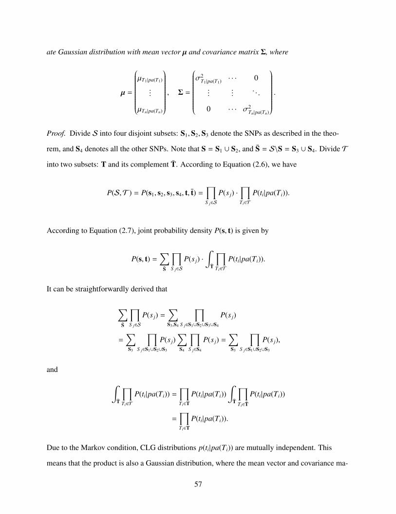
ate Gaussian distribution with mean vector µ and covariance matrix Σ, where

µ =

µT1 |pa(T1)

...

µTn |pa(Tn)

, Σ =

σ2

T1 |pa(T1) · · · 0...

.... . .

0 · · · σ2Tn |pa(Tn)

.

Proof. Divide S into four disjoint subsets: S1,S2,S3 denote the SNPs as described in the theo-

rem, and S4 denotes all the other SNPs. Note that S = S1 ∪ S2, and S = S\S = S3 ∪ S4. Divide T

into two subsets: T and its complement T. According to Equation (2.6), we have

P(S,T ) = P(s1, s2, s3, s4, t, t) =∏S j∈S

P(s j) ·∏Ti∈T

P(ti|pa(Ti)).

According to Equation (2.7), joint probability density P(s, t) is given by

P(s, t) =∑

S

∏S j∈S

P(s j) ·∫

T

∏Ti∈T

P(ti|pa(Ti)).

It can be straightforwardly derived that

∑S

∏S j∈S

P(s j) =∑S3,S4

∏S j∈S1∪S2∪S3∪S4

P(s j)

=∑S3

∏S j∈S1∪S2∪S3

P(s j)∑S4

∏S j∈S4

P(s j) =∑S3

∏S j∈S1∪S2∪S3

P(s j),

and ∫T

∏Ti∈T

P(ti|pa(Ti)) =∏Ti∈T

P(ti|pa(Ti))∫

T

∏Ti∈T

P(ti|pa(Ti))

=∏Ti∈T

P(ti|pa(Ti)).

Due to the Markov condition, CLG distributions p(ti|pa(Ti)) are mutually independent. This

means that the product is also a Gaussian distribution, where the mean vector and covariance ma-

57

trix can be directly obtained from the mean and variance of each CLG distribution. �

Based on Theorem 5, we provide the general inference formula as shown in Theorem 6.

Theorem 6. The probability for any desired value assignment to subsets Sx, Tx, given the ob-

served value assignment to disjoint subsets Sy, Ty, is given by

P(sx, tx|sy, ty) =P(sx, sy, tx, ty)

P(sy, ty),

where P(sx, sy, tx, ty) and P(sy, ty) are calculated according to Theorem 5.

There can be many applications of the inference. One typical application is to evaluate the health

risk, implied by a subset of traits, given the genotype profile and possibly a subset of other traits

of the user. This means to calculate posterior distribution P(tx|sy) or P(tx|ty, sy). For example, the

bone mineral density is known to be associated with several SNPs. Hence, we can predict the

bone mineral density in a certain period of lifetime based on the SNPs and some other traits such

as physical activities the target has. Another application can be to infer the genotype profile of a

user given an incomplete genotype record, i.e., to calculate P(sx|sy). By doing so, the user can in-

fer the genotype profile rather than doing another costly genotype scan. As another example, the

CLG Bayesian network can be used to infer the genotype profile of a target based on the traits the

target has, i.e., to calculate P(sx|ty). This inference can be used to evaluate the potential privacy

risk due to the statistics released in the GWAS catalog. We will evaluate the third application in

the experiments.

4.4. Further Extensions

So far, we make several assumptions in order to simplify the representation and ensure that the

CLG Bayesian network can be built from the GWAS catalog only. In this section, we briefly dis-

cuss the relaxation of the assumptions and the extensions of our model to these relaxed situations.

58

First, since the GWAS catalog does not include the correlations between SNPs, we assume no

edge among SNPs in the network. This assumption can be relaxed if additional knowledge is

available from other sources. For example, assume that we know the joint genotype frequency

of all correlated SNPs, and we also know the direction of the influence between each pair of cor-

related SNPs. Then we can easily incorporate the SNP-SNP correlations into our CLG Bayesian

network. For each correlated SNP pair, we simply add an edge between the two SNPs according

to the direction of the influence. The CPTs of SNPs can be specified based on the joint genotype

frequencies. On the other hand, if only SNP-SNP correlations without the direction exist, we can

merge the correlated SNPs as a single super node, representing and taking values from the com-

bination of the SNP genotypes. We add an edge pointing from the super node to each associated

traits. After that, similar to Theorems 5 and 6 all inferences can be conducted.

Second, we assume no edge among traits. The assumption may also be relaxed with additional

knowledge, where the network structure can be adapted based on trait-trait correlations. The only

limitation here is that, we don’t allow the edge to point from a quantitative trait to a categorical

trait, since the CLG Bayesian network assumes that discrete variables only have discrete parents.

As a result, we obtain a general CLG Bayesian network where each continuous variable can have

both discrete and continuous parents. In this case, the general belief propagation algorithms such

as [4, 29, 35] can be used for performing inference on the network.

4.5. Experiments

In this section, we first discuss our experimental setup and the CLG Bayesian network construc-

tion in Section 4.5.1. The inference methods are evaluated in Section 4.5.2. And finally, we con-

duct a case study to evaluate the individual information that can be inferred using the constructed

network.

59

4.5.1. CLG Bayesian Network Construction

We use data from the GWAS catalog of 5/24/2017. This version of the GWAS catalog includes

38,037 records (SNP-trait association pairs) extracted from 2,468 publications. Out these records,

there are a total of 28,943 SNPs associated with a total of 1,864 traits. For each record, the risk

allele type, the p-value, the sample description, and the odds ratio or β coefficient are provided.

Note that the odds ratio or the β coefficient is provided in the same field, depending on whether

the trait is categorical or quantitative.

In the experiments, we only consider the quantitative traits and focus on a subset of data used as

an interactive diagram (https://www.ebi.ac.uk/gwas/diagram) published by the GWAS catalog. In

this subset of data, an additional field “orType” is used to clearly indicate whether the odds ratio

is provided and hence indicate whether the trait is categorical or quantitative. This subset of data

includes 5,893 records which contains 809 traits and 4,643 SNPs. We extract the records with

“orType = false”, i.e., the trait is quantitative. As a result, we obtain 484 traits associated with

2,768 SNPs which are contained in 3,557 records. Finally, we build a knowledge database about

the traits and the associated SNPs, including the risk allele type, β coefficient, the p-value, and

the sample description for each trait-SNP association pair.

Table 4.1: Snapshot of CLG Bayesian network

Index Trait a0 c SNP-risk allele ai p(si)1 PCA3 expression level 15.599 26.661 rs10993994-T 1.250 {0.23, 0.50, 0.27}

2 Head circumference 47.307 0.535 rs7980687-A 0.074 {0.67, 0.30, 0.03}rs1042725-T -0.065 {0.17, 0.49, 0.34}

3 Fat body mass 24.621 0.576 rs6567160-C 0.090 {0.60, 0.35, 0.05}4 Iron levels 18.794 0.013 rs228916-T -0.086 {0.00, 0.14, 0.86}

5 Thyroid-stimulating hormone levels 2.047 0.684 rs12126655-G 0.138 {0.45, 0.44, 0.11}rs11026407-C -0.125 {0.31, 0.49, 0.20}

Based on the knowledge database, the CLG Bayesian network has been built according to Section

4.2. Table 4.1 shows the information and statistics of a snapshot of the network. There are 5 traits

and 7 associated SNPs in the snapshot, reported in 4 GWAS publications. For each trait, param-

eters a0 and c are shown in Columns 3 and 4. Column 5 shows each associated SNP of the trait,

60

along with the parameter ai and the genotype frequencies P(si) = {P(si =0), P(si =1), P(si =2)} as

shown in Columns 6 and 7.

4.5.2. Inference Evaluation

Figure 4.2: Posteriori probability densities of traits.

We evaluate the inference methods by considering two situations. In the first situation, we calcu-

late the CLG distribution of each trait given all SNPs, i.e., P(t|S) for each trait T , which is equiv-

alent to P(t|pa(T )). The results for the traits in Table 4.1 are shown in Figure 4.2, where each

subfigure corresponds to the trait with the same index in the table. In the subfigure, each dashed

line represents the CLG distribution given one value assignment to the associated SNPs. We also

plot the marginal distribution of the trait by marginalizing all CLG distributions, represented by

the solid line. It can be seen that, for traits such as PCA3 expression level and Iron level,

there are obvious differences in the marginal distribution and the CLG distributions, while for

traits such as Fat body mass, the difference is very small. The difference in the distributions

shows the difference in the strength of the influence of the associated SNPs on the trait.

In the second situation, we calculate the genotype frequencies of a subset of SNPs given the val-

ues of a subset of traits, i.e., P(s|t). We set the values of traits to three levels: in the first level, all

61

traits are set to their means; in the second level, all traits are set to their means plus their stan-

dard deviations; and in the third level, all traits are set to their means plus two times of their stan-

dard deviations. The results for the traits and SNPs in Table 4.1 are shown in Figure 4.3, where

each subfigure corresponds to one trait setting level. We can see that the distribution of each SNP

changes with the increase of the traits correspondingly to the sign of ai.

4.5.3. Application: Identity Inference

In this subsection, we consider an application where the CLG Bayesian network is used by an

attacker in identifying the identity information of a target individual from a genotype database.

Specifically, the attacker has access to an anonymized genotype database R which contains the

target’s genotype record sv. The attacker also knows a subset of traits tv the target has. Then, the

attacker can learn the posteriori probability of each genotype record si in the database given the

traits, i.e., P(si|tv), and use them to improve the identification success likelihood. Specifically,

the improved probability that the target’s record sv is identified is given by P(sv |tv)∑|R|i=1 P(si |tv)

. We evaluate

the performance of the attack by comparing the identification probability with that of the random

guess which uses no background knowledge.

We extract a genotype profile dataset from the 1000 Genomes Project [50] referred to as ‘CEU’,

which is used to serve as the anonymized genotype database. The ‘CEU’ dataset consists of 99

Figure 4.3: Posteriori probability distribution of SNPs.

62

HapMap individuals from Utah residents with Northern and Western European ancestry. For the

target, we manually generate his genotype and phenotype profiles at random. We assume that the

target has the minor traits, which means that the value of each trait is less than µ−σ or larger than

µ + σ. Thus, for each trait T , we randomly generate its value t according to the density P(t) with

the constraint t < µ − σ or t > µ + σ. After all traits t are generated, for each SNP S , we ran-

domly generate its value s according to the probability P(s|t). In this way, we simulate a scenario

where the target is randomly picked from the population with minor traits. After that, we blend

the genotype profile of the target into the ‘CEU’ dataset which contains the genotype records of

99 individuals, and attempt to re-identify it with the target’s traits just like what an attacker does.

We run this process 1,000 times, and evaluate the average probability of the target’s record to be

identified. We also compare the probability with different amount of knowledge, i.e., with the

size of trait set tv increasing from one to five.

Figure 4.4: Probability of identification.

The results are shown in Figure 4.4. The green dashed line is the baseline representing the iden-

tification probability 1/100 without any background knowledge. The red solid line represents the

average identification probability of our method along with the 15% and 85% percentiles. As can

be seen, the identification probability generally increases as the background knowledge increases.

The average identification probability of our method is larger than that of the random guess with-

63

out any background knowledge, implying the potential risk in privacy leak due to the statistics

released in GWAS catalog.

4.6. Related Work

Detecting and analyzing SNP-trait associations by building Bayesian networks has been studied

in biomedical fields. In [24] the authors used a score-based Bayesian network structure learn-

ing algorithm to detect epistasis or interactions among SNPs. In [12], the same problem was

addressed by using a new information-based score and a branch-and-bound search algorithm to

discover the structure of the Bayesian network. As an extension to the work of [24], in [60] the

authors proposed an exhaustive search on a Bayesian network to detect high order associations of

SNPs with traits, without requiring marginal effects on low dimensional datasets. All of the re-

lated work aforementioned requires a raw genotype-phenotype dataset to construct a Bayesian

network. However, the raw data required may not always be available. Different from above

works, in [56, 63], the authors studied the construction of Bayesian network from the released

GWAS statistics only. The two-layered Bayesian network was built and inference was conducted

using the constructed network. However, these works can only deal with the categorical traits.

Our work in this chapter uses the CLG Bayesian network to deal with the quantitative traits and is

readily to be extended to the mixture of categorical and quantitative traits.

Similar to the work in [63], we adopt the assumption of Independence of Causal Influence in

the specification of the CLG Bayesian network. The ICI is proposed to overcome the problem

of specifying a large number of conditional probability distributions for a dependent node with

multiple parents in the Bayesian network. Examples of widely used ICI models include Noisy-

Or, Sigmoid, Noisy-Max, and Noisy-Add [16]. The first three models target the situation where

the dependent node is a discrete variable, while the Noisy-Add model targets the situation where

the dependent node is a continuous variable. In our case, only the trait can be the dependent node

in the network. Thus, the Noisy-Add model is applied in this work.

64

4.7. Summary

In this chapter, we studied the exploration and modeling of associations between SNPs and quan-

titative traits from the GWAS catalog. The CLG Bayesian network which can deal with a mixture

of discrete and continuous variables is employed. We developed the method of constructing the

CLG Bayesian network only using the released statistics from the GWAS catalog, as well as in-

ference methods for calculating posterior distributions. We empirically evaluate the construction

and inference methods. The results show that important information can be inferred using the

constructed network. The work in this chapter is published in the Proceedings of the 2017 IEEE

International Conference on Bioinformatics and Biomedicine [61].

65

5. STIP: A SNP-Trait Inference Platform

5.1. Introduction

In the previous two chapters, we have proposed methods to build Bayesian networks using only

GWAS statistics instead of raw genotype data for characterizing SNP-trait associations and then

developed efficient formulas and algorithms to conduct SNP-trait inference based on the Bayesian

networks. In particular, we have proposed a three-layered traditional Bayesian network to model

the SNP-categorical trait associations in Chapter 3 and a two-layered Conditional Linear Gaus-

sian (CLG) Bayesian network to model the SNP-quantitative trait associations in Chapter 4.

In this chapter, we present STIP, a web-based platform that aims to aid common users in SNP-

trait inference and GWAS catalog exploration. STIP is based on Bayesian networks proposed

in Chapter 3 and 4 [61, 63]. Using STIP, users can easily infer SNPs/traits given their known

traits/SNPs and explore the SNP-trait associations. In particular, STIP provides three services:

1) SNP-trait inference allows users to conduct any kind of SNP-trait inference task, such as trait

inference given SNP genotypes or genotype inference given traits; 2) Top-k trait prediction shows

the probabilities of having some traits based on the user’s genotype profile; and 3) GWAS catalog

exploration helps users explore the SNP-trait associations.

Currently, there are some tools for GWA studies, like PLINK[44], GCTA[59]. However, only a

few systems have been developed to perform the SNP-trait inference. For example, hapassoc [2]

is an R package for likelihood inference of trait associations with SNP haplotypes. CGBayesNets[37]

is a MATLAB package that can build predictive models of a phenotype of interest using mul-

timodal genomic data as possible predictors. The existing packages require raw genotypes of

SNPs, yet such information is not publicly available. In this regard, all the data acquired by STIP

is from the GWAS catalog which can be accessed directly online. Without using sensitive geno-

type data, STIP can provide the SNP-trait inference service to public. Meanwhile, STIP can han-

dle both categorical and quantitative traits reported in the GWAS catalog, while previous plat-

66

forms only focus on one type of traits. Furthermore, unlike those packages that are designed for

genomic researchers, STIP has user friendly interface for general end users.

5.2. STIP Overview

STIP is a web-based platform for SNP-trait inference and GWAS catalog exploration. Figure 5.1

shows the architecture of STIP. Users can visit our platform through the URL: http://csce.

uark.edu/˜xintaowu/STIP.htm. Currently, STIP supports three services: (1) SNP-trait infer-

ence allows users to infer SNPs/traits by providing their known SNPs/traits. (2) Top-k trait pre-

diction helps users discover the risk of having a certain disease or identify significant changes of

quantitative traits based on their genotype profile. (3) GWAS catalog exploration allows users

to explore the SNP-trait associations especially when users find some unfamiliar SNPs or traits

from the previous two services. The back end of our platform is two Bayesian networks which

are derived from the GWAS catalog. All inference-related services are based on the constructed

Bayesian networks.

Figure 5.1: The architecture of STIP

5.2.1. Bayesian Network Construction

There are two types of traits in the GWAS catalog, categorical traits T c and quantitative traits T q.

For each type of trait, we construct a Bayesian network to model the relationships among traits

and SNPs.

67

The construction of the three-layered Bayesian network for modeling SNP-categorical traits

For categorical traits, a three-layered Bayesian network is constructed from the GWAS catalog,

which is designed to represent the conditional dependencies between categorical traits and SNPs.

The Bayesian network is consisted of three layers, the SNP genotype layer, the SNP allele layer,

and the categorical trait layer, from top to bottom. Please refer to Chapter 3 for detailed descrip-

tions.

To implement the Bayesian network, we adopt a subset of traits used as an interactive diagram

published by the GWAS catalog (https://www.ebi.ac.uk/gwas/diagram). In this subset of

data, an additional field “orType” is used to clearly indicate whether the odds ratio is provided. If

the value of “orType” is “True”, it indicates the trait is categorical. Otherwise, the trait is quanti-

tative.

After obtaining a categorical trait set T c, we then extract a set of SNPs S given those traits. For

each specific trait T ck ∈ T

c, we have a subset of associated SNPs Sk. For each associated SNP

S k j ∈ Sk, we can extract its corresponding risk allele type rk j associated trait T ck , the odds ratio

of the association test, and the risk allele frequency in the control group. If there exist multiple

entries for one SNP-trait pair, we only keep one SNP-trait association entry with the smallest p-

value. We further delete entries which do not contain risk allele, risk allele frequency in control

group, or odds ratio because those statistics are required in the three-layered Bayesian network

construction. To acquire the prior probability of each categorical trait, we classify all the cate-

gorical traits into 17 categories (e.g., immune system disease, nervous system disease, etc.), and

retrieve the average prevalence of each category from the Wikipedia. We use the average preva-

lence of a category as the prior probability of each trait belonging to the category. Our three-

layered Bayesian network can be refined by assigning the accurate prior probability for each trait

when available.

The three layer Bayesian network is constructed from the GWAS catalog. Because the GWAS

68

catalog extracts information from literature, one SNP-trait association may exist in the GWAS

catalog with multiple entries each of which may be submitted by one GWAS study and may have

different statistics values. For these duplicated entries, we only keep one SNP-trait association

entry with the smallest p-value. We further delete entries which do not contain risk allele, risk

allele frequency in control group, or odds ratio because those statistics are required in the three

layer Bayesian network construction.

Currently, STIP contains 265 categorical traits and their 2319 associated SNPs. Thus, the SNP

genotype layer, the SNP allele layer, and the trait layer in the three-layered Bayesian network

contain 2319, 2319, and 265 nodes, respectively. In particular, since each SNP has 2 alleles (e.g.,

A/G) and 3 genotypes (e.g., AA/AG/GG), each node in the SNP genotype layer has 3 values and

each node in the SNP allele layer has 2 values. STIP saves the statistics of each SNP-categorical

trait association in a JSON file. For each SNP-categorical trait association, the allele prior proba-

bilities, the genotype prior probabilities, the risk allele frequency of case and control groups and

the trait prior probability are included in the JSON file. The other conditional probabilities for

SNP-trait inference can be easily derived from the existing information when a user submits a

specific inference request. Figure 5.2a shows a code snippet about a SNP-categorical trait associ-

ation in the JSON file. In this example, the trait “Chronic kidney disease” is associated with one

SNP “rs6066043”. The allele and the genotype prior probabilities of that SNP are included in this

SNP-trait association. If a SNP is associated with multiple traits, those prior probabilities will be

included in all the related SNP-trait associations. This redundancy design improves the runtime

speed of the SNP-trait inference because the associated SNPs and their statistics can be directly

acquired by given a trait.

The construction of the CLG Bayesian network for modeling SNP-quantitative traits

We build a CLG Bayesian network for modeling SNP-quantitative trait associations. The CLG

Bayesian network contains two layers that are SNP genotype layer and quantitative trait layer. In

the CLG Bayesian network, the continuous variables (traits) only have discrete parents (SNPs).

69

Please refer to Chapter 4 for detailed descriptions.

Similar to the previous subsection, to implement the CLG Bayesian network, we obtain the fol-

lowing data from the GWAS catalog: a trait set T q and a SNP set S; for each trait T qk ∈ T

q, its

associated SNPs Sk; and for each SNP-trait pair, the coefficient β, p-value, and the sample size of

the specific study.

Currently, STIP contains 484 quantitative traits and their 2768 associated SNPs. Thus, the CLG

Bayesian network contains 484 nodes in the trait layer and 2768 nodes in the SNP genotype

layer. We use another JSON file to store the information of each SNP-quantitative trait associa-

tion. For each SNP-quantitative trait association, the genotype prior probabilities, trait distribu-

tion (µ and σ), and CLG distribution (coefficients and σ) are included in the JSON file. Figure

5.2b shows a code snippet about a SNP-quantitative trait association in the JSON file. In this ex-

ample, the trait “PCA3 expression level” is associated with one SNP “rs10993994”.

(a) SNP-categorical trait (b) SNP-quantitative trait

Figure 5.2: The information of SNP-trait associations stored in JSON files.

70

5.2.2. Services Provided by STIP

SNP-trait inference: The SNP-trait inference is the core service provided by STIP, which reports

the posterior probability of having any specific SNPs or traits given the already known SNPs or

traits. For example, we can calculate the posterior probability that a user has specific genotypes

for a set of SNPs given the user’s trait information.

In principle, we calculate the posterior probability for any desired assignment of values to vari-

able sets Sgx,Tx given the observed assignment of variable sets Sg

y ,Ty, as shown in Equation (5.1).

Note that Sgx and Sg

y denote the set of SNP genotypes; while Tx, Ty denote the set of traits.

P(sgx, tx|sg

y , ty) =P(sg

x, tx, sgy , ty)

P(sgy , ty)

. (5.1)

Equation (5.1) indicates that we can derive the posterior probability distribution of one or more

variables in the Bayesian network given the values observed for other variables in the network.

Meanwhile, Equation (5.1) shows that to conduct inference, we first need to calculate the joint

probability for any desired assignment of values to variable sets Sg of SNPs S and traits T, which

reflects the relationship among SNPs and traits.

For categorical traits, the joint probability for any value assignment to Sg of S ⊆ S, Tc ⊆ T c, i.e.,

P(sg, tc), based on the three-layered Bayesian network is defined as

P(sg, tc) =∏

S j∈S1

P(sgj)

∑Sa

2,Sg3,S

a3

( ∏S j∈S2∪S3

P(sgj)P(sa

j |sgj)

∏T c

k∈Tc

P(tck|pa(T c

k ))), (5.2)

where S1 denotes the SNPs in S but not associated with Tc, S2 denotes the SNPs in S and also

associated with Tc, S3 denotes the SNPs associated with Tc but not in S.

For quantitative traits, the joint probability density for any value assignment to subsets Sg of S ⊆

71

S, Tq ⊆ T q is given by

P(sg, tq) =∑S3

∏S g

j∈S1∪S2∪S3

P(sgj) · N(tq;µ,Σ), (5.3)

where S1 denotes the SNPs in S but not associated with Tq; S2 denotes the SNPs in S and are also

associated with Tq; S3 denotes the SNPs associated with Tq but not in S; N(t;µ,Σ) is a multivari-

ate Gaussian distribution with mean vector µ and covariance matrix Σ, where

µ =

µtq1 |pa(T q

1 )

...

µtqn |pa(T qn )

, Σ =

σ2

tq1 |pa(T q1 )· · · 0

......

. . .

0 · · · σ2tqn |pa(T q

n )

.

All terms in Equations (5.2) and (5.3) are completely specified in the two Bayesian networks.

Top-k trait prediction: The top-k trait prediction is a special case of SNP-trait inference, i.e.,

trait inference given SNP genotypes.

For categorical traits, this service lists the top-k traits of a user that have the most significant in-

crease from the trait prior probabilities to the trait posterior probabilities by inferring from the

user’s genotype profile. Formally we represent the genotypes of a user as sg = (sg1, s

g2, · · · , s

gn),

with each entry sgj indicating the genotype of SNP j. The trait inference given SNP genotypes

aims to learn the posterior probability P(tc = 1|sg) that a user has a specific trait tc given the tar-

get’s genotype profile sg using the Bayesian network. The posterior probability P(tc = 1|sg) can

be calculated based on Equation (5.1) with sgx = ∅, tc

y = ∅, tcx = {t}, and sg

y = sg. After calcu-

lating the posterior probability P(tc = 1|sg), we further compute the change value for each trait

Ltc = P(tc = 1|sg) − P(tc = 1) and show traits with the top-k largest Ltc .

For quantitative traits, this service lists the top-k traits of a user that have the most significant

change from the mean value of the trait E(tq) to the mean value of the trait given the user’s geno-

type profile E(tq|sg) based on the CLG Bayesian network. The mean value of the trait can be ac-

72

quired from the Internet or literature. The posterior mean value of the trait is defined as

E[tq|sg] = a0 +

m∑i=1

aisi, (5.4)

where ai (i = 0; · · · ; m) are the CLG distribution coefficients of the associated SNPs given

the trait tq. After calculating E(tq|sg), we further compute the change value for each trait Ltq =

|E(tq|sg) − E(tq)| and show traits with the top-k largest Ltq .

Figure 5.3 shows the procedures of using SNP-trait inference and Top-k trait prediction services.

For SNP-trait inference, the known SNPs/traits are first specified and then STIP will report the

probabilities of unknown SNPs/traits based on the Bayesian network. For Top-k trait predic-

tion, users first submit their genetic file. STIP will report the probabilities or mean values of traits

given the genotype profile.

GWAS catalog exploration: The third service provided by STIP is the GWAS catalog explo-

ration. Although the GWAS catalog website allows users to search SNPs and traits, the search

results are organized by the studies and do not clearly show the SNP-trait associations. Unlike the

exploration provided by the GWAS catalog website, STIP provides trait-SNP and SNP-trait asso-

ciation explorations which allow users to choose a trait (SNP) and then show the associated SNPs

(traits).

Figure 5.3: The procedures of SNP-trait inference and Top-k trait prediction

73

5.3. Demonstration

Since STIP is a web-based platform, users can visit STIP through an Internet browser. In this

section, we illustrate the use of the three services provided by STIP.

Figure 5.4: SNP-categorical trait inference web UI with an example of trait inference given SNPgenotypes and categorical traits

5.3.1. SNP-Trait Inference

Users can perform SNP-trait inferences on the “SNP-Categorical Trait Inference” and “SNP-

Quantitative Trait Inference” pages. Users can first choose the known traits from the trait list and

the known SNPs from the SNP list. Due to the large number of SNPs and traits, STIP provides

search bars for both lists which allow users to search a specific SNP and trait. Users can choose

multiple traits or SNPs at a time. Once users have selected the known traits and SNPs, they can

further click the “Known Traits” and “Known SNPs” buttons. The selected traits and SNPs will

be added to the “Known Traits (Ty)” and “Known SNPs (S y)” lists on the right side of the page.

In particular, for a categorical trait T cy ∈ {Y,N}, Y indicates a user with the trait and N indicates

74

the user without the trait. For a quantitative trait, the default value of T qy ∈ (−∞,∞), users can

specify the range of the T qy based on their knowledge. Users can also specify the genotypes of

each SNP. Then, users can further select the inference traits and SNPs by clicking the “Inference

Traits” and “Inference SNPs”. Finally, users can click the “Inference” button to get the result of

the specified inference. Figure 5.4 shows an example of SNP-categorical trait inference. In this

example, STIP reports the probability of a user with the trait “Psoriasis” by knowing that the user

has two traits and three SNPs. The “SNP-Quantitative Trait Inference” has a similar UI which al-

lows user to specify the range of a quantitative trait. Note that both pages provides general SNP-

trait inference services which allow users to do any kind of inference without the need to specify

all the lists on the right side of the pages. For example, if a user only knows some of the traits and

wants to know the risk of having other traits, the user can just specify the “Known Traits (Ty)”

and “Inference Traits (Tx)” and then runs the inference.

(a) Top-10 trait prediction (b) General trait prediction

Figure 5.5: Top-k trait prediction web UIs with results of trait prediction given a user’s geneticfile

5.3.2. Top-K Trait Prediction

The “Top-K Trait Prediction” allows a user to submit his/her genetic file and reports the probabil-

ities (mean values) of traits based on the genotype profile. Currently, STIP supports the genetic

file provided by 23andme (https://www.23andme.com/). Figure 5.5 shows the result page af-

ter a user submits the genetic file. There are three tabs in the “Top-K Trait Prediction” page. The

75

first one is the “Top-K Categorical Traits” tab (shown in Figure 5.5a) which shows top-k categor-

ical traits with the largest increase values from trait prior probabilities to posterior probabilities

given SNPs. The second one is the “Top-K Quantitative Traits” tab which shows top-k quantita-

tive traits with the largest change values from trait prior mean values to posterior mean values.

The last one is “All Traits” tab (shown in Figure 5.5b) which lists all the traits associated with the

user’s genotypes. For each categorical (quantitative) trait, STIP reports the trait prior and poste-

rior probabilities (mean values), the change value between the trait prior and posterior probabili-

ties (mean values), the associated SNPs, and the genotypes of the user.

(a) Exploring SNP-Trait associations (b) Exploring Trait-SNP associations

Figure 5.6: GWAS catalog exploration web UIs

5.3.3. GWAS Catalog Exploration

STIP provides two separated pages for SNP-trait and trait-SNP association explorations. Figure

5.6a shows the SNP-trait association exploration where a user can explore the associated traits by

providing a specific SNP. In this scenario, once a user chooses a SNP, the SNP-trait association

page shows the number of associated traits and lists all the information about those traits. Figure

5.6b shows the trait-SNP association exploration where a user can explore the associated SNPs

by specifying a trait.

76

5.4. Summary

We present STIP, a web-based platform that provides the SNP-trait inference and GWAS-catalog

exploration. The SNP-trait inference is designed to infer the probabilities of unknown traits/SNPs

by given known traits/SNPs. STIP also allows users to submit their genetic file and reports the

risks of having specific traits based on their genotype profile. The GWAS-catalog exploration

is designed to explore the SNP-trait associations. The work in this chapter is published in the

Proceedings of the 2017 IEEE International Conference on Bioinformatics and Biomedicine [42].

77

6. Conclusions and Future Work

6.1. Conclusions

In this thesis, we studied the construction of the Bayesian networks from the public released

GWAS catalog for modeling SNP and trait associations. Bayesian network has been proposed

as a powerful tool for modeling SNP-trait associations. Most of existing works learn the Bayesian

network from the raw data. However, due to privacy issue, genotype information is classified as

sensitive which should be dealt with by complying with specific restrictions. To tackle this limi-

tation, we proposed to build Bayesian networks from the GWAS catalog. The GWAS catalog is a

database that collects and publicly releases literature-derived GWAS statistics, including pairwise

SNP-trait associations, risk allele frequency, p-value, etc. In particular, since there are two types

of traits (i.e., categorical trait and quantitative trait), we develop two types of Bayesian networks

correspondingly to model the SNP-trait associations from the GWAS statistics.

First, we developed a method of building a classic three-layered Bayesian network using only

GWAS statistics for characterizing SNP-categorical trait associations. In order to construct a

Bayesian network from only statistics, we derived a formulation based on the Noisy-Or model,

one best known example of the independence of causal influence (ICI) models, that can be used

to specify the conditional probability table (CPT) from the released GWAS statistics where the

underlying genotypes can be unknown. We theoretically and empirically validated the fitness of

using the Noisy-Or model to specify CPT. Based on the constructed Bayesian network, we fur-

ther conducted inference tasks including trait inference given SNP genotype, genotype inference

given trait, and trait inference given trait. We showed that significant amount of knowledge re-

garding traits can be inferred from the genotype profiles and the probability of an individual to be

identified from an anonymized genotype database was increasing given some traits of the individ-

ual.

Second, we employed a CLG Bayesian network which can deal with a mixture of discrete and

78

continuous variables to model SNP-quantitative trait associations from GWAS statistics. Sepcif-

ically, SNPs are represented as discrete variables, and the quantitative traits are represented as

continuous variables. We then developed the inference methods to conduct SNP-quantitative trait

inference tasks. The empirical results showed the effectiveness of our methods.

Finally, we developed STIP, a web-based platform that provided the SNP-trait inference and

GWAS-catalog exploration. The SNP trait inference was designed to infer the probabilities of un-

known traits/SNPs by given known traits/SNPs. STIP also allowed users to submit their genetic

file and reported the risks of having specific traits based on their genotype profile.

6.2. Future Work

Our work can be further improved in the following directions:

Firstly, for simplicity we assume all traits are quantitative in the CLG Bayesian network. Since

the CLG Bayesian network is able to deal with both continuous and categorical data, our model is

readily to handle the mixture of categorical and quantitative traits. In the future, we plan to model

the both categorical and quantitative traits in one unified CLG Bayesian network. In this case, be-

sides the genotype frequencies and CLG distributions for quantitative traits, we also need to spec-

ify the CPTs for the categorical traits. This can be done by directly adopting the method proposed

in [63]. After the network construction completes, all inferences can be performed similarly as

shown in Theorems 5 and 6.

Second, we also plan to integrate the SNP-SNP correlations and trait-trait correlations into our

model if additional knowledge is available from other sources.

Finally, we plan to develop methods to enable researchers to safely release aggregate GWAS data

without compromising the anonymity of both GWAS participants and the general population.

79

Bibliography

[1] Bhaskar, R., Laxman, S., Smith, A., and Thakurta, A. Discovering frequent patternsin sensitive data. In Proceedings of the 16th ACM SIGKDD international conference onKnowledge discovery and data mining (2010), ACM, pp. 503–512.

[2] Burkett, K., Graham, J., McNeney, B., et al. hapassoc: Software for likelihood inferenceof trait associations with snp haplotypes and other attributes. Journal of Statistical Software16, 2 (2006), 1–19.

[3] Bush, W. S., Moore, J. H., Li, J., McDonnell, S., and Rabe, K. Chapter 11: Genome-WideAssociation Studies. PLoS Computational Biology 8, 12 (dec 2012), e1002822.

[4] Cowell, R. G. Local propagation in conditional gaussian bayesian networks. Journal ofMachine Learning Research 6, Sep (2005), 1517–1550.

[5] Dwork, C., McSherry, F., Nissim, K., and Smith, A. Calibrating noise to sensitivity in pri-vate data analysis. Theory of Cryptography (2006), 265–284.

[6] Edwards, A. W. Foundations of mathematical genetics. Cambridge University Press, 2000.

[7] Erlich, Y., and Narayanan, A. Routes for breaching and protecting genetic privacy. NatureReviews Genetics 15, 6 (2014), 409–421.

[8] Fienberg, S. E., Slavkovic, A., and Uhler, C. Privacy preserving gwas data sharing. In DataMining Workshops (ICDMW), 2011 IEEE 11th International Conference on (2011), IEEE,pp. 628–635.

[9] Friedman, N., Geiger, D., and Goldszmidt, M. Bayesian network classifiers. Machinelearning 29, 2-3 (1997), 131–163.

[10] Greshake, B., Bayer, P. E., Rausch, H., and Reda, J. Opensnp–a crowdsourced web re-source for personal genomics. PLoS One 9, 3 (2014), e89204.

[11] Gymrek, M., McGuire, A. L., Golan, D., Halperin, E., and Erlich, Y. Identifying personalgenomes by surname inference. Science 339, 6117 (2013), 321–324.

[12] Han, B., Chen, X.-w., Talebizadeh, Z., and Xu, H. Genetic studies of complex human dis-eases: Characterizing snp-disease associations using bayesian networks. BMC systems biol-ogy 6, Suppl 3 (2012).

[13] Heckerman, D. Causal independence for knowledge acquisition and inference. In Proceed-ings of the Ninth international conference on Uncertainty in artificial intelligence (1993),Morgan Kaufmann Publishers Inc., pp. 122–127.

[14] Heckerman, D. A Tutorial on Learning with Bayesian Networks. In Innovations inBayesian Networks. Springer Berlin Heidelberg, Berlin, Heidelberg, 2008, pp. 33–82.

80

[15] Heckerman, D., and Breese, J. S. A new look at causal independence. In UAI’94 (1994),Morgan Kaufmann Publishers Inc., pp. 286–292.

[16] Heckerman, D., and Breese, J. S. Causal independence for probability assessment and in-ference using bayesian networks. IEEE Trans. Syst., Man, Cybern. A, Syst.,Humans 26, 6(1996), 826–831.

[17] Hindorff, L., MacArthur, J., Morales, J., Junkins, H., Hall, P., Klemm, A., and Manolio,T. A catalog of published genome-wide association studies.

[18] Homer, N., Szelinger, S., Redman, M., Duggan, D., Tembe, W., Muehling, J., Pearson,J. V., Stephan, D. A., Nelson, S. F., and Craig, D. W. Resolving individuals contributingtrace amounts of dna to highly complex mixtures using high-density snp genotyping mi-croarrays. PLoS Genet 4, 8 (2008), e1000167.

[19] Humbert, M., Ayday, E., Hubaux, J.-P., and Telenti, A. Quantifying interdependent risks ingenomic privacy. ACM Transactions on Privacy and Security (TOPS) 20, 1 (2017), 3.

[20] Humbert, M., Huguenin, K., Hugonot, J., Ayday, E., and Hubaux, J.-P. De-anonymizing ge-nomic databases using phenotypic traits. Proceedings on Privacy Enhancing Technologies2015, 2 (2015), 99–114.

[21] Jacobs, K. B., Yeager, M., Wacholder, S., Craig, D., Kraft, P., Hunter, D. J., Paschal, J.,Manolio, T. A., Tucker, M., Hoover, R. N., et al. A new statistic and its power to infermembership in a genome-wide association study using genotype frequencies. Nature genet-ics 41, 11 (2009), 1253–1257.

[22] Jensen, F. V. An introduction to Bayesian networks, vol. 210. UCL press London, 1996.

[23] Jensen, F. V., and Nielsen, T. D. Bayesian Networks and Decision Graphs. InformationScience and Statistics. Springer New York, New York, NY, 2007.

[24] Jiang, X., Neapolitan, R. E., Barmada, M. M., and Visweswaran, S. Learning genetic epis-tasis using bayesian network scoring criteria. BMC bioinformatics 12, 1 (2011), 1.

[25] Johnson, A., and Shmatikov, V. Privacy-preserving data exploration in genome-wide as-sociation studies. In Proceedings of the 19th ACM SIGKDD international conference onKnowledge discovery and data mining (2013), ACM, pp. 1079–1087.

[26] Kim, J. H., and Pearl, J. A computational model for causal and diagnostic reasoning ininference systems. In IJCAI (1983), vol. 83, pp. 190–193.

[27] Kjærulff, U. B., and Madsen, A. L. Probabilistic networks: an introduction to bayesiannetworks and influence diagrams.

[28] Kosinski, M., Stillwell, D., and Graepel, T. Private traits and attributes are predictablefrom digital records of human behavior. Proceedings of the National Academy of Sciences

81

110, 15 (2013), 5802–5805.

[29] Lauritzen, S. L., and Jensen, F. Stable local computation with conditional gaussian distribu-tions. Statistics and Computing 11, 2 (2001), 191–203.

[30] Li, N., Qardaji, W., and Su, D. On sampling, anonymization, and differential privacy or,k-anonymization meets differential privacy. In Proceedings of the 7th ACM Symposium onInformation, Computer and Communications Security (2012), ACM, pp. 32–33.

[31] Lin, Z., Owen, A., and Altman, R. Genomic research and human subject privacy. Science305, 5681 (2004).

[32] Loeliger, H.-A. An introduction to factor graphs. IEEE Signal Processing Magazine 21, 1(2004), 28–41.

[33] MacArthur, J., et al. The new nhgri-ebi catalog of published genome-wide associationstudies (gwas catalog). Nucleic Acids Research 45, D1 (2017), D896–D901.

[34] MacCallum, R. C., Browne, M. W., and Sugawara, H. M. Power analysis and determina-tion of sample size for covariance structure modeling. Psychological methods 1, 2 (1996),130.

[35] Madsen, A. L. Belief update in clg bayesian networks with lazy propagation. InternationalJournal of Approximate Reasoning 49, 2 (2008), 503–521.

[36] Masca, N., Burton, P. R., and Sheehan, N. A. Participant identification in genetic associ-ation studies: improved methods and practical implications. International journal of epi-demiology 40, 6 (2011), 1629–1642.

[37] McGeachie, M. J., Chang, H.-H., and Weiss, S. T. Cgbayesnets: conditional gaussianbayesian network learning and inference with mixed discrete and continuous data. PLoScomputational biology 10, 6 (2014), e1003676.

[38] McLachlan, G., and Krishnan, T. The EM algorithm and extensions, vol. 382. John Wiley& Sons, 2007.

[39] Naveed, M., Ayday, E., Clayton, E. W., Fellay, J., Gunter, C. A., Hubaux, J.-P., Malin,B. A., and Wang, X. Privacy in the genomic era. ACM Computing Surveys (CSUR) 48, 1(2015), 6.

[40] Neal, R. M. Connectionist learning of belief networks. Artificial intelligence 56, 1 (1992),71–113.

[41] Nielsen, T. D., and Jensen, F. V. Bayesian networks and decision graphs. Springer Science& Business Media, 2009.

[42] Pan, Q., , Zhang, L., and Wu, X. Stip: A snp-trait inference platform. In Bioinformatics and

82

Biomedicine (BIBM), 2017 IEEE International Conference on (2017), IEEE.

[43] Pearl, J. Causality. Cambridge university press, 2009.

[44] Purcell, S., Neale, B., Todd-Brown, K., Thomas, L., Ferreira, M. A., Bender, D., Maller,J., Sklar, P., De Bakker, P. I., Daly, M. J., et al. Plink: a tool set for whole-genome associ-ation and population-based linkage analyses. The American Journal of Human Genetics 81,3 (2007), 559–575.

[45] Raisaro, J. L., Tramer, F., Ji, Z., Bu, D., Zhao, Y., Carey, K., Lloyd, D., Sofia, H., Baker,D., Flicek, P., et al. Addressing beacon re-identification attacks: Quantification and mitiga-tion of privacy risks. Tech. rep., 2016.

[46] Samani, S. S., Huang, Z., Ayday, E., Elliot, M., Fellay, J., Hubaux, J.-P., and Kutalik, Z.Quantifying genomic privacy via inference attack with high-order snv correlations. In Secu-rity and Privacy Workshops (SPW), 2015 IEEE (2015), IEEE, pp. 32–40.

[47] Sankararaman, S., Obozinski, G., Jordan, M. I., and Halperin, E. Genomic privacy andlimits of individual detection in a pool. Nature genetics 41, 9 (2009), 965–967.

[48] Shi, X., and Wu, X. An overview of human genetic privacy. Annals of the New YorkAcademy of Sciences (2016).

[49] Shringarpure, S. S., and Bustamante, C. D. Privacy risks from genomic data-sharing bea-cons. The American Journal of Human Genetics 97, 5 (2015), 631–646.

[50] The 1000 Genomes Project Consortium. An integrated map of genetic variation from 1,092human genomes. Nature 491 (2012), 1.

[51] Tramer, F., Huang, Z., Hubaux, J.-P., and Ayday, E. Differential privacy with bounded pri-ors: reconciling utility and privacy in genome-wide association studies. In Proceedingsof the 22nd ACM SIGSAC Conference on Computer and Communications Security (2015),ACM, pp. 1286–1297.

[52] Turner, S., et al. Quality control procedures for genome-wide association studies. Currentprotocols in human genetics (2011), 1–19.

[53] Visscher, P. M., and Hill, W. G. The limits of individual identification from sample allelefrequencies: theory and statistical analysis. PLoS genetics 5, 10 (2009), e1000628.

[54] Vomlel, J. Noisy-or classifier. International Journal of Intelligent Systems 21, 3 (2006),381–398.

[55] Wang, R., Li, Y. F., Wang, X., Tang, H., and Zhou, X. Learning your identity and diseasefrom research papers: information leaks in genome wide association study. In Proceed-ings of the 16th ACM conference on Computer and communications security (2009), ACM,pp. 534–544.

83

[56] Wang, Y., Wu, X., and Shi, X. Using aggregate human genome data for individual iden-tification. In Proceedings of the IEEE International Conference on Bioinformatics andBiomedicine. 2013, pp. 410–415.

[57] Welter, D., et al. The nhgri gwas catalog, a curated resource of snp-trait associations.Nucleic acids research 42, D1 (2014), D1001–D1006.

[58] Wikipedia. Copd.http://en.wikipedia.org/wiki/copd.

[59] Yang, J., Lee, S. H., Goddard, M. E., and Visscher, P. M. Gcta: a tool for genome-widecomplex trait analysis. The American Journal of Human Genetics 88, 1 (2011), 76–82.

[60] Zeng, Z., Jiang, X., and Neapolitan, R. Discovering causal interactions using bayesian net-work scoring and information gain. BMC bioinformatics 17, 1 (2016), 1.

[61] Zhang, L., Pan, Q., , and Wu, X. Modeling snp and quantitative trait association from gwascatalog using clg bayesian network. In Bioinformatics and Biomedicine (BIBM), 2017 IEEEInternational Conference on (2017), IEEE.

[62] Zhang, L., Pan, Q., Wang, Y., Wu, X., and Shi, X. Bayesian network construction andgenotype-phenotype inference using gwas statistics. IEEE/ACM Transactions on Compu-tational Biology and Bioinformatics PP, 99 (2017), 1–1.

[63] Zhang, L., Pan, Q., Wu, X., and Shi, X. Building bayesian networks from gwas statisticsbased on independence of causal influence. In Bioinformatics and Biomedicine (BIBM),2016 IEEE International Conference on (2016), IEEE, pp. 529–532.

[64] Zhou, X., Peng, B., Li, Y. F., Chen, Y., Tang, H., and Wang, X. To release or not to release:evaluating information leaks in aggregate human-genome data. In Computer Security–ESORICS 2011. Springer, New York, 2011, pp. 607–627.

84