fnins-12-00598 September 26, 2018 Time: 18:13 # 1

METHODSpublished: 28 September 2018doi: 10.3389/fnins.2018.00598

Edited by:Srikantan S. Nagarajan,University of California,

San Francisco, United States

Reviewed by:Gareth Barnes,

University College London,United Kingdom

Karl Friston,University College London,

United Kingdom

*Correspondence:Clare D. Harris

clare.harris@uqconnect.edu.au

†Shared first authorship

Specialty section:This article was submitted to

Brain Imaging Methods,a section of the journal

Frontiers in Neuroscience

Received: 01 February 2018Accepted: 08 August 2018

Published: 28 September 2018

Citation:Harris CD, Rowe EG, Randeniya R

and Garrido MI (2018) BayesianModel Selection Maps for Group

Studies Using M/EEG Data.Front. Neurosci. 12:598.

doi: 10.3389/fnins.2018.00598

Bayesian Model Selection Maps forGroup Studies Using M/EEG DataClare D. Harris1*†, Elise G. Rowe2†, Roshini Randeniya1 and Marta I. Garrido1,3,4,5

1 Computational Cognitive Neuroscience Laboratory, Queensland Brain Institute, The University of Queensland, Brisbane,QLD, Australia, 2 Monash Neuroscience of Consciousness Laboratory, School of Psychological Sciences, Faculty ofMedicine Nursing and Health Science, Monash University, Melbourne, VIC, Australia, 3 School of Mathematics and Physics,The University of Queensland, Brisbane, QLD, Australia, 4 Australian Research Council Centre of Excellence for IntegrativeBrain Function, Monash University, Melbourne, VIC, Australia, 5 Centre for Advanced Imaging, The University of Queensland,Brisbane, QLD, Australia

Predictive coding postulates that we make (top-down) predictions about the worldand that we continuously compare incoming (bottom-up) sensory information withthese predictions, in order to update our models and perception so as to betterreflect reality. That is, our so-called “Bayesian brains” continuously create and updategenerative models of the world, inferring (hidden) causes from (sensory) consequences.Neuroimaging datasets enable the detailed investigation of such modeling and updatingprocesses, and these datasets can themselves be analyzed with Bayesian approaches.These offer methodological advantages over classical statistics. Specifically, any numberof models can be compared, the models need not be nested, and the “null model” canbe accepted (rather than only failing to be rejected as in frequentist inference). Thismethodological paper explains how to construct posterior probability maps (PPMs) forBayesian Model Selection (BMS) at the group level using electroencephalography (EEG)or magnetoencephalography (MEG) data. The method has only recently been usedfor EEG data, after originally being developed and applied in the context of functionalmagnetic resonance imaging (fMRI) analysis. Here, we describe how this method canbe adapted for EEG using the Statistical Parametric Mapping (SPM) software packagefor MATLAB. The method enables the comparison of an arbitrary number of hypotheses(or explanations for observed responses), at each and every voxel in the brain (sourcelevel) and/or in the scalp-time volume (scalp level), both within participants and at thegroup level. The method is illustrated here using mismatch negativity (MMN) data froma group of participants performing an audio-spatial oddball attention task. All data andcode are provided in keeping with the Open Science movement. In doing so, we hopeto enable others in the field of M/EEG to implement our methods so as to address theirown questions of interest.

Keywords: EEG, MEG, Bayes, PPMs, BMS, code:matlab, code:spm

INTRODUCTION

The statistical testing of hypotheses originated with Thomas Bayes (Neyman and Pearson, 1933),whose famous eponymous theorem (Bayes and Price, 1763) can be written in terms of probabilitydensities as follows:

p(θ|y)

=p(y∣∣θ)p(θ)p(y)

(1)

Frontiers in Neuroscience | www.frontiersin.org 1 September 2018 | Volume 12 | Article 598

fnins-12-00598 September 26, 2018 Time: 18:13 # 2

Harris et al. BMS Maps Using M/EEG Data

where θ denotes unobserved parameters, y denotes observedquantities, and p(θ|y) denotes the probability p of the unknownparameters θ, given (“|”) the set of observed quantities y. Moregenerally, p(event|knowledge) denotes the probability of an eventgiven existing knowledge. In other words, Bayes conceptualizesstatistics as simply the plausibility of a hypothesis given theknowledge available (Meinert, 2012).

Bayes’ theorem allows one to update one’s knowledge ofthe previously estimated (or “prior”) probability of causes, toa new estimate, the “posterior” probability of possible causes.This process can be repeated indefinitely, with the prior beingrecursively updated to the new posterior each time. This givesrise to multiple intuitive and useful data analysis methods, oneof which is the explained in detail in this paper.

Even when it first appeared, Bayes’ theorem was recognizedas an expression of “common sense,” a “foundation for allreasonings concerning past facts,” (Bayes and Price, 1763).Centuries later, neuroscientific evidence suggests that Bayes’theorem may not only explain our “common sense” and internalreasoning processes, but may be common to all our senses: itcan actually explain the way in which we use our various sensesto perceive the world. That is, Bayesian statistics can be used toaccurately model and predict the ways in which our own brainsprocess information (Dayan et al., 1995; Feldman and Friston,2010; Friston, 2012; Hohwy, 2013). This has given rise to theconcepts of predictive coding and the Bayesian brain. In thiscontext, it is unsurprising that Bayesian approaches to statisticshave high face validity (Friston and Penny, 2003). This allowsfor intuitive descriptions of probability and enables experimentalresults to be relatively easily understood and communicated bothwithin and between scientific communities, as well as to thegeneral public (Dunson, 2001).

Despite the intuitiveness of Bayesian approaches, however, themainstay of hypothesis-testing since the 20th century (Vallverdú,2008) has instead been classical or frequentist statistics, whichconceptualizes probability as a “long-run frequency” of events,and which has dominated most approaches to neuroimaginganalysis to date (Penny et al., 2003). For example, creatingstatistical parametric maps (SPMs), which is a popular methodof analyzing neuroimaging data, mainly involves frequentistapproaches (Friston and Penny, 2003).

In frequentist statistics, the null hypothesis (that there is norelationship between the causes and the data) is compared withone alternative hypothesis; the null is then either rejected infavor of the alternative hypothesis, or it fails to be rejected – itcan never be directly “supported.” Rejection of the null dependson the somewhat unintuitive p-value, which communicates howlikely it is that the effect (of at least the size seen in theexperiment), would be seen in the absence of a true effect, if theexperiment were repeated many times. This is a more complexand counterintuitive way of communicating results compared toBayesian statistics (where the probability of the hypothesis inquestion is what is being estimated and communicated).

Also, unfortunately, multiple different models cannot becompared at once, and either the null and the alternative modelsneed to be nested, or specific modifications need to be made(Horn, 1987; McAleer, 1995), for frequentist statistical tests to

be feasible (Rosa et al., 2010). These features cause frequentiststatistics to be less useful in certain contexts, compared to theapproaches enabled by Bayesian statistics.

In recent decades, Bayesian approaches are becomingincreasingly recognized for their superior utility for addressingcertain questions and in specific data analysis situations, asexplained below (Beal, 2003; Rosa et al., 2010; Penny andRidgway, 2013). Importantly, with Bayesian approaches to dataanalysis, any number of models can be compared, the modelsneed not be nested, and the “null model” can be accepted (Rosaet al., 2010). The fact that Bayesian hypothesis-testing also allowsresearchers to evaluate the likelihood of the null hypothesis iscrucially important in light of the replication crisis in psychologyand neuroscience (Hartshorne, 2012; Larson and Carbine, 2017;Szucs et al., 2017). Importantly, results supporting the nullhypothesis are equally noteworthy or reportable as other resultswithin Bayesian statistics. The use of Bayesian statistics may alsoameliorate some statistical power-related problems documentedin the literature (Dienes, 2016).

Even though Bayesian statistics has gained popularity inthe context of “accepting the null,” its strength lies beyondthis, in the sense that it enables the relative quantification ofany number of alternative models (or hypotheses). In BayesianModel Selection (BMS), models are compared based on theprobability of observing a particular dataset given each model’sparameters. The probability of obtaining observed data, y, givenmodel m, p(y|m), is known as the model evidence. In BMS, anapproximation of the model evidence is calculated for multiplemodels; the model evidences are then compared to determinewhich model returns the highest probability of generating theparticular dataset in question (Rosa et al., 2010).

A computationally efficient and relatively accurate (Stephanet al., 2009) method of approximating the model evidence is touse variational Bayes (VB). If each participant in the dataset isassumed to have the same model explaining their data, then this iscalled a fixed effects (FFX) approach. If, on the other hand, everyparticipant is permitted to have their own (potentially different)model, this is called a random effects (RFX) approach.

An elegant approach to succinctly communicating resultsis to use Posterior Probability Maps (PPMs), which providea visual depiction of the spatial and/or temporal locations inwhich a particular model is more probable than the alternativesconsidered, given the experimental data in question. Thedevelopment of PPMs is essentially the Bayesian alternative to thecreation of SPMs (Friston and Penny, 2003). PPMs may displaythe posterior probability of the models (the probability that amodel explains the data), or, alternatively, they may be displayedas Exceedance Probability Maps (EPMs), which are maps of theprobabilities that a model (say k) is more likely compared to allother (K) models considered (Rosa et al., 2010). (EPMs will beidentical to PPMs in cases where there are only two models beingconsidered, as in this study.) EPMs are useful in that they allowus to directly quantify which model is more probable than theother/s considered.

The data analysis method that forms the focus of this paperis Posterior Probability Mapping with an RFX approach to VB.First introduced (Rosa et al., 2010) for functional magnetic

Frontiers in Neuroscience | www.frontiersin.org 2 September 2018 | Volume 12 | Article 598

fnins-12-00598 September 26, 2018 Time: 18:13 # 3

Harris et al. BMS Maps Using M/EEG Data

resonance imaging (fMRI), the method has recently been adaptedfor inference using electroencephalography (EEG) data (Garridoet al., 2018). In their study, Garrido et al. (2018) used VB toapproximate the log of the model evidence for each voxel (inspace and time) in every participant, in order to construct PPMsat the group level. They did this in the context of comparingbetween two computational models describing the relationshipbetween attention and prediction in auditory processing. Whilethat paper focused on using this Bayesian methodology to addressan important neuroscientific question, the precise way in whichRosa and colleagues’ (2010) methods were adapted for use withEEG data, has not been formally described to date – leading tothe purpose of this paper.

Here, we describe in a tutorial-like manner how to buildand compare PPMs for EEG and/or magnetoencephalography(MEG) data (M/EEG), using an RFX approach to VB. Thisapproach provides useful ways of displaying the probabilities ofdifferent models at different times and brain locations, givenany set of neuroimaging data [as done in Garrido et al. (2018)]using the Statistical Parametric Mapping (SPM) software packagefor MATLAB. Furthermore, in keeping with the Open Sciencemovement, we provide the full EEG dataset1 and the code2 tofacilitate future use of the method. In doing so, we hope thatthis paper and its associated scripts will enable others in thefield of M/EEG to implement our methods to address their ownquestions of interest.

THEORY

In frequentist hypothesis testing, what is actually being tested isthe null hypothesis (i.e., that there is no relationship between thevariables of interest; Friston and Penny, 2007). If it is assumedthat there is a linear relationship between the causes and data,then the relationship between the causes (x) and data (y) can berepresented as below (Friston and Penny, 2007):

y = xθ+ ε (2)

where y denotes data, x denotes causes and ε is an error term. Thenull hypothesis is that the relationship between the causes anddata does not exist, that is, θ = 0. The null hypothesis is comparedto one alternative hypothesis; the null is then either rejected infavor of the alternative hypothesis, or it fails to be rejected – itcan never be directly “supported.”

Using the frequentist framework, one cannot test multiplemodels at once (unlike what can be done when using Bayesianapproaches). (In this setting, a model corresponds to a particularmixture of explanatory variables in the design matrix x.) Evenif one only wishes to test one model against the null, however,frequentist statistics still gives rise to problems unless the nulland alternate models are nested. When the variables in onemodel cannot be expressed as a linear combination of thevariables in another model, the two models are said to be non-nested (McAleer, 1995). Non-nested models usually arise when

1https://figshare.com/s/1ef6dd4bbdd4059e38912https://github.com/ClareDiane/BMS4EEG

model specifications are subject to differences in their auxiliaryassumptions or in their theoretical approaches, and can stillbe dealt with by making specific modifications to frequentistapproaches (Horn, 1987; McAleer, 1995). However, there aremany situations where Bayesian approaches are more appropriatefor non-nested models than adapted frequentist inference (Rosaet al., 2010). Indeed, Penny et al. (2007a), showed that fMRIhaemodynamic basis sets are best compared using Bayesianapproaches to non-nested models.

Furthermore, Bayesian approaches to statistics have longbeen recognized for their relative advantages outside of therealm of neuroimaging. In clinical trials, Bayesian experimentaldesign techniques and interim analyses have been found toimprove trials’ statistical power, cost-effectiveness and clinicaloutcomes (e.g., Trippa et al., 2012; Connor et al., 2013),compared to when classical approaches are used alone. Bayesianstatistics are also especially useful in the worlds of computationalphysics (Mohammad-Djafari, 2002) and biology (Needham et al.,2007), and in machine learning (Lappalainen and Miskin,2000).

The aim of BMS is to adjudicate between models using eachone’s model evidence. Also written as p(y|m), the model evidenceis defined as the probability (p) of obtaining observed data(denoted y) given the model (denoted m). It is given by thefollowing integral (Rosa et al., 2010):

p(y|m

)=∫

p(y|θ,m

)p (θ|m) dθ (3)

This integral is usually intractable, so numerous methods havebeen developed to approximate it. As Blei et al. (2017) succinctlysummarize, there are two main ways to solve the problem ofapproximating the integral above. One is to sample a Markovchain (Blei et al., 2017), and the other is to use optimisation.The conversion of an integration problem into an optimisationproblem is due to Richard Feynman, who introduced variationalfree energy in the setting of path integral problems in quantumelectrodynamics (Feynman and Brown, 1942; Feynman et al.,2010). By inducing a bound on the integral above – throughan approximate posterior density (please see below) – oneconverts an intractable integration problem into a relativelystraightforward optimisation problem, that can be solved usinggradient descent.

Some of the specific approximation methods that have beenused to date include Annealed Importance Sampling (AIS;Neal, 1998; Penny and Sengupta, 2016), Bayesian InformationCriterion (BIC) measures (Rissanen, 1978; Schwarz, 1978; Penny,2012), Akaike Information Criterion (AIC) measures (Akaike,1980; Penny, 2012), and finally, the variational Free Energy (F),which was first applied to the analysis of functional neuroimagingtime series by Penny et al. (2003) and which is explained in thispaper (Rosa et al., 2010). These methods have varying degrees ofaccuracy and computational complexity, and have been studiedin detail elsewhere (Beal and Ghahramani, 2003; Penny et al.,2004; Penny, 2012). The variational Free Energy provides arelatively high level of accuracy, without a great computationalcost (Rosa et al., 2010), and so it is unsurprising that it iswidely used in neuroimaging (Rosa et al., 2010). The Free Energy

Frontiers in Neuroscience | www.frontiersin.org 3 September 2018 | Volume 12 | Article 598

fnins-12-00598 September 26, 2018 Time: 18:13 # 4

Harris et al. BMS Maps Using M/EEG Data

formula is (Penny et al., 2003):

F =∫

q(θ|y)log

p(y, θ

)q(θ|y) dθ (4)

where q(θ|y) is an (initially) arbitrary distribution of theparameters θ given the data at each voxel y, p(y,θ) denotes thejoint probability of the data and the parameters occurring, anddθ simply denotes that the integral given by F is with respect tothe model parameters θ.

The “variational” term in variational Free Energy, and in VB,refers to the branch of calculus (the calculus of variations) thatdeals with maximizing or minimizing functionals, or integrals.The utility of variational calculus in neuroimaging analysis hasbeen reviewed in numerous other papers (Friston K.J. et al.,2008). In brief, the aim in VB is to maximize the functional givenby the equation above. The reason for doing this is that it providesinformation about the model evidence. More specifically, the FreeEnergy relates to the log of the model evidence (or log-modelevidence) as described by the following equation (Rosa et al.,2010), known as the fundamental equation (Penny et al., 2003)of Variational Bayes:

log p(y|m

)= F (m)+ KL

(q (θ) ||p

(θ|y,m

))(5)

where log p(y|m) is the log-model evidence, F is the variationalFree Energy, and KL(q(θ)||p(θ|y,m)) is the Kullback–Leiblerdivergence (Kullback and Leibler, 1951), or relative information,with respect to the approximate distribution q(θ) and thedistribution that is diverging from it, namely the truedistribution, p(θ|y,m), as further described below.

The reason why Free Energy can be used as an approximationof the model evidence is better understood in light of themeaning of the second term in the fundamental VB equation,the Kullback–Leibler (KL) divergence (Penny et al., 2003). Theequation for this is:

KL =∫

q(θ|y)log

q(θ|y)

p(θ|y)dθ (6)

where all terms listed here have the same meanings as definedin earlier paragraphs. The KL divergence is also known as KLinformation, and this is because it is a measure of the information“difference” or divergence between two distributions. It can bederived by considering the so-called cross-entropy and entropyof the two distributions, respectively, as outlined below (Carter,2007). The concept of “relative entropy” is essentially “averageinformation,” with “information” being defined as Shannon(1948/2001) originally introduced:

I(p)

= logb

(1p

)= − logb

(p)

(7)

where I(p) is the information given by observation of an eventof probability p, and logb (1/p) is the logarithm (in base b) ofthe inverse of the probability of that event. The formula above isused to derive the “average information,” also sometimes referredto as relative entropy, from a set of events. A related conceptis the “cross entropy” between two distributions (see Carter,

2007); and the difference between the cross entropy and theentropy of the original/true distribution is equivalent to the KLdivergence. Being a measure of information, the KL divergencehas the property that it is non-negative; consequently, the lowestvalue it can take is zero.

The KL divergence between two distributions is zero only ifthe two distributions are equivalent. The closer KL is to zero,the less dissimilar the two distributions are. Thus, minimizingKL is equivalent to maximizing F, and F is said to provide alower bound on the log-evidence. The aim of VB learning is tomaximize F so that the approximate posterior thereby becomesas close as possible to the true posterior (Penny et al., 2007a).

If (and only if) the KL divergence is zero, then F is equal tothe log-model evidence. The free energy thus provides a lowerbound on the log-evidence of the model, which is why iterativelyoptimizing it allows us to proceed with BMS using F as anapproximation of the log-model evidence (Penny et al., 2007a).As the KL divergence is minimized by an iterative process ofoptimisation, F becomes an increasingly “tighter” lower boundon the desired (actual) log-model evidence; owing to this, BMScan proceed using F as a “surrogate” for the log-model evidence(Rosa et al., 2010). The iterations continue until improvementsin F are very small (below some desired threshold). Thismethod of estimating the log-model evidence is implementedin the second script described in the Implementation section(“BMS2_ModelSpec_VB.m”).

Although it has been summarized here, it is also worth notingthat VB is further fleshed out in multiple other research papers(Penny et al., 2003, 2007a; Friston et al., 2007) and tutorials(Lappalainen and Miskin, 2000). In Statistical ParametricMapping, Friston (2007) provides the mathematical derivationsfor the fundamental equation of VB, and his colleagues provide afull explanation of its application to BMS (Penny et al., 2007b).

The application of VB in the context of fMRI analysis hasbeen described in detail elsewhere (Penny et al., 2007a; Stephanet al., 2009; Rosa et al., 2010). Penny et al. (2007a) used Bayesianspatiotemporal models of within-subject log-model evidencemaps for fMRI data, in order to make voxel-wise comparisonof these maps and thereby to make inferences about regionallyspecific effects. Rosa et al. (2010) developed their approach bycombining the methods described by Penny et al. (2007a) withthose of Stephan et al. (2009), who used an RFX approach to VB,as described below.

After the log-model evidence has been estimated as describedabove, given uniform priors over models, one can then estimateposterior model probabilities by comparing model-evidencesbetween models. The ratio between model evidences, or Bayesfactor (BF), can be used to estimate posterior model probabilities.A BF greater than 20 is equivalent to a posterior model probabilitygreater than 0.95 (Kass and Raftery, 1995), which is reminiscentof the typical p-value smaller than 0.05. The product of Bayesfactors over all subjects is called the Group Bayes Factor (GBF),and it gives the relative probability that one model (relative toanother) applies to the entire group of subjects. That is, it rests onthe assumption that the data were generated by the same modelfor all participants, and that data are conditionally independentover subjects. This is known as fixed effects (FFX) inference,

Frontiers in Neuroscience | www.frontiersin.org 4 September 2018 | Volume 12 | Article 598

fnins-12-00598 September 26, 2018 Time: 18:13 # 5

Harris et al. BMS Maps Using M/EEG Data

and it is not as robust to outliers as RFX inference, which doesnot assume that the data were necessarily generated by the samemodel for each participant (Stephan et al., 2009).

Stephan et al. (2009) developed a novel VB approach for grouplevel methods of Bayesian model comparison that used RFXinstead of fixed effects analysis at the group level. They did thisby treating models as random variables whose probabilities canbe described by a Dirichlet distribution (which is conjugate tothe multinomial distribution) with parameters that are estimatedusing the log-model evidences over all models and subjects(as described below). Once the optimal Dirichlet parametershave been estimated, they can be used to calculate posteriorprobabilities or exceedance probabilities of a given model fora randomly selected participant. This is what is done in thethird script (“BMS3_PPMs.m,” described in the Implementationsection below), and the underlying mathematics is explainedbriefly below.

In the RFX approach introduced by Stephan et al. (2009),we assume that the probabilities of the different models (orhypotheses) are described by the following Dirichlet distribution:

p (r|α) = Dir (r, α) =1

Z (α)

∏k

rαk−1k

Z (α) =

∏k

0 (αk)

0

(∑k

αk

) (8)

where r represents the probabilities r = [r1, . . .., rK] of K differentmodels (or hypotheses), and α = [α1, . . .., αk] are related tounobserved “occurrences” of models in the population. Thisdistribution is part of a hierarchical model: the next level dependson model probabilities, r, which are described by the Dirichletdistribution.

In the next level of the hierarchical model, we assume thatthe probability that a particular model generated the data of aparticular subject, is given by a multinomial variable mn whoseprobability distribution is as follows:

p (mn|r) =∏k

rmnk (9)

where mn is the multinomial variable that describes theprobability that model k generated the data of subject n given theprobabilities r.

Finally, in the lowest level of this hierarchical model, theprobability of the data in the nth subject, given model k, over allparameters (ϑ) of the selected model (i.e., the marginal likelihoodof the data in the nth subject, obtained by integrating over theparameters of the model) is given by:

p(yn|mnk

)=∫

p(y|ϑ)p (ϑ|mnk) dϑ (10)

The goal is to invert this hierarchical model, that is, workbackward from data (yn) to find the parameters of the Dirichletdistribution (which then allows the calculation of the expected

posterior probability of obtaining the kth model for any randomlyselected subject, as shown below). This model inversion isdone using a VB approach in which the Dirichlet distributionis approximated with a conditional density, q(r)= Dir (r, α).Stephan et al. (2009) show that the following algorithm yields theoptimal parameters of the conditional density q(r)= Dir (r, α):

α = α0

Until convergence

unk = exp

(ln p

(yn|mnk

)+ψ (αk)−ψ

(∑k

αk

))

βk =∑n

unk∑k unk

α = α0 + β (11)

where α are “occurrences” of models in the population; α0 is theDirichlet prior, which, on the assumption that no models havebeen “seen” a priori, is set as α0 = [1,...,1] so that all models areequally probable to begin with; unk is the non-normalized beliefthat model k generated the data yn for subject n (for the derivationof this line, please see Stephan et al., 2009); ψ is the digammafunction ψ (αk) =

δlog0(αk)δαk

; βk is the expected number of subjectswhose data are believed to be generated by model k (so-called“data counts”); and the last line, α = α0 + β essentially obtainsthe parameters of the Dirichlet distribution by starting with theDirichlet prior α0 and adding on “data counts” β (Stephan et al.,2009).

Once the Dirichlet parameters have been optimized as perthe algorithm above, this can be used for model comparisonsat the group level. One way of comparing models is to simplycompare the parameter estimates, α. Another way is to calculatethe multinomial parameters, 〈rk〉, that encode the posteriorprobability of model k being selected for a randomly chosensubject in the group:

〈rk〉 = αk/ (α1 + · · · + αk) (12)

where rk is the probability of the model; the numeratorof the fraction, αk, is the “occurrence” of model k; andthe denominator (α1 + · · · + αk) is the sum of all model“occurrences.” This was how the PPMs were generated in thethird script (“BMS3_PPMs.m”) below.

Another option for comparing models after the optimalDirichlet parameters have been found, is to calculate theexceedance probability for a given model, as follows (Rosa et al.,2010):

ϕk = p

∏j6=k

rk > rj|Y; α

(13)

where ϕk is the exceedance probability for model k, that is, theprobability that it is more likely than any of the other modelsconsidered; rk is the probability of model k; rj is the probability

Frontiers in Neuroscience | www.frontiersin.org 5 September 2018 | Volume 12 | Article 598

fnins-12-00598 September 26, 2018 Time: 18:13 # 6

Harris et al. BMS Maps Using M/EEG Data

of all other models considered; Y represents the data from allsubjects and α represents the Dirichlet parameters.

Having introduced this RFX approach to VB, Stephanet al. (2009) then used both simulated and empirical data todemonstrate that when groups are heterogeneous, fixed effectsanalyses fail to remain sufficiently robust. Crucially, they alsoshowed that RFX is robust to outliers, which can confoundinference under FFX assumptions, when those assumptions areviolated. Stephan et al. thus concluded that although RFX is moreconservative than FFX, it is still the best method for selectingamong competing neurocomputational models.

MATERIALS AND METHODS

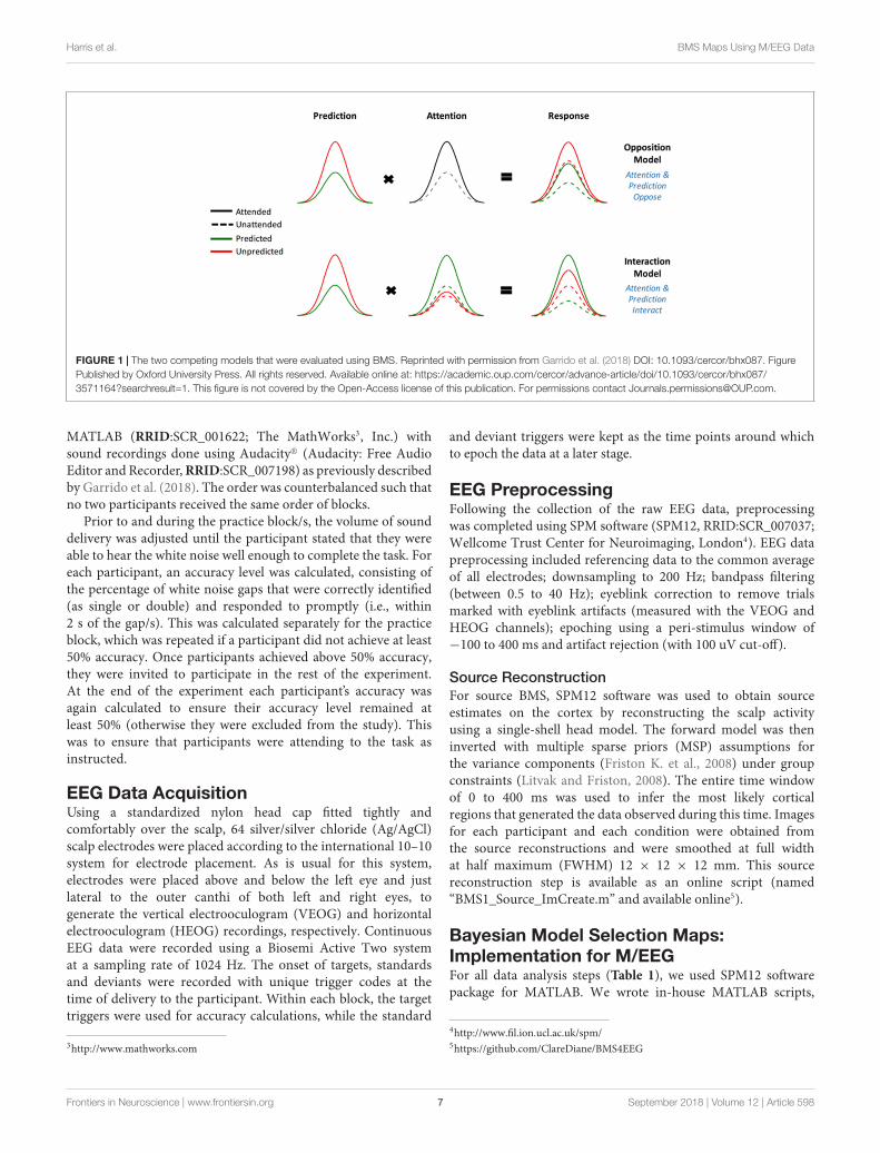
Experimental DesignThis experiment is a direct replication of that performed byGarrido et al. (2018), apart from the omission of a “dividedattention” condition. As they describe in greater detail intheir paper, Garrido et al. (2018) utilized a novel audio-spatialattention task during which attention and prediction wereorthogonally manipulated; this was done to evaluate the effectof surprise and attention in auditory processing (Garrido et al.,2018). The authors compared two models (shown in Figure 1)which may explain the effect attention has on the neuralresponses elicited by predicted and unpredicted events.

The original study supported the model in which attentionboosts neural responses to both predicted and unpredictedstimuli, called the Opposition Model (Garrido et al., 2018).Prediction attenuates neural activity, while attention enhancesthis activity. Since these effects occur in opposite directionsor have opposing effects, the researchers named the model(describing these effects) the Opposition Model. According tothis model, attention improves the accuracy of predictions byprecision weighting prediction errors more heavily. Thus, inlight of this model, attention and prediction work together (inopposite directions) to improve our ability to make more accuraterepresentations of the sensorium.

Our current study attempted to replicate the above-mentionedstudy with an independent dataset and employing the Bayesianmethods that resembled the original study as closely as possible.The only difference was that the divided-attention conditionwas not administered because it was not required for theimplementation and description of the BMS steps. It is hopedthat the detailed description of our methods, adapted from thoseoriginally developed for fMRI by Rosa et al. (2010), prove to beuseful for other EEG and/or MEG researchers. Furthermore, areplication study such as this one has the additional benefit ofbeing responsive to the persisting replication crisis that continuesto pose a significant problem for neuroscience and psychology(Hartshorne, 2012; Larson and Carbine, 2017; Szucs et al.,2017).

To this end we employed BMS to adjudicate between twocompeting hypotheses (see Figure 1), namely:

(1) Attention increases (boosts) neural responses to bothpredicted and unpredicted stimuli. This is formalized in

the Methods section and is then called Model One – theOpposition Model.

(2) Attention boosts neural responses to predicted stimulimore than it boosts responses to unpredicted stimuli. Thiscauses predicted attended stimuli to generate the highestneural responses, followed by attended unpredicted stimuli.This is formalized in the Methods section and is then calledModel Two – the Interaction Model.

ParticipantsTwenty-one healthy adults (aged between 19–64 years,M = 25.00 years, SD = 9.83, nine females) were recruitedvia the University of Queensland’s Psychology ResearchParticipation Scheme (SONA). Exclusion criteria includedany history of mental or neurological disease, any previoushead injury resulting in unconsciousness, or an age outside theprescribed range (18–65 years). All participants gave both writtenand verbal informed consent to both the study and to havingtheir de-identified data made available in publicly distributeddatabases. Participants completed practice blocks of stimuluspresentation prior to undergoing the EEG recording, in orderto enable them to withdraw if they found the task unpleasant orexcessively challenging. (No participants wished to withdraw.)Participants were monetarily compensated for their time. Thisstudy was approved by the University of Queensland HumanResearch Ethics Committee.

Task DescriptionParticipants wore earphones with inner-ear buds (Etymotic, ER3)and were asked to follow instructions on a computer screen.Participants were asked to pay attention to the sound stream ineither the left or the right ear (ignoring the sounds that werebeing played in the other ear). Gaussian white noise was playedto both ears and an oddball sequence was played to one ofthe ears. During a given block, participants were tasked withlistening carefully for gaps in the white noise on the side towhich they had been asked to attend. They were asked to pressa “1” on the numbered keyboard when they heard a single gap(lasting 90 ms) in the white noise, and a “2” when they hearda double gap (two 90 ms gaps separated by 30 ms of whitenoise). They were asked to ignore any tones played on boththe attended and the opposite ear. This task is described infurther detail, including pictorial representations, in Garrido et al.(2018).

Participants listened to eight different blocks, each 190 sin duration. Each block contained a total of 30 targets (15single gaps and 15 double gaps, randomly distributed acrossthe block, but never occurring within 2.5 s of each other andnever occurring at the same time as a tone). Throughout eachblock there were also 50-ms-long pure tones being played inone of the ears, with a 450 ms inter-stimulus interval. In eachblock there were two tones: the standard tone (either 500 Hz or550 Hz counterbalanced between blocks) that occurred 85% ofthe time, and the deviant (either 550 Hz or 500 Hz, the oppositeof the standard tone and counterbalanced across blocks) thatoccurred 15% of the time. All sound files were created using

Frontiers in Neuroscience | www.frontiersin.org 6 September 2018 | Volume 12 | Article 598

fnins-12-00598 September 26, 2018 Time: 18:13 # 7

Harris et al. BMS Maps Using M/EEG Data

FIGURE 1 | The two competing models that were evaluated using BMS. Reprinted with permission from Garrido et al. (2018) DOI: 10.1093/cercor/bhx087. FigurePublished by Oxford University Press. All rights reserved. Available online at: https://academic.oup.com/cercor/advance-article/doi/10.1093/cercor/bhx087/3571164?searchresult=1. This figure is not covered by the Open-Access license of this publication. For permissions contact Journals.permissions@OUP.com.

MATLAB (RRID:SCR_001622; The MathWorks3, Inc.) withsound recordings done using Audacity R© (Audacity: Free AudioEditor and Recorder, RRID:SCR_007198) as previously describedby Garrido et al. (2018). The order was counterbalanced such thatno two participants received the same order of blocks.

Prior to and during the practice block/s, the volume of sounddelivery was adjusted until the participant stated that they wereable to hear the white noise well enough to complete the task. Foreach participant, an accuracy level was calculated, consisting ofthe percentage of white noise gaps that were correctly identified(as single or double) and responded to promptly (i.e., within2 s of the gap/s). This was calculated separately for the practiceblock, which was repeated if a participant did not achieve at least50% accuracy. Once participants achieved above 50% accuracy,they were invited to participate in the rest of the experiment.At the end of the experiment each participant’s accuracy wasagain calculated to ensure their accuracy level remained atleast 50% (otherwise they were excluded from the study). Thiswas to ensure that participants were attending to the task asinstructed.

EEG Data AcquisitionUsing a standardized nylon head cap fitted tightly andcomfortably over the scalp, 64 silver/silver chloride (Ag/AgCl)scalp electrodes were placed according to the international 10–10system for electrode placement. As is usual for this system,electrodes were placed above and below the left eye and justlateral to the outer canthi of both left and right eyes, togenerate the vertical electrooculogram (VEOG) and horizontalelectrooculogram (HEOG) recordings, respectively. ContinuousEEG data were recorded using a Biosemi Active Two systemat a sampling rate of 1024 Hz. The onset of targets, standardsand deviants were recorded with unique trigger codes at thetime of delivery to the participant. Within each block, the targettriggers were used for accuracy calculations, while the standard

3http://www.mathworks.com

and deviant triggers were kept as the time points around whichto epoch the data at a later stage.

EEG PreprocessingFollowing the collection of the raw EEG data, preprocessingwas completed using SPM software (SPM12, RRID:SCR_007037;Wellcome Trust Center for Neuroimaging, London4). EEG datapreprocessing included referencing data to the common averageof all electrodes; downsampling to 200 Hz; bandpass filtering(between 0.5 to 40 Hz); eyeblink correction to remove trialsmarked with eyeblink artifacts (measured with the VEOG andHEOG channels); epoching using a peri-stimulus window of−100 to 400 ms and artifact rejection (with 100 uV cut-off).

Source ReconstructionFor source BMS, SPM12 software was used to obtain sourceestimates on the cortex by reconstructing the scalp activityusing a single-shell head model. The forward model was theninverted with multiple sparse priors (MSP) assumptions forthe variance components (Friston K. et al., 2008) under groupconstraints (Litvak and Friston, 2008). The entire time windowof 0 to 400 ms was used to infer the most likely corticalregions that generated the data observed during this time. Imagesfor each participant and each condition were obtained fromthe source reconstructions and were smoothed at full widthat half maximum (FWHM) 12 × 12 × 12 mm. This sourcereconstruction step is available as an online script (named“BMS1_Source_ImCreate.m” and available online5).

Bayesian Model Selection Maps:Implementation for M/EEGFor all data analysis steps (Table 1), we used SPM12 softwarepackage for MATLAB. We wrote in-house MATLAB scripts,

4http://www.fil.ion.ucl.ac.uk/spm/5https://github.com/ClareDiane/BMS4EEG

Frontiers in Neuroscience | www.frontiersin.org 7 September 2018 | Volume 12 | Article 598

fnins-12-00598 September 26, 2018 Time: 18:13 # 8

Harris et al. BMS Maps Using M/EEG Data

TABLE 1 | Step-by-step summary of method.

Task: Suggested steps:

Saving the correct spm_spm_vb.m files 1. Find and open the SPM12 folder on your computer.2. Find the spm_spm_vb.m script in that folder, and rename this to spm_spm_vb_fMRI.m. Then add thespm_spm_vb_ST.m and spm_spm_vb_source.m scripts (saved in the associated Github repository) to yourSPM12 folder.3. Before undertaking either the spatiotemporal BMS or source BMS steps, rename the currently relevant scriptfrom the above step to spm_spm_vb.m. Once you have finished the BMS steps, rename the script back to itsoriginal name, to re-identify it as being for either the spatiotemporal (‘spm_spm_vb_ST.m’) or source BMS(‘spm_spm_vb_source.m’). In this way, you will keep track of which spm_spm_vb.m script to use for whicheverBMS steps you are about to do.

Creating spatiotemporal (“scalp”) PPMs: 1. BMS script 1: Change the file paths to reflect the location of ERP data.2. Run BMS script 1: BMS1_ST_ImCreate.m.3. Ensure the correct spm_spm_vb.m file is saved in SPM12 folder.4. Run BMS script 2: BMS2_ModelSpec_VB.m.5. Run BMS script 3: BMS3_PPMs.m. Threshold is set to 0.75 and adjustable.

Creating source PPMs: 1. BMS script 1: Change the file paths to reflect location of source reconstructed images.2. Run BMS script 1: BMS1_Source_ImCreate.m.3. Ensure the correct spm_spm_vb.m file is saved in SPM12 folder.4. Run BMS script 2: BMS2_ModelSpec_VB.m.5. Replace NaNs with zeros in the LogEv.nii files: BMS2b_Source_NaNtoZeros.m.6. Run BMS script 3: BMS3_PPMs.m. Adjust probability threshold as desired.

integrated with SPM12 and now available online6. Copies ofthe scripts are also given in the Supplementary Material.The online scripts are divided into three BMS scripts. Inthe first script (BMS1_ST_ImCreate.m for spatiotemporal BMSand BMS1_Source_ImCreate.m for source BMS), we call thepreprocessed EEG data and then create images for every trial,for every condition, and for every participant. The secondscript (BMS2_ModelSpec_VB.m) specifies the hypotheses andimplements VB (as described in the Theory section). The lastscript (BMS3_PPMs.m) then creates PPMs.

In the model specification and VB script(BMS2_ModelSpec_VB.m), we changed individual participants’data file structures in order to match the format thatSPM typically requires to read fMRI data. This is done byfirst loading the relevant file path and then changing the filestructure. Once these newly structured files had been saved,we next specified the models to be compared: this was done byassigning covariate weights to describe both models (please seethe instructions contained within BMS2_ModelSpec_VB.m onGithub). The Opposition Model was assigned weights of [1, 2,2, and 3] for the unattended predicted, attended predicted andunattended unpredicted, and attended unpredicted, respectively.The Interaction Model was assigned weights of [1, 4, 2, and 3] forthe same conditions.

These covariate weights essentially describe the assumedrelationship between the different conditions according to a givenmodel. For example, using [1, 2, 2, and 3] as employed inthe Opposition Model, means that according to the OppositionModel, the unattended predicted condition (the first conditionwith an assigned weight of 1) evokes the smallest activity, whereasthe attended unpredicted (the fourth condition with a weightof 3) has the greater activity, and both attended predicted andunattended unpredicted (second and third conditions with an

6https://github.com/ClareDiane/BMS4EEG

equal weight of 2) are in between the former two conditions andindistinguishable in magnitude from each other.

We then created log-evidence images, representing thelog-model evidences, for both models (separately), for everyparticipant (individually) at every voxel. In the case ofspatiotemporal (scalp-level) BMS, each voxel was representativeof a specific spatiotemporal location within the peristimulustime window (0 to 400 ms) and topologically across the scalp,such that the first two dimensions of the voxel refer to thespace across the scalp and the third dimension is time (asshown in Figure 2). Conversely, in the source BMS (whichbegan with the source reconstruction steps described above),each voxel was representative of an inferred location in three-dimensional source space. Once log-evidence images had beencreated, these were smoothed with a 1 mm half-width Gaussiankernel.

In summary, one can create PPMs or log evidence maps insensor or source space. In sensor space, this involves creatinga two-dimensional image over the scalp surface and equippingthe space with a peristimulus time dimension. This createsPPMs over the scalp surface and peristimulus time, enabling oneto identify regionally and temporally specific effects due to aparticular model, relative to other contrasts. Alternatively, onecan create three-dimensional PPMs in source space, followingsource reconstruction.

The core SPM script that allows VB to be used on fMRIdata is named spm_spm_vb.m and is found in the SPM12package, downloadable from the SPM site. This core script wasedited in order to adapt the VB method for EEG, as follows.Changes were made such that different data structures couldbe read in the same way that fMRI data would usually beread. Furthermore, high-pass filtering steps were removed asthese only apply to low-frequency drifts associated with fMRIdata. The specific changes made between the original scriptand the altered one to be used for spatiotemporal BMS are

Frontiers in Neuroscience | www.frontiersin.org 8 September 2018 | Volume 12 | Article 598

fnins-12-00598 September 26, 2018 Time: 18:13 # 9

Harris et al. BMS Maps Using M/EEG Data

FIGURE 2 | Scalp Posterior Probability Maps of the two competing models over space and time. (The scalp images include the participant’s nose, pointing upward,and ears, visible as if viewed from above.) These maps display all posterior probabilities exceeding 75% over space and time for both models. The left sides of bothpanels (A,C) both depict the temporal information, showing the model probabilities at each point in time from 0 ms (when the tone was played, at the top of thediagrams) to 400 ms after the stimulus presentation (at the bottom of the diagram), across the surface of the scalp (which traverses the width of the panels). Theright sides (B,D) show the spatial locations of the probability clusters which exceeded the threshold of 75% probability. Panels (B) and (D) were generated using thespatiotemporal visualization tools developed by Jeremy Taylor. These tools are available at: https://github.com/JeremyATaylor/Porthole.

accessible online (goo.gl/ZVhPT7). For the source BMS steps,the same changes were left in place as outlined above, and inaddition, the required minimum cluster size was changed from16 to 0 voxels to allow for visualization of all clusters of anysize. The specific differences between the original and sourceBMS versions of the spm_spm_vb script are accessible online(goo.gl/WXAo67).

In the final step (BMS3_PPMs.m), the SPM Batch Editor wasused to apply a RFX approach to the group model evidencedata in a voxel-wise manner, thus translating the log-evidenceimages from the previous step into PPMs (similar to how Rosaet al. (2010) have produced PPMs previously for fMRI data).The maps, displayed in the Figures 2–4, were generated byselecting threshold probabilities of 75% for the spatiotemporalmaps (Figure 2) and 50% for the source maps (Figures 3 and4). This threshold can be adjusted by the user. EPMs can alsobe displayed by selecting the relevant setting in the final script(please see the instructions on Github).

RESULTS

The raw dataset for this study can be found; on Figshare(EEG_Auditory_Oddball_Raw_Data repository7; Harris et al.,2018a).

The preprocessed dataset for this study can also befound on Figshare (EEG_Auditory_Oddball_Preprocessed_Datarepository8; Harris et al., 2018b).

Scalp – SpatiotemporalFigure 2 shows scalp (spatiotemporal) PPMs of the twocompeting models over space and time. These maps display allposterior probabilities exceeding 75% over space and time forboth models. As can be seen in the figure, spatiotemporal BMSresults revealed that Model One (the Opposition Model) was

7https://figshare.com/s/1ef6dd4bbdd4059e38918https://figshare.com/s/c6e1f9120763c43e6031

Frontiers in Neuroscience | www.frontiersin.org 9 September 2018 | Volume 12 | Article 598

fnins-12-00598 September 26, 2018 Time: 18:13 # 10

Harris et al. BMS Maps Using M/EEG Data

FIGURE 3 | Source Posterior Probability Map for the Opposition Model (thatis, reconstructed images representing the model inference at the group levelfor this model), thresholded at > 50% posterior probability. (A) View from theleft side. (B) View from the left side, from the posterior (back) end. (C) Viewfrom the right side. (D) View from above.

FIGURE 4 | Source Posterior Probability Map for the Interaction Model (thatis, reconstructed images representing the model inference at the group levelfor this model), thresholded at > 50% posterior probability. (A) View from theleft side. (B) View from the left side, from the posterior (back) end. (C) Viewfrom the right side. (D) View from above.

by and large the superior model. The Opposition Model hadmodel probabilities exceeding 75% across the majority of latertime points (with most significant clusters between 225–360 ms),and over most frontocentral and bilateral channel locations, asshown in (A). On the other hand, as shown in (C), the Interaction

FIGURE 5 | Comparison of the posterior probabilities for the two modelsat the location of the highest-probability cluster of the Opposition Model (left)and the location of the highest-probability cluster of the Interaction Model(right). The left supramarginal gyrus cluster, which was the highest probabilitycluster for the Opposition Model (left), was located at Montreal NeurologicalInstitute (MNI) coordinates (62, –42, 30), while the left inferior parietal lobecluster, which was the highest probability cluster for the Interaction Model,was located at MNI coordinates (–54, –32, 46).

Model did have over 75% model probability centrally between175–185 ms, which is within the mismatch negativity (MMN)time window. These findings replicate those of Garrido et al.(2018), and strongly support the implications discussed in greatdepth in that paper.

SourceAs shown in Figures 3, 4, and 5, source BMS results also favoredthe Opposition Model, with higher model probability over theleft supramarginal gyrus (with 91% model probability over arelatively large cluster, KE = 6115), the right superior temporalgyrus (with 87% model probability over a cluster with KE = 5749)as well as over parts of the left inferior parietal lobe, right inferiorparietal lobe and left postcentral gyrus. Having said this, theInteraction Model also had two large clusters, albeit with lowermodel probabilities compared to the Opposition Model’s highest-probability clusters: specifically, the Interaction Model had acluster of size KE = 6346 over the left inferior parietal lobe anda cluster of size KE = 5353 over the right inferior parietal lobe(with 74% model probability in both places).

Figures 3 and 4 show that different brain regions are likely toperform different computations best described by the Oppositionand Interaction Models, respectively. Furthermore, Figure 5compares the magnitude of the calculated posterior probabilities,at the locations of the highest probability cluster for both models.The possible functional reasons for the different anatomicallocations that emerge for the two different models may be aninteresting subject for future study, but fall outside the scope ofthis methods paper. In any case, the usefulness of this probabilitymapping approach illustrated in Figures 2, 3, and 4, lies in theability to pinpoint where and when given computations are likelyto be performed in the brain.

Frontiers in Neuroscience | www.frontiersin.org 10 September 2018 | Volume 12 | Article 598

fnins-12-00598 September 26, 2018 Time: 18:13 # 11

Harris et al. BMS Maps Using M/EEG Data

DISCUSSION

This paper shows how to use RFX BMS mapping methods forM/EEG data analysis. This method was originally developed forfMRI by Rosa et al. (2010), and provides a way of displaying theprobabilities of different cognitive models at different timepointsand brain locations, given a neuroimaging dataset. We aimed toprovide an in-depth explanation, written in a didactical manner,of the BMS and posterior probability mapping steps that weresuccessfully used by Garrido et al. (2018) in their recent EEGpaper.

Being a Bayesian approach to hypothesis-testing, the methoddescribed here provides multiple advantages over frequentistinference methods. The first of these advantages is that VB allowsfor comparisons between non-nested models. Consequently, itis especially useful in the context of model-based neuroimaging(Montague et al., 2004; O’Doherty et al., 2007; Rosa et al.,2010; Garrido et al., 2018). Another advantage is that theprobability of the null hypothesis itself can be assessed(instead of simply being, or failing to be, rejected). A finaladvantage is that, although only two models were comparedhere, the same method can also be applied to any arbitrarynumber of models. For example, the analyses described herecould proceed slightly differently, based on the same databut introducing another (or multiple other) model/s againstwhich to compare the Opposition and Interaction Models.Potentially, any number of theoretically motivated models couldbe considered. Considering all of these advantages, the methoddescribed here should prove useful in a wide variety of M/EEGexperiments.

In summary, we have shown here how to adapt BMS maps,originally developed for fMRI data by Rosa et al. (2010),to M/EEG data analysis. It is hoped that the reporting ofanalytical methods such as these, as well as the availabilityof all the code and dataset, will not only contribute tothe Open Science movement, but may also encourage otherresearchers to adopt this novel M/EEG data analysis methodin a way that is useful for addressing their own neurosciencequestions. We postulate that the use of this Bayesian modelmapping of M/EEG data to adjudicate between competingcomputational models in the brain, both at the scalp and

source level, will be a significant advancement in the field ofM/EEG neuroimaging and may provide new insights in cognitiveneuroscience.

AUTHOR CONTRIBUTIONS

MG designed the study and the analysis methods. ER wrote thecode and adapted SPM scripts from fMRI to M/EEG. CH and RRcollected and analyzed the data, and organized the data and codefor sharing. CH wrote the first draft of the manuscript. ER, RR,and MG edited the manuscript.

FUNDING

This work was funded by the Australian Research CouncilCenter of Excellence for Integrative Brain Function (ARCCenter Grant CE140100007) and a University of QueenslandFellowship (2016000071) to MG. RR and CH were bothsupported by Research Training Program scholarships awardedby The University of Queensland.

ACKNOWLEDGMENTS

We thank the participants for their time. We are grateful to MariaRosa for helpful advice regarding source BMS steps, and to thetwo reviewers, whose helpful comments and suggestions led tosignificant improvements in the paper. We also thank JessicaMcFadyen for help with preprocessing, Ilvana Dzafic for helpwith EEG data acquisition, and Jeremy Taylor for sharing toolsfor visualizing spatiotemporal images (shown in panels (B) and(D) in Figure 2).

SUPPLEMENTARY MATERIAL

The Supplementary Material for this article can be foundonline at: https://www.frontiersin.org/articles/10.3389/fnins.2018.00598/full#supplementary-material

REFERENCESAkaike, H. (1980). Likelihood and the Bayes procedure. Trab. Estad. Investig. Oper.

31, 143–166. doi: 10.1007/BF02888350Bayes, T., and Price, R. (1763). An essay towards solving a problem in the doctrine

of chances. by the late Rev. Mr. Bayes, frs communicated by Mr. Price, in a letterto John Canton, amfrs. Philos. Trans. 168, 370–418. doi: 10.1098/rstl.1763.0053

Beal, M., and Ghahramani, Z. (2003). “The variational Bayesian EM algorithmsfor incomplete data: with application to scoring graphical model structures,”in Bayesian Statistics 7, eds J. Bernardo, M. Bayarri, J. Berger, and A. Dawid(Cambridge: Cambridge University Press).

Beal, M. J. (2003). Variational Algorithms for Approximate Bayesian Inference.London: University of London, 281.

Blei, D. M., Kucukelbir, A., and McAuliffe, J. D. (2017). Variational inference: areview for statisticians. J. Am. Stat. Assoc. 112, 859–877. doi: 10.1080/01621459.2017.1285773

Carter, T. (2007). An Introduction to Information Theory and Entropy. Santa Fe,NM: Complex Systems Summer School.

Connor, J. T., Elm, J. J., Broglio, K. R., and Esett and Adapt-It Investigators (2013).Bayesian adaptive trials offer advantages in comparative effectiveness trials: anexample in status epilepticus. J. Clin. Epidemiol. 66, S130–S137. doi: 10.1016/j.jclinepi.2013.02.015

Dayan, P., Hinton, G. E., Neal, R. M., and Zemel, R. S. (1995). Thehelmholtz machine. Neural Comput. 7, 889–904. doi: 10.1162/neco.1995.7.5.889

Dienes, Z. (2016). How Bayes factors change scientific practice. J. Math. Psychol.72, 78–89. doi: 10.1016/j.jmp.2015.10.003

Dunson, D. B. (2001). Commentary: practical advantages of Bayesian analysis ofepidemiologic data. Am. J. Epidemiol. 153, 1222–1226. doi: 10.1093/aje/153.12.1222

Feldman, H., and Friston, K. (2010). Attention, uncertainty, and free-energy. Front.Hum. Neurosci. 4, 215–238. doi: 10.3389/fnhum.2010.00215

Feynman, R. P., and Brown, L. M. (1942). Feynman’s Thesis: A New Approach toQuantum Theory. Hackensack, NJ: World Scientific.

Feynman, R. P., Hibbs, A. R., and Styer, D. F. (2010). QuantumMechanics and PathIntegrals. New York, NY: Courier Corporation.

Frontiers in Neuroscience | www.frontiersin.org 11 September 2018 | Volume 12 | Article 598

fnins-12-00598 September 26, 2018 Time: 18:13 # 12

Harris et al. BMS Maps Using M/EEG Data

Friston, K. (2007). APPENDIX 1 – Linear Models and Inference. StatisticalParametric Mapping. London: Academic Press, 589–591.

Friston, K. (2012). The history of the future of the Bayesian brain. Neuroimage 62,1230–1233. doi: 10.1016/j.neuroimage.2011.10.004

Friston, K., Harrison, L., Daunizeau, J., Kiebel, S., Phillips, C., Trujillo-Barreto, N.,et al. (2008). Multiple sparse priors for the M/EEG inverse problem.Neuroimage39, 1104–1120. doi: 10.1016/j.neuroimage.2007.09.048

Friston, K., Kiebel, S., Garrido, M., and David, O. (2007). CHAPTER 42 – DynamicCausal Models for EEG. Statistical Parametric Mapping. London: AcademicPress, 561–576. doi: 10.1016/B978-012372560-8/50042-5

Friston, K., and Penny, W. (2003). Posterior probability maps andSPMs. Neuroimage 19, 1240–1249. doi: 10.1016/S1053-8119(03)00144-7

Friston, K., and Penny, W. (2007). CHAPTER 23 – Posterior Probability Maps.Statistical Parametric Mapping. London: Academic Press, 295–302. doi: 10.1016/B978-012372560-8/50023-1

Friston, K. J., Trujillo-Barreto, N., and Daunizeau, J. (2008). DEM: a variationaltreatment of dynamic systems. Neuroimage 41, 849–885. doi: 10.1016/j.neuroimage.2008.02.054

Garrido, M., Rowe, E., Halasz, V., and Mattingley, J. (2018). Bayesianmapping reveals that attention boosts neural responses to predicted andunpredicted stimuli. Cereb. Cortex 28, 1771–1782. doi: 10.1093/cercor/bhx087

Harris, C. D., Rowe, E. G., Randeniya, R., and Garrido, M. I. (2018a).Bayesian Model Selection Maps for Group Studies Using M/EEG Data:EEG_Auditory_Oddball_Raw_Data. Figshare. Available at: https://figshare.com/s/1ef6dd4bbdd4059e3891

Harris, C. D., Rowe, E. G., Randeniya, R., and Garrido, M. I. (2018b).Bayesian Model Selection Maps for group studies using M/EEG data:EEG_Auditory_Oddball_Preprocessed_Data. Figshare. Available at: https://figshare.com/s/c6e1f9120763c43e6031

Hartshorne, J. (2012). Tracking replicability as a method of post-publicationopen evaluation. Front. Comput. Neurosci. 6, 70–83. doi: 10.3389/fncom.2012.00008

Hohwy, J. (2013). The Predictive Mind. Oxford: Oxford University Press.doi: 10.1093/acprof:oso/9780199682737.001.0001

Horn, R. (1987). Statistical methods for model discrimination. Applications togating kinetics and permeation of the acetylcholine receptor channel. Biophys.J. 51, 255–263. doi: 10.1016/S0006-3495(87)83331-3

Kass, R. E., and Raftery, A. E. (1995). Bayes factors. J. Am. Stat. Assoc. 90, 773–795.doi: 10.1080/01621459.1995.10476572

Kullback, S., and Leibler, R. A. (1951). On information and sufficiency. Ann. Math.Stat. 22, 79–86. doi: 10.1214/aoms/1177729694

Lappalainen, H., and Miskin, J. W. (2000). “Ensemble learning,” in Advances inIndependent Component Analysis, ed. M. Girolami (Berlin: Springer-Verlag).

Larson, M. J., and Carbine, K. A. (2017). Sample size calculations inhuman electrophysiology (EEG and ERP) studies: a systematic review andrecommendations for increased rigor. Int. J. Psychophysiol. 111, 33–41.doi: 10.1016/j.ijpsycho.2016.06.015

Litvak, V., and Friston, K. (2008). Electromagnetic source reconstructionfor group studies. Neuroimage 1490–1498. doi: 10.1016/j.neuroimage.2008.06.022

McAleer, M. (1995). The significance of testing empirical non-nested models.J. Econom. 67, 149–171. doi: 10.1016/0304-4076(94)01631-9

Meinert, C. L. (2012). Frequentist vs. Bayesian Analysis. Hoboken, NJ: John Wiley& Sons, Inc. doi: 10.1002/9781118422878.ch138

Mohammad-Djafari, A. (2002). Bayesian inference for inverse problems. AIP Conf.Proc. 617, 477–496. doi: 10.1063/1.1477067

Montague, P. R., Hyman, S. E., and Cohen, J. D. (2004). Computational rolesfor dopamine in behavioural control. Nature 431, 760–767. doi: 10.1038/nature03015

Neal, R. (1998). Annealed Importance Sampling (Technical Report 9805 (revised)).Toronto, ON: University of Toronto.

Needham, C. J., Bradford, J. R., Bulpitt, A. J., and Westhead, D. R. (2007). A primeron learning in Bayesian networks for computational biology. PLoS Comput.Biol. 3:e129. doi: 10.1371/journal.pcbi.0030129

Neyman, J., and Pearson, E. S. (1933). On the problem of the most efficient testsof statistical hypotheses. Proc. R. Soc. Lond. A Math. Phys. Sci. 231, 289–337.doi: 10.1098/rsta.1933.0009

O’Doherty, J. P., Hampton, A., and Kim, H. (2007). Model-based fMRI and itsapplication to reward learning and decision making. Ann. N.Y. Acad. Sci. 1104,35–53. doi: 10.1196/annals.1390.022

Penny, W., Flandin, G., and Trujillo-Barreto, N. (2007a). Bayesian comparison ofspatially regularised general linear models. Hum. Brain Mapp. 28, 275–293.

Penny, W., Kiebel, S., and Friston, K. (2007b). CHAPTER 24 – Variational Bayes.Statistical Parametric Mapping. London: Academic Press, 303–312. doi: 10.1016/B978-012372560-8/50024-3

Penny, W., Kiebel, S., and Friston, K. (2003). Variational Bayesian inferencefor fMRI time series. Neuroimage 19, 727–741. doi: 10.1016/S1053-8119(03)00071-5

Penny, W., and Sengupta, B. (2016). Annealed importance sampling for neuralmass models. PLoS Comput. Biol. 12:e1004797. doi: 10.1371/journal.pcbi.1004797

Penny, W. D. (2012). Comparing dynamic causal models using AIC. BIC and freeenergy. Neuroimage 59, 319–330. doi: 10.1016/j.neuroimage.2011.07.039

Penny, W. D., and Ridgway, G. R. (2013). Efficient posterior probability mappingusing Savage-Dickey ratios. PLoS One 8:e59655. doi: 10.1371/journal.pone.0059655

Penny, W. D., Stephan, K. E., Mechelli, A., and Friston, K. J. (2004). Comparingdynamic causal models. Neuroimage 22, 1157–1172. doi: 10.1016/j.neuroimage.2004.03.026

Rissanen, J. (1978). Modeling by shortest data description. Automatica 14,465–471. doi: 10.1016/0005-1098(78)90005-5

Rosa, M., Bestmann, S., Harrison, L., and Penny, W. (2010). Bayesian modelselection maps for group studies. Neuroimage 49, 217–224. doi: 10.1016/j.neuroimage.2009.08.051

Schwarz, G. (1978). Estimating the dimension of a model. Ann. Stat. 6, 461–464.doi: 10.1214/aos/1176344136

Shannon, C. E. (1948/2001). A Mathematical Theory of Communication:ACM SIGMOBILE Mobile Computing and Communications Review, Vol. 5.New York, NY: ACM, 3–55.

Stephan, K. E., Penny, W. D., Daunizeau, J., Moran, R. J., and Friston, K. J.(2009). Bayesian model selection for group studies. Neuroimage 46, 1004–1017.doi: 10.1016/j.neuroimage.2009.03.025

Szucs, D., Ioannidis, J. P. A., and Wagenmakers, E.-J. (2017). Empirical assessmentof published effect sizes and power in the recent cognitive neuroscienceand psychology literature. PLoS Biol. 15:e2000797. doi: 10.1371/journal.pbio.2000797

Trippa, L., Lee, E. Q., Wen, P. Y., Batchelor, T. T., Cloughesy, T., Parmigiani, G.,et al. (2012). Bayesian adaptive randomized trial design for patients withrecurrent glioblastoma. J. Clin. Oncol. 30, 3258–3263. doi: 10.1200/JCO.2011.39.8420

Vallverdú, J. (2008). The false dilemma: Bayesian vs. Frequentist. arXiv [Preprint].arXiv:0804.0486

Conflict of Interest Statement: The authors declare that the research wasconducted in the absence of any commercial or financial relationships that couldbe construed as a potential conflict of interest.

Copyright © 2018 Harris, Rowe, Randeniya and Garrido. This is an open-accessarticle distributed under the terms of the Creative Commons Attribution License(CC BY). The use, distribution or reproduction in other forums is permitted, providedthe original author(s) and the copyright owner(s) are credited and that the originalpublication in this journal is cited, in accordance with accepted academic practice.No use, distribution or reproduction is permitted which does not comply with theseterms.

Frontiers in Neuroscience | www.frontiersin.org 12 September 2018 | Volume 12 | Article 598

Minerva Access is the Institutional Repository of The University of Melbourne

Author/s:Harris, CD;Rowe, EG;Randeniya, R;Garrido, MI

Title:Bayesian Model Selection Maps for Group Studies Using M/EEG Data

Date:2018-09-28

Citation:Harris, C. D., Rowe, E. G., Randeniya, R. & Garrido, M. I. (2018). Bayesian Model SelectionMaps for Group Studies Using M/EEG Data. FRONTIERS IN NEUROSCIENCE, 12, https://doi.org/10.3389/fnins.2018.00598.

Persistent Link:http://hdl.handle.net/11343/250080

License:CC BY