bayesian inference for simple problems

Bayesian Inference for Simple Problems

Simon Jackman

Stanford Universityhttp://jackman.stanford.edu/BASS

February 11, 2012

Simon Jackman (Stanford) Bayesian Inference for Simple Problems February 11, 2012 1 / 30

Conjugacy

Bayes Rule says p(h|y) ∝ p(h)p(y|h)Mantra: ‘‘Posterior is proportional to prior times likelihood’’

This math easy to do when we use prior densities that are conjugatewith respect to the likelihood p(y|h).


Conjugacy

Definition 1.2 (p15 BASS): Suppose a prior density p(h) belongs to a classof parametric densities, F . Then the prior density is said to be conjugatewith respect to a likelihood p(y|h) if the posterior density p(h|y) is also inF .

Up until the Markov-chain Monte Carlo revolution in the 1990s,Bayesian inference was almost all done with

conjugate priorssimple problems; e.g., rates and proportions (Bernoulli trials,coin-flipping), counts (Poisson), means, variances and regression(normal data).

Bayes estimates such as the mean of the posterior density E(h|y)have a simple mathematical form; can be computed ‘‘by hand’’; are‘‘precision-weighted averages’’ of estimates based on the prior andon the data.


Example: coin flipping (p50)

yi ∈ {0,1}, exchangeable

unknown success probability h ∈ [0,1],

data: yiiid∼ Bernoulli(h), i = 1, . . . , n

r ∼ Binomial(h; n), r =∑

yi.

binomial likelihood p(r|h):(nr

)hr(1 - h)n-r

What prior density p(h) is conjugate wrt the likelihood p(r|h)?That is, what form does p(h) have to be such thatp(h|r, n) ∝ p(r|h, n)p(h) is of the same form?

Answer: the Beta density is conjugate wrt a binomial likelihood.


Beta density

A prior density for h ∈ [0,1] must have the properties:1 p(h) ≥ 0, h ∈ [0,1].2∫ 1

0 p(h)dh = 1.

A conjugate prior must also have the property thatp(h|r, n) ∝ p(r|h, n)p(h) is of the same form as p(h).

Definition

Beta density:

p(h;α, b) =C(α+ b)

C(α)C(b)hα-1(1 - h)b-1,

where h ∈ [0,1], α, b > 0 and C(z) =∫

L

0 tz-1exp(-t)dt is the Gammafunction (Definition B.19).


Beta density

p(h;α, b) =C(α+ b)

C(α)C(b)hα-1(1 - h)b-1

Note that the leading terms involving the Gamma functions do notinvolve h: p(h;α, b) ∝ hα-1(1 - h)b-1.

A uniform density on [0,1] is a special case of the Beta density,arising when α = b = 1.

Symmetric densities with a mode/mean/median at .5 are generatedwhen α = b for α, b > 1.

the mean, E(h) =α

α+ b

the mode:α - 1

α+ b - 2

the variance:αb

(α+ b)2(α+ b + 1)


Beta density

0.0 0.2 0.4 0.6 0.8 1.0

α = 1, β = 1

0.0 0.2 0.4 0.6 0.8 1.0

α = 1, β = 2

0.0 0.2 0.4 0.6 0.8 1.0

α = 2, β = 1

0.0 0.2 0.4 0.6 0.8 1.0

α = 2, β = 2

0.0 0.2 0.4 0.6 0.8 1.0

α = 3, β = 3

0.0 0.2 0.4 0.6 0.8 1.0

α = 50, β = 50

0.0 0.2 0.4 0.6 0.8 1.0

α = 5, β = 1

0.0 0.2 0.4 0.6 0.8 1.0

α = 1, β = 5

0.0 0.2 0.4 0.6 0.8 1.0

α = 1, β = 9

0.0 0.2 0.4 0.6 0.8 1.0

α = 3, β = 27

0.0 0.2 0.4 0.6 0.8 1.0

α = 10, β = 90

0.0 0.2 0.4 0.6 0.8 1.0

α = 0.5, β = 0.5


Conjugacy of the Beta wrt the Binomial Likelihood

TheoremConjugacy of Beta Prior, Binomial Data. Given a binomial likelihood over rsuccesses in n Bernoulli trials, each independent conditional on anunknown success parameter h ∈ [0,1], i.e.,

L(h; r, n) =(

nr

)hr(1 - h)n-r

then the prior density p(h) = Beta(α, b) is conjugate with respect to thebinomial likelihood, generating the posterior densityp(h|r, n) = Beta(α+ r, b + n - r).

Shorthand:h ∼ Beta(α, b), r ∼ Binomial(h, n)⇒ h|r, n ∼ Beta(α+ r, b + n - r).


Conjugacy of the Beta wrt the Binomial Likelihood

Proof of Proposition: Conjugacy of Beta Prior, Binomial Data.By Bayes Rule,

p(h|r, n) =L(h; r, n)p(h)∫ 1

0 L(h; r, n)p(h)dh∝ L(h; r, n)p(h)

Ignoring terms that do not depend on h,

p(h|r, n) ∝ hr(1 - h)n-r︸︷︷︸likelihood

hα-1(1 - h)b-1︸︷︷︸prior

= hr+α-1(1 - h)n-r+b-1

which is the kernel of a Beta density. That is,p(h|r, n) = chr+α-1(1 - h)n-r+b-1 where c is the normalizing constant

C(n + α+ b)

C(r + α)C(n - r + b),

In other words, h|r, n ∼ Beta(α+ r, b + n - r).Simon Jackman (Stanford) Bayesian Inference for Simple Problems February 11, 2012 9 / 30

Interpretation of Conjugacy in Data-Equivalent Terms

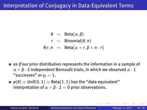
h ∼ Beta(α, b)

r ∼ Binomial(h, n)

h|r, n ∼ Beta(α+ r, b + n - r)

as if our prior distribution represents the information in a sample ofα+ b - 2 independent Bernoulli trials, in which we observed α - 1‘‘successes’’ or yi = 1.

p(h) ≡ Unif(0,1) ≡ Beta(1,1) has the ‘‘data equivalent’’interpretation of α+ b - 2 = 0 prior observations.


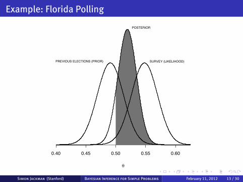
Example: Florida Polling

Florida poll, March 2000, voting intentions for the November 2000presidential election.n = 621. Bush 45% (n = 279), Gore 37% (230), Buchanan 3% (19)and undecided 15% (93).For simplicity, we ignore the undecided and Buchanan vote share,leaving Bush with 55% of the two-party vote intentions, and Gorewith 45%, and n = 509 respondents expressing a preference for thetwo major party candidates.We assume that the survey responses are independent, and (perhapsunrealistically) that the sample is a random sample of Floridianvoters.Thus, the binomial likelihood is (ignoring constants that do notdepend on h),

p(r|h, n) ∝ h279(1 - h)509-279.

The maximum likelihood estimate of h ishMLE = r/n = 279/509 = .548



Prior information from previous elections.Forecasting model produces a forecast of Bush vote share of 49.1%,with a standard error of 2.2 percentage points.Convert this to a Beta density: we seek values for α and b such that

E(h;α, b) = α/(α+ b) = .491

V(h;α, b) =αb

(α+ b)2(α+ b + 1)= .0222

which yields a system of equations in two unknowns.Solving yields

α = 515.36~.491 = 253.04,

b = 515.36~(1 - .491) = 262.32.

information in the previous elections is equivalent to having rananother poll with n ≈ 515 in which r ≈ 253 respondents said theywould vote for the Republican presidential candidate.



θ

0.40 0.45 0.50 0.55 0.60

POSTERIOR

SURVEY (LIKELIHOOD)PREVIOUS ELECTIONS (PRIOR)


Bayes Estimate as a Convex Combination of Prior andData

Consider a Bayes estimate such as the posterior mean:

E(h|r, n) =α*

α* + b*=

α+ rα+ b + n

=n0h0 + nh

n0 + n

where h = r/n is the maximum likelihood estimate of h, n0 = α+ b andh0 = α/(α+ b) = E(h) is the mean of the prior density for h.Alternatively,

E(h|r, n) = ch0 + (1 - c)h

where c = n0/(n0 + n), and since n0, n > 0, c ∈ [0,1]. Alternatively,

E(h|r, n) = h + c(h0 - h).

That is, a Bayes estimate of h --- is a weighted average of the prior meanh0 and the maximum likelihood estimate h.


Conjugate analysis of normal data

We first consider the simple case of normal data, with unknown mean land known variance r2:

yiiid∼ N(l, r2)

Likelihood:

p(y1, . . . , yn) =n∏

i=1

1√2pr2

exp[-(yi - l)2

2r2

]Conjugacy: we seek a prior for l, p(l), s.t. the posterior

p(l|y1, . . . , yn) ∝ p(y1, . . . , yn|l, r2)p(l)

is in the same class as p(l).


Conjugate analysis of normal data

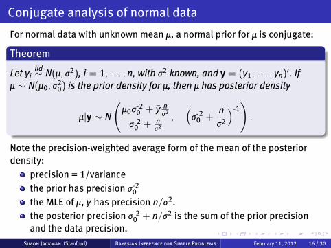
For normal data with unknown mean l, a normal prior for l is conjugate:

Theorem

Let yiiid∼ N(l, r2), i = 1, . . . , n, with r2 known, and y = (y1, . . . , yn)

′. Ifl ∼ N(l0, r2

0) is the prior density for l, then l has posterior density

l|y ∼ N

(l0r-20 + y n

r2

r-20 + nr2

,(

r-20 +nr2

)-1).

Note the precision-weighted average form of the mean of the posteriordensity:

precision = 1/variancethe prior has precision r-20

the MLE of l, y has precision n/r2.the posterior precision r-20 + n/r2 is the sum of the prior precisionand the data precision.


Conjugate analysis, normal data, mean and varianceunknown

Same model as in previous section: yiiid∼ N(l, r2).

Likelihood:

p(y1, . . . , yn) =n∏

i=1

1√2pr2

exp[-(yi - l)2

2r2

]

Parameters: a vector h = (l, r2)′, l ∈ R, r2 ∈ R+; i.e.,h ∈ H = R~R+.

Prior: it is easier to obtain a conjugate prior if we factor the jointdensity over h into the product of a conditional density for l given r2

and a marginal density for r2; i.e., p(h) = p(l, r2) = p(l|r2)p(r2).


Conjugate analysis, normal data, mean and varianceunknown

Prior: p(l, r2) = p(l|r2)p(r2) where

l|r2 ∼ N(l0, r2/n0)

r2 ∼ Inverse-Gamma(m0/2, m0 r20/2)

where

l0 = E(l|r2) = E(l) is the mean of the prior density for l

r2/n0 is the variance of the prior density for l, conditional on r2, withn0 interpretable as a ‘‘prior sample size’’

m0 > 0 is a prior ‘‘degrees of freedom’’ parameter

m0 r20 is equivalent to the sum of squares one obtains from a

(previously observed) data set of size m0


inverse-Gamma density

Definition

If x > 0 follows an inverse-Gamma density with shape parameter a > 0and scale parameter b > 0, conventionally written asx ∼ inverse-Gamma(a,b), then

p(x) =ba

C(a)x-a-1exp

(-bx

),

E(x) = ba-1 if a > 1.

V(x) = b2

(a-1)2(a-2) if a > 2.

p(x) has a mode at b/(a + 1).

If x ∼ inverse-Gamma(a,b) then 1/x ∼ Gamma(a,b).

Typical use is r2 ∼ inverse-Gamma(m0/2, m0r20/2). An improper

density p(r2) ∝ 1/r2 results with m0 = 0.


r2 ∼ inverse-Gamma(m0/2, m0r20/2)

The mean, E(r2), is m0r20/(m0 - 2), provided m0 > 2, otherwise the

mean is undefined, and the mode occurs at m0r20/(m0 + 2).

The mean and the mode tend to coincide as m0 → L; i.e., theinverse-Gamma density tends to a (symmetric) normal density asm0 → L, but otherwise is skewed right.

0 200 400 600 800 1000

0.00

0.10

0.20

σ2

dens

ityν0 = 1, σ0

2 = 1

0 5 10 15 20

0.0

0.2

0.4

σ2

dens

ity

ν0 = 2.5, σ02 = 1

0 20 40 60 80

0.00

0.04

0.08

σ2

dens

ity

ν0 = 3, σ02 = 6

0 200 400 600 800

0.00

00.

004

0.00

8

σ2

dens

ity

ν0 = 3, σ02 = 60

0 10 20 30 40 50 60

0.00

0.02

0.04

0.06

σ2

dens

ity

ν0 = 5, σ02 = 10

8 10 12 14

0.00

0.10

0.20

σ2

dens

ity

ν0 = 100, σ02 = 10


normal/inverse-Gamma density

A density for h = (l, r2)′ ∈ H = R~R+, indexed by four parameters,l0, n0, m0, r2

0.

µ

σ2

●

−1.5 −1.0 −0.5 0.0 0.5 1.0 1.5

05

1015

µ0 = 0, n0 = 5, ν0 = 1, σ02 = 1

µ

σ2

●

−3 −2 −1 0 1 2 3

05

1015

µ0 = 0, n0 = 5, ν0 = 3, σ02 = 6

µ

σ2

●

−1.0 −0.5 0.0 0.5 1.0

02

46

8

µ0 = 0, n0 = 50, ν0 = 4, σ02 = 4

µ

σ2

●

−4 −2 0 2 4

05

1015

2025

µ0 = 0, n0 = 5, ν0 = 4, σ02 = 12


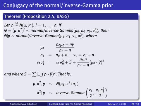
Conjugacy of the normal/inverse-Gamma prior

Theorem (Proposition 2.5, BASS)

Let yiiid∼ N(l, r2), i = 1, . . . , n. If

h = (l, r2)′ ∼ normal/inverse-Gamma(l0, n0, m0, r20), then

h|y ∼ normal/inverse-Gamma(l1, n1, m1, r21), where

l1 =n0l0 + ny

n0 + nn1 = n0 + n, m1 = m0 + n

m1r21 = m0 r2

0 + S +n0 n

n0 + n(l0 - y)2

and where S =∑n

i=1(yi - y)2. That is,

l| r2, y ∼ N(l1, r2/n1)

r2| y ∼ inverse-Gamma(

m1

2,

m1 r21

2

)Simon Jackman (Stanford) Bayesian Inference for Simple Problems February 11, 2012 22 / 30

Marginal Posterior Density, Normal Mean, Conjugacy

The conditional posterior density for l, p(l|y, r2) is a normal densityin which r2 appears in the expression for the variance of theconditional posterior density.

But if we’re interested in l, we want its marginal posterior densityp(l|y)We ‘‘integrate out’’ or ‘‘average over’’ uncertainty with respect to r2;i.e.,

p(l|y) =∫

L

0p(l|r2, y)p(r2|y)dr2

where the limits of integration follow from the fact that variances arestrictly positive.

Resulting marginal density for l is a student-t density.


Marginal Posterior Density, Normal Mean, Conjugacy

Theorem (Proposition 2.6, BASS)Assume conditions of the previous theorem. Then the marginal posteriordensity of l is a student-t density (Definition B.37), with location

parameter l1, scale parameter√

r21/n1 and m1 degrees of freedom, where

n1 = n0 + n,

l1 =n0l0 + ny

n1,

r21 = S1/m1, S1 = m0 r2

0 + (n - 1)s2 + n0 nn1

(y - l0)2, m1 = m0 + n,

s2 =∑n

i=1(yi - y)2 and y = n-1∑ni=1 yi.

Proof.Proposition C.7, BASS.


Posterior Predictive Density, normal data, conjugacy

Consider making a prediction for a future observation, y*.

This quantity also has a posterior density, called a posteriorpredictive density:

p(y*|y) =

∫R+

∫R

p(y*|l, r2, y)p(l, r2|y)dldr2

=

∫R+

∫R

p(y*|l, r2, y)p(l|r2, y)p(r2|y)dldr2

The prediction should not simply condition on particular values ofthe parameters l and r2; we’re uncertain about the predictionbecause we’re uncertain about the parameters l and r2.

The double integral might look a little formidable, but the posteriorpredictive density has a familiar form...


Posterior Predictive Density, normal data, conjugacy

Theorem (Proposition 2.7, BASS)

Let yiiid∼ N(l, r2), (l, r2) ∼ normal/inverse-Gamma(l0, n0, m0, r2

0). Thenthe posterior predictive density for a future observation y*, p(y*|y), is astudent-t density, with location parameter

E(y*|y) = E(l|y) = l1 =n0l0 + ny

n0 + n,

scale parameter r1√

(n1 + 1)/n1 and m1 = n + m0 degrees of freedom,where n1 = n0 + n, r2

1 = S1/m1 and S1 = m0 r20 + (n - 1)s2 + n0 n

n0+n(l0 - y)2.

Proof.Proposition C.8, BASS.


Example 2.13, Suspected voter fraud in Pennsylvania

µ

σ2●

−10 −5 0 5 10

050

100

150

200

µ0 = 0, n0 = 5, ν0 = 6.2, σ02 = 47.07

µ

σ2

●

−10 −5 0 5 10

050

100

150

200

µ1 = −4.69, n1 = 26, ν1 = 27.2, σ12 = 58.44

0 50 100 150 200

0.00

00.

010

0.02

0

σ2

dens

ity

ν0 = 6.2, σ02 = 47.07

0 50 100 150 200

0.00

00.

010

0.02

0

σ2

dens

ity

ν1 = 27.2, σ12 = 58.44

Prior and Posterior normal/inverse-Gamma Densities. Prior densities on the left; posterior densities on the right.Normal/inverse-Gamma densities for (l, r2) in the upper panels, with darker colors indicating regions of higher density, the circleindicating the mode, and for the posterior density, the square indicating the location of the maximum likelihood estimates. Marginalinverse-Gamma densities for r2 appear in the lower panels, with the shaded area corresponding to a 95% highest density region.


Regression

Theorem (Conjugate Prior Normal Regression Model)

yi|xiiid∼ N(xib, r

2)

b|r2 ∼ N(b0, r2B0)

r2 ∼ inverse-Gamma(m0/2, m0r20/2)

then

b|r2, y,X ∼ N(b1, r2B1),

r2|y,X ∼ inverse-Gamma(m1/2, m1 r21/2)

b1 = (B-10 + X′X)-1(B-1

0 b0 + X′Xb)

B1 = (B-10 + X′X)-1

m1 = m0 + n andm1r2

1 = m0r20 + S + r.


Limitations of Conjugacy

seemingly small set of problems amenable to conjugate Bayesiananalysis

e.g., no logit/probit regression!

prior to MCMC revolution, Bayesian ideas interesting, perhaps even‘‘right’’, but extremely difficult (impossible) to implement outsidesmall set of problems

MCMC changed this, circa 1990. Avalanche of Bayesian applicationsin statistics, econometrics. Now standard.

Bayes Theorem to 1990: a long time!

still make use of conjugacy (or conditional conjugacy) inimplementing a MCMC algorithm known as the Gibbs sampler.


bayesian inference for simple problems

Documents