PSYCHOMETRIKA2013DOI: 10.1007/S11336-013-9374-9

BAYESIAN ESTIMATION OF MULTINOMIAL PROCESSING TREE MODELSWITH HETEROGENEITY IN PARTICIPANTS AND ITEMS

DORA MATZKE AND CONOR V. DOLAN

UNIVERSITY OF AMSTERDAM

WILLIAM H. BATCHELDER

UNIVERSITY OF CALIFORNIA, IRVINE

ERIC-JAN WAGENMAKERS

UNIVERSITY OF AMSTERDAM

Multinomial processing tree (MPT) models are theoretically motivated stochastic models for theanalysis of categorical data. Here we focus on a crossed-random effects extension of the Bayesian latent-trait pair-clustering MPT model. Our approach assumes that participant and item effects combine addi-tively on the probit scale and postulates (multivariate) normal distributions for the random effects. Weprovide a WinBUGS implementation of the crossed-random effects pair-clustering model and an applica-tion to novel experimental data. The present approach may be adapted to handle other MPT models.

Key words: multinomial processing tree model, parameter heterogeneity, crossed-random effects model,hierarchical Bayesian modeling.

Multinomial processing tree (MPT) models are theoretically motivated stochastic modelsfor the analysis of categorical data. MPT models can be used to measure the contribution ofthe different cognitive processes that determine performance in various experimental paradigms.Due to their simplicity, MPT models have become increasingly popular over the last decades andhave been applied to a variety of areas in cognitive psychology (for reviews, see Batchelder &Riefer, 1999; Erdfelder, Auer, Hilbig, Aßfalg, Moshagen, & Nadarevic, 2009).

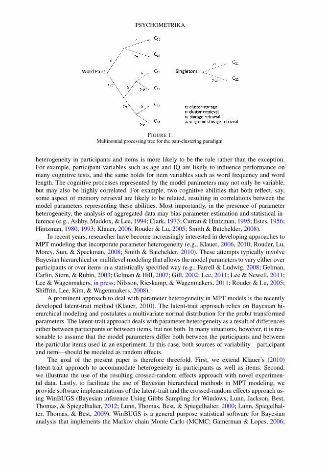
MPT models assume that the observed category responses follow a multinomial distribution.MPT models reparametrize the category probabilities of the multinomial distribution in terms ofa number of model parameters that are assumed to represent underlying cognitive processes. Thecategory probabilities are generally expressed as nonlinear functions of the underlying modelparameters. Specifically, MPT models assume that the observed response categories result fromone or more hypothesized sequences of cognitive events, a structure that can be representedby a rooted tree architecture such as the one depicted in Figure 1. The formal properties of MPTmodels are described by Hu and Batchelder (1994), Purdy and Batchelder (2009), and Riefer andBatchelder (1988). For computer software for fitting and testing MPT models, see for instanceHu and Phillips (1999), Moshagen (2010), and Wickelmaier (2011).

Traditionally, statistical inference for MPT models is carried out on data that are aggre-gated across participants and items using the classical maximum-likelihood approach (e.g., Hu& Batchelder, 1994). This approach relies on the assumption of homogeneity in participants anditems, that is, the assumption that participants and items do not differ substantively in termsof the cognitive processes or characteristics represented by the model parameters. However,

Requests for reprints should be sent to Dora Matzke, Department of Psychology, University of Amsterdam,Weesperplein 4, 1018 XA, Amsterdam, The Netherlands. E-mail: d.matzke@uva.nl

© 2013 The Psychometric Society

PSYCHOMETRIKA

FIGURE 1.Multinomial processing tree for the pair-clustering paradigm.

heterogeneity in participants and items is more likely to be the rule rather than the exception.For example, participant variables such as age and IQ are likely to influence performance onmany cognitive tests, and the same holds for item variables such as word frequency and wordlength. The cognitive processes represented by the model parameters may not only be variable,but may also be highly correlated. For example, two cognitive abilities that both reflect, say,some aspect of memory retrieval are likely to be related, resulting in correlations between themodel parameters representing these abilities. Most importantly, in the presence of parameterheterogeneity, the analysis of aggregated data may bias parameter estimation and statistical in-ference (e.g., Ashby, Maddox, & Lee, 1994; Clark, 1973; Curran & Hintzman, 1995; Estes, 1956;Hintzman, 1980, 1993; Klauer, 2006; Rouder & Lu, 2005; Smith & Batchelder, 2008).

In recent years, researcher have become increasingly interested in developing approaches toMPT modeling that incorporate parameter heterogeneity (e.g., Klauer, 2006, 2010; Rouder, Lu,Morey, Sun, & Speckman, 2008; Smith & Batchelder, 2010). These attempts typically involveBayesian hierarchical or multilevel modeling that allows the model parameters to vary either overparticipants or over items in a statistically specified way (e.g., Farrell & Ludwig, 2008; Gelman,Carlin, Stern, & Rubin, 2003; Gelman & Hill, 2007; Gill, 2002; Lee, 2011; Lee & Newell, 2011;Lee & Wagenmakers, in press; Nilsson, Rieskamp, & Wagenmakers, 2011; Rouder & Lu, 2005;Shiffrin, Lee, Kim, & Wagenmakers, 2008).

A prominent approach to deal with parameter heterogeneity in MPT models is the recentlydeveloped latent-trait method (Klauer, 2010). The latent-trait approach relies on Bayesian hi-erarchical modeling and postulates a multivariate normal distribution for the probit transformedparameters. The latent-trait approach deals with parameter heterogeneity as a result of differenceseither between participants or between items, but not both. In many situations, however, it is rea-sonable to assume that the model parameters differ both between the participants and betweenthe particular items used in an experiment. In this case, both sources of variability—participantand item—should be modeled as random effects.

The goal of the present paper is therefore threefold. First, we extend Klauer’s (2010)latent-trait approach to accommodate heterogeneity in participants as well as items. Second,we illustrate the use of the resulting crossed-random effects approach with novel experimen-tal data. Lastly, to facilitate the use of Bayesian hierarchical methods in MPT modeling, weprovide software implementations of the latent-trait and the crossed-random effects approach us-ing WinBUGS (Bayesian inference Using Gibbs Sampling for Windows; Lunn, Jackson, Best,Thomas, & Spiegelhalter, 2012; Lunn, Thomas, Best, & Spiegelhalter, 2000; Lunn, Spiegelhal-ter, Thomas, & Best, 2009). WinBUGS is a general purpose statistical software for Bayesiananalysis that implements the Markov chain Monte Carlo (MCMC; Gamerman & Lopes, 2006;

DORA MATZKE ET AL.

Gilks, Richardson, & Spiegelhalter, 1996) algorithm necessary for Bayesian parameter estima-tion (for an introduction for psychologists, see Kruschke, 2010; Lee & Wagenmakers, in press;Sheu & O’Curry, 1998). We will use the pair-clustering model—one of the most extensivelystudied MPT models—as an example. However, the crossed-random effects approach presentedhere may in principle be adapted to handle many other MPT models as well.

The paper is organized as follows. The first section introduces various methods to accommo-date parameter heterogeneity in MPT models. The second section introduces the pair-clusteringMPT model in more detail. The third section presents the WinBUGS implementation of thelatent-trait pair-clustering model. The fourth section presents the crossed-random effects pair-clustering model with the corresponding WinBUGS implementation and describes the results ofapplying the model to novel experimental data. The fifth section concludes the paper.

1. Parameter Heterogeneity in MPT Models

The data for an MPT model consist of category responses from several participants to eachof a set of items. MPT model parameters, θp , p = 1, . . . ,P , represent probabilities of latentcognitive capacities, such as attending to an item, storing an item in memory, retrieving an itemfrom memory, detecting the source of an item, making an inference, or guessing a response. Suchparameters are functionally independent and each has parameter space [0,1].

Parameter estimation and statistical inference for MPT models is traditionally carried outon response category frequencies aggregated over participants and items using maximum like-lihood methods (e.g., Hu & Batchelder, 1994). This approach is based on the assumption ofparameter homogeneity. If this assumption is violated, the analysis of aggregated data may leadto erroneous conclusions. The consequences of variability are especially troubling for nonlin-ear models, such as MPT models. In particular, reliance on aggregated data in the presence ofparameter heterogeneity may lead to biased parameter estimates, the underestimation of con-fidence intervals, and the inflation of Type I error rates (e.g., Batchelder, 1975; Batchelder &Riefer, 1999; Heathcote, Brown, & Mewhort, 2000; Klauer, 2006; Riefer & Batchelder, 1991;Rouder & Lu, 2005). Moreover, the specific pattern of the parameter correlations can greatly in-fluence the magnitude of the deleterious effects of unmodeled parameter heterogeneity (Klauer,2006).

In recent years, a growing number of researchers has started to use cognitive models thataccommodate heterogeneity in participants and/or items (e.g., DeCarlo, 2002; Karabatsos &Batchelder, 2003; Lee, 2011; Lee & Webb, 2005; Navarro, Griffiths, Steyvers, & Lee, 2006;Rouder & Lu, 2005; Rouder, Sun, Speckman, Lu, & Zhou, 2003; Rouder, Lu, Sun, Speckman,Morey, & Naveh-Benjamin, 2007). In the context of MPT models, Klauer (2006) and Smith andBatchelder (2008) proposed statistical tests for detecting parameter heterogeneity. Moreover, anumber of approaches that deal with parameter heterogeneity are now available for MPT models.

These approaches rely on hierarchical modeling and postulate population-level (hyper)distributions for the model parameters. The population-level distributions describe the vari-ability in parameters either across participants or across items (e.g., Gelman et al., 2003;Gelman & Hill, 2007; Gill, 2002). For instance, Klauer (2006; see also Stahl & Klauer, 2007) pro-posed the use of latent-class MPT models with discrete population-level distributions to modelthe between-participant variability and the correlations between the model parameters. In con-trast, Smith and Batchelder (2010) proposed to capture the between-participant variability ofthe model parameters using independent beta distributions (see also Batchelder & Riefer, 2007;Karabatsos & Batchelder, 2003; Riefer & Batchelder, 1991).

Here we will focus on yet another alternative—the latent-trait approach—which assumesa multivariate normal distribution for the participant differences in the probit transformed pa-rameters and accounts for the correlations between the model parameters (Klauer, 2010). The

PSYCHOMETRIKA

latent-trait approach relies on Bayesian parameter estimation, but the MCMC algorithm for esti-mating the model parameters is currently not implemented in any off-the-shelf software package.

All the above described alternatives deal with parameter heterogeneity as a result of dif-ferences either between participants or between items, but not both, and rely on data that areaggregated either over items or over participants. It is, however, often reasonable to assume thatthe model parameters vary between participants as well as between items. In such situations,participant and item differences should be modeled as crossed-random effects (Clark, 1973) andinference should be based on participant-by-item data.

In psychometrics, there is a long tradition of simultaneously modeling variability in par-ticipants and items (e.g., De Boeck, 2008; Lord & Novick, 1986). In cognitive psychology, incontrast, such modeling constitutes a relatively recent trend (e.g., Baayen, 2008). For instance,Rouder et al. (2007) and Rouder and Lu (2005) have recently developed hierarchical signal de-tection models that incorporate random participant and item effects. In MPT modeling, attemptsto simultaneously model heterogeneity in participants and items are scarce.

Augmenting MPT models with participant and item variability requires a separate parameterfor each participant-item combination, θijp , where i = 1, . . . , I indexes the participants, j =1, . . . , J indexes the items, and p = 1, . . . ,P indexes the model parameters in θ = (θijp). Thisrequirement leads to I × J × P parameters for only I × J data points, resulting in problemswith model identification. We can reduce the number of parameters by using, for example, areparametrization of the two-parameter Rasch model (e.g., Fischer & Molenaar, 1995). We canthen model each participant-item combination using

θijp = αipβjp

αipβjp + (1 − αip)(1 − βjp), (1)

for αip,βjp ∈ (0,1) (Batchelder, 1998, 2009). Here αip and βjp denote the ith participant ef-fect and the j th item effect relating to parameter p, respectively. Karabatsos and Batchelder(2003) developed this Rasch model approach for the General Condorcet MPT Model. Batchelderand Browther (1997) also used a Rasch model decomposition and modeled the logit trans-formed participant-item parameters as additive functions of the participant and item effects. SeeDe Boeck and Partchev (2012) for an alternative approach to model heterogeneity in participantsand items in MPT models using item response theory.

In the present paper we will explore an alternative that extends Klauer’s (2010) latent-traitapproach to simultaneously deal with heterogeneity in participants and items. Specifically, wewill model the probit transformed θijp parameters as additive combinations of participant anditem effects. The participant and item effects are then assumed to come from (multivariate) nor-mal distributions. Rouder et al. (2008) used a similar approach for a simple hierarchical processdissociation model, where they assumed the additivity of the probit transformed participant anditem effects and modeled these using multivariate normal priors (see also Rouder & Lu, 2005;Rouder et al., 2007).

To summarize, a number of hierarchical approaches are now available for MPT models todeal with heterogeneity introduced either by the participants or by the items. The latest amongthese methods, Klauer’s (2010) latent-trait approach, assumes a multivariate normal distributionfor the probit transformed parameters and incorporates the possibility of parameter correlations.The latent-trait approach deals with parameter heterogeneity as a result of differences either be-tween participants or between items, but not for both sources. The latent-trait approach mayreadily be augmented to accommodate crossed-random effects by assuming additivity of partic-ipant and item effects on the probit scale.

DORA MATZKE ET AL.

2. The Pair-Clustering MPT Model

The pair-clustering model—one of the most extensively studied MPT models—was devel-oped for the measurement of the storage and retrieval processes that underlie performance in thepair-clustering paradigm (e.g., Batchelder & Riefer, 1980, 1986). The pair-clustering paradigminvolves a free recall memory experiment, where participants study a list of words that consistsof two types of items: semantically related word pairs (e.g., dog–cat, father–son) and single-tons (i.e., unpaired words, such as paper and train). Participants are presented with the studylist in a word-by-word fashion, such as dog–paper–father–train–cat–son–etc. After the presen-tation of the study list, participants are required to recall, in any order, as many words as theycan. The general finding is that semantically related word pairs are recalled consecutively, as a‘pair-cluster’.

Since its development, the pair-clustering model has facilitated the interpretation of numer-ous free recall phenomena, such as retroactive inhibition and the effects of presentation rate andstimulus spacing (see Batchelder & Riefer, 1999). Moreover, the pair-clustering model has beenused successfully to investigate memory deficits in various age groups and clinical populations(e.g., Bröder, Herwig, Teipel, & Fast, 2008; Golz & Erdfelder, 2004; Riefer & Batchelder, 1991;Riefer, Knapp, Batchelder, Bamber, & Manifold, 2002; see Batchelder & Riefer, 2007 for a re-view).

The architecture of the pair-clustering model can be represented by a rooted tree structureshown in Figure 1. The responses of each participant fall into two independent category systems,namely responses to word pairs and responses to singletons. Each category system k = 1,2 ismodeled by a separate subtree of the multinomial model, where each subtree consists of a finitenumber of branches terminating in one of the response categories Ckl , l = 1, . . . ,Lk . The recallof word pairs is scored into four response categories (L1 = 4): C11, both members of a word pairare recalled consecutively; C12, both members of a word pair are recalled but not consecutively;C13, only one member of a word pair is recalled; and C14, neither member of a word pair isrecalled. The recall of singletons is scored in two response categories (L2 = 2): C21, singleton isrecalled; and C22, singleton is not recalled.

The pair-clustering model explains the observed data by reparametrizing the category prob-abilities, Pr(Ckl), of the multinomial distribution in terms of p = 1, . . . ,4 functionally indepen-dent model parameters θ = (c, r, u, a), with θp ∈ (0,1). Parameter c represents the probabilitythat a word pair is clustered and stored in memory. Parameter r is the conditional probability thata word pair is retrieved from memory, given that it was clustered. Parameter u is the conditionalprobability that a member of a word pair is stored and retrieved from memory, given that theword pair was not stored as a cluster. As the u parameter taps both the storage and retrieval ofunclustered words, it is typically regarded as a nuisance parameter. Parameter a is the probabilitythat a singleton is stored and retrieved from memory. As illustrated later, it is frequently assumedthat a = u, i.e., the probability that a singleton is stored and retrieved (a) equals the probabilitythat a member of a word pair is stored and retrieved, given that it was not clustered (u). The pair-clustering model has four free response categories and it features at most four model parameters.The identification of the pair-clustering model has been established elsewhere (e.g., Batchelder& Riefer, 1986).

According to the model, if a word pair is successfully clustered and retrieved with jointprobability cr , the two members of the word pair are retrieved consecutively, resulting in recallcategory C11. If a word pair is successfully clustered (c) but is not retrieved (1-r), neither mem-ber of the word pair is retrieved, resulting in recall category C14. The model thus assumes thatclustered pairs are either retrieved as a pair or are not retrieved at all. In contrast, if word pairsare not clustered (1-c), either member of the word pair can be stored and retrieved independentlywith probability u, resulting in recall category C12 or C13. Retrieved items from unclusteredword pairs are thus not recalled consecutively.

PSYCHOMETRIKA

The probabilities of the six response categories are expressed in terms of the model param-eters as follows:

Pr(C11|θ) = cr

Pr(C12|θ) = (1 − c)u2

Pr(C13|θ) = (1 − c)2u(1 − u)

Pr(C14|θ) = c(1 − r) + (1 − c)(1 − u)2

Pr(C21|θ) = a

Pr(C22|θ) = 1 − a.

(2)

The raw data in category system k consist of the response of a given participant i = 1, . . . , I

to a particular item j = 1, . . . , Jk , represented by a vector of length Lk . For a given participant-word pair combination, the raw data nij,1 thus consist of a vector of length L1 = 4, where theentry nijl equals 1 if the response of participant i to word pair j falls into response category l,and zero otherwise. For example, if participant i recalls both members of word pair j consecu-tively (i.e., response category C11), the raw data are given by the vector (1,0,0,0). Similarly, fora given participant-singleton combination, the raw data nij,2 consist of a vector of length L2 = 2,where nijl equals 1 if the response of participant i to singleton j falls into response category l,and zero otherwise. For example, if participant i does not recall singleton j (i.e., response cate-gory C22), the raw data are given by the vector (0,1). Traditional analysis of pair-clustering dataassumes that observations over participant and items are independent and identically distributed.Parameter estimation is generally carried out on category responses summed over participantsand items (e.g., Batchelder & Riefer, 1986).

3. The Latent-Trait Pair-Clustering Model

The main goal of the present paper is to augment Klauer’s (2010) Bayesian latent-trait ap-proach to handle heterogeneity in both participants and items. To facilitate this, we first introducethe latent-trait approach in more detail and provide a WinBUGS implementation of the latent-traitpair-clustering model. We then report the results of a parameter recovery study. In what followswe assume that the items are homogeneous and use the latent-trait approach to model individualdifferences between participants. Note, however, that the latent-trait approach may just as wellbe used to capture the variability between items instead of participants. In this case, we wouldassume that participants are homogeneous and model the differences between the items.

3.1. Introduction to the Latent-Trait Approach

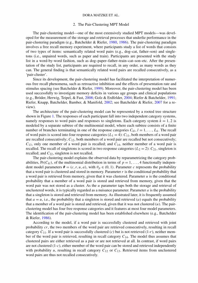
The symbols and notation used in the text, figures, and the WinBUGS scripts are summarizedin Table 1. As we focus on parameter heterogeneity as a result of individual differences betweenparticipants, the raw data are aggregated over the J1 word pairs and the J2 singletons but not overthe i = 1, . . . , I participants. The data of participant i consist thus of the frequency of responses,nikl , falling into recall category Ckl , k = 1,2, l = 1, . . . ,Lk .

For each participant i in each category system k, the observed category frequencies areassumed to follow a multinomial distribution with category probabilities Pr(Ckl |θ i ). Formally,let Bklm be the mth branch terminating in Ckl , m = 1, . . . ,Mkl . The probability that participant i

DORA MATZKE ET AL.

TABLE 1.Notation.

Notation Explanation

K Number of category systemsLk Number of response categories in category system k

I Number of participantsJk Number of items in category system k

Pk Number of parameters in category system k

Ckl Response category l in category system k

Mkl Number of branches terminating in Ckl

Bklm mth branch terminating in Ckl

nij,kl Response (i.e., 0 or 1) of participant-item combination ij in Ckl

θijpkParameter p of participant-item combination ij in category system k (i.e., c, r , u for k = 1;a for k = 2)

vkl,mp Number of nodes on Bklm associated with θpk

wkl,mp Number of nodes on Bklm associated with 1 − θpk

θprtijpk

Probit transformed parameter p of participant-item combination ij in category system k

μpk Group mean for parameter θprtpk

μμpkMean of normal prior for μpk

σμpkStandard deviation of normal prior for μpk

δrawpartipk

ith unscaled participant effect relating to parameter pk

ξpartpkScaling factor for the participant effects relating to parameter pk

δpartipkith scaled participant effect relating to parameter pk

Tpart Unscaled variance–covariance matrix of participant effectsSpart Scaled variance–covariance matrix of participant effectsσpartpk

Scaled standard deviation of participant effects relating to parameter pk

ρpartpkp′k

Correlation between participant effects relating to parameter pk and p′k

δrawitemjpk

j th unscaled item effect relating parameter pk

ξitempkScaling factor for the item effects relating to parameter pk

δitemjpkj th scaled item effect relating to parameter pk

Titem Unscaled variance–covariance matrix of item effectsa

Sitem Scaled variance–covariance matrix of item effectsa

λitempkUnscaled standard deviation of item effects relating to parameter pk

b

σitempkScaled standard deviation of item effects relating to parameter pk

ρitempkp′k

Correlation between item effects relating to parameter pk and p′k

a

Note. For the latent-trait approach, the k subscript of the parameter index p is suppressed throughout thetext because ui = ai . The aindicates item parameters that are used only for the real data example featuringcorrelated item effects. The bindicates item parameters that are used only for the parameter recovery studyfeaturing uncorrelated item effects.

follows branch Bklm is given by

Pr(Bklm|θ i ) =P∏

p=1

θvklmp

ip (1 − θ)wklmp

ip , (3)

where vklmp ≥ 0 and wklmp ≥ 0 are the number of nodes on branch Bklm that is associated withparameter θp , p = 1, . . . ,P , and 1 − θp , respectively. The probability of each response category

PSYCHOMETRIKA

is given by adding the probabilities of all the branches that lead to that category:

Pr(Ckl |θ i ) =Mkl∑

m=1

P∏

p=1

θvklmp

ip (1 − θip)wklmp . (4)

The data of participant i across the two category systems, ni = (ni1,ni2), are assumed to followa multinomial distribution:

Pr(Ni = ni |θ i ) =K∏

k=1

{Jk!

nik1! × nik2! × · · · × nikLk!

Lk∏

l=1

[Pr(Ckl |θ i )

]nikl

}. (5)

The latent-trait approach relies on Bayesian hierarchical modeling that allows the individualmodel parameters θip to vary over participants in a statistically specified way. The method pos-tulates a multivariate normal distribution to capture the between-participant variability and thecorrelations between the model parameters. The latent-trait approach relies on MCMC samplingto approximate the posterior distributions of the model parameters. In what follows, we presentan easy-to-use WinBUGS implementation of the latent-trait approach that enables researchers toobtain samples from the posterior distribution of the model parameters.

3.2. WinBUGS Implementation of the Latent-Trait Pair-Clustering Model

The graphical model for the WinBUGS implementation of the latent-trait pair-clusteringmodel is shown in Figure 2. Observed variables are represented by shaded nodes and unob-served variables are represented by unshaded nodes. Continuous variables are represented bycircles and discrete variables are represented by squares. The graph structure indicates depen-dencies between the nodes and the plates represent independent replications (e.g., Lee, 2008).The graphical model depicts the basic pair-clustering model for I participants responding toJ1 word pairs and J2 singletons, with the constraint that a = u. The corresponding WinBUGSscript is available as supplemental material at http://dora.erbe-matzke.com/publications.html andhttps://www.dropbox.com/sh/stgt80dkegskdfk/3KvGGJ6Th7/MPT_OnlineAppendix.zip.

Data For each participant, the data for word pairs, ni1, follow a multinomial distribu-tion, with category probabilities Pr(C11|θ i ), Pr(C12|θ i ), Pr(C13|θ i ), Pr(C14|θ i ), and J1. Foreach participant, the data for singletons, ni2, follow a multinomial distribution with Pr(C21|θ i ),Pr(C22|θ i ), and J2.

Prior Distributions The basic model depicted in Figure 2 assumes three parameters perparticipant (P = 3): θ i = (ci, ri , ui). Thus, we assume that ai = ui . The individual model param-eters θip are transformed from the probability scale to the real line using a probit link so that thetransformed parameters θ

prtip are given by Φ−1(θip), where Φ is the standard normal cumulative

distribution function. The use of probit transformed probabilities has a long history in psycho-metrics, and is also common practice in Bayesian cognitive modeling (e.g., Rouder & Lu, 2005;Rouder et al., 2007, 2008). To model participant heterogeneity and parameter correlations, weassume that the probit transformed parameters θ

prti follow a multivariate normal distribution with

mean μ and variance–covariance matrix Spart. The θprtip parameters are reparametrized as follows:

θprtip = μp + δpartip , (6)

where μp is the group mean for parameter p and δpartip is the ith participant’s deviation fromit. The δparti parameters are then drawn from a zero-centered multivariate distribution withvariance–covariance matrix Spart.

DORA MATZKE ET AL.

FIGURE 2.Graphical model for the latent-trait pair-clustering model. θi1 = ci , θi2 = ri , and θi3 = ui . Note. To maintain consistencywith the WinBUGS syntax, the multivariate normal and independent normal distributions are parametrized in terms ofthe precision (i.e., inverse variance).

Hyper-Prior Distributions The population-level μ and Spart parameters are estimated fromthe data and therefore require prior distributions. The priors for the μp parameters are indepen-dent normal distributions with μμp = 0 and σ 2

μp= 1. Note that the original formulation of the

latent-trait approach (Klauer, 2010) assumes independent normal distributions with μμp = 0 andσ 2

μp= 100. However, we prefer to use σ 2

μp= 1 because it corresponds to a uniform distribution

on the probability scale (Rouder & Lu, 2005).The prior for the variance–covariance matrix Spart is a scaled Inverse-Wishart distribution.

The Inverse-Wishart is a frequently used prior for variance–covariance matrices (Gelman & Hill,2007). The Inverse-Wishart prior has two parameters: the degrees of freedom that is set to oneplus the number of free participant parameters (1 + P ) and the scale matrix that is set to theP × P identity matrix (W). The advantage of the Inverse-Wishart is that it results in an unin-

PSYCHOMETRIKA

formative uniform prior distribution between −1 and 1 for the ρpp′ correlation parameters. Thedisadvantage is that the Inverse-Wishart with 1 + P degrees of freedom imposes a very restric-tive prior on the standard deviations. To be able to estimate the standard deviations more freely,we augment the Inverse-Wishart with a set of scale parameters, ξpart = [ξpart1 , . . . , ξpartP ] (Gel-man & Hill, 2007). The resulting scaled Inverse-Wishart distribution still implies a uniform priordistribution for the correlation parameters, but it allows the standard deviations to be estimatedmore freely than does the Inverse-Wishart. The variance–covariance matrix Spart is then modeledas

Spart = Diag(ξpart)TpartDiag(ξpart), (7)

where Diag(ξ) is a diagonal matrix containing the scale parameters. Tpart follows an Inverse-Wishart distribution with 1 + 3 degrees of freedom, with a scale matrix that is set to the 3 × 3identity matrix. The standard deviations can be obtained by

σpartp = |ξpartp | ×√

Tpartpp. (8)

The correlation parameters are given by

ρpartpp′ = ξpartpξpartp′ Tpartpp′

|ξpartp |√

Tpartpp× |ξpartp′ |

√Tpartp′p′

. (9)

The ξpartp parameters are given uniform distributions ranging from 0 to 100 (e.g., Gelman& Hill, 2007). Klauer (2010) used normal distributions with a mean of one and a variance of100 as prior for the scaling parameters. In our WinBUGS implementation, these priors occa-sionally resulted in convergence problems for the variance and the correlation parameters. Notethat the use of redundant multiplicative parameters, such as ξpartp , has been reported to increasethe rate of convergence in hierarchical models (Gelman & Hill, 2007). As a result of the newparametrization, Equation (6) can be reformulated as follows:

θprtip = μp + ξpartp × δraw

partip, (10)

where μp is the group mean for parameter p, ξpartp is the scaling factor of the scaled Inverse-Wishart distribution, and δraw

partipis the ith participant’s unscaled deviation from the group mean.

3.3. Parameter Recovery Study

We conducted a series of parameter recovery studies to assess whether the WinBUGS im-plementation of the latent-trait pair-clustering model adequately recovers true parameter values.Here we report the results of a study where we generated free recall data for synthetic partici-pants responding to a set of word pairs and singletons in two sessions of the pair-clustering task.The resulting data sets were fit with the latent-trait pair-clustering model using WinBUGS.

Methods Each synthetic participant performed the pair-clustering task two consecutivetimes. For each participant, the data from the two sessions were scored into four category sys-tems: word pairs and singletons for the first session and word pairs and singletons for the secondsession. We ran three sets of simulations, each comprising 100 data sets. First, each data setcontained observations from 63 (I = 63) synthetic participants, responding to 10 word pairs(J1 = 10) and 5 singletons (J2 = 5) in each of the two sessions. Second, each data set containedobservations from 63 participants, responding to 20 word pairs and 10 singletons in each of thetwo sessions. Third, each data set contained observations from 126 participants, responding to10 word pairs and 5 singletons in each of the two sessions.

DORA MATZKE ET AL.

Similar to Klauer’s (2010) recovery study, we used five parameters (P = 5) per participantacross the two sessions: θ i = (c1i

, ri , u1i, c2i

, u2i). The following parameter constraints were

imposed: r1i= r2i

, a1i= u1i

, and a2i= u2i

. The generating population-level parameter valuesare shown in Figure 3. We conducted several recovery studies using alternative true parametervalues. The results were essentially the same as the ones reported here. Note that the details ofthe recovery study, including the true parameter values and the number of participants and items,are identical to those used in Klauer’s paper.

For each analysis reported in this article, we ran three MCMC chains and used randomlygenerated overdispersed starting values to confirm that the chains have converged to the station-ary distribution. Convergence is confirmed if the individual chains are indistinguishable fromeach other. Convergence was formally assessed with the R̂ statistic (Brooks & Gelman, 1998;Gelman & Rubin, 1992), a quantitative measure of convergence that compares the within-chainvariance to the between-chain variance. The results reported in this article are based on analyseswhere R̂ for all parameters of interest (i.e., group means, random effects, and the standard devi-ation and the correlation of the random effects) is lower than 1.05. In light of the possibility ofhigh autocorrelations between successive MCMC samples, we ran relatively long MCMC chainsand thinned each chain by retaining samples from only every third iteration.

The latent-trait pair-clustering model was fit to the synthetic data sets using WinBUGS. Foreach data set, we discarded the first 2,000 samples of each chain as burn-in and based inferenceon a total of 54,000 recorded samples.

Results The results of the recovery study for the group-level parameters are shown in Fig-ure 3. We follow Klauer’s (2010) practice and use the median and the standard deviation to sum-marize the posterior distribution of the parameters. Also, the posterior median is often preferableover the posterior mode or the posterior mean for non-symmetric or heavy tailed posterior dis-tributions. Note that the group c1, r , u1, c2, and u2 parameters are reported on the probabilityscale, while their standard deviations and correlations are reported on the probit scale. The groupparameters and their standard deviations are recovered relatively well using the posterior medianeven for the first set of simulations with relatively few participants and very few items. Naturally,as the number of items or the number of participants increases, the bias, the posterior standarddeviation, and the standard error of the recovered parameters decrease. The storage-retrieval u1

and u2 parameters and their standard deviations are estimated most precisely, as indicated by thesmall posterior standard deviation of the estimates. The cluster-retrieval r parameter and its stan-dard deviation are estimated the least precisely as evidenced by the greater posterior uncertaintyof the estimates, especially for the first set of simulations.

With respect to the correlation parameters, the results are less clear-cut. Similar to Klauer’s(2010) findings, the posterior median underestimates the parameter correlations especially in datasets with few participants and items. The posterior standard deviations are rather large, indicatinglarge uncertainty in the estimates. Nevertheless, as the number of participants or the number ofitems increases, the bias, the posterior standard deviations and the standard error of the recoveredcorrelations decrease. As for the standard deviations, correlations involving the cluster-retrievalr parameter are the least well estimated, especially for the first set of simulations.

To sum up, the results of the simulation study indicated that the WinBUGS version of thelatent-trait pair-clustering model adequately recovered the true parameter values. In the nextsection, we extend the latent-trait pair-clustering model and the corresponding WinBUGS scriptto handle heterogeneity in both participants and items.

PSYCHOMETRIKA

FIGURE 3.Posterior medians from the parameter recovery study for the latent-trait pair-clustering model using WinBUGS. Each setof simulations consisted of 100 data sets. The black bullets indicate the mean of the posterior median of the parametersacross the 100 replications. The black vertical lines are based on the mean of the posterior standard deviation across the100 replications. The gray vertical lines indicate the standard error of the posterior median across the 100 replications.

4. The Crossed-Random Effects Pair-Clustering Model

In many applications of MPT models, it is reasonable to assume that the model parametersdo not only differ between participants but also between the items used in a particular experi-

DORA MATZKE ET AL.

ment. We should then treat both participant and items effects as random, define parameters foreach participant-item combination and base statistical inference on the unaggregated data. Thissection introduces a crossed-random effects pair-clustering model that is based on an extensionof Klauer’s (2010) latent-trait approach. Our crossed-random effects model assumes that the par-ticipant and item effects combine additively on the probit scale. The participant and item effectsare modeled with multivariate normal and independent normal distributions, respectively, withmeans and (co)variances estimated from the data.

4.1. Introduction to the Crossed-Random Effects Approach

In the crossed-random effects pair-clustering model, statistical inference is based on un-aggregated participant-by-item data. In a given category system k, k = 1,2, the raw categoryresponses of each participant-item combination, i = 1, . . . , I , j = 1, . . . , Jk , are assumed to fol-low a multinomial distribution with category probabilities Pr(Ckl |θ ijk

), l = 1, . . . ,Lk , where θ ijk

contains the p = 1, . . . ,Pk model parameters of participant-item combination ij in category sys-tem k.

The requirement of a separate parameter for each participant-item combination leads to avery large number of parameters, resulting in problems of model identification. To reduce thenumber of parameters, we assume that the probit transformed parameters are given by the addi-tive combination of participant and item effects (e.g., Rouder & Lu, 2005; Rouder et al., 2007,2008). More formally, the crossed-random effects pair-clustering model assumes that the probittransformed participant-item parameters in category system k are given by

θprtijpk

= μpk+ δpartipk

+ δitemjpk, (11)

where μpkis the group mean for parameter p in category system k, and δpartipk

and δitemjpkare

the ith participant effect and the j th item effect, respectively. We postulate a multivariate normaldistribution to describe variability between participants and independent normal distributions tocapture the variability between items. The participant effects are thus allowed to be correlated apriori, whereas the item effect are not. Naturally, we may model the correlations between the itemeffects—similar to the participant effects—using a multivariate normal distribution. The possibil-ity to incorporate correlated participant and correlated item effects will be demonstrated shortlyusing experimental data. The next section presents an easy-to-use WinBUGS implementation ofthe crossed-random effects pair-clustering model.

4.2. WinBUGS Implementation of the Crossed-Random Effects Pair-Clustering Model

The graphical model for the WinBUGS implementation of the crossed-random effect pair-clustering model is shown in Figure 4. The graphical model depicts the basic pair-clusteringmodel for I participants responding to J1 word pairs and J2 singletons. The corresponding Win-BUGS script is available as supplemental material.

4.2.1. Data The raw data of each participant-word pair combination, nij,1, follow amultinomial distribution, with category probabilities Pr(C11|θ ij1), Pr(C12|θ ij1), Pr(C13|θ ij1),Pr(C14|θ ij1). Similarly, the raw data for each participant-singleton combination, nij,2, followa multinomial distribution, with category probabilities Pr(C21|θ ij2), Pr(C22|θ ij2).

4.2.2. Prior Distributions The crossed-random effects pair-clustering model posits a sep-arate parameter for each participant-item combination in each category system k. These θijpk

parameters are transformed from the probability scale to the real line using the probit link. Asgiven in Equation (11), the probit transformed parameters θ

prtijpk

are given by the additive combi-nation of participant and item effects.

PSYCHOMETRIKA

FIGURE 4.Graphical model for the crossed-random effects pair-clustering model. θij1 = cij , θij2 = rij , θij3 = uij . Note. Tomaintain consistency with the WinBUGS syntax, the multivariate normal and independent normal distributions areparametrized in terms of the precision (i.e., inverse variance).

DORA MATZKE ET AL.

In the category system for word pairs, the model assumes three participant effects for eachparticipant (i.e., δpartic , δpartir , and δpartiu ) and three item effects for each word pair (i.e., δitemjc

,δitemjr

, and δitemju). The model postulates thus three parameters for each participant-word pair

combination (P1 = 3): θ ij1 = (cij , rij , uij ). For singletons, the model assumes one participanteffect per participant (δpartia ) and one item effect per singleton (δitemja

). The model postulatesthus one parameter for each participant-singleton combination (P2 = 1) : θij2 = aij .

In the basic pair-clustering model depicted in Figure 4, the constraint that a = u may beimplemented as follows. First, the group mean of the singleton storage-retrieval a parameter isconstrained to be equal to the group mean of the storage-retrieval u parameter: μa = μu. Second,note that the basic model assumes that each participant is presented with J1 word pairs and J2singletons. We are thus able to place across-category system constraints on the participant effects,because responses from a given participant are available in both category systems: δpartia = δpartiu .Third, we are unable to place across-category system constraints on the items effects because agiven item appears in only one of the category systems: responses to each of the J1 word pairs areonly available in the first category system, whereas responses to each of the J2 singletons are onlyavailable in the second category system. Nevertheless, we may assume that the standard deviationof the item effects relating to a and u are equal: σitema = σitemu . A possibility for across-categorysystem constraints on the item effects will be illustrated shortly using experimental data.

The δparti parameters are assumed to come from a zero-centered multivariate normal distri-bution, with variance–covariance matrix Spart estimated from the data. The δitemjpk

parametersare drawn from zero-centered independent normal distributions, with the standards deviationsσitempk

estimated from the data.

4.2.3. Hyper-Prior Distributions The priors for the grand mean μpkparameters are

weakly informative independent normal distributions with μμpk= 0 and σ 2

μpk= 1. The prior

for Spart is a scaled Inverse-Wishart distribution. The degrees of freedom of the scaled Inverse-Wishart equals one plus the number of free participant effects. In the model shown in Figure 4,we postulate three participant effects across the two category systems, resulting in four degreesof freedom. The scale matrix is set to the 3 × 3 identity matrix (W). The scaling factor ξpartparameters of the Inverse-Wishart are given uniform distributions ranging from 0 to 100. Thestandard deviations and the correlations of the participant effects can be obtained using Equa-tion (8) and (9), respectively.

The priors for the σ 2itempk

variance parameters are independent scaled inverse gamma distri-

butions with α = 1 and β = 1. The inverse gamma distribution with α and β set to low values,such as 1, 0.01, or 0.001 is a frequently used prior for variance parameters (e.g., Spiegelhalter,Thomas, Best, Gilks, & Lunn, 2003). In order to increase the rate of convergence, we augmenteach variance parameter with a redundant multiplicative scaling parameter ξitem, a techniquecalled parameter expansion (Gelman & Hill, 2007). In the expanded model, the item standarddeviations are given by

σitempk= |ξitempk

| × λitempk, (12)

where ξitempkis the scaling factor and λitempk

is the unscaled item standard deviation for param-eter p in category system k. The ξitem parameters are given uniform distributions ranging from0 to 100. As a result of expanding the model with the ξpart and ξitem parameters, Equation (11),can be reformulated as follows:

θprtijpk

= μpk+ ξpartpk

× δrawpartipk

+ ξitempk× δraw

itemjpk, (13)

where δrawpartipk

and δrawitemjpk

are the unscaled effects for participant i and item j relating to param-

eter p in category system k, respectively.

PSYCHOMETRIKA

4.3. Parameter Recovery Study

We conducted a series of parameter recovery studies to examine whether the crossed-randomeffects pair-clustering model adequately recovers true parameter values. Here we report the re-sults of a study where we generated free recall data for synthetic participants responding to thesame set of word pairs and the same set of singletons in two sessions of the pair-clustering task.We analyzed the resulting data sets with the crossed-random effects pair-clustering model usingWinBUGS.

Methods Each synthetic participant performed the pair-clustering task two consecutivetimes using the same set of word pairs and the same set of singletons. For each participant-word pair combination, the data from the two sessions were scored into two separate categorysystems. Similarly, for each participant-singleton combination, the data from the two sessionswere scored into two separate category systems. We conducted three sets of simulations, eachcomprising 100 synthetic data sets. First, each data set contained observations from 63 (I = 63)synthetic participants, responding to the same set of 10 word pairs (J1 = 10) and the same setof 5 singletons (J2 = 5) in each of the two sessions. Second, each data set contained observa-tions from 63 participants, responding to 20 word pairs and 10 singletons in each of the twosessions. Third, each data set contained observations from 126 participants, responding to 10word pairs and 5 singletons in each of the two sessions. We used five (P1 = 5) parameters foreach participant-word pair combination: θ ij1 = (c1,ij , rij , u1,ij , c2,ij , u2,ij ). The cluster-retrievalr parameter was thus constrained to be equal across the two sessions, r1,ij = r2,ij = rij . We usedtwo (P2 = 2) parameters for each participant-singleton combination: θ ij2 = (a1,ij , a2,ij ).

As the same set of word pairs and singletons were used across the two sessions, the J1 itemseffects relating to c, r , and u, and the J2 item effects relating to a were assumed to be equalacross the two sessions. We followed the approach described earlier to implement the constraintthat a = u. The generating parameter values for the population-level parameters are shown inFigure 5.

The crossed-random effects pair-clustering model was fit to the synthetic data sets usingWinBUGS. As before, we monitored samples from every third iteration, we discarded the first2,000 samples of each chain as burn-in, and based inference on a total of 54,000 recorded sam-ples.

Results The results of the recovery study for the group-level model parameters are shownin Figure 5. As before, the group c1, r , u1, c2, and u2 parameters are reported on the probabilityscale, while the standard deviations and the correlations are reported on the probit scale. Thegroup parameters and the participant and item effect standard deviations are approximated wellusing the posterior median even for the first set of simulations with relatively few participantsand very few items. Again, the storage-retrieval u1 and u2 parameters and the correspondingstandard deviations are estimated most precisely and the cluster-retrieval r parameter and thecorresponding standard deviations are estimated least precisely. As the number of items or thenumber of participants increases, the bias, the posterior standard deviation, and the standard errorof the recovered parameters decrease.

With respect to the participant effect correlations, the results are again less straightforward.The posterior median underestimates the parameter correlations, especially in the first set ofsimulations with relatively few participants and very few items. The posterior standard deviationsare quite large, suggesting large uncertainty in the estimates. Naturally, increasing the number ofparticipants or the number of items decreases the bias, the posterior standard deviation, and thestandard error of the recovered correlations. Again, correlations involving the cluster-retrieval r

parameter are the least well estimated.

DORA MATZKE ET AL.

FIGURE 5.Posterior medians from the parameter recovery study for the crossed-random effects pair-clustering model using Win-BUGS. Each set of simulations consisted of 100 data sets. The black bullets indicate the mean of the posterior medianof the parameters across the 100 replications. The black vertical lines are based on the mean of the posterior standarddeviation across the 100 replications. The gray vertical lines indicate standard error of the posterior median across the100 replications.

PSYCHOMETRIKA

To sum up, the results of the simulation study indicated that the WinBUGS implementationof the crossed-random effects pair-clustering model adequately recovered the true parametervalues. In the next section, we apply the model to novel experimental data and illustrate thepossibility to incorporate correlated participant as well as correlated item effects.

4.4. Fitting Real Data: A Pair-Clustering Experiment on Word Frequency

In order to illustrate the use of the crossed-random effects pair-clustering model and thepossibility to incorporate correlated participant as well as correlated item effects, we appliedthe model to novel experimental data that featured orthographically related word pairs and themanipulation of word frequency. A common finding in memory research is that free recall per-formance is better for pure lists of high frequency (HF) words than for pure lists of low frequency(LF) words (e.g., Deese, 1960; Hall, 1954; Postman, 1970; Sumby, 1963). For mixed lists of bothHF and LF words, however, the HF advantage is often eliminated (e.g., DeLosh & McDaniel,1996; Duncan, 1974; Gregg, 1976). Models of free recall performance typically explain this purelist–mixed list word frequency paradox in terms of differences in the relative contribution of or-der/relational processing and item specific processing (e.g., DeLosh & McDaniel, 1996; Merritt,DeLosh, & McDaniel, 2006). The word frequency effect has never been investigated using thepair-clustering paradigm. The goal of the present experiment was therefore to demonstrate theword frequency effect in pair-clustering and to use the crossed-random effects approach to ex-plore the changes in cognitive processes that underlie the pure list–mixed list paradox. Moreover,contrary to previous applications of the pair-clustering paradigm, we employed orthographicallyrelated word pairs in order to examine orthographic clustering effects in free recall.

Methods All 70 participants were undergraduate psychology students from the Universityof Amsterdam. Five participants did not comply with the instructions and the requirements of theexperiment (e.g., making notes of the presented words, not being native speaker of Dutch, an-swering a mobile phone during the experimental session) and were excluded from all subsequentanalyses. The remaining 65 participants (44 females) were native Dutch speakers, with a meanage of 22 years. Participation was rewarded either with course credits or with 7 euro.

The experimental stimulus pool consisted of 45 HF and 45 LF word pairs. The stimuli areavailable as supplemental material. The HF words had a mean occurrence of 185.03 per millionand the LF words had a mean occurrence of 2.51 per million. Word length varied between 3and 7 letters, with a mean length of 4.27 and 4.36 for HF and LF words, respectively. The wordpairs were orthographically related Dutch nouns, where the two members of each word pairdiffered only in terms of one consonant (e.g., book–cook and house–mouse). Each word wasorthographically similar only to its pair and orthographically dissimilar to all other words in thestimulus pool.

Each participant was presented with six experimental lists: two lists consisting of 10 HFword pairs and 5 HF singletons (i.e., pure HF lists), two lists consisting of 10 LF word pairsand 5 LF singletons (i.e., pure LF lists), one list consisting of 5 HF and 5 LF word pairs and 3HF and 2 LF singletons, and one list consisting of 5 HF and 5 LF word pairs and 2 HF and 3LF singletons (i.e., mixed lists). The study words were randomized across participants. For eachparticipant, 30 HF and 30 LF word pairs were randomly assigned to the different experimentallists. The remaining 15 HF and 15 LF pairs were used to create singletons by randomly selectingone of the two members of each word pair. The 15 HF and 15 LF singletons were then randomlyassigned to the different experimental lists. Word pairs and singletons were randomly intermixedwithin each list, with the constraint that the lag between the presentation of the two membersof a given word pair was at least two and at most five words. The order of list presentation wasrandomized across participants.

DORA MATZKE ET AL.

Apart from the experimental stimulus items, each list contained 6 primacy buffer items at thebeginning and 6 recency buffer items at the end of the list. The buffer items were orthographicallydissimilar to each other and to the experimental stimuli. The pure HF lists contained only HFbuffers, the pure LF lists contained only LF buffers, and the mixed lists contained six HF and sixLF buffers that were randomly assigned to the 12 buffer positions. In total, each experimental listconsisted of 37 words: 12 buffer items, 10 word pairs and 5 singletons.

The presentation of the six experimental lists was preceded by a practice test session. Themixed frequency practice list consisted of 10 orthographically related word pairs, 5 singletons,and 12 buffer items. Words in the practice list were orthographically dissimilar to words in theexperimental lists.

Testing took place in small groups of maximum eight participants using personal computers.At the beginning of the testing session, participants read the instructions and signed the informedconsent. The instructions emphasized the orthographic similarity of the words to encourage par-ticipants to cluster related word pairs. After the practice session, participants were presented withthe six experimental lists. Words were presented one at a time on the computer screen at a rate of4 sec/word. After the presentation of each list, participants were instructed to recall and type inthe words without paying attention the their presentation order. After each 3 minute recall period,participants were given a 1 minute break during which they played the popular computer gameTetris.

Behavioral Results Buffer items were excluded from all subsequent analyses. Data werecollapsed per list type (pure vs. mixed) and word frequency (HF vs. LF), resulting in the followingfour conditions: (1) one pure HF condition consisting of 20 HF word pairs and 10 HF singletonsoriginally presented in the two pure HF lists, (2) one pure LF condition consisting of 20 LFword pairs and 10 LF singletons originally presented in the two pure LF lists, (3) one mixed HFcondition consisting of 10 HF word pairs and 5 HF singletons originally presented in the twomixed lists, and (4) one mixed LF condition consisting of 10 LF word pairs and 5 LF singletonsoriginally presented in the two mixed lists. The data are available as supplemental material.

As shown in the upper left panel of Figure 6, the free recall data demonstrated the typicalpure list–mixed list word frequency paradox. Recall performance was better for the pure HFcondition than for the pure LF condition; however, in the mixed condition the HF advantagewas largely eliminated. We formally assessed the word frequency × list type interaction usingBayesian null-hypothesis testing (Masson, 2011; Raftery, 1995; Wagenmakers, 2007). Specifi-cally, we used the Bayesian information criterion (BIC) approximation to the Bayes factor (e.g.,Raftery, 1999) to compute the posterior probabilities of the null (H0) and the alternative hypothe-ses (HA). We assumed that the H0 and the HA are equally likely a priori, i.e., P(H0)/P (HA) = 1.The resulting posterior probability of 0.89 for the alternative hypothesis, PBIC(HA|Data), pro-vides positive evidence for the presence of the word frequency × list type interaction (e.g.,Raftery, 1995).

4.4.1. Model Fitting Each participant i = 1, . . . ,65 was presented with each HF stimuluspair j = 1, . . . , JHF = 45 either in the HF pure or in the HF mixed condition. A given participanttherefore observed a specific HF stimulus pair either as a word pair or as a singleton, and eitherin the pure or in the mixed condition. Similarly, each participant was presented with each LFstimulus pair j = 1, . . . , JLF = 45 either in the LF pure or the LF mixed condition. A givenparticipant therefore observed a specific LF stimulus pair either as a word pair or as a singleton,and either in the pure or in the mixed condition. However, the additive structure of the modelparameters enables us to estimate parameters for each participant-stimulus pair combination cij ,rij , uij , aij for each of the four conditions.

The key group-level c, r and u parameters were free to vary across the four conditions. Weimposed the following parameter constraints. Note that the constraints were chosen purely on the

PSYCHOMETRIKA

FIGURE 6.Mean proportion of correct recall across participants and posterior medians for the group-level c, r , and u parameters foreach condition of the word frequency experiment. CR = crossed-random effects. For the recall proportions, the verticallines show the standard errors. For the model parameters, the black circles and triangles show the posterior median ofthe group-level parameters from the crossed-random effects analysis of the pure and the mixed list, respectively. Theblack vertical lines indicate the size of the posterior standard deviation of the group-level parameters. The gray circlesand triangles show parameter estimates from the aggregate analysis of the pure and the mixed list, respectively.

basis of inspection of the unconstrained parameter estimates. Formal model selection for MPTmodels using Bayes factors (e.g., Kass & Raftery, 1995) is beyond the scope of this article. Thepresent analysis merely serves as an illustration of parameter estimation in the crossed-randomeffects pair-clustering model. First, as information on each participant and each stimulus pair wasavailable in both category systems, we were able to place across–category system constraints onthe participant as well as the item effects, resulting in aij = uij for each participant-stimuluspair combination in each condition. Second, we constrained the participant effects relating to thecluster-retrieval r parameter δpartir

to be equal across the four conditions. Lastly, we assumed thatthe item effects δitemj

for c, r , and u are the same regardless whether the stimulus pair is shown inthe pure condition or in the mixed condition. To illustrate the possibility to incorporate correlatedparticipant as well as correlated item effects, we modeled both types of random effects—δparti ,and δitemHFj

and δitemLFj—using multivariate normal distributions, with variance–covariance

matrices estimated from the data.The crossed-random effects model was fit to the data set using WinBUGS. We monitored

samples from every third iteration, we discarded the first 8,000 samples of each chain as burn-in,and based inference on a total of 72,000 recorded samples. Examples of thinned and un-thinnedMCMC chains are available as supplemental material.

The posterior medians and the posterior standard deviations of the estimated group param-eters c, r , and u for each condition are shown in Figure 6. Both the cluster-storage c and thecluster-retrieval r parameters indicate that participants indeed stored and retrieved orthographi-cally similar words in clusters. The value of the cluster-retrieval r parameter is within the rangeof values typically encountered in the pair-clustering paradigm. The cluster-storage c parameter

DORA MATZKE ET AL.

is somewhat lower than in typical applications using semantically related word pairs (e.g., Rieferet al., 2002). Nevertheless, these results indicate that, in the present experiment, orthographicrelatedness fostered clustered storage and clustered retrieval.

Figure 6 also shows that the group parameters are estimated relatively well as indicated bythe reasonable posterior standard deviations. Because the pure conditions featured twice as manyitems as each of the two mixed conditions, the group parameters are estimated slightly better inthe HF and LF pure conditions than in the HF and LF mixed conditions. Note also that the cluster-retrieval r parameter is estimated less precisely than the cluster-storage c and storage-retrievalu parameters. This result is not surprising because the response categories involving the cluster-retrieval r parameter (i.e., C11) are reached infrequently due to the relatively low value of thecluster-storage c parameter. The cluster-retrieval r parameter is therefore less well constrainedby the data than the other group parameters.

To explore the effects of the experimental manipulations on the model parameters, we com-puted Bayesian p values for the c, r , and u parameters in the HF pure vs. LF pure and the HFmixed vs. LF mixed comparisons. Specifically, for each parameter, we computed the proportionof posterior samples where μHF is smaller (or larger) than μLF (see also Klauer, 2010). Thestorage-retrieval u parameter mirrors the behavioral results and demonstrates the typical wordfrequency paradox (p < 0.01 for μuHFP < μuLFP and p = 0.04 for μuHFM < μuLFM ). This resultis to be expected because the u parameter quantifies the joint probability of the storage and re-trieval of unclustered words. In contrast, the posterior medians of the c and r parameters showan entirely different pattern for the word frequency × list type interaction. With respect to thecluster-storage parameter, c is lower in the pure HF condition than in the pure LF conditions anddoes not differ between the mixed HF and mixed LF conditions (p = 0.04 for μcLFP < μcHFP andp = 0.39 for μcLFM < μcHFM ). Lastly, with respect to the cluster-retrieval parameter, r does notseem to differ between the pure LF and pure HF conditions, but it appears to be lower in themixed HF condition than in the mixed LF condition (p = 0.68 for μrLFP < μrHFP and p = 0.36for μrLFM < μrHFM ). Note, however, that the Bayesian p value for the LF mixed vs. HF mixedcomparison is not convincing; the posterior distribution of the μrLFM and μrHFM parameters over-lap considerably as a result of the larger posterior uncertainty in estimating the r parameter (seebottom left panel in Figure 6).

We also assessed the effects of the experimental manipulations on the model parameterswithout taking into account the uncertainty of the parameter estimates. For each parameter, wecomputed the PBIC(HA|Data) for the word frequency × list type interactions shown in Figure 6using the posterior median of the participant parameters (i.e., μ+ δparti ). For all three parametersc, r , and u, we obtained PBIC(HA|Data) > 0.99, a result that provides very strong evidence forthe presence of the word frequency × list type interaction.

The model-based analysis uncovered a number of interesting phenomena that were not ap-parent in the behavioral results. First, in the pure condition, participants are slightly more likelyto cluster LF than HF word pairs, suggesting that orthographic similarity is more readily appar-ent for LF words than for HF words. Alternatively, participants may strategically compensatefor the difficulty of encoding LF words in the pure condition by paying more attention to theirorthographic similarity. Second, in the mixed condition, participants are more likely to recallclustered LF word pairs than clustered HF word pairs. This result suggests that once intra–wordassociations are created, LF word pairs in the mixed condition are easier to recall, possibly as aresult of their distinctiveness in a mixed list environment.

For comparison, we aggregated the word frequency data across participants and items andcomputed maximum likelihood parameter estimates using the closed form expressions presentedin Batchelder and Riefer (1986). The aggregate results are presented in Figure 6 using the solidand dashed gray lines. Similar to the crossed-random effects analysis, the u parameter fromthe aggregate analysis mirrored the word frequency paradox apparent in the behavioral data. In

PSYCHOMETRIKA

FIGURE 7.Posterior distributions for the participant and item effect standard deviations for the word frequency experiment. Theblack triangles show the median of the posterior distributions. The horizontal lines indicate the size of the 95 % Bayesiancredible intervals.

contrast, the c and r parameters from the aggregate analysis did not reproduce the pattern of theword frequency × list type interaction from the crossed-random effects analysis.

The posterior distributions of the participant and item standard deviations are shown in Fig-ure 7. The standard deviations are estimated most precisely for the participant and item effectsinvolving the storage-retrieval u parameter. Standard deviations involving the cluster-retrieval r

parameters are estimated with the largest posterior uncertainty due to the relatively low value ofthe cluster-storage c parameter across all conditions. Evidence for heterogeneity in participants isconvincing for all participant standard deviations, with the exception of σpartcLFmixed

, a parameterfor which the lower bound of the 95 % Bayesian credible interval approaches zero (i.e., 0.02).Heterogeneity in items is evident for all item standard deviations, with the exception of σitemcHF

and σitemr HF , with a lower bound of 0.04 and 0.01, respectively.The posterior medians and standard deviations for the participant and item effect correlations

are shown in Table 2. Correlations between the participant effects relating to the storage-retrieval

DORA MATZKE ET AL.

TA

BL

E2.

Post

erio

rm

edia

nsof

the

corr

elat

ion

para

met

ers

inth

ew

ord

freq

uenc

yex

peri

men

t.

c par

t HFP

c par

t HFM

c par

t LFP

c par

t LFM

r par

tu

part

HFP

upa

rtH

FMu

part

LFP

upa

rtL

FMc i

tem

HF

r ite

mH

Fu

item

HF

c ite

mL

Fr i

tem

LF

uite

mL

F

c par

t HFP

1.00

c par

t HFM

0.63

1.00

(0.1

9)c p

art L

FP0.

550.

581.

00(0

.22)

(0.2

4)c p

art L

FM0.

220.

240.

231.

00(0

.33)

(0.3

4)(0

.32)

r par

t−0

.03

−0.0

30.

120.

001.

00(0

.23)

(0.2

8)(0

.30)

(0.3

1)u

part

HFP

−0.5

6−0

.52

−0.4

10.

020.

241.

00(0

.17)

(0.2

4)(0

.26)

(0.3

4)(0

.19)

upa

rtH

FM−0

.47

−0.4

7−0

.30

−0.0

70.

420.

741.

00(0

.20)

(0.2

7)(0

.30)

(0.3

6)(0

.18)

(0.1

0)u

part

LFP

−0.5

1−0

.47

−0.2

8−0

.03

0.40

0.74

0.79

1.00

(0.1

9)(0

.26)

(0.3

1)(0

.36)

(0.1

8)(0

.10)

(0.0

9)u

part

LFM

−0.5

6−0

.51

−0.3

2−0

.11

0.39

0.73

0.81

0.78

1.00

(0.1

8)(0

.26)

(0.2

9)(0

.36)

(0.1

9)(0

.11)

(0.0

9)(0

.10)

c ite

mH

F1.

00r i

tem

HF

−0.2

21.

00(0

.42)

uite

mH

F0.

34−0

.10

1.00

(0.3

0)(0

.41)

c ite

mL

F1.

00r i

tem

LF

0.29

1.00

(0.3

2)u

item

LF

0.32

0.27

1.00

(0.2

3)(0

.34)

Not

e.H

FP=

high

freq

uenc

ypu

reco

nditi

on,H

FM=

high

freq

uenc

ym

ixed

cond

ition

,LFP

=lo

wfr

eque

ncy

pure

cond

ition

,LFM

=lo

wfr

eque

ncy

mix

edco

nditi

on,

part

=pa

rtic

ipan

teff

ect,

item

=ite

mef

fect

.The

stan

dard

devi

atio

nof

the

post

erio

rdi

stri

butio

nsis

show

nin

brac

kets

.

PSYCHOMETRIKA

u parameter (i.e., upartHFP, upartHFM

, upartLFP, upartLFM

) are estimated most precisely as indicatedby the small posterior standard deviations. In contrast, correlations involving the participant ef-fect cpartLFM

are generally the least well constrained by the data. Participant effects relating tothe cluster-storage c parameter are relatively strongly correlated across the different conditions,suggesting that participants who tend to cluster orthographically related word pairs in one con-dition are likely to cluster also in the other conditions. Similarly, participant effects relating tothe storage-retrieval u parameter are highly correlated across the different conditions, indicatingthat participants who are good at recalling unclustered words in one condition are also expectedto perform well in the other conditions. The participant effects cpartHFP

, cpartHFMand cpartLFP

showrelatively strong negative correlations with the storage-retrieval u parameter across all condi-tions. The cpartLFM

effect, however, seems to be uncorrelated with u. Participant effects relatingto the cluster-storage c parameter are uncorrelated with participant effects for cluster-retrievalr . In contrast, participant effects relating to the storage-retrieval u parameter seem to correlatepositively with r .

For HF items, the citemHF effect is negatively correlated with the cluster-retrieval r parameterand is positively correlated with the storage-retrieval u parameter. The item effects ritemHF anduitemHF seem to be uncorrelated. For LF items, the items effects relating to the three parameters(i.e., citemLF , ritemLF , and uitemLF ) are positively correlated. Note, however, that the correlationsbetween the item effects–especially for HF items– are estimated rather imprecisely, as evidencedby the large posterior standard deviation of the estimates.

Assessing Model Fit We used posterior predictive model checks (e.g., Gelman & Hill,2007; Gelman, Meng, & Stern, 1996) to examine whether the WinBUGS implementation of thecrossed-random effects pair-clustering model with the chosen parameter constraints adequatelydescribes the observed data. In posterior predictive model checks, we assess the adequacy of themodel by generating new data (i.e., predictions) using samples from the joint posterior distri-bution of the estimated parameters. If our implementation of the crossed-random effects pair-clustering model adequately describes the modeled data, the predictions based on the modelparameters should closely approximate the observed data.

We formalized the model checks with posterior predictive p values (e.g., Gelman & Hill,2007; Gelman et al., 1996; Klauer, 2010). We first defined a test statistic T and for each ofd = 1, . . . ,1200 draws from the posterior distribution of the parameters, we computed its valuefor the observed data using the participant-item parameters, T (data, θd

ij ). We then generated newpair-clustering data for each draw d from the joint posterior and computed the value of T foreach predicted data set, T (data∗,d , θd

ij ). The posterior predictive p value is given by the fraction

of times that T (data∗,d , θdij ) is larger than T (data, θd

ij ). Extreme p values close to 0 (e.g., lowerthan 0.05) indicate that the model does not describe the observed data adequately.

For each condition of the experiment, we conducted three sets of posterior predictive checksusing Klauer’s (2010) test statistics T1(data, θ) and T2(data, θ), which Klauer proposed to assessthe recovery of the mean and the covariance of the observed category frequencies, respectively.First, we examined the recovery of the observed data that are summed over items and averagedover participants using T1. Second, we examined the recovery of the covariance structure of theobserved data that (1) are summed only across the items and (2) are summed only across theparticipants using T2. Lastly, we examined the recovery of the participant-wise and item-wisefrequency counts using T1.

Table 3 shows the posterior predictive p values for the recovery of the aggregated categoryfrequencies and the participant and item covariances. Table 4 shows the percentage of participantsand items with posterior predictive p values lower than 0.05 for the participant and item-wiseanalysis. The results indicate that the crossed-random effects pair-clustering model adequatelydescribes the aggregated data and the covariance structure of the observed category frequencies.

DORA MATZKE ET AL.

TABLE 3.Results of the posterior predictive model checks: Aggregate and covariance structure analysis.

Analysis HF pure HF mixed LF pure LF mixed

Aggregate 0.56 0.19 0.45 0.59Participant covariances 0.61 0.40 0.27 0.51Item covariances 0.65 0.49 0.67 0.86

Note. For the aggregate analysis, the data that are summed over items and averaged over participants. Forthe analysis of participant covariances, the data are summed only across the items. For the analysis of itemcovariances, the data are summed only across the participants.

TABLE 4.Results of the posterior predictive model checks: Participant and item-wise analysis.

Analysis HF pure HF mixed LF pure LF mixed

Participant-wise 3 % 2 % 3 % 0 %Item-wise 7 % 2 % 1 % 4 %

Although the model fares somewhat better in predicting the observed participant-wise categoryfrequencies, it also provides adequate predictions for the majority of the items.

Figure 8 shows examples of model fit for the participant and item-wise posterior predictivemodel checks. Each panel depicts a discrete violin plot (e.g., Hintze & Nelson, 1998) for eachresponse category in each category system. Discrete violin plots conveniently combine infor-mation available from histograms with information about summary statistics in the form of boxplots. The top panels of Figure 8 show examples of satisfactory model fit; the observed cate-gory frequencies (i.e., gray triangles) all fall well within the 2.5th and 97.5th percentiles of theposterior predictions. The bottom panels show examples of poor model fit; for most response cat-egories, the observed category frequencies are severely over or underestimated by the posteriorpredictions.

In summary, our crossed-random effects pair-clustering model provided reasonable popula-tion-level parameter estimates in the word frequency experiment. Posterior predictive modelchecks indicated that the model resulted in participant-stimulus pair parameter estimates thatadequately described the observed data. The storage-retrieval u parameter mimicked the patternof the behavioral results and demonstrated the typical pure list–mixed list word frequency para-dox. The cluster-storage c parameter showed a small clustering advantage for LF word pairsover HF word pairs in the pure condition, possibly as a result of strategy use or the enhanced ac-cessibility of orthographic information for LF words. The cluster-retrieval r parameter showed arecall advantage for clustered LF word pairs over clustered HF word pairs in the mixed condition,possibly as a result of the distinctiveness of LF words in a mixed list environment.

5. Discussion

MPT models are theoretically motivated stochastic models for the analysis of categoricaldata. Traditionally, statistical analysis for MPT models is carried out on aggregated data, assum-ing homogeneity in participants and items. If this assumption is violated, the analysis of aggre-gated data may lead to erroneous conclusions. Fortunately, various methods are now available toincorporate heterogeneity either in participants or in items within MPT models.

Here we focused on Klauer’s (2010) latent-trait approach that postulates a multivariate nor-mal distribution to model individual differences between the probit transformed model param-eters. We provided a WinBUGS implementation of the latent-trait pair-clustering model and

PSYCHOMETRIKA

FIGURE 8.Examples of satisfactory (panel a and b) and poor (panel c and d) model fit in the word frequency orthographic clusteringexperiment The gray triangles indicate the observed data that are summed over the items (panel a and d) or over theparticipants (panel b and c). The circles indicate the median of the predicted category frequencies over the 1,200 posteriorsimulations. The black area in each violin plot is a box plot, with the box ranging from the 25th to the 75th percentile ofthe posterior predictive samples.

demonstrated that it provides well calibrated parameter estimates in synthetic data. We thenexpanded the latent-trait pair-clustering model to incorporate item variability. The resultingcrossed-random effects approach assumes that participant and item effects combine additivelyon the probit scale. The random effects are modeled using (multivariate) normal distributions.First, we used simulations to show that the WinBUGS implementation of the crossed-randomeffects approach adequately recovers the true parameter values. The group parameters and their

DORA MATZKE ET AL.

standard deviations were recovered with little bias even in data sets with very few items per par-ticipant. Precise estimation of the corresponding correlation parameters required a larger samplesize and/or a greater number of items. Second, we applied the crossed-random effects model tonovel experimental data and examined the changes in cognitive processes that underlie the purelist–mixed list word frequency paradox.

Approaches that are based on the additivity of probit transformed participant and item effectshave been recently proposed in other research contexts as well (e.g., Pratte & Rouder, 2011;Rouder & Lu, 2005; Rouder et al., 2007, 2008). Here we demonstrated that this type of crossed-random effects modeling can be extended to the pair-clustering MPT model. We chose the pair-clustering model as our running example because is it one of the most extensively studied MPTmodels and it has been widely used to investigate memory deficits in various age groups andclinical populations (e.g., Batchelder & Riefer, 2007). It is well-known that using items withvarying difficulties aids the estimation of individual differences. The crossed-random effectsextension therefore makes the pair-clustering paradigm better equipped for assessing individualswith memory deficits.

Although we focused exclusively on pair-clustering, the crossed-random effects approachmay be extended to many other MPT models. The issue of model identification must, however,be carefully considered. Specifically, problems may arise in models, such as the source monitor-ing model (Batchelder & Riefer, 1990; Schmittmann, Dolan, Raijmakers, & Batchelder, 2010),where one or more subtrees are unidentified so that a given subtree has more parameters than freeresponse categories. In such situations, parameter constraints are required between the categorysystems to reduce the number of parameters and identify the model. In many applications, how-ever, each item features in only one of the category systems of the model. As a result, we cannotuse across-subtree constraints for the item effects, resulting in parameters that are not identifiedat the level of the individual items. In these models, we can obtain information on each item ineach category system by—as in the present experiment—randomizing the items across the par-ticipants and the experimental conditions or trial types. In this way, we can place across-subtreeconstraints on the item effects and, due to the additive structure of the model, we can estimateparameters for each participant-item combination. Note, however, that the present approach dealsonly with models that are identified for each participant after collapsing across items and for eachitem after collapsing across the participants. In paradigms where items are restricted to certaincategory systems, model identification remains an issue that requires further development.

A related issue concerns the storage-retrieval u parameter. We indexed the u parameter byword pairs rather than by individual items, assuming that the two members of a word pair are ho-mogeneous. To the best of our knowledge, all previous applications of the pair-clustering modelhave used this homogeneity assumption. Nevertheless, in certain situations—as with asymmetricstimuli, such as category-exemplar word pairs—the homogeneity assumption will most likely beviolated. In such situations, we may want to index the u parameter by individual items ratherthan by word pairs. To be able to estimate a separate u parameter for each item and, at the sametime, maintain model identifiability, we may split up C13 in two response categories and recordwhether the first or the second member of the word pair has been recalled. In our experience,however, the extra degree of freedom resulting from recording the order of the recall of wordpairs does not offer enough benefits to offset the sparseness resulting from splitting the responsecategories.

Throughout the article, we used WinBUGS to sample from the posterior distribution of themodel parameters. WinBUGS is a user–friendly standard MCMC software that does not requiresubstantial knowledge of the underlying sampling algorithm. The basic WinBUGS scripts canbe easily extended to multiple testing conditions with various parameter constraints or can beadopted to accommodate other MPT models. Due to its generality, however, WinBUGS is not tai-lored to the particular model at hand. For models with zero–centered random effects, WinBUGS

PSYCHOMETRIKA

might be slow to converge as a result of the high autocorrelation between successive MCMCdraws. WinBUGS then requires more samples from the posterior distribution of the parametersthan a tailor–made Gibbs sampler that uses block-wise sampling for groups of correlated parame-ters (e.g., Klauer, 2010; Rouder et al., 2007). Nevertheless, WinBUGS is a helpful tool for fittingBayesian hierarchical MPT models in general and the pair-clustering model in particular, as longas the convergence of the MCMC chains is carefully monitored. Of course, several alternativesto WinBUGS are now available. The OpenBUGS (Lunn et al., 2009) and JAGS (Plummer, 2003)projects, for instance, provide more options for block-wise sampling than does WinBUGS, but tothe best of our knowledge, the development of blocked updating is still work in progress. For yetanother—recently developed—alternative, see the Stan project (Stan Development Team, 2012).

5.1. Prior Distributions

The latent-trait approach and its crossed-random effects extension rely on Bayesian parame-ter estimation and as such require the specification of prior distributions. As uninformative priorsmight lead to unrealistic and poorly calibrated estimates, we followed Klauer’s (2010) work andused weakly informative hyper-priors. Our priors for the group means are more informative andthe priors for the standard deviations are more diffuse than the priors used in Klauer’s originalformulation of the latent-trait approach. Bayesian parameter estimation is, however, not sensitiveto the choice of the prior distributions as long as sufficiently informative data are available. Con-sider, for example, uniform prior distributions with different ranges (i.e., 0–5, 0–10, and 0–100)for the scaling factor ξ parameters of the participant and item standard deviations. Although thepriors for ξ influence the shape of the priors for σpart and σitem, the results of additional simula-tions suggest that the recovered parameter estimates are not sensitive to these choices.

In our crossed-random effects approach, we modeled the synthetic data using uncorrelateditem effects, whereas we modeled the experimental data using correlated item effects. The twoapproaches thus differed in terms of prior assumptions; the first model assumed that the itemeffects are independent a priori, whereas the latter model allowed them to be correlated. Withsufficiently informative data, however, the data quickly overwhelm the prior. The correlationsbetween the a priori independent random effects may therefore also be examined using the pos-terior of the individual item parameters. Nevertheless, in small data sets, the assumption of apriori uncorrelated item effects may induce bias in the estimated correlations between the itemparameters (e.g., Rouder et al., 2007).

If the item effects are likely to be correlated, one may capture these—similar to the partici-pant effects—using a multivariate normal distribution. Modeling the item correlations, however,increases the amount of data that is necessary to obtain stable parameter estimates. For our ex-perimental data, we were unable to derive sufficiently precise estimates for the item correlationsdespite the relatively large item pool. Similarly, additional simulations indicated that precise esti-mates of item correlations in the pair-clustering paradigm require a rather large number of items,a requirement that is often difficult to satisfy in clinical applications. Nevertheless, explicitlymodeling the item correlations, even if they cannot be estimated precisely, has the potential tocorrect for bias that might result from fitting a simpler, but unrealistic model.

5.2. Conclusion

Here we introduced WinBUGS implementations of the latent-trait pair-clustering model andits crossed-random effects extension. The models allow researchers to analyze pair-clusteringdata without relying on aggregation and the underlying unrealistic assumption of parameter ho-mogeneity. The WinBUGS implementation can in principle be adopted to accommodate othermultinomial models and therefore provides a useful contribution to the growing arsenal of anal-ysis techniques that address the issue of parameter heterogeneity in MPT models.

DORA MATZKE ET AL.

Acknowledgements

We thank Helen Steingroever for her help with the data collection and Ute Bayen for herconsiderable effort in providing us with data, which we were unfortunately unable to analyze.

References

Ashby, F.G., Maddox, W.T., & Lee, W.W. (1994). On the dangers of averaging across subjects when using multidimen-sional scaling or the similarity-choice model. Psychological Science, 144–151.

Baayen, R.H. (2008). Analyzing linguistic data: a practical introduction to statistics using R. Cambridge: CambridgeUniversity Press.

Batchelder, W.H. (1975). Individual differences and the all-or-none vs incremental learning controversy. Journal of Math-ematical Psychology, 12, 53–74.

Batchelder, W.H. (1998). Multinomial processing tree models and psychological assessment. Psychological Assessment,10, 331–344.

Batchelder, W.H. (2009). Cognitive psychometrics: using multinomial processing tree models as measurement tools. InS.E. Embretson (Ed.), Measuring psychological constructs: Advances in model based measurement (pp. 71–93).Washington: American Psychological Association.

Batchelder, W.H., & Crowther, C.S. (1997). Multinomial processing tree models of factorial categorization. Journal ofMathematical Psychology, 41, 45–55.

Batchelder, W.H., & Riefer, D.M. (1980). Separation of storage and retrieval factors in free recall of clusterable pairs.Psychological Review, 87, 375–397.

Batchelder, W.H., & Riefer, D.M. (1986). The statistical analysis of a model for storage and retrieval processes in humanmemory. British Journal of Mathematical & Statistical Psychology, 39, 129–149.

Batchelder, W.H., & Riefer, D.M. (1990). Multinomial processing models of source monitoring. Psychological Review,97, 548–564.

Batchelder, W.H., & Riefer, D.M. (1999). Theoretical and empirical review of multinomial process tree modeling. Psy-chonomic Bulletin & Review, 6, 57–86.

Batchelder, W.H., & Riefer, D.M. (2007). Using multinomial processing tree models to measure cognitive deficits inclinical populations. In R. Neufeld (Ed.), Advances in clinical cognitive science: formal modeling of processes andsymptoms (pp. 19–50). Washington: American Psychological Association.

Bröder, A., Herwig, A., Teipel, S., & Fast, K. (2008). Different storage and retrieval deficits in normal aging and mildcognitive impairment: a multinomial modeling analysis. Psychology and Aging, 23, 353–365.

Brooks, S.B., & Gelman, A. (1998). General methods for monitoring convergence of iterative simulations. Journal ofComputational and Graphical Statistics, 7, 434–455.

Clark, H.H. (1973). The language-as-fixed-effect fallacy: a critique of language statistics in psychological research.Journal of Verbal Learning and Verbal Behavior, 12, 335–359.

Curran, T., & Hintzman, D.L. (1995). Violations of the independence assumption in process dissociation. Journal ofExperimental Psychology. Learning, Memory, and Cognition, 21, 531–547.

De Boeck, P. (2008). Random item IRT models. Psychometrika, 73, 533–559.De Boeck, P., & Partchev, I. (2012). IRTTrees: tree-based item response models of the GLMM family. Journal of Statis-

tical Software, 48, 1–28.DeCarlo, L.T. (2002). Signal detection theory with finite mixture distributions: theoretical developments with applications

to recognition memory. Psychological Review, 109, 710–721.Deese, J. (1960). Frequency of usage and number of words in free recall: the role of association. Psychological Reports,

337–344.DeLosh, E.L., & McDaniel, M.A. (1996). The role of order information in free recall: application to the word–frequency

effect. Journal of Experimental Psychology. Learning, Memory, and Cognition, 22, 1136–1146.Duncan, C.P. (1974). Retrieval of low-frequency words from mixed lists. Bulletin of the Psychonomic Society, 4, 137–

138.Erdfelder, E., Auer, T.S., Hilbig, B.E., Aßfalg, A., Moshagen, M., & Nadarevic, L. (2009). Multinomial processing tree

models. Zeitschrift für Psychologie, 217, 108–124.Estes, W.K. (1956). The problem of inference from curves based on group data. Psychological Bulletin, 53, 134–140.Farrell, S., & Ludwig, C.J.H. (2008). Bayesian and maximum likelihood estimation of hierarchical response time models.

Psychonomic Bulletin & Review, 15, 1209–1217.Fischer, G.H., & Molenaar, I.W. (1995). Rasch models: foundations, recent developments, and applications. New York:

Springer.Gamerman, D., & Lopes, H.F. (2006). Markov chain Monte Carlo: stochastic simulation for Bayesian inference. Boca

Raton: Chapman & Hal/CRC.Gelman, A., Carlin, J.B., Stern, H.S., & Rubin, D.B. (2003). Bayesian data analysis. Boca Raton: Chapman & Hall.Gelman, A., & Hill, J. (2007). Data analysis using regression and multilevel/hierarchical models. Cambridge: Cambridge

University Press.Gelman, A., Meng, X., & Stern, H. (1996). Posterior predictive assessment of model fitness via realized discrepancies.

Statistica Sinica, 6, 733–807.

PSYCHOMETRIKA

Gelman, A., & Rubin, D.B. (1992). Inference from iterative simulation using multiple sequences. Statistical Science, 7,457–472.

Gilks, W.R., Richardson, S., & Spiegelhalter, D.J. (1996). Markov chain Monte Carlo in practice. Boca Raton: Chapman& Hall/CRC.

Gill, J. (2002). Bayesian methods: a social and behavioral sciences approach. New York: Chapman & Hall.Golz, D., & Erdfelder, E. (2004). Effekte von L-Dopa auf die Speicherung und den Abruf verbaler Informationen bei

Schlaganfallpatienten [Effects of L-Dopa on storage and retrieval of verbal information in stroke patients]. Zeitschriftfür Neuropsychologie, 15, 275–286.

Gregg, V.H. (1976). Word frequency, recognition and recall. In J. Brown (Ed.), Recall and recognition (pp. 183–216).London: Wiley.

Hall, J.F. (1954). Learning as a function of word-frequency. The American Journal of Psychology, 138–140.Heathcote, A., Brown, S., & Mewhort, D.J.K. (2000). The power law repealed: the case for an exponential law of practice.

Psychonomic Bulletin & Review, 7, 185–207.Hintze, J.L., & Nelson, R.D. (1998). Violin plots: a box plot-density trace synergism. American Statistician, 52, 181–

184.Hintzman, D.L. (1980). Simpson’s paradox and the analysis of memory retrieval. Psychological Review, 87, 398–410.Hintzman, D.L. (1993). On variability, Simpson’s paradox, and the relation between recognition and recall: reply to

Tulving and Flexser. Psychological Review, 100, 143–148.Hu, X., & Batchelder, W.H. (1994). The statistical analysis of general processing tree models with the EM algorithm.

Psychometrika, 59, 21–47.Hu, X., & Phillips, G.A. (1999). GPT.EXE: a powerful tool for the visualization and analysis of general processing tree

models. Behavior Research Methods, 31, 220–234.Karabatsos, G., & Batchelder, W.H. (2003). Markov chain estimation for test theory without an answer key. Psychome-

trika, 68, 373–389.Kass, R.E., & Raftery, A.E. (1995). Bayes factors. Journal of the American Statistical Association, 90, 773–795.Klauer, K.C. (2006). Hierarchical multinomial processing tree models: a latent-class approach. Psychometrika, 71, 7–31.Klauer, K.C. (2010). Hierarchical multinomial processing tree models: a latent-trait approach. Psychometrika, 75, 70–98.Kruschke, J.K. (2010). Doing Bayesian data analysis: a tutorial introduction with R and BUGS. Burlington: Academic

Press.Lee, M.D. (2008). Three case studies in the Bayesian analysis of cognitive models. Psychonomic Bulletin & Review, 15,

1–15.Lee, M.D. (2011). How cognitive modeling can benefit from hierarchical Bayesian models. Journal of Mathematical

Psychology, 55, 1–7.Lee, M.D., & Newell, B.R. (2011). Using hierarchical Bayesian methods to examine the tools of decision-making. Judg-

ment and Decision Making, 6, 832–842.Lee, M. D., & Wagenmakers, E.J. (in press). Bayesian modeling for cognitive science: a practical course. Cambridge:

Cambridge University Press.Lee, M.D., & Webb, M.R. (2005). Modeling individual differences in cognition. Psychonomic Bulletin & Review, 12,

605–621.Lord, F.M., & Novick, M.R. (1986). Statistical theories of mental test scores. Reading: Addison-Wesley.Lunn, D., Jackson, C., Best, N., Thomas, A., & Spiegelhalter, D. (2012). The BUGS book: a practical introduction to

Bayesian analysis. Boca Raton: CRC Press/Chapman and Hall.Lunn, D., Spiegelhalter, D., Thomas, A., & Best, N. (2009). The BUGS project: Evolution, critique and future directions.

Statistics in Medicine, 28, 3049–3067.Lunn, D., Thomas, A., Best, N., & Spiegelhalter, D. (2000). WinBUGS—a Bayesian modelling framework: concepts,

structure, and extensibility. Statistics and Computing, 10, 325–337.Masson, M.E.J. (2011). A tutorial on a practical Bayesian alternative to null-hypothesis significance testing. Behavior

Research Methods, 43, 679–690.Merritt, P.S., DeLosh, E.L., & McDaniel, M.A. (2006). Effects of word frequency on individual-item and serial order

retention: tests of the order-encoding view. Memory & Cognition, 34, 1615–1627.Moshagen, M. (2010). MultiTree: a computer program for the analysis of multinomial processing tree models. Behavior

Research Methods, 42, 42–54.Navarro, D.J., Griffiths, T.L., Steyvers, M., & Lee, M.D. (2006). Modeling individual differences using Dirichlet pro-

cesses. Journal of Mathematical Psychology, 50, 101–122.Nilsson, H., Rieskamp, J., & Wagenmakers, E.J. (2011). Hierarchical Bayesian parameter estimation for cumulative

prospect theory. Journal of Mathematical Psychology, 55, 84–93.Plummer, M. (2003). JAGS: a program for analysis of Bayesian graphical models using Gibbs sampling [Computer

software manual]. Retrieved from http://citeseer.ist.psu.edu/plummer03jags.html.Postman, L. (1970). Effects of word frequency on acquisition and retention under conditions of free-recall learning. The

Quarterly Journal of Experimental Psychology, 22, 185–195.Pratte, M.S., & Rouder, J.N. (2011). Hierarchical single-and dual-process models of recognition memory. Journal of

Mathematical Psychology, 55, 36–46.Purdy, B.P., & Batchelder, W.H. (2009). A context-free language for binary multinomial processing tree models. Journal

of Mathematical Psychology, 53, 547–561.Raftery, A.E. (1995). Bayesian model selection in social research. Sociological Methodology, 25, 111–164.Raftery, A.E. (1999). Bayes factors and BIC. Sociological Methods & Research, 27, 411–417.

DORA MATZKE ET AL.

Riefer, D.M., & Batchelder, W.H. (1988). Multinomial modeling and the measurement of cognitive processes. Psycho-logical Review, 95, 318–339.

Riefer, D.M., & Batchelder, W.H. (1991). Statistical inference for multinomial processing tree models. In J.P. Doignon& J.C.G. Falmagne (Eds.), Mathematical psychology: current developments (pp. 313–335). New York: Springer.

Riefer, D.M., Knapp, B.R., Batchelder, W.H., Bamber, D., & Manifold, V. (2002). Cognitive psychometrics: assessingstorage and retrieval deficits in special populations with multinomial processing tree models. Psychological Assess-ment, 14, 184–200.

Rouder, J.N., & Lu, J. (2005). An introduction to Bayesian hierarchical models with an application in the theory of signaldetection. Psychonomic Bulletin & Review, 12, 573–604.

Rouder, J.N., Lu, J., Morey, R.D., Sun, D., & Speckman, P.L. (2008). A hierarchical process–dissociation model. Journalof Experimental Psychology. General, 137, 370–389.

Rouder, J.N., Lu, J., Sun, D., Speckman, P., Morey, R., & Naveh-Benjamin, M. (2007). Signal detection models withrandom participant and item effects. Psychometrika, 72, 621–642.

Rouder, J.N., Sun, D., Speckman, P.L., Lu, J., & Zhou, D. (2003). A hierarchical Bayesian statistical framework forresponse time distributions. Psychometrika, 68, 589–606.

Schmittmann, V., Dolan, C., Raijmakers, M., & Batchelder, W.H. (2010). Parameter identification in multinomial pro-cessing tree models. Behavior Research Methods, 42, 836–846.

Sheu, C., & O’Curry, S.L. (1998). Simulation-based Bayesian inference using BUGS. Behavior Research Methods, 30,232–237.

Shiffrin, R.M., Lee, M.D., Kim, W., & Wagenmakers, E.J. (2008). A survey of model evaluation approaches with atutorial on hierarchical Bayesian methods. Cognitive Science, 32, 1248–1284.

Smith, J.B., & Batchelder, W.H. (2008). Assessing individual differences in categorical data. Psychonomic Bulletin &Review, 15, 713–731.

Smith, J.B., & Batchelder, W.H. (2010). Beta-MPT: multinomial processing tree models for addressing individual differ-ences. Journal of Mathematical Psychology, 54, 167–183.

Spiegelhalter, D.J., Thomas, A., Best, N.G., Gilks, W.R., & Lunn, D. (2003). BUGS: Bayesian inference using Gibbssampling [Computer software manual]. Retrieved from http://www.mrc-bsu.cam.ac.uk/bugs/.

Stahl, C., & Klauer, K.C. (2007). HMMTree: a computer program for latent-class hierarchical multinomial processingtree models. Behavior Research Methods, 39, 267–273.

Stan Development Team (2012). Stan modeling language [Computer software manual]. Retrieved fromhttp://mc-stan.org/.

Sumby, W.H. (1963). Word frequency and serial position effects. Journal of Verbal Learning and Verbal Behavior, 1,443–450.

Wagenmakers, E.J. (2007). A practical solution to the pervasive problems of p values. Psychonomic Bulletin & Review,14, 779–804.

Wickelmaier, F. (2011). Mpt: multinomial processing tree (MPT) models [Computer software manual]. Retrieved fromhttp://cran.r-project.org/web/packages/mpt/index.html.

Manuscript Received: 17 JUL 2012