bayesian design of inventory systems to minimize expected ... · bayesian design of inventory...

Bayesian Design of Inventory Systems to Minimize Expected Operating Costs

Tapan P Bagchi KIIT University

Inventory management requires optimal determination of (a) “when to order”, and (b) “how much to order”. One also needs here two answers—what should be stocked initially, and should one adjust (a) and (b) as time progresses? This paper uses the Bayesian approach to answer these. It uses the classical (s, Q) model and a heuristic search in the unstructured decision space. It finds that one can make a decent start by this approach—and stay the course nearly optimally—while upholding a target service level and minimizing cost/unit time. Study finds high value in continually updating (a) and (b). INVENTORY CONTROL THEORY

Inventories are a common insurance against uncertainties impacting most production or service operations ranging from blood banks (plasma, bags and syringes), auto plants (equipment, parts and finished vehicles), hospitals (beds, operating theaters, specialists and drugs), book stores (books and stationeries), supermarkets and stores (household and consumer goods), restaurants (supplies and semi-finished recipes), banks (currency, tradable assets, forms, etc.), project sites (labor, equipment and materials), etc. However, inventories behave characteristically like money placed in a drawer—not producing any “return”, and even forcing a borrowing cost (Jensen and Bard 2003). On the positive side, inventories help out in breakdowns or crisis, and generally improve customer service in parts and goods transactions. A balance here may be struck by optimally determining (a) “when to order”, and (b) “how much to order”. Uncertainties are particularly high for a new business entering an established market. One needs here two answers—how much should the organization stock initially, and should it adjust decisions (a) and (b) as time progresses?

This paper re-visits the Bayesian approach to test its efficacy in answering these two questions. Much has been researched and reported in the past decades on the optimal way of planning and

managing inventories, recent ideas coming in the form of JIT, Lean Production, and the Theory of Constraint’s throughput accounting way. Mathematical modeling engaging various types of costs and management objectives has been the broad approach to help evolve policies and decision guidelines. Authoritative references here include Prabhu (1965), Silver et al. (1998), Jensen and Bard (2003), Winston (2003) and several others. Broadly, based on the environment in which inventories are created and managed, two large classes now exist, namely, the constant or deterministic demand rate condition, and the stochastic demand condition when demand fluctuates randomly, following some statistical distribution. As special conditions emerge due to challenges in supply chain management, much scope yet remains to help maximize the utility of strategic inventories while the external world continues to be unpredictable.

42 Journal of Management Policy and Practice vol. 15(3) 2014

This paper is organized as follows. This section recalls the salient approaches to handle inventories optimally. Section 2 summarizes the features of the (s, Q) model, an effective approach to minimize costs as well as sustain customer service when demand is random, but controlled by a stationary distribution. Section 3 reports inferences drawn from certain computational experiments conducted with this model. Section 4 introduces the Bayesian approach of continually inferring the true characteristics of demand, and the gradual reduction of uncertainty about the true demand. Section 5 incorporates Bayesian learning into the challenge of keeping the operating values of the decision parameters s, the reorder point, and Q, the order quantity near optimal. This would keep the total expected inventory management cost minimum as time progresses. Section 6 lists the conclusions.

IDEALIZATION OF PRODUCT OR SERVICE DEMAND

Inventory modeling, now incorporated into the broad collection of mathematical methods to apply

scientific approaches to decision making in stock management, attempts to idealize several aspects of the reality of stocking materials, parts and goods—to make the solution tractable. Simplifications are done, for instance, when one assumes that demand is constant and deterministic. The other extreme is when not only it is random, but even nonstationary (Graves 1999). To produce tractable solutions a large collection of approaches have been proposed (Silver 1981, Winston 2003). This body of knowledge may be divided into the nature of the demand (deterministic and stochastic), the decision period, the nature of the product involved, as well as other aspects. For the purpose at hand, demand is assumed to be stochastic, continuing indefinitely over multiple periods. But broadly, analysis has been split into two classes based on the nature of demand fluctuation as follows.

Deterministic Demand Condition

One way to deal with the chaotic behavior of market demand is to take the first stab—assume that products are demanded at a uniform (constant, = a) rate as time progresses. Indeed this was the basis for developing perhaps the first quantitative representation of the inventory manager’s decision space, leading to the celebrated EOQ model of inventories. The object here was to set up cost models incorporating the two earlier stated questions (a) and (b)—when to order new stock, and how much to order—to sustain the business. Ordering cost, Setup cost, product cost, holding cost, shortage (back order) cost, etc. were identified as the relevant constituents, leading to the optimal (minimum cost) value for the order quantity Q. This optimal order quantity is called the Economic Order Quantity (EOQ) as it helps minimize the total cost comprising the setup cost, product cost and holding cost. The correct time between the placement of orders here is Q/a, which avoids excess inventory piling up or stock outs due to late receipts. By far, devised some 70 years back, the EOQ model remains the backbone of many “modern” inventory management systems and ERP packages, even if it is known that demand itself is rarely constant—it fluctuates with time, seen frequently to follow the Poisson or other similar distribution (Tersine 1994).

Stochastic Demand Condition

When uncertainty dominates demand conditions, it becomes difficult to determine how much to order and when to order, so as to keep customer service level sufficiently high while also minimizing the total expected operating cost per unit time. When the quantity ordered is too small, one may lose sales. On the other hand, if the order size is too high, sold quantities many not consume the stock completely and the excess may remain for considerable time tying up working capital, space, etc. and entailing housekeeping, insurance, etc. Researchers have addressed this situation using probabilities. Thus several well-formulated models and their solutions have been developed to address what we call the stochastic demand case. Prominent are the single period stochastic model, the (s, S) model, and the (s, Q) model, descriptions being given in Silver et al. (1998), Jensen and Bard (2003) and Winston (2003).

It is argued by Murray and Silver (1966) that initially one would have a great uncertainty concerning the sales potential of an item but would have the opportunity to develop a better feel for this uncertainty

Journal of Management Policy and Practice vol. 15(3) 2014 43

as actual sales become known. Learning, in the decision theoretic sense, is the process of basing one’s initial decisions on an informed or inspired guess to start one’s business, and subsequently updating that initial guess by some rational logic—to assure optimality of future decisions. Various approaches have been proposed to assist one in structured learning, good examples being the construction of econometric models, Bayesian models in management science, and Neural Nets. Econometric models generally use historical data to produce statistical estimates of such quantities as product or service demand, while neural networks use a training-validation-testing approach to help learning to occur about the future possible course of a datum of interest (here demand).

The Bayesian approach of learning or adaptation to help develop a better sales forecast appears to have been used first by Murray and Silver (1966). They used Bayes’ Rule to adaptively change the distribution of sales and Dynamic Programming to show how decisions may be thus improved. Other studies that have used adaptation-aimed learning in inventory design/operation problems include Sharma et al. (2001), Huh et al. (2009), Huh et al. (2010), and others. Few however have directly addressed the assessment of the potential benefits of Bayesian adaptation/learning of the stochastic demand condition. The exception appears to be the work of Azoury and Miller (1994), who provide a comparison of the optimal ordering levels of Bayesian and Non-Bayesian n-period nondepletive inventory models. They show that the quantity ordered under the non-Bayesian policy would be greater than or equal to that under a Bayesian policy. Aside from such applications of learning in managing inventories better, Bayesian methods have been used also to design queuing systems with initially unknown demand (see Bagchi and Cunningham (1972) and Morales et al. (2005) who utilized posterior probabilities of arrivals with the assumption of stationarity of the distribution imposed). For the present study we propose the question,

Can the Bayesian learning logic (prior prior + data posterior) of observing and updating stochastic information help reduce the total expected cost for operating an inventory management system? As detected by Azoury and Miller (1994) for the n-period nondepletive inventory model, we

anticipate that for the popular (s, Q) policy, the Bayesian approach would let one see how the successive incorporation of new data would improve decisions (reduce the total expect cost (EC) and/or improve service level) as Q* and s* are continually updated with accumulating demand data. Besides, one would also like ask: up to what point such updating would be meaningful? We expect that that answer may depend on the estimated unknown but stationary demand rate for that might require meeting certain minimum sample size. How long should one sample demand (X) might depend on the cost of the effect of using non-optimal rather than a near-optimal EC (see Levi et al. 2007). We shall not probe this here.

To study these we use a well-developed stochastic demand inventory model from the literature—the (s, Q) model. This model incorporates safety stock into the reorder stock level (s) and uses an optimum constant quantity Q to size release of an order every time the current stock level touches or falls below s. The optimum combination of s and Q minimizes the total expected inventory operating cost per unit time (Silver 2007).

THE (s, Q) INVENTORY MODEL

This section is based on the material in Chapter 25 of Jensen and Bard (2003) as it aims to recall the

essential and relevant relationships among inventory quantity z, the decision variables s and Q, and costs, to help proceed to the analysis that follows in the rest of this paper. In the present case we assume that only a single item is being stocked and sold whose inventory is to be managed to keep the expected total cost minimum, the total cost comprising holding, replenishment and stock out costs. Winston (2003) also discusses this case.

Ordering too much or too little or at the wrong time can disrupt the optimal control of inventory, an event easily caused by uncertainty or randomness in demand. In such cases the deterministic approach clearly does not minimize the expected total cost.


At some instant of time if inventory level is z, then the probability of shortage (Ps), the probability of excess (Pe), the expected shortage (Es ) and expected excess (Ee ) are, respectively,

se

zs

zs

e

s

EzE

andxdemanddiscreteforxPzxE

xdemandcontinuousfordxxfxzE

zFzxPPzFzxPP

+−=

−=

−=

=≤=−=>=

∑

∫∞

∞

µ

),()()(

)()()(

)(][)(1][

The (s, Q) inventory management policy is adopted in the present paper to serve as the test bed to probe our research question. In this case demand is stochastic. This policy first determines the optimum values (s* and Q*) for the reorder point (s) and the order quantity (Q) and then monitors the level of inventory continuously through the repeated execution of order cycles. An order of size Q* is placed the moment the current inventory level z touches s*. The order (quantity = Q* ) is received after lead time L and it immediately replenishes the stock.

The optimum parameters s* and Q* are found as follows. When L is small compared to the expected time required to exhaust Q, only 1 order would be outstanding. (In practice a plant may place multiple orders on a vendor when expediting becomes ineffective, but we do not consider this case here.) An order cycle here is the time between two successive order receipts. If a and L respectively represent the average demand rate and lead time, then the mean demand during lead time is μ = aL. The reorder point being s, Ps is 1 – F(s), and the system’s service level (fraction of demand during lead time that is met) is 1 – Ps = F(s). The safety stock (excess stock beyond μ) will thus be SS = s – μ. The general solution for the (s, Q) policy for this situation has been given by Jensen and Bard (2003) as follows.

If the per SKU unit holding cost is h per unit time, then

Expected holding cost/unit time =

−+ µs

aQh

The time between orders is a random variable with mean of Q/a. If the cost of replenishment per

order (or the order cost) is K then the expected replenishment cost/unit time is Expected replenishment cost/unit time = (Ka/Q) If the expected shortage cost per order cycle is Cs, then the expected shortage cost/unit time will be

Cs/(Q/a) = Csa/Q. The general model for the expected total cost/unit time for the (s, Q) policy will be

sCQa

QKas

aQhQsEC ++

−+= µ),( (1)

Equation (1) gives the general expression for the expected total cost/unit time for an inventory system

being operated by the (s, Q) policy. In order to optimize it we may utilize the two decision variables—s, the reorder point, and Q, the quantity ordered in each order cycle. Analytically, (1) may be partially differentiated with respect to s and Q and the derivatives equated to zero. Doing this yields two conditions that simultaneously characterize the two optimal values Q* and s*. These conditions are


hCKa

Q s+=

(2* (2)

and

ahQ

sCs −=∂∂

(3)

Peterson and Silver (1979) have enlisted several special cases for obtaining the optimal values Q* and

s*. The first case assumes that a constant cost π1 is expended whenever a stock out event occurs. This assumption gives us a quick way to evaluate Cs—the expected shortage cost/order cycle. This is

)](1[)(][ 111 sFdxxfsxPCs

s −==>= ∫∞

πππ (4)

Equation (3) may be now utilized since we have Cs expressed in (4) as a function of s. Thus

(5)

which gives

ahQsf

1

* )(π

= (6)

with

)(1( *1 sFCs −= π (7)

Equation (6) helps link s* with Q* via (2).

Note here that seeking a solution to the (s, Q) policy problem by simultaneously solving (2), (6) and (7) for arbitrary demand distribution F(s) is not trivial.

A variant of the constant cost π1 per stock out event is a cost π2 incurred for every unit short in a stock out. Then the expected shortage cost/order cycle will be dependent on how many units are expected to be shorted in each order cycle (Es). Here,

∫∞

−=s

s dxxfsxE )()(

and therefore ss EC 2π= . This gives

))(1()( 22 sFdxxfs

C

s

s −−=−=∂∂

∫∞

ππ (8)

Combining (3) and (8) one obtains

ahQsF

sCs −=−−=∂∂

))(1(2π

ahQsf

sCs −=−=∂∂

)( *1π


which for a specified order quantity Q gives the condition for the optimal reorder point s* as follows.

ahQsF

2

* 1)(π

−= (9)

The optimum decision (s*, Q*) is the combination of s and Q that minimizes EC given by (1).

VALIDATION OF THE HEURISTIC METHOD OF MINIMIZING EC(s, Q) BY MANIPULATING s AND Q

The Expected Total Cost/unit time (EC) of operating the inventory system given by (1) is a non-linear function of the two decision variables s and Q. To optimize (minimize) EC Jensen and Bard (2003) use an iterative procedure (Example 13, Jensen and Bard, 2003). We use this example, which uses a cost π2 incurred for every unit short in a stock out to compare a heuristic method that Solver® in Excel 2007 uses with the Jensen-Bard iterative procedure. (We made a typographic correction in the Jensen-Bard text. In Example 13 Density φ(.) was changed to CDF Φ(.), to be consistent with Equation 43 in Jensen-Bard.) This example uses the following cost and demand data: Lead time L = 1 week = 0.25 month, Monthly demand a = 100 units/month, normally distributed with variance = 400, giving lead time demand ~ N(25, 102); Holding cost h = $10/unit-month; Cost expected for every unit short in a stock out event π2 = $200 per unit backordered; and Order cost K = $800. Note that in this example, mean demand during lead time μ = a/4 = 25 and the standard deviation of demand during lead time σ = 10.

To find optimal Q* and s* together, Jensen and Bard used an iterative procedure that initially assumed Cs = 0 and then successively found Q, s and the next Cs, and then repeated this till Q and s appeared converged. The answers after three iterations were Q* = 130.9 and s* = 40.1. The present work used the Solver analysis option built in Excel® (Solver 2012). A computational Add-in to Excel®, Solver uses a hybrid of classical, metaheuristic and evolutionary algorithms to produce near-optimal solutions. The answers reached by Solver were Q* = 127.48 and s* = 40.34. With this being a satisfactory validation of the Solver-based approach to optimize (s, Q), we used Solver rather than iteration in this work. In computations we used Equation (2) for Q*, Φ(ks) = 1 – hQ/(a π2), and Cs = π2 σ [φ(ks) - ks{1 – Φ(ks)}]. The factor ks determines the service level, and the optimal reorder point by the relationship s* = μ + ks σ.

PRELIMINARY INFERENCES FROM COMPUTATIONAL EXPERIMENTS WITH (s, Q)

In order to prepare now for investigating whether the Bayesian approach would let one see how the

successive incorporation of new data would improve decisions (reduce the total expect cost (EC) or improve service level) as Q* and s* are continually updated, we set up the following machinery:

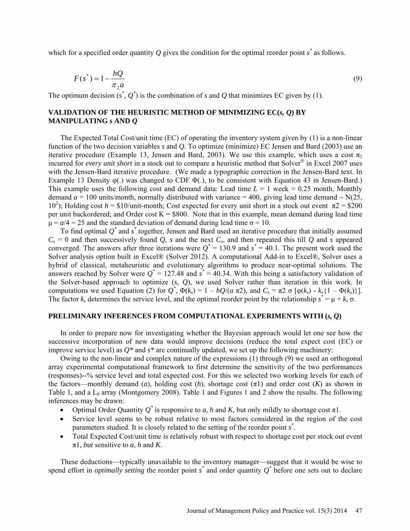
Owing to the non-linear and complex nature of the expressions (1) through (9) we used an orthogonal array experimental computational framework to first determine the sensitivity of the two performances (responses)--% service level and total expected cost. For this we selected two working levels for each of the factors—monthly demand (a), holding cost (h), shortage cost (π1) and order cost (K) as shown in Table 1, and a L8 array (Montgomery 2008). Table 1 and Figures 1 and 2 show the results. The following inferences may be drawn:

• Optimal Order Quantity Q* is responsive to a, h and K, but only mildly to shortage cost π1. • Service level seems to be robust relative to most factors considered in the region of the cost

parameters studied. It is closely related to the setting of the reorder point s*. • Total Expected Cost/unit time is relatively robust with respect to shortage cost per stock out event

π1, but sensitive to a, h and K. These deductions—typically unavailable to the inventory manager—suggest that it would be wise to

spend effort in optimally setting the reorder point s* and order quantity Q* before one sets out to declare


the operational policies of an inventory system to cope with stochastic demand. In one sense, this information is similar to the relative robustness of the total operating cost/unit time to EOQ for a deterministic inventory system. Limited generalization of such deductions may be attempted in a given cost-demand scenario to assess how accurately the parameters a, h, K and π1 need to be estimated, to assure minimum cost operation of the inventory system. In this study we focus on the factor with perhaps the highest uncertainty—the stochastic nature of X, the demand per unit time.

TABLE 1 AN L8 COMPUTATIONAL EXPERIMENT TO UNCOVER THE SENSITIVITY OF SERVICE

LEVEL AND TOTAL EXPECTED COST OF AN (s, Q) INVENTORY SYSTEM

FIGURE 1 SENSITIVITY OF OPTIMAL REORDER POINT (s*), ORDER QUANTITY (Q*) TO

MONTHLY DEMAND RATE AND COSTS

0

50

100

150

a = 50 100 h = 5 10 π1 = 500

1000 K = 400 800

Qua

ntity

or

$

Sensitivity of (s, Q) Policy Performance to Demand Rate and Cost Factors

Reorder Point "s" Order Quantity "Q"

% Service Level

Orthogonal Experiment #

a Units /month

h

π1

K

s*

Q*

%Service Level

Total Expected Cost/unit time

1 50 5 500 400 19.25 91 97.2 488.76 2 50 5 1000 800 19.88 127.9 98.2 676.6 3 50 10 500 400 18.56 64.9 95.7 709.93 4 50 10 1000 800 19.25 91 97.2 977.51 5 100 5 500 800 33.61 181.2 95.74 949.29 6 100 5 1000 400 36.22 128.4 98.76 698.3 7 100 10 500 800 32.51 129.1 93.35 1366.1 8 100 10 1000 400 35.41 91.5 98.13 1019.2


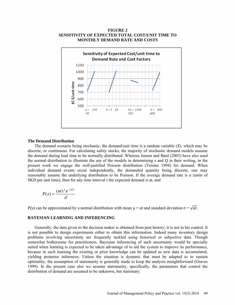
FIGURE 2 SENSITIVITY OF EXPECTED TOTAL COST/UNIT TIME TO

MONTHLY DEMAND RATE AND COSTS

The Demand Distribution The demand scenario being stochastic, the demand/unit time is a random variable (X), which may be

discrete, or continuous. For calculating safety stocks, the majority of stochastic demand models assume the demand during lead time to be normally distributed. Whereas Jensen and Bard (2003) have also used the normal distribution to illustrate the use of the models in determining s and Q in their writing, in the present work we engage the well-justified Poisson distribution (Tersine 1994) for demand. When individual demand events occur independently, the demanded quantity being discrete, one may reasonably assume the underlying distribution to be Poisson. If the average demand rate is a (units of SKD per unit time), then for any time interval t the expected demand is at, and

!)()(

)(

xeatxP

atx −

=

P(x) can be approximated by a normal distribution with mean μ = at and standard deviation σ = √𝑎𝑡. BAYESIAN LEARNING AND INFERENCING

Generally, the data given to the decision maker is obtained from past history; it is not in his control. It

is not possible to design experiments either to obtain this information. Indeed many inventory design problems involving uncertainty are frequently tackled using historical or subjective data. Though somewhat bothersome for practitioners, Bayesian inferencing of such uncertainty would be specially suited when learning is expected to be taken advantage of to aid the system to improve its performance, because in such learning the existing or prior knowledge can be updated as new data is accumulated, yielding posterior inferences. Unless the situation is dynamic that must be adapted to to sustain optimality, the assumption of stationarity is generally made to keep the analysis straightforward (Graves 1999). In the present case also we assume stationarity; specifically, the parameters that control the distribution of demand are assumed to be unknown, but stationary.


Since the Bayesian learning logic (prior prior + data posterior) follows the path of pre-supposing information, observing the phenomena and then repeatedly updating stochastic information, it is important here to select an appropriate subjective probability function for the “prior”. Indeed it is often difficult to find a suitable family of prior distributions that would help one to capture the decision maker’s subjective belief, and also be algebraically workable to produce the “posterior” as new data is received. In theory this is done by deriving the posterior density from the likelihood function and the prior density, and deriving the distribution of the reduced-form parameters from the initial information on the unknown parameters controlling the stochastic process (here the random occurrence of demand).

For the present case, therefore, demand is being assumed to be random, Poisson distributed with an unknown parameter (average rate) λ/unit time. This assumption has two advantages: First, the Poisson distribution is often quite realistic when the quantities demanded are random and independent of earlier and future demands. Secondly, from analytical point of view, the Bayesian prior-posterior conjugate family (Raiffa and Schlaifer 1961) of the distribution of the possible values of λ is Gamma, a two-parameter distribution that is convenient to update. However, we note that this is not a major restriction—Bayesian inference may be performed using stochastic simulation of the process also (Morales et al. 2005).

The Bayesian Learning Framework

Poisson being the assumed distribution controlling demand with an unknown stationary rate λ/unit time, we will treat this uncertainty as a prior probability distribution, to be updated as a posterior distribution on the basis of new demand data as observed. The conjugate prior distribution for the Poisson rate parameter is the Gamma distribution with two parameters α and β, the density function being

0,0,0,)(

)( 1 >>≥Γ

= −− βααβ βα

α

xexxGamma x

where ∫∞

−−=Γ0

1)( dtet tαα .

In Bayesian statistics, the Gamma distribution is used as a conjugate prior (Raiffa and Schlaifer 1961) distribution for various types of rate parameters, such as the λ of an exponential distribution or a Poisson distribution. The Gamma distribution has a mean of α/β, variance α/β2 and it is known to be flexible in shape. The interpretation is as follows: There are α total occurrences in β time intervals. Updating the Gamma prior is straightforward. For instance, if r quantities are demanded from the inventory in a time period of length t, the posterior density of λ will be a Gamma distribution with α’ = α + r and β’ = β + t. The maximum likelihood estimated of λ is obtained from the posterior mean

trE

++

=βαλ)(

This posterior mean E(λ) approaches MLEλ in the limit as α 0 and β 0. In the present application

our intention will be to start with some reasonably assumed prior value of Poisson demand rate λ (= α/β) and then continually update it using r (the demand observed in the time span t) as time t progresses.

The Bayesian approach to updating modeling parameters, such as the random demand that an inventory should be capable of satisfying, gives us a way around a special decision problem. In many such cases the object is to make the best decision on the basis of a given set of data (Lancaster 2004). This data may be available from past history, or it may be produced by conducting some special statistical experiments. What if there is no such history available, or there is no opportunity to conduct the desired experiments? As said above, the Bayesian approach begins with an assumed prior about the decision environment, and then by using a learning logic (prior prior + data posterior) follows the path of pre-supposing information, observes the phenomena and then repeatedly updates the information at hand (see Brown and Rogers 1972, Aronis et al. 2004, Morales et al. 2005).


FIGURE 3 TRACE OF CONTINUALLY UPDATED POSTERIOR MEAN ESTIMATES PRODUCED BY

SUCCESSION OF SAMPLES DRAWN FROM A SIMULATED POISSON DISTRIBUTION WITH λ = 100

Figure 3 and Table 2 display the effect of updating the maximum likelihood estimate of the mean

demand of a Poisson distribution. In this case a Poisson demand process with true mean demand (λ) of 100 units/month was observed (simulated) in succession of months 1, 2, 3, … etc. and the estimates of the posterior along with the ±95% limits of this estimate was calculated. The prior of λ was assumed to be a Gamma(α = 5, β = 1) distribution with an average of 5 units/month. The simulated monthly demands are shown in the second column (ki) of Table 2. Continual updating of the estimated value of λ produced a 95% confidence band for λ as (96.81, 100.77) after 100 updates. Clearly, another assumed value of the prior would produce another trace of estimates. But it can be assured based on the standard deviation of the estimated λ that they would all eventually converge toward the true demand as time t increases. REGULAR BAYESIAN UPDATES OF DEMAND RATE HELP KEEP TOTAL EXPECTED COST NEAR MINIMUM

It is clear from the foregoing section that when demand is unknown and stochastic, the original

assumption about demand shifts gradually toward the true demand when the estimate of the true demand is suitably updated. One method for accomplishing this would be to incorporate Bayesian learning. This section adds in Bayesian learning into the (s, Q) policy to help evaluate the utility of doing this. Such learning would help in moving the operating values of the two decision parameters—s, the reorder point, and Q, the order quantity—closer to their optimal values as time advances and new demand data become known. For effectively using the (s, Q) policy the motivation for continually adjusting s and Q therefore would be to keep the total expected inventory management cost near its minimum throughout the period for which the inventory is maintained and managed.

0.00

20.00

40.00

60.00

80.00

100.00

120.00 1 6 11

16

21

26

31

36

41

46

51

56

61

66

71

76

81

86

91

96

Simulated Posterior Poisson Mean Demand, True λ = 100/month

Prior assumed to be Gamma(5,1)

Mean estimated 95% upper limit 95% lower limit


TABLE 2 100 POISSON RANDOM VALUES SIMULATED WITH λ = 100. ASSUMING A PRIOR AS A

GAMMA(α = 5, β = 1) DISTRIBUTION, WE COMPUTE MEAN OF THE GAMMA POSTERIOR DISTRIBUTIONS AS MONTHLY DEMAND IS SUCCESSIVELY OBSERVED

Month # Observed Monthly Demand

For Posterior

Gamma (α, β): λ = Mean of Gamma

Posterior

SD =

SQRT(α/β2)

Upper/Lower estimates of λ

i ki Sum ki α = α + sum ki β = β + n λ estimate = α/β SD (λ est) +95% -95% Month 1 111 111 116 2 58.00 5.39 68.77 47.23

2 111 222 227 3 75.67 5.02 85.71 65.62 3 92 314 319 4 79.75 4.47 88.68 70.82 4 104 418 423 5 84.60 4.11 92.83 76.37 5 102 520 525 6 87.50 3.82 95.14 79.86 6 98 618 623 7 89.00 3.57 96.13 81.87 7 103 721 726 8 90.75 3.37 97.49 84.01 8 92 813 818 9 90.89 3.18 97.24 84.53 9 100 913 918 10 91.80 3.03 97.86 85.74 10 99 1012 1017 11 92.45 2.90 98.25 86.66 11 90 1102 1107 12 92.25 2.77 97.80 86.70 12 95 1197 1202 13 92.40 2.67 97.80 87.13 13 103 1300 1305 14 93.21 2.58 98.37 88.05 14 108 1408 1413 15 94.20 2.51 99.21 89.19 15 91 1499 1504 16 94.00 2.42 98.85 89.15 16 94 1593 1598 17 94.00 2.35 98.70 89.30 17 109 1702 1707 18 94.83 2.30 99.42 90.24 18 92 1794 1799 19 94.68 2.23 99.15 90.22 19 102 1896 1901 20 95.05 2.18 99.41 90.69 20 95 1991 1996 21 95.05 2.13 99.30 90.79 21 96 2087 2092 22 95.09 2.08 99.25 90.93 22 101 2188 2193 23 95.35 2.04 99.42 91.28 23 116 2304 2309 24 96.21 2.00 100.21 92.20 24 110 2414 2419 25 96.76 1.97 100.69 92.83 25 112 2526 2531 26 97.35 1.93 101.22 93.48 26 88 2614 2619 27 97.00 1.90 100.79 93.21 27 97 2711 2716 28 97.00 1.86 100.72 93.28 28 96 2807 2812 29 96.97 1.83 100.62 93.31 29 105 2912 2917 30 97.23 1.80 100.83 93.63 30 99 3011 3016 31 97.29 1.77 100.83 93.75 31 89 3100 3105 32 97.03 1.74 100.51 93.55 32 111 3211 3216 33 97.45 1.72 100.89 94.02 33 102 3313 3318 34 97.59 1.69 100.98 94.20 34 85 3398 3403 35 97.23 1.67 100.56 93.90 35 97 3495 3500 36 97.22 1.64 100.51 93.94 36 111 3606 3611 37 97.59 1.62 100.84 94.35 37 109 3715 3720 38 97.89 1.61 101.10 94.68 38 108 3823 3828 39 98.15 1.59 101.33 94.98 39 113 3936 3941 40 98.53 1.57 101.66 95.39 40 100 4036 4041 41 98.56 1.55 101.66 95.46 41 99 4135 4140 42 98.57 1.53 101.64 95.51 42 109 4244 4249 43 98.81 1.52 101.85 95.78 43 98 4342 4347 44 98.80 1.50 101.79 95.80 44 83 4425 4430 45 98.44 1.48 101.40 95.49 45 103 4528 4533 46 98.54 1.46 101.47 95.62 46 92 4620 4625 47 98.40 1.45 101.30 95.51 47 98 4718 4723 48 98.40 1.43 101.26 95.53 48 96 4814 4819 49 98.35 1.42 101.18 95.51 49 109 4923 4928 50 98.56 1.40 101.37 95.75 50 109 5032 5037 51 98.76 1.39 101.55 95.98


TABLE 2 (CONTD.) 100 POISSON RANDOM VALUES SIMULATED WITH λ = 100. ASSUMING A PRIOR AS A

GAMMA(α = 5, β = 1) DISTRIBUTION, WE COMPUTE MEAN OF THE GAMMA POSTERIOR DISTRIBUTIONS AS MONTHLY DEMAND IS SUCCESSIVELY OBSERVED

Month #

Observed Monthly Demand

For Posterior

Gamma (α, β): λ = Mean of

Gamma Posterior

SD =

SQRT(α/β2)

Upper/Lower estimates of λ

i ki Sum ki α = α + sum ki β = β + n λ estimate = α/β SD (λ est) +95% -95% 51 93 5125 5130 52 98.65 1.38 101.41 95.90 52 86 5211 5216 53 98.42 1.36 101.14 95.69 53 96 5307 5312 54 98.37 1.35 101.07 95.67 54 92 5399 5404 55 98.25 1.34 100.93 95.58 55 93 5492 5497 56 98.16 1.32 100.81 95.51 56 93 5585 5590 57 98.07 1.31 100.69 95.45 57 116 5701 5706 58 98.38 1.30 100.98 95.77 58 103 5804 5809 59 98.46 1.29 101.04 95.87 59 105 5909 5914 60 98.57 1.28 101.13 96.00 60 105 6014 6019 61 98.67 1.27 101.22 96.13 61 85 6099 6104 62 98.45 1.26 100.97 95.93 62 95 6194 6199 63 98.40 1.25 100.90 95.90 63 109 6303 6308 64 98.56 1.24 101.04 96.08 64 108 6411 6416 65 98.71 1.23 101.17 96.24 65 81 6492 6497 66 98.44 1.22 100.88 96.00 66 94 6586 6591 67 98.37 1.21 100.80 95.95 67 91 6677 6682 68 98.26 1.20 100.67 95.86 68 92 6769 6774 69 98.17 1.19 100.56 95.79 69 93 6862 6867 70 98.10 1.18 100.47 95.73 70 120 6982 6987 71 98.41 1.18 100.76 96.05 71 107 7089 7094 72 98.53 1.17 100.87 96.19 72 104 7193 7198 73 98.60 1.16 100.93 96.28 73 105 7298 7303 74 98.69 1.15 101.00 96.38 74 87 7385 7390 75 98.53 1.15 100.83 96.24 75 89 7474 7479 76 98.41 1.14 100.68 96.13 76 94 7568 7573 77 98.35 1.13 100.61 96.09 77 91 7659 7664 78 98.26 1.12 100.50 96.01 78 115 7774 7779 79 98.47 1.12 100.70 96.24 79 95 7869 7874 80 98.43 1.11 100.64 96.21 80 98 7967 7972 81 98.42 1.10 100.62 96.22 81 96 8063 8068 82 98.39 1.10 100.58 96.20 82 104 8167 8172 83 98.46 1.09 100.64 96.28 83 93 8260 8265 84 98.39 1.08 100.56 96.23 84 112 8372 8377 85 98.55 1.08 100.71 96.40 85 106 8478 8483 86 98.64 1.07 100.78 96.50 86 101 8579 8584 87 98.67 1.06 100.80 96.54 87 96 8675 8680 88 98.64 1.06 100.75 96.52 88 100 8775 8780 89 98.65 1.05 100.76 96.55 89 98 8873 8878 90 98.64 1.05 100.74 96.55 90 105 8978 8983 91 98.71 1.04 100.80 96.63 91 119 9097 9102 92 98.93 1.04 101.01 96.86 92 92 9189 9194 93 98.86 1.03 100.92 96.80 93 106 9295 9300 94 98.94 1.03 100.99 96.88 94 99 9394 9399 95 98.94 1.02 100.98 96.90 95 99 9493 9498 96 98.94 1.02 100.97 96.91 96 111 9604 9609 97 99.06 1.01 101.08 97.04 97 88 9692 9697 98 98.95 1.00 100.96 96.94 98 103 9795 9800 99 98.99 1.00 100.99 96.99 99 88 9883 9888 100 98.88 0.99 100.87 96.89

100 90 9973 9978 101 98.79 0.99 100.77 96.81


One way to operate the (s, Q) inventory policy when demand is stochastic is to be myopic (Levy et al. 2007) when one sets the operating values of s and Q at some initial (prior) guess for the demand rate λ, or perhaps collects only a limited amount of demand data and then estimates λ. Such trust on an initial guess for λ and not changing it later may even be favored, for this may save the added effort needed to incorporate any emergent evidence about true demand as the business moves forward and one becomes busy. Many practitioners indeed do not change the initial assumption about a or λ or even costs, though Azoury and Miller (1994) have amply highlighted the effect of not utilizing emerging information—by comparing Bayesian and non-Bayesian methodologies for it.

Plainly, the s and Q derived using the initial guess for λ would almost surely be suboptimal, except by accident (Figure 2 indicates the strong dependence of EC on a (hence on λ)). To test any possible merit of the myopic approach we set the course computationally. Table 3 displays the effect of setting the unknown demand rate λ at some unsubstantiated value (assuming mistakenly this to be the true demand), deriving the flawed s* and Q* from it, and incurring the consequent expected total cost EC when the (s, Q) policy is used. It is straightforward to compare these higher values of EC with the near optimal EC achievable by getting close to the true demand rate. We show this here by using the Bayesian approach. The illustration in Table 3 used 100 units/month as the true demand rate whereas the (“wrongly”) presumed values of λ were set respectively at 25, 50, 75, 150, 200, and 300 units/month. The costs used were h = $10/unit-month, π1 = $500 per backorder event and K = $800/order placed.

Figures 4 and 5 respectively display the effect of using a flawed (differing from the true) demand conjecture (“prior”) on the expected total cost (EC), and the service level experienced by customers.

TABLE 3 COSTS AND SERVICE LEVELS EXPERIENCED WHEN s* AND Q* ARE SET BASED ON A

PRIOR ESTIMATED DEMAND, BUT TRUE DEMAND (aT) IS DIFFERENT FROM THE PRIOR ESTIMATE (a)

a = Estimated demand/month based on a flawed prior guess 25 50 75 100 150 200 300

aT = True demand/month 100 100 100 100 100 100 100

s* = Optimum Reorder Point based on prior 10 18 25 33 47 61 88

Q* = Optimum Order Quantity based on prior 65 91 111 129 158 183 224

Holding Cost based on a and (s*, Q*) 360 510 624 720 883 1019 1248

Holding Cost based on (s*, Q*) but facing True demand 173 385 569 721 989 1269 1748

Replenishment Cost by a and (s*, Q*) 310 438 537 620 759 876 1073

Replenishment Cost based on (s*, Q*) but facing True demand 1239 876 715 620 506 438 358

Shortage Cost by a and (s*, Q*) 13 18 22 26 32 36 45

Shortage Cost based on (s*, Q*) but facing True demand 52 36 21 26 36 18 15

Expected Total Cost by a and (s*, Q*) 683 966 1183 1366 1673 1932 2366

Expected Total Cost based on (s*, Q*) but facing True demand 1464 1297 1305 1366 1531 1725 2121

Service level experienced at True Demand but operating at (s*, Q*)

98.8%

97.2%

95.4%

93.4%

88.5%

82.5%

59.6%


FIGURE 4 THE EXPECTED TOTAL COST FOR A (s, Q) SYSTEM THAT USES A

FLAWED PRIOR ESTIMATE THAT IS FAR FROM THE TRUE DEMAND VALUE

FIGURE 5 SERVICE LEVEL PROVIDED BY A (s, Q) SYSTEM THAT USES A

FLAWED PRIOR ESTIMATE THAT IS FAR FROM THE TRUE DEMAND VALUE

50.0%

55.0%

60.0%

65.0%

70.0%

75.0%

80.0%

85.0%

90.0%

95.0%

100.0%

Prior Demand

25/month

50 75 100 150 200 300

Serv

ice

Leve

l

% Service Level facing True Demand (= 100/month) but using (s*, Q*) based on Prior λ


A review of Table 3 and Figures 4 and 5 would suggest that the results of using Bayesian learning to keep continually updating the demand estimate provide a mixed message. But a closer look reveals that the minimum total cost (s, Q) policy should indeed be based on a demand estimate as close to the true demand as is possible. But Figure 4 appears to suggest that a lower guess for demand actually improves customer service! Prima facie, therefore, guessing a low value of demand appears to be doing something good. But such inference is shortsighted and most misleading. More seriously, this is not a defect in the model or its analysis, rather perhaps in the analyst’s formulation of the problem at hand.

Recall that our objective of setting up the (s, Q) model to help find a rational way to manage inventories when demand is stochastic included spelling out the objective first—that of minimizing (1), the expected total cost/unit time. This total cost included three components—the holding cost, the replenishment cost, and the shortage cost. At least for this model, therefore, maximizing customer service per se was not the objective. Customer service (F(s)) enters into (1) via Cs (= π1(1 – F(s))), the cost of short shipment. If one requires the final (s, Q) solution to assure a high level of customer service, one would need to use a large value for π1. Thus, like any optimization attempted, one would need to be clear about the objective of the decision maker—where does he want to put priority?

CONCLUSIONS

This study has investigated the value of incorporating Bayesian learning into the popular (s, Q) model

for managing inventories when demand is stochastic. The study finds that one can indeed make a decent start by the Bayesian approach—and stay the course nearly optimally—while upholding a target service level by suitably selecting costs and also keeping the expected operating cost/unit time minimum. Specifically, this study uncovers the high value in continually updating the decisions (a) “when to order”, and (b) “how much to order”, rather than sticking to the initial guess for the demand average, as is frequently practiced.

Demand has been assumed to follow a stationary Poisson distribution in this work. The Bayesian learning process uses the Gamma conjugate family of distributions to incorporate the latest observed demand data. The learning logic follows the path prior prior + data posterior of observing and updating stochastic information.

Owing to the non-linear and complex nature of the expressions in the (s, Q) model, this work utilized an orthogonal array experimental framework to determine the sensitivity of the two performances (responses)--% service level and total expected cost. For this two working levels for each of the factors—monthly demand (a), holding cost (h), shortage cost (π1) and order cost (K) were selected and a L8 array was adopted to guide the computations. The following inferences could be drawn:

• Optimal Order Quantity Q* is affected significantly by a, h and K, but only mildly by shortage cost π1.

• Service level seems to be robust relative to most factors considered in the region of the cost parameters studied. It is closely related to shortage cost π1 and the setting of the reorder point s*.

• Total Expected Cost/unit time is relatively robust with respect to shortage cost per stock out event π1, but sensitive to a, h and K.

• A myopic estimate of the true demand rate λ would regularly turn out a suboptimal EC. These deductions—typically unavailable to the inventory manager—suggest that it would be wise to

spend effort in optimally setting the reorder point s* and order quantity Q* before one sets out to declare the operational policies to cope with stochastic demand. In a sense, this information is comparable to the knowledge of relative robustness of the total operating cost/unit time to EOQ for a deterministic inventory system (see Winston 2003, page 853).

In summary, this study, like the work of Azoury and Miller (1994) conducted for the n-period nondepletive inventory model, establishes the worth of following the Bayesian approach to update stochastic information used in the (s, Q) inventory system as new demand data become continually available. The result is lowering of the total expected cost throughout the time this inventory system is


operated. As already shown in the literature in a large number of applications, the Bayesian learning path prior prior + data posterior, it appears, would benefit the design and operation of other similar stochastic systems as well. REFERENCES Aronis, K-P, R Dekker, I Magou and G Tagaras (2004). Inventory Control of Spare Parts using a

Bayesian Approache: A Case Study, European Journal of Operations Research, Vol 154(3), 730-739.

Azoury Katy S and Bruce L Miller (1994). A Comparison of the Optimal Ordering Levels of Bayesian and Non-Bayesian Inventory Models, Management Science.

Bagchi, Tapan P and A A Cunnigham (1972). Bayesian Approach to the Design of Queuing Systems, INFOR Journal, Vol 10(1).

Brown Jr, G F and W F Rogers (1973). A Bayesian approach to demand estimation and inventory provisioning, Naval Research Logistics Quarterly, Vol 20(4), 607–624, December.

Graves, Stephen C (1999). A Single-Item Inventory Model for a Nonstationary Demand Process, Manufacturing & Service Operations Management, Vol 1(1), 50-61.

Huh, W T, R Levi, P Rusmevichientong and J Orlin (2010). Adaptive data-driven inventory control policies based on Kaplan-Meier estimator for censored demand, Operations Research, Vol 59, 929-941.

Huh, W T and P Rusmevichientong (2009). A nonparametric asymptotic analysis of inventory planning with censored demand, Mathematics of Operations Research, Vol 34, 821-839.

Jensen, P A and J F Bard (2003). Operations research: Models and Methods, John Wiley & Sons Inc. Lancaster, Tory (2004). An Introduction to Modern Bayesian Econometrics, Blackwell. Levi, T, R O Roundy and D B Shmoys (2007). Provably near-optimal sampling-based policies for

stochastic inventory control models, Operations Research, Vol 32, 821-839. Montgomery, D C (2008). Design and Analysis of Experiments, 5th ed., John Wiley. Morales, J, M E Castellanos, A M Mayoral and C Armero (2005). Bayesian Design in Queues: An

Application to Aeronautic Maintenance, Centro de Investigacion Operative, Elche. Murray, George R and Edward A Silver (1966). A Bayesian Analysis of the Style Goods Inventory

Problem, Management Science, 1966, vol. 12 (11), pages 785-797. Peterson R and E A Silver (1979). Decision Systems for Inventory Management and Production

Planning, John Wiley. Prabhu, N U (1965). Queues and Inventories: A Study of Their Basic Stochastic Processes, John Wiley. Raiffa, Howard and Robert Schlaifer (1961). Applied Statistical Decision Theory. Division of Research,

Graduate School of Business Administration, Harvard University. Sharma, Sunil, C Erik Larson and Lars J O (2001). Optimal Inventory Policies when the Demand

Distribution is not Known, Journal of Economic Theory, Vol. 101, No. 1, pp. 281-300, November. Silver, E A (1981). Operations Research in Inventory Management: A Review and Critique, Operations

Research, vol. 29 no. 4 628-645. Silver, E A, D F Pyke, R Peterson (1998). Inventory Management and Production Planning and

Scheduling, Wiley Silver, E A (2007). Inventory Management: A Tutorial 2007-03, University of Calgary. Solver (2012). Optimization Methods, www.solver.com, Frontline Systems Inc. Tersine, R J (1994). Principles of Inventory and Materials Management (4th ed.), Prentice-Hall. Tim Huh, Woonghee, Retsef Levi, Paat Rusmevichientong and James B Orlin (2012). Adaptive Data-

Driven Inventory Control with Censored Demand Based on Kaplan-Meier Estimator, Operations Research, July/August 2011 vol. 59 no. 4, 929-941

Tim Huh, Woonghee and Paat Rusmevichientong (2009). A Nonparametric Asymptotic Analysis of Inventory Planning with Censored Demand.

Winston, W L (2003). Operations Research: Applications and Algorithms, Cengage Learning.


bayesian design of inventory systems to minimize expected ... · bayesian design of inventory...

Documents