bayesian analysis of climate change impacts in phenology · bayesian analysis of climate change...

Bayesian analysis of climate change impacts inphenology

V O L K E R D O S E * a n d A N N E T T E M E N Z E L w*Centre for Interdisciplinary Plasma Science, Max-Planck-Institut fur Plasmaphysik, EURATOM Association, Boltzmannstrasse 2,

D-85748 Garching bei Munchen, Germany, wDepartment of Ecology, Center of Life Science, TU Munich, Am Hochanger 13,

D-85354 Freising, Germany

Abstract

The identification of changes in observational data relating to the climate change

hypothesis remains a topic of paramount importance. In particular, scientifically sound

and rigorous methods for detecting changes are urgently needed. In this paper, we

develop a Bayesian approach to nonparametric function estimation. The method is

applied to blossom time series of Prunus avium L., Galanthus nivalis L. and Tiliaplatyphyllos SCOP. The functional behavior of these series is represented by three

different models: the constant model, the linear model and the one change point model.

The one change point model turns out to be the preferred one in all three data sets with

considerable discrimination of the other alternatives. In addition to the functional

behavior, rates of change in terms of days per year were also calculated. We obtain also

uncertainty margins for both function estimates and rates of change. Our results provide

a quantitative representation of what was previously inferred from the same data by less

involved methods.

Keywords: Bayesian theory, climate change, phenology, trend

Received 12 June 2003; revised version received and accepted15 September 2003

Introduction

The global average surface temperature has increased

over the 20th century by about 0.6 � 0.2 1C and is

projected to continue to rise at a rapid rate. However,

the record shows a great deal of variability: Most of the

warming has occurred during two periods (1910–1945

and 1976–2000) and it is very likely that the 1990s were

the warmest decade (IPCC, 2001). Many studies have

revealed evidence of ecological impacts of this recent

climate change. In particular, shifts in plant and animal

phenology for the boreal and temperate zones of the

northern hemisphere have been reported (Menzel &

Estrella, 2001; Sparks & Menzel, 2002; Walther et al.,

2002; Root et al., 2003). Phenology is perhaps the

simplest and most frequently used bio-indicator to

track climate changes. Springtime phases are particu-

larly sensitive to temperature. Thus, phenological

observations can demonstrate a consistent tempera-

ture-related shift or ‘fingerprint’ and assess the amount

of change. Reviews of phenological trend studies

indicate that most of the data originate from the last

four to five decades. These recent data predominantly

reveal advancing of flowering and leaf unfolding in

Europe and North America by 1.2–3.8 days decade�1 on

average and a strong seasonal variation with highest

advances in early spring.

However, there are several problems involved in the

commonly used methods of searching for signals in

phenological time series. The detection of shifts is

mostly done by classical statistical methods, such as

slopes of linear regression models (e.g. Bradley et al.,

1999; Menzel & Fabian, 1999; Jones & Davis, 2000;

Schwartz & Reiter, 2000; Defila & Clot, 2001; Menzel

et al., 2001; Ahas et al., 2002; Penuelas et al., 2002;

Menzel, 2003), rarely by other curve fitting methods

(e.g. Ahas, 1999; Sagarin & Micheli, 2001). Trends are

then reported in days per year or decade, or days of

change over the study period. The above methods are

sensitive to extreme values (Schlittgen & Streitberg,

1999). It is apparent that using linear regression models

the length of a time series and its start and end dates are

critical in detecting changes and in determining their

magnitude, especially when highly variable phenologi-

cal time series of a few decades are analyzed. Thus,Correspondence: Prof. Dr. Volker Dose, tel. 1 49 89 3299 1265, fax

1 49 89 3299 2591, e-mail: [email protected]

Global Change Biology (2004) 10, 259–272, doi: 10.1111/j.1529-8817.2003.00731.x

r 2004 Blackwell Publishing Ltd 259

series that include the whole of the 1990s benefit from

the decade being the warmest on record. However, the

observation periods vary between phenological net-

works and among stations in networks because

phenological observations mostly depend on volun-

teers and thus have often discontinuous, incomplete

data series. Moreover, different individuals may apply

different standards in their observations. Several

studies have addressed this problem (e.g. Menzel &

Estrella, 2001; Sparks & Menzel, 2002) and illustrate the

variation of resulting changes with the period of

interest (e.g. Scheifinger et al., 2002). Few studies use

these linear regression models for even longer time

series, some covering almost one century (Beaubien &

Freeland, 2000; Kozlov & Berlina, 2002; Magnuson et al.,

2000 as well as Sagarin & Micheli, 2001 for lake and

river ice cover).

Reviews of phenological trend studies suggest that

only about 40% of the reported trends have proved

statistically significant. The significance is often tested

by the F-test (Defila & Clot, 2001), and occasionally by

the Mann–Kendall trend test, which does not require a

Gaussian distribution of the data (e.g. Menzel, 2000).

Few studies also report the standard error of the slope

(e.g. Sagarin, 2001).

Studies analyzing long-term phenological records

often reveal a heterogeneous pattern of temporal

variability with sometimes alternating periods of

advanced and delayed onset (e.g. Schnelle, 1950;

Lauscher, 1978, 1983; Freitag, 1987; Sparks & Carey,

1995; Ahas, 1999). The advance of phenological events

in the last decades is compared to the timing in

preceding periods, mostly only by comparing averages

in distinct periods (e.g. Fitter & Fitter, 2002). Another

phenomenon in time domain described (Chmielewski

& Rotzer, 2002; Scheifinger et al., 2002) is a discontinuity

in time series behavior in the late 1980s, as in many

areas almost no trend is observed before the discontin-

uous shift towards earlier occurrence dates after the late

1980s. However, change points have not been deter-

mined so far in phenological time series.

These limitations of the currently used methods

render comparison and interpretation of the observed

changes extremely difficult. They may partly account

for the observed spatial variability among sites or the

different response of species besides the inherent

inhomogeneity caused by local microclimate condi-

tions, natural variation, genetic differences or other

nonclimatic factors. Thus, there is strong need to

improve the recently applied method of change detec-

tion in phenological time series.

Although we are familiar with the ongoing battle

between traditional statisticians and the (much older,

Bayes, 1763) Bayesian school of thought, we shall not

add to the many existing comments. Bayesian methods

are presently undergoing an impressive renaissance

since the computational problems involved in the

application of Bayes theorem fade away with the ever

more powerful personal computers available to every

scientist. We identify ourselves as practising Bayesians

(Dose, 2003) for the reason that this theory of

probability requires to make explicit all assumptions

that enter the analysis of a particular data set.

Furthermore, the marginalization option of Bayesian

probability theory, which has no satisfactory counter-

part in traditional frequentist statistics, is of invaluable

importance in the case of incomplete or poorly

conditioned data. Such data sets may be associated

with complicated, even multimodal likelihoods (see

Discussion). Rigorous application of Bayesian methods

allows also for a rigorous analysis of uncertainties of

the results. The importance of uncertainty analysis in

climate-related research has recently been vigorously

pointed out by Katz (2002). We deem equally important

the model comparison option of Bayesian probability

theory. There is no such thing as a null hypothesis in

Bayesian theory. Instead, the theory allows for a

ranking of a bunch of models (at least two !) and

provides numerical measures of their respective prob-

abilities. The model comparison option of Bayesian

theory rests on the built-in Ockham’s razor (Garrett,

1991), which limits the complexity of a model to the

amount necessary to explain the data, avoiding the

fitting of noise. The analysis in the section on Model

selection will compare three different models for the

trend of flowering time series.

Bayesian statistical methods have been applied so far

in climate change detection, analysis and attribution

(e.g. Hobbs, 1997; Hasselmann 1998; Leroy, 1998; Tol &

De Vos, 1998; Barnett et al., 1999; Berliner et al., 2000;

Katz, 2002), and, for example, in climate reconstructions

(Robertson et al., 1999). Previous work on model

comparison addressed the test for changes in mean

and/or variance in hydrological data (Perreault et al.,

2000).

In this study, we will focus on long-term phenological

observations (1896–2002) in Germany and analyze the

variations of the onset of phenological phases in the

20th century. We chose time series from Geisenheim

(491590N,71580E, 60 km west of Frankfurt am Main)

where several phenological phases have been reported

almost continuously since 1896. Three phases within

the course of the phenological year were selected. These

are: flowering of snowdrop (Galanthus nivalis L.) in

earliest spring, sweet cherry (Prunus avium L.) in mid-

spring, and lime tree (Tilia platyphyllos SCOP) in mid-

summer. Data result from the Historical Phenological

Database (1896–1935) and the Actual Phenological

260 V. D O S E & A . M E N Z E L

r 2004 Blackwell Publishing Ltd, Global Change Biology, 10, 259–272

Database (1951–2002) of the German Weather Service,

as well as from Schnelle & Witterstein (1952) (1936–

1944), and corresponding meteorological yearbooks

(1945–1952).

In the next section, we shortly introduce the Bayesian

concepts. In the subsequent section we perform a

comparison of different models to describe the func-

tional behavior of the blossom time series. The

predictions based on the best model are presented in

the penultimate section. Finally, an extention of the

analysis to other species and the discussion of the

results are presented.

Bayesian concepts

In this paper, we are concerned with the identification

of trends in phenological data. Since there is no first-

principles-based theory for such trends the method of

choice is nonparametric function estimation within the

Bayesian framework. We shall introduce the Bayesian

concepts and terminology only to the extent that is

necessary to fix the nomenclature in the rest of the

article. Readers without knowledge of Bayesian prob-

ability theory are referred to the amply available

literature for a more detailed introduction (Tribus,

1969, Box & Tiao, 1973, Sivia, 1996, Leonard & Hsu,

1999).

Bayesian probability theory is based on the applica-

tion of two rules. The first is the product rule, which

allows a probability or probability density function of

two (or more) variables conditional on additional

information I to be broken down into simpler functions:

pðy;DjIÞ ¼ pðyjIÞpðDjy; IÞ: ð1Þ

The distributions pðyjIÞ and pðDjy; IÞ depend only on

the single variables y and D, respectively. We shall

identify y with ‘parameter’ and D with ‘data’ later on.

pðyjIÞ is conditional on I only while pðDjy; IÞ is in

addition conditional on y. Because of the symmetry in

y, D of the left-hand side of Eqn (1) it may be expanded

alternatively:

pðy;DjIÞ ¼ pðDjIÞpðyjD; IÞ: ð2Þ

Equating the two equivalent expansions (1) and (2) we

arrive at Bayes theorem:

pðyjD; IÞ ¼ pðyjIÞpðDjy; IÞ=pðDjIÞ: ð3Þ

Bayes theorem tells us how to update knowledge about

the parameter y encoded in pðyjIÞ by collecting

appropriate data D. pðyjIÞ is called the prior probability

on y, which we may also regard as expert knowledge. It

can stem from earlier experiments, other observations

or evolve from the experience of the scientist working

in the respective field. pðyjIÞ is usually very weak

information. In fact, it is the large uncertainty about y

usually associated with pðyjIÞ, which motivates new

experiments or observations. The prior pðyjIÞis com-

bined with pðDjy; IÞ, the sampling distribution of the

data, to arrive at the posterior distribution of y; pðyjD; IÞgiven the new data D. pðDjy; IÞ will in the following be

regarded as a function of the parameter y and is then

called the likelihood function.

The last quantity to be explained in (3) is pðDjIÞ. It

follows from the second rule governing Bayesian

probability theory, the marginalization rule. This

extremely important rule tells how to remove an

unwanted ‘nuisance’ parameter from a Bayesian calcu-

lation:

pðDjIÞ ¼Z

pðy;DjIÞdy ¼Z

pðyjIÞpðDjy; IÞdy: ð4Þ

Comparison with (3) shows that pðDjIÞ is the normal-

ization in Bayes theorem. Eqn (4) suggests, however, an

even more extensive interpretation of pðDjIÞ. The

meaning of the parameter y is of course derived from

a function or rather a class of functions chosen to model

the data. pðDjIÞ represents then the probability of the

data given this class of functions regardless of which

numerical value the parameter y assumes. pðDjIÞ is

therefore also called the evidence of the data given a

class of models and is the key quantity to decide how to

rank a certain number of models when tried on the

same set of data. The procedure is formally simple.

Consider the models {Mj}. We then want to calculate

pðMjjD; IÞ, which is given by Bayes theorem as

pðMjjD; IÞ ¼ pðMjjIÞpðDjMj; IÞ=pðDjIÞ ð5Þ

pðDjIÞ follows as before from marginalization with the

integral in (4) replaced by a sum.

Comparison of models Mj and Mk yields the odds

ratio:

pðMjjD; IÞpðMkjD; IÞ ¼

pðMjjIÞpðMkjIÞ

pðDjMj; IÞpðDjMk; IÞ

ð6Þ

It is composed of two factors. The first is

pðMjjIÞ=pðMkjIÞ and is called the prior odds. It

summarizes the experts preference of model choice Mj

over model choice Mk. This factor is frequently taken

equal to unity since it is exactly the inability to prefer

one model against another that enforces collection of

new data. The second factor is called the Bayes factor.

The probabilities entering the Bayes factor are obtained

employing the marginalization rule:

pðDjMj; IÞ ¼Z

pðy;DjMj; IÞdy

¼Z

pðyjMj; IÞpðDjy;Mj; IÞdy:ð7Þ

We shall now approximate Eqn. (7) in order to perform

a qualitative discussion of the Bayes factor (Gregory &

C L I M AT E C H A N G E I M PA C T S 261


Loredo, 1992). We shall assume that the prior prob-

ability on y, pðyjMj; IÞ is rather uninformative and wide

in contrast to the likelihood, which we assume to be

very informative on y in which case pðDjy;Mj; IÞ is a

function that is concentrated in a narrow region Dyaround its maximum y. The integral in (7) can then be

written approximately as

pðDjMj; IÞ ¼ pðyyjMj; IÞpðDjyy;Mj; IÞDy: ð8Þ

Since the prior is a normalized function, we can define a

prior range dy by 1 ¼ dypðyyjMj; IÞ and obtain

pðDjMj; IÞ � pðDjyy;Mj; IÞDydy

: ð9Þ

The arguments above hold of course also if y is not a

scalar, i.e. even if we assume that Mj has a j-

dimensional parameter vector ~yyj. The second factor in

(9) must then be raised to the jth power. The

approximation discussed so far allows an important

conclusion for the case of nested models. We call Mj

and Mk nested if all parameters entering Mj also enter

Mk with the same meaning and prior probabilities and

k4j. The Bayes factor for this case becomes then

pðDjMj; IÞpðDjMk; IÞ

¼pðDj yyj;Mj; IÞpðDj yyk;Mk; IÞ

Dydy

� �j dyDy

� �k

: ð10Þ

According to the assumption that the prior in (7) is

rather diffuse while the likelihood is sharply peaked,

we have that Dy � dy. Since by assumption k4j the

volume factor (dy)k�j/(Dy)k�j is large compared to unity.

On the other hand, since k4j model Mk is expected to

give a better fit to the data than model Mj and

consequently pðDj yyj;Mj; IÞ=pðDj yyk;Mk; IÞ is a number

smaller than unity. Therefore, model Mk will only be

preferred over model Mj if the fit is so much better that

it overrides the volume factor. This important built-in

feature of Bayesian probability theory is called Ock-

ham’s razor. This philosophical concept requires that

one should take the simpler of two models, which both

provide reasonable explanations of the data.

Finally we comment on the importance of priors in

model comparison. The assumption above was that the

prior distribution be rather diffuse so that it hardly

influences the most probable parameter value yy.

However, if the prior range dy becomes too large or

tends even to infinity, then it follows from (10) that

always the simplest model would win the competition.

As a consequence one should try hard to formulate as

informative priors as possible for the purpose of model

comparison. Improper priors are entirely useless in this

context.

Having identified the appropriate model to explain

the data we are left with the determination of the

parameters, which specify the model. The full informa-

tion on the parameters is of course contained in the

posterior distribution (3). If it is sufficiently ‘simple’,

meaning that pðyjD; IÞ resembles a Gaussian function,

then it may be summarized in terms of mean and

variance

hyi ¼Z

ypðyjD; IÞdy;

hDy2i ¼Z

ðy� hyiÞ2pðyjD; IÞdy:ð11Þ

This completes a Bayesian analysis if the problem was

model selection and best estimate of parameters that

specify the model. Frequently, however, the problem

arises to make predictions on the basis of the available

set of data. We shall defer the treatment of this problem

to a separate section.

Model selection

The Bayesian tools will now be applied to the analysis

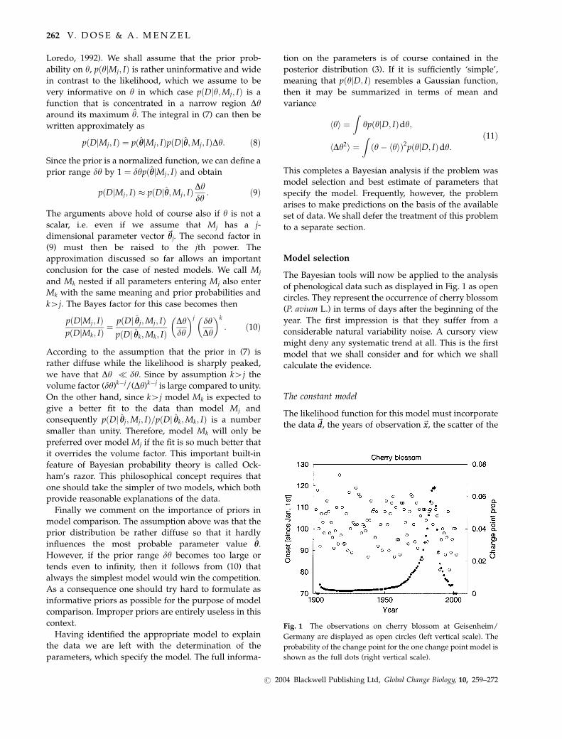
of phenological data such as displayed in Fig. 1 as open

circles. They represent the occurrence of cherry blossom

(P. avium L.) in terms of days after the beginning of the

year. The first impression is that they suffer from a

considerable natural variability noise. A cursory view

might deny any systematic trend at all. This is the first

model that we shall consider and for which we shall

calculate the evidence.

The constant model

The likelihood function for this model must incorporate

the data ~dd, the years of observation ~xx, the scatter of the

Fig. 1 The observations on cherry blossom at Geisenheim/

Germany are displayed as open circles (left vertical scale). The

probability of the change point for the one change point model is

shown as the full dots (right vertical scale).

262 V. D O S E & A . M E N Z E L


data that will be characterized by a variable s and the

constant f that we choose to define the ‘no trend’

blossom day. The model equation reads

di � f ¼ ei; 8i: ð12Þ

If expectation value heii of the errors is zero and

variance he2i iis assumed to be known as s2, then by the

principle of maximum entropy (Jaynes, 1957a, b; Kapur

& Kesavan, 1992) the explicit form of the likelihood

becomes

pð~ddj~xx; s; f ; IÞ ¼ 1

sffiffiffiffiffiffi2p

p� �N

exp � 1

2s2

XN

i

ðdi � fÞ2

( ):

ð13Þ

The same expression follows if we abandon the

principle of maximum entropy and make the much

stronger assumption that the ei follow a Gaussian

distribution with zero mean and variance s2. From (13)

we must now calculate the evidence pð~ddj~xx; c; IÞ. An

additional c has been split off from the general

conditional background I to make explicit that we treat

the constant model here. The evidence is obtained from

the marginalization theorem (4):

pð~ddj~xx; c; IÞ ¼Z

df dsp ð~dd; f ; sj~xx; c; IÞ: ð14Þ

This equation is an identity. The integrand in (14) will

now be expanded using the product rule:

pð~ddj~xx; c; IÞ ¼Z

df dspðf ; sj~xx; c; IÞ pð~ddj~xx; f ; s; c; IÞ: ð15Þ

The first distribution under the integral in (15) is

logically independent of ~xx and c and simplifies to

pðf ; sjIÞ ¼ pðsjIÞpðf js; IÞ: ð16Þ

Again logical independence applies to pðf js; IÞ since the

estimate of the average value f is not influenced by any

knowledge about the variance s2. The prior distribution

pðf jIÞ on f is then chosen (weakly informative) to be

constant over the range 2g

pðf jIÞ ¼ 1

2g: ð17Þ

The range g can be estimated from the variance of the

data in Fig. 1. A possible k-dimensional generalization

of (17) would be (1/2g)k. A more parsimonious choice

of the prior volume is, however, obtained if we replace

the hypercube by a hypersphere Vs(k,g):

Vsðk; gÞ ¼ gkðffiffiffip

pÞk=G

k þ 2

2

� �¼ pð~ff jg; k; IÞ: ð18Þ

A similar uninformative choice is made for pðsjIÞ. Since

s is a scale parameter for the difference jdi � f j, we

choose a normalized form of Jeffreys’ prior:

pðsjb; IÞ ¼ 1

2 ln b1

s;

1

b<s <b ð19Þ

The integrand in (15) is thereby fully specified. In order

to perform the integration we rewrite the exponent:Xi

ðdi � fÞ2 ¼ Nðf � dÞ2 þ NDd2; ð20Þ

d ¼ 1

N

XN

i

di; Dd2 ¼ 1

N

XN

i

ðdi � dÞ2: ð21Þ

This leads to the marginal likelihood:

pð~ddj~xx; c; IÞ ¼ 1

2p

� �N=2 1

2g1

2lnb

�Z

dss

1

sNexp �NDd2

2s2

( )

�Z

exp � N

2s2ðf � dÞ2

� �df :

ð22Þ

Although the priors on f and s have only finite range

we assume that the ranges are sufficiently large such

that the limits of integration can be extended to (0, 1)

for s and (�1, 1) for f, respectively, with negligible

approximation error on the integrals. The inner integral

is then of the standard Gaussian one-dimensional type

and yieldsZ1�1

df exp � N

2s2ðf � dÞ2

� �¼ s

ffiffiffiffiffiffi2pN

r: ð23Þ

The remaining integral can be converted to the integral

representation of the gamma function by substitution

x5 1/s2 and yieldsZ10

dss

1

sN�1exp �NDd2

2s2

( )¼ 1

2

GððN � 1Þ=2ÞfNDd2=2gðN�1Þ=2

ð24Þ

Collecting terms the evidence for the constant model

becomes

pð~ddj~xx; c; IÞ ¼ 1

2

1

p

� �ðN�1Þ=2 1

2g1

2lnbGððN � 1Þ=2ÞfNDd2gðN�1Þ=2

1ffiffiffiffiN

p :

ð25Þ

The linear model

This model assumes a linear trend in the data leaving

open the question whether we expect a rise or a fall as a

function of observation year. The model equation for

this case becomes

di � f1xN � xi

xN � x1� fN

xi � x1

xN � x1¼ ei; ð26Þ

where x1, xN are the first and last year of observation

and f1, fN design functional values that specify a linear

trend between x1 and xN but are of course unknown.

Eqn (26) suggests to go over to matrix notation:

~dd �A~ff ¼~ee: ð27Þ



Keeping assumptions on ei as before the likelihood

becomes

pð~ddj~xx; s;~ff ; l; IÞ ¼ 1


p� �N

� exp � 1

2s2ð~dd �A~ffÞTð~dd �A~ffÞ

� �:

ð28Þ

The explicitly added l in the condition reminds that we

are treating a linear trend model. The arguments that

lead to priors on ~ff and s as well as considerations of

logical independence remain unchanged. The evidence

becomes then

pð~ddj~xx; l; IÞ ¼Z

pð~ff jIÞpðsjIÞpð~ddj~xx;~ff ; s; IÞd~ff ds: ð29Þ

The main difference compared to the previous model is

that the ~ff-integration has become two dimensional.

Accordingly the rewriting of the exponent f is slightly

more complicated now. We define vector ~ff0 , matrix Q

and residue R by the equation

f ¼ ð~dd �A~ffÞTð~dd �A~ffÞ¼ ð~ff �~ff0Þ

TQð~ff �~ff0Þ þ R:ð30Þ

The~ff-integral is now straightforward and we obtain

pð~ddj~xx; l; IÞ ¼ 1

2p

� �N=2 1

Vsð2; gÞ1

2lnb

�Z10

dss

1

s2exp � R

2s2

� �2ps2ffiffiffiffiffiffiffiffiffiffiffiffiffidet Q

p :

ð31Þ

The remaining s-integral is of the same type as before

and the evidence becomes

pð~ddj~xx; l; IÞ ¼ 1

2

1

Vsð2; gÞ1

2lnb1

p

� �ðN�2Þ=2

� 1ffiffiffiffiffiffiffiffiffiffiffiffiffidet Q

p G ðN � 2Þ=2ð ÞRf gðN�2Þ=2

:

ð32Þ

Matrix Q and residue R are so far unknown. These

quantities follow from a comparison of coefficients in~ff

of the two equivalent forms of f in (30):

Q ¼ ATA;

Q~ff0 ¼ AT~dd !~ff0 ¼ Q�1AT~dd;

R ¼~ddT~dd �~dd

TAA�1AT~dd:

ð33Þ

The expression for the residue R can be simplified

considerably if we employ singular value decomposi-

tion on the matrix A. Assume

A ¼X

i

li~UUi

~VVT

i : ð34Þ

This yields for matrix Q:

Q ¼ ATA ¼X

i;k

lilk~VVi

~UUT

i~UUk

~VVT

k

¼X

k

l2k~VVk

~VVT

k :ð35Þ

The last equality follows from the fact that the f~UUigand

the f~VVigeach form an orthogonal normalized vector

system. From (34) and (35) we get immediately

det Q ¼Y

k

l2k ; ð36Þ

AQ�1AT ¼X

k

~UUk~UU

T

k ; ð37Þ

R ¼~ddT

I�X

k

~UUk~UU

T

k

( )~dd: ð38Þ

This completes the analysis of the linear model.

The change point model

A change point model is a natural refinement of the

linear model. With this model we represent the trend by

piecewise linear sections. The simplest case would be

one change point separating two linear sections. This

model contains four parameters: the design values at

the boundaries and at the change point, and in

addition, the parameter that specifies the position of

the change point. The model equation for the general

case is very similar to (25), namely,

di � fkxkþ1 � xi

xkþ1 � xk� fkþ1

xi � xk

xkþ1 � xk

¼ ei; xk � xi � xkþ1:

ð39Þ

The likelihood is identical to (28) expect for the

additional parameter ~EE, which specifies n change point

positions. Note that the~ff-space is (n1 2) dimensional in

this model and that

pð~ddj~xx; s;~ff ;~EE; IÞ ¼ 1


p� �N

� exp � 1

2s2ð~dd �Að~EEÞ~ffÞTð~dd �Að~EEÞ~ffÞ

� �:

ð40Þ

The matrix A depends now on the change point

positions ~EE. The formal similarity of the change point

model and the linear model allows duplication of most

of the previous analysis. The evidence that we need

now is pð~ddj~xx; n; IÞ where n is the number of change

points. It is given by

pð~ddj~xx; n; IÞ ¼X~EE

pð~dd;~EEj~xx; IÞ ¼X~EE

pð~EEjIÞpð~ddj~EE;~xx; IÞ: ð41Þ

The marginal likelihood pð~ddj~EE;~xx; IÞ can be taken from

the linear model case if we remember that determi-

nant of Q and residue R will now depend on ~EE.

264 V. D O S E & A . M E N Z E L


Hence

pð~ddj~xx; n; IÞ ¼ 1

2

1

p

� �ðN�n�2Þ=2 1

Vsðn þ 2; gÞ1

2lnb

�X~EE

pð~EEjIÞ 1ffiffiffiffiffiffiffiffiffiffiffiffiffiffiffiffiffiffiffidet Qð~EEÞ

q GððN � n � 2Þ=2ÞfRð~EEÞgðN�n�2Þ=2

:

ð42Þ

In order to proceed, we need to specify the number of

change points n and the prior probability of their

distribution pð~EEjIÞ. We shall assume a flat uninforma-

tive prior on ~EE meaning that pð~EEjIÞ � pðnjIÞ. Let m be

the number of data points by which we define a

regression problem of a straight-line segment. Of

course mmin5 3. If we have N data at hand, then the

number of ways to choose one change point out of

N�2m is

Zðn ¼ 1Þ ¼ N � 2m: ð43Þ

For each additional change point we must add a fit

region of size m. Hence

ZðnÞ ¼ ðN � ðn þ 1ÞmÞ!ðN � ðn þ 1Þm � nÞ!n! ¼ 1=pðEjIÞ: ð44Þ

Combining (43) and (45) we arrive at the evidence for

an n-change point model:

pð~ddj~xx; n; IÞ

¼ 1

2

1

p

� �ðN�n�2Þ=2 1

Vsðn þ 2; gÞ1

2lnb

�X~EE

n!ðN � ðn þ 1Þm � nÞ!ðN � ðn þ 1ÞmÞ!

1ffiffiffiffiffiffiffiffiffiffiffiffiffiffiffiffiffiffiffidet Qð~EEÞ

q� GððN � n � 2Þ=2Þ

fRð~EEÞgðN�n�2Þ=2:

ð45Þ

The evaluation of (45) poses computational problems as

may be seen by reference to (44). For large N and small

to moderate n Z(n) rises approximately proportional to

Nn and the computational effort becomes prohibitive.

A possible way out of this difficulty is to replace the

exact summation by an approximate one employing

Monte Carlo techniques. The simplest approach would

consist of replacing the exact sum over all possible

distributions ~EE by a uniform random sample ~EEMC of

size ZMC, and the prior 1/Z(n) accordingly by 1/ZMC.

We shall not elaborate this problem further since data

analysis in this paper will employ only the one change

point model.

Model selection results

Recalling the results for the evidence in the three cases

we see that the factor 1/2 lnb shows up in all cases and,

therefore, does not influence the ranking of the

evidences regardless of what numerical value we

assign to b. In this case, we could have used the

improper prior 1/s from the very beginning since it

enters the same way in all results. This is not true for

the value of g that specifies the prior range for the

design ordinates ~ff . Our previous choice of g does,

therefore, affect the model probabilities. Everything is

then uniquely specified. Given the marginal likelihoods

pð~ddj~xx;Mj; IÞ and assuming equal prior probability for

each model, an uninformative and not necessarily the

most educated choice, we arrive at the probability for

the individual model by

pðMjj~dd;~xx; IÞ ¼pð~ddj~xx;Mj; IÞPk pð~ddj~xx;Mk; IÞ

: ð46Þ

Numerical values for the cherry blossom data set are

presented in Table 1.

The numbers in the column ‘residue’ are a measure of

the goodness of fit. In the case of the constant model

this is given by NDd2(25), in the case of the linear model

by R (30). For the change point model, the case is more

complicated and will be explained later. First of all, we

see that the one change point model is singled out of

the three with high selectivity. It is the only one that we

shall consider further. A very interesting pattern arises

when comparing model probabilities and goodness of

fit. The last column in Table 1 indicates the degrees of

freedom, e.g. the number of parameters that enter the

corresponding model. We notice that the residue is a

monotonically decreasing function of the number of

parameters. The model probability rises monotonically

and favors clearly the one change point model.

Table 2 extends the model comparison results to

snow drop blossom data (see Fig. 4) and lime tree

blossom data (see Fig. 6). Both data sets support the one

change point model with high significance. However,

while the lime tree results are associated with a small

residual sum of squares of 5045, which is appreciably

lower than in the cherry case, the snow drop data

analysis yields the large residual sum of squares of

21202 for the one change point model. This indicates

Table 1 Model comparison results

pðMjj~dd;~xx; IÞ Residue DOF

Constant model 0.074 8874 1

Linear model 0.104 8710 2

One change point 0.822 8118 4

The goodness of fit represented by the residual sum of squares

increases monotonously with increasing model complexity.

Although the built-in Ockham factor of Bayesian probability

theory counter balances this effect a strong preference for the

one change point model obtained. DOF, degrees of freedom.



that the class of models considered here is very appro-

priate for the lime tree and cherry data but probably poor

for the snow drop data. We recognize the necessity of

future investigation of higher-order change point models.

Predictions from the one change point model

So far we have evaluated which one out of the chosen

group of models is best suited to describe the trend that

is hidden in the data. We now proceed to calculate the

trend itself for the one change point model. To this end

it is useful to derive first the probability distribution for

the single change point. This is given in terms of the

marginal likelihood pð~ddj~xx;E; IÞ and the prior pðEjIÞ by

Bayes theorem:

pðEj~dd;~xx; IÞ ¼ pðEjIÞpð~ddj~xx;E; IÞpð~ddj~xx; IÞ

: ð47Þ

Since pðEjIÞ has previously been chosen flat, all the E-

dependence is concentrated in the marginal likelihood.

The marginal likelihood for the change point problems

has been evaluated in the last section and is given by

(45) with n5 1. The properly normalized probability

distribution of E is shown in Fig. 1 as full dots.

Numerical values can be derived from the right-hand

scale. The maximum probability is reached near 1985

and has a value of about 0.07. But the distribution

pðEj~dd;~xx; IÞ is very much smeared. The message is that

every change point position will have to be taken into

account for evaluating the trend because all of them

have a non-negligible probability.

We now proceed to the evaluation of some function

T ¼ jð~ff ;E; zÞ from the information contained in the

data. For this goal we require the distribution

pðTj~dd;~xx; z; IÞ where z is the year for which we want to

predict the value of T. The required distribution is again

obtained via the marginalization rule:

pðTj~dd;~xx; z; IÞ ¼X

E

Zd~ff dspðT;E;~ff ; sj~dd;~xx; IÞ

¼X

E

Zd~ff dspðE;~ff ; sj~dd;~xx; z; IÞ

� pðTjE;~ff ; s;~dd;~xx; z; IÞ:

ð48Þ

The first probability density under the integral is

logically independent of z since the posterior distribu-

tion of the parameters E;~ff ; s depends of course on ~dd

and ~xx but is independent of some future estimation

independent variable z. Similarly, the second factor is

logically independent of ~dd;~xx; s since T is a unique

function of~ff , E and z. In fact

pðTj~ff ;E; zÞ ¼ dðT � jð~ff ;E; zÞÞ: ð49Þ

This introduces a nasty structure into (48). But since we

shall be content with calculating moments from (48),

things simplify again by appropriate change of the

order of integration:

hTki ¼X

E

Zdsd~ffpðE;~ff ; sj~dd;~xx; IÞ

ZdTdðT � jÞTk

¼X

E

Zdsd~ffpðE;~ff ; sj~dd;~xx; IÞfjð~ff ;E; zÞgk:

ð50Þ

Further expansion of the posterior distribution of the

parameters and repeated use of Bayes theorem until

pðE;~ff ; sj~dd;~xx; IÞ is expressed in terms of the full like-

lihood pð~ddj~xx;~ff ; s;E; IÞ and the priors pð~ff jg; IÞ and pðsjIÞfinally yields:

hTki ¼X

E

pðEjIÞpð~ddj~xx; IÞ

1

2lnb1

Vsð3; gÞ

�Z

dss

Zd~ffjkð~ff ;E; zÞpð~ddj~xx;~ff ; s;E; IÞ:

ð51Þ

We shall now consider in detail the cases that are

important for the present problem. Note that the

integral with prefactors in (51) is equal to the

previously calculated (42) marginal likelihood

pð~ddj~xx;E; IÞ for k5 0. We shall show in the following

that if jk is either a linear or a quadratic function in ~ff

then the integration in (51) leads to a function jk(E,z)

times the basic integral for k5 0. Hence the expectation

values of a piecewise linear function and its square,

which we need to determine mean and variance, are

given as the sum of all possible jk(E,z) weighted with

their respective posterior probability pðEj~dd;~xx; IÞ. This is

indeed a transparent and intuitively plausible result.

Let

jðzj~ff ;EÞ ¼f1

x2�zx2�x1

þ f2z�x1

x2�x1; z � x2;

f2x3�zx3�x2

þ f3z�x2

x3�x2; z > x2;

�ð52Þ

where x1 and x3 denote the initial and final data point

abscissa and x2 denotes the change point position. This

function is linear in~ff and can be written as

jðzj~ff ;EÞ ¼~bbTðz;EÞ~ff : ð53Þ

An even simpler case arises if we consider the

derivative of j which, when inserted in (51) yields

the rate of change of the trend for example in days per

year for the present data. Since the derivative is

Table 2 Model comparison results extended to lime tree and

snow drop blossom data

Limetree Cherry Snow drops

Constant model 0.018 0.074 0.0003

Linear model 0.028 0.104 0.021

One change point 0.954 0.822 0.978

The entries are the respective model probabilities.

266 V. D O S E & A . M E N Z E L


constant in x1 � z � x2 and also in x2oz � x3, we have

j0ðzj~ff ;EÞ ¼~ccTðEÞ~ff : ð54Þ

Hence the only z-dependence arises from whether

z � x2 or z4x2 in this case. Both cases have the same~ff

dependence and the inner, ~ff-integral If becomes (see

(30))

If ¼Z

d~ff~ff exp � 1

2s2ð~ff �~ff0Þ

TQð~ff �~ff0Þ �R

2s2

� �: ð55Þ

By substituting ~gg ¼~ff �~ff0this can be shown to be equal

to

If ¼~ff0

Zd~ff exp � 1

2s2ð~ff �~ff0Þ

TQð~ff �~ff0Þ �R

2s2

� �: ð56Þ

This completes the proof for a linear~ff-dependence of jk

and leads to the explicit expression for the trend j and

its rate of change j0:

jðzÞ ¼ hjðzj~ff ;EÞi ¼X

E

pðEj~dd;~xx; IÞ~bbTðz;EÞ~ff0ðEÞ; ð57Þ

j0ðzÞ ¼ hj0ðzj~ff ;EÞi ¼X

E

pðEj~dd;~xx; IÞ~ccTðEÞ~ff0ðEÞ: ð58Þ

In order to evaluate also the uncertainties associated

with these estimates we must finally consider the

squares of (53) and (54). We treat the case (53) explicitly

since it is slightly more complicated due to the ~zz-

dependence of ~bb:

ð~bbTðE; zÞ~ffÞ2 ¼ ðb1f1 þ b2f2 þ b3f3Þ2 ¼~ff

TB~ff : ð59Þ

The elements Bik of matrix B are given by Bik5 bibk. In

order to perform the~ff-integration in the inner integral

(51) we substitute ~gg ¼ ð~ff �~ff0Þ=s. This yields

I~ff ¼s3

Zd~ggðs~gg þ~ff0Þ

TBðs~gg þ~ff0Þ

� exp � 1

2~ggT Q~gg

� �

¼ s5TraceðQ�1BÞ þ s3~ffT

0 B~ff0

n o�Z

d~gg exp � 1

2~ggT Q~gg

� �:

ð60Þ

By reference to Eqn. (24) we derive that the remaining

two s-integrations are related by

Z10

dss

1

sN�3exp � R

2s2

� �

¼ N � 5

R

Z10

dss

1

sN�5exp � R

2s2

� �:

ð61Þ

Collecting terms we obtain

hð~bbTðE; zÞ~ffÞ2i ¼

XE

pðEj~dd;~xx; IÞ

� TraceðQ�1BÞ R

N � 5þ~ff

T

0 B~ff0

� �:

ð62Þ

The evaluation of (62) is complicated by the fact that

matrix B depends on E and z while Q and R depend on

E only. The problem can be simplified by making the z-

dependence of B explicit. We rewrite (52) as

jðzj~ff ;EÞ

¼x2

x2�x1f1 � x1

x2�x1f2 þz � 1

x2�x1f1 þ 1

x2�x1f2

� �; z � x2;

x3

x3�x2f2 � x2

x3�x2f3 þ z � 1

x3�x2f1 þ 1

x3�x2f2

� �; z > x2:

8><>:

ð63Þ

By appropriate obvious definitions of vectors ~aa and ~aa,

j2 can be expressed as

j2ðzj~ff ;EÞ ¼ða1f1 þ a2f2 þ a3f3Þ2

þ z2ða1f1 þ a2f2 þ a3f3Þ2

þ 2zða1f1 þ a2f2 þ a3f3Þ� ða1f1 þ a2f2 þ a3f3Þ:

ð64Þ

From (64) we derive the matrix representation

j2ðzj~ff ;EÞ ¼~ffTB0~ff þ z~ff

TBz~ff þ z2~ff

TBzz

~ff ; ð65Þ

ðB0Þik ¼ aiak; ðBzÞik ¼ aiak þ akai; ðBzzÞik ¼ aiak: ð66Þ

Matrices B0, Bz and Bzz depend now only on E. Hence,

if all quantities are calculated as a function of E and are

stored, evaluation of (62) for different z is computa-

tionally cheap. This completes our analysis.

The result for the average functional behavior with

the associated uncertainty range is displayed in Fig. 2.

The reader might wonder at this stage why we end up

with relatively narrow confidence ranges compared to

the strong scatter of the data. The answer is simply that

we estimate essentially only four parameters ð~ff ;EÞ from

a data set of about one hundred points. This yields

obviously a rather stiff function.

The rate of change is displayed in Fig. 3. There is

essentially zero change over most of the century with

the deviation starting about 1985 and a current rate of

change of �0.6 days yr�1. This rate is associated with an

uncertainty of � 0.5 days yr�1. A final word about

extrapolation into the future is in order. The predictive

function is a superposition of straight-line segments

weighted with respective probabilities pðEj~dd;~xx; IÞ.Hence, it is itself a straight line between successive

years of observation. The function in Fig. 2 extrapolates,

therefore, linearly and the rate correspondingly at a

constant level. Extrapolation in Fig. 2 into the region



that is no longer supported by observational data

exhibits a rapid widening of the confidence range. This

is the price for extrapolation and supports the common

notion that predictions are difficult, in particular, when

the future is concerned. Bayesian probability theory

provides a beautiful quantification of this statement.

Discussion

The model comparison option of the Bayesian approach

as described above was used to compare three different

types of models (constant, linear, and one change point)

for the analysis of the Cherry blossom (results in Figs 1–

3). Figures 4–7 provide analogous results of the one

change point model for the other species’ time series,

blossom of snowdrop and lime tree.

Comparison of the results for the three phases analyzed

We know that spring phenology strongly depends on

the temperature of the previous months, e.g. blossom of

G. nivalis correlates best with the mean temperature of

Jan–Mar (TJan–Mar)(r5�0.747, n5 66, Po0.0001), blos-

som of P. avium with (TFeb–Apr)(r5�0.807, n5 66,

Po0.0001), and of T. platyphyllos with (TMar–

May)(r5�0.798, n5 65, Po0.0001) (data from the

climate station at Geisenheim). As most of the global

temperature rise in the 20th century has occurred

during two periods (1910–1945 and 1976–2000), it is of

interest for the study of climate change impacts in

Fig. 2 The data and the average functional behaviour esti-

mated from the one change point model. Note the rapidly

widening confidence range in the extrapolation region.

Fig. 3 The rate of change (trend) in days per year (right-hand

scale).

Fig. 4 Observations on snow drop blossom (open circles) and

the change point probability for the one change point model (full

dots).

Fig. 5 The rate of change of the onset of snow drop blossom in

days per year. Data as in Fig. 4.

268 V. D O S E & A . M E N Z E L


phenology, if phenological time series have experienced

changes in comparable time frames. The model

comparison option of the Bayesian theory here allows

the evaluation of which one out of the chosen group of

models is best suited to describe the trend that is

hidden in the data.

For the three time series at Geisenheim, it turns out

that the most likely model is the one change point

model. The resulting change point probability has its

maximum near 1985 ( � 0.07) for cherry blossom (Fig.

1) and, with a quite similar distribution, a maximum

near 1984 (0.09) for lime tree blossom (Fig. 6). The

change point probability distribution of snowdrop

blossom is much broader, even multi-modal, with a

maximum near 1986 (0.055) and a secondary maximum

(0.02) near 1964 (Fig. 4).

The rate of change determined by the one change

point model reaches �1.5 days yr�1 in 2002 for snow-

drop blossom (Fig. 5), and around �0.6 days yr�1 both

for cherry (Fig. 3) and lime tree blossom (Fig. 7).

Several studies report time of season differences with

highest advances often in early spring, and notable

advances of succeeding phenophases in full spring and

early summer (e.g. Bradley et al., 1999; Defila & Clot,

2001, Menzel et al., 2001). Sparks & Smithers (2002)

suggest higher temperature changes in early season as

the reason for this differentiation. The relative order of

changes revealed for these three species’ blossom series

at Geisenheim is well in accordance with other results:

Regression coefficients from mean anomaly curves of

Germany (1951–2000, Menzel, 2003) ranged from

�0.25 days yr�1 for snowdrop, to �0.14 days yr�1 (lime

tree) and �0.09 days yr�1 (cherry). It is evident that

their absolute magnitude for the 1951–2000 period is

much smaller than rates of change determined for the

year 2002 with the one change point model. A

recalculation of the regressions in Menzel (2003) for

the 1985–2000 period revealed advances of �1.42 day-

yr�1 for snowdrop blossom, �0.67 days yr�1 for cherry

blossom and �0.86 days yr�1 for lime tree blossom.

These average rates of change for Germany mirror the

results of our new method based on Bayesian theory.

Over most of the century, there is essentially zero

change; from mid-1980s onwards, the rate of change is

negative for cherry (Fig. 3) and lime tree blossom (Fig.

7). This finding is in accordance with results of other

studies (e.g. Scheifinger et al., 2002; Chmielewski &

Rotzer, 2002) that describe a discontinuous shift

towards earlier occurrence dates after the late 1980s

and almost no trends before that date. However, the

rate of change in snowdrop blossom (Fig. 5) indicates

advancing onset not before 1992; although the rates of

change are relatively high in the 1990s they are

associated with a considerable uncertainty range.

Comparison with the traditional statistical approach

The proposed new method of selecting models to

describe the trend in phenological time series has major

advantages compared to the traditional statistical

approach of linear regression. Fig. 8 displays the slopes

of the linear regression and the corresponding sig-

nificance by the Mann–Kendall trend test for all

possible combinations of starting (x-axis) and ending

year (y-axis) with 10 or more years of observation of

cherry blossom at Geisenheim. This example clearly

demonstrates that the resulting trends start to be

representative in the temporal scale when more than

30 years are included. The main obstacle of this

traditional approach is evident: The rate of change

Fig. 6 Observations on lime tree blossom (open circles) and the

change point probability for the one change point model (full

dots).

Fig. 7 The rate of change of the onset of lime tree blossom in

days per year. Data as in Fig. 6.



strongly depends on the time period and no distinct

rate of change for single years can be given. However,

all time series ending in 1989 and later reveal

advancing trends, especially if they start in the second

half of the 20th century. The corresponding results for

lime tree (trend matrix not displayed) are very similar

to Fig. 8. The trend matrix for snowdrop (not shown) is

even more heterogeneous because snowdrop blossom

was observed extremely early in several years between

1910 and 1923, and thus nearly all time series starting

before 1920 reveal delayed blossom.

One of the traditional ways to determine possible

change points is by a modified version of the Mann–

Kendall test (e.g. Bohm et al., 2001) based on the

normalized values of Kendall’s Q (see Rapp, 2002):

Q ¼

PN�1

i¼1

PNj¼iþ1

sgnðyj � yiÞffiffiffiffiffiffiffiffiffiffiffiffiffiffiffiffiffiffiffiffiffiffiffiffiffiffiffiffiffiffiffiffiffiffiffiffiffiffiffiffiffiffiffiffiffiffiffiffiffiffiffiffiffiffiffiffiffiffiffiffiffiffiffiffiffiffiffiffiffiffiffiffiffiffiffiffiffiffiffiffiffiffiffiffiffiffiffiffiffiffiffiffiffiffiffiffiffiffiffiffi118½NðN�1Þð2Nþ5Þ �

Pl

blðbl�1Þð2bl�1Þðbl þ 5Þr :

ð67Þ

Fig. 8 Trend matrix: Linear regression coefficients and their significance by the Mann–Kendall trend test for Prunus avium blossom time

series at Geisenheim/Germany. (.1 Q1 1y2, 1 Q142)

270 V. D O S E & A . M E N Z E L


N is the length of the original time series. Summation is

extended over all 1/2N (N�1) pairs of data (yj, yi) with

ioj. bl is the number of identical observational data yl.

The Q values are determined progressively for the n�1

subseries of the original time series as well as for the

backward original time series (regressive). Intersections

of the progressive and regressive Kendall’s Q series

approximate the change points of the original series.

Their significance is ranked according to the excess

over suitably chosen significance thresholds. With this

traditional approach, change points were determined

around 1929/1930 for blossom of snowdrop, around

1989/1990/1993 for blossom of cherry, and even three

possible change points 1905–1909, 1923–1926, and

1989/1990/1992 for blossom of lime tree. The results

for cherry blossom match almost the maximum change

point probability around 1985.

Conclusions

Regional studies of plant phenology, often using

phenological network data, are extremely important

for assessing the impacts of global change as they can

shed light on regional peculiarities. However, this

information is only revealed if the spatial variability

can be separated from inherent problems in the

temporal significance due to different underlying time

periods. This latter point is the crucial limitation of the

currently used linear regression approach. In contrast,

Bayesian concepts allow the comparison of different

models to describe the functional behavior of phenolo-

gical time series and provide even annual predictions

for the change point probability and rates of changes.

Thus, this new approach will allow an intensified

comparison of regional changes in phenology. Our next

step will consist of a combined analysis of phenological

and temperature time series in order to investigate

whether temperature changes support phenological

change points. If so, the pooling of temperature and

phenological data is expected to provide times series

descriptions of higher precision for both.

Acknowledgements

We thank the German Weather Service (Deutscher Wetterdienst)for providing the phenological data analyzed in this work.

References

Ahas R (1999) Long-term phyto-, ornitho- and ichthyophenolo-

gical time-series analyses in Estonia. International Journal of

Biometeorology, 42, 119–123.

Ahas R, Aasa A, Menzel A et al. (2002) Changes in European

spring phenology. International Journal of Climatology, 22, 1727–

1738.

Barnett TP, Hasselmann K, Chelliah M et al. (1999) Detection and

attribution of recent climate change: a status report. Bulletin of

the American Meteorological Society, 80, 2631–2659.

Bayes T (1763) An essay towards solving a problem in the

doctrine of chances. Philosophical Transactions, 53, 370.

Beaubien EG, Freeland HJ (2000) Spring phenology trends in

Alberta, Canada: links to ocean temperature. International

Journal of Biometeorology, 44, 53–59.

Berliner LM, Levine RA, Shea DJ (2000) Bayesian climate change

assessment. Journal of Climate, 13, 3805–3820.

Bohm R, Auer I, Brunetti M et al. (2001) Regional temperature

variability in the European Alps: 1760–1998 from homoge-

nized instrumental time series. International Journal of Clima-

tology, 21, 1779–1801.

Box GEP, Tiao GC (1973) Bayesian Inference in Statistical Analysis.

Addison-Wesley, Reading, MA.

Bradley NL, Leopold AC, Ross J et al. (1999) Phenolo-

gical changes reflect climate change in Wisconsin. Proceed-

ings of the National Academy of Sciences USA Ecology, 96,

9701–9704.

Chmielewski FM, Rotzer T (2002) Annual and spatial variability

of the beginning of growing season in Europe in relation to air

temperature changes. Climate Research, 19, 257–264.

Defila C, Clot B (2001) Phytophenological trends in Switzerland.

International Journal of Biometeorology, 45, 203–207.

Dose V (2003) Bayesian inference in physics: case studies. Reports

on Progress in Physics, 66, 1421–1461.

Fitter AH, Fitter RSR (2002) Rapid changes in flowering time in

British plants. Science, 296, 1689–1691.

Freitag E (1987) Auswirkungen von Klimaanderungen auf den

Entwicklungsrhythmus der Pflanzen fur historische Zeitraume.

Schlussbericht zum BMFT-Forderungsvorhaben KF2008,

Deutscher Wetterdienst, Offenbach am Main.

Garrett AJM (1991) In: Ockham’s Razor in: Maximum Entropy and

Bayesian Methods (eds Grandy WT, Schick LH), pp. 357–364.

Kluwer, Dordrecht.

Gregory PC, Loredo TJ (1992) A new method for the detection of

a periodic signal of unknown shape and period. Astronomical

Journal, 398, 146–168.

Hasselmann K (1998) Conventional and Bayesian approach to

climate-change detection and attribution. Quarterly Journal of

the Royal Meteorological Society, 124, 2541–2565.

Hobbs BF (1997) Bayesian methods for analysing climate change

and water resource uncertainties. Journal of Environmental

Management, 49, 53–72.

IPCC (2001) Climate change 2001: the scientific basis. In: Third

Assessment report of the Working Group I (eds Houghton JT

et al.), Cambridge University Press, Cambridge.

Jaynes ET (1957a) Information theory and statistical mechanics.

Phys. Rev., 106, 620–630.

Jaynes ET (1957b) Information theory and statistical mechanics

II. Physical Review, 108, 171–190.

Jones GV, Davis RE (2000) Climate influences on grapevine

phenology, grape composition, and wine production and

quality for Bordeaux, France. American Journal of Enology and

Viticulture, 51, 249–261.

Kapur JN, Kesavan HK (1992) Entropy Optimization Principles

with Applications. Academic, Boston.



Katz RW (2002) Techniques for estimating uncertainty in climate

change scenarios and impact studies. Climate Research, 20, 167–

185.

Kozlov M, Berlina N (2002) Decline in the length of the summer

season on the Kola peninsula, Russia. Climatic Change, 54, 387–

398.

Lauscher F (1978) Neue Analysen altester und neuerer phano-

logischer Reihen. Archiv fur Meteorologie Geophsik und Biokli-

matologie Series B, 26, 373–385.

Lauscher F (1983) Weinlese in Frankreich und Jahrestemperatur

in Paris seit 1453. Wetter und Leben, 35, 39–42.

Leonard T, Hsu JSJ (1999) Bayesian Methods: An Analysis for

Statisticians and Interdisciplinary Researchers. Cambridge Uni-

versity Press, Cambridge.

Leroy SS (1998) Detecting climate signals: some Bayesian

aspects. Journal of Climate, 11, 640–651.

Magnuson JJ, Robertson DM, Benson BJ et al. (2000) Historical

trends in lake and river ice cover in the northern hemisphere.

Science, 289, 1743–1746.

Menzel A (2000) Trends in phenological phases in Europe

between 1951 and 1996. International Journal of Biometeorology,

44, 76–81.

Menzel A (2003) Plant phenological anomalies in Germany and

their relation to air temperature and NAO. Climatic Change, 57,

243–263.

Menzel A, Estrella N (2001) Plant Phenological Changes, In

‘Fingerprints’ of Climate Change – Adapted Behaviour and Shifting

Species Ranges (eds Walther GR, Burga CA, Edwards PJ), pp.

123–137. Kluwer Academic/Plenum Publishers, New York

and London.

Menzel A, Estrella N, Fabian P (2001) Spatial and temporal

variability of the phenological seasons in Germany from 1951–

1996. Global Change Biology, 7, 657–666.

Menzel A, Fabian P (1999) Growing season extended in Europe.

Nature, 397, 659.

Penuelas J, Filella I, Comas P (2002) Changed plant and animal

life cycles from 1952 to 2000 in the Mediterranean region.

Global Change Biology, 8, 531–544.

Perreault L, Bernier J, Bobee B et al. (2000) Bayesian change-point

analysis in hydrometeorological time series. Part 2. Compar-

ison of change-point models and forecasting. Journal of

Hydrology, 235, 242–263.

Rapp J (2002) Konzeption, Problematik und Ergebnisse klimatolo-

gischer Trendanalysen fur Europa und Deutschland, Berichte des

Deutschen Wetterdienstes 212.

Robertson I, Lucy D, Baxter L et al. (1999) A kernel-based

Bayesian approach to climatic reconstruction. Holocene, 9, 495–

500.

Root TL, Price JT, Hall KR et al. (2003) Fingerprints of global

warming on wild animals and plants. Nature, 421, 57–60.

Sagarin R (2001) False estimates of the advance of spring. Nature,

414, 600.

Sagarin R, Micheli F (2001) Climate change in nontraditional

data sets. Science, 294, 811.

Scheifinger H, Menzel A, Koch E et al. (2002) Atmospheric

mechanisms governing the spatial and temporal variability of

phenological observations in central Europe. International

Journal of Climatology, 22, 1739–1755.

Schlittgen R, Streitberg BHJ (1999) Zeitreihenanalyse. R. Old-

enburg Verlag, Munchen.

Schnelle F (1950) Hundert Jahre phanologische Beobachtungen

im Rhein–Main–Gebiet, 1841–1859, 1867–1947. Meteorologische

Rundschau, 3, 150–156.

Schnelle F, Witterstein F (1952) Beitrage zur Phanologie Deutsch-

lands, II. Tabellen Phanologischer Einzelwerte von etwa 500

Stationen der Jahre 1936–1944 (Berichte des Deutschen Wetter-

dienstes in der US-Zone Nr. 41.

Schwartz MD, Reiter BE (2000) Changes in North American

Spring. International Journal of Climatology, 20, 929–932.

Sivia DS (1996) Data Analysis – A Bayesian Tutorial. Clarendon,

Oxford.

Sparks TH, Carey PD (1995) The responses of species to climate

over two centuries: an analysis of the Marsham phenological

record. Journal of Ecology, 83, 321–329.

Sparks TH, Menzel A (2002) Observed changes in seasons: an

overview. Journal of Climatology, 22, 1715–1725.

Sparks TH, Smithers RJ (2002) Is spring getting earlier? Weather,

57, 157–166.

Tol RSJ, De Vos AF (1998) A Baysian statistical analysis of the

enhanced greenhouse effect. Climatic Change, 38, 87–112.

Tribus M (1969) Rational Descriptions, Decisions and Designs.

Pergamon, Elmsford.

Walther GR, Post E, Convey P et al. (2002) Ecological responses

to recent climate change. Nature, 416, 389–395.

272 V. D O S E & A . M E N Z E L


bayesian analysis of climate change impacts in phenology · bayesian analysis of climate change...

Documents