Bayesian Analysis inNatural Language Processing

Synthesis Lectures on HumanLanguage Technologies

EditorGraeme Hirst,University of Toronto

Synthesis Lectures on Human Language Technologies is edited by Graeme Hirst of the Universityof Toronto. e series consists of 50- to 150-page monographs on topics relating to natural languageprocessing, computational linguistics, information retrieval, and spoken language understanding.Emphasis is on important new techniques, on new applications, and on topics that combine two ormore HLT subfields.

Bayesian Analysis in Natural Language ProcessingShay Cohen2016

Syntax-based Statistical Machine TranslationPhilip Williams, Rico Sennrich, Matt Post, and Philipp Koehn2016

Metaphor: A Computational PerspectiveTony Veale, Ekaterina Shutova, and Beata Beigman Klebanov2016

Grammatical Inference for Computational LinguisticsJeffrey Heinz, Colin de la Higuera, and Menno van Zaanen2015

Automatic Detection of Verbal DeceptionEileen Fitzpatrick, Joan Bachenko, and Tommaso Fornaciari2015

Natural Language Processing for Social MediaAtefeh Farzindar and Diana Inkpen2015

Semantic Similarity from Natural Language and Ontology AnalysisSébastien Harispe, Sylvie Ranwez, Stefan Janaqi, and Jacky Montmain2015

iii

Learning to Rank for Information Retrieval and Natural Language Processing, SecondEditionHang Li2014

Ontology-Based Interpretation of Natural LanguagePhilipp Cimiano, Christina Unger, and John McCrae2014

Automated Grammatical Error Detection for Language Learners, Second EditionClaudia Leacock, Martin Chodorow, Michael Gamon, and Joel Tetreault2014

Web Corpus ConstructionRoland Schäfer and Felix Bildhauer2013

Recognizing Textual Entailment: Models and ApplicationsIdo Dagan, Dan Roth, Mark Sammons, and Fabio Massimo Zanzotto2013

Linguistic Fundamentals for Natural Language Processing: 100 Essentials fromMorphology and SyntaxEmily M. Bender2013

Semi-Supervised Learning and Domain Adaptation in Natural Language ProcessingAnders Søgaard2013

Semantic Relations Between NominalsVivi Nastase, Preslav Nakov, Diarmuid Ó Séaghdha, and Stan Szpakowicz2013

Computational Modeling of NarrativeInderjeet Mani2012

Natural Language Processing for Historical TextsMichael Piotrowski2012

Sentiment Analysis and Opinion MiningBing Liu2012

iv

Discourse ProcessingManfred Stede2011

Bitext AlignmentJörg Tiedemann2011

Linguistic Structure PredictionNoah A. Smith2011

Learning to Rank for Information Retrieval and Natural Language ProcessingHang Li2011

Computational Modeling of Human Language AcquisitionAfra Alishahi2010

Introduction to Arabic Natural Language ProcessingNizar Y. Habash2010

Cross-Language Information RetrievalJian-Yun Nie2010

Automated Grammatical Error Detection for Language LearnersClaudia Leacock, Martin Chodorow, Michael Gamon, and Joel Tetreault2010

Data-Intensive Text Processing with MapReduceJimmy Lin and Chris Dyer2010

Semantic Role LabelingMartha Palmer, Daniel Gildea, and Nianwen Xue2010

Spoken Dialogue SystemsKristiina Jokinen and Michael McTear2009

Introduction to Chinese Natural Language ProcessingKam-Fai Wong, Wenjie Li, Ruifeng Xu, and Zheng-sheng Zhang2009

v

Introduction to Linguistic Annotation and Text AnalyticsGraham Wilcock2009

Dependency ParsingSandra Kübler, Ryan McDonald, and Joakim Nivre2009

Statistical Language Models for Information RetrievalChengXiang Zhai2008

Copyright © 2016 by Morgan & Claypool

All rights reserved. No part of this publication may be reproduced, stored in a retrieval system, or transmitted inany form or by any means—electronic, mechanical, photocopy, recording, or any other except for brief quotationsin printed reviews, without the prior permission of the publisher.

Bayesian Analysis in Natural Language Processing

Shay Cohen

www.morganclaypool.com

ISBN: 9781627058735 paperbackISBN: 9781627054218 ebook

DOI 10.2200/S00719ED1V01Y201605HLT035

A Publication in the Morgan & Claypool Publishers seriesSYNTHESIS LECTURES ON HUMAN LANGUAGE TECHNOLOGIES

Lecture #35Series Editor: Graeme Hirst, University of TorontoSeries ISSNPrint 1947-4040 Electronic 1947-4059

Bayesian Analysisin Natural Language Processing

Shay CohenUniversity of Edinburgh

SYNTHESIS LECTURES ON HUMAN LANGUAGE TECHNOLOGIES #35

CM&

cLaypoolMorgan publishers&

ABSTRACTNatural language processing (NLP) went through a profound transformation in the mid-1980swhen it shifted to make heavy use of corpora and data-driven techniques to analyze language.Since then, the use of statistical techniques in NLP has evolved in several ways. One such exampleof evolution took place in the late 1990s or early 2000s, when full-fledged Bayesian machinerywas introduced to NLP. is Bayesian approach to NLP has come to accommodate for variousshortcomings in the frequentist approach and to enrich it, especially in the unsupervised setting,where statistical learning is done without target prediction examples.

We cover the methods and algorithms that are needed to fluently read Bayesian learningpapers in NLP and to do research in the area. ese methods and algorithms are partially bor-rowed from both machine learning and statistics and are partially developed “in-house” in NLP.We cover inference techniques such as Markov chain Monte Carlo sampling and variational in-ference, Bayesian estimation, and nonparametric modeling. We also cover fundamental conceptsin Bayesian statistics such as prior distributions, conjugacy, and generative modeling. Finally, wecover some of the fundamental modeling techniques in NLP, such as grammar modeling andtheir use with Bayesian analysis.

KEYWORDSnatural language processing, computational linguistics, Bayesian statistics, BayesianNLP, statistical learning, inference in NLP, grammar modeling in NLP

ix

Dedicated to Mia

xi

ContentsList of Figures . . . . . . . . . . . . . . . . . . . . . . . . . . . . . . . . . . . . . . . . . . . . . . . . . . . . xvii

List of Algorithms . . . . . . . . . . . . . . . . . . . . . . . . . . . . . . . . . . . . . . . . . . . . . . . . . . xix

List of Generative Stories . . . . . . . . . . . . . . . . . . . . . . . . . . . . . . . . . . . . . . . . . . . . xxi

Preface . . . . . . . . . . . . . . . . . . . . . . . . . . . . . . . . . . . . . . . . . . . . . . . . . . . . . . . . . . xxiii

Acknowledgments . . . . . . . . . . . . . . . . . . . . . . . . . . . . . . . . . . . . . . . . . . . . . . . . xxvii

1 Preliminaries . . . . . . . . . . . . . . . . . . . . . . . . . . . . . . . . . . . . . . . . . . . . . . . . . . . . . . . 1

1.1 Probability Measures . . . . . . . . . . . . . . . . . . . . . . . . . . . . . . . . . . . . . . . . . . . . . . . 11.2 Random Variables . . . . . . . . . . . . . . . . . . . . . . . . . . . . . . . . . . . . . . . . . . . . . . . . . 2

1.2.1 Continuous and Discrete Random Variables . . . . . . . . . . . . . . . . . . . . . . . 31.2.2 Joint Distribution over Multiple Random Variables . . . . . . . . . . . . . . . . . 4

1.3 Conditional Distributions . . . . . . . . . . . . . . . . . . . . . . . . . . . . . . . . . . . . . . . . . . . 51.3.1 Bayes’ Rule . . . . . . . . . . . . . . . . . . . . . . . . . . . . . . . . . . . . . . . . . . . . . . . . . 71.3.2 Independent and Conditionally Independent Random Variables . . . . . . . 71.3.3 Exchangeable Random Variables . . . . . . . . . . . . . . . . . . . . . . . . . . . . . . . . 8

1.4 Expectations of Random Variables . . . . . . . . . . . . . . . . . . . . . . . . . . . . . . . . . . . . 91.5 Models . . . . . . . . . . . . . . . . . . . . . . . . . . . . . . . . . . . . . . . . . . . . . . . . . . . . . . . . . 11

1.5.1 Parametric vs. Nonparametric Models . . . . . . . . . . . . . . . . . . . . . . . . . . . 121.5.2 Inference with Models . . . . . . . . . . . . . . . . . . . . . . . . . . . . . . . . . . . . . . . 121.5.3 Generative Models . . . . . . . . . . . . . . . . . . . . . . . . . . . . . . . . . . . . . . . . . . 141.5.4 Independence Assumptions in Models . . . . . . . . . . . . . . . . . . . . . . . . . . . 161.5.5 Directed Graphical Models . . . . . . . . . . . . . . . . . . . . . . . . . . . . . . . . . . . 17

1.6 Learning from Data Scenarios . . . . . . . . . . . . . . . . . . . . . . . . . . . . . . . . . . . . . . . 191.7 Bayesian and Frequentist Philosophy (Tip of the Iceberg) . . . . . . . . . . . . . . . . . 221.8 Summary . . . . . . . . . . . . . . . . . . . . . . . . . . . . . . . . . . . . . . . . . . . . . . . . . . . . . . . 231.9 Exercises . . . . . . . . . . . . . . . . . . . . . . . . . . . . . . . . . . . . . . . . . . . . . . . . . . . . . . . . 24

xii

2 Introduction . . . . . . . . . . . . . . . . . . . . . . . . . . . . . . . . . . . . . . . . . . . . . . . . . . . . . . 252.1 Overview: Where Bayesian Statistics and NLP Meet . . . . . . . . . . . . . . . . . . . . . 262.2 First Example: e Latent Dirichlet Allocation Model . . . . . . . . . . . . . . . . . . . 29

2.2.1 e Dirichlet Distribution . . . . . . . . . . . . . . . . . . . . . . . . . . . . . . . . . . . . 342.2.2 Inference . . . . . . . . . . . . . . . . . . . . . . . . . . . . . . . . . . . . . . . . . . . . . . . . . . 382.2.3 Summary . . . . . . . . . . . . . . . . . . . . . . . . . . . . . . . . . . . . . . . . . . . . . . . . . . 39

2.3 Second Example: Bayesian Text Regression . . . . . . . . . . . . . . . . . . . . . . . . . . . . 392.4 Conclusion and Summary . . . . . . . . . . . . . . . . . . . . . . . . . . . . . . . . . . . . . . . . . . 412.5 Exercises . . . . . . . . . . . . . . . . . . . . . . . . . . . . . . . . . . . . . . . . . . . . . . . . . . . . . . . . 42

3 Priors . . . . . . . . . . . . . . . . . . . . . . . . . . . . . . . . . . . . . . . . . . . . . . . . . . . . . . . . . . . . 433.1 Conjugate Priors . . . . . . . . . . . . . . . . . . . . . . . . . . . . . . . . . . . . . . . . . . . . . . . . . . 44

3.1.1 Conjugate Priors and Normalization Constants . . . . . . . . . . . . . . . . . . . 473.1.2 e Use of Conjugate Priors with Latent Variable Models . . . . . . . . . . . 483.1.3 Mixture of Conjugate Priors . . . . . . . . . . . . . . . . . . . . . . . . . . . . . . . . . . . 493.1.4 Renormalized Conjugate Distributions . . . . . . . . . . . . . . . . . . . . . . . . . . 513.1.5 Discussion: To Be or Not To Be Conjugate? . . . . . . . . . . . . . . . . . . . . . . 523.1.6 Summary . . . . . . . . . . . . . . . . . . . . . . . . . . . . . . . . . . . . . . . . . . . . . . . . . . 53

3.2 Priors Over Multinomial and Categorical Distributions . . . . . . . . . . . . . . . . . . . 533.2.1 e Dirichlet Distribution Re-visited . . . . . . . . . . . . . . . . . . . . . . . . . . . . 543.2.2 e Logistic Normal Distribution . . . . . . . . . . . . . . . . . . . . . . . . . . . . . . 583.2.3 Discussion . . . . . . . . . . . . . . . . . . . . . . . . . . . . . . . . . . . . . . . . . . . . . . . . . 643.2.4 Summary . . . . . . . . . . . . . . . . . . . . . . . . . . . . . . . . . . . . . . . . . . . . . . . . . . 65

3.3 Non-informative Priors . . . . . . . . . . . . . . . . . . . . . . . . . . . . . . . . . . . . . . . . . . . . 653.3.1 Uniform and Improper Priors . . . . . . . . . . . . . . . . . . . . . . . . . . . . . . . . . . 663.3.2 Jeffreys Prior . . . . . . . . . . . . . . . . . . . . . . . . . . . . . . . . . . . . . . . . . . . . . . . 673.3.3 Discussion . . . . . . . . . . . . . . . . . . . . . . . . . . . . . . . . . . . . . . . . . . . . . . . . . 68

3.4 Conjugacy and Exponential Models . . . . . . . . . . . . . . . . . . . . . . . . . . . . . . . . . . 693.5 Multiple Parameter Draws in Models . . . . . . . . . . . . . . . . . . . . . . . . . . . . . . . . . 703.6 Structural Priors . . . . . . . . . . . . . . . . . . . . . . . . . . . . . . . . . . . . . . . . . . . . . . . . . . 723.7 Conclusion and Summary . . . . . . . . . . . . . . . . . . . . . . . . . . . . . . . . . . . . . . . . . . 733.8 Exercises . . . . . . . . . . . . . . . . . . . . . . . . . . . . . . . . . . . . . . . . . . . . . . . . . . . . . . . . 75

4 Bayesian Estimation . . . . . . . . . . . . . . . . . . . . . . . . . . . . . . . . . . . . . . . . . . . . . . . . 774.1 Learning with Latent Variables: Two Views . . . . . . . . . . . . . . . . . . . . . . . . . . . . 784.2 Bayesian Point Estimation . . . . . . . . . . . . . . . . . . . . . . . . . . . . . . . . . . . . . . . . . . 79

xiii

4.2.1 Maximum a Posteriori Estimation . . . . . . . . . . . . . . . . . . . . . . . . . . . . . . 794.2.2 Posterior Approximations Based on the MAP Solution . . . . . . . . . . . . . 874.2.3 Decision-theoretic Point Estimation . . . . . . . . . . . . . . . . . . . . . . . . . . . . 884.2.4 Discussion and Summary . . . . . . . . . . . . . . . . . . . . . . . . . . . . . . . . . . . . . 90

4.3 Empirical Bayes . . . . . . . . . . . . . . . . . . . . . . . . . . . . . . . . . . . . . . . . . . . . . . . . . . 904.4 Asymptotic Behavior of the Posterior . . . . . . . . . . . . . . . . . . . . . . . . . . . . . . . . . 924.5 Summary . . . . . . . . . . . . . . . . . . . . . . . . . . . . . . . . . . . . . . . . . . . . . . . . . . . . . . . 934.6 Exercises . . . . . . . . . . . . . . . . . . . . . . . . . . . . . . . . . . . . . . . . . . . . . . . . . . . . . . . . 94

5 Sampling Methods . . . . . . . . . . . . . . . . . . . . . . . . . . . . . . . . . . . . . . . . . . . . . . . . . 955.1 MCMC Algorithms: Overview . . . . . . . . . . . . . . . . . . . . . . . . . . . . . . . . . . . . . . 965.2 NLP Model Structure for MCMC Inference . . . . . . . . . . . . . . . . . . . . . . . . . . . 97

5.2.1 Partitioning the Latent Variables . . . . . . . . . . . . . . . . . . . . . . . . . . . . . . . 985.3 Gibbs Sampling . . . . . . . . . . . . . . . . . . . . . . . . . . . . . . . . . . . . . . . . . . . . . . . . . . 99

5.3.1 Collapsed Gibbs Sampling . . . . . . . . . . . . . . . . . . . . . . . . . . . . . . . . . . . 1025.3.2 Operator View . . . . . . . . . . . . . . . . . . . . . . . . . . . . . . . . . . . . . . . . . . . . . 1065.3.3 Parallelizing the Gibbs Sampler . . . . . . . . . . . . . . . . . . . . . . . . . . . . . . . 1095.3.4 Summary . . . . . . . . . . . . . . . . . . . . . . . . . . . . . . . . . . . . . . . . . . . . . . . . . 110

5.4 e Metropolis-Hastings Algorithm . . . . . . . . . . . . . . . . . . . . . . . . . . . . . . . . . 1115.4.1 Variants of Metropolis-Hastings . . . . . . . . . . . . . . . . . . . . . . . . . . . . . . 112

5.5 Slice Sampling . . . . . . . . . . . . . . . . . . . . . . . . . . . . . . . . . . . . . . . . . . . . . . . . . . 1135.5.1 Auxiliary Variable Sampling . . . . . . . . . . . . . . . . . . . . . . . . . . . . . . . . . . 1135.5.2 e Use of Slice Sampling and Auxiliary Variable Sampling in NLP . . 115

5.6 Simulated Annealing . . . . . . . . . . . . . . . . . . . . . . . . . . . . . . . . . . . . . . . . . . . . . 1165.7 Convergence of MCMC Algorithms . . . . . . . . . . . . . . . . . . . . . . . . . . . . . . . . 1165.8 Markov Chain: Basic eory . . . . . . . . . . . . . . . . . . . . . . . . . . . . . . . . . . . . . . . 1185.9 Sampling Algorithms Not in the MCMC Realm . . . . . . . . . . . . . . . . . . . . . . . 1205.10 Monte Carlo Integration . . . . . . . . . . . . . . . . . . . . . . . . . . . . . . . . . . . . . . . . . . 1235.11 Discussion . . . . . . . . . . . . . . . . . . . . . . . . . . . . . . . . . . . . . . . . . . . . . . . . . . . . . . 124

5.11.1 Computability of Distribution vs. Sampling . . . . . . . . . . . . . . . . . . . . . 1245.11.2 Nested MCMC Sampling . . . . . . . . . . . . . . . . . . . . . . . . . . . . . . . . . . . 1255.11.3 Runtime of MCMC Samplers . . . . . . . . . . . . . . . . . . . . . . . . . . . . . . . . 1255.11.4 Particle Filtering . . . . . . . . . . . . . . . . . . . . . . . . . . . . . . . . . . . . . . . . . . . 126

5.12 Conclusion and Summary . . . . . . . . . . . . . . . . . . . . . . . . . . . . . . . . . . . . . . . . . 1275.13 Exercises . . . . . . . . . . . . . . . . . . . . . . . . . . . . . . . . . . . . . . . . . . . . . . . . . . . . . . . 129

xiv

6 Variational Inference . . . . . . . . . . . . . . . . . . . . . . . . . . . . . . . . . . . . . . . . . . . . . . 1316.1 Variational Bound on Marginal Log-likelihood . . . . . . . . . . . . . . . . . . . . . . . . 1316.2 Mean-field Approximation . . . . . . . . . . . . . . . . . . . . . . . . . . . . . . . . . . . . . . . . 1346.3 Mean-field Variational Inference Algorithm . . . . . . . . . . . . . . . . . . . . . . . . . . . 135

6.3.1 Dirichlet-multinomial Variational Inference . . . . . . . . . . . . . . . . . . . . . 1376.3.2 Connection to the Expectation-maximization Algorithm . . . . . . . . . . . 141

6.4 Empirical Bayes with Variational Inference . . . . . . . . . . . . . . . . . . . . . . . . . . . . 1436.5 Discussion . . . . . . . . . . . . . . . . . . . . . . . . . . . . . . . . . . . . . . . . . . . . . . . . . . . . . . 144

6.5.1 Initialization of the Inference Algorithms . . . . . . . . . . . . . . . . . . . . . . . 1446.5.2 Convergence Diagnosis . . . . . . . . . . . . . . . . . . . . . . . . . . . . . . . . . . . . . . 1456.5.3 e Use of Variational Inference for Decoding . . . . . . . . . . . . . . . . . . . 1466.5.4 Variational Inference as KL Divergence Minimization . . . . . . . . . . . . . 1476.5.5 Online Variational Inference . . . . . . . . . . . . . . . . . . . . . . . . . . . . . . . . . . 147

6.6 Summary . . . . . . . . . . . . . . . . . . . . . . . . . . . . . . . . . . . . . . . . . . . . . . . . . . . . . . 1486.7 Exercises . . . . . . . . . . . . . . . . . . . . . . . . . . . . . . . . . . . . . . . . . . . . . . . . . . . . . . . 149

7 Nonparametric Priors . . . . . . . . . . . . . . . . . . . . . . . . . . . . . . . . . . . . . . . . . . . . . . 1517.1 e Dirichlet Process: ree Views . . . . . . . . . . . . . . . . . . . . . . . . . . . . . . . . . . 152

7.1.1 e Stick-breaking Process . . . . . . . . . . . . . . . . . . . . . . . . . . . . . . . . . . . 1537.1.2 e Chinese Restaurant Process . . . . . . . . . . . . . . . . . . . . . . . . . . . . . . . 155

7.2 Dirichlet Process Mixtures . . . . . . . . . . . . . . . . . . . . . . . . . . . . . . . . . . . . . . . . . 1577.2.1 Inference with Dirichlet Process Mixtures . . . . . . . . . . . . . . . . . . . . . . . 1587.2.2 Dirichlet Process Mixture as a Limit of Mixture Models . . . . . . . . . . . 161

7.3 e Hierarchical Dirichlet Process . . . . . . . . . . . . . . . . . . . . . . . . . . . . . . . . . . 1617.4 e Pitman-Yor Process . . . . . . . . . . . . . . . . . . . . . . . . . . . . . . . . . . . . . . . . . . . 163

7.4.1 Pitman-Yor Process for Language Modeling . . . . . . . . . . . . . . . . . . . . . 1657.4.2 Power-law Behavior of the Pitman-Yor Process . . . . . . . . . . . . . . . . . . . 166

7.5 Discussion . . . . . . . . . . . . . . . . . . . . . . . . . . . . . . . . . . . . . . . . . . . . . . . . . . . . . . 1677.5.1 Gaussian Processes . . . . . . . . . . . . . . . . . . . . . . . . . . . . . . . . . . . . . . . . . 1687.5.2 e Indian Buffet Process . . . . . . . . . . . . . . . . . . . . . . . . . . . . . . . . . . . . 1687.5.3 Nested Chinese Restaurant Process . . . . . . . . . . . . . . . . . . . . . . . . . . . . 1697.5.4 Distance-dependent Chinese Restaurant Process . . . . . . . . . . . . . . . . . 1697.5.5 Sequence Memoizers . . . . . . . . . . . . . . . . . . . . . . . . . . . . . . . . . . . . . . . 170

7.6 Summary . . . . . . . . . . . . . . . . . . . . . . . . . . . . . . . . . . . . . . . . . . . . . . . . . . . . . . 1717.7 Exercises . . . . . . . . . . . . . . . . . . . . . . . . . . . . . . . . . . . . . . . . . . . . . . . . . . . . . . . 172

xv

8 Bayesian Grammar Models . . . . . . . . . . . . . . . . . . . . . . . . . . . . . . . . . . . . . . . . . 1738.1 Bayesian Hidden Markov Models . . . . . . . . . . . . . . . . . . . . . . . . . . . . . . . . . . . 174

8.1.1 Hidden Markov Models with an Infinite State Space . . . . . . . . . . . . . . 1758.2 Probabilistic Context-free Grammars . . . . . . . . . . . . . . . . . . . . . . . . . . . . . . . . 177

8.2.1 PCFGs as a Collection of Multinomials . . . . . . . . . . . . . . . . . . . . . . . . 1808.2.2 Basic Inference Algorithms for PCFGs . . . . . . . . . . . . . . . . . . . . . . . . . 1808.2.3 Hidden Markov Models as PCFGs . . . . . . . . . . . . . . . . . . . . . . . . . . . . 184

8.3 Bayesian Probabilistic Context-free Grammars . . . . . . . . . . . . . . . . . . . . . . . . 1858.3.1 Priors on PCFGs . . . . . . . . . . . . . . . . . . . . . . . . . . . . . . . . . . . . . . . . . . . 1858.3.2 Monte Carlo Inference with Bayesian PCFGs . . . . . . . . . . . . . . . . . . . 1868.3.3 Variational Inference with Bayesian PCFGs . . . . . . . . . . . . . . . . . . . . . 187

8.4 Adaptor Grammars . . . . . . . . . . . . . . . . . . . . . . . . . . . . . . . . . . . . . . . . . . . . . . 1898.4.1 Pitman-Yor Adaptor Grammars . . . . . . . . . . . . . . . . . . . . . . . . . . . . . . . 1908.4.2 Stick-breaking View of PYAG . . . . . . . . . . . . . . . . . . . . . . . . . . . . . . . . 1928.4.3 Inference with PYAG . . . . . . . . . . . . . . . . . . . . . . . . . . . . . . . . . . . . . . . 192

8.5 Hierarchical Dirichlet Process PCFGs (HDP-PCFGs) . . . . . . . . . . . . . . . . . . 1968.5.1 Extensions to the HDP-PCFG Model . . . . . . . . . . . . . . . . . . . . . . . . . 197

8.6 Dependency Grammars . . . . . . . . . . . . . . . . . . . . . . . . . . . . . . . . . . . . . . . . . . . 1988.6.1 State-split Nonparametric Dependency Models . . . . . . . . . . . . . . . . . . 198

8.7 Synchronous Grammars . . . . . . . . . . . . . . . . . . . . . . . . . . . . . . . . . . . . . . . . . . . 2008.8 Multilingual Learning . . . . . . . . . . . . . . . . . . . . . . . . . . . . . . . . . . . . . . . . . . . . 201

8.8.1 Part-of-speech Tagging . . . . . . . . . . . . . . . . . . . . . . . . . . . . . . . . . . . . . . 2038.8.2 Grammar Induction . . . . . . . . . . . . . . . . . . . . . . . . . . . . . . . . . . . . . . . . 204

8.9 Further Reading . . . . . . . . . . . . . . . . . . . . . . . . . . . . . . . . . . . . . . . . . . . . . . . . . 2058.10 Summary . . . . . . . . . . . . . . . . . . . . . . . . . . . . . . . . . . . . . . . . . . . . . . . . . . . . . . 2078.11 Exercises . . . . . . . . . . . . . . . . . . . . . . . . . . . . . . . . . . . . . . . . . . . . . . . . . . . . . . . 208

Closing Remarks . . . . . . . . . . . . . . . . . . . . . . . . . . . . . . . . . . . . . . . . . . . . . . . . . . 209

A Basic Concepts . . . . . . . . . . . . . . . . . . . . . . . . . . . . . . . . . . . . . . . . . . . . . . . . . . . 211A.1 Basic Concepts in Information eory . . . . . . . . . . . . . . . . . . . . . . . . . . . . . . . 211

A.1.1 Entropy and Cross Entropy . . . . . . . . . . . . . . . . . . . . . . . . . . . . . . . . . . 211A.1.2 Kullback-Leibler Divergence . . . . . . . . . . . . . . . . . . . . . . . . . . . . . . . . . 212

A.2 Other Basic Concepts . . . . . . . . . . . . . . . . . . . . . . . . . . . . . . . . . . . . . . . . . . . . 212A.2.1 Jensen’s Inequality . . . . . . . . . . . . . . . . . . . . . . . . . . . . . . . . . . . . . . . . . . 212A.2.2 Transformation of Continuous Random Variables . . . . . . . . . . . . . . . . . 213A.2.3 e Expectation-maximization Algorithm . . . . . . . . . . . . . . . . . . . . . . . 213

xvi

B Distribution Catalog . . . . . . . . . . . . . . . . . . . . . . . . . . . . . . . . . . . . . . . . . . . . . . 215B.1 e Multinomial Distribution . . . . . . . . . . . . . . . . . . . . . . . . . . . . . . . . . . . . . . 215B.2 e Dirichlet Distribution . . . . . . . . . . . . . . . . . . . . . . . . . . . . . . . . . . . . . . . . . 216B.3 e Poisson Distribution . . . . . . . . . . . . . . . . . . . . . . . . . . . . . . . . . . . . . . . . . . 217B.4 e Gamma Distribution . . . . . . . . . . . . . . . . . . . . . . . . . . . . . . . . . . . . . . . . . . 217B.5 e Multivariate Normal Distribution . . . . . . . . . . . . . . . . . . . . . . . . . . . . . . . 218B.6 e Laplace Distribution . . . . . . . . . . . . . . . . . . . . . . . . . . . . . . . . . . . . . . . . . . 218B.7 e Logistic Normal Distribution . . . . . . . . . . . . . . . . . . . . . . . . . . . . . . . . . . . 219B.8 e Inverse Wishart Distribution . . . . . . . . . . . . . . . . . . . . . . . . . . . . . . . . . . . 220

Bibliography . . . . . . . . . . . . . . . . . . . . . . . . . . . . . . . . . . . . . . . . . . . . . . . . . . . . . 221

Author’s Biography . . . . . . . . . . . . . . . . . . . . . . . . . . . . . . . . . . . . . . . . . . . . . . . . 241

Index . . . . . . . . . . . . . . . . . . . . . . . . . . . . . . . . . . . . . . . . . . . . . . . . . . . . . . . . . . . 243

xvii

List of Figures

1.1 Graphical model for the latent Dirichlet allocation model . . . . . . . . . . . . . . . . . 18

2.1 Fully Bayesian latent Dirichlet allocation . . . . . . . . . . . . . . . . . . . . . . . . . . . . . . 342.2 e Beta distribution . . . . . . . . . . . . . . . . . . . . . . . . . . . . . . . . . . . . . . . . . . . . . . 362.3 A plot of sampled data from the Dirichlet distribution . . . . . . . . . . . . . . . . . . . 37

3.1 A plot of sampled data from the logistic normal distribution . . . . . . . . . . . . . . . 603.2 Depiction of prior levels . . . . . . . . . . . . . . . . . . . . . . . . . . . . . . . . . . . . . . . . . . . . 71

5.1 Demonstration of slice sampling . . . . . . . . . . . . . . . . . . . . . . . . . . . . . . . . . . . . 1145.2 Demonstration of rejection sampling . . . . . . . . . . . . . . . . . . . . . . . . . . . . . . . . . 121

6.1 e exp-digamma function . . . . . . . . . . . . . . . . . . . . . . . . . . . . . . . . . . . . . . . . 142

7.1 A graphical depiction of the stick breaking process . . . . . . . . . . . . . . . . . . . . . . 1537.2 A graphical depiction of the Chinese restaurant process posterior . . . . . . . . . . 1567.3 e behavior of the Pitman-Yor process . . . . . . . . . . . . . . . . . . . . . . . . . . . . . . 167

8.1 Graphical model for hidden Markov models . . . . . . . . . . . . . . . . . . . . . . . . . . . 1758.2 Phrase-structure tree example . . . . . . . . . . . . . . . . . . . . . . . . . . . . . . . . . . . . . . 1778.3 Example of dependency tree with latent states . . . . . . . . . . . . . . . . . . . . . . . . . 199

xix

List of Algorithms

5.1 e Gibbs sampling algorithm . . . . . . . . . . . . . . . . . . . . . . . . . . . . . . . . . . . . . . 1005.2 e collapsed Gibbs sampling algorithm . . . . . . . . . . . . . . . . . . . . . . . . . . . . . . 1035.3 e operator Gibbs sampling algorithm . . . . . . . . . . . . . . . . . . . . . . . . . . . . . . 1075.4 e parallel Gibbs sampling algorithm . . . . . . . . . . . . . . . . . . . . . . . . . . . . . . . 1095.5 e Metropolis-Hastings algorithm . . . . . . . . . . . . . . . . . . . . . . . . . . . . . . . . . 1105.6 e rejection sampling algorithm . . . . . . . . . . . . . . . . . . . . . . . . . . . . . . . . . . . . 122

6.1 e mean-field variational inference algorithm . . . . . . . . . . . . . . . . . . . . . . . . . 1366.2 e mean-field variational expectation-maximization algorithm . . . . . . . . . . . 144

8.1 Derivation sampling algorithm for PCFGs . . . . . . . . . . . . . . . . . . . . . . . . . . . . 1818.2 Posterior sampling for PCFGs . . . . . . . . . . . . . . . . . . . . . . . . . . . . . . . . . . . . . . 188

xxi

List of Generative Stories

1.1 Gaussian mixture model . . . . . . . . . . . . . . . . . . . . . . . . . . . . . . . . . . . . . . . . . . . . 15

2.1 e latent Dirichlet allocation model . . . . . . . . . . . . . . . . . . . . . . . . . . . . . . . . . 322.2 General Bayesian model . . . . . . . . . . . . . . . . . . . . . . . . . . . . . . . . . . . . . . . . . . . . 36

3.1 e logistic normal distribution . . . . . . . . . . . . . . . . . . . . . . . . . . . . . . . . . . . . . . 63

7.1 e Dirichlet process . . . . . . . . . . . . . . . . . . . . . . . . . . . . . . . . . . . . . . . . . . . . . 1547.2 e Dirichlet process with Chinese restaurant representation . . . . . . . . . . . . . 1567.3 e Dirichlet process mixture model . . . . . . . . . . . . . . . . . . . . . . . . . . . . . . . . . 1577.4 e Dirichlet process mixture model using the stick-breaking representation . 1607.5 Approximation of the Dirichlet process mixture model . . . . . . . . . . . . . . . . . . 1617.6 LDA with the Dirichlet process . . . . . . . . . . . . . . . . . . . . . . . . . . . . . . . . . . . . . 163

8.1 e infinite HMM . . . . . . . . . . . . . . . . . . . . . . . . . . . . . . . . . . . . . . . . . . . . . . . 1768.2 Pitman-Yor adaptor grammars . . . . . . . . . . . . . . . . . . . . . . . . . . . . . . . . . . . . . . 1908.3 Stick-breaking representation of adaptor grammars . . . . . . . . . . . . . . . . . . . . . 1938.4 e HDP-PCFG model . . . . . . . . . . . . . . . . . . . . . . . . . . . . . . . . . . . . . . . . . . 1958.5 Bilingual model for part-of-speech tagging . . . . . . . . . . . . . . . . . . . . . . . . . . . . 203

xxiii

PrefaceWhen writing about a topic that intersects two areas (in this case, Bayesian Statistics and NaturalLanguage Processing), the focus and the perspective need to be considered. I took a rather prac-tical one in writing this book, aiming to write it for those in the same position as myself duringmy graduate studies. At that time, I already had a reasonable grasp of the problems in naturallanguage processing and knowledge of the basic principles in machine learning. I wanted to learnmore about Bayesian statistics—in a rather abstract way—particularly the parts that are most rel-evant to NLP. us, this book is written from that perspective, providing abstract informationabout the key techniques, terminology and models that a computational linguist would need inorder to apply the Bayesian approach to his or her work.

Most chapters in this book, therefore, are rather general and have relevance to other uses ofBayesian statistics. e last chapter in this book, though, presents some specific NLP applicationsfor grammar models that are mostly (but not exclusively) used in NLP.

Ideally, this book should be read by a person who already has some idea about statisticalmodeling in NLP, and wants to gain more depth about the specific application of Bayesian tech-niques to NLP. e motivation for this decision to focus more on the mathematical aspects ofBayesian NLP is simple. Most computational linguists get exposed quite early in their graduatecareer or otherwise to the basic core terminology in NLP, the linguistic structures it predicts andperhaps some of the linguistic motivation behind them. Ideas from Bayesian statistics and otherstatistical tools are often “picked up” on the way. As such, there are sometimes misconceptionsand a missing global picture. is book tries to provide some of these missing details to the reader.

ere are several approaches to doing statistics, two of which are the frequentist approachand the Bayesian approach. e frequentist approach is also sometimes referred to as “classicstatistics.” One of the things that motivated me to learn more about Bayesian statistics is the richand colorful history it has. To this day, the famous frequentist-Bayesian divide still exists. iskind of divide regarding the philosophy that statistical analysis should follow is even more persis-tently and more ardently argued about than theories of grammar were in the famous “linguisticswar” between generative semanticians and generative grammarians. It does not end there—evenwithin the Bayesian camp there are those who support a subjective interpretation of probabilityand those who support an objective one.

Although I was captivated by the mathematical elegance of Bayesian statistics when I wasfirst exposed to the core ideas (in principle, Bayesian statistics relies on one basic principle ofapplying Bayes’ rule to invert the relationship between data and parameters), I take a pragmaticapproach and do not try to present Bayesian statistics as the ultimate theory for doing statisticalNLP. I also do not provide the philosophical arguments that support Bayesian statistics in this

xxiv PREFACE

monograph. Instead, I provide the technical mechanisms behind Bayesian statistics, and advisethe reader to determine whether the techniques work well for him or her in the problems theywork on. Here and there, I also describe some connections that Bayesian statistics have to thefrequentist approach, and other points of confluence. If the reader is interested in learning moreabout the philosophy behind Bayesian statistics, I suggest reading Jaynes (2003) and also lookingat Barnett (1999). To better understand the history and the people behind Bayesian statistics, Isuggest reading the book by McGrayne (2011). is book consists of eight chapters as following:

Chapter 1 is a refresher about probability and statistics as they relate to Bayesian NLP. We coverbasic concepts such as random variables, independence between random variables, condi-tional independence, and random variable expectations; we also briefly discuss Bayesianstatistics and how it differs from frequentist statistics. Most of this chapter can probably beskipped if one already has some basic background in computer science or statistics.

Chapter 2 introduces Bayesian analysis in NLP with two examples (the latent Dirichlet alloca-tion model and Bayesian text regression), and also provides a high-level overview of thetopic.

Chapter 3 covers an important component in Bayesian statistical modeling—the prior. We dis-cuss the priors that are most commonly used in Bayesian NLP, such as the Dirichlet dis-tribution, non-informative priors, the normal distribution and others.

Chapter 4 covers ideas that bring together frequentist statistics and Bayesian statistics throughthe summarization of the posterior distribution. It details approaches to calculate a pointestimate for a set of parameters while maintaining a Bayesian mindset.

Chapter 5 covers one of the main inference approaches in Bayesian statistics: Markov chainMonte Carlo. It details the most common sampling algorithms used in Bayesian NLP,such as Gibbs sampling and Metropolis-Hastings sampling.

Chapter 6 covers another important inference approach in Bayesian NLP, variational inference.It describes mean-field variational inference and the variational expectation-maximizationalgorithm.

Chapter 7 covers an important modeling technique in Bayesian NLP, nonparametric modeling.We discuss nonparametric models such as theDirichlet process and the Pitman-Yor process.

Chapter 8 covers basic grammar models in NLP (such as probabilistic context-free grammarsand synchronous grammars), and the way to frame them in a Bayesian context (usingmodelssuch as adaptor grammars, hierarchical Dirichlet process PCFGs and others).

In addition, the book includes two appendices that provide background information thatoffers additional context for reading this book. Each chapter is accompanied by at least five ex-ercises. is book (perhaps with the exercises) could be used as teaching material. Specifically,

PREFACE xxv

it could be used to teach a number of lectures about Bayesian analysis in NLP. If a significantamount of time is devoted to Bayesian NLP in class (say, four lectures), I would suggest devotingone lecture to chapter 3, one lecture to chapter 4, one lecture to chapters 5 and 6 together, andone lecture to chapter 7. Topics from chapter 8 (such as adaptor grammars or Bayesian PCFGs)can be injected into the various lectures as examples.

xxvii

AcknowledgmentsI am indebted to all the people who helped me to write this book. First, I would like to espe-cially thank Lea Frermann, Trevor Cohn, and Jacob Eisenstein, who carefully read a draft ofthis book, and left detailed feedback. I would also like to thank all other people who gave feed-back in one form or another: Omri Abend, Apoorv Agarwal, Anahita Bhiwandiwalla, JordanBoyd-Graber, Daniel Gildea, Sharon Goldwater, Mark Johnson, Mirella Lapata, Shalom Lap-pin, Adam Lopez, Brendan O’Connor, Mohammad Sadegh Rasooli, Siva Reddy, Stefan Rie-zler, Giorgio Satta, Stuart Shieber, Mark Steedman, Karl Stratos, Swabha Swayamdipta, BonnieWebber and Dani Yogatama. anks also to Sharon Rosenfeld, who proofread this book to helpmake it more readable. anks also to Samantha Draper, Graeme Hirst, Michael Morgan andCL Tondo for helping with the publication of this book.

I would also like to thank all of the great students who attended my class at the Departmentof Computer Science in Columbia University in Spring 2013 (“Bayesian analysis in NLP”) andindirectly helped me better understand what is the level of coverage needed from this book foryoung researchers making their first steps in the area of Bayesian NLP (students such as JessicaForde, Daniel Perlmutter, and others whom I have already mentioned). anks also go to mycollaborators on projects in the area of Bayesian NLP, who helped me shape my understandingof it: David Blei, Jordan Boyd-Graber, Kevin Gimpel, and Ke Zhai.

I want to also thank my mentors throughout all the years, and especially my advisor, NoahSmith, with whom I first studied Bayesian NLP, Michael Collins, my post-doc advisor, whosupported me in spending time writing this book during my post-doctoral fellowship and inteaching the Bayesian NLP class at Columbia, and Mark Johnson, whose work, as well as ourconversations and email exchanges, influenced me in writing this book.

Also, thanks to Sylvia Cohen, my spouse, who has always been there for me during thewriting of this book. Similar thanks to Sylvia’s family, who always made me feel at home inPittsburgh, while I was studying topics such as Bayesian analysis. Finally, I would like to thankmy parents and siblings—whose prior beliefs in me never changed, no matter what the evidencewas.

Shay CohenEdinburghMay 2016

1

C H A P T E R 1

Preliminariesis chapter is mainly intended to be used as a refresher on basic concepts in Probability andStatistics required for the full comprehension of this book. Occasionally, it also provides notationthat will be used in subsequent chapters in this book.

Keeping this in mind, this chapter is written somewhat differently than typical introduc-tions to basic concepts in Probability and Statistics. For example, this chapter defines conceptsdirectly for random variables, such as conditional distributions, independence and conditionalindependence, the chain rule and Bayes’ rule rather than giving preliminary definitions for theseconstructs for events in a sample space. For a deeper introductory investigation of probabilitytheory, see Bertsekas and Tsitsiklis (2002).

Sections 1.1–1.2 (probability measures and random variables) are given for completenessin a rather formal way. If the reader is familiar with these basic notions and their constructions,(s)he can skip to Section 1.3 where mechanisms essential to Bayesian learning, such as the chainrule, are introduced.

1.1 PROBABILITY MEASURESAt the core of probabilistic theory (and probabilistic modeling) lies the idea of a “sample space.”e sample space is a set� that consists of all possible elements over which we construct a prob-ability distribution. In this book, the sample space most often consists of objects relating to lan-guage, such as words, phrase-structure trees, sentences, documents or sequences. As we see later,in the Bayesian setting, the sample space is defined to be a Cartesian product between a set ofsuch objects and a set of model parameters (Section 1.5.1).

Once a sample space is determined, we can define a probability measure for that samplespace. A probability measure p is a function which attaches a real number to events—subsets ofthe sample space.

A probability measure has to satisfy three axiomatic properties:

• It has to be a non-negative function such that p.A/ � 0 for any event A.

• For any countable disjoint sequence of events Ai � �, i 2 f1; : : :g, if Ai \ Aj D ; for i ¤j , it should hold that p.

Si Ai / D

Pi p.Ai /. is means that the sum of probabilities of

disjoint events should equal the probability of the union of the events.

• e probability of � is 1: p.�/ D 1.

2 1. PRELIMINARIES

ere are a few consequences from these three axiomatic properties. e first is that p.;/ D0 (to see this, consider that p.�/C p.;/ D p.� [ ;/ D p.�/ D 1). e second is that p.A [B/ D p.A/C p.B/ � p.A \ B/ for any two events A and B (to see this, consider that p.A [B/ D p.A/C p.B n .A \ B// and that p.B/ D p.B n .A \ B//C p.A \ B/). And finally, thecomplement of an event A, � n A is such that p.� n A/ D 1 � p.A/ (to see this, consider that1 D p.�/ D p..� n A/ [ A/ D p.� n A/C p.A/ for any event A).

In the general case, not every subset of the sample space should be considered an event.From a measure-theoretic point of view for probability theory, an event must be a “measurableset.” e collection of measurable sets of a given sample space needs to satisfy some axiomaticproperties.¹ A discussion of measure theory is beyond the scope of this book, but see Ash andDoléans-Dade (2000) for a thorough investigation of this topic.

For our discrete sample spaces, consisting of linguistic structures or other language-relateddiscrete objects, this distinction of measurable sets from arbitrary subsets of the sample space isnot crucial. We will consider all subsets of the sample space to be measurable, which means theycould be used as events. For continuous spaces, we will be using well-known probability measuresthat rely on Lebesgue’s measure. is means that the sample space will be a subset of a Euclideanspace, and the set of events will be the subsets of this space that can be integrated over usingLebesgue’s integration.

1.2 RANDOM VARIABLESIn their most basic form, random variables are functions that map eachw 2 � to a real value. eyare often denoted by capital letters such asX andZ. Once such a function is defined, under someregularity conditions, it induces a probability measure over the real numbers. More specifically,for any A � R such that the pre-image, X�1.A/, defined as, f! 2 �jX.!/ 2 Ag, is an event, itsprobability is:

pX .A/ D p.X 2 A/ D p.X�1.A//;

where pX is the probability measure induced by the random variable X and p is a probabilitymeasure originally defined for �. e sample space for pX is R. e set of events for this samplespace includes all A � R such that X�1.A/ is an event in the original sample space � of p.

It is common to define a statistical model directly in terms of random variables, instead ofexplicitly defining a sample space and its corresponding real-value functions. In this case, randomvariables do not have to be interpreted as real-value functions and the sample space is understoodto be a range of the random variable function. For example, if one wants to define a probabilitydistribution over a language vocabulary, then one can define a random variable X.!/ D ! with !ranging over words in the vocabulary. Following this, the probability of a word in the vocabularyis denoted by p.X 2 f!g/ D p.X D !/.¹ese axioms are: (1) � needs to be a measurable set; (2) e complement of a measurable set is a measurable set in thecollection; (3) Any union of measurable sets is also measurable.

1.2. RANDOM VARIABLES 3

Random variables can also be multivariate. In that case, they would map elements of thesample space to a subset of Rd for some fixed d (or a tuple in some other space).²

1.2.1 CONTINUOUS AND DISCRETE RANDOM VARIABLESis book uses the two most common kinds of random variables available in statistics: continuousand discrete. Continuous random variables take values in a continuous space, usually a subspace ofRd for d � 1. Discrete random variables, on the other hand, take values from a discrete, possiblycountable set. In this book, discrete variables are usually denoted using capital letters such as X ,Y and Z, while continuous variables are denoted using greek letters, such as � and �.

e continuous variables in this book aremostly used to define a prior over the parameters ofa discrete distribution, as is usually done in the Bayesian setting. See Section 1.5.2 for a discussionof continuous variables. e discrete variables, on the other hand, are used to model structuresthat will be predicted (such as parse trees, part-of-speech tags, alignments, clusters) or structureswhich are observed (such as a sentence, a string over some language vocabulary or other suchsequences).

e discrete variables discussed in this book are assumed to have an underlying probabilitymass function (PMF)—i.e., a function that attaches a weight to each element in the sample space,p.x/. is probability mass function induces the probability measure p.X 2 A/, which satisfies:

p.X 2 A/ DXx2A

p.x/;

where A is a subset of the possible values X can take. Note that this equation is the result of theaxiom of probability measures, where the probability of an event equals the sum of probabilitiesof disjoint events that precisely cover that event (singletons, in our case).

e most common discrete distribution we will be making use of is the multinomial dis-tribution, which serves as a building block for many NLP models (see Chapter 3 and also Sec-tion B.1). With the multinomial space,� is a finite set of events, for example, a finite vocabularyof words. e PMF attaches a probability to each word in the vocabulary.

e continuous variables discussed in this book, on the other hand, are assumed to have aprobability density function (PDF). Similarly to a PMF, this is a function that attaches a weightto each element in the sample space, p.�/. e PDF is assumed to be integrable over the sam-ple space �. (Here integration refers to Lebesgue integration.) is probability density functioninduces a probability measure p.� 2 A/, which is defined as:

²e more abstract measure-theoretic definition of a random variable is a function from a sample space (with a given probabilitymeasure) to a measurable space E such that the preimage of this function, for any measurable set in E , is also measurable inthe probability space. In most NLP applications, it is sufficient to treat random variables as real functions or functions whichinduce probability measures as described in this section.

4 1. PRELIMINARIES

p.� 2 A/ D

Z�2A

p.�/d�:

e parallelism between PMFs and PDFs is not incidental. Both of these concepts can becaptured using a unified mathematical framework based on measure theory. As mentioned earlier,this is beyond the scope of this book.

For notation, we use p.X D x/, with an explicit equal sign, to denote the PMF value of adiscrete variableX . When the random variable discussed is obvious from context, we will just usenotation such as p.x/ to denote p.X D x/. We denote the PMF itself (as a function) by p.X/(without grounding X in a certain element in the sample space). We use p.�/ to denote both aspecific PDF value of the random variable � and also the PDF itself (as a function).

With real-valued random variables, there is a special distribution function called the cu-mulative distribution function (CDF). For a real-valued random variable � , the CDF is a func-tion F WR! Œ0; 1� such that F.y/ D p.� � y/. CDF is also generalized to the multivariate case,where for a � that represents a random variable with a range in Rd , the CDF F WRd ! Œ0; 1� issuch that F.y/ D p.�1 � y1; : : : ; �d � yd /. CDFs have a central role in statistical analysis, butare used less frequently in Bayesian NLP.

1.2.2 JOINT DISTRIBUTION OVER MULTIPLE RANDOM VARIABLESIt is possible to define several random variables on the same sample space. For example, for adiscrete sample space, such as a set of words, we can define two random variables X and Y thattake integer values—one could measure word length and the other could measure the count ofvowels in a word. Given two such random variables, the joint distribution P.X; Y / is a functionthat maps pairs of events .A;B/ as follows:

p.X 2 A; Y 2 B/ D p.X�1.A/ \ Y �1.B//:

It is often the case that we take several sets f�1; : : : ; �mg and combine them into a singlesample space� D �1 � : : : ��m. Each of the�i is associated with a random variable. Based onthis, a joint probability distribution can be defined for all of these random variables together. Forexample, consider � D V � P where V is a vocabulary of words and P is a part-of-speech tag.is sample space enables us to define probabilities p.x; y) where X denotes a word associatedwith a part of speech Y . In this case, x 2 V and y 2 P .

With any joint distribution, we can marginalize some of the random variables to get adistribution which is defined over a subset of the original random variables (so it could still bea joint distribution, only over a subset of the random variables). Marginalization is done usingintegration (for continuous variables) or summing (for discrete random variables). is operationof summation or integration eliminates the random variable from the joint distribution. e resultis a joint distribution over the non-marginalized random variables.

1.3. CONDITIONAL DISTRIBUTIONS 5

For the simple part-of-speech example above, we could either get the marginal p.x/ DPy2P p.x; y/ or p.y/ D

Px2V p.x; y/. e marginals p.X/ and p.Y / do not uniquely deter-

mine the joint distribution value p.X; Y /. Only the reverse is true. However, whenever X and Yare independent then the joint distribution can be determined using the marginals. More aboutthis in Section 1.3.2.

1.3 CONDITIONAL DISTRIBUTIONSJoint probability distributions provide an answer to questions about the probability of severalrandom variables to obtain specific values. Conditional distributions provide an answer to a dif-ferent, but related question. ey help to determine the values that a random variable can obtain,when other variables in the joint distribution are restricted to specific values (or when they are“clamped”).

Conditional distributions are derivable from joint distributions over the same set of randomvariables. Consider a pair of random variables X and Y (either continuous or discrete). If A is anevent from the sample space of X and y is a value in the sample space of Y , then:

p.X 2 AjY D y/ Dp.X 2 A; Y D y/

p.Y D y/; (1.1)

is to be interpreted as a conditional distribution that determines the probability of X 2 A condi-tioned on Y obtaining the value y. e bar denotes that we are clamping Y to the value y andidentifying the distribution induced on X in the restricted sample space. Informally, the condi-tional distribution takes the part of the sample space where Y D y and re-normalizes the jointdistribution such that the result is a probability distribution defined only over that part of thesample space.

When we consider the joint distribution in Equation 1.1 to be a function that maps eventsto probabilities in the space of X , with y being fixed, we note that the value of p.Y D y/ isactually a normalization constant that can be determined from the numerator p.X 2 A; Y D y/.For example, if X is discrete when using a PMF, then:

p.Y D y/ DXx

p.X D x; Y D y/:

Since p.Y D y/ is a constant with respect to the values that X takes, we will often use thenotation:

p.X 2 AjY D y/ / p.X 2 A; Y D y/;

6 1. PRELIMINARIES

to denote that the conditional distribution over X given Y is proportional to the joint distribu-tion, and that normalization of this joint distribution is required in order to get the conditionaldistribution.

In their most general form, conditional distributions (Equation 1.1) can include more thana single random variable on both sides of the bar. e two sets of random variables for each sideof the bar also do not have to be disjoint. In addition, we do not have to clamp the conditionedrandom variables to a single value—they can be clamped to any event. All of this leads to thefollowing general form of conditional distributions. Let X1; : : : ; Xn be a set of random variables.Let I D fa1; : : : ; amg J D fb1; : : : ; b`g be subsets of f1; : : : ; ng. In addition, let Ai for i 2 I bean event for the sample space of Xai

and Bj for j 2 J be an event for the sample space of Xbj.

Based on this, we can define the following conditional distribution:

p.Xa12 A1; : : : ; Xam

2 AmjXb12 B1; : : : ; Xb`

2 B`/ D

p.Xa12 A1; : : : ; Xam

2 Am; Xb12 B1; : : : ; Xb`

2 B`/

p.Xb12 B1; : : : ; Xb`

2 B`/:

e Chain Rule e “chain rule” is a direct result of the definition of conditional probabilitydistributions. It permits us to express a joint distribution in terms of a sequence of multiplicationsof conditional distributions. e simplest version of the chain rule states that for any two randomvariables X and Y , it holds that p.X; Y / D p.X/p.Y jX/ (assuming p.Y jX/ is always defined).In the more general case, it states that we can decompose the joint distribution over a sequenceof random variables X .1/; : : : ; X .n/ to be:

p.X .1/; : : : ; X .n// D p.X .1//

nYiD2

p.X .i/jX .1/; : : : ; X .i�1//:

With the chain rule, we can also treat a subset of random variables as a single unit, so forexample, it is true that:

p.X .1/; X .2/; X .3// D p.X .1//p.X .2/; X .3/jX .1//;

or alternatively:

p.X .1/; X .2/; X .3// D p.X .1/; X .2//p.X .3/jX .1/; X .2//;

for any three random variables X .1/; X .2/; X .3/.

1.3. CONDITIONAL DISTRIBUTIONS 7

1.3.1 BAYES’ RULEBayes’ rule is a basic result in probability that describes a relationship between two conditionaldistributions p.X jY / and p.Y jX/ for a pair of random variables (these random variables can alsobe continuous). More specifically, Bayes’ rule states that for any such pair of random variables,the following identity holds:

p.Y D yjX D x/ Dp.X D xjY D y/p.Y D y/

p.X D x/: (1.2)

is result also generally holds true for any two events A and B with the conditional prob-ability p.X 2 AjY 2 B/.

e main advantage that Bayes’ rule offers is inversion of the conditional relationship be-tween two random variables—therefore, if one variable is known, then the other can be calculatedas well, assuming the marginal distributions p.X D x/ and p.Y D y/ are also known.

Bayes’ rule can be proven in several ways. One way to derive it is simply by using the chainrule twice.More specifically, we know that the joint distribution values can be rewritten as follows,using the chain rule, either first separating X or first separating Y :

p.X D x; Y D y/

D p.X D x/p.Y D yjX D x/

D p.Y D y/p.X D xjY D y/:

Taking the last equality above, p.X D x/p.Y D yjX D x/ D p.Y D y/p.X D xjY Dy/, and dividing both sides by p.X D x/ results in Bayes’ rule as described in Equation 1.2.

Bayes’ rule is the main pillar in Bayesian statistics for reasoning and learning from data.Bayes’ rule can invert the relationship between “observations” (the data) and the random vari-ables we are interested in predicting. is makes it possible to infer target predictions from suchobservations. A more detailed description of these ideas is provided in Section 1.5, where statis-tical modeling is discussed.

1.3.2 INDEPENDENT AND CONDITIONALLY INDEPENDENT RANDOMVARIABLES

A pair of random variables .X; Y / is said to be independent if for any A and B ,

p.X 2 AjY 2 B/ D p.X 2 A/;

or alternatively p.Y 2 BjX 2 A/ D p.Y 2 B/ (these two definitions are correct and equivalentunder very mild conditions that prevent ill-formed conditioning on an event that has zero prob-ability).

8 1. PRELIMINARIES

Using the chain rule, it can also be shown that the above two definitions are equivalent tothe requirement that p.X 2 A; Y 2 B/ D p.X 2 A/p.Y 2 B/ for all A and B .

Independence between random variables implies that the random variables do not provideinformation about each other. is means that knowing the value of X does not help us inferanything about the value of Y—in other words, it does not change the probability of Y . (Or vice-versa—Y does not tell us anything about X .) While independence is an important concept inprobability and statistics, in this book we will more frequently make use of a more refined notionof independence, called “conditional independence”—which is a generalization of the notion ofindependence described in the beginning of this section. A pair of random variables .X; Y / isconditionally independent given a third random variable Z, if for any A, B and z, it holds thatp.X 2 AjY 2 B;Z D z/ D p.X 2 AjZ D z/.

Conditional independence between two random variables (given a third one) implies thatthe two variables are not informative about each other, if the value of the third one is known.³

Conditional independence (and independence) can be generalized tomultiple random vari-ables as well. We say that a set of random variables X1; : : : ; Xn, are mutually conditionally in-dependent given another set of random variables Z1; : : : ; Zm if the following applies for anyA1; : : : ; An and z1; : : : ; zm:

p.X1 2 A1; : : : ; Xn 2 AnjZ1 D z1; : : : ; Zm D zm/ DnYiD1

p.Xi 2 Ai jZ1 D z1; : : : ; Zm D zm/:

is type of independence is weaker than pairwise independence for a set of random vari-ables, in which only pairs of random variables are required to be independent. (Also see exercises.)

1.3.3 EXCHANGEABLE RANDOM VARIABLESAnother type of relationship that can be present between random variables is that of exchange-ability. A sequence of random variables X1; X2; : : : over � is said to be exchangeable, if for anyfinite subset, permuting the random variables in this finite subset, does not change their jointdistribution. More formally, for any S D fa1; : : : ; amg where ai � 1 is an integer, and for anypermutation � on f1; : : : ; mg, it holds that:⁴

p.xa1; : : : ; xam

/ D p.xa�.1/; : : : ; xa�.m/

/:

Due to a theorem by de Finetti (Finetti, 1980), exchangeability can be thought of as mean-ing “conditionally independent and identically distributed” in the following sense. De Finettishowed that if a sequence of random variables X1; X2; : : : is exchangeable, then under some reg-ularity conditions, there exists a sample space ‚ and a distribution over ‚, p.�/, such that:³To show that conditional independence is a generalized notion of independence, consider a Z that is a constant value.⁴A permutation on S D f1; : : : ; ng is a bijection �WS ! S .

1.4. EXPECTATIONS OF RANDOM VARIABLES 9

p.Xa1; : : : ; Xam

/ D

Z�

mYiD1

p.Xaij�/p.�/d�;

for any set of m integers, fa1; : : : ; amg. e interpretation of this is that exchangeable randomvariables can be represented as a (potentially infinite) mixture distribution. is theorem is alsocalled the “representation theorem.”

e frequentist approach assumes the existence of a fixed set of parameters from which thedata were generated, while the Bayesian approach assumes that there is some prior distributionover the set of parameters that generated the data. (is will become clearer as the book pro-gresses.) De Finetti’s theorem provides another connection between the Bayesian approach andthe frequentist one. e standard “independent and identically distributed” (i.i.d.) assumption inthe frequentist setup can be asserted as a setup of exchangeability where p.�/ is a point-mass dis-tribution over the unknown (but single) parameter from which the data are sampled. is leads tothe observations being unconditionally independent and identically distributed. In the Bayesiansetup, however, the observations are correlated, because p.�/ is not a point-mass distribution. eprior distribution plays the role of p.�/. For a detailed discussion of this similarity, see O’Neill(2009).

e exchangeability assumption, when used in the frequentist setup, is weaker than thei.i.d. assumption, and fixes an important conceptual flaw (in the eye of Bayesians) in the i.i.d.assumption. In the i.i.d. setup the observed random variables are independent of each other,and as such, do not provide information about each other when the parameters are fixed. eprobability of the nth observation (Xn), conditioned on the first n � 1 observations, is identicalto the marginal distribution over the nth observation, no matter what the first n � 1 observationswere. e exchangeability assumption, on the other hand, introduces correlation between thedifferent observations, and as such, the distribution p.Xn j X1; : : : ; Xn�1/ will not be just p.Xn/.

Exchangeability appears in several contexts in Bayesian NLP. For example, in the LDAmodel (Chapter 2), the words in each document are exchangeable, meaning that they are condi-tionally independent given the topic distribution. e Chinese restauarant process (Chapter 7) isalso an exchangeable model, which makes it possible to derive its posterior distribution.

1.4 EXPECTATIONS OF RANDOM VARIABLESIf we consider again the naïve definition of random variables, as functions that map the samplespace to real values, then it is also useful to consider various ways in which we can summarize theserandom variables. One way to get a summary of a random variable is by computing its expectation,which is its weighted mean value according to the underlying probability model.

It is easiest to first consider the expectation of a continuous random variable with a densityfunction. Say p.�/ defines a distribution over the random variable � , then the expectation of � ,denoted EŒ�� would be defined as:

10 1. PRELIMINARIES

EŒ�� D

Z�

p.�/�d�:

For the discrete random variables that we consider in this book, we usually consider expec-tations of functions over these random variables. As mentioned in Section 1.2, discrete randomvariable values often range over a set which is not numeric. In these cases, there is no “mean value”for the values that these random variables accept. Instead, we will compute the mean value of areal-function of these random variables.

With f being such a function, the expectation EŒf .X/� is defined as:

EŒf .X/� DXx

p.x/f .x/:

For the linguistic structures that are used in this book, we will often use a function f thatindicates whether a certain property holds for the structure. For example, if the sample space ofX is a set of sentences, f .x/ can be an indicator function that states whether the word “spring”appears in the sentence x or not; f .x/ D 1 if the word “spring” appears in x and 0, otherwise.In that case, f .X/ itself can be thought of as a Bernoulli random variable, i.e., a binary randomvariable that has a certain probability � to be 1, and probability 1 � � to be 0. e expectationEŒf .X/� gives the probability that this random variable is 1. Alternatively, f .x/ can count howmany times the word “spring” appears in the sentence x. In that case, it can be viewed as a sum ofBernoulli variables, each indicating whether a certain word in the sentence x is “spring” or not.

Expectations are linear operators. is means that if �1 and �2 are two random variablesand a; b and c are real values, then

EŒa�1 C b�2 C c� D aEŒ�1�C bEŒ�2�C c: (1.3)

Equation 1.3 holds even if the random variables are not independent. Expectations arelinear for both continuous and discrete random variables, even when such random variables aremixed together in the linear expression.

As with conditional distributions, one can define conditional expectation. For exampleEŒf .X/jY D y� would be the expectation of f .X/ under the conditional distribution p.X jY Dy/. e function g.y/ D EŒf .X/jY D y� can be thought of as a random variable. In that case, itcan be shown that EŒg.Y /� D EŒEŒf .X/jY �� D EŒf .X/�. (is is a direct result of Fubini’s the-orem (Ash and Doléans-Dade, 2000). is theorem roughly states that under some mild condi-tions, any order of integration or summation over several random variables gives the same result.)

It is common practice to denote by subscript the underlying distribution which is used tocompute the expectation, when it cannot be uniquely determined from context. For example,EqŒf .X/� denotes the expectation of f .X/ with respect to a distribution q, i.e.:

1.5. MODELS 11

EqŒf .X/� DXx

q.x/f .x/:

ere are several types of expectations for real-value random variables which are deemedimportant in various applications or when we are interested in summarizing the random variable.One such type of expectation is “moments”: the n-th order moment of a random variable Xaround point c is defined to be EŒ.X � c/n�. With n D 1 and c D 0, we get the mean of therandom variable. With c D EŒX� and n D 2, we get the variance of the random variable, whichalso equals EŒX2� �

�EŒX�2

�.

e idea of moments can be generalized to several random variables. e most commonlyused generalization is covariance. e covariance between two random variables X and Y isEŒXY � �EŒX�EŒY �. Note that if Y D X , then the covariance is reduced to the variance of X . Iftwo random variables are independent, then their covariance is 0. e opposite is not necessarilytrue—two random variables can be dependent, while covariance is still 0. In that case, the randomvariables are only uncorrelated, but not independent.

A handful of moments sometimes uniquely define a probability distribution. For example,a coin toss distribution (i.e., a Bernoulli distribution) is uniquely defined by the first moment,which gives the probability of the coin toss giving the outcome 1. A Gaussian distribution isuniquely defined by its first and second order moments (or mean and variance).

1.5 MODELSe major goal of statistical modeling is to analyze data in order to make predictions, or to helpunderstand the properties of a process in “nature” that exhibits randomness, through its modelingin mathematical terms. One way to define a statistical model is to represent it as a family ofprobability distribution functions over a set of random variables. Statistical models can also bedescribed in terms of indices for probability distributions. In that case, a statistical model M is aset, such that each member of the set identifies a specific probability distribution.

For example, let I denote the segment Œ0; 1� to define probability distributions over a ran-dom variable X that takes the values 0 or 1 (a Bernoulli variable, or a “coin flip” variable). Each� 2 I is a number between 0 and 1. e distribution associated with that � will be denoted byp.X j�/, such that: p.X D 0j�/ D � and p.X D 1j�/ D 1 � � . is set of distributions, M, isan example of a parametric model, as described below in Section 1.5.1.

e term “model” often refers, especially in colloquial discussions, to either a specific p 2M (such as “the estimated model”—i.e., a specific member of the model family that is identifiedthrough data), a non-specific p 2M or the set of all distributions in M. We follow this norm inthe book, and use the word “model” in all of these cases, where it is clear from context what theword refers to.

12 1. PRELIMINARIES

Models are often composed of well-studied distributions, such as the Gaussian distribu-tion, Bernoulli distribution or the multinomial distribution. is means that there is a way towrite the joint distribution as a product of conditional distributions, such that these conditionaldistributions are well-known distributions. is is especially true with generative models (Sec-tion 1.5.3). We assume some basic familiarity with the important distributions that are used inNLP, and also give in Appendix B a catalog of the especially common ones.

1.5.1 PARAMETRIC VS. NONPARAMETRIC MODELSParametric models are models such that the model family M indexes a set of distributions, allhaving identical structure. For example, the statistical model M is said to be parametric if everymember ofM, a probability distribution p 2M, is indexed by a finite set of parameters � in somespace‚. Most often,‚ is a subset of Rd for some fixed d . is example is the main representativeof parametric models that appear in this book or in NLP in general.

Parametric models stand in contrast to nonparametric models, where each distribution inthe model family might have a different structure. e most common nonparametric models usedin Bayesian NLP are such that the model size grows with the number of datapoints we use to carryout inference. ey are a good fit for natural language data, because as more language data areobserved, we expect them to cover a larger set of phenomena in language, whether syntactic,morphological or lexical, and as such, we need a larger model to account for these phenomena.Bayesian nonparametric models for NLP are covered in Chapter 7.

An important concept in statistical modeling is that of the likelihood function.e likelihoodfunction is a function of the parameters, which gives the total probability of the observed data (seealso Section 1.6). For example, if we observe n coin tosses, x.1/; : : : ; x.n/, each being 0 or 1, andour model family is the set of Bernoulli distributions parametrized by � , the likelihood functionis:

L.� jx.1/; : : : ; x.n// D

nYiD1

p.x.i/j�/ D

nYiD1

�x.i/

.1 � �/1�x.i/

D �Pn

iD1 x.i/

.1 � �/n�Pn

iD1 x.i/

:

e log-likelihood is just the logarithm of the likelihood. In the above example it islogL.� jx.1/; : : : ; x.n// D .

PniD1 x

.i// log � C .n �PniD1 x

.i// log.1 � �/.

1.5.2 INFERENCE WITH MODELSAs mentioned earlier, one of the goals of statistical modeling is to use models to make predictions.is is especially true inNLP. Before the introduction of heavy Bayesianmachinery, the frequentiststatistical paradigm was used almost exclusively in NLP. While there are deep philosophical rootsbehind the difference between the Bayesian paradigm and the frequentist paradigm (Section 1.7),all this means from a practical point of view in NLP is that models were mostly estimated. ismeans that, with the help of “training” data, a single member of a model family is identified. Once

1.5. MODELS 13

such estimation is complete, we can proceed to decode unseen instances, i.e., make predictions,based on the estimated model.

e estimation step is often done by optimizing some statistically motivated objective func-tion that measures the fit of an arbitrary model in the model family to the training data. (Onesuch objective function is the log-likelihood objective function; see Section 4.2.1 for more infor-mation.) e frequentist paradigm justifies itself by having developed a mathematical frameworkwhich discusses what happens to our estimation process as the amount of data becomes larger.Its focus is on showing that when a sufficient amount of data is available, the estimated modelwill be close to the “truth,” or at the very least, our estimated model will be an “optimal choice”according to one criterion or another. (An example for such a criterion is the maximum likelihoodcriterion.)

For example, statistical consistency is one notion developed in such a framework. It can beshown that, with the optimization of the log-likelihood objective function, under some regularityconditions, and under the assumption that data is generated from one of the model family mem-bers (the “true” model), the estimated model will become closer to that true model as we includemore data in the estimation.⁵

Bayesian inference stands in stark contrast to this frequentist paraidgm of estimation, andconceptually suggests a clean and elegant way of doing statistical inference. Assume that M in-dexes a set of distributions over a random variable X . Each � 2M identifies a probability distri-bution from the model family, p.X j�/. At its core, the technical idea behind Bayesian inferenceis simple and is done using the following three steps:

• Define (using prior knowledge or some other means) some probability distribution over theelements in M. is means that we define a probability distribution p.�/ that tells a priorihow likely it is to choose a certain model to generate data we based our predictions on.

• Define a joint distribution which uses this prior, over the sample space�0 DM ��, where� is the sample space of X . e joint distribution is:

p.�;X/ D p.�/p.X j�/:

• Given observed data x (a realization of the random variable X) use Bayes’ rule to obtain aprobability distribution over M, the posterior distribution:

p.� jx/ Dp.�/p.xj�/R

� 0 p.� 0/p.xj� 0/d� 0: (1.4)

⁵e regularity conditions require the model to be identifiable; the parameter space to be compact; the continuity of the log-likelihood; and a bound on the log-likelihood function with respect to the data with an integrable function that does notdepend on the parameters. See Casella and Berger (2002) for more details.

14 1. PRELIMINARIES

Note that all quantities on the right-hand side are known (because x is grounded in a specificvalue), and therefore, from a mathematical point of view, the posterior p.� jx/ can be fullyidentified.

In the above steps, our goal was to infer a distribution over the set of parameters, whichessentially integrates information from the prior (this information tells us how a priori likelyeach parameter is) with the information we get about the parameters through the observed data.Instead of identifying a single distribution in M (as we would do in the frequentist setting), wenow have a distribution over M. ere are many variants to this idea of inference in the Bayesiansetting, and a major goal of this book is to cover a significant part of these variants—those whichare necessary for understanding Bayesian NLP papers. In addition, the steps above just give amathematical formulation for Bayesian inference. In practice, much care is needed when applyingBayes’ rule in Equation 1.4. Chapter 2 goes into more detail on how Bayesian inference is done fora simple model, and the rest of the book focuses on the harder cases where more care is required.

1.5.3 GENERATIVE MODELSGenerative models are statistical models that describe a joint distribution over three types ofrandom variables:

• e “observed” random variables (often the “input space”), which are the random variableswe have data for.

• e “latent” random variables, which are the random variables that play a role in the statis-tical model, for example, to reduce the dimension of the observed data, but which are neverobserved (in the Bayesian setting, these are usually, at the very least, the parameters of themodel).

• e “predicted” random variables, which are the random variables that represent the targetpredictions.

is categorization for the random variables in the joint distribution is not mutually ex-clusive (though observed random variables are never latent). For example, the predicted randomvariables can be also latent, such as in the unsupervised setting (see Section 1.6).

An example of this categorization can be demonstrated in a sequence model for part-of-speech (POS) tagging, where the goal is to make predictions based only on a fixed set of sentencesin a given language. e observed data are the sentences in that language, while the predictedstructures are the part-of-speech tags—which, in this case, are also latent. In the Bayesian set-ting, the parameters of the model could be considered latent variables as well. If we try to learna POS tagging model from examples of sentences with their corresponding correct POS tags(to generalize to unseen sentences), then the observed data are the sentences with their correctPOS tags, and the parameters are considered as the latent variables. For a discussion about latentvariables, see Section 1.5.3.

1.5. MODELS 15

..

Constants: K, number of mixture components; n, number of examplesParameters: � 2 RK , �i � 0,

PKiD1 �i D 1; �i 2 Rd , †i 2 Rd�d , i 2 f1; : : : ; Kg

Latent variables: Zj for j 2 f1; : : : ; ngObserved variables: Xj for j 2 f1; : : : ; ng

.

• For j 2 f1; : : : ; ng1:

� Generate zj 2 f1; : : : ; Kg from Multinomial.�/2:

� Generate xj from Normal.�zj ; †zj /3:

Generative Story 1.1: e generative story for a Gaussian mixture model.

Generative models are often contrasted with discriminative models, in which the underlyingstatistical model does not define a probability distribution over the input space. Instead, the modelis conditional, and we model the probability of a predicted structure given an element in the inputspace.⁶

e joint distributions that generative models describe often entail independence assump-tions between the various random variables in the distribution. is means that the chain rulecan be applied to the joint distribution, with a certain ordering over the random variables, so thatthe joint distribution is written in a more compact way as a product of factors—each describing aconditional distribution of a random variable or a set of random variables given a small, local setof random variables.

It is often the case that describing a joint distribution based only on the form of its fac-tors can be confusing, or not sufficiently detailed. Representations such as graphical models (seeSection 1.5.4) can be even more restrictive and less revealing, since they mostly describe the in-dependence assumptions that exist in the model.

In these cases, this book uses a verbal generative story description, as a set of bullet pointsthat procedurally describe how each of the variables is generated in the model. For example,generative story 1.1 describes a mixture of Gaussian models.

Behind lines 1 and 3 lurk simple statistical models with well-known distributions. efirst line assumes a probability distribution p.Zj j�/. e second assumes a Gaussian probabilitydistribution p.Xj j�zj ; †zj /. Combined together, and taking into account the loop in lines 1–3,they yield a joint probability distribution:

⁶Any generative model can be transformed into a discriminative model by conditioning on a specific input instance. e reversetransformation from a discriminative model to a generative model is not possible without introducing an underspecified factor,a probability distribution over the input space.

16 1. PRELIMINARIES

p.X1; : : : ; Xn; Z1; : : : ; Znj�; �1; : : : ; �K ; †1; : : : ; †K/ DnY

jD1

p.Xj ; Zj j�; �1; : : : ; �K ; †1; : : : ; †K/:

In this book, generative story boxes are included with some information about the variables,constants and parameters that exist in the model. is can be thought of as the signature of thegenerative story. is signature often also tells, as in the above case, which variables are assumedto be observed in the data, and which are assumed to be latent. Clearly, this is not a property ofthe joint distribution itself, but rather depends on the context and the use of this joint distributionas a statistical model.

As mentioned above, generative stories identify a joint distribution over the parametersin the model, where this joint distribution is a product of several factors. is is related to thechain rule (Section 1.3). e generative story picks an ordering for the random variables, andthe chain rule is applied using that order to yield the joint distribution. Each factor can theoreti-cally condition on all possible random variables that were generated before, but the independenceassumptions in the model make some of these variables unnecessary to condition on.

Latent Variables in Generative ModelsLatent variables are random variables in the model which are assumed to be unobserved whendoing inference from data (see also Section 1.5.3). As such, latent variables can generally refer tothree distinct types of random variables:

• Random variables that augment, refine or link (as a cause) between observed random vari-ables and the target predictions (this is especially true when the target predictions are ob-served during learning, in the supervised setting. See Section 1.6).

• Random variables that represent the target predictions, because these are not observed dur-ing learning (in the unsupervised setting, for example).

• In the Bayesian setting, random variables that represent the parameters of the generativemodel.

1.5.4 INDEPENDENCE ASSUMPTIONS IN MODELSHow do we actually construct a generative model given a phenomeon we want to model? We firsthave to decide which random variables compose the model. Clearly, the observed data need tobe associated with a random variable, and so do the predicted values. We can add latent variablesas we wish, if we believe there are hidden factors that link between the observed and predictedvalues.

1.5. MODELS 17

Often, the next step is deciding exactly how these random variables relate to each other withrespect to their conditional independence. At this point, we are not yet assigning distributions to thevarious random variables, but just hypothesizing about the information flow between them. eseindependence assumptions need to balance various trade-offs. On one hand, the weaker they are(i.e., the more dependence there is), the more expressive the model family is—in other words, themodel family includes more distributions. On the other hand, if they are too expressive, we mightrun into problems such as overfitting with small amounts of data, or technical problems such ascomputationally expensive inference.

Looking at various models in NLP, we see that the independence assumptions we makeare rather strong—it is usually the case that a given random variable depends on a small numberof other random variables. In that sense, the model has “local factors” in its joint distribution.For example, context-free grammars (see Chapter 8) make the independence assumption thatany future rewrites of a partial derivation depend only on the current foot nonterminal of thatpartial derivation. Similarly, hidden Markov models (HMMs) make the assumption that “futureobservations” and “past observations” are conditionally independent given the identity of the statethat links them together. is strong assumption is often mitigated by using a higher order HMM(with the transition to the next state depending on the last two, or more, previous states, and notjust the last one).

Once the independence assumptions in the model are determined (either by writing thejoint distribution with its factors, or perhaps through a graphical representation with a Bayesiannetwork), we can proceed to describe an exact distribution for each factor, i.e., a conditional dis-tribution in the joint distribution. is is where well-known distributions are typically used, suchas Gaussians, multinomials or featurized log-linear models. e parameters of these conditionaldistributions depend on all of the random variables that are being conditioned on. For example,in generative story 1.1, the distribution function for xj depends on the values previously drawnfor zj .

1.5.5 DIRECTED GRAPHICAL MODELSAs mentioned above, detailing the full generative story or joint distribution is necessary to fullycomprehend the inner workings of a given statistical model. However, in cases where we arejust interested in describing the independence assumptions that exist in the model, graphicalrepresentations can help to elucidate these assumptions.

Given that Bayesian models are often generative, the most important type of graphicalrepresentation for them is “directed graphical models” (or “Bayesian networks”). See Murphy(2012) for an introduction to other types of graphical models (GMs), such as undirected graphicalmodels. In a Bayesian network, each random variable in the joint distribution is represented as avertex in a graph. ere are incoming edges to each vertex X from all random variables that X

18 1. PRELIMINARIES

..�. Z. W.

˛

.

ˇ

.M

.N

.

K

Figure 1.1: Graphical model for the latent Dirichlet allocation model. Number of topics denoted byK, number of documents denoted byM and number of words per document denoted by N .⁷

conditions on, when writing down the joint distribution and inspecting the factor that describesthe distribution over X .

e basic type of independence assumption a Bayesian network describes is the following.A random variable X is conditionally independent of all its ancestors when conditioned on itsimmediate parents. is type of property leads to an extensive calculus and a set of graph-theoreticdecision rules that can assist in determining whether one set of random variables in the model isindependent of another set when conditioned on a third set (i.e., the random variables in the thirdset are assumed to be observed for that conditional independence test). e calculus includes a fewlogical relations, including symmetry: if X and Y are conditionally independent given Z, then Yand X are conditionally independent given Z; decomposition: if X and Y [W are conditionallyindependent given Z, then X and Y are conditionally independent given Z; contraction: if Xand Y are conditionally independent given Z, and X and Y are conditionally independent givenY [Z, then X is conditionally independent ofW [ Y given Z; weak union: if X and Y [Z areconditionally independent given W , then X and Y are conditionally independent given Z [W .Here, X , Y , Z and W are subsets of random variables in a probability distribution. See Pearl(1988) for more information.

Bayesian networks also include a graphical mechanism to describe a variable or unfixednumber of random variables, using so-called “plate notation.”With plate notation, a set of randomvariables is placed inside plates. A plate represents a set of random variables with some count. Forexample, a plate could be used to describe a set of words in a document. Figure 1.1 provides anexample of a use of the graphical plate language. Random variables, denoted by circles, are thebasic building blocks in this graphical language; the plates are composed of such random variables(or other plates) and denote a “larger object.” For example, the random variable W stands for aword in a document, and the random variable Z is a topic variable associated with that word. Assuch, the plate as a whole denotes a document, which is indeed a larger object composed from N

random variables from the type of Z and W .

⁷Adapted from a drawing by Luis Pedro.

1.6. LEARNING FROM DATA SCENARIOS 19

In this notation, edges determine the conditional independence assumptions in the model.e joint distribution over all random variables can be read by topologically sorting the elementsin the graphical representation, and then multiplying factors, starting at the root, such that eachrandom variable (or a group of random variables in a plate) conditions on its parents, determinedby the edges in the graph. For example, the graphical model in Figure 1.1 describes the followingjoint distribution:

MYjD1

p.W.j /1 ; : : : ; W .j /

n ; Z.j /1 ; : : : ; Z

.j /N ; � .j /jˇ1; : : : ; ˇK ; ˛/

D

MYjD1

p.� .j /j˛/

nYiD1

p.Z.j /i j�/p.W

.j /i jZ

.j /i ; � .j /; ˇ1; : : : ; ˇK/

!: (1.5)

is joint distribution describes the latent Dirichlet allocation model (a model for generat-ingM documents, with each document having N words), described more in detail in Chapter 2.Plates can also be nested (with several indices indexing random variables) or intersected.

Perhaps with somewhat of an abuse of notation, graphical models often also include ver-tices for the parameters of the model, even when they are not random variables (in a frequentistsetting) or hyperparameters (in the Bayesian setting; see Chapter 3). Such nodes in the graphicalmodel will never have incoming edges, only outgoing edges. e plate for the vector ˇ1; : : : ; ˇKin Figure 1.1 is an example of this. e same goes for the ˛ node in the same figure. (A similarabuse of notation is often done when writing down distributions. For example, we would writep.� j˛/, conditioning on ˛, even though ˛ is not a random variable, but a fixed hyperparametervalue.)

is book makes little use of graphical models in describing statistical models, and thereader is instead referred to a machine learning book (e.g., Koller and Friedman, 2009), for moreinformation about graphical models. Graphical modeling is a rich area of research, but goes be-yond the scope of this book. Given the mechanism we have introduced to describe generativestories in the previous section, there is also little use of it in the material covered in this book.

1.6 LEARNING FROM DATA SCENARIOSWe are now equipped with the basic concepts from probability theory and from statistics so thatwe can learn from data. We can now create a statistical model, where the data we have is mappedto “observed” random variables. e question remains: how is our data represented? In NLP,researchers usually rely on fixed datasets from annotated or unannotated corpora. Each item in afixed corpus is assumed to be drawn from some distribution. e data can be annotated (labeled)or unannotated (unlabeled). Learning can be supervised, semi-supervised or unsupervised. evarious scenarios and prediction goals for each are described in Table 1.1.

20 1. PRELIMINARIESTable 1.1: Common procedures for learning from data. Observed data comes from the X randomvariable distribution, target predictions from the Z random variable distribution (indexed as appro-priately for different instances).

Learning Setting Learning Input Data Learning Output

Supervised (inductive) (x (1) , z (1)), ... , (x (n) , z (n))

mechanism to predict z

values on arbitrary input

instances

Supervised (transductive)(x (1) , z (1)), ... , (x (n) , zn)

and x (1), ... , x (m)

predictions of z values on

x(i )

, i ϵ {1, ... ,m}

Semi-supervised(x (1) , z1), ... , (x (n) , zn)

and x (1), ... , x (m )

mechanism to predict z

values on arbitrary input

instances

Unsupervised (instance-general) x (1), ... , x(n)

mechanism to predict z

values on arbitrary input

instances

Unsupervised (instance-speci! c) x(1) , ... , x(n)predictions of z on

x(1) , ... , x(n)

11

1

1

0 0

0 0

1

An important concept common to all of these learning settings is that of marginal like-lihood. e marginal likelihood is a quantity that denotes the likelihood of the observed dataaccording to the model. In the Bayesian setting, marginalization is done over the parameters(taking into account the prior) and the latent variables.

Here are some learning cases along with their marginal likelihood.

• We are interested in doing unsupervised part-of-speech tagging. erefore, the observeddata points are x.1/; : : : ; x.n/, which are sentences. In addition, there is a distribu-tion over POS sequences. Each x.i/ is associated with a random variable Z.i/ that de-notes this POS sequence. e likelihood of a pair .X;Z/ is determined by p.X;Zj�/ Dp.Zj�/p.X jZ; �/—i.e., in the generative story we first generate the POS tag sequence,and then the sentence. ere is a prior over � . erefore, the final likelihood is:

L.x.1/; : : : ; x.n// DZ�

0@ nYiD1

Xz.i/

p.z.i/j�/p.x.i/jz.i/; �/

1Ap.�/d�:

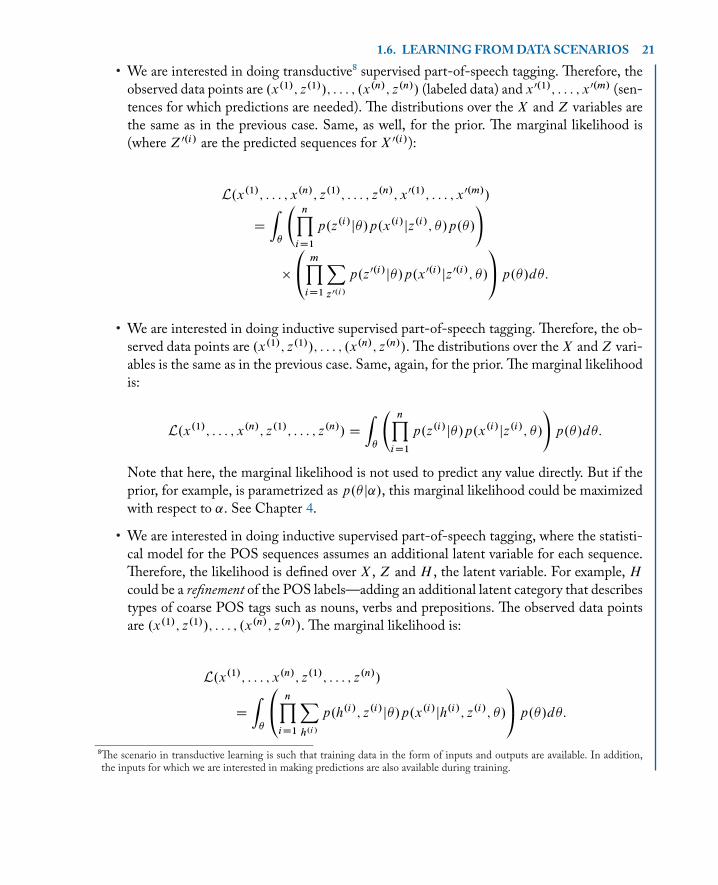
1.6. LEARNING FROM DATA SCENARIOS 21

• We are interested in doing transductive⁸ supervised part-of-speech tagging. erefore, theobserved data points are .x.1/; z.1//; : : : ; .x.n/; z.n// (labeled data) and x0.1/; : : : ; x0.m/ (sen-tences for which predictions are needed). e distributions over the X and Z variables arethe same as in the previous case. Same, as well, for the prior. e marginal likelihood is(where Z0.i/ are the predicted sequences for X 0.i/):

L.x.1/; : : : ; x.n/; z.1/; : : : ; z.n/; x0.1/; : : : ; x0.m//

D

Z�

nYiD1

p.z.i/j�/p.x.i/jz.i/; �/p.�/

!

�

0@ mYiD1

Xz0.i/

p.z0.i/j�/p.x0.i/

jz0.i/; �/

1Ap.�/d�:• We are interested in doing inductive supervised part-of-speech tagging. erefore, the ob-

served data points are .x.1/; z.1//; : : : ; .x.n/; z.n//. e distributions over the X and Z vari-ables is the same as in the previous case. Same, again, for the prior. e marginal likelihoodis:

L.x.1/; : : : ; x.n/; z.1/; : : : ; z.n// DZ�

nYiD1

p.z.i/j�/p.x.i/jz.i/; �/

!p.�/d�:

Note that here, the marginal likelihood is not used to predict any value directly. But if theprior, for example, is parametrized as p.� j˛/, this marginal likelihood could be maximizedwith respect to ˛. See Chapter 4.

• We are interested in doing inductive supervised part-of-speech tagging, where the statisti-cal model for the POS sequences assumes an additional latent variable for each sequence.erefore, the likelihood is defined over X , Z and H , the latent variable. For example, Hcould be a refinement of the POS labels—adding an additional latent category that describestypes of coarse POS tags such as nouns, verbs and prepositions. e observed data pointsare .x.1/; z.1//; : : : ; .x.n/; z.n//. e marginal likelihood is:

L.x.1/; : : : ; x.n/; z.1/; : : : ; z.n//

D

Z�

0@ nYiD1

Xh.i/

p.h.i/; z.i/j�/p.x.i/jh.i/; z.i/; �/

1Ap.�/d�:⁸e scenario in transductive learning is such that training data in the form of inputs and outputs are available. In addition,the inputs for which we are interested in making predictions are also available during training.

22 1. PRELIMINARIES

e concept of likelihood is further explored in this book in various contexts, most promi-nently in Chapters 4 and 6.

Log-likelihood and marginal log-likelihood can also be used as an “intrinsic” measure ofevaluation for a given model. is evaluation is done by holding out part of the observed data,and then evaluating the marginal log-likelihood on this held-out dataset. e higher this log-likelihood is for a given model, the better “fit” it has to the data.

e reason for doing this kind of evaluation on a held-out dataset is to ensure that the gen-eralization power of the model is the parameter being tested. Otherwise, if we were to evaluate thelog-likelihood on the observed data during learning and initial inference, we could always createa dummy, not-so-useful model that would give higher log-likelihood than any other model. isdummy model would be created by defining a probability distribution (unconstrained to a specificmodel family) which assigns probability 1=n to each instance in the observed data. Such distribu-tion, however, would not generalize well for complex sample spaces. Still, evaluation of marginallog-likelihood on the training data could be used for other purposes, such as hyperparametertuning.

1.7 BAYESIAN AND FREQUENTIST PHILOSOPHY (TIP OFTHE ICEBERG)

e main difference between the Bayesian approach and the frequentist approach is the interpre-tation of the concept of “probability.” e frequentist view, as its name implies, views probability(of an event) as a number that denotes its “relative frequency” in a large number of repeatedidentical experiments. e Bayesian view, on the other hand, views probability as a number thatdenotes our state of knowledge about the event. Within the supporters of Bayesian statistics,there are two camps. ose who view Bayesian probability as an objective, rational measure of thestate of knowledge (objectivists), and those who view it as as indication of personal belief (sub-jectivists). is means that objectivists advocate a rather uniform inference from data betweenmodelers who share the same knowledge about the problem, while subjectivists advocate that thisinference may differ and highly depend on personal beliefs.

Both subjectivists and objectivists perform inference by applying Bayes’ rule, and invertingthe relationship between the data and the hypotheses or the model. Objectivists, however, wantto minimize the influence that a person has on the inference process, so that the final conclusionsare determined, as much as possible, based on the data. e attempt to minimize this influenceis sometimes done by introducing “reference” or non-informative priors, such as Jeffreys prior(Section 3.3.2).

In science, the frequentist approach is associated with the hypothetico-deductive approach.is means that a hypothesis is formed, tested and finally accepted or rejected. e frequentistapproach is based on the idea of falsification of a theory, and is conducted through statisticaltests, hypothesis testing and other methods which support this idea. e Bayesian approach, on

1.8. SUMMARY 23

the other hand, is more typically associated with inductive inference. Data is collected, and thenwe make an update to our beliefs about the theory at hand. Some might argue that the Bayesianapproach can also be thought of as hypothetico-deductive (see for example Gelman and Shalizi(2013)). For a discussion of the Bayesian and frequentist philosophy, see Jaynes (2003).

1.8 SUMMARYIn this chapter we described the fundamental concepts for Probability and Statistics required forunderstanding this book. Some of the concepts we described include:

• Probability measures, probability distributions and sample spaces.

• Random variables (which are functions over the sample space).

• Joint probability distributions (which define a probability distribution over several randomvariables) and conditional probability distributions (which define a probability distributionover a set of random variables, while permitting clamping for the values of others).

• Independence between random variables (which implies that two sets of random variablesare not informative about one another) and conditional independence between random vari-ables (which implies that two sets of random variables are not informative about one anotherassuming we know the value of a third set of random variables).

• Bayes’ rule and the chain rule.

• Expectations (which compute the mean of a function, weighted against a probability dis-tribution).

• Models (which are sets of probability distributions).

• Estimation (identifying a specific member of a model family based on data; most commonlyused in the frequentist setting).

• Bayesian statistical inference (which requires the use of Bayes’ rule to compute a probabilitydistribution, the posterior, over the parameter space, given observed data).

24 1. PRELIMINARIES

1.9 EXERCISES1.1. Let p be a probability measure over� andA, B and C three events (subsets of�). Using

the axioms of probability measures, prove that

p.A [ B [ C/

D p.A/C p.B/C p.C / � p.A \ B/ � p.A \ C/ � p.B \ C/C p.A \ B \ C/:

(is formula can be generalized to an arbitrary number of events, based on the inclusion-exclusion principle.)

1.2. Let� be the set of natural numbers. Can you define a probability measure p over� suchthat p.x/ D p.y/ for any x; y 2 �? If not, show that such measure does not exist.

1.3. Describe the distribution of two random variables X and Y , such that X and Y areuncorrelated but not independent.

1.4. For a given n, describe n random variables such that any subset of them is independent,but all n random variables together are not.

1.5. Consider the graphical model in Figure 1.1 and its joint distribution in Equation 1.5.Fix j 2 f1; : : : ; N g. Using the definition of conditional independence, show thatW .j /

i isconditionally independent of W .j /

kfor k ¤ i given Z.j /i . In addition, show that Z.j /i is

conditionally independent of Z.k/`

for k ¤ j and any `, given � .j /. Is Z.j /i conditionallyindependent of Z.j /

`given � .j / for ` ¤ i?