Western UniversityScholarship@Western

Electronic Thesis and Dissertation Repository

June 2012

Bayesian Analyses of Metal-Loss Corrosion onEnergy Pipeline Based on Inspection DataMohammad Al-Amin

SupervisorDr. Wenxing ZhouThe University of Western Ontario

Graduate Program in Civil and Environmental Engineering

A thesis submitted in partial fulfillment of the requirements for the degree in Master of Engineering Science

© Mohammad Al-Amin 2012

Follow this and additional works at: https://ir.lib.uwo.ca/etd

Part of the Civil and Environmental Engineering Commons

This Dissertation/Thesis is brought to you for free and open access by Scholarship@Western. It has been accepted for inclusion in Electronic Thesisand Dissertation Repository by an authorized administrator of Scholarship@Western. For more information, please contact tadam@uwo.ca,wlswadmin@uwo.ca.

Recommended CitationAl-Amin, Mohammad, "Bayesian Analyses of Metal-Loss Corrosion on Energy Pipeline Based on Inspection Data" (2012). ElectronicThesis and Dissertation Repository. 588.https://ir.lib.uwo.ca/etd/588

BAYESIAN ANALYSES OF METAL-LOSS CORROSION ON

ENERGY PIPELINES BASED ON INSPECTION DATA

(Spine title: Bayesian Analyses of Metal-loss Corrosion on Energy Pipelines)

(Thesis format: Integrated Article)

by

Mohammad Al-Amin

Graduate Program in Engineering Science

Department of Civil and Environmental Engineering

A thesis submitted in partial fulfillment

of the requirements for the degree of

Master of Engineering Science

The School of Graduate and Postdoctoral Studies

Western University

London, Ontario, Canada

© Mohammad Al-Amin 2012

ii

WESTERN UNIVERSITY

SCHOOL OF GRADUATE AND POSTDOCTORAL STUDIES

CERTIFICATE OF EXAMINATION

Supervisor

______________________________

Dr. Wenxing Zhou

Supervisory Committee

______________________________

Dr. Hanping Hong

Examiners

______________________________

Dr. F. Michael Bartlett

______________________________

Dr. Hanping Hong

______________________________

Dr. Jeff T. Wood

The thesis by

Mohammad Al-Amin

entitled:

Bayesian analyses of Metal-loss Corrosion on Energy Pipelines Based on

Inspection Data

is accepted in partial fulfillment of the

requirements for the degree of

Master of Engineering Science

Date ______________________ _______________________________

Chair of the Thesis Examination Board

iii

Abstract

Bayesian models are developed to calibrate the accuracies of high-resolution in-line

inspection (ILI) tools for sizing metal-loss corrosion defects and to characterize the

growth of individual defects on energy pipelines. Moreover, a methodology is proposed

to evaluate the time-dependent system reliability of a segment of a pressurized pipeline

containing multiple active corrosion defects. The calibration of ILI tools is carried out by

comparing the field-measured depths and ILI-reported depths for a set of static defects.

The measurement error associated with the field-measuring tool is found to be negligibly

small; therefore, the field-measured depth is assumed to equal the actual depth of the

defect. The depth of a corrosion defect reported by an ILI tool is assumed to be a linear

function of the corresponding field-measured depth subjected to a random scattering

error. The probabilistic characteristics of the intercept and slope in the linear function,

i.e. the constant and non-constant biases of the measurement error, as well as the standard

deviation of the random scattering error are then quantified using the Bayesian

methodology. The proposed methodology is able to calibrate the accuracies of multiple

ILI tools simultaneously and quantify the potential correlations between the random

scattering errors associated with different ILI tools.

The corrosion growth model is developed in a hierarchical Bayesian framework. The

depth of the corrosion defects is assumed to be a power-law function of time

characterized by two power-law coefficients and the corrosion initiation time, and the

probabilistic characteristics of the parameters involved in the growth model are evaluated

using Markov Chain Monte Carlo (MCMC) simulation technique based on ILI data

iv

collected at different times for a given pipeline. The model accounts for the constant and

non-constant biases and random scattering errors of the ILI data, as well as the potential

correlation between the random scattering errors associated with different ILI tools. The

model is validated by comparing the predicted depths with the field-measured depths of

two sets of external corrosion defects identified on two in-service natural gas pipelines.

A simulation-based methodology is proposed to evaluate the time-dependent system

reliability of a segment of a pressurized pipeline containing multiple active metal-loss

corrosion defects. The methodology considers three distinctive failure modes, namely

small leak, large leak and rupture, and incorporates the hierarchical Bayesian power-law

growth model for the depth of individual corrosion defect. Both the conventional Monte

Carlo simulation and MCMC simulation techniques are employed in the methodology to

evaluate the failure probability. The methodology is illustrated using a joint of an

underground natural gas pipeline that is currently in service.

Keywords: Metal-loss corrosion, pipeline, ILI, growth model, measurement error,

Bayesian updating, MCMC and reliability.

v

Dedication

To my parents, Md. Moslem Miah and Safia Khatoon

vi

Acknowledgments

First of all, I would like to express my sincere appreciation and deep gratitude to my

supervisor, Dr. Wenxing Zhou for his patient guidance, understanding, and most

importantly for continuously supporting me with his profound insight, and constant

encouragement throughout this study. I was fortunate enough to have the opportunity of

being a member of his research group. His door was always open for me even in his

busiest days. This thesis would definitely have not been possible without him.

I would also like to thank Dr. Hanping Hong, Dr. Michael Bartlett and Dr. Jeff T.

Wood for being my examiners and for their constructive advice to this thesis. I would

also express my gratitude to Shahani Kariyawasam and Hong Wang from TransCanada

for their valuable comments and suggestions during a project related to my thesis.

I would like to thank my colleagues of our research group for making my graduate

life so enjoyable and also for their encouragement and assistances. My especial thanks

go to Shenwei Zhang who helped me a lot not only in my research but also the courses

we took together.

Financial support provided by TransCanada and the Natural Sciences and

Engineering Research Council of Canada (NSERC) and by the Faculty of Engineering at

Western University is gratefully acknowledged.

Finally, I would like to thank my parents and my sisters for everything they have

done for me leading up to this moment. Last but not least, I would like to thank Jannatul

Fardows for her love, encouragement and support throughout my Master’s program.

vii

Table of Contents

CERTIFICATE OF EXAMINATION ........................................................................... ii

Abstract ............................................................................................................................. iii

Dedication .......................................................................................................................... v

Acknowledgments ............................................................................................................ vi

Table of Contents ............................................................................................................ vii

List of Tables ................................................................................................................... xii

List of Figures ................................................................................................................. xiii

List of Abbreviations, Symbols, Nomenclature ............................................................ xv

Chapter 1 Introduction .................................................................................................... 1

1.1 Background ............................................................................................................... 1

1.2 Objective and Research Significance ........................................................................ 8

1.3 Scope of the Study .................................................................................................... 8

1.4 Thesis Format .......................................................................................................... 10

References ..................................................................................................................... 10

Chapter 2 Bayesian Model for Calibration of ILI Tools ............................................ 13

2.1 Introduction ............................................................................................................. 13

2.2 Bayesian Methodology ........................................................................................... 16

2.2.1 Basic Formulation ............................................................................................ 16

viii

2.2.2 Markov Chain Monte Carlo Simulation .......................................................... 18

2.3 Measurement Error Model for Corrosion Defects .................................................. 20

2.4 Measurement Error of Field Measurement ............................................................. 22

2.5 Bayesian Calibration Model for ILI Tools .............................................................. 24

2.5.1 Formulation and the Likelihood Function ....................................................... 24

2.5.2 Prior Distributions ............................................................................................ 25

2.6 Case Study .............................................................................................................. 27

2.6.1 General ............................................................................................................. 27

2.6.2 Case 1 ............................................................................................................... 28

2.6.3 Case 2 ............................................................................................................... 38

2.7 Conclusion .............................................................................................................. 42

References ..................................................................................................................... 43

Chapter 3 Hierarchical Bayesian Corrosion Growth Model Based on In-Line

Inspection Data................................................................................................................ 46

3.1 Introduction ............................................................................................................. 46

3.2 Hierarchical Bayesian Model .................................................................................. 49

3.3 ILI Data and Measurement Uncertainties ............................................................... 54

3.4 Hierarchical Bayesian Corrosion Growth Model ................................................... 55

3.4.1 Formulation and the Likelihood Function ....................................................... 55

3.4.2 Prior Distribution ............................................................................................. 57

ix

3.4.3 Hyper-prior Distribution .................................................................................. 58

3.5 Case Study .............................................................................................................. 60

3.5.1 General ............................................................................................................. 60

3.5.2 Case 1 ............................................................................................................... 61

3.5.3 Case 2 ............................................................................................................... 77

3.5.4 Effect of Correlation among the Random Scattering Measurement Errors ..... 88

3.6 Comparison with Industry Practice ......................................................................... 93

3.7 Conclusion .............................................................................................................. 95

References ..................................................................................................................... 97

Chapter 4 Time-dependent System Reliability Analysis of a Corroding

Pipeline ......................................................................................................................... 101

4.1 Introduction ........................................................................................................... 101

4.2 Limit State Functions ............................................................................................ 104

4.3 Burst and Rupture Pressure Models ...................................................................... 107

4.4 Corrosion Growth Model ...................................................................................... 109

4.5 System Reliability Analysis ...................................................................................110

4.5.1 Basic Assumptions ..........................................................................................110

4.5.2 Analysis Procedure..........................................................................................110

4.6 Numerical Example ...............................................................................................113

4.6.1 General ............................................................................................................113

x

4.6.2 Growth Mode for the Defect Depth ................................................................114

4.6.3 Probabilistic Characteristics of Input Parameters ...........................................118

4.6.4 Results ............................................................................................................ 120

4.6.5 Sensitivity analysis......................................................................................... 121

4.7 Conclusion ............................................................................................................ 124

References ................................................................................................................... 125

Chapter 5 Summary and Conclusions ....................................................................... 128

5.1 General .................................................................................................................. 128

5.2 Bayesian Model for Calibration of ILI Tools ........................................................ 128

5.3 Hierarchical Bayesian Corrosion Growth Model Based on In-line

Inspection Data ........................................................................................................... 130

5.4 Time-dependent System Reliability Analysis of a Corroding Pipeline ................ 133

5.5 Recommendations for Future Work ...................................................................... 134

References ................................................................................................................... 135

Appendix 2A Algorithms for Performing Markov Chain Monte Carlo

Simulation ...................................................................................................................... 136

2A.1 Metropolis-Hastings Algorithm ......................................................................... 136

2A.2 Gibbs Sampler .................................................................................................... 139

References ................................................................................................................... 142

Appendix 2B Grubbs’ Estimator and Jaech’s Estimator ......................................... 144

xi

2B.1 Grubbs’ Estimator .............................................................................................. 144

2B.2 Jaech’s Estimator ................................................................................................ 145

References ................................................................................................................... 146

Appendix 2C Derivation of the Conditional Posterior Distributions of

Parameters of Bayesian Calibration Model ............................................................... 147

Appendix 2D OpenBUGS code for Bayesian calibration model of Case 1 ............. 152

Appendix 2E OpenBUGS code for Bayesian calibration model of Case 2 ............. 156

Appendix 3A Derivation of the Conditional Posterior Distributions of the

HBM corrosion growth model ..................................................................................... 160

Appendix 3B OpenBUGS code for HBM model of Case 1 ....................................... 166

Appendix 3C OpenBUGS code for HBM model of Case 2 ...................................... 171

Curriculum Vitae .......................................................................................................... 176

xii

List of Tables

Table 2.1 Mean values of the parameters in the calibration models for ILI

tools used in Case 1........................................................................................................... 35

Table 2.2 Mean values of the correlation coefficients (kl) between the

random scattering errors for different ILI tools used in Case 1 ........................................ 35

Table 2.3 Mean values of the parameters in the calibration models for

ILI tools used in Case 2 .................................................................................................... 39

Table 2.4 Mean values of the correlation coefficients (kl) between the

random scattering errors for different ILI tools in Case 2 ................................................ 40

Table 3.1 MSEP’s for the models with partially-correlated, fully-correlated and

independent random scattering errors ............................................................................... 90

Table 3.2 p-values of the null hypothesis, Ho: MSEP1 = MESP2 (MSEP1 = MESP3)

and alternative hypothesis Ha: MSEP1 < MESP2 (MSEP1 < MESP3) .............................. 92

Table 4.1 Probabilistic characteristics of the basic random variables used

in the reliability analysis ..................................................................................................119

Table 4.2 Nominal values of the input parameters used in the reliability analysis ......... 120

xiii

List of Figures

Figure 1.1 Schematic of a general corrosion process ......................................................... 3

Figure 1.2 Corrosion mechanism on an underground metallic pipeline (Beavers and

Thompson 2006) ................................................................................................................. 4

Figure 1.3 Example of corrosion on a steel pipeline .......................................................... 4

Figure 1.4 A typical in-line inspection tool ......................................................................... 6

Figure 1.5 Sensor configuration of an MFL tool (Clapham et al. 2004) ............................ 6

Figure 2.1 Comparison of defect depths measured by laser scan technology and UT ..... 23

Figure 2.2 Manual matching of defects on a selected pipe joint ...................................... 28

Figure 2.3 Trace plots of 1, 2, 3, and 4 ...................................................................... 30

Figure 2.4 Trace plots of 1, 2, 3, and 4 ....................................................................... 31

Figure 2.5 Trace plots of 11, 12 and 22 ...................................................................... 32

Figure 2.6 Marginal posterior distributions of 1, 2, 3, and 4 ..................................... 33

Figure 2.7 Marginal posterior distributions of 1, 2, 3, and 4 ...................................... 33

Figure 2.8 Comparison of field-measured depths and ILI-reported depths for

the recoated defects on the pipeline in Case 1 .................................................................. 38

Figure 2.9 Comparison of field-measured depths and ILI-reported depths for

the recoated defects on the pipeline in Case 2 .................................................................. 41

Figure 3.1 Graphical representation of a typical hierarchical Bayesian model ................ 52

Figure 3.2 Graphical representation of the full hierarchical Bayesian corrosion

growth model .................................................................................................................... 60

Figure 3.3 Apparent growth paths of the 62 corrosion defects indicated by

the ILI data ........................................................................................................................ 62

Figure 3.4 Trace plots of a1, a2 and a3 .............................................................................. 65

Figure 3.5 Trace plots of b1, b2 and b3 .............................................................................. 66

Figure 3.6 Trace plots of to1, to2 and to3 ............................................................................. 67

Figure 3.7 Box plot of the components of parameter vector a of Case 1 ......................... 69

Figure 3.8 Box plot of the components of parameter vector b of Case 1 ......................... 70

Figure 3.9 Box plot of the components of parameter vector to of Case 1 ......................... 71

Figure 3.10 Box plot of the components of parameter vector of Case 1 ..................... 72

Figure 3.11 Comparison between the predicted and field- measured depths

in 2010 for Case 1 ............................................................................................................. 74

xiv

Figure 3.12 Predicted growth paths for defects #3, #6, #7, #19 and #60

on pipeline of Case 1......................................................................................................... 77

Figure 3.13 Apparent growth paths of the 60 corrosion defects indicated

by the ILI data ................................................................................................................... 78

Figure 3.14 Box plot of the components of parameter vector a of Case 2 ....................... 80

Figure 3.15 Box plot of the components of parameter vector b of Case 2 ....................... 81

Figure 3.16 Box plot of the components of parameter vector to of Case 2 ....................... 82

Figure 3.17 Box plot of the components of parameter vector of Case 2 ..................... 83

Figure 3.18 Comparison between the predicted and field-measured depths

in 2011 for Case 2 ............................................................................................................. 84

Figure 3.19 Predicted growth paths for defect #13, #23, #35, #50 and #56

on pipeline of Case 2......................................................................................................... 87

Figure 3.20 Comparison of the predicted depths from the models with partially-

correlated, fully-correlated and independent random scattering errors with

field-measured depths in 2010 for the corrosion defects in Case 1 .................................. 89

Figure 3.21 Comparison of the predicted depths from the models with partially-

correlated, fully-correlated and independent random scattering errors with

field-measured depths in 2011 for the corrosion defects in Case 2 .................................. 89

Figure 3.22 Comparison between the predicted depths from the linear growth

model and field-measured depths in 2010 for the corrosion defects in Case 1 ................ 94

Figure 3.23 Comparison between the predicted depths from the linear growth

model and field-measured depths in 2011 for the corrosion defects in Case 2 ................ 95

Figure 4.1 Dimensions of a typical corrosion defect on pipeline ................................... 105

Figure 4.2 Predicted growth paths for defects #2, #4, #5 and #7 on the selected

pipe joint ..........................................................................................................................116

Figure 4.3 Marginal posterior probability density functions of predicted depths

in 2012, 2016 and 2021 for defects #2, #4, #5 and #7 .....................................................118

Figure 4.4 Cumulative failure probabilities of the pipe segment for three different

failure modes ................................................................................................................... 121

Figure 4.5 Impact of correlation between the model errors of the burst capacity

models, e, for different defects on the system reliability ................................................ 122

Figure 4.6 Impact of correlation between the maximum-to-average depth

ratios, , for different defects on the system reliability .................................................. 123

xv

List of Abbreviations, Symbols, Nomenclature

ai, bi = parameters of the power-law growth model for defect i

D = outside diameter of the pipeline

dai = actual depth of the ith

static defect

daij = actual depth of the ith

defect at the time of the jth

inspection

davg = average depth of the corrosion defect

dfi = field-measured depth of the ith

static defect

dfij = field-measured depth of the ith

defect at the time of the jth

inspection

dmax = maximum depth of the corrosion defect

dmij = ILI-reported depth of the ith

defect obtained from the jth

inspection

e = model error associated with the burst capacity model

g1 = limit state function for the corrosion defect penetrating the pipe wall

g2 = limit state function for plastic collapse under internal pressure at the defect

g3 = limit state function for the unstable axial extension of the through-wall

Ha = alternative hypothesis

Ho = null hypothesis

HBM = hierarchical Bayesian model

ILI = in-line inspection

iid = independent and identically distributed

ind = independent

li = length of corrosion defect i

loi = length of the defect i at the time of last inspection

rl = length growth rate of corrosion defect

MCMC = Markov chain Monte Carlo

MFL = Magnetic Flux Leakage

MSEP = mean squared error of prediction

M = Folias factor or bulging factor

Pll = probability of large leak

Prp = probability of rupture

xvi

Psl = probability of small leak

p = internal pressure of the pipeline

rb = burst pressure resistance of the pipe at the defect

rbc = predicted burst pressure without model error

ri = growth rate for defect i in the linear model

ro = burst pressure resistance of a defect-free pipe

rrp = pressure resistance of the pipeline at the location of the through-wall defect

SMYS = specified minimum yield stress

SMTS = specified minimum tensile strength

T = total forecasting period

toi = corrosion initiation time of defect i

tj = elapsed time from the installation date up to the jth

inspection

UT = ultrasonic

wt = wall thickness

j = constant bias associated with jth

inspection tool

j = non-constant bias associated with jth

inspection tool

i = vector of random scattering errors associated with the depths reported by ILI

tools for the ith

defect

ij = random scattering errors of the ILI-reported depths of the ith

defect at the jth

inspection

i = random scattering errors of the field-measured depth of the ith

static defect

ij = random scattering errors of the field-measured depth of the ith

defect at the jth

inspection

ij = model error of the power-law growth model associated with defect i at time j

a = mean value of the prior distribution of ai

b = mean value of the prior distribution of bi

μi = vector of mean values of ILI-reported depths at different times for defect i

= covariance matrix of random scattering error

a2 = variance of the prior distribution of ai

b2 = variance of the prior distribution of bi

xvii

f = flow stress of the pipe steel

k = standard deviation of the random scattering error of the ILI tool used in the

kth

inspection

y = yield strength of the pipe steel

u = ultimate strength of the pipe steel

k2 = variance of the random scattering error of the ILI tool used in the k

th

inspection

i2 = variance of the prior distribution of ij associated with defect i

kl = correlation coefficient between the random scattering errors associated with

the ILI tools used in the kth

and lth

inspections

= time elapsed between the year of last inspection and the year for which the

failure probability is forecasted

= maximum-to-average depth ratio for corrosion defects on pipeline

1

Chapter 1 Introduction

1.1 Background

Pipelines are transport large quantities of hydrocarbons (e.g. crude oil and natural

gas) from the production sites to the end users. Compared with other means of

transporting hydrocarbons such as rail cars and tanker trucks, pipelines are safer, more

efficient and cost-effective (PHMSA 2012). There are about 500,000 km of transmission

pipelines that carry natural gas, oil, and other hazardous liquids across the United States

(Parfomak 2011). According to the Canadian Energy Pipeline Association, there are

more than 100,000 km of oil and gas transmission pipelines in Canada. In 2010, the

71,000 km long pipelines regulated by the National Energy Board (NEB) of Canada

shipped about $85.5 billion worth of hydrocarbons at an estimated transportation cost of

only $5.5 billion ( NEB 2010).

As pipelines age the protective coatings on the pipelines have the potential to lose

their effectiveness and therefore leave the pipelines vulnerable to corrosion (Benmoussa

et al. 2006; Jeglic 2004). In fact, corrosion is one of the most common contributors to the

failure of transmission pipelines in North America and Western Europe (Bolt and Owen

1999; Eiber et al. 1995; PHMSA 2012). A comparative study of pipeline performance

reported by NEB (2008) indicates that about 63% of pipeline ruptures (the most severe

pipeline failure mode) that had occurred between 1991 and 2006 on the NEB-regulated

pipelines in Canada were due to corrosion (metal loss and stress corrosion cracking, as

defined by CSA Z662-07). The data collected by the Pipeline and Hazardous Materials

2

Safety Administration (PHMSA) of the United States Department of Transportation

(DOT) show that approximately 25% of pipeline ruptures were caused by corrosion

during this time span in the US. The PHMSA database (PHMSA 2012) indicates that

corrosion was the cause for a total of 166 significant incidents1 on the onshore gas

pipelines in the US between 1992 and 2011; these incidents resulted in 13 fatalities, 4

injuries and a total property loss of worth about $115 million (in 2011 US $).

Corrosion is an electro-chemical process that is caused by the chemical interaction

between metal and its surrounding environment, and results in degradation of metal

(Davis 2000; Peabody 2001). The corrosion process involves the combination of

oxidation and reduction reactions, referred to as the Redox reaction. The coupled action

of losing electrons (oxidation) by the metal and consuming those electrons (reduction) by

the oxidant such as oxygen is key for corrosion to occur. The typical oxidation and

reduction reactions for steel are shown in Eqs. (1.1) and (1.2), respectively.

(1.1)

(1.2)

1 A significant incident is defined by DOT as an incident that causes one or more of the following: 1)

fatalities or injuries requiring hospitalization the patient; 2) property damage exceeding a certain monetary

threshold; 3) product loss exceeding a certain amount and 4) release of product resulting in fire or

explosion.

3

The mechanism of general corrosion is schematically shown in Fig. 1.1. As shown in

the figure, the essential conditions for corrosion to take place are 1) existence of an anode

and a cathode; 2) metallic connection between the anode and cathode (i.e. the electrode),

and 3) immersion of anode and cathode in an electrically conducive medium (i.e. the

electrolyte). The anode, cathode, electrode and electrolyte are all contained in the so-

called corrosion cell.

Figure 1.1 Schematic of a general corrosion process

In case of underground pipelines, the anode and cathode in the corrosion cell can

form at different locations on the same pipeline due to the differences in metal grain

composition, milling imperfections, scratches, threads, etc (Beavers and Thompson

2006). The pipeline itself acts as the electrode, whereas the surrounding soil works as the

electrolyte. The difference in the soil resistivity, oxygen concentration, moisture content

2e-anode cathode

electrolyte

Fe++

electrode

4

and various ion concentrations favors the flow of free electrons. Once corrosion starts to

occur, the anode portion of the pipe will corrode, resulting in metal loss and thinning of

the pipe wall. The mechanism of corrosion on a pipeline is illustrated in Fig. 1.2. An

entire corrosion cell can occur within a drop of water. Therefore, hundreds of corrosion

defects can appear within a small portion of a pipeline. Figure 1.3 shows corrosion on an

underground steel pipeline.

Figure 1.2 Corrosion mechanism on an underground metallic pipeline (Beavers and

Thompson 2006)

Figure 1.3 Example of corrosion on a steel pipeline

anode cathode

e-

Oxygen-rich soilOxygen-deficient soil

5

In-line inspection (ILI) tools, also known as “smart pigs”, are widely used to detect,

locate and size corrosion anomalies on pipelines (Caleyo et al. 2007; Desjardins 2001;

Nessim et al. 2008). There are mainly two types of ILI tools, namely the magnetic flux

leakage (MFL) and ultrasonic (UT) tools. The MFL tools are commonly used to inspect

gas pipelines, whereas UT tools are used in liquid pipelines. A typical high resolution

MFL tool is shown in Fig. 1.4. Because the inspection data available to this study all

come from MFL tools, the underlying mechanisms of the MFL tool are briefly described

in the following.

During an in-line inspection, an MFL tool is propelled by the product in the pipeline

and produces a magnetic flux in the pipe wall using a strong permanent magnet or direct

current electromagnet. The presence of a corrosion defect causes the distortion of the

flux field, i.e. the so-called leakage, which is detected by the circumferential array of the

MFL detectors. Once a defect is identified, the leakage signal and position (longitudinal

and circumferential) of the signal on the pipeline are recorded and stored in the data

recording device of the tool. High-resolution MFL tools (commonly used nowadays) can

differentiate between corrosion defects located on the external and internal surfaces of the

pipe wall. The mechanism of detecting a corrosion defects on pipeline by a typical MFL

tool is depicted in Fig. 1.5, which is reproduced from Clapham et al. (2004).

6

Figure 1.4 A typical in-line inspection tool

Figure 1.5 Sensor configuration of an MFL tool (Clapham et al. 2004)

The leakage signal obtained from the ILI tool represents the volumetric metal loss of

the pipe wall. These signals are then converted into the defect geometry, i.e. depth (in the

through pipe wall thickness direction), length (in the pipeline’s longitudinal direction)

and width (in the pipeline’s circumferential direction), using the sizing algorithm of that

particular tool. The sizing algorithm is usually developed based on the so-called pull

through test (Race et al. 2007; Sutherland et al. 2010), where a section of pipeline with

pre-generated defects of several depth, length and width ranges are tested by the ILI tool.

SensorMount

Back Iron Mounting Plate

Motion

PitPipe Wall

Magnet Magnet

Steel

Brushes

Steel

Brushes

Leakage

Flux

7

The signals obtained from the tool are calibrated against the known depths, lengths and

widths of the defects to develop a sizing model. From the results of the pull through test,

ILI vendors can also quantify the tool accuracy. The accuracy of an ILI tool is

commonly specified as a two-sided confidence interval, e.g. the measured defect depth is

accurate within ±10% wall thickness (wt) with a confidence level of 80%.

Pipeline operators develop and implement comprehensive integrity management

programs to ensure the safe operation of pipelines. The pipeline integrity management

with respect to corrosion typically consists of in-line inspection, defect assessment and

mitigation (Kishawy and Gabbar 2010). Characterization of the growth of corrosion

defects plays a crucial role in the pipeline integrity management. The corrosion growth

rate is essential to the forecast of the failure probability of the pipelines, determination of

the inspection interval and prioritization of defect mitigation and repair. On one hand,

overly conservative estimates of the corrosion growth rates lead to too frequent

inspections and unnecessary excavations and repairs, making the integrity management

program costly. On the other hand, under-estimation of the corrosion growth may leave

critical defects unmitigated and result in failure of the pipeline.

As more and more pipelines are now being inspected by ILI tools on a regular basis,

the ILI data from multiple inspections naturally provide valuable information about the

growth of corrosion defects on the pipeline. Therefore, there is a pressing need in the

pipeline industry for developing models to predict the growth of corrosion defects based

on repeated in-line inspections data (Kariyawasam and Peterson 2010). This is the main

drive for the present study.

8

1.2 Objective and Research Significance

The study reported in this thesis is a part of a Collaborative Research and

Development (CRD) program jointly funded by the Natural Sciences and Engineering

Research Council (NSERC) of Canada and TransCanada Pipelines Limited. The

objectives of the study were 1) to develop a probabilistic model to characterize the

growth of the depths of individual metal-loss corrosion defects on energy pipelines based

on data collected from multiple ILIs; and 2) to incorporate the developed corrosion

growth model in the reliability analysis to evaluate the failure probability of the pipeline

due to corrosion. The study was focused on the growth of the depth of metal-loss

corrosion defects; the growth of length of metal-loss corrosion defects or growth of other

types of corrosion defects (e.g. stress corrosion cracking) was not considered.

The growth model developed in this study accounts for both systematic and random

measurement errors associated with ILI tools, and is specific to individual corrosion

defects. The model will assist pipeline integrity engineers in making informed decisions

about re-inspection interval and defect mitigation plan that satisfy both the safety and

resource constraints. The proposed reliability analysis method provides a framework to

incorporate the growth model in the pipeline corrosion reliability analysis, which will

facilitate reliability- and risk- based pipeline integrity management.

1.3 Scope of the Study

This study consists of three main components that are presented in Chapters 2, 3 and

4, respectively. Chapter 2 describes a Bayesian model to calibrate the ILI tools, i.e.

quantifying the measurement errors of the ILI tool, based on ILI-reported and field-

9

measured depths for the static defects on the pipeline. The application of the proposed

model was demonstrated using the static defects on two subject pipelines currently in

service in Alberta.

In Chapter 3, a hierarchical Bayesian corrosion growth model is presented to

characterize the growth of the depth of individual corrosion defects based on ILI data

from multiple inspections. This model takes into account the measurement errors (i.e.

bias and random scattering error) associated with the ILI tools and also the potential

correlation between the random scattering errors among different ILI tools. The Markov

Chain Monte Carlo (MCMC) simulation technique was employed to evaluate the

posterior distributions of the parameters of the growth model. Two sets of active

corrosion defects detected on the two subject pipelines considered in Chapter 2 were used

to illustrate and validate the proposed growth model.

Chapter 4 presents a methodology that can be used to evaluate the time-dependent

system reliability of a segment of onshore natural gas pipeline containing active corrosion

defects considering three distinctive failure modes, namely small leak, large leak and

rupture. The hierarchical corrosion growth model described in Chapter 3 was

incorporated in the reliability analysis to predict the depth of the corrosion defect at a

given time. The failure probability is evaluated using random samples generated from

both the simple Monte Carlo simulation and MCMC simulation. The methodology is

illustrated using a pipe joint in one of the subject pipelines.

10

1.4 Thesis Format

This thesis is prepared in an Integrated-Article Format as specified by the School of

Graduate and Postdoctoral Studies at Western University, Canada. The first chapter,

Chapter 1, is the introductory section of the entire thesis with its own bibliography. The

main body of the thesis contains three chapters, Chapters 2, 3 and 4. Each of these

chapters is presented as a stand-alone manuscript without any abstract, but with its own

references. The final chapter, Chapter 5, includes a summary of the study, main

conclusion of the thesis and recommendations for future work.

The tabulated data, mathematical derivations and programming codes are provided in

the appendices following the last chapter. An identification that consists of a number and

a letter is given to each appendix. The identification number and letter of each appendix

represent the associated chapter and the sequence of appearance of the appendix in that

chapter, respectively. For instance, Appendix 2A is the first appendix associated with

Chapter 2.

References

Beavers, J. A., and Thompson, N. G., 2006. External Corrosion of Oil and Natural

Gas Pipelines, ASM Handbook Volume 13C: Corrosion: Environments and Industries,

ASM International, pp. 1015-1025.

Benmoussa, A., Hadjel, M., and Traisnel, M., 2006. Corrosion behavior of API 5L X-

60 pipeline steel exposed to near-neutral pH soil simulating solution. Materials and

Corrosion, 57(10), pp. 771-777.

Bolt, R., and Owen, R. W., 1999. Recent Trends in Gas Pipeline Incidents (1970-

1997): a report by the European Gas Pipeline Incidents Data Group (EGIG), IMechE

Conference Transactions 1999-8 (C571), Institution of Mechanical Engineers, Newcastle

upon Tyne, UK.

11

Caleyo, F., Alfonso, L., Espina-Hernández, J. H., and Hallen, J. M., 2007. Criteria for

performance assessment and calibration of in-line inspections of oil and gas pipelines.

Measurement Science and Technology, 18(7).

Clapham, L., Babbar, V., and Byrne, J., 2004. Detection of Mechanical Damage using

the Magnetic Flux Leakage Technique. Proceedings of International Pipeline

Conference, ASME, Calgary, Alberta, Canada.

CSA, 2007. CSA-Z662 Oil and Gas Pipeline Systems. Canadian Standards

Associations, Rexdale, Ontario.

Davis, J. R., 2000. Corrosion: Understanding the Basics, ASM International, Ohio,

USA.

Desjardins, G., 2001. Corrosion Rate and Severity Results from In-Line Inspection

Data. CORROSION 2001, NACE International.

Eiber, R. J., Miele, C. R., and Wilson, P. R., 1995. An Analysis of DOT Reportable

Incidents on Gas Transmission and Gathering Lines for June 1984 Through 1992,

Topical Report to Line Pipe Research Supervisory Committee of the Pipeline Research

Committee of the American Gas Association, NG-18 Report No. 213, American Gas

Association.

Jeglic, F., 2004. Analysis of Ruptures and Trends on Major Canadian Pipeline

Systems, National Energy Board, Calgary, Canada.

Kariyawasam, S., and Peterson, W., 2010. Effective Improvements to Reliability

Based Corrosion Management. Proceedings of 8th International Pipeline Conference,

ASME, Calgary, Alberta, Canada, pp. 603-615.

Kishawy, H., and Gabbar, H., 2010. Review of Pipeline Integrity Management

Practices. International Journal of Pressure Vessels and Piping, 87 (7), pp. 373-380.

National Energy Board (NEB), 2008, Focus on Safety and Environment: A

Comparative Analysis of Pipeline Performance 2000–2006, National Energy Board,

Calgary, Alberta, Canada.

National Energy Board (NEB), 2010. Annual Report 2010 to Parliament, National

Energy Board, Canada.

Nessim, M., Dawson, J., Mora, R., and Hassanein, S., 2008. Obtaining Corrosion

Growth Rates From Repeat In-Line Inspection Runs and Dealing With the Measurement

Uncertainties. Proceedings of 7th International Pipeline Conference, ASME, Calgary,

Alberta, Canada, pp. 593-600.

Parfomak, P. W., 2011, Keeping America’s Pipelines Safe and Secure: Key Issues for

Congress, Encyclopedia of Earth.

12

Peabody, A. W., 2001. Control of Pipeline Corrosion. NACE International, Houston,

Texas, USA.

PHMSA, 2012, Pipeline Incidents and Mileage Reports, March 2012. Pipeline &

Hazardous Materials Safety Administration, http://primis.phmsa.dot.gov/comm/

reports/safety/PSI.html.

Race, J. M., Dawson, S. J., Stanley, L. M., and Kariyasawam, S., 2007. Development

of a predictive model for pipeline external corrosion rates. Journal of Pipeline

Engineering, 6(1), pp. 15-29.

Sutherland, J., Bluck, M., Pearce, J., and Quick, E., 2010. Validation of Latest

Generation MFL In-Line Inspection Technology Leads to Improved Detection and Sizing

Specification for Pinholes, Pitting, Axial Grooving and Axial Slotting. Proceedings of 8th

International Pipeline Conference, ASME, Calgary, Alberta, Canada, pp. 225-232.

13

Chapter 2 Bayesian Model for Calibration of ILI Tools

2.1 Introduction

Over the last few decades, the in-line inspection (ILI) technology has been widely

used to identify, locate and size corrosion defects on pipelines. Despite the enormous

advancement in the ILI technology, ILI data are subjected to measurement errors

resulting from imperfections in the ILI tool and associated sizing algorithm (Fenyvesi and

Dumalski 2005; Nessim et al. 2008). The measurement error includes the systematic

error, i.e. the constant and non-constant bias of the ILI data (Caleyo et al. 2007), and

random scattering error (i.e. repeatability error) of the data (Coleman and Miller 2010;

Spencer et al. 2010). Moreover, the corrosion growth rate calculated from multiple ILI

runs involve additional measurement errors due to differences in the magnetic strength of

different ILI tools, change of the defect sizing algorithm and differences in the sizing

model for defects, i.e. box or cluster, between inspections (Fenyvesi and Dumalski 2005).

The in-line inspection data can be used to quantify the growths of the depths of

corrosion defects on pipelines, which is considered one of the most critical tasks for

pipeline corrosion management. It is critically important to account for the measurement

error of the ILI data in determining the corrosion growth rate on pipelines (Bhatia et al.

1998). Although the measurement error can be inferred from the specifications of the ILI

tool, it is more appropriate to evaluate the de-facto measurement error of the ILI data for

a specific pipeline. Such an analysis is referred to as calibration of the ILI tool.

Knowledge of the de-facto measurement error will also help the ILI vendors to improve

14

the measurement technology and sizing algorithm for corrosion defects on a given

pipeline.

The measurement errors of the ILI data reported by a given ILI tool are typically

evaluated by comparing the field-measured and ILI-reported depths for a set of corrosion

defects. The field-measured depths are obtained from the dig sites using field-measuring

instruments, such as the pit gauge, ultrasonic thickness (UT) measuring device and the

laser profilometer. Bhatia et al. (1998) used the well-established Grubbs (Grubbs 1948)

and Jaech (Jaech 1985) estimators to quantify the measurement errors associated with the

ILI tool and the field-measuring instrument, and found that Grubbs’ method sometimes

result in negative values for the variance of the measurement error, which is unrealistic.

Jaech’s method can overcome such a drawback in Grubbs’ method and ensures that the

variance of the measurement error to be positive. Furthermore, both Grubbs’ method and

Jaech’s method assume that the measurement is unbiased; that is, the measurement error

only includes the random scattering error. This assumption may be unrealistic for ILI

tools.

Caleyo et al. (2007) developed a statistical method to calibrate the ILI tools using the

ILI-reported data and corresponding field measurements. The so-called V-Wald and V-

Jaech methods were introduced to quantify the bias of the ILI data and variances of the

scattering errors of both the ILI data and field measurements, respectively. However, the

potential correlations between the measurement errors associated with different ILI tools

that are based on the same inspection technology (e.g. MFL) and used to inspect the same

pipeline at different times cannot be evaluated from their reported model.

15

The objective of the study reported in this chapter was to develop a model to calibrate

the ILI tool and quantify the measurement error, including the constant and non-constant

bias as well as the random scattering error, of the ILI data. The potential correlations

between the scattering errors associated with different ILI tools were also considered in

the proposed model. The calibration was carried out using the Bayesian methodology

based on comparing the ILI data with the corresponding field measurements.

This chapter is organized as follows. Section 2.2 describes the statistical

methodologies (i.e. Bayesian method and Markov Chain Monte Carlo simulation)

employed in this study to calibrate the ILI tools. The basic assumptions associated with

the calibration model are presented in Section 2.3. Section 2.4 describes the

measurement errors associated with the field-measuring devices. Section 2.5 includes the

Bayesian formulation of the calibration model as well as the prior distributions for the

parameters of the calibration model. Section 2.6 illustrates the application of the

calibration model in two case studies that involve real ILI and field measurement data on

two pipelines currently in service. The conclusions of the chapter are summarized in

Section 2.7.

16

2.2 Bayesian Methodology

2.2.1 Basic Formulation

The Bayesian approach is an advanced tool to fit a probability model to a set of

observations by evaluating the unknown parameters of the model in a probabilistic way

(Gelman 2004). The Bayesian method treats the unknown parameters of a physical

process as random variables rather than as deterministic values. It incorporates the prior

knowledge about the parameters, which may arise from the results of previous studies or

experience. The prior knowledge is then updated based on the observed data to obtain

the revised opinion about the parameters. The updated belief can be further considered as

the prior distribution for future updating when new data are available. Therefore through

this iterative process the uncertainty in the parameters is minimized.

Given a set of n observations, X = (x1, x2, …, xn), and a collection of k unknown

parameters, θk) that characterize the physical process underlying the

observed data, one can specify the Bayesian model for the parameters. The objective of

the Bayesian analysis is to find the updated opinion about the unknown parameters θ

based on Bayes’ theorem given by (Bayes and Price 1763)

(2.1)

where p() denotes the probability density function of . Here p(θ),which is called the

prior distribution of the parameters, characterizes the belief regarding the unknown

parameters θ prior to any modeling. The information contained in the data is introduced

via the so-called likelihood for the data, p(X|θ), which is the value of the probability

17

density function associated with the data conditional on the parameters θ. The entity

p(θ|X) is known as the posterior distribution, which reflects the combined information

from the data and prior distribution. The quantity p(X) is a normalizing constant that

ensures the left hand side of Eq. (2.1) to be a probability distribution; that is, p(θ|X)

integrates to unity, and p(X) is known as the marginal likelihood and can be obtained by

integrating the numerator on the right hand side of Eq. (2.1) with respect to the unknown

parameters θ. Thus,

(2.2)

Taking into consideration the normalizing constant, one can write Eq. (2.1) as

(2.3)

where the symbol “ ” indicates proportionality.

Consider an example to illustrate the Bayesian method. Assume that y = (y1, y2, …,

yn) represents a set of n data that follow a Poisson distribution with an unknown rate

parameter . Further assume that the prior distribution of follows a gamma distribution

with known shape parameter and scale parameter . Therefore, the likelihood and prior

distribution can be written as,

ikelihood

Prior distribution:

18

where () denotes the gamma function.

The posterior distribution of can be evaluated from Eq. (2.3) as follows:

(2.4)

where

is the mean value of the observations. Note that the terms that are

independent of (such as Γ() and ) in Eq. (2.4) are omitted in the last step because

they are part of the proportionality constant. Based on Eq. (2.4), it can be concluded that

the posterior distribution of follows a gamma distribution with shape parameter and

scale parameters equal to n + and n+, respectively.

2.2.2 Markov Chain Monte Carlo Simulation

The main purpose of the Bayesian analysis is to evaluate the probabilistic

characteristics (e.g. mean, variance and quantiles) of the posterior distribution of the

unknown model parameters. Therefore, it is necessary to obtain the marginal posterior

distribution of each parameter. The marginal distribution of a parameter i of the

parameter vector , p(i|X), and the mean value of i, E(i|X), can be evaluated as

follows:

(2.5)

(2.6)

where (-i) denotes the vector of ’s excluding i.

19

In some cases, closed-form solutions of the integrals in Eqs. (2.5) and (2.6) are

available, or they can be easily computed using numerical methods. But in most

applications analytic or direct numerical evaluation of these integrals is very difficult, if

not impossible, due to the complexity and high dimensionality of the Bayesian model. To

overcome this difficulty, the Markov Chain Monte Carlo (MCMC) simulation technique

has been widely used in the Bayesian analysis (Gilks et al. 1996).

MCMC works by sequentially generating random samples of uncertain parameters to

form a Markov process whose stationary distribution is the joint posterior distribution of

the parameters. The difference between MCMC and the conventional Monte Carlo

simulation is that the sample generated in a given sequence in MCMC depends on the

sample generated in the previous sequence, whereas the samples generated in different

trials of the conventional Monte Carlo simulation are independent.

The MCMC simulation starts by assigning an arbitrary initial value to each of the

parameters considered. After an initial set of sequences, i.e. the so-called burn-in period,

the subsequent sequences are considered to converge to the joint posterior distribution of

the parameters. The samples generated in different sequences in MCMC are typically

autocorrelated. To reduce the autocorrelation, the so-called “thinning” technique is

employed, where only samples from every kth

(k > 1) iteration are stored for the output

analysis (Congdon 2006; Link and Eaton 2012). The generated sequences can be

approximated as independent samples by choosing the thinning interval (also known as

sampling lag) appropriately. The samples generated after the burn-in period using a

suitable thinning interval can be used to evaluate the probabilistic characteristics of the

20

joint posterior distribution or the marginal distribution of a given parameter, just like the

conventional Monte Carlo simulation.

There are several standard sampling algorithms to generate MCMC samples from the

joint posterior distributions. The most commonly used algorithms are the Metropolis-

Hastings algorithm and the Gibbs sampling. These two algorithms are briefly described

in Appendix 2A.

2.3 Measurement Error Model for Corrosion Defects

Consider that a set of corrosion defects on a given pipeline have been measured by

multiple ILI tools and field-measuring instruments at different times. The defect depths

reported by the ILI tools and field-measuring instrument are assumed to be related to the

actual depth as follows (Fuller 1987; Jaech 1985):

(2.7a)

(2.7b)

where dmij is the ILI-reported depth of the ith

defect obtained from the jth

inspection; j

andjare the calibration parameters of the ILI tool employed in the jth

inspection, which

characterize the bias of the tool (i.e. if j = 0 and j = 0 the tool is unbiased; if j ≠ 0 and

j = 0 the tool has a constant bias, and if j ≠ 0 and j ≠ 0 the tool has both constant and

non-constant bias); daij and dfij denote the actual and field-measured depths of the ith

defect at the time of the jth

inspection, respectively;ij and ij represent the random

scattering errors of the ILI-reported and field-measured depths of the ith

defect at the jth

21

inspection, respectively; and j, j, ij and ij are all uncertain. The main assumptions of

the measurement error model are as follows:

j (or j), j = 1, 2, …, are independent of each other;

the field measurement is unbiased and includes the random scattering error only

(Bhatia et al. 1998; Caleyo et al. 2007);

ij has a mean value of zero; at a given inspection time j, ij are mutually

independent for i = 1, 2, … ; for a given defect i, ij (j = 1, 2, …) are correlated

(due to the fact that the ILI tools used at different times in general have the same

underlying inspection technology such as MFL) and follow a multivariate normal

distribution with a mean of zero and a covariance matrix of ;

ij are independent and identically distributed (iid) random variables for i, j = 1, 2,

…, and follow a normal distribution with zero mean and variance of 2, and

ij and ij are independent (Bhatia et al. 1998; Morrison et al. 2000).

In practice, an excavated pipeline segment will be fully recoated before being re-

buried; the recoating essentially arrests the growth of all the corrosion defects on the

segment and makes it highly unlikely that the segment will be re-excavated for corrosion

mitigation in the future. This implies that 1) only one field measurement is usually

available for a given defect and 2) the defect for which the field measurement is available

will become static (or cease growing) after the field measurement. Given this

observation, Eq. (2.7) can be rewritten for a set of static defects as follows:

22

(2.8a)

(2.8b)

where dai is the actual depth of the ith

static defect.

2.4 Measurement Error of Field Measurement

Consider that two different field-measuring tools are used to measure the depths of

the same defects at the dig site. Following Eq. (2.8b), we have

(2.9a)

(2.9b)

where i1 and i2 are the measurement errors associated with the two field-measuring

tools, respectively. Further assume that i1 and i2 are normally distributed random

variables with zero means and variances of 2 and

2, respectively. The parameters

2 and

2 can be evaluated using Grubbs’ or Jaech’s method (Fuller 1987; Jaech

1985). The procedures of estimating the measurement error variances using Grubbs’ and

Jaech’s method are outlined in Appendix 2B.

McNealy et al. (2010) calibrated various field instruments, such as laser scanner and

ultrasonic thickness device, that are commonly used to measure the depth of the corrosion

defect at dig sites. The standard deviations of the measurement errors associated with the

laser scanner and ultrasonic pen probe were reported to be 0.94% and 1.56% wall

thickness (wt), respectively, for a pipeline with a wall thickness of 6.35 mm (0.25 inch).

23

In the present work, a similar study was conducted to evaluate the measurement errors

associated with a laser scanner and an ultrasonic thickness device based on the measured

depths of 80 corrosion defects on a natural gas pipeline located in Alberta, Canada.

Using Jaech’s method (Jaech 1985), it was found that the standard deviations of the

measurement errors associated with the laser scanner and UT device are 1.01%wt and

0.92%wt, respectively. The unity plot for the UT and laser scanner is shown in Fig. 2.1.

These findings suggest that the measurement errors associated with the field-measuring

tools are sufficiently small to be ignored in calibrating the ILI tools. Therefore, Eq.

(2.8a) becomes

(2.10)

Figure 2.1 Comparison of defect depths measured by laser scan technology and UT

y = 0.99x + 0.55R² = 0.99

0

10

20

30

40

50

60

70

0 10 20 30 40 50 60 70

Dep

th m

easu

red

by

th

e U

T t

oo

l (%

wt)

Depth measured by the laser scanner (%wt)

24

2.5 Bayesian Calibration Model for ILI Tools

2.5.1 Formulation and the Likelihood Function

Consider that the depths of m static defects, dfi (i = 1, 2, …, m), have been obtained

through field measurement. The depths of these defects are further measured by ILI tools

at n different inspections carried out after the field measurement (i.e. j = 1, 2, … n). Let

dmi denote (dmi1, dmi2, …, dmin)T for given dfi , where “T” represents transposition. It

follows from the description in Section 2.4 that dmi follows a multi-normal distribution

with a mean vector of i = +dfi and a covariance matrix of , where = (1, 2, …,

n)T, = (1, 2, …, n)

T, and is an n × n matrix. The elements of are denoted by

klkl for k, l =1, 2, …, n, where kl represents the correlation between the scattering

errors associated with the ILI tools used in the kth

and lth

inspections; if k = l, kl = 1 and

klkl then equals k2, which is the variance of the scattering error of the ILI tool used in

the kth

inspection. It is assumed that dmi (i = 1, 2, …, m) are mutually independent given

dfi, , and ; in other words, the order of measurements is of no significance and

exchangeability (Bernardo and Smith 2007) is considered appropriate. The distribution

function for dmi can be written as,

, i = 1, 2, …, m (2.11a)

(2.11b)

where “~” indicates the assignment of a probability distribution to a given random

variable; “ind” denotes independency between dmi and dmk (for i k), and MVN (i, )

denotes a multivariate normal distribution with a mean vector of i and a covariance

25

matrix of . Note that Eq. (2.11a) defines the likelihood function for dmi given dfi, ,

and .

2.5.2 Prior Distributions

The constant biases associated with the ILI tools, i.e. j (j = 1, 2, …, n), can be

positive or negative. For this reason, the normal distribution was considered appropriate

as the prior distribution for j. On the other hand, the non-constant biases, j, is

considered positive for the ILI tools. Therefore, the Beta distribution was adopted as the

prior distribution for j. It is also assumed that the biases for different ILI tools are

independent and identically distributed (iid). Given the above, the prior distributions for

j and j are specified as follows:

(2.12)

(2.13)

where N (a, b2) denotes a normal distribution with a mean value of a and a variance of b

2;

Be (c, d, l, u) denotes a Beta distribution with shape parameters c and d, a mean value of

, a variance of

, a lower bound of l and an upper bound of u.

The gamma distribution is widely used as the prior distribution of the inverse of the

(uncertain) variance of a univariate random variable, because the gamma distribution is

defined for positive values only and can be conveniently set to be non-informative

(Congdon 2010; Gelman 2004). Note that the inverse of the variance of a distribution is

26

also known as the precision parameter in the literature (Lunn et al. 2009). The

multivariate generalization of the gamma distribution, known as the Wishart distribution

(Wishart 1928), is the most commonly used prior distribution for the inverse of a

covariance matrix. Therefore, the prior distribution for was assigned as follows:

(2.14)

where W (R, k) denotes the Wishart distribution with a scale matrix parameter R (n × n)

and a degree-of-freedom parameter k (k n). The parameter k is typically chosen as

small as possible (i.e. n or the rank of R) to represent non-informative prior knowledge

for the Wishart distribution (Lunn et al. 2009; O'Hagan et al. 2001).

In Eqs. (2.12) through (2.14), the quantities a, b, c, d, l, u, R and k are called the

hyper-parameters of the Bayesian model and were assumed to be known in this study.

Given dfi and dmi (i = 1, 2, …, m), the full conditional posterior distributions for j, j ( j

= 1, 2, …, n) and that are used to generate the MCMC samples were derived and are

given in Appendix 2C. Given the MCMC samples, statistical inference (e.g. mean and

standard deviation) can be made for each of the parameters. The mean values of the

elements of the covariance matrix can be used to evaluate the correlation coefficients

among the scattering errors associated with the ILI tools. The correlation coefficient kl

between the kth

and lth

tool is estimated as

(2.15)

27

where E() represents the mean or expectation, and Z [x, y] indicates the element of

matrix Z with the row index x and the column index y.

2.6 Case Study

2.6.1 General

Two case studies, involving real ILI data and field measurements for corrosion

defects on two subject pipelines, were carried out to demonstrate the calibration model

presented in the previous section. Each pipeline was inspected multiple times by high

resolution Magnetic Flux Leakage (MFL) tools. A set of defects that were excavated and

recoated were identified on each pipeline, and then manually matched with the

corresponding defects identified by in-line inspections conducted after the recoating. An

example of the defect matching is shown in Fig. 2.2. The matching was done based on

the relative distance and clock position of the defects on the pipeline provided in the ILI

report. The clock position of the defects on the pipeline is illustrated at the right top

corner of Fig. 2.2. The field-measured and ILI-reported depths that were found to be

matched were employed in the analysis. A Bayesian updating software called

OpenBUGS (Version 3.2.1) (Lunn et al. 2009) was used to make statistical inferences of

the parameters (i.e. j, j and ) in the calibration model for each ILI tool based on the

matched dataset and the Bayesian formulations given by Eqs. (2.11) through (2.14).

28

Figure 2.2 Manual matching of defects on a selected pipe joint

2.6.2 Case 1

A 137 km long natural gas pipeline was inspected by high-resolution MFL tools in

2000, 2004, 2007, 2009 and 2011. These inspections were conducted by two different

vendors. The ILI tools used in 2000, 2004 and 2011 are from Vendor A, whereas the ILI

tools used in 2007 and 2009 are from Vendor B. The defects that were excavated and

recoated prior to the 2004 ILI were employed to calibrate the ILI tools used in 2004,

2007, 2009 and 2011. The ILI tool of 2000 was not calibrated because the defects that

were field-measured and recoated prior to the inspection in 2000 were not available to the

present study. It is assumed that the recoated defects become static immediately after

recoating and remain static thereafter. A total of 128 recoated defects were manually

compared with the defect listings reported by the 2004, 2007, 2009 and 2011 ILIs to

identify the defects in each ILI that match the recoated defects.

00:00

01:00

02:00

03:00

04:00

05:00

06:00

07:00

08:00

09:00

10:00

11:00

12:00

0.00 2.00 4.00 6.00 8.00 10.00 12.00

Clo

ck p

osi

tion

(h

h:m

m)

Relative distance (m)

ILI 2004

ILI 2007

ILI 2009

ILI 2011

Dig 2003

12:00

9:00 3:00

6:00

29

The mean and standard deviation (i.e. a and b) of the prior distribution of the constant

biases (i.e. 1, 2, …, n) were set to be 0%wt and 100%wt, respectively, to represent

non-informative prior knowledge about 1, 2, …, n. Previous studies reported in the

literature (Fuller 1987) indicated that the non-constant biases (i.e. 1, 2, …, n) of the

calibration model given by Eq. (2.11) are generally less than 2. Therefore, the lower

bound l and the upper bound u in Eq. (2.13) were set equal to 0 and 2, respectively. The

shape parameters c and d were both assigned a value of 5, which makes the prior

distribution symmetric about the mean value of unity. A non-informative prior

distribution was assigned to -1

: the degree of freedom parameter k in Eq. (2.14) was

chosen to be the smallest possible value, 4 (i.e. the total number of inspections) (Lunn et

al. 2009), and the scale parameter matrix R was specified as a 4 × 4 diagonal matrix with

all the diagonal elements having a value of 0.001((%wt)-2

) (Have and Uttal 1994; Lunn et

al. 2009). The OpenBUGS code developed for the analysis is included in Appendix 2D.

To check for the convergence of the samples toward the target distributions, two

distinct MCMC chains with different sets of initial values were run. A total of 25,000

iterations were performed for each of the chains. A thinning interval of 5 was used to

reduce the autocorrelation in the generated samples. The trace plots (i.e. plot of iterations

versus the generated values) of j, j and three elements of are shown in Figs. 2.3

through 2.5, respectively. As shown in these figures, the samples in both chains mix well

and move along a steady line without any increasing or decreasing tendencies except at

the very beginning of the simulation. This indicates a very good convergence of the

samples toward the posterior distributions. A burn-in period of 5000 was considered for

each chain. The samples generated after the burn-in period were used to evaluate the

30

posterior distributions. The marginal posterior distribution plots as obtained from the

OpenBUGS software for j and j (j = 1, 2, 3 and 4) are shown in Figs. 2.6 and 2.7,

respectively.

Figure 2.3 Trace plots of 1, 2, 3, and 4

0 1 0 0 0 0 2 0 0 0 0

-5

.00

.05

.01

0.0

Iteration

1(%

wt)

0 1 0 0 0 0 2 0 0 0 0

-3

0.0

-1

0.0

Iteration

2(%

wt)

0 1 0 0 0 0 2 0 0 0 0

-20

.0-1

0.0

0.0

Iteration

3(%

wt)

0 1 0 0 0 0 2 0 0 0 0

-5

.05

.01

5.0

Iteration

4(%

wt)

31

Figure 2.4 Trace plots of 1, 2, 3, and 4

0 1 0 0 0 0 2 0 0 0 0

0.6

1.0

1.4

Iteration

1

0 1 0 0 0 0 2 0 0 0 0

0.5

1.0

1.5

2.0

Iteration

2

0 1 0 0 0 0 2 0 0 0 0

0.5

1.0

1.5

2.0

Iteration

3

0 1 0 0 0 0 2 0 0 0 0

0.4

0.8

1.2

Iteration

4

32

Figure 2.5 Trace plots of 11, 12 and 22

0 1 0 0 0 0 2 0 0 0 0

20

.06

0.0

Iteration

1

1((

%w

t)2)

0 1 0 0 0 0 2 0 0 0 0

0.0

40

.08

0.0

Iteration

1

2((

%w

t)2)

0 1 0 0 0 0 2 0 0 0 0

50

.01

50

.0

Iteration

2

2((

%w

t)2)

33

Figure 2.6 Marginal posterior distributions of 1, 2, 3, and 4

Figure 2.7 Marginal posterior distributions of 1, 2, 3, and 4

- 5 . 0 0 . 0 5 . 0

0.0

0.1

0.2

0.3

1 (%wt)

PD

F v

alu

e

- 3 0 . 0 - 2 0 . 0 - 1 0 . 0 0 . 0

0.0

0.1

0.2

PD

F v

alu

e

2 (%wt)

- 2 0 . 0 - 1 0 . 0 0 . 0 1 0 . 0

0.0

0.1

0.2

0.3

PD

F v

alu

e

3 (%wt)

- 5 . 0 0 . 0 5 . 0 1 0 . 0

0.0

0.1

0.2

0.3

4 (%wt)

PD

F v

alu

e

0 . 6 0 . 8 1 . 0 1 . 2 1 . 4

0.0

2.0

4.0

6.0

8.0

1

PD

F v

alu

e

0 . 5 1 . 0 1 . 5 2 . 0

0.0

2.0

4.0

6.0

2

PD

F v

alu

e

0 . 5 1 . 0 1 . 5 2 . 0

0.0

2.0

4.0

6.0

3

PD

F v

alue

0 . 4 0 . 6 0 . 8 1 . 0 1 . 2

0.0

2.0

4.0

6.0

8.0

4

PD

F v

alu

e

34

The mean values of the marginal posterior distributions of the parameters are shown

in Table 2.1, where , , and denote the standard deviations of the scattering

errors associated with the ILI tools in 2004, 2007, 2009 and 2011, respectively. The

results in Table 2.1 suggest that the 2004 ILI tool is the most accurate among the four ILI

tools considered because the mean values of and are closer to zero and unity

respectively than those of the other tools, and because the mean value of is the second

lowest of , , and, and in fact only slightly higher than the lowest value, .On

the other hand, the 2007 and 2009 ILI tools are associated with relatively large

measurement errors because the mean values of and are markedly different from

zero and because the mean values of and are the largest of all four tools.

The estimated mean values of the correlation coefficients (i.e. kl as defined in the

model) between the scattering errors associated with the four ILI tools are summarized in

Table 2.2. These values suggest that the scattering errors associated with different ILI

tools are relatively highly correlated. The correlation coefficients are all greater than or

equal to 0.70, even in the case where the corresponding ILI tools are from different

vendors. Note that the correlation coefficients between the 2007 and 2009 tools (23 =

0.78) and between the 2004 and 2011 tools (14 = 0.82), are higher than the other

correlation coefficients. This is expected because the 2007 and 2009 tools are both from

the same vendor (Vendor B), and the 2004 and 2011 are also from the same vendor

(Vendor A).

35

Table 2.1 Mean values of the parameters in the calibration models for ILI tools used in

Case 1

ILI 2004

(Vendor A)

ILI 2007

(Vendor B)

ILI 2009

(Vendor B)

ILI 2011

(Vendor A)

1

(%wt) 1

1

(%wt)

2

(%wt) 2

2

(%wt)

3

(%wt) 3

3

(%wt)

4

(%wt) 4

4

(%wt)

2.04 0.97 5.97 -15.28 1.40 9.05 -10.38 1.13 7.62 4.84 0.84 5.94

Table 2.2 Mean values of the correlation coefficients (kl) between the random scattering

errors for different ILI tools used in Case 1

ILI 2007

(Vendor B)

ILI 2009

(Vendor B)

ILI 2011

(Vendor A)

ILI 2004

(Vendor A) 12 = 0.70 13 = 0.72 14 = 0.82

ILI 2007

(Vendor B) - 23 = 0.78 24 = 0.71

ILI 2009

(Vendor B) - - 34 = 0.74

To visualize the measurement errors associated with the four ILI tools, the depths

reported by the ILI tools are compared with the field-measured depths of the 128 recoated

defects in Figs. 2.8(a) through 2.8(d). Also shown in these figures are the unity line (i.e.

1:1 line), the bounds representing the field-measured depth ±10% wall thickness (wt),

which are often used by the vendor as the confidence bounds for the tool accuracy, and

the calibration line characterized by dmij = + j dfi for each of the tools, where and

j denote the mean values of j and j respectively obtained from the Bayesian analysis.

Figure 2.8(a) and Fig. 2.8(d) indicate that the measurement errors associated with 2004

and 2011 ILI tools are relatively small and most of the ILI-reported defect depths fall

36

within the vendor’s claimed confidence bounds. On the other hand, Fig. 2.8(b) and Fig.

2.8(c) show that both the 2007 and 2009 ILI tools tend to undersize shallow defects (say,

defects with depths less than 30%wt) and oversize deep defects (say, depths greater than

40%wt).

a) 2004 ILI data

0

10

20

30

40

50

60

70

80

90

100

0 10 20 30 40 50 60 70 80 90 100

Mea

sure

d d

epth

fro

m 2

004 I

LI

(%

wt)

Field-measured depth (%wt)

ILI depth = Field-measured depth - 10%wt

ILI depth = Field-measured depth

ILI depth = Field-measured depth +10%wt

dmi1 = 2.04+ 0.97dfi

37

b) 2007 ILI data

c) 2009 ILI data

0

10

20

30

40

50

60

70

80

90

100

0 10 20 30 40 50 60 70 80 90 100

Mea

sure

d d

epth

fro

m 2

00

7 I

LI

(%w

t)

Field-measured depth (%wt)

ILI depth = Field-measured depth

ILI depth = Field-measured depth -10%wt

dmi2 = -15.28+ 1.40dfi

ILI depth = Field-measured depth +10%wt

0

10

20

30

40

50

60

70

80

90

100

0 10 20 30 40 50 60 70 80 90 100

Mea

sure

d d

epth

fro

m 2

009 I

LI

(%w

t)

Field-measured depth (%wt)

ILI depth = Field-measured depth -10%wt

ILI depth = Field-measured depth

ILI depth = Field-measured depth +10%wt

dmi3 = -10.38+ 1.13dfi

38

d) 2011 ILI data

Figure 2.8 Comparison of field-measured depths and ILI-reported depths for the recoated

defects on the pipeline in Case 1

2.6.3 Case 2

This case involves the calibration of three ILI tools that were used to inspect a 78.4

km long gas pipeline in 2004, 2007 and 2009 respectively. The ILI tools used in 2004

and 2009 are from vendor A, whereas the ILI tool used in 2007 is from vendor B.

Corrosion defects that were recoated prior to 2004 were used to calibrate the ILI tools. A

total of 128 recoated defects were matched with the ILI-reported defect listings in 2004,

2007 and 2009.

The Bayesian model described in Section 2.5 was used to evaluate the measurement

errors of the three ILI tools. The same values mentioned in Section 2.6.2 were assigned

0

10

20

30

40

50

60

70

80

90

100

0 10 20 30 40 50 60 70 80 90 100

Mea

sure

d d

epth

fro

m 2

011

IL

I (%

wt)

Field-measured depth (%wt)

ILI depth = Field-measured depth +10%wt

ILI depth = Field-measured depth

ILI depth = Field-measured depth +10%wt

dmi4 = 4.84+ 0.84dfi

39

to the hyper-parameters, a, b, c, d, l and u of the prior distributions in this case. The

parameter k was assigned a value of 3, whereas R was selected to be a 3 × 3 diagonal

matrix with the diagonal elements equal to 0.001 ((wt)-2

). The corresponding OpenBUGS

code used in the analysis is given in Appendix 2E. The estimated mean values of the

calibration parameters are shown in Table 2.3. The results in Table 2.3 indicate that the

ILI tool used in 2009 has the smallest bias compared with the tools used in 2004 and

2007. However, the mean value of the standard deviation of the scattering error

associated with the tool in 2009 is also larger than those associated with the tools in 2004

and 2007. The estimated mean values of the correlation coefficients between the

scattering errors associated with the three ILI tools are summarized in Table 2.4.

Consistent with Table 2.2, Table 2.4 suggests that the scattering errors associated with

different ILI tools are relatively highly correlated as the correlation coefficients are all

greater than 0.70 and that the correlation coefficient is slightly higher for the tools from

the same vendor (i.e. the 2004 and 2009 tools) than those of the tools from different

vendors.

Table 2.3 Mean values of the parameters in the calibration models for ILI tools used in

Case 2

ILI 2004

(Vendor A)

ILI 2007

(Vendor B)

ILI 2009

(Vendor A)

(%wt)

(%wt)

(%wt)

(%wt)

(%wt)

(%wt)

-4.23 0.89 5.32 -9.50 0.91 7.12 -3.54 1.00 7.66

40

Table 2.4 Mean values of the correlation coefficients (kl) between the random scattering

errors for different ILI tools in Case 2

ILI 2007

(Vendor B)

ILI 2009

(Vendor A)

ILI 2004

(Vendor A) 12 = 0.76 13 = 0.77

ILI 2007

(Vendor B) - 23 = 0.71

The comparison of the ILI-reported depths with the field-measured depths of the 128

recoated defects is depicted in Figs. 2.9(a) through 2.9(c). These figures suggest that the

three ILI tools considered in this case study tend to undersize the depths of the corrosion

defects.

a) 2004 ILI data

0

10

20

30

40

50

60

70

80

90

100

0 10 20 30 40 50 60 70 80 90 100

Mea

sure

d d

epth

fro

m 2

00

4

ILI

(%w

t)

Field-measured depth (%wt)

ILI depth = Field-measured depth -10%wt

ILI depth = Field-measured depth

ILI depth = Field-measured depth +10%wt

dmi1 = -4.23+ 0.89dfi

41

b) 2007 ILI data

c) 2009 ILI data

Figure 2.9 Comparison of field-measured depths and ILI-reported depths for the

recoated defects on the pipeline in Case 2

0

10

20

30

40

50

60

70

80

90

100

0 10 20 30 40 50 60 70 80 90 100

Mea

sure

d d

epth

fro

m 2

00

7

ILI

(%w

t)

Field-measured depth (%wt)

ILI depth = Field-measured depth -10%wt

ILI depth = Field-measured depth

ILI depth = Field-measured depth +10%wt

dmi2 = -950+ 09dfi

0

10

20

30

40

50

60

70

80

90

100

0 10 20 30 40 50 60 70 80 90 100

Mea

sure

d d

epth

fro

m 2

00

9 IL

I (%

wt)

Field-measured depth (%wt)

ILI depth = Field-measured depth -10%wt

ILI depth = Field-measured depth

ILI depth = Field-measured depth +10%wt

dmi3 = -5+ 00dfi

42

2.7 Conclusion

The Bayesian method was applied to calibrate the accuracy of the ILI tools for sizing

metal-loss corrosion defects on pipelines. The calibration is based on comparing the

field-measured depths and ILI-reported depths for a set of defects that have been repaired

and ceased growing. Jaech’s method was employed first to calibrate the accuracy of the

field-measuring tool by comparing the depths reported by two different field-measuring

devices for a set of defects. The results suggest that the field-measured depth contains

negligibly small measurement error and can be assumed to equal the actual depth. The

defect depth reported by ILI was assumed to equal a linear function of the field-measured

depth plus a random scattering error. The intercept and slope of the linear function, i.e.

the constant and non-constant biases, as well as the random scattering error were then

quantified using the Bayesian methodology. The calibration model further allows the

correlation coefficients between scattering errors of different ILI tools to be quantified.

The Markov Chain Monte Carlo (MCMC) simulation approach was adopted to carry out

the Bayesian updating.

The application of the calibration model was illustrated through two case studies

where ILI tools were used to inspect two subject pipelines at different times. The results

of the calibration indicate that the measurement errors of different ILI tools vary

substantially. For example, the constant and non-constant biases of the ILI tool used on

the subject pipeline of Case 1 in 2004 equal 2.04%wt and 0.97, respectively, and the

standard deviation of the scattering error equals 5.97%wt. On the other hand, the

constant and non-constant biases of the ILI tool used on the same pipeline in 2007 equal -

43

15.28%wt and 1.40, respectively, and the standard deviation of the scattering error equals

9.05%wt. Furthermore, it was observed that the random scattering errors associated with

different ILI tools are relatively highly correlated. The correlation coefficient between

the scattering errors is consistently greater than or equal to 0.70, even in the case where

the corresponding ILI tools are from different vendors. The calibration model reported in

this chapter can be used to calibrate any number of ILI tools simultaneously and quantify

the potential correlation between the measurement errors of different ILI tools. The

calibration results can assist ILI vendors in improving the accuracy of the ILI data for a

particular pipeline (e.g. by improving the sizing algorithm for the pipeline) and facilitate

the development of a reliable corrosion growth model based on data from multiple ILI

runs.

References

Bayes, M., and Price, M., 1763. An Essay towards Solving a Problem in the Doctrine

of Chances. By the Late Rev. Mr. Bayes, F. R. S. Communicated by Mr. Price, in a Letter

to John Canton, A. M. F. R. S. Philosophical Transactions, 53, pp. 370-418.

Bernardo, J., and Smith, A. F. M., 2007. Bayesian Theory. John Wiley & Sons Inc,

New York, NY, USA.

Bhatia, A., Mangat, N. S., and Morrision, T., 1998. Estimation of Measurement

Errors. Proceedings of International Pipeline Conference, ASME, Calgery, Alberta,

Canada, p. 315.

Caleyo, F., Alfonso, L., Espina-Hernández, J. H., and Hallen, J. M., 2007. Criteria for

performance assessment and calibration of in-line inspections of oil and gas pipelines.

Measurement Science and Technology, 18(7).

Coleman, G. A., and Miller, S. J., 2010. ILI Tool Tolerance and Repeatability Effect

on Corrosion Growth Rates. Proceedings of 8th International Pipeline Conference,

ASME, Calgary, Alberta, Canada, pp. 549-556.

Congdon, P., 2006. Bayesian Statistical Modelling. John Wiley & Sons Ltd,

Chichester, West Sussex, England.

44

Congdon, P. D., 2010. Applied Bayesian Hierarchical Methods. CRC Press, London,

UK.

Fenyvesi, L., and Dumalski, S., 2005. Determining Corrosion Growth Accurately and

Reliably. Corrosion2005, NACE International.

Fuller, W. A., 1987. Measurement error models. Jhon Wiley & Sons, Inc., New York,

NY, USA.

Gelman, A., Carlin, J. B., Stern, H. S., Rubin, D. B., 2004. Bayesian data analysis.

Chapman & Hall/CRC, Boca Raton, Florida, USA.

Gilks, W. R., Richardson, S., and Spiegelhalter, D. J., 1996. Markov Chain Monte

Carlo in Practice. Chapman & Hall.

Grubbs, F. E., 1948. On Estimating Precision of Measuring Instruments and Product

Variability. Journal of the American Statistical Association, 43(242), pp. 243-264.

Have, T. R. T., and Uttal, D. H., 1994. Subject-Specific and Population-Averaged

Continuation Ratio Logit Models for Multiple Discrete Time Survival Profiles. Journal of

the Royal Statistical Society. Series C (Applied Statistics), 43(2), pp. 371-384.

Jaech, J. L., 1985. Statistical analysis of measurement errors. Jhon Wiley & Sons,

Inc., New York, NY, USA.

Link, W., and Eaton, M., 2012. On thinning of chains in MCMC. Methods in Ecology

and Evolution, 3(1), pp. 112-115.

Lunn, D., Spiegelhalter, D., Thomas, A., and Best, N., 2009. The BUGS project:

Evolution, critique and future directions. Statistics in Medicine, 28(25), pp. 3049-3067.

McNealy, R., McCann, R., Van Hook, M., Stiff, A., and Kania, R., 2010. In-Line

Inspection Performance III: Effect of In-Ditch Errors in Determining ILI Performance.

Proceedings of 8th International Pipeline Conference, ASME, Calgary, Alberta, Canada,

pp. 469-473.

Morrison, T., Mangat, N., Desjardins, G., and Bhatia, A., 2000. Validation of an In-

line Inspection Metal Loss Tool. Proceedings of International Pipeline Conference,

ASME, Calgery, Alberta, Canada, pp. 839-844.

Nessim, M., Dawson, J., Mora, R., and Hassanein, S., 2008. Obtaining Corrosion

Growth Rates From Repeat In-Line Inspection Runs and Dealing With the Measurement

Uncertainties. Proceedings of 7th International Pipeline Conference, ASME, Calgary,

Alberta, Canada, pp. 593-600.

O'Hagan, A., Stevens, J. W., and Montmartin, J., 2001. Bayesian cost-effectiveness

analysis from clinical trial data. Statistics in Medicine, 20(5), pp. 733-753.

45

Spencer, K., Kariyawasam, S., Tetreault, C., and Wharf, J., 2010. A Practical

Application to Calculating Corrosion Growth Rates by Comparing Successive ILI Runs

From Different ILI Vendors. Proceedings of 8th International Pipeline Conference,

ASME, Calgary, Alberta, Canada, pp. 467-473.

Wishart, J., 1928. The Generalised Product Moment Distribution in Samples from a

Normal Multivariate Population. Biometrika, 20A(1-2), pp. 32-52.

46

Chapter 3 Hierarchical Bayesian Corrosion Growth Model Based on In-

line Inspection Data

3.1 Introduction

External metal-loss corrosion is a major threat to the structural integrity of pipelines

(Kiefner et al. 2001). Quantifying the growth of corrosion over time is critically

important for the risk and reliability analysis of pipelines, planning for corrosion

mitigation and repair, and determination of time intervals for corrosion inspections. On

one hand, underestimation of the growth of corrosion defects may lead to critical defects

being missed by mitigation actions - failure of these defects can have serious

consequences in terms of human safety, environmental damages, and economic loss. On

the other hand, overly conservative estimation of the growth can lead to unnecessary

inspections and defect mitigations that result in significant cost penalties to pipeline

operators. Hence it is vital to develop a model that can characterize the growth of

individual corrosion defects on pipelines with a high level of accuracy (Kariyawasam and

Peterson 2010).

In-line inspection (ILI) tools are being widely used to detect and size corrosion

defects on pipelines. Over the last decade, researchers have been devoting a great deal of

efforts to characterizing the growth of corrosion defects based on the ILI data. Because

the depth (i.e. in the through pipe wall thickness direction) of a corrosion defect on a

pipeline is the most critical dimension that impacts the structural integrity of the pipeline,

the growth of the defect depth has been the main focus of the research. Worthingham et

47

al. (2000) used the data from three consecutive ILIs to develop a corrosion growth model

and evaluated the accuracy of the proposed model by comparing the predicted depths five

years after the last ILI with the corresponding field-measured depths. Desjardins (2001)

reported a study to determine the corrosion growth rate and severity of the corrosion on

pipelines based on the data obtained from a single ILI run as well as multiple ILI runs.

The data from a single ILI run together with the information about the condition of the

pipeline during construction and age of the pipeline were used to calculate the bulk

growth rate of the corrosion defects on a pipeline. Achterbosch and Grzelak (2006)

developed a linear growth model for depths of corrosion defects on a pipeline in the

Netherlands based on the data from four consecutive ILI runs. The so-called constrained

maximum likelihood method was used to estimate the parameters of the proposed linear

growth model by incorporating the bias and measurement uncertainty of the ILI tools.

Nessim et al. (2008) developed an approach to probabilistically characterize the defect-

specific as well as segment-specific corrosion growth rates using the data from two

successive ILI runs. The probability distribution of the average growth rate within the

time interval between the two inspections was defined as a function of the ratio between

the apparent growth rate evaluated using the ILI data and the measurement error of the

estimated growth rate. This approach is only applicable for two ILI data sets.

Several researchers carried out experiments to investigate the corrosion process on

metals buried in soil and reported that the growth of metal-loss corrosion is more

appropriately characterized by non-linear functions of time than by linear functions

(Soares and Garbatov 1999). Romanoff (1989) proposed a power-law growth model for

the depths of the corrosion defects on buried metals based on data collected from 128 test

48

locations throughout the United States between 1910 and 1955. Caleyo et al. (2009)

suggested a power-law model for the depth of pitting corrosion on underground pipelines

and used various properties of the pipe material and surrounding soils to evaluate the

parameters of the model. A time-dependent growth model for corrosion defects on

underground pipelines was proposed by Maes et al. (2009), whereby the growth of the

defect depth was assumed to follow a non-homogenous gamma process with a time-

dependent shape parameter and a time-independent scale parameter. The hierarchical

Bayesian method (Banerjee et al. 2004) as well as a simple equivalent log-likelihood

method was employed to evaluate the model parameters based on the ILI data. Their

model took into account the random scattering error in the ILI data, but did not consider

the bias of the ILI data. The corrosion initiation time was also ignored in the model.

The objective of the study reported in this chapter was to develop a defect-specific

growth model for the depths of corrosion defects on energy pipelines based on data

obtained from multiple in-line inspections. The model incorporates the measurement

errors associated with the ILI tools, which include both the bias (constant and non-

constant) and random scattering error. The defect depth was assumed to follow a power-

law function of time. The parameters of the growth model were assumed to be time-

invariant. The hierarchical Bayesian methodology was employed to evaluate the

parameters of the growth model.

The organization of this chapter is as follows. Section 3.2 includes a brief description

of the hierarchical Bayesian methodology. This is followed by the description of the ILI

data and associated measurement uncertainties in Section 3.3. The formulation of the

49

hierarchical Bayesian corrosion growth model as well as the specification of the prior and

hyper-prior distributions is presented in Section 3.4. In Section 3.5, two case studies that

involve two real pipelines currently in service are used to illustrate the application of the

proposed model. The effect of correlations among the random scattering measurement

errors on the model prediction is also examined in this section. In Section 3.6, the

predictions made by the proposed model are compared with those of the linear growth

model commonly used in the pipeline industry. The conclusions of this chapter are

summarized in Section 3.7.

3.2 Hierarchical Bayesian Model

The Bayesian method treats the unknown parameters of a physical process as random

variables rather than deterministic values. The method allows the prior knowledge about

the parameters, which can be obtained from previous studies or experience, to be updated

based on the observed data to obtain the updated opinion about the parameters. The

updated belief can be further considered as the prior distribution for future updating when

new data are available. Therefore through this iterative process the uncertainty about the

parameters is minimized. The hierarchical Bayesian model (HBM) (Banerjee et al. 2004;

Gelman et al. 2004) is a special case of the Bayesian model in which the prior

distribution is decomposed in conditional distributions in a sequential order (Robert

2007). Hierarchical Bayesian models are powerful tools to make statistical inferences of

parameters of a model that have complex interactions between them, and are particularly

suitable to characterize population models in which the parameters characterizing the

50

model for an individual in the population are considered to be related to the parameters

for the other individuals from the same population (Demichelis 2006).

Consider a population of n random variables, Yi (i =1, 2, …, n) that characterize

similar physical processes. Suppose that a set of unknown parameters, θi, define the

probability distribution of random variable Yi. One can assign a prior distribution,

p(θi|), to θi, where p(θi|) represents the probability density function of θi conditional on

the known parameters , which are assumed to be common to the population of Yi.

Further let yi represent a set of observed data for Yi. By combining the observed data and

prior distribution, the updated opinion about θi can be evaluated based on Bayes’ theorem

given by (Bayes and Price 1763)

(3.1)

where is the posterior distribution of θi; is the so-called likelihood

function, and p(yi) is a normalizing constant, which ensures that integrates to

unity. The value of p(yi) can be obtained by integrating the product of the likelihood and

prior distribution with respect to θi. Thus,

(3.2)

Taking into consideration the normalizing constant, one can write Eq. (3.1) as,

(3.3)

where the symbol “ ” indicates proportionality.

51

Note that until this point the above formulation is a standard Bayesian setup where a

prior distribution is assigned to parameters θi that govern the distribution of Yi. This

model can be extended by assuming that parameters that govern the distribution of θi

are also random variables and by assigning a prior distribution, p(|), to . Here, p(|)

and are referred to as the hyper-prior and hyper-parameters, respectively (Banerjee et

al. 2004). The parameters characterize the prior beliefs about and are typically

assumed to be known quantities, although in theory one can also treat as random

variables and proceed to another layer of hierarchy. The hierarchical structure of such a

Bayesian model is depicted in Fig. 3.1 where square nodes represent deterministic

(known) quantities and oval nodes represent stochastic component of the model. This

model can be summarized as follows:

Likelihood of data: p(yi|i)

First stage prior: p(i|)

Second stage prior: p(|)

Posterior distribution of i: p(|) p(yi|i) p(i|)

Posterior distribution of :

52

Figure 3.1 Graphical representation of a typical hierarchical Bayesian model

The main advantages of HBM compared to other statistical models are as follows:

In the hierarchical model the parameters of a specific group or individual can

borrow information from the corresponding parameters of other groups or

individuals with similar characteristics (Ntzoufras 2011). Therefore, the

individual level inference can be made accurately and robustly even if the

sample size of the observed data for a given individual is small. This is

particularly advantageous for characterizing the growth of individual

corrosion defects on a pipeline as the number of inspections is usually limited

for a given defect.

HBM can account for uncertainties from different sources through the

hierarchical prior assignment. It provides robust estimates of the parameters

because the posterior results are averaged across different prior choices

(Robert 2007).

2 n

Hyper-parameters

Hyper-priors

1Priors

yn1 yn2 yn3 …Data

y21 y22 y23 …y11 y12 y13 …

…

…

53

The decomposition of priors in a hierarchical structure facilitates assigning

conjugate priors to some of the parameters so that the corresponding

conditional posterior distributions can be derived in closed form, and therefore

simplifies the computation of the model by permitting the simple Gibbs-based

sampling scheme to be used in updating the parameters (Robert 2007).

The probabilistic characteristics (e.g. mean, variance and percentiles) of the random

variables involved in the Bayesian model can be evaluated by integrating the

corresponding marginal posterior distributions. But in most cases, the close-formed

solution for the posterior distribution is not available due to the complexity and high

dimensionality of the Bayesian model. This difficulty was overcome in the early 1990s

with the development of the Markov Chain Monte Carlo (MCMC) techniques. The

MCMC techniques involve the construction of a Markov chain that starts from the

assumed initial values of the parameters and eventually converges to the target

distribution (i.e. the so-called stationary distribution), which, in our case, is the joint

posterior distribution. The effect of initial values is minimized by discarding the samples

drawn at the beginning of iterations known as the “burn-in” period. The samples

generated after the burn-in period are then used to make statistical inferences of the

parameters. Two types of algorithm are frequently used to conduct the MCMC sampling,

namely the Metropolis-Hastings algorithm and Gibbs sampler (Gelman et al. 2004). A

brief description of these two sampling algorithms is given in Appendix 2A.

54

3.3 ILI Data and Measurement Uncertainties

To quantify the growth of the depths of corrosion defects based on the data obtained

from multiple ILI runs, the measurement errors of the ILI data must be taken into account

(Fenyvesi and Dumalski 2005). The two main components of the measurement error are

the systematic error, i.e. constant and non-constant bias of the ILI tool (Caleyo et al.

2007) and the repeatability error associated with the tool (Coleman and Miller 2010;

Huyse and Roodselaar 2010; Spencer et al. 2010).

The measurement bias (constant and/or non-constant) associated with an ILI tool

represents the ability of the tool to measure the true depth of a corrosion defect

accurately, on average (Caleyo et al. 2007). The repeatability error, also referred to as the

random scattering error, results from the inherent variability associated with the ILI tool.

This component of the measurement error is typically assumed to follow a normal

distribution with a zero mean and a certain standard deviation. Furthermore, the random

scattering errors among different ILI tools that are based on the same technology (e.g.

Magnetic Flux Leakage or ultrasonic) can be relatively highly correlated (see Chapter 2).

A Bayesian method for quantifying the constant bias, non-constant bias and random

scattering error of the ILI tool, as well as the correlation between the random scattering

errors associated with different tools is described in Chapter 2.

55

3.4 Hierarchical Bayesian Corrosion Growth Model

3.4.1 Formulation and the Likelihood Function

Consider that m corrosion defects on a given pipeline have been detected and sized by

ILI tools at n different inspection times. The defect depths reported by ILI tools are

assumed to be related to the corresponding actual depths as follows (Fuller 1987; Jaech

1985):

(3.4)

where dmij and daij denote the ILI-reported and actual depths of the ith

defect (i = 1, 2, …,

m) obtained from the jth

inspection (j = 1, 2, …, n), respectively; jandjare the

calibration parameters of the jth

ILI tool, which characterize the bias of the tool, and ij

represents the random scattering error of the ILI-reported depth of the ith

defect at the jth

inspection.

Let i = [i1, i2, …, in]T denote the vector of random scattering errors associated with

the depths reported by n ILI tools for the ith

defect, where “T” denotes transposition. It is

assumed that i follows a multivariate normal distribution, MVN (0, ), with a mean

vector of zeros and a covariance matrix of .

(3.5)

where “~” indicates the assignment of probability distribution to a given random

variable

56

The values of jj and for different ILI tools can be evaluated using a Bayesian

approach by comparing the ILI-reported depths with the corresponding field-measured

depths for a given set of defects (see Chapter 2). These parameters were treated as

deterministic (i.e. known) values in the corrosion growth model. By combining Eqs.

(3.4) and (3.5), the distribution function of dmi can be written as,

, i = 1, 2, …, m (3.6a)

(3.6b)

where “ind” denotes independency between dmi and dmk (i k); dmi = [dmi1, dmi2, …,

dmin]T , μi = [μi1, μi2, ..., μin]

T, = [1, 2, …., n]

T, is an n-by-n diagonal matrix with

diagonal elements equal to j (j = 1, 2, …, n), and dai = [dai1, dai2, …, daij, …, dain]T.

The exchangeability condition (Bernardo and Smith 2007) was assumed to be applicable

to dmi (i = 1, 2, …, m); in other words, dmi were assumed to be mutually independent

given , , and dai.

In this study, the growth of the (actual) depth of a corrosion defect was assumed to

follow a power-law function of time. It is further assumed that the parameters of the

power-law growth model are invariant with respect to time, and specific to each

individual defect. Finally, defects were assumed to be spatially independent. Based on

the power-law model, the depth of defect i at the jth

inspection is given by

(3.7)

57

where tj (years) is the elapsed time from the installation date up to the jth

inspectionij

represents the model error of the power-law growth model associated with defect i at time

tj, and ai, bi and toi are the parameters of the growth model for defect i. The parameter ai

(ai > 0) is indicative of the growth of the defect depth within one year from the defect

initiation; bi (bi > 0) defines the rate of change of the growth path; that is, bi = 1, bi > 1

and 0 < bi < 1 characterize a linear, an accelerating and a decelerating growth path

respectively, and toi (years) represents the corrosion initiation time, i.e. the elapsed time

(years) from the time of installation up to the time at which defect i starts to grow.

3.4.2 Prior Distribution

In practice, the number of inspections is usually limited for a given defect. Therefore,

hierarchical prior distributions were assumed for the parameters ai and bi, so that the

information borrowed from other defects through the hierarchy of priors can facilitate the

evaluation of the posterior distributions of these parameters. The truncated normal

distribution was assigned as the prior distributions for ai and bi, because the parameters

must be positive (ai, bi > 0). Furthermore, the choice of the normal distribution improves

the computational stability and efficiency of the model. Because of the specific prior

knowledge about the corrosion initiation time, i.e. between zero and the time elapsed

from installation up to the first inspection (t1), the prior distribution of toi was assumed to

have only one level of hierarchy and be uniformly distributed between zero and t1. The

model error ij for defect i was assumed to follow a normal distribution with a mean

value of zero (i.e. the power-law model is considered on average unbiased for each

58

defect) and a defect-specific variance. The prior distributions of ai, bi, toi and ij (i = 1, 2,

…, m; j = 1, 2, …, n) are summarized as follows:

(3.8a)

(3.8b)

(3.8c)

(3.8d)

where iid denotes independent and identically distributed; N(x, y2) denotes a normal

distribution with a mean value of x and a variance of y2, and U(lb, ub) represents a

uniform distribution with a lower bound of lb and an upper bound of ub. For a given

defect i, ij were assumed to be independent and identically distributed at different times,

and at a given time tj,ij were assumed to be independent for different defects.

3.4.3 Hyper-prior Distribution

The parameters of the prior distributions of ai, bi and ij were considered random

variables and assigned another level of priors that are known as hyper-priors of the

model. The normal and inverse-gamma distributions were assumed as the prior

distributions of a (b) and

, respectively, because these are well known

conjugate priors of a normal distribution, and the use of the conjugate prior allows

posterior distributions to be evaluated efficiently (Carlin and Louis 2000). If a random

variable Z follows an inverse-gamma distribution, IG (), with a shape parameter and

59

a scale parameter , then 1/Z follows a gamma distribution, G(), with a shape

parameter , a scale parameter 1/ and the corresponding probability density function is

given by

(Gelman et al. 2004). Given the above, the prior

distributions of a, b, ,

are specified as follows:

(3.9a)

(3.9b)

(3.9c)

(3.9d)

(3.9e)

where c, d, e, f, g, h, k, l, o and p are called the hyper-parameters of the model and are

assumed to be known quantities.

The full hierarchical Bayesian model structured with the aforementioned prior and

hyper-prior distributions is depicted in Fig. 3.2. In this figure, rectangular nodes refer to

known constants and oval nodes represent the stochastic (uncertain) components of the

model. The logistic (i.e. deterministic) relationship and the stochastic relationship (i.e.

relationship established through probability distributions) between different parameters

are indicated by the double-edged arrows and single-edged arrows, respectively. Iterative

structures, such as loop from i = 1 to i = m, are indicated by the plates. Such a

representation of the model is called directed acyclic graph (DAG) (Lunn et al. 2009;

60

Spiegelhalter 1998). The full conditional posterior distributions of all the parameters are

derived in Appendix 3A.

Figure 3.2 Graphical representation of the full hierarchical Bayesian corrosion growth

model

3.5 Case Study

3.5.1 General

The application of the proposed corrosion growth model is illustrated by carrying out

two case studies that involve two underground natural gas pipelines. The pipelines,

which are currently in service, were inspected multiple times by high-resolution MFL

tools over the last decade. For the purpose of model validation, two sets of external

Latent variables

f or(i IN 1 : n)

f or(j IN 1 : m)

dm[i,j]

[i,j]

da[i,j]

[i]a [i] b [i] to [i]

0 t1

b b2

a a2 0i

2

k lg hdc fe po Hyper-parameters

Hyper-priors

Observed data

Priors

Calibration

parameters

m

n

61

corrosion defects that were measured at the dig sites were considered in the case studies.

These defects were identified and manually matched with the corresponding defect

listings reported by the ILIs prior to the defects being excavated and field measured. The

matched ILI data were used to evaluate the parameters of the growth models (i.e. ai, bi, toi

and ij) using the Bayesian updating software OpenBUGS (Lunn et al. 2009). The

estimated parameters of the growth models were then used to predict the depths of the

defects. The predicted depths at the time of field measurement were compared with the

corresponding field-measured depths for model validation.

3.5.2 Case 1

The corrosion defects on the subject pipeline described in Case 1 of Chapter 2 were

used to develop the hierarchical Bayesian corrosion growth model in this case. The

pipeline was installed in 1972. Several joints of this pipeline were excavated in 2010,

and the depths of the corrosion defects on the excavated pipe joints were measured using

the ultrasonic (UT) thickness device at the dig sites. A total of 62 such defects was

identified and matched with the corresponding defects reported by the ILI tools in 2000,

2004 and 2007. Note that the former two ILI tools are from Vendor A and the latter one

is from Vendor B. As the measurement error associated with the UT tool has been found

to be very small (see Chapter 2), the field-measured depth was assumed to equal the

actual depth of the defect; therefore, the actual depths of the 62 defects in 2010 are

known. The ILI data of 2000, 2004 and 2007 were used to develop the model; and the

predicted depths were compared with the corresponding field-measured depth in 2010.

Although an ILI was also carried out for the pipeline in 2009, the corresponding data

62

were not used in developing the model so that the prediction is for a forecasting period

that is not too short (i.e. 3 years, from 2007 to 2010). The apparent growths of the 62

defects from 2000 to 2007 as indicated by the ILI data are shown in Fig. 3.3. This figure

illustrates the randomness of the growth pattern of the corrosion defects on the pipeline.

Furthermore, the depths of some defects as reported by the ILI tools decrease from 2000

to 2004 and/or from 2004 to 2007. Because the actual depth of a corrosion defect cannot

decrease, this observation suggests that the measurement errors of the ILI tools have a

large impact on the apparent growth of the defects.

Figure 3.3 Apparent growth paths of the 62 corrosion defects indicated by the ILI data

The measurement errors of the ILI tools as reported in Chapter 2 (see results for Case

1) were used in this study. Because the measurement error of the ILI tool used in 2000

was not quantified due to a lack of relevant information, it was assumed that the constant

and non-constant biases (i.e. and ) associated with the ILI tool used in 2000 are the

2000 2001 2002 2003 2004 2005 2006 20070

10

20

30

40

50

60

70

Year

Def

ect d

epth

(%w

t)

Growth path based on ILI data

ILI data

63

same as those for the ILI tool used in 2004. This is based on the fact that the two ILI

tools are from the same vendor (Vendor A) and employ the same sizing algorithm. It was

further assumed that the correlation coefficient between the random scattering errors of

the 2000 and 2004 ILI tools is the same as that between the ILI tools used in 2004 and

2011, given that the 2011 tool is also from Vendor A (see Chapter 2). The correlation

coefficient between the scattering errors of the 2000 and 2007 tools were assumed to be

the same as that between the 2004 and 2007 ILI tools. The biases (constant and non-

constant) and standard deviations of the random scattering errors of the ILI tools, as well

as the correlation coefficients between the scattering errors associated with different ILI

tools were assumed to equal the mean values of the posterior distributions of these

parameters obtained from the Bayesian-based calibration of the ILI tool as described in

Chapter 2. The specific values of these parameters are as follows (see Tables 2.1 and 2.2

in Chapter 2): 1 = 2 = 2.04 (%wt), 3 = -15.28 (%wt), 1 = 2 = 0.97, 3 = 1.40, 1 = 2

= 5.97 (%wt), 3 = 9.05 (%wt), 12 = 0.82, 13 = 23 = 0.7, where the subscripts “1”, “2”

and “3” indicate the ILI tools used in 2000, 2004 and 2007, respectively, and wt denotes

the pipe wall thickness.

The time interval between the installation of the pipeline (1972) and time of the first

inspection (2000) is 28 years. Therefore the upper bound of the prior distribution of toi in

Eq. (3.8c) was set at 28 years. Due to a lack of prior knowledge about the potential

values of ai and bi, non-informative distributions (Gelman et al. 2004) were generally

assigned to the hyper-priors for ai, bi and i2. A non-informative normal distribution is

commonly assumed to have a mean and variance of 0 and 10000, respectively, in the

literature (Hoff 2009; Lunn et al. 2009); therefore, c (g) and d (h) in Eqs. (3.9a) and

64

(3.9c) were set to be 0 and 100, respectively. The shape parameter o and scale parameter

p in Eq. (3.9e) both were set equal to 0.001, which result in a mean value of unity and a

variance of 1000 for the prior distribution of . To facilitate the convergence of

and

toward their posterior marginal distributions, e (k) and f (l) were set

equal to 0.01 and 100, respectively in Eqs. (3.9b) and (3.9d). Note that the hyper-

parameters c, d, e, f, g, h, k, l, o and p of the hyper-prior distributions in Eqs. (3.9a)

through (3.9d) were considered to be dimensionless because they were used to generate

random numerical values for the parameters (a, a2, b, b

2 and i

2) of the prior

distributions only. Once the values were generated, the corresponding units were

assigned; for example, a and a were assigned the same units as ai, which is %wt/yrbi

.

Further note that the prior distributions of ai (i = 1, 2, …, m) are independent and

identical with a mean of a and a standard deviation of a; therefore a (a) has the same

numerical values for all ai but different units for different defects.

The ILI data and the calibration parameters along with the hyper-parameters were

input in OpenBUGS to evaluate the marginal posterior distributions of the parameters of

the growth model using the MCMC simulation. The OpenBUGS code developed for the

analysis is included in Appendix 3B.

Two MCMC chains of samples with two different sets of initial values were run, and

a total of 35,000 samples were stored after applying a thinning interval of 20 in each

chain for the model parameters. The generated sequences of parameters (i.e. a, b and to)

associated with three selected defects (defects #1, #2 and #3) are shown in Figs. 3.4

through 3.6. The trace plots in these figures indicate a very good convergence of the

65

samples toward the marginal posterior distributions of the respective parameters. A burn-

in period of 10,000 was selected and the remaining 50,000 (25,000 from each chain)

samples were used to make statistical inferences of the model parameters.

Figure 3.4 Trace plots of a1, a2 and a3

0 10000 20000 30000

0.0

20

.04

0.0

Iteration

a1(%

wt/

yrb

1)

0 10000 20000 30000

0.0

20

.04

0.0

Iteration

a2(%

wt/

yrb

2)

0 10000 20000 30000

0.0

20

.04

0.0

Iteration

a3(%

wt/

yrb

3)

66

Figure 3.5 Trace plots of b1, b2 and b3

0 10000 20000 30000

0.0

1.0

2.0

Iteration

b1

0 10000 20000 30000

0.0

1.0

2.0

Iteration

b2

0 10000 20000 30000

0.0

1.0

2.0

Iteration

b3

0 10000 20000 30000

0.0

10

.03

0.0

Iteration

t o1

(years

)

67

Figure 3.6 Trace plots of to1, to2 and to3

The marginal posterior distributions of a, b, to and of all 62 defects are

summarized using the so-called box plots shown in Figs. 3.7 through 3.10. The limits of

each box represent the posterior quartiles (i.e. 25- and 75-percentile values) and the

middle bar in the box represents the posterior median value. The two ends of the whisker

lines indicate the 2.5 and 97.5 posterior percentiles. The continuous solid line indicates

the overall mean of a given parameter (i.e. a, b, to and ) for all 62 defects. The

numbers beside each whisker line represents the defect ID. These figures indicate that

the marginal posterior distributions of model parameters for most of the defects are

skewed; therefore, the median values of the marginal posterior distributions were selected

as the point estimates of the model parameters. Figure 3.8 suggests that the growths of

these defects tend to follow the decelerating path because the 75-percentile values of all

0 10000 20000 30000

0.0

10

.03

0.0

Iteration

t o2

(years

)

0 10000 20000 30000

0.0

10

.03

0.0

Iteration

t o3

(years

)

68

b’s are less than unity. Figure 3.9 indicates that the overall mean of to for all 62 defects

equals 13.1 years. This appears to support a commonly used assumption in the pipeline

industry: the initiation time of a defect is half way between the time of installation and

the time of the defect being first detected. However, it is unclear whether this mean value

(13.1 years) was governed by the ILI data or by the prior information because the mean

value of the prior distribution of toi is 14 years.

Although the prior distributions of ai, bi and toi for a given defect were assumed to be

mutually independent, the analysis results indicate that the posterior distributions of these

parameters are correlated. Based on the posterior samples it was found that for a given

defect i, the model parameters ai and bi are negatively correlated with the corresponding

correlation coefficient ranging from -0.75 to -0.85 for different defects; the parameters ai

and toi are weakly correlated with the corresponding correlation coefficient ranging from

0.1 to 0.3 for different defects, and there is negligible correlation between bi and toi.

Finally, it was observed that there is negligible correlation between i2 and ai, bi or toi,

69

Figure 3.7 Box plot of the components of parameter vector a of Case 1

box plot: a

0.0 10.0 20.0 30.0

[1][2]

[3][4]

[5][6]

[7][8]

[9][10]

[11][12]

[13][14][15]

[16][17][18]

[19][20]

[21][22]

[23][24]

[25][26][27]

[28][29]

[30][31]

[32][33]

[34][35]

[36][37]

[38][39]

[40][41]

[42][43]

[44][45][46]

[47][48][49]

[50][51]

[52][53]

[54][55]

[56][57]

[58][59]

[60][61]

[62]

9.91

a (%wt/yrb)

70

Figure 3.8 Box plot of the components of parameter vector b of Case 1

box plot: b

0.0 0.5 1.0 1.5 2.0

[1][2]

[3][4]

[5][6]

[7][8]

[9][10]

[11][12]

[13][14]

[15][16]

[17][18]

[19][20]

[21][22]

[23][24]

[25][26]

[27][28]

[29][30]

[31][32]

[33][34]

[35][36]

[37][38]

[39][40][41]

[42][43]

[44][45]

[46][47]

[48][49]

[50][51]

[52][53]

[54][55]

[56][57][58]

[59][60]

[61][62]

0.393

b

71

Figure 3.9 Box plot of the components of parameter vector to of Case 1

box plot: to

0.0 10.0 20.0 30.0

[1][2]

[3][4]

[5][6]

[7][8]

[9][10]

[11][12]

[13][14]

[15][16][17]

[18][19]

[20][21][22]

[23][24]

[25][26][27][28]

[29][30]

[31][32]

[33][34][35]

[36][37]

[38][39]

[40][41]

[42][43]

[44][45][46]

[47][48]

[49][50]

[51][52]

[53][54][55]

[56][57]

[58][59]

[60][61]

[62]

13.1

to (years)

72

Figure 3.10 Box plot of the components of parameter vector of Case 1

box plot: sigma

0.0 20.0 40.0 60.0

[1][2]

[3][4]

[5][6]

[7][8]

[9][10][11][12]

[13][14]

[15][16][17]

[18][19]

[20][21]

[22][23]

[24][25]

[26][27]

[28][29]

[30][31]

[32][33]

[34][35]

[36][37]

[38][39][40]

[41][42]

[43][44][45]

[46][47][48]

[49][50]

[51][52]

[53][54]

[55][56]

[57][58]

[59][60]

[61][62]

3.1

(%wt)

73

The actual depths of the defects at different times were predicted by substituting the

median values of the marginal posterior distributions of parameters ai, bi and toi into Eq.

(3.7) and setting the model error to zero. The predicted depths in 2010 were compared

with the actual depths obtained from field measurement. The comparison is shown in

Fig. 3.11. Also shown in this figure are the 1:1 line (i.e. the line on which the predicted

depth equals the field-measured depth) and the two bounding lines representing the

predicted depth = field-measured depth ± 10%wt. Figure 3.11 suggests that the proposed

growth model can predict the actual depths of the defects reasonably well: approximately

89% (55) of the predicted depths fall within the two bounding lines.

The predicted growth paths from 2000 to 2010 for five arbitrarily selected defects,

defects #3, #6, #7, #19 and #60, are depicted in Fig. 3.12. The growth path denoted by

“prediction from medians” in Fig. 3.12 is obtained in the same way as the predicted depth

shown in Fig. 3.11. The 10-, 50- and 90-percentile values as well as the mean values of

the predicted depths, the ILI-reported depths in 2000, 2004 and 2007, and the field-

measured depths in 2010 are also shown in this figure. The three percentiles and mean of

the predicted depths were obtained from samples of daij generated by substituting the

MCMC samples of ai, bi and toi, and random samples of ij into Eq. (3.7). Note that the

random samples of ij were generated from a normal distribution with a zero mean and a

variance of i2, with the values of i

2 obtained from MCMC.

Figure 3.12 indicates that the model predicts the actual depths of defects #3, #6, #19

and #60 fairly well. However, the predicted depth for defect #7 shows a substantial

deviation from the actual depth. Further investigation revealed that defect #7 and several

74

other defects for which there are significant differences, say, greater than 10%wt, between

the model predictions and actual depths in 2010 are either pinholes1 or circumferential

grooving2

defects (Pipeline Operators Forum (POF) 2009). Consistent with the

observation by Maes et al. (2008), it was observed that the ILI data tend to have large

errors for these types of defects, which result in poor predictions given by the growth

model.

Figure 3.11 Comparison between the predicted and field- measured depths in 2010 for

Case 1

1 A pinhole is a corrosion defect with both length (in the longitudinal direction of pipeline) and width (in

the circumferential direction of pipeline) less than A, where A=10 mm and wt for wt <10 mm and wt ≥ 10

mm, respectively. 2 A circumferential grooving defect has a length greater than or equal to A but less than 3A and a length-to-

width ratio less than or equal to 0.5.

0

10

20

30

40

50

60

70

80

90

100

0 10 20 30 40 50 60 70 80 90 100

Pre

dic

ted

dep

th i

n 2

010 (

%w

t)

Field-measured depth in 2010 (%wt)

1:1 Line

Upper bound

Lower bound

75

a) Defect #3

b) Defect #6

0

10

20

30

40

50

60

70

2000 2001 2002 2003 2004 2005 2006 2007 2008 2009 2010

Def

ect

dep

th (

%w

t)

Year

90-percentile prediction Prediction from medians 50-percentile prediction Mean prediction 10-percentile prediction ILI-data Field-measured depth in 2010

0

10

20

30

40

50

60

2000 2001 2002 2003 2004 2005 2006 2007 2008 2009 2010

Def

ect

dep

th (

%w

t)

Year

90-percentile prediction Prediction from medians 50-percentile prediction Mean prediction 10-percentile prediction ILI-data Field-measured depth in 2010

76

c) Defect #7

d) Defect #19

0

10

20

30

40

50

2000 2001 2002 2003 2004 2005 2006 2007 2008 2009 2010

Def

ect

dep

th (

%w

t)

Year

90-percentile prediction Prediction from medians 50-percentile prediction Mean prediction 10-percentile prediction ILI-data Field-measured depth in 2010

0

10

20

30

40

50

60

70

80

2000 2001 2002 2003 2004 2005 2006 2007 2008 2009 2010

Def

ect

dep

th (

%w

t)

Year

90-percentile prediction Prediction from medians 50-percentile prediction Mean prediction 10-percentile prediction ILI-data Field-measured depth in 2010

77

e) Defect #60

Figure 3.12 Predicted growth paths for defects #3, #6, #7, #19 and #60 on pipeline of

Case 1

3.5.3 Case 2

In this case the proposed growth model was applied to the corrosion defects on the

subject pipeline considered in Case 2 of Chapter 2. The corrosion defects on some pipe

joints in this pipeline were excavated and field-measured in 2011. A total of 60 defects

that were measured by the UT tool in the dig sites was identified in this study. Consistent

with Case 1, the field-measured depths were assumed to be free of measurement error.

These 60 defects were then manually matched with the corresponding defects included in

the defect listings reported by ILIs conducted in 2004, 2007 and 2009. The apparent

0

10

20

30

40

50

60

70

80

2000 2001 2002 2003 2004 2005 2006 2007 2008 2009 2010

Def

ect

dep

th (

%w

t)

Year

90-percentile prediction Prediction from medians 50-percentile prediction Mean prediction 10-percentile prediction ILI-data Field-measured depth in 2010

78

growth pattern of these 60 defects as indicated by the ILI data is shown in Fig. 3.13. The

ILI data were used to make statistical inferences of the parameters in the growth model.

The actual depths of these defects in 2011 were predicted using the growth model, and

then compared with the field-measured depths. Although an ILI was carried out on the

pipeline in 2000, the corresponding data were not included in the analysis because only

clustered defects were reported by the 2000 ILI tool, which cannot be matched with the

individual defects identified by the dig report in 2011 or by the ILI tools used in 2004,

2007 and 2009. The calibration parameters of the ILI tools in 2004, 2007 and 2009 are as

follows (see Tables 2.3 and 2.4 in Chapter 2): 1 = -4.23 (%wt),2 = -9.50 (%wt), 3 = -

3.54 (%wt), 1 = 0.89,2 = 0.91, 3 = 1.0, 1 = 5.32 (%wt),2 = 7.12 (%wt), 3 = 7.66

(%wt), 12 = 0.76, 13 = 0.77 and 23 = 0.71, where the subscripts “1”, “2” and “3”

indicate the ILI tools used in 2004, 2007 and 2009, respectively.

Figure 3.13 Apparent growth paths of the 60 corrosion defects indicated by the ILI data

2004 2005 2006 2007 2008 20090

10

20

30

40

50

60

70

80

Year

Def

ect

dep

th (

%w

t)

Growth path based on ILI data

ILI data

79

The hyper-parameters (i.e. c, d, e, f, g, h, k, l, o and p) of the prior distributions in this

case were assigned the same values as those of the hyper-parameters in Case 1. Similar

to Case 1, two chains were run simultaneously. A total of 35,000 samples was stored in

each chain after applying the thinning interval of 20. After a burn-in period of 10,000,

the remaining 25,000 samples from each chain (i.e. total sample size 50,000) were used

to numerically evaluate the marginal posterior distributions of the parameters of the

growth model. The corresponding OpenBUGS code used in the analysis is given in

Appendix 3C.

The box plot of the marginal posterior distributions of ai, bi, toi and i are shown in

Figs. 3.14 through 3.17. Figure 3.15 indicates that the defects tend to grow at a

decelerating rate in that the 75-percentile values of b for most of the defects are less than

unity. Furthermore, Fig. 3.16 indicates that the overall mean of to for the 60 defects

considered equals 14.9 years, which is close to the mean value of the prior distribution of

to, i.e. the mid-point between the year of installation (1972) and the year at which the

defects were first detected (2000). The median values of the marginal posterior

distributions were considered as the point estimates of the parameters.

The MCMC samples indicated that for a given defect i, the posterior distributions of

ai and bi are strongly correlated with the corresponding correlation coefficient ranging

from -0.7 to -0.9 for different defects; ai and toi are weakly correlated with the

corresponding correlation coefficient ranging from 0.1 to 0.4 for different defects, and

there is negligible correlation between bi and toi for most of the defects. However, bi and

toi are somewhat correlated for a number of defects; for example, the correlation

80

coefficients between b and to for defects #6 and #9 were found to be 0.30 and 0.38,

respectively. Finally, i2 is negligibly correlated with ai, bi or toi.

Figure 3.14 Box plot of the components of parameter vector a of Case 2

box plot: a

0.0 10.0 20.0 30.0 40.0

[1][2]

[3][4]

[5][6][7]

[8][9]

[10][11]

[12][13]

[14][15]

[16][17][18]

[19][20]

[21][22]

[23][24]

[25][26]

[27][28]

[29][30]

[31][32]

[33][34]

[35][36]

[37][38]

[39][40]

[41][42][43]

[44][45]

[46][47]

[48][49]

[50][51]

[52][53]

[54][55]

[56][57]

[58][59]

[60]

9.83

a (%wt/yrb)

81

Figure 3.15 Box plot of the components of parameter vector b of Case 2

box plot: b

0.0 1.0 2.0 3.0

[1][2]

[3][4]

[5][6]

[7][8]

[9][10]

[11][12]

[13][14]

[15][16]

[17][18]

[19][20]

[21][22]

[23][24]

[25][26]

[27][28]

[29][30]

[31][32]

[33][34]

[35][36]

[37][38]

[39][40]

[41][42]

[43][44]

[45][46]

[47][48]

[49][50]

[51][52]

[53][54]

[55][56]

[57][58]

[59][60]

0.55

b

82

Figure 3.16 Box plot of the components of parameter vector to of Case 2

box plot: to

0.0 10.0 20.0 30.0

[1][2]

[3][4]

[5][6]

[7][8]

[9][10]

[11][12][13]

[14][15]

[16][17]

[18][19]

[20][21][22][23]

[24][25]

[26][27][28]

[29][30]

[31][32]

[33][34]

[35][36]

[37][38]

[39][40]

[41][42][43]

[44][45]

[46][47]

[48][49]

[50][51]

[52][53]

[54][55]

[56][57]

[58][59]

[60]

14.9

to (years)

83

Figure 3.17 Box plot of the components of parameter vector of Case 2

box plot: sigma

0.0 50.0 100.0

[1][2]

[3][4]

[5][6]

[7][8]

[9][10]

[11][12]

[13][14]

[15][16]

[17][18]

[19][20]

[21][22]

[23][24]

[25][26]

[27][28]

[29][30]

[31][32]

[33][34]

[35][36]

[37][38]

[39][40]

[41][42][43]

[44][45]

[46][47]

[48][49]

[50][51]

[52][53]

[54][55]

[56][57]

[58][59]

[60]

6.53

(%wt)

84

Similar to Case 1, the median values of the marginal posterior distributions of ai, bi

and toi were substituted into Eq. (3.7) (with the model error term set to zero) to predict the

actual depths of the defects at different times. The comparison between the predicted and

field-measured depths in 2011 along with the 1:1 line and the two bounding lines

corresponding to field-measured depth ± 10%wt is shown in Fig. 3.18. As shown in this

figure, approximately 78% (47) of the predicted depths for the 60 defects fall within the

two bounding lines.

Figure 3.18 Comparison between the predicted and field-measured depths in 2011 for

Case 2

The predicted growth paths, including the predictions from medians (obtained in the

same way as the predicted depths shown in Fig. 3.18), the 10-, 50- and 90-percentile as

well as mean predictions, the ILI data, and the corresponding field-measured depth in

0

10

20

30

40

50

60

70

80

90

100

0 10 20 30 40 50 60 70 80 90 100

Pre

dic

ted

dep

th i

n 2

011

(%

wt)

Field Measured depth in 2011 (%wt)

1:1 Line

Upper bound

Lower bound

85

2011 for five selected defects (defects #13, #23, #35, #50 and #56) are shown in Fig.

3.19. This figure suggests that the prediction for defects #13, #23 and #35 is fairly good

but the prediction for defects #50 and #56 deviates by about 12%wt from the

corresponding field-measured depths. Unfortunately the defects located on this pipeline

could not be classified according to the POF criteria because the length and width of

these defects were not provided in the dig report. Therefore, it is unclear whether the

poor predictions for some defects can be attributed to the large measurement errors of ILI

data for certain types of defects (e.g. pinholes).

a) Defect #13

0

10

20

30

40

50

60

70

2004 2005 2006 2007 2008 2009 2010 2011

Def

ect

dep

th (

%w

t)

Year

90-percentile prediction

Prediction from medians

50-percentile prediction

Mean prediction

10-percentile prediction

ILI-data

Field-measured depth in 2011

86

b) Defect #23

c) Defect #35

0

10

20

30

40

50

60

70

80

90

2004 2005 2006 2007 2008 2009 2010 2011

Def

ect

dep

th (

%w

t)

Year

90-percentile prediction Prediction from medians 50-percentile prediction Mean prediction 10-percentile prediction ILI-data Field-measured depth in 2011

0

10

20

30

40

50

60

2004 2005 2006 2007 2008 2009 2010 2011

Def

ect

dep

th (

%w

t)

Year

90-percentile prediction Prediction from medians 50-percentile prediction Mean prediction 10-percentile prediction ILI-data Field-measured depth in 2011

87

d) Defect #50

e) Defect #56

Figure 3.19 Predicted growth paths for defect #13, #23, #35, #50 and #56 on pipeline of

Case 2

0

10

20

30

40

50

60

70

80

2004 2005 2006 2007 2008 2009 2010 2011

Def

ect

dep

th (

%w

t)

Year

90-percentile prediction Prediction from medians 50-percentile prediction Mean prediction 10-percentile prediction ILI-data Field-measured depth in 2011

0

10

20

30

40

50

60

70

80

90

100

2004 2005 2006 2007 2008 2009 2010 2011

Def

ect

dep

th (

%w

t)

Year

90-percentile prediction Prediction from medians 50-percentile prediction Mean prediction 10-percentile prediction ILI-data Field-measured depth in 2011

88

3.5.4 Effect of Correlation among the Random Scattering Measurement Errors

In Sections 3.5.2 and 3.5.3, the Bayesian updating of the corrosion growth models for

Case 1 and Case 2 incorporated the partial correlations among the random scattering

errors associated with different ILI tools. To investigate the impact of such correlations

on the growth model, two additional scenarios, i.e. fully-correlated and independent

scattering errors, were considered. The posterior distributions of the parameters of the

growth models corresponding to these two scenarios were evaluated using OpenBUGS

for Case 1 and Case 2. The median values of the marginal posterior distributions of ai, bi

and toi were then substituted into Eq. (3.7) (with model error set to zero) to predict the

depths of the defects at the times of the corresponding field measurements.

The comparison between the field-measured and predicted depths for the growth

models considering partially-correlated (based on the calibration of the ILI tools), fully-

correlated and independent random scattering errors are shown in Figs. 3.20 and 3.21 for

the defects of Case 1 and Case 2, respectively. The results indicate that the percentages

of predicted depths falling within ±10%wt of the field-measured depths are the same for

the models with partially-correlated and fully-correlated random scattering errors for both

Case 1 (89%) and Case 2 (78%). But this percentage decreases slightly for the model

with independent random scattering errors: 84% and 75% of the predicted depths fall

within the two bounding lines for Case 1 and Case 2, respectively.

89

Figure 3.20 Comparison of the predicted depths from the models with partially-

correlated, fully-correlated and independent random scattering errors with field-measured

depths in 2010 for the corrosion defects in Case 1

Figure 3.21 Comparison of the predicted depths from the models with partially-

correlated, fully-correlated and independent random scattering errors with field-measured

depths in 2011 for the corrosion defects in Case 2

0

10

20

30

40

50

60

70

80

90

100

0 10 20 30 40 50 60 70 80 90 100

Pre

dic

ted

dep

th i

n 2

010

(%

wt)

Field-measured depth in 2010 (%wt)

Partially-correlated

Fully-correlated

Independent

1:1 Line

Upper bound

Lower bound

0

10

20

30

40

50

60

70

80

90

100

0 10 20 30 40 50 60 70 80 90 100

Pre

dic

ted

dep

th i

n 2

011

(%

wt)

Field-measured depth in 2011 (%wt)

Partially correlated

Fully correlated

Independent

1:1 Line

Upper bound

Lower bound

90

Because the percentage of the predicted depths falling within the ±10%wt bounds

does not vary significantly among the three models, the mean squared error of prediction

(MSEP) (Bunke and Droge 1984; Harville and Jeske 1992; Wallach and Goffinet 1987)

was selected as a metric to further evaluate the predictive ability of these models. The

MSEP is given by

(3.10)

where x denotes the actual value of a given parameter of interest; is the value of the

parameter predicted from a certain model, and l is the sample size. The smaller is the

MSEP, the better is the predictive ability of the corresponding model (van der Voet 1994).

Equation (3.10) was employed on the datasets of Case 1 and Case 2 to evaluate the

MSEP’s for the growth models with partially-correlated, fully-correlated and independent

random scattering errors. The results are shown in Table 3.1. The model with the

partially-correlated random scattering errors results in the smallest MSEP for both Case 1

and Case 2, although the differences in MSEP between different models for a given case

are relatively small.

Table 3.1 MSEP’s for the models with partially-correlated, fully-correlated and

independent random scattering errors

Model Case 1

(%wt)2

Case 2

(%wt)2

Partially-correlated 46.7 78.0

Fully-correlated 50.7 88.4

Independent 50.2 80.7

91

The statistical significance of the difference in MSEP’s between different models can

be examined using the hypothesis testing technique (Montgomery and Runger 2010).

van der Voet (1994) proposed a randomization t-test for the hypothesis testing and used

this approach to evaluate the predictive performance of different models by comparing

the corresponding MSEPs. This approach was adopted in the current study to investigate

the statistical significance levels of the differences in MSEPs corresponding to different

growth models. As MSEP for the partially-correlated model is the smallest, comparisons

were made with respect to MSEP of this model. The null and alternative hypotheses were

specified as follows:

Null hypothesis, Ho: MSEP1 = MESP2 (MSEP1 = MESP3)

Alternative hypothesis, Ha: MSEP1 < MESP2 (MSEP1 < MESP3)

where the subscripts “1”, “2” and “3” represent the models with partially-correlated,

fully-correlated and independent random scattering errors, respectively. Note that the

alternative hypothesis is a one-sided hypothesis.

The hypothesis testing procedure for comparing MSEP1 and MESP2 is outlined below

(van der Voet 1994):

1. Calculate

, i = 1, 2, …, m; where and

are the actual (i.e. field-measured) and predicted depths, respectively;

2. compute

;

3. for j = 1, 2, …, s, where s = 2m in theory but can be reasonably assumed to equal

199, do the following:

92

a. randomly assign a positive or negative sign to i;

b. calculate

;

4. sort the vector T = [Tj, Tobs] in ascending order and find the rank of Tobs, say k,

and

5. compute the p-value as k/(s+1).

The p-values obtained for the datasets of Case 1 and Case 2 are shown in Table 3.2.

In this study, the specified significance level was set equal to 10% (Montgomery and

Runger 2010) for the null hypothesis. The results in Table 3.2 suggest that the

differences in MSEP’s of the models with partially-correlated and independent random

scattering errors are statistically insignificant for both Case 1 and Case 2. On the other

hand, the difference in MESP’s of the models with the partially-correlated and fully-

correlated random scattering errors is statistically significant for Case 2. These results

suggest that it is more reasonable to assume the random scattering errors of different ILI

tools to be mutually independent in the corrosion growth modeling than to assume the

scattering errors to be fully-correlated, if the partial correlations among the scattering

errors of different tools are not quantified.

Table 3.2 p-values of the null hypothesis, Ho: MSEP1 = MESP2 (MSEP1 = MESP3) and

alternative hypothesis Ha: MSEP1 < MESP2 (MSEP1 < MESP3)

Model Case 1 Case 2

1 (Partially-correlated) - -

2 (Fully-correlated) 0.15 0.05

3 (Independent) 0.18 0.28

93

3.6 Comparison with Industry Practice

In practice, the depths reported by two ILI runs (typically successive) are often used

to calculate a growth rate for a given defect (Coleman and Miller 2010; Fenyvesi and

Dumalski 2005; Huyse and Roodselaar 2010; Nessim et al. 2008). To take into account

the systematic measurement errors of the ILI tools, i.e. the constant and non-constant

biases of the measurement error (see Eq. (3.4)), the growth rate for defect i, ri, is

estimated as follows:

(3.11)

where dmi1 and dmi2 are the depths of the ith

defect reported by the ILI tools at time t1 and

t2, respectively, and 1 (2) and 1 (2) are the constant and non-constant biases

associated with the ILI tool used at time t1 (t2), respectively. Because the actual depth of

a defect cannot decrease, a lower bound of zero is set for the calculated growth rate in Eq.

(3.11). The growth rate obtained from Eq. (3.11) is then used to predict the depth of the

defect in the future as follows, assuming the defect to follow a linear growth path:

(3.12)

where is the predicted depth of defect i at a given time in the future, i.e. t2+t.

The corrosion growth rates of the defects considered in Case 1 and Case 2 were

calculated using Eq. (3.11) based on the two most recent successive ILI datasets

respectively, i.e. the 2004 and 2007 datasets in Case 1 and the 2007 and 2009 datasets in

Case 2. The calculated growth rates were then substituted into Eq. (3.12) to predict the

94

depths of the defects in 2010 for Case 1, and the depths of the defects in 2011 for Case 2.

The predicted depths are compared with the corresponding field-measured depths in Figs.

3.22 and 3.23 for Case 1 and 2, respectively. Figure 3.22 indicates that only about 76%

of the predicted depths fall within the ±10%wt bounding lines, compared with 89% of the

predicted depths falling within the same bounding lines in the case of the Bayesian

power-law growth model proposed in this study (see Fig. 3.11). The prediction based on

the industry practice is also poor for Case 2 as indicated in Fig. 3.23: only 65% of the

predicted depths fall within the ±10%wt bounding lines compared with 78% of the

predictions falling within the same bounding lines based on the power-law growth model

(see Fig. 3.18).

Figure 3.22 Comparison between the predicted depths from the linear growth model and

field-measured depths in 2010 for the corrosion defects in Case 1

0

10

20

30

40

50

60

70

80

90

100

0 10 20 30 40 50 60 70 80 90 100

Pre

dic

ted

dep

th i

n 2

010

(%

wt)

Field measured depth in 2010 (%wt)

1:1 Line

Upper bound

Lower bound

95

Figure 3.23 Comparison between the predicted depths from the linear growth model and

field-measured depths in 2011 for the corrosion defects in Case 2

3.7 Conclusion

This chapter describes a Bayesian model to characterize the growth of the depth of

individual metal-loss corrosion defect on underground energy pipelines. The depth of an

active corrosion defect was assumed to follow a power-law function of time; the

parameters of the growth model were evaluated using the hierarchical Bayesian method

based on data obtained from multiple in-line inspections for a given pipeline. The

measurement errors associated with the ILI data and potential correlations between the

random scattering measurement errors associated with different tools were accounted for

in the formulation of the model. The Markov Chain Monte Carlo (MCMC) simulation

0

10

20

30

40

50

60

70

80

90

100

0 10 20 30 40 50 60 70 80 90 100

Pre

dic

ted

dep

th i

n 2

011

(%

wt)

Field Measured depth in 2011 (%wt)

1:1 Line

Upper bound

Lower bound

96

was employed to carry out the Bayesian updating and to make statistical inferences of the

model parameters.

The application of the proposed model was demonstrated in two case studies that

involve two underground natural gas pipelines currently in service. The parameters of

the growth models were developed for a relatively large number of external corrosion

defects (62 and 60 defects in Cases 1 and 2, respectively). The defect depths predicted

from the growth models were compared with the field-measured depths for these sets of

defects, where the field-measured depths were assumed to be free of measurement errors

and equal the corresponding actual depths. The results suggest that the proposed model

is able to predict the corrosion growth with reasonable accuracy; for example, 89% and

78% of the predictions falling within the bounds of actual depth ±10%wt in Case 1 and 2,

respectively. The prediction was found to be relatively poor for pinhole and

circumferential grooving type defects due to the large measurement errors associated with

the ILI data for these types of defects.

The effect of the correlation between the random scattering measurement errors

associated with different ILI tools was investigated by comparing the mean squared

errors of prediction (MSEP) of the growth models with partially-correlated, fully-

correlated and independent scattering errors. The results indicate that the predictive

accuracy is higher for the model with partially-correlated random scattering errors as

compared to the models with fully-correlated and independent random scattering errors.

Furthermore, the difference in MESPs of the models with fully-correlated and partially-

correlated scattering errors is statistically significant for Case 2, whereas the difference in

97

MESPs of the models with independent and partially-correlated scattering errors is

statistically insignificant for both Case 1 and Case 2.

The proposed Bayesian hierarchical power-law growth model was compared with the

linear growth model that is commonly used in the pipeline industry. The results suggest

that the proposed model is more accurate than the linear growth model. For instance,

89% of the predicted depths fall within the ±10%wt bounding lines based on the power-

law growth model, compared with about 76% of the predicted depths falling within the

same bounding lines based on the linear growth model for the 62 defects considered in

Case 1.

The proposed growth model is able to incorporate the accumulated ILI data as well as

the measurement uncertainties associated with these data to predict the growth path of

individual corrosion defect on pipelines and quantify the uncertainty associated with the

growth path. The model will facilitate the pipeline corrosion management program in

terms of reducing the number of unnecessary mitigation actions while maintaining the

structural integrity of the pipeline to an acceptable level.

References

Achterbosch, G. G. J., and Grzelak, L. A., 2006. Determination of the Corrosion Rate

of a MIC Influenced Pipeline Using Four Consecutive Pig Runs. Proceedings of

International Pipeline Conference (IPC2006), ASME, Alberta, Canada, pp. 209-217.

Banerjee, S., Carlin, B. P., and Gelfand, A. E., 2004. Hierarchical modeling and

analysis for spatial data. Chapman & Hall/CRC, New York, NY, USA.

Bayes, M., and Price, M., 1763. An Essay towards Solving a Problem in the Doctrine

of Chances. By the Late Rev. Mr. Bayes, F. R. S. Communicated by Mr. Price, in a Letter

to John Canton, A. M. F. R. S. Philosophical Transactions, 53, pp. 370-418.

98

Bernardo, J., and Smith, A. F. M., 2007. Bayesian Theory. John Wiley & Sons Inc,

New York, NY, USA.

Bunke, O., and Droge, B., 1984. Estimators of the Mean Squared Error of Prediction

in Linear Regression. Technometrics, 26(2), pp. 145-155.

Caleyo, F., Alfonso, L., Espina-Hernández, J. H., and Hallen, J. M., 2007. Criteria for

performance assessment and calibration of in-line inspections of oil and gas pipelines.

Measurement Science and Technology, 18(7).

Caleyo, F., Velázquez, J. C., Valor, A., and Hallen, J. M., 2009. Probability

distribution of pitting corrosion depth and rate in underground pipelines: A Monte Carlo

study. Corrosion Science, 51(9), pp. 1925-1934.

Carlin, B. P., and Louis, T. A., 2000. Bayes and Empirical Bayes methods for data

analysis. Chapman & Hall/CRC, London, UK.

Coleman, G. A., and Miller, S. J., 2010. ILI Tool Tolerance and Repeatability Effect

on Corrosion Growth Rates. Proceedings of 8th International Pipeline Conference,

ASME, Calgary, Alberta, Canada, pp. 549-556.

Demichelis, F., Magni, P., Piergiorgi, P. ,Rubin, M. ,Bellazzi, R., 2006. A hierarchical

Naive Bayes Model for handling sample heterogeneity in classification problems: an

application to tissue microarrays. BMC Bioinformatics, 7(1), p. 514.

Desjardins, G., 2001. Corrosion Rate and Severity Results from In-Line Inspection

Data. CORROSION 2001, NACE International.

Fenyvesi, L., and Dumalski, S., 2005. Determining Corrosion Growth Accurately and

Reliably. Corrosion2005, NACE International.

Fuller, W. A., 1987. Measurement error models. Jhon Wiley & Sons, Inc., New York,

NY, USA.

Gelman, A., Carlin, J. B., Stern, H. S., and Rubin, D. B., 2004. Bayesian data

analysis. Chapman & Hall/CRC, Boca Raton, Florida, USA.

Harville, D. A., and Jeske, D. R., 1992. Mean Squared Error of Estimation or

Prediction Under a General Linear Model. Journal of the American Statistical

Association, 87(419), pp. 724-731.

Hoff, P. D., 2009. A First Course in Bayesian Statistical Methods. Springer, New

York, NY, USA.

Huyse, L., and Roodselaar, A. v., 2010. Effects of Inline Inspection Sizing

Uncertainties on the Accuracy of the Largest Features and Corrosion Rate Statistics.

Proceedings of 8th International Pipeline Conference, ASME, Calgary, Alberta, Canada,

pp. 403-413.

99

Jaech, J. L., 1985. Statistical analysis of measurement errors. Jhon Wiley & Sons,

Inc., New York, NY, USA.

Kariyawasam, S., and Peterson, W., 2010. Effective Improvements to Reliability

Based Corrosion Management. Proceedings of 8th International Pipeline Conference,

ASME, Calgary, Alberta, Canada, pp. 603-615.

Kiefner, J. F., Mesloh, R. E., and Kiefner, B. A., 2001. Analysis of DOT Reportable

Incidents for Gas Transmission and Gathering System Pipelines, 1985 Through 1997,

Report to the Pipeline Research Council International, Inc. (PRCI), p. 75.

Lunn, D., Spiegelhalter, D., Thomas, A., and Best, N., 2009. The BUGS project:

Evolution, critique and future directions. Statistics in Medicine, 28(25), pp. 3049-3067.

Maes, M. A., Dann, M. R., Breitung, K. W., and Brehm, E., 2008. Hierarchical

modeling of stochastic deterioration. Proceedings of the 6th international probabilistic

workshop Eds C.A. Graubner, H. Schmidt, D. Proske, T.U. Darmstadt, pp. 111-124.

Maes, M. A., Faber, M. H., and Dann, M. R., 2009. Hierarchical Modeling of Pipeline

Defect Growth Subject to ILI Uncertainty. Proceedings of 28th International Conference

on Ocean, Offshore and Arctic Engineering (OMAE2009), ASME, Honolulu, Hawaii,

USA, pp. 375-384.

Montgomery, D. C., and Runger, G. C., 2010. Applied Statistics and Probability for

Engineers. John Wiley & Sons, New York, NY, USA.

Nessim, M., Dawson, J., Mora, R., and Hassanein, S., 2008. Obtaining Corrosion

Growth Rates From Repeat In-Line Inspection Runs and Dealing With the Measurement

Uncertainties. Proceedings of 7th International Pipeline Conference, ASME, Calgary,

Alberta, Canada, pp. 593-600.

Ntzoufras, I., 2011. Bayesian Modeling Using WinBUGS. John Wiley & Sons,

Hoboken, New Jersey, USA.

Pipeline Operators Forum (POF), 2009. Specification and requirements for intelligent

pig inspection of pipelines.

Robert, C. P., 2007. The Bayesian Choice: From Decision-Theoretic Foundations to

Computational Implementation. Springer, New York, NY, USA.

Romanoff, M., 1989. Underground corrosion. NACE, Houston, TX, USA.

Soares, C. G., and Garbatov, Y., 1999. Reliability of maintained, corrosion protected

plates subjected to non-linear corrosion and compressive loads. Marine Structures, 12(6),

pp. 425-445.

Spencer, K., Kariyawasam, S., Tetreault, C., and Wharf, J., 2010. A Practical

Application to Calculating Corrosion Growth Rates by Comparing Successive ILI Runs

100

From Different ILI Vendors. Proceedings of 8th International Pipeline Conference,

ASME, Calgary, Alberta, Canada, pp. 467-473.

Spiegelhalter, D. J., 1998. Bayesian graphical modelling: a case-study in monitoring

health outcomes. Journal of the Royal Statistical Society: Series C (Applied Statistics),

47(1), pp. 115-133.

van der Voet, H., 1994. Comparing the predictive accuracy of models using a simple

randomization test. Chemometrics and Intelligent Laboratory Systems, 25(2), pp. 313-

323.

Wallach, D., and Goffinet, B., 1987. Mean Squared Error of Prediction in Models for

Studying Ecological and Agronomic Systems. Biometrics, 43(3), pp. 561-573.

Worthingham, R., Morrison, T., and Desjardins, G., 2000. Comparison of Estimates

from a Growth Model 5 Years after the Previous Inspection. Proceedings of International

Pipeline Conference, ASME, Calgary, Alberta, Canada.

101

Chapter 4 Time-dependent System Reliability Analysis of a Corroding

Pipeline

4.1 Introduction

Metal-loss corrosion is considered one of the most common attributing factors to

failures of energy pipeline, especially for the aging underground pipelines (Nessim et al.

2008; PHMSA 2012). The reliability-based corrosion management program has received

increasing attention from pipeline operators (Kariyawasam and Peterson 2008) over the

last decade. Such a program typically consists of three cyclic steps: firstly, detecting and

sizing corrosion defects on a pipeline using the in-line inspection (ILI) technology;

secondly, evaluating the failure probability of the pipeline as a result of the corrosion

defects; and finally, mitigating the defects, if the failure probability exceeds a certain

allowable level. To this end, implementation of the reliability-based corrosion

management program requires accurate evaluation of the failure probability of pipelines

due to corrosion defects so that defect repairs can be scheduled to meet the required

safety levels while optimizing the allocation of limited resources for repair and

mitigation.

The failure mechanisms of a pressurized pipeline containing an active corrosion

defect can be broadly classified into two categories: small leak and burst (CSA 2007).

Small leak occurs if the defect penetrates the pipe wall; burst occurs if the internal

pressure exceeds the burst resistance at the corrosion defect, resulting in plastic collapse

of the pipe wall. A burst can be further categorized as a rupture or a large leak. Rupture

102

occurs if the through-wall defect resulting from the burst extends unstably in the

longitudinal direction of the pipeline, whereas large leak is the plastic collapse of the pipe

wall without unstable axial extension of the defect (CSA 2007). It is important to

distinguish small leak, large leak and rupture in that the consequences associated with

these failure modes differ significantly, especially for natural gas pipelines (Nessim et al.

2009; Rothwell and Stephens 2006; Zhou 2011), with the consequences of ruptures

generally being the most severe and those of small leaks being the least severe. Different

allowable failure probabilities (or target reliability levels) have been proposed for

different failure modes of natural gas pipelines to address the differences in the

corresponding failure consequences (CSA 2007): more stringent allowable failure

probabilities for ruptures and large leaks, and less stringent values for small leaks (CSA

2007).

Corrosion growth modeling plays an important role in forecasting the failure

probability of a corroding pipeline (Kariyawasam and Peterson 2010; Nessim et al.

2008). The most commonly used corrosion growth model in practice is the linear growth

model (Coleman and Miller 2010; Fenyvesi and Dumalski 2005; Huyse and Roodselaar

2010; Nessim et al. 2008), where the defect depth and length are assumed to grow at

constant growth rates over time. The probabilistic characteristics of such growth rates

have been reported in the literature. Several researchers (Caleyo et al. 2009; Maes et al.

2009; Romanoff 1989; Soares and Garbatov 1999) reported that the growth of metal-loss

corrosion can be better characterized by the non-linear model than by the linear model.

Furthermore, the growth paths vary from defect to defect (Ahammed 1998; Southwell

and Bultman 1975).

103

Extensive research has been carried out in the past to evaluate the reliability of

pressurized pipeline containing active metal-loss corrosion defects (Ahammed 1998;

Caleyo et al. 2002; Hong 1997; Stephens and Nessim 2006; Zhou 2010). As far as the

author of this thesis is aware, the corrosion defects were assumed to grow in a linear

fashion in all previous investigations involving the evaluation of burst probabilities of

corroding pipelines. Furthermore, the same probability distribution of the growth rate is

typically applied to different defects considered in the reliability analysis. The

consideration of non-linear defect-specific growth models in the reliability analysis of

corroding pipelines has not been reported in the literature.

The main objective of the work reported in this chapter was to develop a

methodology that can be used to evaluate the time-dependent system reliability of a

segment of pipeline containing multiple active corrosion defects by incorporating a non-

linear defect-specific corrosion growth model developed based on data obtained from

repeated ILIs. The depth of the corrosion defect was assumed to follow a power-law

growth path over time. The failure probabilities associated with three distinctive failure

modes, namely small leak, large leak and rupture, were evaluated using a simulation-

based approach that consists of both the simple Monte Carlo simulation for generating

random samples of the pipe geometric and material properties as well as the defect length

and Markov Chain Monte Carlo (MCMC) simulation for generating random samples of

the defect depth. The methodology was illustrated using a numerical example that

involves a corroding natural gas pipeline segment.

104

This chapter is organized in seven sections. The limit state functions associated with

small leak, large leak and rupture are presented in Section 4.2. The capacity models for

burst and rupture are discussed in Section 4.3. Section 4.4 describes the Bayesian power-

law growth model for the depths of corrosion defects. Section 4.5 includes the basic

assumptions adopted in the reliability analysis as well as the procedure of evaluating the

system reliability using a combination of the conventional Monte Carlo simulation and

MCMC simulation techniques. A numerical example is given in Section 4.6 to illustrate

the proposed methodology. Results of the sensitivity analysis with respect to the spatial

variability of the model error associated with the burst capacity model and maximum-to-

average depth ratio are also presented in Section 4.6. The main findings of the study are

summarized in Section 4.7.

4.2 Limit State Functions

Metal-loss corrosion on pipeline causes volumetric loss of metal in the pipe wall.

The geometry of a typical metal-loss corrosion defect on a pipeline is illustrated in Fig.

4.1. The length, width and depth of the defect are measured in the longitudinal,

circumferential and through-wall thickness directions, respectively, of the pipeline.

Based on the above-defined defect dimensions, the limit state functions of a pressurized

pipeline containing a single active corrosion defect are developed in the following.

105

Figure 4.1 Dimensions of a typical corrosion defect on pipeline

The limit state function, g1(t), for the corrosion defect penetrating the pipe wall at a

given time t is

Longitudinal axis of pipeline

Wall

thickness

(wt)

Maximum

depth (dmax)

Average

depth

(davg)W

idth

(W

)

Length (L)

“River bottom” path of

contour map of defect

106

1 ( ) (4.1)

where wt is the wall thickness of the pipeline, and dmax (t) is the maximum depth of the

corrosion defect (see Fig. 4.1) at time t.

The limit state function, g2(t), for plastic collapse under internal pressure at the defect

at time t is given by

2 ( ) (4.2)

where rb(t) denotes the burst pressure resistance of the pipe at the defect at time t, and p is

the internal pressure of the pipeline and assumed to be time-independent in this study.

The burst pressure resistance is a function of geometric and material properties of the

pipeline, and the defect depth and length (see Fig. 4.1). Because the defect size

monotonically increases over time, the burst pressure resistance monotonically decreases

over time.

Given a burst, the unstable axial extension of the through-wall defect that results from

the burst is defined as a rupture and is governed by the limit state function g3(t) as

follows:

3 ( ) (4.3)

where rrp(t) is the pressure resistance of the pipeline at the location of the through-wall

defect resulting from the burst at time t. A burst is classified as a rupture if g3(t) ≤ 0;

otherwise, it is a large leak.

107

Based on the limit state functions defined by Eqs. (4.1) through (4.3), failure of a

pipeline can be categorized into three modes, namely small leak, large leak and rupture.

Because these limit state functions involve monotonically increasing defect geometry and

monotonically decreasing pipe resistance, and because the internal pressure is assumed to

be time-independent, the probabilities of small leak, large leak and rupture within a time

interval [0, t], Psl(t), Pll(t) and Prp(t) respectively, are defined as follows:

Psl(t) = Prob[g1(t) ≤ 0 ∩ g2(t) > 0] (4.4a)

Pll(t) = Prob[g1(t) > 0 ∩ g2(t) ≤ 0 ∩ g3(t) > 0] (4.4b)

Prp(t) = Prob[g1(t) > 0 ∩ g2(t) ≤ 0 ∩ g3(t) ≤ 0] (4.4c)

where “∩” represents the intersection (i.e. joint event). In estimating the probabilities of

small leak and burst, it is assumed that the occurrences of burst and small leak at a given

defect are mutually exclusive (Zhou 2011).

4.3 Burst and Rupture Pressure Models

In this study, the burst pressure resistance model suggested in Annex O of the

Canadian pipeline standard CSA Z662-07 (CSA 2007) was selected to evaluate rb in Eq.

(4.2). Instead of using the two-term model error (i.e. the additive and multiplicative

model errors) recommended in Annex O of CSA Z662-07, a single multiplicative model

error reported by Huang (2011) was employed in this study. The pressure resistance rb is

calculated as follows:

(4.5a)

108

(4.5b)

(4.5c)

(4.5d)

(4.5e)

where rbc is the predicted burst pressure without model error; r0 is the burst pressure

resistance of a defect-free pipe; f, y and u are the flow stress, yield stress and tensile

strength of the pipe material, respectively; SMYS is the specified minimum yield

strength; e is the multiplicative model error defined as the ratio of actual-to-predicted

burst pressure; D is the outside diameter of the pipeline; davg is the average depth of the

defect (see Fig. 4.1) and can be calculated from the corresponding maximum depth, dmax,

using the maximum-to-average depth ratio , i.e. davg = dmax/ ; l is the length of the

defect, and M is the Folias factor or bulging factor.

The rupture pressure resistance model recommended in Annex O of CSA Z662-07

was employed in this study. This model was developed by Kiefner and Vieth (1989)

based on the flow stress-dependent failure criterion for pressurized pipelines containing

through-wall flaws. The rupture pressure resistance, rrp, is calculated as follows:

(4.6)

109

The Folias factor M in Eq. (4.6) can be calculated using Eq. (4.5d). The model error for

Eq. (4.6) was ignored in the analysis due to a lack of relevant information.

4.4 Corrosion Growth Model

The maximum depth of corrosion defect i, dmax, i(t), was assumed to follow a power-

law growth path defined as follows:

(4.7)

where t (years) is the time elapsed since the time of installationi(t) represents the

model error of the power-law growth model associated with defect i at time t, which is

assumed to follow a normal distribution with a zero mean and a variance of i2, and ai,

bi and toi define the growth path for defect i. The parameter ai (ai > 0) is indicative of the

growth of the defect depth within one year from the defect initiation; bi (bi > 0) defines

the rate of change of the growth path; that is, bi = 1, bi > 1 and 0 < bi < 1 characterize a

linear, an accelerating and a decelerating growth path respectively, and toi (years)

represents the corrosion initiation time (e.g. the time interval between the installation and

the time at which defect i starts to grow). The parameters of the growth models, i.e. ai, bi,

toi and i2, can be evaluated using the hierarchical Bayesian model based on the data

collected from multiple ILIs as described in Chapter 3.

A linear growth was assumed for the defect length; that is, the length of a corrosion

defect was assumed to grow at a constant (but uncertain) rate over time (Caleyo et al.

2002; Hong 1997; Zhou 2011). Therefore, the length of defect i can be predicted as

follows:

110

(4.8)

where is the time elapsed since the last inspection (i.e. the forecasting year); li() is the

length of the defect i at the forecasting year ; loi is the length of the defect i at the time of

last inspection (i.e. initial length), and rl denotes the length growth rate.

4.5 System Reliability Analysis

4.5.1 Basic Assumptions

In this study, the system reliability of a pipeline was evaluated on a joint-by-joint

basis; that is, a pipe joint containing multiple active corrosion defects was considered as a

system. The typical length of a pipe joint is 10-20 meters. Because failure of any defect

on a pipe joint implies failure of the joint, it follows that the pipe joint is a series system.

The internal operating pressure of the pipeline was assumed to be a time-independent

random variable. The internal pressure, pipe geometry and material properties (i.e.

diameter, wall thickness, yield strength and ultimate tensile strength), maximum-to-

average depth ratio, and the model error associated with the burst pressure model were

assumed to be mutually independent for a given defect. Each of these parameters was

further assumed to be fully correlated for all the defects in a given joint.

4.5.2 Analysis Procedure

A combination of the simple Monte Carlo simulation and MCMC simulation

techniques was used to evaluate the system reliability of a given pipe joint containing

multiple active corrosion defects. Because the parameters of the growth model for the

111

defect depth were obtained from the Bayesian updating using the MCMC technique (see

Chapter 3), it’s advantageous to retain the random samples of these parameters generated

from MCMC and incorporate the samples in the reliability analysis. Furthermore, the

correlations among these parameters are fully preserved by directly using the MCMC

samples in the reliability analysis. The simple Monte Carlo technique was used to

generate random samples for the other parameters in the reliability analysis such as the

pipe wall thickness, yield strength and model error.

The samples of dmax,i(t) were obtained by substituting MCMC samples of ai, bi and toi,

and random samples of i(t) into Eq. (4.7) for different t values corresponding to the

forecasting years. Note that the random samples of i (t) were generated from the normal

distribution with a zero mean and a variance of i2, with the values of i

2 obtained from

MCMC. Because the model error, i(t), associated with the power-law model is normally

distributed, the random samples of dmax,i(t) may be less than zero or greater than 100%wt,

which are impossible in reality. To address this, the distribution of dmax,i(t) was truncated

at the lower bound of zero and upper bound of 100%wt.

To calculate the system reliability of a pipe joint containing m active corrosion

defects over a forecasting period of T years since the last inspection, the follow analysis

procedure was employed:

1) Generate N random samples of the maximum depth for each of the m defects at

each year within the forecasting period T using the procedure described in the

previous paragraph;

112

2) set sl(), ll() and rp() = 0, where sl(), ll() and rp() denote the counters of

small leaks, large leaks and ruptures, respectively, that occur in a given

forecasting year ( = 1, 2, …, T);

3) for a given simulation trial k (k = 1, 2, …, N), check if the system has failed and

determine the corresponding failure mode within the forecasting period T as

follows:

3.1) generate samples of the material properties (e.g. y, u) and geometric

properties (e.g. wt and D) of the pipeline, initial lengths loi (i = 1, 2, …, m)

and length growth rates rli of the defects, the internal operating pressure p,

maximum-to-average depth ratio , and the model error e;

3.2) start from the forecasting year = 1, carry out the following:

a) obtain a set of m random samples of the maximum defect depth,

dmax, i (i = 1, 2, …, m) at , one for each of the m defects;

b) calculate the lengths of the defects li at using Eq. (4.8);

c) calculate 1 max,max{ }ii

g wt d - ;

d) substitute the values of wt, D, e, y (u), li and dmax,i into Eq.

(4.5); calculate 2 ,min{ }b ii

g r p - ;

e) if g1 > 0 and g2 > 0, set = + 1 and repeat steps 3.2a) through

3.2d); if g1 = 0 and g2 > 0, set sl() = sl() + 1; if g2 ≤ 0, calculate

g3 = – p, where is the rupture pressure of the defect with

the lowest burst pressure at ; set ll() = ll() + 1 if g2 ≤ 0 and g3

> 0; set rp() = rp() + 1 if g2 ≤ 0 and g3 ≤ 0, and

113

4) repeat steps 3.1) to 3.2) for N simulation trials.

Once the counts of sl(), ll() and rp() are obtained for the N simulation trials, the

cumulative probabilities of small leak, large leak and rupture up to a given forecasting

year , Psl(), Pll() and Prp(), are evaluated as follows:

(4.9a)

(4.9b)

(4.9c)

4.6 Numerical Example

4.6.1 General

The time-dependent system reliability of a joint of a natural gas pipeline located in

Alberta was evaluated using the methodology described in Section 4.5. The subject

pipeline has a nominal outside diameter of 508 mm (20 inches) and an operating pressure

of 5.654 MPa, and is made from API 5L Grade X52 steel with an SMYS of 359 MPa and

an SMTS of 456 MPa. The selected joint is 18.13 m long, has a nominal wall thickness

of 5.56 mm, and contains ten individual external corrosion defects. The pipe joint was

inspected by high-resolution MFL tools in 2004, 2007, 2009 and 2011.

114

4.6.2 Growth Mode for the Defect Depth

The ILI data of 2004, 2007, 2009 and 2011 were used to develop the power-law depth

growth model based on the hierarchical Bayesian methodology described in Chapter 3.

The maximum depths of the defects were predicted for a period of 10 years from the last

inspection (i.e. 2011). The growth paths obtained from the median values of the marginal

posterior distributions of the parameters in the growth model for four selected defects

(i.e. defects #2, #4, #5 and #7) are shown in Fig. 4.2. The ILI-reported depths of these

defects are also shown in this figure. This figure indicates that the growth paths of these

defects vary significantly according to the growth model; for example, the depths of

defects #2 and #4 are predicted to grow by less than 5%wt from 2011 to 2021, whereas

the depths of defects #5 and #7 are predicted to grow by more than 20%wt from 2011 to

2021.

a) Defect #2

0

5

10

15

20

25

30

2002 2004 2006 2008 2010 2012 2014 2016 2018 2020 2022

Def

ect

dep

th (

%w

t)

Year

Predicted depths

ILI data

115

b) Defect #4

c) Defect #5

0

2

4

6

8

10

12

14

16

18

2002 2004 2006 2008 2010 2012 2014 2016 2018 2020 2022

Def

ect

dep

th (

%w

t)

Year

Predicted depths

ILI data

0

10

20

30

40

50

60

2002 2004 2006 2008 2010 2012 2014 2016 2018 2020 2022

Def

ect

dep

th (

%w

t)

Year

Predicted depths

ILI data

116

d) Defect #7

Figure 4.2 Predicted growth paths for defects #2, #4, #5 and #7 on the selected pipe

joint

Two Markov chains were run simultaneously to generate 25,000,000 MCMC samples

(after the burn in period of 10,000) of the defect depth in each chain for each defect at

every forecasting year. A thinning interval of 50 was then applied to the generated

samples to reduce the autocorrelation so that the samples from different sequences can be

approximately considered to be independent of each other, allowing them to be used in

the same way as the samples generated from the simple Monte Carlo simulation.

Therefore, a thinning interval of 50 results in 500,000 samples in each chain to be stored,

which makes a total of 1,000,000 samples for each defect at each forecasting year. The

autocorrelation of the 500,000 samples in each chain was found to be no greater than 0.4-

0

10

20

30

40

50

60

70

2002 2004 2006 2008 2010 2012 2014 2016 2018 2020 2022

Def

ect

dep

th (

%w

t)

Year

Predicted depths

ILI data

117

0.6 for all the defects considered. The thinning interval of 50 was therefore deemed

adequate.

The probability density functions (PDF) of the predicted depths of the four defects

(defects #2, #4, #5 and #7) in 2012, 2016 and 2021 are shown in Figs. 4.3. These figures

indicate that the PDF curves move toward larger depths with time and that the spread of

these curves also increases over time (i.e. the uncertainty in the predicted depth increases

with time).

a) Defect #2

b) Defect #4

0

0.01

0.02

0.03

0.04

0.05

0.06

0 10 20 30 40 50 60 70 80 90 100

Pro

bab

ilit

y d

ensi

ty

dmax (%wt)

2012

2016

2021

0

0.01

0.02

0.03

0.04

0.05

0.06

0.07

0 10 20 30 40 50 60 70 80 90 100

Pro

bab

ilit

y d

ensi

ty

dmax (%wt)

2012

2016

2021

118

c) Defect #5

d) Defect #7

Figure 4.3 Marginal posterior probability density functions of predicted depths in 2012,

2016 and 2021 for defects #2, #4, #5 and #7

4.6.3 Probabilistic Characteristics of Input Parameters

The statistical characteristics of the basic random variables involved in the numerical

example are listed in Table 4.1. The statistical information about the pipeline geometry,

material strength and defect geometry were obtained from previous studies indicated in

0

0.01

0.02

0.03

0.04

0.05

0.06

0 10 20 30 40 50 60 70 80 90 100

Pro

bab

ilit

y d

ensi

ty

dmax (%wt)

2012

2016

2021

0

0.01

0.02

0.03

0.04

0.05

0.06

0 10 20 30 40 50 60 70 80 90 100

Pro

bab

ilit

y d

ensi

ty

dmax (%wt)

2012

2016

2021

119

the table. The nominal values of the parameters are shown in Table 4.2. The nominal

values of the initial lengths of the defects were obtained from the ILI carried out in 2011.

Table 4.1 Probabilistic characteristics of the basic random variables used in the reliability

analysis

Parameter Distribution

Type

Mean-to-

nominal

ratio

Coefficient of

variation

(COV)

Source

Diameter Deterministic 1.00 - Jiao et al.

(1995)

Wall thickness Normal 1.00 1.5% Zhou (2010)

Yield stress Normal 1.11 3.4% Jiao et al.

(1997)

Tensile

strength Normal 1.12 3%

Jiao et al.

(1995)

Initial length of

defect

Truncated Normal

(lower bound = 0) 1.00

ILI tool

specificationa

Kariyawasam

and Peterson

(2010)

Defect length

growth rates Lognormal

3.0b

(mm/yr) 50% Zhou (2011)

Internal

pressure Gumbel 1.02 2% CSA (2007)

Burst capacity

model error Lognormal 1.103

b 17.2% Huang (2011)

Maximum-to-

average defect

depth ratio

Shifted lognormal

(lower bound = 1.0) 2.08

b 50% CSA (2007)

a +/- 10mm with 80% confidence

b Mean value

120

Table 4.2 Nominal values of the input parameters used in the reliability analysis

Parameter Nominal value Unit

Diameter 508

mm Wall thickness

5.56

SMYS 359

MPa SMTS 455

Internal pressure 5.654

Initial lengths

of defects

defect #1 21

mm

defect #2 19

defect #3 24

defect #4 19

defect #5 29

defect #6 41

defect #7 21

defect #8 18

defect #9 25

defect #10 29

4.6.4 Results

A total of 1,000,000 simulation trials were carried out to evaluate the probabilities of

small leak, large leak and rupture of the pipe joint. The cumulative failure probabilities

corresponding to the three different failure modes are shown in Fig. 4.4. This figure

indicates that the probability of small leak is the highest of those of the three failure

modes. Furthermore, the probability of rupture for the first four years of the forecasting

121

period is too small to be calculated reasonably accurately using 1,000,000 simulation

trials.

Figure 4.4 Cumulative failure probabilities of the pipe segment for three different failure

modes

4.6.5 Sensitivity analysis

The model error associated with burst pressure model was assumed to be fully

correlated among the different defects in obtaining the analysis results shown in Fig. 4.4.

In reality, the model errors for different defects are expected to be partially correlated

because the model error has been found (Huang 2011) to depend on the defect geometry,

which varies from defect to defect, and the pipe strength, which is likely the same (or

highly correlated) for all the defects in the same pipe joint. To investigate the impact of

the correlation between the model errors for different defects on the system reliability,

two bounding scenarios, i.e. fully-correlated and independent model errors, were

1.0E-06

1.0E-05

1.0E-04

1.0E-03

1.0E-02

1.0E-01

1.0E+00

1 2 3 4 5 6 7 8 9 10

Cu

mu

lati

ve

failu

re p

rob

ab

ilit

y

Time elapsed since the last inspection in 2011 (yrs)

Small leak

Large leak

Rupture

122

considered. The failure probabilities of the pipe joint corresponding to independent

model errors were evaluated and are compared with the failure probabilities

corresponding to fully-correlated model errors in Fig.4.6. This figure indicates that the

probability of large leak corresponding to independent model errors is substantially

higher than that corresponding to fully-correlated model errors and that the difference

between the failure probabilities corresponding to these two scenarios decreases with

time. On the other hand, the correlation between the model errors has almost no impact

on the probability of small leak, which is expected because the model error has little

impact on the probability of small leak in the first place (see Eq. (4.1)). The correlation

between the model errors has a negligible impact on the probability of ruptures for this

example, which can be attributed to the fact that the defects considered are all relatively

short, making large leak the dominant failure mode given burst.

Figure 4.5 Impact of correlation between the model errors of the burst capacity models, e,

for different defects on the system reliability

1.0E-06

1.0E-05

1.0E-04

1.0E-03

1.0E-02

1.0E-01

1.0E+00

1 2 3 4 5 6 7 8 9 10

Cu

mu

lati

ve

fail

ure

pro

ba

bil

ity

Time elapsed since the last inspection in 2011 (yrs)

Small leak, fully-correlated Small leak, independent

Large leak, fully-correlated Large leak, independent

Rupture, fully-correlated Rupture, independent

e

e

e

e

e

e

123

Additional sensitivity analyses were carried out to examine the impact of the

correlation between the maximum-to-average depth ratios for different defects. For this

purpose, the probabilities of small leak, large leak and rupture were evaluated considering

independent maximum-to-average depth ratios and then compared with those of the

baseline case where maximum-to-average depth ratios for different defects were assumed

to be fully correlated. The comparison is shown in Fig. 4.6. Note that in these two cases

fully-correlated model errors were assumed for different defects. Figure 4.6 suggests that

the correlation between the maximum-to-average depth ratios has a negligible impact on

the system reliability of the pipe joint.

Figure 4.6 Impact of correlation between the maximum-to-average depth ratios, , for

different defects on the system reliability

1.0E-06

1.0E-05

1.0E-04

1.0E-03

1.0E-02

1.0E-01

1.0E+00

1 2 3 4 5 6 7 8 9 10

Cu

mu

lati

ve

fail

ure

pro

ba

bil

ity

Time elapsed since the last inspection in 2011 (yrs)

Small leak, fully-correlated Small leak, independent

Large leak, fully-correlated Large leak, independent

Rupture, fully-correlated Rupture, independent

124

4.7 Conclusion

A methodology was proposed to evaluate the time-dependent system reliability of a

pressurized pipeline segment containing multiple active corrosion defects. The growth of

the depth of individual corrosion defect on the pipeline segment was characterized by a

power-law function of time, and the parameters of the growth model were quantified

from the Bayesian updating based on data obtained from multiple in-line inspections.

The pipeline segment was modeled as a series system with three distinctive failure

modes, namely small leak, large leak and rupture. A simulation-based approach was

employed to calculate the probabilities of small leak, large leak and rupture of the pipe

segment, whereby random samples of the all input parameters except the defect depth

were generated from the simple Monte Carlo simulation and the random samples of the

defect depth were generated from the Markov Chain Monte Carlo simulation. The

proposed methodology can be used in risk- and reliability-based pipeline corrosion

management programs to facilitate defect repair and mitigation that satisfy both safety

and economic constraints.

The methodology was illustrated using a numerical example that involves a natural

gas pipeline joint containing ten active external corrosion defects. Two sensitivity

analyses were carried out to examine the impact on the system reliability due to the

correlation between the model errors of the burst capacity models associated with

different defects and the correlation of maximum-to-average depth ratios for different

defects. The results indicate that the probability of large leak is sensitive to the

correlation between the model errors: the probability of large leak corresponding to

125

independent model errors is markedly higher than that corresponding to fully-correlated

model errors. On the other hand, the correlation between the model errors has no impact

on the probability of small leak. The results also suggest that the failure probability of

the pipe joint is insensitive to the correlation between the maximum-to-average depth

ratios for different defects.

References

Ahammed, M., 1998. Probabilistic estimation of remaining life of a pipeline in the

presence of active corrosion defects. International Journal of Pressure Vessels and

Piping, 75(4), pp. 321-329.

Caleyo, F., González, J. L., and Hallen, J. M., 2002. A study on the reliability

assessment methodology for pipelines with active corrosion defects. International

Journal of Pressure Vessels and Piping, 79(1), pp. 77-86.

Caleyo, F., Velázquez, J. C., Valor, A., and Hallen, J. M., 2009. Probability distribution

of pitting corrosion depth and rate in underground pipelines: A Monte Carlo study.

Corrosion Science, 51(9), pp. 1925-1934.

Coleman, G. A., and Miller, S. J., 2010. ILI Tool Tolerance and Repeatability Effect on

Corrosion Growth Rates. Proceedings of 8th International Pipeline Conference, ASME,

Calgary, Alberta, Canada, pp. 549-556.

CSA, 2007. CSA-Z662 Oil and Gas Pipeline Systems. Canadian Standards

Associations, Rexdale, Ontario.

Fenyvesi, L., and Dumalski, S., 2005. Determining Corrosion Growth Accurately and

Reliably. Corrosion2005, NACE International.

Hong, H. P., 1997. Reliability based Optimal Inspection and Maintenance for Pipeline

under Corrosion. Civil Engineering Systems, 14(4), pp. 313-334.

Huang, G., 2011, Model Error Assessment of Burst Capacity Models for Energy

Pipelines, MESc Thesis, The University of Western Ontario, London, Ontario, Canada.

Huyse, L., and Roodselaar, A. v., 2010. Effects of Inline Inspection Sizing

Uncertainties on the Accuracy of the Largest Features and Corrosion Rate Statistics.

Proceedings of 8th International Pipeline Conference, ASME, Calgary, Alberta, Canada,

pp. 403-413.

126

Jiao, G., Sotberg, T., Bruschi, R., and Igland, R. T., 1997. The Superb Project:

Linepipe Statistical Properties and Implications in Design of Offshore Pipelines.

Proceedings of Proceedinds of the Sixteenth International Conference on Offshore

Mechanics and Arctic Engineering., ASME, pp. 45-56.

Jiao, G., Sotberg, T., and Igland, R. T., 1995. SUPERB 2M Statistical Data- Basic

Uncertainty Measures for Reliability Analysis of Offshore Pipelines.

Kariyawasam, S., and Peterson, W., 2008. Revised Corrosion Management With

Reliability Based Excavation Criteria. Proceedings of 7th International Pipeline

Conference, ASME, Calgary, Alberta, Canada, pp. 489-500.

Kariyawasam, S., and Peterson, W., 2010. Effective Improvements to Reliability

Based Corrosion Management. Proceedings of 8th International Pipeline Conference,

ASME, Calgary, Alberta, Canada, pp. 603-615.

Maes, M. A., Faber, M. H., and Dann, M. R., 2009. Hierarchical Modeling of Pipeline

Defect Growth Subject to ILI Uncertainty. Proceedings of 28th International Conference

on Ocean, Offshore and Arctic Engineering (OMAE2009), ASME, Honolulu, Hawaii,

USA, pp. 375-384.

Nessim, M., Dawson, J., Mora, R., and Hassanein, S., 2008. Obtaining Corrosion

Growth Rates From Repeat In-Line Inspection Runs and Dealing With the Measurement

Uncertainties. Proceedings of 7th International Pipeline Conference, ASME, Calgary,

Alberta, Canada, pp. 593-600.

Nessim, M., Zhou, W., Zhou, J., and Rothwell, B., 2009. Target Reliability Levels for

Design and Assessment of Onshore Natural Gas Pipelines. Journal of Pressure Vessel

Technology, 131(6), pp. 061701-061712.

PHMSA, 2012, Pipeline Incidents and Mileage Reports, March 2012. Pipeline &

Hazardous Materials Safety Administration, http://primis.phmsa.dot.gov/comm

/reports/safety/PSI.html.

Romanoff, M., 1989. Underground corrosion. NACE, Houston, TX, USA.

Rothwell, B., and Stephens, M., 2006. Risk Analysis of Sweet Natural Gas Pipelines:

Benchmarking Simple Consequence Models. Proceedings of International Pipeline

Conference (IPC2006) ASME, Calgary, Alberta, Canada, pp. 911-919.

Soares, C. G., and Garbatov, Y., 1999. Reliability of maintained, corrosion protected

plates subjected to non-linear corrosion and compressive loads. Marine Structures, 12(6),

pp. 425-445.

Southwell, C. R., and Bultman, J. D., 1975. Corrosion of Metals in Tropical

Environments: Final report of 16- year exposures, Naval Research Laboratory,

Washington D. C., USA.

127

Stephens, M., and Nessim, M., 2006. A Comprehensive Approach to Corrosion

Management Based on Structural Reliability Methods. Proceedings of International

Pipeline Conference (IPC2006), ASME, Calgary, Alberta, Canada, pp. 695-704.

Zhou, W., 2010. System reliability of corroding pipelines. International Journal of

Pressure Vessels and Piping, 87(10), pp. 587-595.

Zhou, W., 2011. Reliability Evaluation of Corroding Pipelines Considering Multiple

Failure Modes and Time-Dependent Internal Pressure. Journal of Infrastructure Systems,

ASCE, 17(4), pp. 216-224.

128

Chapter 5 Summary and Conclusions

5.1 General

Characterization of the growth of metal-loss corrosion defects on energy pipelines is a

key focus for pipeline operators because defect growth rates are paramount to a number

of critical corrosion management actions such as determination of location and timing of

defect mitigations, development of re-inspection intervals and evaluation of time-

dependent failure probability of the pipeline. In-line inspection (ILI) has been widely

used to collect corrosion data on pipeline for the past few decades. In the study reported

in this thesis, a calibration model was developed to quantify the measurement errors

associated with the ILI data; a Bayesian model was then developed to characterize the

growth of depths of corrosion defects based on the ILI data by incorporating the

measurement errors associated with the data, and finally a methodology was proposed to

evaluate the time-dependent system reliability of a pipeline segment containing multiple

active corrosion defects by incorporating the developed corrosion growth model.

5.2 Bayesian Model for Calibration of ILI Tools

In Chapter 2, a Bayesian model was developed to calibrate the ILI tool and quantify

the measurement errors associated with the ILI data. The calibration was carried out by

comparing ILI-reported depths with the corresponding field-measured depths for a set of

recoated defects. The measurement error associated with the field measurement was

quantified first using Jaech’s method (Jaech 1985), and found to be negligibly small.

Therefore, the field-measured depth was assumed to equal the actual depth of the defect.

129

The ILI-reported depth was assumed to be a linear function of the corresponding field-

measured depth with an intercept representing the constant bias and a slope representing

the non-constant bias plus a random scattering error. The model was developed in a

Bayesian framework. The Bayesian updating was carried out using Markov Chain Monte

Carlo (MCMC) simulation techniques. The probabilistic characteristics of constant and

non-constant biases, standard deviations of the random scattering errors as well as the

correlation coefficients between the random scattering errors of different ILI tools were

evaluated based on the MCMC samples. The mean value of the marginal posterior

distribution of each parameter was considered as the point estimate.

In two case studies, the proposed model was applied to the ILI tools that were used to

inspect the corrosion defects on two in-service pipelines located in Alberta. Each

pipeline has been inspected multiple times by high-resolution Magnetic Flux Leakage

(MFL) tools that were from two different ILI vendors. The ILI tools used in 2004, 2007,

2009 and 2011 on the subject pipeline of Case 1, and the ILI tools used in 2004, 2007 and

2009 on the subject pipeline of Case 2 were calibrated. The results of calibration indicate

that the accuracies of the ILI tools vary markedly. For example, the ILI tool used in 2004

on the subject pipeline of Case 1 is the most accurate among the four ILI tools considered

in that the corresponding constant and non-constant biases (2.04%wt and 0.97

respectively) are closer to zero and unity, respectively, than those of the other three tools,

and the standard deviation of the scattering error is the second lowest (5.97%wt) among

the four ILI tools and only slightly higher than the lowest standard deviation (5.94%wt).

On the other hand, the measurement error of the ILI tool used on the subject pipeline of

Case 1 in 2007 is relatively large because the constant and non-constant biases (-

130

15.28%wt and 1.40 respectively) are significantly different from zero and unity,

respectively, and the standard deviations of the scattering error (9.05%wt) is large.

Furthermore, it was found that the random scattering errors associated with different ILI

tools used in the same pipeline are highly correlated: the corresponding correlation

coefficients are consistently greater than or equal to 0.70 for both cases. It was further

observed that the correlation coefficient is slightly higher for the tools from the same

vendor than those of the tools from different vendors. For Case 1, for example, the

correlation coefficient between the random scattering errors associated with the ILI tools

of 2004 and 2011, which are from the same vendor, is 0.82, whereas the correlation

coefficient is 0.70 between the ILI tools of 2004 and 2007, which are from different

vendors.

Any number of ILI tools can be calibrated simultaneously using the proposed

Bayesian model. The model will assist the ILI vendors in improving the sizing

algorithms of the ILI tools used on a particular pipeline, and facilitate the development of

a reliable corrosion growth model based on ILI data by accurately quantifying the

measurement errors of the ILI tools as well as the correlation between the measurement

errors of different tools.

5.3 Hierarchical Bayesian Corrosion Growth Model Based on In-line Inspection

Data

In Chapter 3, a defect-specific growth model was developed to predict the depth of

individual corrosion defect on underground energy pipelines. A power-law growth path

over time, characterized by two power-law coefficients and the defect initiation time, was

131

assumed for the depths of active corrosion defects on pipeline. The parameters of the

growth model were evaluated based on the data obtained from multiple in-line

inspections using the hierarchical Bayesian method. The model was formulated to

account for the constant and non-constant biases and random scattering errors of the ILI

data, as well as the potential correlation between the random scattering errors associated

with different ILI tools. The MCMC simulation was carried out to make statistical

inference of the model parameters.

Two case studies, involving ILI data for corrosion defects on two natural gas

pipelines currently in service, were carried out to illustrate the application of the proposed

growth model. In Case 1, the growth models for 62 external corrosion defects were

developed based on the corresponding ILI data obtained in 2000, 2004 and 2007, whereas

the growth models for 60 external corrosion defects were developed based on the

corresponding ILI data obtained in 2004, 2007 and 2009 in Case 2. The measurement

errors associated with the ILI tools as well as the correlation coefficient between the

measurement errors of different ILI tools were obtained from the Bayesian calibration

model described in Chapter 2. To validate the growth model, the depths of the 62 defects

of Case 1 in 2010 were predicted using the growth models and compared with the

corresponding defect depths obtained from field measurements carried out in 2010,

assuming that the field measurements are error free. For Case 2, the depths of the 60

defects in 2011 were predicted using the growth models and compared with the

corresponding field-measured depths in 2011.

132

The comparison suggests that the growth model can predict the actual depth of the

defect reasonable well; for example, 89% and 78% of the predicted depths fall within the

bounds of actual depth ±10%wt in Cases 1 and 2, respectively. Because the measurement

error associated with pinholes and circumferential grooving type of defects is relatively

larger (Maes et al. 2008), the prediction was found to be relatively poor for these types of

defects.

To examine the merit of accounting for the correlations among the random scattering

errors associated with different ILI tools in the growth model, two additional analyses

were performed considering fully-correlated and independent scattering errors

respectively. The mean squared error of prediction (MESP) was adopted as a metric to

evaluate the predictive accuracies of the models with partially-correlated (with the

correlation coefficient obtained from Bayesian calibration), fully-correlated and

independent random scattering errors among different ILI tools. The results indicate that

the predictive accuracy is higher for the model with partially-correlated random

scattering errors (i.e. the corresponding MSEP is lower) as compared to the models with

fully-correlated and independent random scattering errors. Furthermore, hypothesis

testing was carried out to examine the statistical significance of the difference in MSEP’s

of different models. The results suggest that the difference in MESP’s of the models with

fully-correlated and partially-correlated scattering errors is statistically significant for

Case 2, whereas the difference in MESP’s of the models with independent and partially-

correlated scattering errors is statistically insignificant for both Case 1 and Case 2.

Therefore, it is recommended to assume the random scattering errors between different

133

ILI tools to be independent of each other, if the partial correlations between the scattering

errors are not quantified.

The predictive accuracy of the Bayesian hierarchical power-law growth model was

compared with that of the linear growth model commonly used in the pipeline industry.

It was found that the prediction of the proposed model is more accurate than that of the

linear growth model. For example, 78% of the predicted depths fall within the ±10%wt

bounding lines based on the power-law growth model, compared with about 65% of the

predicted depths falling within the same bounding lines based on the linear growth model

for the 60 defects considered in Case 2.

The proposed growth model will facilitate the application of defect-based pipeline

corrosion management program by maintaining the structural integrity of the pipelines

while achieving optimal allocation of the limited resources for maintenance.

5.4 Time-dependent System Reliability Analysis of a Corroding Pipeline

In Chapter 4, a methodology was developed to evaluate the time-dependent system

reliability of a segment of a pressurized pipeline containing multiple active corrosion

defects. A defect-specific power-law model was employed to characterize the growth of

the depth of individual corrosion defect, whereas the length of the defect was assumed to

grow in a linear fashion. The parameters of the power-law model were evaluated from

the Bayesian updating based on the data from multiple in-line inspections. A

combination of the conventional Monte Carlo simulation and Markov Chain Monte Carlo

simulation techniques was employed to evaluate the failure probabilities of the pipeline

134

segment in terms of three distinctive failure modes, namely small leak, large leak and

rupture.

The proposed methodology was demonstrated using a numerical example whereby

the time-dependent system reliability of a joint of an in-service underground natural gas

pipeline containing ten active external corrosion defects was evaluated. The burst and

rupture pressure capacity models recommended in Annex O of the Canadian pipeline

standard CSA Z662-07 (CSA 2007) were adopted in this study. The impact on the system

reliability due to the correlation between the model errors associated with the burst

capacity models at different defects and the correlation of maximum-to-average depth

ratios for different defects was investigated in two sensitivity analyses. The results

suggest that the probability of large leak is sensitive to the correlation between the model

errors in that independent model errors result in markedly higher probability of large leak

than fully-correlated model errors. On the other hand, the probability of small leak is

insensitive to the correlation between the model errors. The results also indicate that the

correlation between the maximum-to-average depth ratios for different defects has a

negligible impact on the failure probability of the pipe joint.

5.5 Recommendations for Future Work

The recommended work for future investigations includes the following.

1. Further investigations are needed to quantify the measurement errors of the

ILI tool for specific types of defects (e.g. pinholes and circumferential

grooving type of defects) to improve the predictive accuracy of the defect

growth model.

135

2. The potential spatial correlations among the defects of close proximity need to

be investigated and incorporated in the corrosion growth model.

3. Because external corrosion on underground pipelines is largely influenced by

the protective coating on the pipeline and characteristics of the surrounding

soils, the corrosion growth model can be improved by incorporating the

properties of the coating and surrounding soils (e.g. soil type, water content,

pH value, etc.) in the model.

4. Research is needed to characterize the growth of the length of individual

corrosion defect based on the ILI data.

5. Due to the unavailability of field measurements for internal corrosion defects,

the corrosion growth model proposed in this study was validated for external

corrosion defects only; therefore, further studies should be carried out to

validate the model for internal corrosion on pipeline.

References

CSA, 2007. CSA-Z662 Oil and Gas Pipeline Systems. Canadian Standards

Associations, Rexdale, Ontario.

Jaech, J. L., 1985. Statistical analysis of measurement errors. Jhon Wiley & Sons,

Inc., New York, NY, USA.

Maes, M. A., Dann, M. R., Breitung, K. W., and Brehm, E., 2008. Hierarchical

modeling of stochastic deterioration. Proceedings of the 6th international probabilistic

workshop Eds C.A. Graubner, H. Schmidt, D. Proske, T.U. Darmstadt, pp. 111-124.

136

Appendix 2A Algorithms for Performing Markov Chain Monte Carlo Simulation

2A.1 Metropolis-Hastings Algorithm

The Metropolis-Hastings (M-H) algorithm is the most general Markov chain based

simulation technique. The algorithm was first introduced and formulated by Metropolis

et al. (1953) and later generalized by Hastings (1970). This simulation method is

applicable to any distribution types including multivariate distributions and suitable for

the high dimensional Bayesian models. The Metropolis-Hastings algorithm uses two

distributions, namely the proposal or jumping distribution (Chib and Greenberg 1995)

and the stationary or target distribution that is the posterior distribution in this study. The

initial value of the parameter of interest is chosen arbitrarily and denoted as (0). At

each iteration i, the value of in the next iteration, (i+1), is chosen by generating a

candidate value * from the proposal distribution (|(i)), and checking if * will be

accepted as (i+1) based on the acceptance criterion. If the candidate value is accepted

then (i+1) is set as*, otherwise (i+1)

= i. The acceptance function is defined as,

(2A.1)

where is the probability of accepting * as an updated value of (i) at step i,

and p() is the probability density function of the target distribution (i.e. posterior

distribution).

If the posterior probability is larger for the candidate value (*) than the current value

((i)), i.e. numerator is higher than the denominator in Eq. (2A.1), the candidate value

137

will be automatically accepted in the next iteration, i.e. (i+1) =*. However, even if is

less than unity, the candidate value may still be accepted. This is determined by drawing

a random sample from a standard uniform distribution, U(0,1), and comparing the sample

with The M-H algorithm is summarized as follows:

1. Select the initial value (0) and set (1)

= (0);

2. for i = 1, 2, 3, …, N, repeat the following steps:

a. generate a candidate value * from the proposal distribution conditional

on the current value, i.e. (|(i));

b. calculate the acceptance ratio as follows:

c. draw a random sample from a standard uniform distribution U(0, 1), and

d. if , set (i+1) = *; otherwise (i+1)

= (i).

The proposal distribution can take any form. But the proper choice of the proposal

distribution will increase the rate of convergence to the target distribution and reduce the

autocorrelation between the generated samples. Most commonly used proposal

distributions are the uniform, normal and student t distributions.

Recall the example of count data in Section 2.2.1. Assume that y = (1, 3, 2) are the

count data, and that the shape and scale parameters of the gamma prior distribution for

the count rate are = 2 and = 2, respectively. Now we will generate MCMC samples

for using the M-H algorithm. Consider a normal distribution with a variance of unity

as the proposal distribution.

138

The target distribution is

The proposal distribution is

The algorithm proceeds as follows:

Assume an initial value (0) = 2.0 and set (1)

= 2.0;

for i = 1

o draw a candidate sample * from (*

|(1), 1), i.e. N(2.0, 1.0); *

= 1.82;

o calculate

; = 1.0;

o generate from U(0, 1); = 0.35, and

o as , *is accepted;(2)

= *= 1.82, then the chain of becomes

for i = 2

o draw a candidate sample * from N(1.82, 1); *

= 3.24;

o calculate

; = 0.05;

o generate from U(0, 1); = 0.59, and

o as < , the candidate point is rejected;(3) = (2)

=1.82, then the chain of

becomes

The cycle continues for i = 3, 4, …, N to generate N number of samples of .

139

2A.2 Gibbs Sampler

The Gibbs sampler (Gelfand and Smith 1990; Geman and Geman 1984; Gilks et al.

1993) is a special case of the Metropolis-Hastings algorithm. This sampling method is

applicable where the full conditional distributions of the parameters are available in

known distribution forms. The full conditional distribution can be written as p(j |(-j), X),

where (-j) = (1, …, j-1, j+1, …, k), where k is the total number of parameters. In

Gibbs sampling approach, the full conditional distribution is used as the proposal

distribution, so that the acceptance rate becomes unity; therefore, the candidate sample

will always be accepted. The main advantages of Gibbs sampler are that it does not

require specification of the proposal distribution; it is highly efficient in getting

convergence as each candidate value is accepted, and the implementation is very easy due

to the use of closed form distributions. The sampling procedure using Gibbs sampler is

described below.

Suppose the joint distribution of = (1, 2, …, k) is uniquely determined by the full

conditional distributions, pj(j |(-j), X) (j = 1, 2, …, k). Set the initial values as (0)

=

(1(0)

, 2(0), …, k

(0)). For each iteration i (i = 1, 2, …, N) do the following:

(1) Draw 1(i)

from p1(1 |2(i-1)

, 3(i-1)

, …, k(i-1)

, X);

(2) draw 2(i)

from p2(2 |1(i)

, 3(i-1)

, …, k(i-1)

, X);

(3) draw 3(i)

from p3(3 |1(i)

, 2(i)

, 4(i-1)

, …, k(i-1)

, X);

…

140

…

(j) draw j(i)

from pj(j |1(i)

, 2(i), …,j-1

(i), j+1

(i-1), …, k

(i-1), X);

…

…

(k) draw k(i)

from pk(k |1(i)

, 2(i), …, k-1

(i), X);

et’s consider a simple fixed effect linear model yi = + i, where i follows a normal

distribution with zero mean and variance of 2, i.e. i ~ N(0,

2). Assume that the prior

distributions of and 2

follow a normal and an inverse-gamma distribution,

respectively. Therefore, the model can be summarized as follows:

Likelihood of data:

Prior distribution of :

Prior distribution of 2:

The joint posterior distribution of and 2:

where a and b are the mean and standard deviation of the normal prior distribution of ; c

and d are the shape and scale parameters of the inverse-gamma prior distribution of 2.

a, b, c and d are called the hyper-parameters of the model and are all known quantities.

The full conditional distributions of and 2 can be evaluated as follows:

141

and

From the above we can conclude that

(2A.2)

(2A.3)

Once the full conditional distributions are available the MCMC samples can be

generated using the Gibbs sampler that is outlined below:

142

Set the initial values (0) and (

2)(0)

;

for t = 1, 2, …, N do the following steps:

o generate (t) from

;

o generate (2)(t)

from

;

For a given Bayesian method, the full conditional distributions of the parameters of

the model are not necessarily all closed-from distributions in most of the cases. In such a

case a combination of Metropolis-Hastings and Gibbs sampler, which is known as

Metropolis within Gibbs procedure (Ntzoufras 2011), is used, whereby Gibbs sampler is

used to generate samples for the parameters with closed-form full conditional

distributions and Metropolis-Hastings is used for the rest of the parameters.

References

Chib, S., and Greenberg, E., 1995. Understanding the Metropolis-Hastings Algorithm.

The American Statistician, 49(4), pp. 327-335.

Gelfand, A., and Smith, A., 1990. Sampling-Based Approaches to Calculating

Marginal Densities. Journal of the American Statistical Association, 85(410), pp. 398-

409.

Geman, S., and Geman, D., 1984. Stochastic relaxation, Gibbs distributions, and the

Bayesian restoration of images. IEEE Trans. Pattern Anal. Mach. Intell., 6, pp. 721-741.

Gilks, W. R., Wang, C. C., Yvonnet, B., and Coursaget, P., 1993. Random-Effects

Models for Longitudinal Data Using Gibbs Sampling. Biometrics, 49(2), pp. 441-453.

Hastings, W. K., 1970. Monte Carlo sampling methods using Markov chains and their

applications. Biometrika, 57(1), pp. 97-109.

Hoff, P. D., 2009. A First Course in Bayesian Statistical Methods. Springer, New

York, NY, USA.

143

Metropolis, N., Rosenbluth, A., Rosenbluth, M., Teller, A., and Teller, E., 1953.

Equation of State Calculations by Fast Computing Machines. The Journal of Chemical

Physics, 21(6), pp. 1087-1092.

Ntzoufras, I., 2011. Bayesian Modeling Using WinBUGS. John Wiley & Sons,

Hoboken, New Jersey, USA.

144

Appendix 2B Grubbs’ Estimator and Jaech’s Estimator

2B.1 Grubbs’ Estimator

The statistical approach to quantify the random scattering measurement errors

associated with two measuring devices was first introduced by Grubbs (1948). The

methodology uses the method of moment to estimate the variance of the random

scattering measurement error associated with each tool. The methodology is described

below.

Consider that a given parameter (e.g. depth of a corrosion defect) is measured by two

different measuring tools, Tool 1 and Tool 2 for m different items (e.g. defects). The

relationships between the actual and measured values of the parameter are as follows:

(2B.1a)

(2B.1b)

where y1i and y2i (i = 1, 2, …, m) are the measurements reported by Tool 1 and Tool 2,

respectively, for item i; 1i and 2i are the random scattering errors associated with Tool 1

and Tool 2, respectively, and xi is the actual value of item i. It is assumed that 1) 1i and

2i are independent of each other and also among themselves; 2) 1i and 2i are

independent of xi, and 3) the mean values of 1i and 2i are zero.

If m is sufficiently large, the variances of the random scattering errors associated with

the two tools can be estimated as follows:

(2B.2a)

145

(2B.2b)

where12 and 2

2 are the estimated variances of random scattering errors associated

with Tool 1 and Tool 2, respectively; s12 and s2

2 are the sample variances of y1i and y2i,

respectively, and s12 is the sample covariance between y1i and y2i.

For m measured items the unbiased sample variances and covariance are given as

follows:

(2B.3a)

(2B.3b)

(2B.3c)

2B.2 Jaech’s Estimator

Grubbs’ method results in negative value of the variance of random scattering error,

which is unrealistic, if the sample covariance is greater than the sample variance (i.e. s12 <

s12 or s22

< s12). To overcome this problem, Jaech (1985) introduced the so-called

constrained expected likelihood (CEL) estimation method to estimate the variances of the

random measurement errors, whereby the expectation of the variance is restricted to the

space of nonnegative values only. In this estimation process a proportion quantity v is

defined such that the total scatter is distributed to each tool in the proportion of v and 1-

v. The quantity v is bounded between 0 and 1 to ensure that the variance of the

measurement error is greater than zero for each tool for all values of v.

146

Let S denote the total scatter associated with both tools. Therefore the quantity v is

defined such that

(2B.4a)

(2B.4b)

The total scatter S can be calculated from the sample variances and covariance as

follows:

(2B.5)

Based on the likelihood function the so-called sharing function, f(v), can be derived as

follows (Jaech 1985):

(2B.6)

The estimates of 12 and 1

2 can be then obtained as follows:

(2B.7)

(2B.8)

References

Grubbs, F. E., 1948. On Estimating Precision of Measuring Instruments and Product

Variability. Journal of the American Statistical Association, 43(242), pp. 243-264.

Jaech, J. L., 1985. Statistical analysis of measurement errors. Jhon Wiley & Sons,

Inc., New York, NY, USA.

147

Appendix 2C Derivation of the Conditional Posterior Distributions of Parameters

of Bayesian Calibration Model

1. 1, 2, …, n

Likelihood:

Prior distribution:

where = (1, 2, …, n)T and = (1, 2, …, n)

T.

Therefore, the posterior distribution of 1 is as follows:

Now consider (dmi – dai) =(xi1, xi2, …, xin)T and

148

So,

– –

–

Therefore,

– –

–

Similarly for j = 2, 3, …, n the posterior distribution of j is

– –

–

149

2. 1, 2, …, n

Likelihood:

Prior distribution:

Therefore, the posterior distribution of 1 is as follows:

150

where

Similarly for j = 2, 3, …, n, the posterior distribution of j is

The prior distribution for was assigned as follows:

Therefore the prior distribution of the covariance matrix follows an inverse-Wishart

(R, k) distribution. The inverse-Wishart density is given by

where and R are n x n positive definite matrices; n() is the multivariate gamma

function;

, and tr() denotes the trace of a square

matrix , i.e. the sum of the diagonal elements of .

151

Following the matrix algebra it can be proved (Hoff 2009) that

, where

Therefore,

Therefore we have

152

Appendix 2D OpenBUGS code for Bayesian calibration model of Case 1

# Model specification

model{

# likelihood function

for( i in 1 : m ) {

for( j in 1 : n ) {

dm[i , 1:n] ~ dmnorm(mu[i , 1:n], tau[ , ]) # tau is the precision

matrix

mu[i , j] <- alpha[j] + beta[j] * df[i]

}

}

# Prior distribution specification

tau[1:n , 1:n] ~ dwish(R[ , ], n)

for( k in 1 : n ) {

alpha[k] ~ dnorm(0, 1.0E-4)

beta1[k] ~ dbeta(5, 5)

beta[k] <- 2 * beta1[k]

153

}

# Output analysis

Sigma.epsilon[1:n , 1:n] <- inverse(tau[ , ])

for (s in 1 : n){

for (t in 1 : n) {

rho [s, t]<-Sigma.epsilon[s, t] / sqrt(Sigma.epsilon[s, s] *

Sigma.epsilon[t, t])

}

}

}# End of the model

# Data

list(dm = structure(

.Data = c(dm[1, 1], dm[1, 2], …, dm[1, n],

dm[2, 1], dm[2, 2], …, dm[2, n],

…

…

dm[m-1, 1], dm[m-1, 2], …, dm[m-1, n],

dm[m, 1], dm[m, 2], …, dm[m, n]),

154

.Dim = c(m, n)),

df = c(df[1], df[2], …, df[i], …, df[m]),

m =128, n= 4,

R = structure(

.Data = c(0.001, 0, 0, 0,

0, 0.001, 0, 0,

0, 0, 0.001, 0,

0, 0, 0, 0.001),

.Dim=c(4, 4)))

# Assignment of initial values for chain1

list(tau = structure(

.Data = c(0.01, 0, 0, 0,

0, 0.01, 0, 0,

0, 0, 0.01, 0,

0, 0, 0, 0.01),

.Dim = c(4, 4)),

155

alpha = c(0, 0, 0, 0), beta1= c(0.5, 0.5, 0.5, 0.5))

# Assignment of initial values for chain1

list(tau=structure(

.Data = c(0.05, 0, 0, 0,

0, 0.05, 0, 0,

0, 0, 0.05, 0,

0, 0, 0, 0 05),

.Dim = c(4, 4)),

alpha = c(1, 1, 1, 1), beta1= c(0.3, 0.3, 0.3, 0.3))

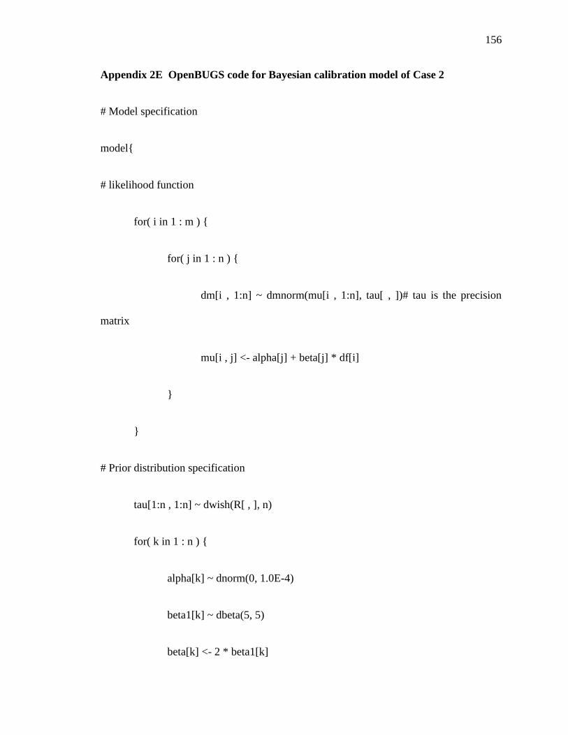
156

Appendix 2E OpenBUGS code for Bayesian calibration model of Case 2

# Model specification

model{

# likelihood function

for( i in 1 : m ) {

for( j in 1 : n ) {

dm[i , 1:n] ~ dmnorm(mu[i , 1:n], tau[ , ])# tau is the precision

matrix

mu[i , j] <- alpha[j] + beta[j] * df[i]

}

}

# Prior distribution specification

tau[1:n , 1:n] ~ dwish(R[ , ], n)

for( k in 1 : n ) {

alpha[k] ~ dnorm(0, 1.0E-4)

beta1[k] ~ dbeta(5, 5)

beta[k] <- 2 * beta1[k]

157

}

# Output analysis

Sigma.epsilon[1:n , 1:n] <- inverse(tau[ , ])

for (s in 1 : n){

for (t in 1 : n) {

rho [s, t]<-Sigma.epsilon[s, t] / sqrt(Sigma.epsilon[s, s] *

Sigma.epsilon[t, t])

}

}

}# End of the model

# Data

list(dm = structure(

.Data = c(dm[1, 1], …,dm[1, n],

dm[2, 1], …, dm[2, n],

…

…

dm[m-1, 1], …, dm[m-1, n],

dm[m, 1], …, dm[m, n],

158

.Dim = c(m, n)),

df = c(df[1], df[2], …, df[i], …, df[m]),

m =128, n = 3,

R = structure(

.Data = c(0.001, 0, 0,

0, 0.001, 0,

0, 0, 0.001),

.Dim = c(3, 3)))

# Assignment of initial values for chain1

list (tau = structure(

.Data = c(0.01, 0, 0,

0, 0.01, 0,

0, 0, 0.01),

.Dim = c(3, 3)),

alpha = c(0, 0, 0), beta1= c(0.5, 0.5, 0.5))

159

# Assignment of initial values for chain2

list(tau = structure(

.Data = c(0.05, 0, 0,

0, 0.05, 0,

0, 0, 0.05),

.Dim = c(3, 3)),

alpha = c(1, 1, 1), beta1= c(0.3, 0.3, 0.3))

160

Appendix 3A Derivation of the Conditional Posterior Distributions of

the HBM corrosion growth model

1. daij

Likelihood:

By combining Eqs. (3.7) and (3.8d), we can write the prior distribution of daij as follows:

, which is iid for i = 1, 2, …, m; and independent for j = 1,

2, …, n.

Therefore, the conditional posterior distribution of daij (i = 1, 2, …, m; j = 1, 2, …, n) can

be derived as follows:

2. ai

Likelihood:

161

Prior distribution:

Conditional posterior distribution:

Hence,

3. bi

Likelihood:

162

Prior distribution:

Conditional posterior distribution:

4. toi

Likelihood:

Prior distribution:

Conditional posterior distribution:

163

5. i2

Likelihood:

Prior distribution of 1/i2:

Therefore, the prior distribution of i2

is

, where = 1/p

Conditional posterior distribution:

Hence,

164

6. a (b)

Likelihood:

Prior distribution:

Conditional posterior distribution:

Hence,

Similarly,

165

7. a2

(b2)

Likelihood:

Prior distribution of 1/a2:

Therefore, the prior distribution of a2 is

, where = 1/f

Conditional posterior distribution:

Hence,

Similarly,

, where = 1/l

166

Appendix 3B OpenBUGS code for HBM model of Case 1

# model specification

model {

for( i in 1 : m ) {

dm[i , 1:n]~dmnorm(mu[i, 1:n] , tau1[, ]) #tau1 is the precision matrix, i.e. tau1=-1

.

for(j in 1: n) {

mu[i, j]<-alpha[j] +beta[j]*da[i, j]

da[i, j]~dnorm(dma[i, j], tau.eta[i])

dma[i, j]<-a[i] *pow((t[i, j]-to[i] ), b[i])

}

a[i]~dnorm(mu.a, tau.a)T(0, ) # “T” denotes truncation

b[i] ~dnorm(mu.b, tau.b)T(0, )

to[i]~dunif(0, t1)

tau.eta[i]~dgamma(0.001, 0.001)

sigma.eta[i]<-1/sqrt(tau.eta[i])

dp[i, 1]<-a[i] *pow((36-to[i] ), b[i]) # Prediction depth

dp[i, 2]<-a[i] *pow((37-to[i] ), b[i])

dp[i, 3]<-a[i] *pow((38-to[i] ), b[i])

dp[i, 4]<-a[i] *pow((39-to[i] ), b[i])

dp[i, 5]<-a[i] *pow((40-to[i] ), b[i])

}

mu.a~dnorm(0, 0.0001)T(0, )

167

mu.b ~dnorm(0, 0.0001)T(0, )

tau.a~dgamma(0.01, 100)

tau.b~dgamma(0.01, 100)

tau1[1:n, 1:n]<-inverse(var[1:n, 1:n])

var[1, 1]<-35.73

var[1, 2]<-29.30

var[1, 3]<-37.88

var[2, 1]<-29.30

var[2, 2]<-35.73

var[2, 3]<-38.05

var[3, 1]<-37.88

var[3, 2]<-38.05

var[3, 3]<-82.28

}

# Data

list(alpha=c(2.04, 2.04, -15.28), beta=c(0.97, 0.97, 1.40),

dm = structure(

.Data = c(dm[1, 1], dm[1, 2], dm[1, 3],

dm[2, 1], dm[2, 2], dm[2, 3],

…

…

dm[m-1, 1], dm[m-1, 2], dm[m-1, 3],

dm[m, 1], dm[m, 2], dm[m, 3],

168

.Dim = c(m, 3)),

m =62, n= 3,

t = structure(

.Data = c(28, 32, 35,

28, 32, 35,

…

…

28, 32, 35)

.Dim = c(62, 3)))

# Assignment of initial values for chain1

list(mu.a=10, mu.b=0.8, tau.a=0.05, tau.b=0.05,

tau.eta=c(0.01, 0.01, 0.01, 0.01, 0.01, 0.01, 0.01, 0.01, 0.01, 0.01, 0.01, 0.01, 0.01, 0.01,

0.01, 0.01, 0.01, 0.01, 0.01, 0.01, 0.01, 0.01, 0.01, 0.01, 0.01, 0.01, 0.01, 0.01, 0.01, 0.01,

0.01, 0.01, 0.01, 0.01, 0.01, 0.01, 0.01, 0.01, 0.01, 0.01, 0.01, 0.01, 0.01, 0.01, 0.01, 0.01,

0.01, 0.01, 0.01, 0.01, 0.01, 0.01, 0.01, 0.01, 0.01, 0.01, 0.01, 0.01, 0.01, 0.01, 0.01,

0.01),

a=c(10, 10, 10, 10, 10, 10, 10, 10, 10, 10, 10, 10, 10, 10, 10, 10, 10, 10, 10, 10, 10, 10,

10, 10, 10, 10, 10, 10, 10, 10, 10, 10, 10, 10, 10, 10, 10, 10, 10, 10, 10, 10, 10, 10, 10, 10,

10, 10, 10, 10, 10, 10, 10, 10, 10, 10, 10, 10, 10, 10, 10, 10),

b=c(0.3, 0.3, 0.3, 0.3, 0.3, 0.3, 0.3, 0.3, 0.3, 0.3, 0.3, 0.3, 0.3, 0.3, 0.3, 0.3, 0.3, 0.3, 0.3,

0.3, 0.3, 0.3, 0.3, 0.3, 0.3, 0.3, 0.3, 0.3, 0.3, 0.3, 0.3, 0.3, 0.3, 0.3, 0.3, 0.3, 0.3, 0.3, 0.3,

0.3, 0.3, 0.3, 0.3, 0.3, 0.3, 0.3, 0.3, 0.3, 0.3, 0.3, 0.3, 0.3, 0.3, 0.3, 0.3, 0.3, 0.3, 0.3, 0.3,

0.3, 0.3, 0.3),

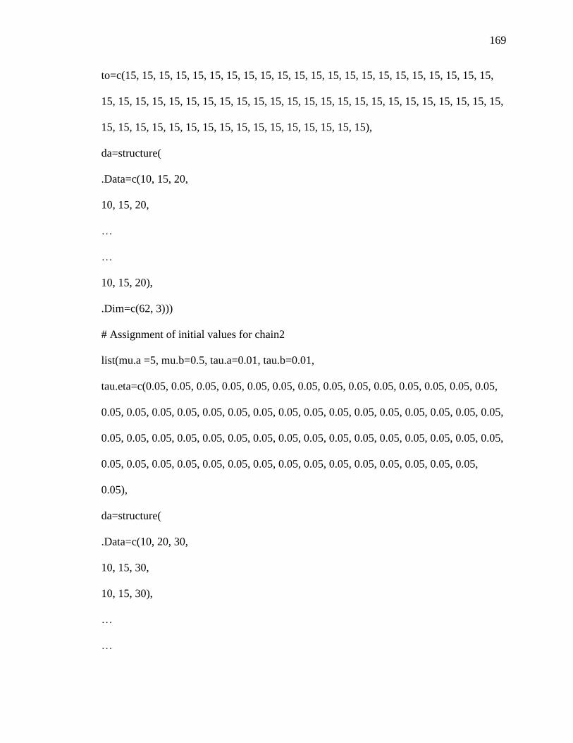
169

to=c(15, 15, 15, 15, 15, 15, 15, 15, 15, 15, 15, 15, 15, 15, 15, 15, 15, 15, 15, 15, 15, 15,

15, 15, 15, 15, 15, 15, 15, 15, 15, 15, 15, 15, 15, 15, 15, 15, 15, 15, 15, 15, 15, 15, 15, 15,

15, 15, 15, 15, 15, 15, 15, 15, 15, 15, 15, 15, 15, 15, 15, 15),

da=structure(

.Data=c(10, 15, 20,

10, 15, 20,

…

…

10, 15, 20),

.Dim=c(62, 3)))

# Assignment of initial values for chain2

list(mu.a =5, mu.b=0.5, tau.a=0.01, tau.b=0.01,

tau.eta=c(0.05, 0.05, 0.05, 0.05, 0.05, 0.05, 0.05, 0.05, 0.05, 0.05, 0.05, 0.05, 0.05, 0.05,

0.05, 0.05, 0.05, 0.05, 0.05, 0.05, 0.05, 0.05, 0.05, 0.05, 0.05, 0.05, 0.05, 0.05, 0.05, 0.05,

0.05, 0.05, 0.05, 0.05, 0.05, 0.05, 0.05, 0.05, 0.05, 0.05, 0.05, 0.05, 0.05, 0.05, 0.05, 0.05,

0.05, 0.05, 0.05, 0.05, 0.05, 0.05, 0.05, 0.05, 0.05, 0.05, 0.05, 0.05, 0.05, 0.05, 0.05,

0.05),

da=structure(

.Data=c(10, 20, 30,

10, 15, 30,

10, 15, 30),

…

…

170

.Dim=c(62, 3)),

a=c(15, 15, 15, 15, 15, 15, 15, 15, 15, 15, 15, 15, 15, 15, 15, 15, 15, 15, 15, 15, 15, 15,

15, 15, 15, 15, 15, 15, 15, 15, 15, 15, 15, 15, 15, 15, 15, 15, 15, 15, 15, 15, 15, 15, 15, 15,

15, 15, 15, 15, 15, 15, 15, 15, 15, 15, 15, 15, 15, 15, 15, 15),

b=c(0.6, 0.6, 0.6, 0.6, 0.6, 0.6, 0.6, 0.6, 0.6, 0.6, 0.6, 0.6, 0.6, 0.6, 0.6, 0.6, 0.6, 0.6, 0.6,

0.6, 0.6, 0.6, 0.6, 0.6, 0.6, 0.6, 0.6, 0.6, 0.6, 0.6, 0.6, 0.6, 0.6, 0.6, 0.6, 0.6, 0.6, 0.6, 0.6,

0.6, 0.6, 0.6, 0.6, 0.6, 0.6, 0.6, 0.6, 0.6, 0.6, 0.6, 0.6, 0.6, 0.6, 0.6, 0.6, 0.6, 0.6, 0.6, 0.6,

0.6, 0.6, 0.6),

to=c(10, 10, 10, 10, 10, 10, 10, 10, 10, 10, 10, 10, 10, 10, 10, 10, 10, 10, 10, 10, 10, 10,

10, 10, 10, 10, 10, 10, 10, 10, 10, 10, 10, 10, 10, 10, 10, 10, 10, 10, 10, 10, 10, 10, 10, 10,

10, 10, 10, 10, 10, 10, 10, 10, 10, 10, 10, 10, 10, 10, 10, 10))

171

Appendix 3C OpenBUGS code for HBM model of Case 2

# model specification

model {

for( i in 1 : m ) {

dm[i , 1:n]~dmnorm(mu[i, 1:n] , tau1[, ])

for(j in 1: n) {

mu[i, j]<-alpha[j] +beta[j]*da[i, j]

da[i, j]~dnorm(dma[i, j], tau.eta[i])

dma[i, j]<-a[i] *pow((t[i, j]-to[i] ), b[i])

}

a[i]~dnorm(mu.a, tau.a)T(0, )

b[i] ~dnorm(mu.b, tau.b)T(0, )

to[i]~dunif(0, 28)

dp[i, 1]<-a[i] *pow((38-to[i] ), b[i]) # Prediction depth

dp[i, 2]<-a[i] *pow((39-to[i] ), b[i])

dp[i, 3]<-a[i] *pow((40-to[i] ), b[i])

tau.eta[i]~dgamma(0.001, 0.001)

sigma.eta[i]<-1/sqrt(tau.eta[i])

}

mu.a~dnorm(0, 0.0001)T(0, )

mu.b~dnorm(0, 0.0001)T(0, )

tau.a~dgamma(0.01, 100)

172

tau.b~dgamma(0.01, 100)

tau1[1:n, 1:n]<-inverse(var[1:n, 1:n])

var[1, 1]<-28.35

var[1, 2]<-28.87

var[1, 3]<-31.44

var[2, 1]<-28.87

var[2, 2]<-50.75

var[2, 3]<-38.75

var[3, 1]<-31.44

var[3, 2]<-38.75

var[3, 3]<-58.71

}

# Data

list(alpha=c(-4.23, -9.50, -3.54), beta=c(0.89, 0.91, 1.00),

t = structure(

.Data=c(32, 35, 37,

32, 35, 37,

…

…

32, 35, 37),

.Dim = c(60, 3)),

m = 60, n = 3,

dm = structure(

173

.Data = c(dm[1, 1], dm[1, 2], dm[1, 3],

dm[2, 1], dm[2, 2], dm[2, 3],

…

…

dm[m-1, 1], dm[m-1, 2], dm[m-1, 3],

dm[m, 1], dm[m, 2], dm[m, 3],

.Dim = c(m, 3)))

# Assignment of initial values for chain1

list(mu.a=5, mu.b=0.5, tau.a=0.01, tau.b=0.01,

tau.eta=c(0.01, 0.01, 0.01, 0.01, 0.01, 0.01, 0.01, 0.01, 0.01, 0.01, 0.01, 0.01, 0.01, 0.01,

0.01, 0.01, 0.01, 0.01, 0.01, 0.01, 0.01, 0.01, 0.01, 0.01, 0.01, 0.01, 0.01, 0.01, 0.01, 0.01,

0.01, 0.01, 0.01, 0.01, 0.01, 0.01, 0.01, 0.01, 0.01, 0.01, 0.01, 0.01, 0.01, 0.01, 0.01, 0.01,

0.01, 0.01, 0.01, 0.01, 0.01, 0.01, 0.01, 0.01, 0.01, 0.01, 0.01, 0.01, 0.01, 0.01),

a=c(10, 10, 10, 10, 10, 10, 10, 10, 10, 10, 10, 10, 10, 10, 10, 10, 10, 10, 10, 10, 10, 10,

10, 10, 10, 10, 10, 10, 10, 10, 10, 10, 10, 10, 10, 10, 10, 10, 10, 10, 10, 10, 10, 10, 10, 10,

10, 10, 10, 10, 10, 10, 10, 10, 10, 10, 10, 10, 10, 10),

b=c(0.5, 0.5, 0.5, 0.5, 0.5, 0.5, 0.5, 0.5, 0.5, 0.5, 0.5, 0.5, 0.5, 0.5, 0.5, 0.5, 0.5, 0.5, 0.5,

0.5, 0.5, 0.5, 0.5, 0.5, 0.5, 0.5, 0.5, 0.5, 0.5, 0.5, 0.5, 0.5, 0.5, 0.5, 0.5, 0.5, 0.5, 0.5, 0.5,

0.5, 0.5, 0.5, 0.5, 0.5, 0.5, 0.5, 0.5, 0.5, 0.5, 0.5, 0.5, 0.5, 0.5, 0.5, 0.5, 0.5, 0.5, 0.5, 0.5,

0.5),

to=c(10, 10, 10, 10, 10, 10, 10, 10, 10, 10, 10, 10, 10, 10, 10, 10, 10, 10, 10, 10, 10, 10,

10, 10, 10, 10, 10, 10, 10, 10, 10, 10, 10, 10, 10, 10, 10, 10, 10, 10, 10, 10, 10, 10, 10, 10,

10, 10, 10, 10, 10, 10, 10, 10, 10, 10, 10, 10, 10, 10),

174

da=structure(

.Data=c(10, 20, 30,

10, 20, 30,

…

…

10, 20, 30),

.Dim=c(60, 3)))

# Assignment of initial values for chain1

list(mu.a=10, b.m=0.8, mu.b=0.05, tau.b=0.05,

tau.eta=c(0.05, 0.05, 0.05, 0.05, 0.05, 0.05, 0.05, 0.05, 0.05, 0.05, 0.05, 0.05, 0.05, 0.05,

0.05, 0.05, 0.05, 0.05, 0.05, 0.05, 0.05, 0.05, 0.05, 0.05, 0.05, 0.05, 0.05, 0.05, 0.05, 0.05,

0.05, 0.05, 0.05, 0.05, 0.05, 0.05, 0.05, 0.05, 0.05, 0.05, 0.05, 0.05, 0.05, 0.05, 0.05, 0.05,

0.05, 0.05, 0.05, 0.05, 0.05, 0.05, 0.05, 0.05, 0.05, 0.05, 0.05, 0.05, 0.05, 0.05),

a=c(5, 5, 5, 5, 5, 5, 5, 5, 5, 5, 5, 5, 5, 5, 5, 5, 5, 5, 5, 5, 5, 5, 5, 5, 5, 5, 5, 5, 5, 5, 5, 5, 5, 5,

5, 5, 5, 5, 5, 5, 5, 5, 5, 5, 5, 5, 5, 5, 5, 5, 5, 5, 5, 5, 5, 5, 5, 5, 5, 5),

b=c(0.3, 0.3, 0.3, 0.3, 0.3, 0.3, 0.3, 0.3, 0.3, 0.3, 0.3, 0.3, 0.3, 0.3, 0.3, 0.3, 0.3, 0.3, 0.3,

0.3, 0.3, 0.3, 0.3, 0.3, 0.3, 0.3, 0.3, 0.3, 0.3, 0.3, 0.3, 0.3, 0.3, 0.3, 0.3, 0.3, 0.3, 0.3, 0.3,

0.3, 0.3, 0.3, 0.3, 0.3, 0.3, 0.3, 0.3, 0.3, 0.3, 0.3, 0.3, 0.3, 0.3, 0.3, 0.3, 0.3, 0.3, 0.3, 0.3,

0.3),

to=c(20, 20, 20, 20, 20, 20, 20, 20, 20, 20, 20, 20, 20, 20, 20, 20, 20, 20, 20, 20, 20, 20,

20, 20, 20, 20, 20, 20, 20, 20, 20, 20, 20, 20, 20, 20, 20, 20, 20, 20, 20, 20, 20, 20, 20, 20,

20, 20, 20, 20, 20, 20, 20, 20, 20, 20, 20, 20, 20, 20),

da=structure(

175

.Data=c(10, 15, 25,

10, 15, 25,

…

…

10, 15, 25),

.Dim=c(60, 3)))

176

Curriculum Vitae

Name: Mohammad Al-Amin

Birth Place Brahmanbaria, Bangladesh

Date of Birth 06 June, 1986

Post-secondary Bangladesh University of Engineering and Technology

Education: Dhaka, Bangladesh

2004-2009, B.Sc. (Civil Engineering)

The University of Western Ontario

London, Ontario, Canada

2010-2012, M.E.Sc. (Structural Engineering)

Honours and Dutch-Bangla Bank Foundation Scholarship

Awards: 2004-2009

Graduate Thesis Research Award

The University of Western Ontario

2011-2012

Related Work Junior Engineer

Experience PNJ Associates

Dhaka, Bangladesh

01/11/2009-15/08/2010

Research and Teaching Assistant

The University of Western Ontario

2010-2012