,.

"BAYES' THEOREM" FOR UTILITY

by

Leigh Tesfatsion

Discussion Paper No. 76-65, April 1976

Center for Economic Research

Department 0 f Economics

University of Minnesota

Minneapolis, Minnesota 55455

ABSTRACT

An algorithm is proposed for updating an initial

period objective (risk) function by means of transitional

utility (loss) assessments, in a manner analogous to Bayes'

theorem for probability. Specification of updated probability

assessments is not required. The algorithm is shown to be

robust wi°th respect to a fully updated procedure, given certain

empirically meaningful restrictions. Existence of the initial

period objective function is axiomatized in the context of a

model which adopts a symmetrical approach to utility and

probability.

"BAYES' THEOREM" FOR UTILITY*

by

Leigh Tesfatsion

1. INTRODUCTION

The principal purpose of this paper is to propose a simple

"utility algorithm" for updating an initial period objective (risk)

function by means of transitional utility (loss) assessments, in a

manner analogous to Bayes' theorem for probabi1ity.1 Specification

of updated probability assessments is not required. The algorithm is

shown to be robust with respect to a fully updated procedure, given

certain empirically meaningful restrictions.

The computation and information required for the numerical solu-

tion of Bayesian sequential decision procedures is often prohibitive

(see DeGroot [2, Part Four]). Consequently, for sequential decision

problems in which utility assessments are relatively straightforward

and probability assessments are vague or of intractable form, a

utility algorithm may be a desirable alternative to a Bayesian pro-

2 cedure. Numerous interesting economic decision problems fit this

description; for many important economic time series appear to be

realizations for nonstationary stochastic processes, difficult to

express analytically in any convincing manner, and intractable to

work with even if so expressed. In contrast, utility assessments

over outcomes can often be based on relatively noncontroversial

revenue and cost considerations. 3

*Research for this paper was supported by National Science Foundation Grant GS-31276X, University of Minnesota.

,I

,I

2

A seemingly essential prerequisite for devising general utility

algorithms is that utility be interpreted as the proper twin of prob­

ability. Statistical studies have generally emphasized probability

distributions, with utility (loss, cost .•• ) assessments specified in

abstract or routine (e.g. quadratic) form when they appear. Never­

theless, like probability, utility can be interpreted as a possibly

conditioned distribution of "mass" over a collection of relevant

events, however these are represented (e.g.~ sets, points, proposi­

tions .•. ). Indeed, it has been cogently argued by de Finetti [1, 2.4]

that in practice any distinction drawn between events to be represented

as sets and events to be represented as points is purely a matter of

convenience. Events, as distinct from sets, can always be subdivided

by setting out their description in finer detai1. 4

The following concepts indicate the extent to which a meaningful

analogy between utility and probability can be made.

utility density

u: &1 + R

where R = the real line and u(w) - the utility (loss, cost •.• ) the

decision maker associates with the realization of the event w € &1.

conditioned utiZity densities

u (-Ie): &1+R, e €@,

where u(wle) = the utility (loss, cost ••. ) the decision maker associ­

ates with the realization of event w € &1, conditioned on the reali­

zation (choice, hypothesis, truth ••• ) of e.

,I

nth period transitionaZ utiZity density

u (0 Iw1 , ••. ,wn_1): nn + R,

where the event space n relevant for period n is a function n

3

n(w1

, .•• ,wn_1) of the realized event stream (w1 ' ..• ,wn

_1) E n1

x ••• xnn_1'

and u(w Iw1 , ..• ,w 1) = the utility (loss, cost ••• ) the decision maker n n-

associates with the realization of event WEn , conditioned on the n n

Markov utiZity density of order 1

u(w Iw1 ,.··,w 1) = u(w lw 1): n + R; n n- n n- n

i.e., the utility (loss, cost ••. ) the decision maker associates with

the realization of event w in period n is independent of the events n

(w1

' .•. ,wn

_2

) which he observed previous to period n-1. (One inter-

pretation might be that habit formation is insignificant for the

decision maker.) Generalization to other orders is obvious. In

particular, a Markov utility density of order 0 might be termed a

stationary utiZity density.

The utility algorithm proposed in this paper will require a

period by period specification of conditioned transitional utility

densities.

The paper is organized as follows. The algorithm is presented

in section 4 and its properties are investigated in section 5. The

definition of the algorithm and many of the properties established

for the algorithm are independent of the exact form of the initial

period objective function U. However, as shown in section 5, it is

,t

4

useful to assume that U has a general expected utility representation

u(a) =1 rl(a)u(wla)p(dwla),aEtEl, (1.1)

where tEl = {a, •.• } is a choice set consisting of "policies," and for

each policy e £ tEl, u(·1 a) is a a-conditioned utility density, p (·1 a)

is a a-conditioned probability measure, and rl(8) is a set of atomic

events relevant for the initial period choice of a. As shown in the

preliminary sections 2 and 3, the representation (1.1) for U can be

axiomatized in terms of primitive sets and relations.

The algorithm is derived recursively from a "Bayes' theorem

for utility" of the form

u(alwl ) oc u(wlla) + u(a). (1.2)

Intuitively, (1. 2) asserts that the "posterior" utility U( 81 wI) which

the decision maker associates with the choice of policy a for period

2 after having observed event wI in period 1 is proportional to the

preobservation utility u(wlla) he associated with the realization of

event wI in period 1, conditioned on the choice of policy a for period

1, weighted by the "prior" (preobservation) utility U(a) he associated

with the choice of policy 8 for period 1. For uniform (constant)

priors U, (1.2) asserts that in period 2 the decision maker ought to

choose the policy that would have given him maximum utility in period

1 for the realized wI (a "maximum likelihood method" for utility - see

section 5). As will be clarified in sections 4 and 5, for certain

repetitive decision problems u(·lwl

) represents a reasonable choice

of objective function for period 2.

For example, consider the following situation. A decision maker

is about to introduce a perishable good into a market in the face of

uncertain demand. Periodically he Will have to order new stock a

"

,1

S

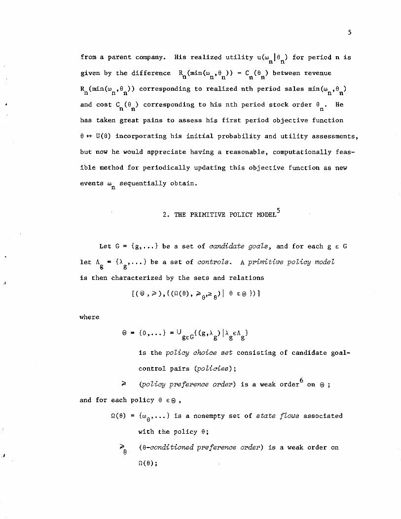
from a parent company. His realized utility u(w Ie ) for period n is n n

given by the difference R (min(w ,e » - c (e ) between revenue n n n n n

R (min(w ,e » corresponding to realized nth period sales min(w ,e ) n n n n n

and cost C (e ) corresponding to his nth period stock order e. He n n n

has taken great pains to assess his first period objective function

e ~ U(e) incorporating his initial probability and utility assessments,

but now he would appreciate having a reasonable, computationally feas-

ible method for periodically updating this objective function as new

events w sequentially obtain. n

2. THE PRIMITIVE POLICY MODELS

Let G = {g, ... } be a set of candidate goals~ and for each g E G

let A = {A , ••• } be a set of controls. A primitive policy model g g

is then characterized by the sets and relations

where

[(®,p),{(Q(e), Pe'~e)1 e E@})]

@ = {e, .•• } = U G{(g,A )IA EA } gE g g g

is the policy choice set consisting of candidate goal-

control pairs (policies);

6 (policy preference order) is a weak order on @

and for each policy e E @ ,

Q(e) {we' ..• } is a nonempty set of state flows associated

with the policy e;

(e-conditioned preference order) is a weak order on

Q(e);

. '

~e (a-conditioned ppobabiZity opdep)is a weak order on the

algebra7 2

Q(a) comprising all subsets (event ftows)

RemQPk: Axiomatic theories for the state-consequence-act models

6

prevalent in economic and statistical decision theory generally assume

the existence of only one primitive order, a preference order over acts,

and hence obtain a simpler statement for their primitives. Nevertheless,

the axioms used to justify an expected utility representation for the

preference order then invariably impose strong nonnecessary restrictions

on the primitives (e.g., L.J. Savage's reliance on constant acts in

[5]). In contrast, assuming each state flow set Q(a) is finite, neces-

sary and sufficient conditions can be given which justify an expected

utility representation for the policy preference order ~ (see section

3 below) .•.

The controls may be interpreted as possibly conditioned sequences

of actions (i.e., partial contingency plans) entirely under the deci-

sion maker's control at the time of his choice. The candidate goals

g e: G may be interpreted as potential objectives (e. g., production

targets, intervals for quality control, ••. ) whose realization the

decision maker can attempt to achieve through appropriate choice of a

control. The grouping of the controls into sets {A Ige:G} reflects g

the possibility that different sets of controls may be relevant for

different goals. A control A e:A mayor may not provide for the com­g g

munication of the goal g to other persons in the decision maker's

problem environment.

The weak order~ on @ can be interpreted as a preference order

"

7

as follows. For all 8,8'£ @,

8 ~8' <=> the choice of policy 8 is at least

as desirable to the decision maker

at the choice of policy 8'.

It is assumed that the decision maker will choose a policy (candidate

* goal-control pair) 8* £@ which is optimal in the sense that 8 '" a for all

a £ @.

control

Throughout this paper "choose policy a = (g,A )" and "implement g

A with g as the objective" are used interchangeably. g

For each a £8, the set n(a) of state flows wa can be interpreted

as the decision maker's answer to the following question: "If I choose

policy a, what distinct situations (Le., state flows wa) might obtain?"

The state flows may include references to past, present, and future

happenings. In particular, they can subsume both the "states" and the

"consequences" of traditional state-consequence-act models.

The a-conditioned preference orders "'a can be interpreted as fol­

lows. For all w, w' £ n(a),a £@,

w ~a w' <=> the realization of w is at least

as desirable to the decision maker as

the realization of w', given that he

chooses a.

Similarly, the a-conditioned probability orders> can be interpreted --e as follows. For all E, E' £ 2n (a), a £@ ,

E > E' <=> in the decision maker's judgment the -a

realization of E is at least as likely

as the realization of E', given that he

chooses a.

As usual, all preference and probability orders depend (here implicitly)

on the decision maker's current information state.

"

8

A state flow w may be relevant for the decision maker's problem

under distinct potential policy choices; e.g., w £ n(e)nn(e') for some

e,e' £9. Given state flows w,w' £ n(e)nn(a') for some e,e' £@, it

may hold that w ~e w'whereas w' ~e'w. Verbally, the relative desir­

ability of the state flows wand w' may depend on which conditioning

event the decision maker is considering, "I choose e" or "I choose e'."

Similarly for the relative likelihood of event flows.

Examples illustrating these interpretations are given in Tesfat-

sion [6] and [8].

3. OBJECTIVE FUNCTION REPRESENTATION

In Tesfatsion [7] necessary and sufficient conditions are given

which ensure that a primitive policy model with finite state flow sets

n(e) has an expected utility (objective function) representation in

the following sense. To each policy e £@ there corresponds a finitely

additive probability measure p(ole):2n(e)+ [0,1] satisfying

p(EI e) ~ p(E' I e) <=> E > E'· -e ' (3.1)

for all E, E' £ 2n (e), and a utility function u(ole):n(e)+R satisfying

. u(wle) ~ u(w'le) <=> w ~e

for all w,w' £ n(e), such that

for all e, e' £ @.

w' , (3.2)

(3.3)

The representation (3.1)-(3.3) for the preference order ~ can

be interpreted as follows. To each state flow w £ n(e),e £@ , the

decision maker assigns a number u(wle) representing the desirability

of w, given he chooses e, and a number p(wle) representing the

likelihood of w, given he chooses e. He then calculates the expected

utility

corresponding to each choice of policy e € @, and chooses a policy

which yields maximum expected utility.

Definition: A primitive policy model with representation as in

(3.1)-(3.3) will be referred to as a policy model characterized by a

vector

with objective function u:@ ~ R given by

The principal distinctive feature of the policy model is the

9

symmetrical treatment of utility and probability assessments. Both are

conditioned on policy choices, and both are defined over "state flows"

rather than having utility defined over a set of "consequences" and

probability defined over a set of "states."

The conditioning of the utility functions {u(·le):Q(e)~Rle€@} and

the probability measures {p(·le):2Q(e)~ [o,l]le€@} on the policies e

is often essential; for, as illustrated by examples in Tesfatsion [6]

and [8], a state flow may have a different utility and probability de-

pending on which policy is chosen. By subsuming states and consequences

into state flows and defining utility over state flows rather than con­

sequences alone, the practical difficulty of specifying utility-free

states can be avoided. More important, when probability is defined

over state flows subsuming both states and consequences, it is no longer

10

necessary for the decision maker to specify his available actions in

the form of complete contingency plans (e.g., Savage acts, von Neumann

strategies, Wald decision functions •.. ) mapping states into conse-

quences. For this reason the policy model appears to be more suitable

than traditional state-consequence-act models for modeling certain

limited information decision problems.

As will be discussed in sections 4 and 5, an additional benefit

to be gained from the symmetrical treatment of utility and probability

is the possibility of updating the initial objective function through

transitional utility assessments in a manner analogous to Bayes'

theorem for probability.

4. THE ALGORITHM

Let sl represent the initial information state of a decision maker

facing a policy selection problem at some time tl

. Suppose his prob­

lem has the following policy model form (cf. section 3):

I Ql(ro I r 1 :: ( ® l' {ul (0 Ie) : Ql (e )-+R e £ @ 1 } ,{ PI (0 Ie) : 2 -+ [0,1] e£ @ I})

with objective function

where the policy choice set @l and state flow sets Ql(e) are functions

of his information state sl' and ul

(ole), Pl(o Ie), and ul(e) are abbre­

viations for u(olsl,e), p(o ISl,e), and u(elsl ) respectively.8

Presumably, if rl

is well-defined, the decision maker at some

future time t2 (uncertain as of time t l ) will have implemented the

* policy 81 chosen at time tl and verified the realization of one (and

* * only one) state flow WI £ nl (8l ). His new information state at time

t2 will then be s2 A subsequent policy selection

problem might then have the policy model form

r 2 :: (82,{u2(o'8):n2(8)+RI8£82},{P2(o,8):2n2(8)+[O,1]18£82})

with updated objective function I

U2(8) :: J n (8)u2 (wI8) P2(dwI8), 8 £ 8 2, 2

(4.1)

11

where the policy choice set 8 2 and state flow sets n2 (8) are functions

of his new information state s2' and u2(ols), P2(oI8), and U2 (8) are

abbreviations for u(ols2,8), P(ols2,8), and U(8Is2) respectively.

If the policy choice set 8 2 or the state flow sets n2

(8) contain

numerous alternatives, it may not be feasible or desirable for the

decision maker to carry out all the updating required by r 2• If

8 1 = 8 2 :: 8 and one state flow set n is relevant for all policies in

both periods, the decision maker could replace (4.1) by the updated

objective function

* * Ul(8Iwl)a:ul(wlI8) +Ul (8), 8 £8. (4.2)

* Intuitively, (4.2) asserts that the posterior utility Ul(8Iwl)

which the decision maker associates with the choice of policy 8 for

* period 2 following the realization of WI in period 1 is proportional

* to the preobservation utility ul(wlI8) he associated with the reali-

* zation of WI in period 1, conditioned on the choice of policy 8 for

period 1, weighted by the prior (preobservation) utility Ul (8) he

associated with the choice of policy 8 for period 1. Policies 8

* which score better with respect to the realized state flow WI than

their anticipated "average" Ul

(8) have their relative utility value

12

raised for period 2; conversely for those policies which score lower

than anticipated. For repetitive decision problems in which the state

flows are judged by the decision maker to be approximately stochasti-

cally independent of his policy choices, i.e., for all W € Q and

e € e,

and the costs incurred by switching policies from period to period are

* negligible, ul(·lwl ) may represent a reasonable choice of objective

function for period 2. 9

By taking exponents in (4.2), an exact analogy with Bayes' theorem

for probability is obtained; namely,

* * vl(elwl ) ~ vl(wlle) Vl(e), (4.3)

* where Vl(e) = exp(ul(e», vl(wlle) * * = exp(ul(wlle», and VI (elwl ) -

* * exp (ul(elwl ». Since vl(wlle) Vl(e) * and log(vl(wlle) VI (e» = * ul(wlle) + Ul (e) achieve their maxima (if any) over the same set of

policies, (4.2) and (4.3) yield the same set of policy recommendations.

The algorithm will be derived by recursion from the multiplicative re-

lation (4.3) in preference to (4.2) in order to take direct advantage

of results previously obtained by researchers investigating Bayes'

theorem for probability.

The algorithm will now be formally presented.

4.1 Assumptions and Notation

At some time tl a decision maker in a certain information state

* * sl faces a decision problem requiring periodic policy choices el ,e 2,···.

A single policy choice set @=e (sl) is relevant for each period

[tn,tn+l ], n ~ 1, and a single state flow set Q=Q(sl) is relevant for

13

all policies in all periods. In addition, the cost of switching poli­

* cies from period to period is negligible; i.e., letting w. denote J

the state flow which obtains in period j, the decision maker's

policy-conditioned transitional utility densities {u (·1 S) :Q+RI SEe} n

for period n satisfy

li (wIS) n

* * = u(wlsl,wl,···,wn_l,S),

for all w E Q and S E 8. Finally, the decision maker is able to give

initial period policy-conditioned probability assessments {Pl(-IS):

2Q+[O,1]ls Ee} for the likelihood of the event flows EC 2Q.

For normalization purposes it will be assumed that for some posi-

tive measure mover e all integrals

J@f(S)m(dS)

appearing in the algorithm are well-defined and satisfy

J If(S)lm(dS) < 00. e For example, if e is finite, m could denote counting measure.

4.2 The Algorithm

Step 0: Calculate the initial period objective function Ul : 8+R,

given by

and select a policy S~E® for period 1 which satisfies

v Vl(8J)~ Vl(S),

for all S E 8, where

* Step n (n ~ 1): Verify a state flow wn E Q in period n; calculate

the updated objective function Vn+l :8+R for period n+l, given by

14

Vn+l(e) - (4.4)

where

* * v (w Ie) = exp (u (w Ie », n n n n

* v (w ) -n n

* r(.";\v (w (e») v (e)m(de); Jrt; n n n

v and select a policy en+l E @ for period n+l which satisfies

v Vn+l (en+l ) ~ Vn+l (e), for all e E @ •

Remark: All factors in (4.4) are strictly positive. The normal­

* izing factors v (w ) guarantee that n n

JV (e)m(de) = 1, n > 2. @n

Since Ul

is only unique up to positive linear transformation under

the axiomatization discussed in section 3, VI = exp(Ul ) can be

similarly normalized.

5. ROBUSTNESS AND SMALL SAMPLE PROPERTIES

Certain "small sample" properties of the algorithm will first be

established, followed by a number of robustness results. Although

many of the properties are formally analogous to properties previous-

ly established for probability densities, their interpretation in

terms of utility densities is equally natural and meaningful. The

robustness results have no direct analogy in probability theory.

The assumptions, notation, and definitions of 4.1 and 4.2 will

be maintained throughout this section, except where otherwise indi­

* * cated. The existence of a particular sequence wl ,w2 ••• of state

flows "realized" over periods 1, 2, •.• will be implicitly assumed

15

in the statement and proof of all theorems. The symbol K will denote n

a general nth period constant, i.e., a term independent of policy

choices and state flows to be realized in periods m>n. The exact form

of K may vary during a proof. n

5.1 Small Sample Properties

The first theorem below guarantees that the algorithm is essen-

tially invariant under similar positive linear transformation of the

utility densities.

Theorem 5.1: For each n~l, the set of maximizing policies for

the objective function V is invariant under similar positive linear n

transformation of the utility densities {U, (. 18) :S1+Rll<j<n,8e: e}. J --

Remark: The sets of maximizing policies for the V are not n

necessarily invariant under dissimilar positive linear transforma-

tions of the utility densities. The practical implication is that the

utility densities u for each period n should be scored in relation to n

a fixed origin and unit determined in the initial period.

* Proof: Let n>l be given. For each j,l~j~n, let u, = au, + b J J

* for some a, b e: R, a>O, and let V denote the nth period algorithm n

* objective function calculated in terms of the densities u,' l~j~n. J

By assumption,

Ul (8) = fnu1 (wIS)Pl (dwIS), S e: e.

Hence

and

* logVl * - log(exp(U1» = alogV1 + b. (5.1)

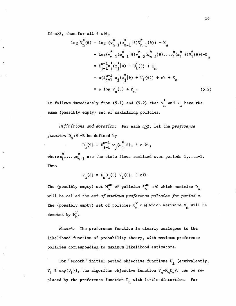
If n~2, then for all a e: El ,

* log V (a) n

16

* * * * * * * = log (vn_l (wn_l ' a)vn_2 (wn_2 ' a) ••• VI (wI' a)Vl (a»+Kn

n-l * *, * = Lj=luj(wj a) + ul(a) + Kn

n-l *, = a(Lj=l uj(wj a) + ul(a» + nb + Kn

= a log V (a) +K. (5.2) n n

* It follows immediately from (5.1) and (5.2) that V and V have the n n

same (possibly empty) set of maximizing policies.

Definitions and Notation: For each n>2, let the preference

function D :El +R be defined n

* *

n-l Dn(a) :: IIj=l

by

* v.(w.'a), J J

ae:El,

where~, ••. ,wn_l are the state flows realized over periods l, ••. n-l.

Thus

V (a) = K D (a) vl(a), a e: El • n n n

The (possibly empty) set ~p of policies amp e: El which maximize D n n n

will be called the set of maximum preference policies for period n.

The (possibly empty) set of policies aV e: El which maximize V will be

n n v denoted by M . n

Remark: The preference function is clearly analogous to the

likelihood function of probability theory, with maximum preference

policies corresponding to maximum likelihood estimators.

For "smooth" initial period objective functions Ul

(equivalently,

VI :: exp(Ul », the algorithm objective function Vn=KnDnVl can be re­

placed by the preference function D with little distortion. For n

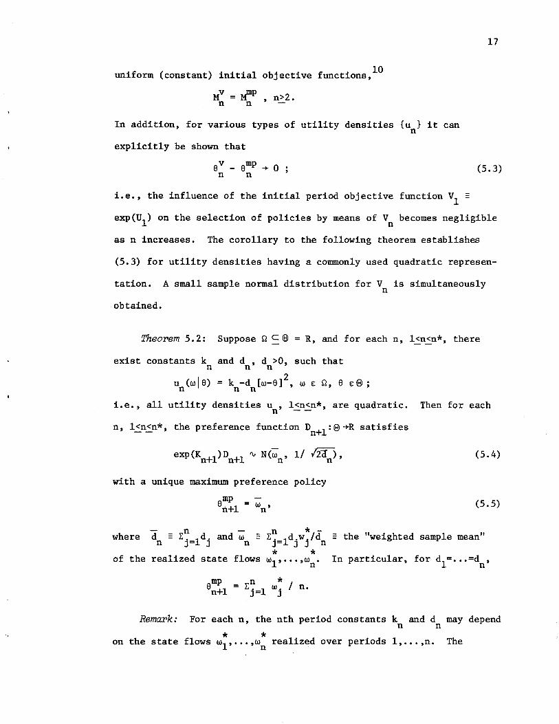
10 uniform (constant) initial objective functions,

Mv = . .mp 2 M. , n~ • n n

In addition, for various types of utility densities {u } it can n

explicitly be shown that

17

aV _ amp -+ 0 ; n n

(5.3)

i.e., the influence of the initial period objective function VI =

exp(Ul ) on the selection of policies by means of Vn becomes negligible

as n increases. The corollary to the following theorem establishes

(5.3) for utility densities having a commonly used quadratic represen-

tation. A small sample normal distribution for V is simultaneously n

obtained.

~eorem 5.2: Suppose n c@ = R, and for each n, l~n~n*, there

exist constants k and d , d >0, such that n n n

u (wla) = k -d [w_a]2, WEn, a E@; n n n

i. e. , all utility densities u , l<n<n*, are quadratic. n -- Then for each

n, l<n<n*, the preference function Dn+l:@-+R satisfies

with a unique maximum preference policy

amp n+l = wn '

(5.4)

(5.5)

where n * -- k. ld.wj/d = the "weighted sample mean" J= J n

* * of the realized state flows wl' ••• ,wn • In particular, for dl= ••• =dn ,

amp n * I n+l = kj=l Wj n.

Remark: For each n, the nth period constants k and d may depend n n

* * on the state flows wl, .•• ,wn realized over periods l, ••• ,n. The

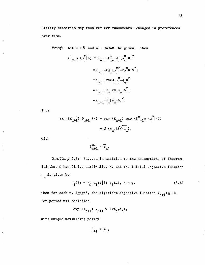
18

utility densities may thus reflect fundamental changes in preferences

over time.

Pr>oof: Let 6 E (8) and n, l<n<n*, be given. Then

Thus

with

*2 * 2 =Kn+1-~dj [wj -2wj 6+6 ]

* - 2 = Kn+1+26~djwj-dn 6

- - 2 =K +l+d [26 W -6 ] n n n

- - 2 = K -d [w -6] • n+1 n n

n *1 = exp (Kn+1) exp (~. 1u.(w .• » J= ] ]

'V N (w ,1/1id), n n

W • n

CoroZZary 5.3: Suppose in addition to the assumptions of Theorem

5.2 that Q has finite cardinality N, and the initial objective function

U1

is given by

(5.6)

Then for each n, l<n~n*, the algorithm objective function Vn+1 :(8)+R

for period n+1 satisfies

with unique maximizing policy

v 6n+1 = m ,

n

"

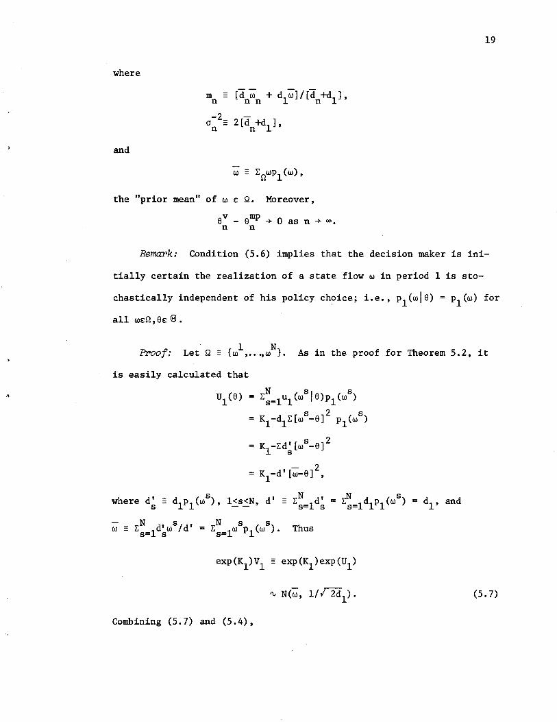
19

where

m - (d" w + dlw] /[(1 +dll, n n n n

and

w - EnwPl(W),

the "prior mean" of W e: n. Moreover,

eV _ emp + 0 as n + 00. n n

RemaPk: Condition (5.6) implies that the decision maker is ini-

tially certain the realization of a state flow w in period 1 is sto-

chastically independent of his policy choice; i.e., Pl(wle) = PI (w) for

all we:n, ee: El •

Proof: 1 N Let n :: {w , ••• , w }. As in the proof for Theorem 5.2, it

is easily calculated that

N sl s Ul(e) = Es=lUl(w e)Pl(w)

s 2 s = Kl-dlE[w -e] Pl(w)

= K -Ed' [ws_e]2 1 s

- 2 = Kl-d' [w-e] ,

Thus

Combining (5.7) and (5.4),

(5.7)

exp (Kn+l ) vn+l(e)

where

- exp (Kn+l )

= exp (Kn+l )

= exp (Kn+l )

'V N(m ,a ), n n

Dn+l(e) vl(e)

- - 2 - 2 exp (-d [w -e] -d [w-e] ) n n 1

2 -1 2 exp (-[2a ] [m -e] ) n n

The unique maximizing policy e:+l for Vn+l is therefore

20

v en+l = m.

n (5.8)

Combining (5.8) and (5.5),

Definitions:

= m -w n n

+ 0 as n + 00.

A function t :IT n+S, S an arbitrary set, will be n n

called a sufficient statistic for the utility densities {u (·Ie): n

n+R lee: @} if there exist functions f and g such that n n

u (w I e) n

* * * * = f (t (wl'···,w l,w),e) + g (wl'···,w l'w) n n n- n n-

for all w e: Q and e e: @ • A function T :IT Q+S, S an arbitrary set, n n

will be called a sufficient statistic for vn+l if there exists a

function H such that n

* * V +l(e) = H (T (wl, ••• ,w ),e), e e: @. n n n n

·'1

21

Theorem 5.4: Suppose for each n, l~n~n*, there exists a suffi-

dent statistic t for the utility densities {u (oI6):n-+RI6e:(9}. Then n n

for each n, l~n<n*,

i.e., the algorithm objective function Vn+1 for period n+1 depends on

* * the realized state f10ws~, ••• ,wn only through the sufficient statistic

Tn - (t1 ,···,tn)·

Proof: By assumption, for l~n~n*,

n * * n * * Dn+1 (6) = exp(L. 1f .(t.(w1 , ••• ,w.),6) + L. 19 .(w1 , ... w.»

J= J J J J= J J

* * * * * - F (t1

(w1), ••• ,t (w

1' ••. ,w ),6)G (w

1' ... ,w). n n n n n

Thus

* * - v (w 16) V (6) I v (w ) n n n n n

= Fn (t1 ,···,tn ,6) V1 (6) 11(9 Fn (t1 ,···,tn ,6) V1 (6)m(d6)

:: H ( t1 ' • • • ,t ,6). n n

Theorem 5.5: Suppose for each n, l~n~n*,there exist functions

h :S1+R, y :S1+R, b : (9 +R, and c : (9 +R, l<s<r, such that sn n n s --

(5.9)

Then for each 6 e: (9 and each n, l~n~n*,

* * V +1(6) = H (T (w1 ' ... ,w ),6), n n n n

where

* * T (w1 ' ... ,w ) -n n n * n * (LJ·=lh1·(wj ), ••• ,L. 1h .(w.», J J= rJ J

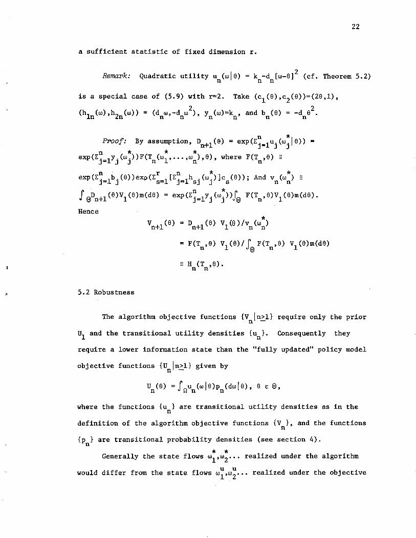
ZZ

a sufficient statistic of fixed dimension r.

Remark: Quadratic utility u (wle) = k -d [w_e]Z (cf. Theorem 5.Z) n n n

is a special case of (5.9) with r=Z. Take (cl(e),cZ(e»=(Ze,I),

(hln(w),hZn(w» = (dnw,-dnwZ), Yn(w)=kn , and bn(e) = -dne

Z.

n * Froof: By assumption, Dn+l(e) = eXP(Ej=IUj(Wjle» =

n * * * exp(E. ly.(w.»F(T (wl' .•• ,w ),e), where F(T ,e) :: J= J J n n n

n r n * * exp(E. Ib.(e»exp(E I[E. lh .(w.)]c (e»; And v (w ) -J= J s= J= sJ J s n n

J n * (' @Dn+l(e)VI(e)m(de) = exp(Ej=IYj(Wj»J@ F(Tn,e)VI(e)m(de).

Hence

5.Z Robustness

= F(T ,e) vl(e)/ J. F(T ,e) Vl(e)m(de) n @ n

:: H (T ,e). n n

The algorithm objective functions {Vnln~l} require only the prior

UI and the transitional utility densities {un}. Consequently they

require a lower information state than the "fully updated" policy model

objective functions {U In>l} given by n -

U (e) =J{"\u (wle)p (dwle), e e: @, nun n

where the functions {u } are transitional utility densities as in the n

definition of the algorithm objective functions {V}, and the functions n

{Pn} are transitional probability densities (see section 4).

* * Generally the state flows wl,wZ ... realized under the algorithm

would differ from the state flows w~,w~ ... realized under the objective

.,

23

functions {U}. However, if the state flows ware stochastically inde­n

pendent of present and past policy choices, i.e., for all wEn,eEe,n~l,

then presumably it would hold that

* * u u (wl ,w2 '···) = (wl ,w2 '···)·

In this case maximizing policy sets MV = {ev , ••• } n n

u u and M = {e , ••• } for n n

V and U can be simultaneously derived; and the relative robustness of n n

the algorithm can be measured by the differences

U (eu

) - U (ev), n~l, n n n n (5.10)

between "true" maximum expected utility for period n and "true" expected

utility corresponding to the policy choice eV selected to maximize the n

algorithm objective function V ,n>l. n -

In Theorem 5.7 below it will be shown that for a given sequence

* * wl

,w2

••• of "realized" state flows the differences in (5.10) are asymp-

totically negligible if the transitional utility assessments {u } n

eventually stabilize and the transitional probability assessments {Pn}

asymptotically approximate empirical frequencies. In Theorem 5.10 below

it will be shown that V asymptotically selects out the maximizing policy n

for U under essentially the same conditions. Theorems 5.7 and 5.10 n

therefore establish empirically meaningful conditions for the robustness

of the algorithm relative to the fully updated policy model objective

functions {U }, assuming state flows are stochastically independent of n

policy choices.

* * Notation: Let <i ,w2••• be a sequence of state flows realized over

periods 1,2... For any wEn and n~l, define

J

24

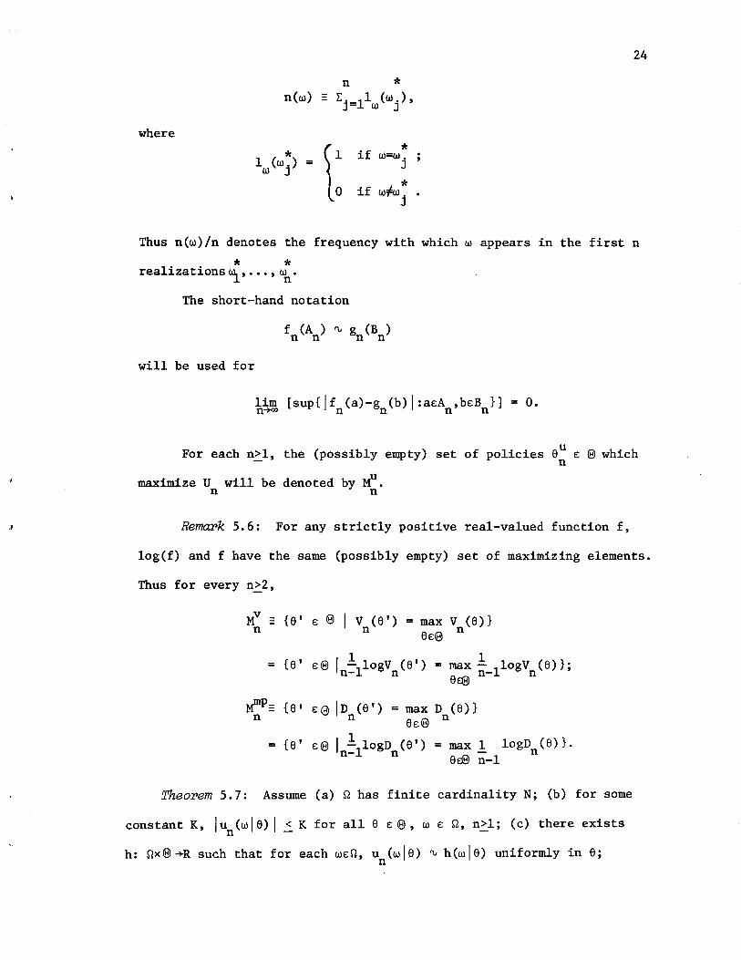
n * n(w) - Lj =llw(wj ),

where

* if w=w. J

* if W:fw. . J

Thus n(w)/n denotes the frequency with which w appears in the first n

* * realizations UJ.' ••• , wn •

The short-hand notation

f (A ) '" g (B ) n n n n

will be used for

lim [sup{lf (a)-g (b) I :aEA ,bEB }] = o. n+oo n n n n

For each n~l, the (possibly empty) set of policies aU E @ which n

u maximize U will be denoted by M . n n

Remark 5.6: For any strictly positive real-valued function f,

log(f) and f have the same (possibly empty) set of maximizing elements.

Thus for every n~2,

MV - {a' E @ I v (a') = max V (a)}

n n aE@ n

{a' I 1 1 = E@ -llogV (a') = max - 110gV (a)}; n- n n- n aee

~p= {a' E@ ID (a') = max D (a)} n n aE@ n

= {a' E@ I .! logD (a') = max 1 logD (a)}. n-1 n - n aee n-1

Theopem 5.7: Assume (a) Q has finite cardinality N; (b) for some

constant K, lun(wla) I.::. K for all a E@, w E Q, n~l; (c) there exists

h: Qx@-+R such that for each wEQ, u (wla) '" h(wla) uniformly in a; n

25

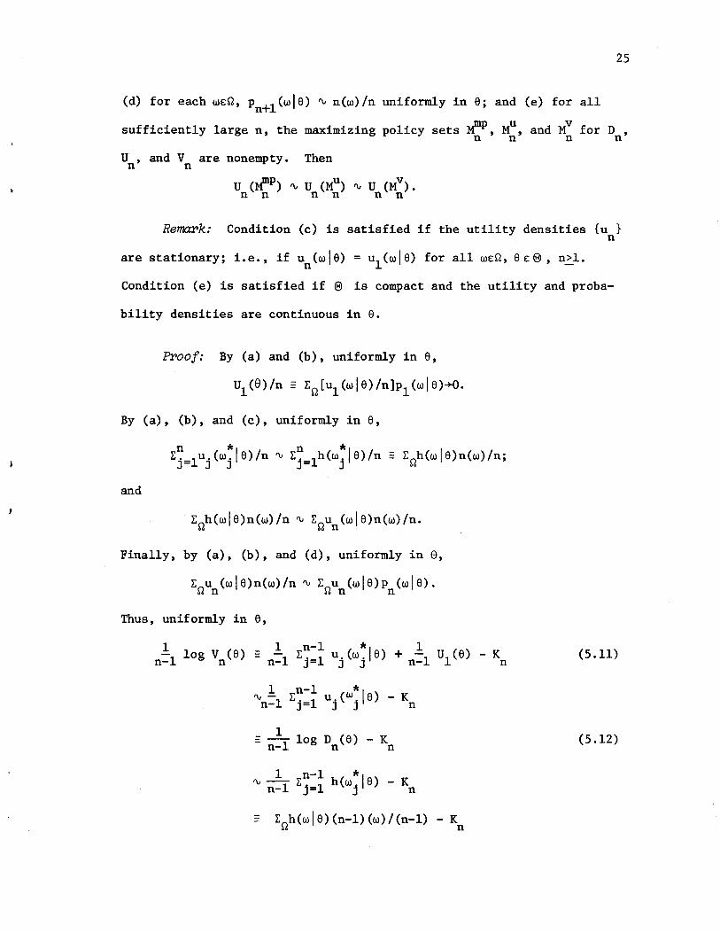
(d) for each wEQ, Pn+l(wle) ~ n(w)/n uniformly in e; and (e) for all

sufficiently large n, the maximizing policy sets ~P, MU, and MV for D , n n n n

U , and V are nonempty. Then n n

U (~p) ~ U (Mu) ~ U (Mv). n n n n n n

Remark: Condition (c) is satisfied if the utility densities {u } n

are stationary; Le., if un(wle) = ul(wle) for all wEQ, eE@, n~l.

Condition (e) is satisfied if @ is compact and the utility and proba-

bility densities are continuous in e.

Proof: By (a) and (b), uniformly in e,

By (a), (b), and (c), uniformly in e,

n *1 n *1 L. lU.(w. e)/n ~ L. lh(w. e)/n -J= J J J= J

and

Finally, by (a), (b), and (d), uniformly in 0,

L~U (wle)n(w)/n ~ L~U (wle)p (wi e). a6 n a6 n n

Thus, uniformly in e,

1 _ 1 n-l *1 1 -1 log V (e) = -1 L. 1 u.(w. e) + -1 ul(e) - K n- n n- J= J J n- n (5.11)

1 n-l *1 ~ -1 L. 1 u.(w. e) - K n- J= J J n

= ~ log D (8) - K n-l n n (5.12)

1 n-l * 1 ~ -1 L. 1 h (w. e) - K n- J= J n

'J

~ Enun(wla) (n-l) (w)/(n-l) - Kn

~ E~u (wla)p (wla) - K 06 n n n

:: U (a) - K • n n

By definition, the set of maximizing policies for (5.13)

Remark 5.6, the set of maximizing policies for (5.11) is

it is ~p. n

is MU•

n'

MV and n

26

(5.13)

and by

for (5.12)

Given £>0, it follows from the above that for sufficiently large n,

u (a) - ~ E~-l uJ.(wj*la) 1 < £/2 n n-l J=l

for all a £ @ • In particular, given any aU £ MU and amp £ ~p n n n n '

1 n-l *1 U + < n=l E. 1 u.(w. a) £/2 J= J J n

1 n-l *1 mp < -1 E. 1 uj(w. a ) + £/2 - n- J= J n

Since U (amp) < U (au) by definition of MU it follows that n n - n n n'

Thus

The proof for U (Mu) ~ U (M

v) is similar. n n n n

CoroUary 5.8: Assume (a) n and @ are finite; (b) U (w 1 a) ~ h(w 1 a) n

for all w £ n and a £ @ ; and (c) Pn+l(wla) ~ n(w)/n for all w £ nand

a £ @. Then

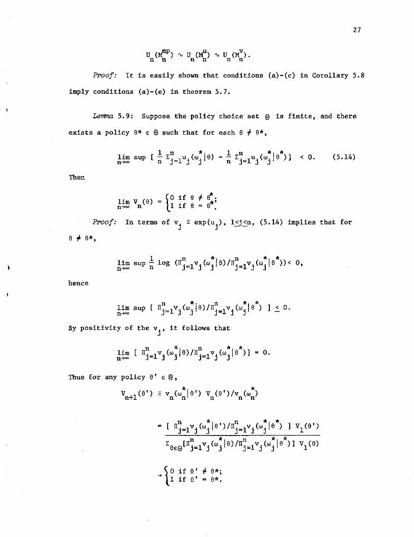
27

PFoof: It is easily shown that conditions (a)-(c) in Corollary 5.8

imply conditions (a)-(e) in theorem 5.7.

Lerrma 5.9: Suppose the policy choice set (8) is finite, and there

exists a policy 6* E (8) such that for each 6 ~ 6*,

Then

. 1 n *, 1 n *, * 11m sup [ - L._lu.(w. 6) - - L._luj(w. 6 )] n+oo n J- J J n J- J

lim V (6) = ~O ~f 6 ~ 6:; n+oo n t 1 1f 6 = 6 •

< O. (5.14)

PFoof: In terms of v. = exp(u.), l~j~n, (5.14) implies that for J J

6 ~ 6*,

hence

n *, n *, * lim sup [ IT._lv.(w. 6)/IT._l v.(w. 6 ) 0+00 J- J J J- J J

< O.

By positivity of the vj , it follows that

n *, n * * lim [ IT. IV. (w. 6) /IT. IV. (w., 6 )] = O. n+oo J= J J J= J J

Thus for any policy 6' E e, * * V +1(6') = v (w '6') V (6')/v (w ) n n n n n n

n *" n *, * , [ IT. lV'(w. 6 )/IT. lV'(w. 6 ) ] Vl (6 ) J= J J J= J J

n *, n *, * L6 ~[IT. lVj(w. 6)/IT. lV'(w. 6 )] Vl (6) EI!;!i J= J J= J J

s 0 if 6' :f 6*; -r II if 6' = 6*.

,

28

Theopem 5.10: Assume (a) Q and (8) are finite; (b) there exists

h:Qx(8)-+R such that un(wla) 'V h(wlE:t) for each we:Q and 8 e: (8); (c) Pn+1(wla)

'V n(w)/n for each we:Q and 8 e: (8); and (d) there exists a policy a* e: (8)

such that for each policy 8 ~ 8*,

Then

lim sup [U (8) - U (8*)] < O. n-+oo n n

lim V (8) = fo if 8 ~ a* ; n-+oo n (1 if 8 = 8* •

ppoof: Under conditions (a)-(c) it is easily shown (cf. theorem 5.7,

(5.11)-(5.13» that uniformly in a,

1 n *1 - L. 1u.(w. a) 'V U +1(8). n J= J J n

(5.15)

Together with condition (d), (5.15) implies

1 n *1 1 n *1 * lim sup [- L. 1u.(w. 8) - - L. 1u.(wj 8 )] < 0 n-+oo n J= J J n J= J

for 8 ~ 8*. The claim then follows from Lemma 5.9.

29

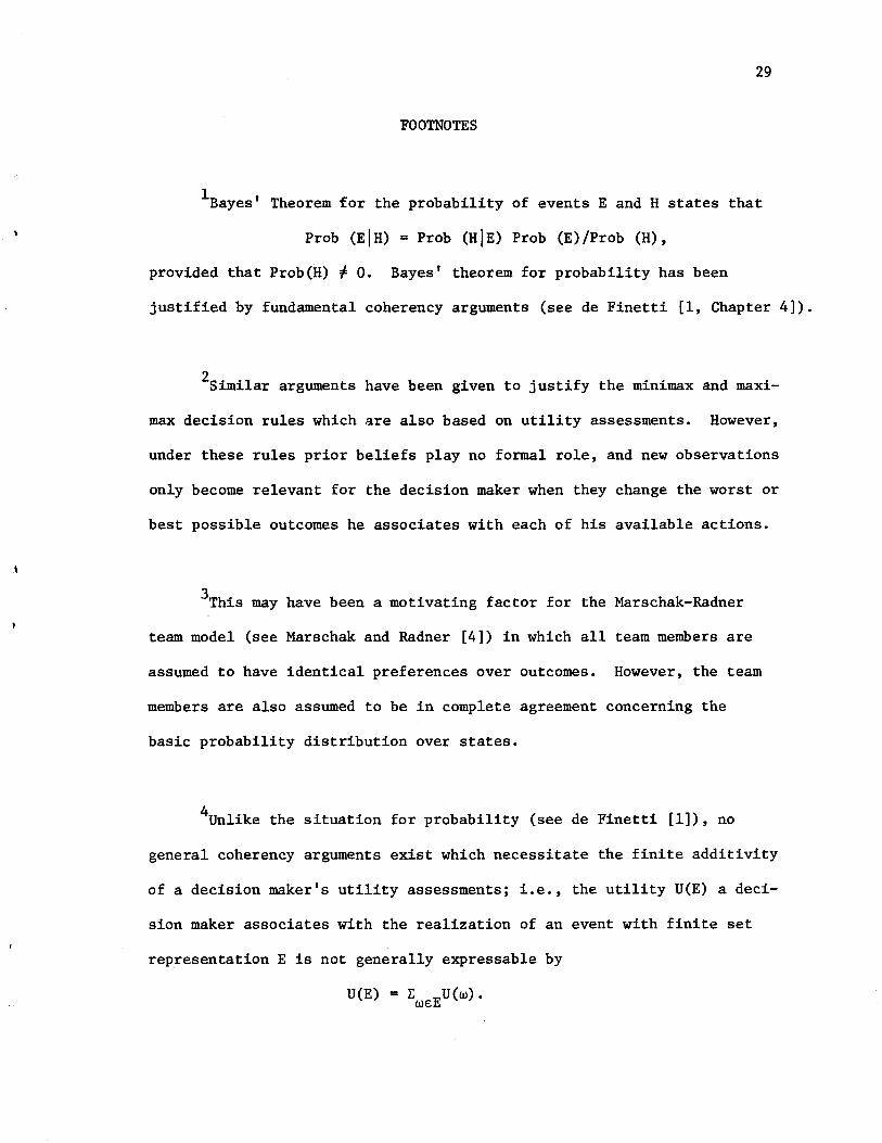
FOOTNOTES

1 Bayes' Theorem for the probability of events E and H states that

Prob (EIH) = Prob (HIE) Prob (E)/Prob (H),

provided that Prob(H) + O. Bayes' theorem for probability has been

justified by fundamental coherency arguments (see de Finetti [1, Chapter 4]).

2 Similar arguments have been given to justify the minimax and maxi-

max decision rules which are also based on utility assessments. However,

under these rules prior beliefs play no formal role, and new observations

only become relevant for the decision maker when they change the worst or

best possible outcomes he associates with each of his available actions.

3This may have been a motivating factor for the Marschak-Radner

team model (see Marschak and Radner [4]) in which all team members are

assumed to have identical preferences over outcomes. However, the team

members are also assumed to be in complete agreement concerning the

basic probability distribution over states.

4Unlike the situation for probability (see de Finetti [1]), no

general coherency arguments exist which necessitate the finite additivity

of a decision maker's utility assessments; i.e., the utility U(E) a deci-

sion maker associates with the realization of an event with finite set

representation E is not generally expressable by

U(E) = L EU(w). WE

30

On the other hand, it is the content of a number of expected utility

theories (e.g., see Jeffrey [3]) that a decision maker's utility assess-

ments are finitely additive with respect to some (probability) measure

P, appropriately conditioned; i.e.,

U(E) = L EU(w)P(w)/P(E). WE

5 The "policy model" presented in sections 2 and 3 is discussed in

greater detail in Tesfatsion [6] and [7]. As shown in Tesfatsion [6],

the expected utility model of Savage, the Marschak-Radner team model,

the Bayesian statistical decision model, and the standard optimal control

model can be viewed as special cases of the policy model. The policy

model is extended to a policy game in Tesfatsion [8] and shown to be a

generalization of the standard n-person game in normal form.

6A binary relation> on a set D is a weak order if for all a, b,

C E D

(1) a > b or b ~ a (i.e., ~ is connected);

(2) a > band b > c implies a > c (i.e., > is transitive).

7A collection F of subsets of a nonempty set X is said to be an

algebra in X if F has the following three properties:

(1) X E F;

c c (2) If A E F, then A E F, where A is the

complement of A relative to X;

(3) If A, B E F, then A U B £ F.

.\

:/

31

BIt will always be assumed that a decision maker's utility assess-

ments specified in an information state s known with certainty coincide

with the utility assessments he would make conditioned on that informa-

tion state; symbolically, u (w) = u(wls). Similarly for a decision s

maker's probability assessments. (The latter assumption is implicit in

nearly all Bayesian arguments.)

9 If the state flows ware not stochastically independent of policy

choices 6, then the reasoning implied by (4.2) can lead to undamped vacil-

lation between policies as the decision maker vainly attempts to achieve

certain state flow-policy matches. Costs incurred by switching policies

from period 1 to period 2 could be handled by the inclusion in the

* * of an additive cost term c(616 ), whe~e 61 is 1

the decision maker's first period policy choice. Such costs will not be

considered in this paper.

lOIn probability theory the use of uniform probability densities to

represent initial ignorance has often been criticized. For example, if

the decision maker is ignorant of the true value of 6 £ (0,00), then the

same must be said for the true value of 1/6. Yet the simultaneous speci-

fication of uniform probability densities over (0,00) for both 6 and 1/6

leads to contradiction. Moreover, uniform probability densities are often

"improper;" i. e., their associated distribution functions assign infinite

probability to the set of possible values.

In contrast, a uniform initial period objective function Ul un­

ambiguously represents the initial indifference of the decision maker

)

32

between available policy choices. Since utility assessments need not be

additive~ no contradictions arise. In particular, it is meaningless to

ask whether Ul

is "proper" or "improper."

REFERENCES

[1] de Finetti, B., Theory of Probability (Volume 1), New York: John Wiley

& Sons, Ltd., 1974.

[2] DeGroot, M. H., Optimal Statistical Decisions, New York: McGraw-Hill,

Inc., 1970.

[3] Jeffrey, R. C., The Logic of Decision, New York: McGraw Hill, Inc., 1965.

[4] Marschak, J. and Radner, R., Economic Theory of Teams, New Haven: Yale

University Press, 1972.

[5] Savage, L. J., The Foundations of Statistics, second revised edition,

New York: Dover Publications, Inc., 1972.

[6] Tesfatsion, L., "An Expected Utility Model with Endogenously Determined

Goals," Discussion Paper No. 75-58, Center for Economic Research,

University of Minnesota, September 1975.

[7] Tesfatsion, L., "Axiomatization for an Expected Utility Model With

Endogenously Determined Goals," Discussion Paper No. 75-59, Center

for Economic Research, University of Minnesota, September 1975.

[8] Tesfatsion, L., "Games,Goals, and Bounded Rationality," Discussion

Paper No. 76-63, Center for Economic Research, University of

Minnesota, January 1976.